Embed Size (px)
Citation preview
OPERATIONS RESEARCHVol. 55, No. 2, March–April 2007, pp. 252–271issn 0030-364X �eissn 1526-5463 �07 �5502 �0252
informs ®
doi 10.1287/opre.1060.0360©2007 INFORMS
Classification and Regression viaInteger Optimization
Dimitris BertsimasSloan School of Management and Operations Research Center, Massachusetts Institute of Technology,
E53-363, Cambridge, Massachusetts 02139, [email protected]
Romy ShiodaDepartment of Combinatorics and Optimization, Faculty of Mathematics, University of Waterloo,
Waterloo, Ontario, Canada N2L 3G1, [email protected]
Motivated by the significant advances in integer optimization in the past decade, we introduce mixed-integer optimizationmethods to the classical statistical problems of classification and regression and construct a software package called CRIO(classification and regression via integer optimization). CRIO separates data points into different polyhedral regions. Inclassification each region is assigned a class, while in regression each region has its own distinct regression coefficients.Computational experimentations with generated and real data sets show that CRIO is comparable to and often outperformsthe current leading methods in classification and regression. We hope that these results illustrate the potential for significantimpact of integer optimization methods on computational statistics and data mining.
Subject classifications : programming: integer, applications; statistics: nonparametric.Area of review : Financial Services.History : Received November 2002; revisions received April 2005, April 2006; accepted April 2006.
1. IntroductionIn the last 20 years, the availability of massive amountsof data in electronic form and the spectacular advances incomputational power have led to the development of thefield of data mining (or knowledge discovery) that is at thecenter of modern scientific computation. Two central prob-lems in this development (as well as in classical statistics)are data classification and regression. To the best of ourknowledge, popular methods for these problems include:(1) Decision trees for classification and regression
(Breiman et al. 1984). Decision trees recursively split thedata along a variable into hyper-rectangular regions. Afterthis forward propagation is complete, backward propaga-tion (or pruning) is performed to prevent over-fitting themodel to the data set. Its main shortcoming is its fundamen-tally greedy approach. Classification and regression trees(CART) (Breiman et al. 1984) is the leading work for thismodel. Bennett and Blue (1984) find a globally optimaldecision tree, but the structure of the tree needs to be pre-fixed. C5.0 (Quinlan 1993) is another popular method thatis similar in spirit to CART. CRUISE (Kim and Loh 2000)is a more recent version of CART that allows for multi-variate partitions (thus, heuristically partitioning the inputregions into polyhedral regions) and minimizes bias in thevariable selection step.(2) Multivariate adaptive regression splines (MARS)
(Friedman 1991) for regression. Like CART, MARS alsopartitions the data into regions but fits continuous splines orbasis functions to each region, thus maintaining continuityof the predicted values among neighboring regions.
(3) Support vector machines (SVM) (Vapnik 1999,Rifkin 2002, Mangasarian 1965) for classification. In itssimplest form, SVM separates points of different classesby a single hyperplane. More sophisticated SVM methodsfind a separating hyperplane in a higher dimensional space,leading to a nonlinear partitioning. In all cases, the opti-mal separating hyperplane is modeled as a convex quadraticprogramming problem.Decision trees and MARS are heuristics in nature and
are closer to the tradition of statistical inference meth-ods. SVM belongs to the category of separating hyperplanemethods, utilize formal continuous optimization techniques(quadratic optimization), and are closer to the tradition ofmachine learning and mathematical programming. It is fairto say that all these methods (to various degrees) are at theforefront of data mining and have had significant impact inpractical applications. Commercial software is available forall these methods, facilitating their wide applicability.While continuous optimization methods have been
widely used in statistics and have had a significant impactin the last 30 years (a classical reference is Arthanari andDodge 1993), integer optimization has had very limitedimpact in statistical computation. While the statistics com-munity has long recognized that many statistical problems,including classification and regression, can be formulatedas integer optimization problems (Arthanari and Dodge1993 contains several integer optimization formulations),the belief was formed in the early 1970s that these meth-ods are not tractable in practical computational settings.Due to the success of the above methods and the belief
252
Bertsimas and Shioda: Classification and Regression via Integer OptimizationOperations Research 55(2), pp. 252–271, © 2007 INFORMS 253
of integer optimization’s impracticality, the applicability ofinteger optimization methods to the problems of classifica-tion and regression has not been seriously investigated.Our objective in this paper is to do exactly this—to
develop a methodology for classification and regressionthat utilizes state-of-the-art integer optimization methods toexploit the discrete character of these problems. We weremotivated by the significant advances in integer optimiza-tion in the past decade that make it possible to solve large-scale problems within practical times. We have created asoftware package based on integer optimization that wecall classification and regression via integer optimization(CRIO), which we compare to the state-of-the-art meth-ods outlined earlier. While CRIO’s distinguishing featureis mixed-integer optimization, we have incorporated certainelements of earlier methods that have been successful inour attempt to make CRIO applicable in diverse real-worldsettings.We view our contribution as twofold:(1) To bring to the attention of the statistics and data
mining community that integer optimization can have a sig-nificant impact on statistical computation, and thus moti-vate researchers to revisit old statistical problems usinginteger optimization.(2) To show that CRIO is a promising method for classi-
fication and regression that matches and often outperformsother state-of-the-art methods outlined earlier.The structure of this paper is as follows. In §2, we
give an intuitive presentation of the geometric ideas of ourapproach for both classification and regression to facili-tate understanding, and provide motivation to the globallyoptimal nature of CRIO. In §§3 and 4, we develop CRIOfor classification and for regression, respectively. In §5, wecompare CRIO with logistic regression, least-square regres-sion, neural networks, decision trees, SVMs, and MARSon generate and real data sets. We present our conclusionsin the final section.
2. An Intuitive Overview of CRIOIn this section, we present the geometric ideas of ourapproach intuitively (first with respect to classification andthen with respect to regression) to facilitate understandingof the mathematical presentation in §§3 and 4.
2.1. The Geometry of the Classification Approach
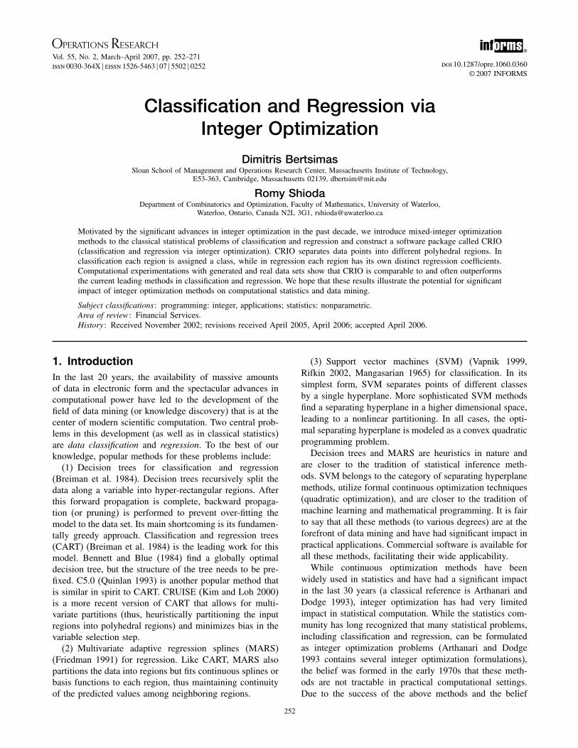
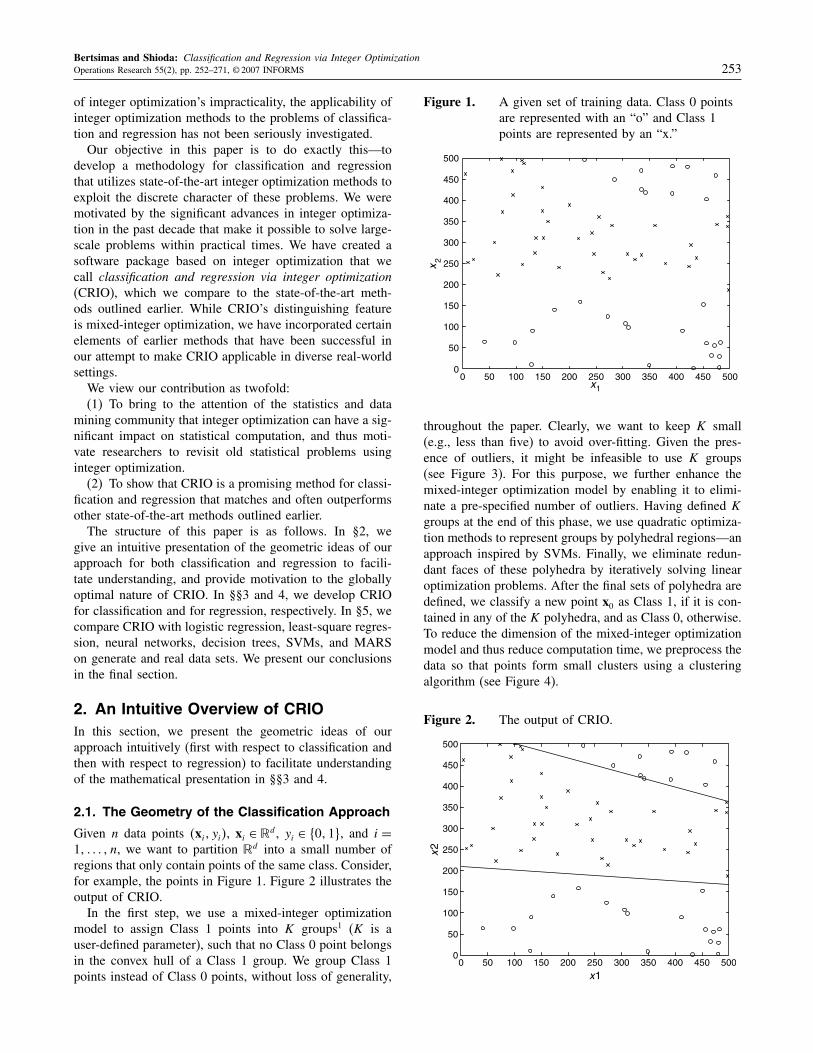
Given n data points �xi� yi�, xi ∈ �d, yi ∈ �0�1, and i =1� � n, we want to partition �d into a small number ofregions that only contain points of the same class. Consider,for example, the points in Figure 1. Figure 2 illustrates theoutput of CRIO.In the first step, we use a mixed-integer optimization
model to assign Class 1 points into K groups1 (K is auser-defined parameter), such that no Class 0 point belongsin the convex hull of a Class 1 group. We group Class 1points instead of Class 0 points, without loss of generality,
Figure 1. A given set of training data. Class 0 pointsare represented with an “o” and Class 1points are represented by an “x.”
0 50 100 150 200 250 300 350 400 450 5000
50
100
150
200
250
300
350
400
450
500
x1
x2
throughout the paper. Clearly, we want to keep K small(e.g., less than five) to avoid over-fitting. Given the pres-ence of outliers, it might be infeasible to use K groups(see Figure 3). For this purpose, we further enhance themixed-integer optimization model by enabling it to elimi-nate a pre-specified number of outliers. Having defined Kgroups at the end of this phase, we use quadratic optimiza-tion methods to represent groups by polyhedral regions—anapproach inspired by SVMs. Finally, we eliminate redun-dant faces of these polyhedra by iteratively solving linearoptimization problems. After the final sets of polyhedra aredefined, we classify a new point x0 as Class 1, if it is con-tained in any of the K polyhedra, and as Class 0, otherwise.To reduce the dimension of the mixed-integer optimizationmodel and thus reduce computation time, we preprocess thedata so that points form small clusters using a clusteringalgorithm (see Figure 4).
Figure 2. The output of CRIO.
0 50 100 150 200 250 300 350 400 450 5000
50
100
150
200
250
300
350
400
450
500
x1
x2
Bertsimas and Shioda: Classification and Regression via Integer Optimization254 Operations Research 55(2), pp. 252–271, © 2007 INFORMS
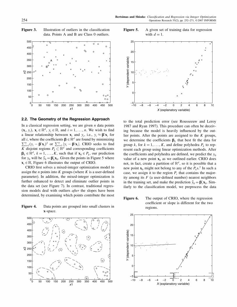
Figure 3. Illustration of outliers in the classificationdata. Points A and B are Class 0 outliers.
0 50 100 150 200 250 300 350 400 450 5000
50
100
150
200
250
300
350
400
450
500
x1
x2
A
B
2.2. The Geometry of the Regression Approach
In a classical regression setting, we are given n data points�xi� yi�, xi ∈ �d, yi ∈ �, and i = 1� � n. We wish to finda linear relationship between xi and yi, i.e., yi ≈ �′xi forall i, where the coefficients � ∈�d are found by minimizing∑n
i=1�yi − �′xi�2 or
∑ni=1 �yi − �′xi�. CRIO seeks to find
K disjoint regions Pk ⊂ �d and corresponding coefficients�k ∈ �d, k = 1� �K, such that if x0 ∈ Pk, our predictionfor y0 will be �y0 = �′
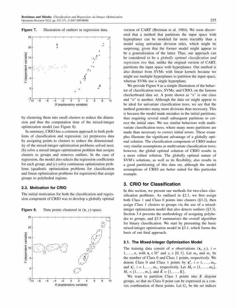
kx0. Given the points in Figure 5 wherexi ∈�, Figure 6 illustrates the output of CRIO.CRIO first solves a mixed-integer optimization model to
assign the n points into K groups (where K is a user-definedparameter). In addition, the mixed-integer optimization isfurther enhanced to detect and eliminate outlier points inthe data set (see Figure 7). In contrast, traditional regres-sion models deal with outliers after the slopes have beendetermined, by examining which points contribute the most
Figure 4. Data points are grouped into small clusters inx-space.
0 50 100 150 200 250 300 350 400 450 5000
50
100
150
200
250
300
350
400
450
500
x1
x2
Figure 5. A given set of training data for regressionwith d = 1.
–10 –8 –6 –4 –2 0 2 4 6 8 10–5
0
5
10
15
20
25
X (explanatory variable)
Y (
depe
nden
t var
iabl
e)
to the total prediction error (see Rousseeuw and Leroy1987 and Ryan 1997). This procedure can often be deceiv-ing because the model is heavily influenced by the out-lier points. After the points are assigned to the K groups,we determine the coefficients �k that best fit the data forgroup k, for k = 1� �K, and define polyhedra Pk to rep-resent each group using linear optimization methods. Afterthe coefficients and polyhedra are defined, we predict the y0value of a new point x0 as we outlined earlier. CRIO doesnot, in fact, create a partition of �d, so it is possible that anew point x0 might not belong to any of the Pks.
2 In such acase, we assign it to the region Pr that contains the major-ity among its F (a user-defined number) nearest neighborsin the training set, and make the prediction �y0 = �′
rx0. Sim-ilarly to the classification model, we preprocess the data
Figure 6. The output of CRIO, where the regressioncoefficient or slope is different for the tworegions.
–10 –8 –6 –4 –2 0 2 4 6 8 10–5
0
5
10
15
20
25
X (explanatory variable)
Y (
depe
nden
t var
iabl
e)
Bertsimas and Shioda: Classification and Regression via Integer OptimizationOperations Research 55(2), pp. 252–271, © 2007 INFORMS 255
Figure 7. Illustration of outliers in regression data.
–10 –8 –6 –4 –2 0 2 4 6 8 10–5
0
5
10
15
20
25
X (explanatory variable)
Y (
depe
nden
t var
iabl
e)
A
B
by clustering them into small clusters to reduce the dimen-sion and thus the computation time of the mixed-integeroptimization model (see Figure 8).In summary, CRIO has a common approach to both prob-
lems of classification and regression: (a) preprocess databy assigning points to clusters to reduce the dimensional-ity of the mixed-integer optimization problems solved next;(b) solve a mixed integer-optimization problem that assignsclusters to groups and removes outliers. In the case ofregression, the model also selects the regression coefficientsfor each group; and (c) solve continuous optimization prob-lems (quadratic optimization problems for classificationand linear optimization problems for regression) that assigngroups to polyhedral regions.
2.3. Motivation for CRIO
The initial motivation for both the classification and regres-sion component of CRIO was to develop a globally optimal
Figure 8. Data points clustered in �x� y�-space.
–10 –8 –6 –4 –2 0 2 4 6 8 10–5
0
5
10
15
20
25
X (explanatory variable)
Y (
depe
nden
t var
iabl
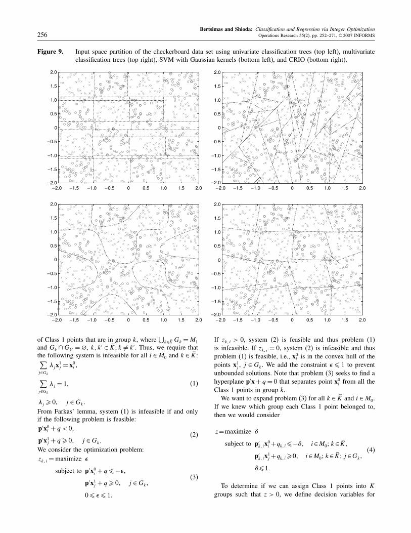
e)version of CART (Breiman et al. 1984). We soon discov-ered that a method that partitions the input space withhyperplanes can be modeled far more tractably than amodel using univariate division rules, which might besurprising, given that the former model might appear tobe a generalization of the latter. Thus, our approach canbe considered to be a globally optimal classification andregression tree that, unlike the original version of CART,partitions the input space with hyperplanes. Our method isalso distinct from SVMs with linear kernels because wemight use multiple hyperplanes to partition the input space,whereas SVMs use a single hyperplane.We provide Figure 9 as a simple illustration of the behav-
ior of classification trees, SVMs, and CRIO, on the famouscheckerboard data set. A point shown as “x” is one classand “o” is another. Although the data set might appear tobe ideal for univariate classification trees, we see that themethod generates many more divisions than necessary. Thisis because the model made mistakes in the initial partitions,thus requiring several small subsequent partitions to cor-rect the initial ones. We see similar behaviors with multi-variate classification trees, where many more partitions aremade than necessary to correct initial errors. These exam-ples illustrate the significant advantage of a globally opti-mal solution. The classification component of CRIO makesvery similar assumptions as multivariate classification trees;however, the global optimal solution of CRIO results ina more robust solution. The globally optimal nature ofSVM’s solutions, as well as its flexibility, also results ina good partitioning of this data set, although the modelassumptions of CRIO are better suited for this particularexample.
3. CRIO for ClassificationIn this section, we present our methods for two-class clas-sification problems. As outlined in §2.1, we first assignboth Class 1 and Class 0 points into clusters (§3.2), thenassign Class 1 clusters to groups via the use of a mixed-integer optimization model that also detects outliers (§3.3).Section 3.4 presents the methodology of assigning polyhe-dra to groups, and §3.5 summarizes the overall algorithmfor binary classification. We start by presenting the basicmixed-integer optimization model in §3.1, which forms thebasis of our final approach.
3.1. The Mixed-Integer Optimization Model
The training data consist of n observations �xi� yi�, i =1� � n, with xi ∈ �d and yi ∈ �0�1. Let m0 and m1 bethe number of Class 0 and Class 1 points, respectively. Wedenote Class 0 and Class 1 points by x0i , i = 1� �m0,and x1i , i = 1� �m1, respectively. Let M0 = �1� �m0,M1 = �1� �m1, and K = �1� �K.We want to partition Class 1 points into K disjoint
groups, so that no Class 0 point can be expressed as a con-vex combination of these points. Let Gk be the set indices
Bertsimas and Shioda: Classification and Regression via Integer Optimization256 Operations Research 55(2), pp. 252–271, © 2007 INFORMS
Figure 9. Input space partition of the checkerboard data set using univariate classification trees (top left), multivariateclassification trees (top right), SVM with Gaussian kernels (bottom left), and CRIO (bottom right).
–0.5 0 0.5 1.0 1.5 2.0–2.0
–2.0
–1.5
–1.5
–1.0
–1.0
–0.5
0
0.5
1.0
1.5
2.0
–0.5 0 0.5 1.0 1.5 2.0–2.0
–2.0
–1.5
–1.5
–1.0
–1.0
–0.5
0
0.5
1.0
1.5
2.0
–0.5 0 0.5 1.0 1.5 2.0–2.0
–2.0
–1.5
–1.5
–1.0
–1.0
–0.5
0
0.5
1.0
1.5
2.0
–0.5 0 0.5 1.0 1.5 2.0–2.0
–2.0
–1.5
–1.5
–1.0
–1.0
–0.5
0
0.5
1.0
1.5
2.0
of Class 1 points that are in group k, where⋃
k∈ K Gk =M1
and Gk ∩Gk′ = �, k�k′ ∈ K�k �= k′. Thus, we require thatthe following system is infeasible for all i ∈M0 and k ∈ K:∑j∈Gk
�jx1j = x0i �
∑j∈Gk
�j = 1�
�j � 0� j ∈Gk
(1)
From Farkas’ lemma, system (1) is infeasible if and onlyif the following problem is feasible:p′x0i + q < 0�
p′x1j + q � 0� j ∈Gk(2)
We consider the optimization problem:zk� i =maximize �
subject to p′x0i + q �−��
p′x1j + q � 0� j ∈Gk�
0� � � 1
(3)
If zk� i > 0, system (2) is feasible and thus problem (1)is infeasible. If zk� i = 0, system (2) is infeasible and thusproblem (1) is feasible, i.e., x0i is in the convex hull of thepoints x1j , j ∈ Gk. We add the constraint � � 1 to preventunbounded solutions. Note that problem (3) seeks to find ahyperplane p′x+ q = 0 that separates point x0i from all theClass 1 points in group k.We want to expand problem (3) for all k ∈ K and i ∈M0.
If we knew which group each Class 1 point belonged to,then we would consider
z=maximize �
subject to p′k� ix
0i +qk�i�−�� i∈M0� k∈ K�
p′k� ix
1j +qk�i�0� i∈M0� k∈ K� j ∈Gk�
��1
(4)
To determine if we can assign Class 1 points into K
groups such that z > 0, we define decision variables for
Bertsimas and Shioda: Classification and Regression via Integer OptimizationOperations Research 55(2), pp. 252–271, © 2007 INFORMS 257
k ∈ K and j ∈M1:
ak� j =1 if x1j is assigned to group k (i.e., j ∈Gk��
0 otherwise.(5)
We include the constraints p′k� ix
1j + qk� i � 0 in problem (4)
if and only if ak� j = 1, i.e.,
p′k� ix
1j + qk� i �M�ak� j − 1��
where M is a large positive constant. Note, however, thatwe can re-scale the variables pk� i and qk� i by a positivenumber, and thus we can take M = 1, i.e.,
p′k� ix
1j + qk� i � ak� j − 1
Thus, we can check whether we can partition Class 1points into K disjoint groups such that no Class 0 pointsare included in their convex hull, by solving the followingmixed-integer optimization problem:
z∗ =maximize �
subject to p′k� ix
0i + qk� i �−�� i ∈M0� k ∈ K�
p′k� ix
1j + qk� i � ak� j − 1�
i ∈M0� k ∈ K� j ∈M1�∑Kk=1 ak� j = 1� j ∈M1�
�� 1�
ak� j ∈ �0�1
(6)
If z∗ > 0, the partition into K groups is feasible; while ifz∗ = 0, it is not, requiring us to increase the value of K.
3.2. The Clustering Algorithm
Problem (6) has Km0�d+1�+1 continuous variables, Km1
binary variables, and Km0 +Km0m1 +m1 rows. For largevalues of m0 and m1, problem (6) becomes expensive tosolve. Alternatively, we can drastically decrease the dimen-sion of problem (6) by solving a hyperplane for clusters ofpoints at a time instead of point by point.We develop a hierarchical clustering-based algorithm that
preprocesses the data to create clusters of Class 0 andClass 1 points. Collections of Class 0 (Class 1) pointsare considered a cluster if there are no Class 1 (Class 0)points in their convex hull. If we preprocess the data tofind K0 Class 0 clusters and K1 Class 1 clusters, we canmodify problem (6) (see formulation (9) below) to haveKK0�d+1�+1 continuous variables, KK1 binary variables,and Km0+KK0m1+K1 rows.The clustering algorithm applies the hierarchical cluster-
ing methodology (see Johnson and Wichern 1998) wherepoints or clusters with the shortest distances are mergedinto a cluster until the desired number of clusters is
achieved. For our purposes, we need to check whether amerger of Class 0 (Class 1) clusters will not contain anyClass 1 (Class 0) points in the resulting convex hull. Wesolve the following linear optimization problem to checkwhether Class 1 clusters r and s can be merged:
�∗ =maximize �
subject to p′ix0i + qi �−�� i ∈M0�
p′ix1j + qi � �� j ∈Cr ∪Cs�
(7)
where Cr and Cs are the set of indices of Class 1 points inclusters r and s, respectively.If �∗ > 0, then clusters r and s can merge; while if �∗ =
0, they cannot because there is at least one Class 0 pointin the convex hull of the combined cluster. The overallpreprocessing algorithm that identifies clusters of Class 1points is as follows:
1. Initialize: K �=m1, k �= 0.2. while k < K do3. Find the clusters with minimum pairwise
distance—call these r and s.4. Solve problem (7) on clusters r and s.5. if �∗ = 0 then6. k �= k+ 17. else8. Merge clusters r and s.9. K �=K − 1, k �= 0.10. end if11. k �= k+ 1.12. end while
In the start of the algorithm, each point is considered acluster, thus K =m1. On line 3, the minimum pairwise dis-tances are calculated by comparing the statistical distances3
between the centers of all the clusters. We define the centerof a cluster as the arithmetic mean of all the points thatbelong to that cluster. In the merging step on line 4, thesecenters are updated. Finding clusters for Class 0 followssimilarly.After we have K0 and K1 clusters of Class 0 and Class 1
points, respectively, we run a modified version of problem(6) to assign the K1 Class 1 clusters to K groups, whereK < K1 �m1. Let K0 = �1� �K0 and K1 = �1� �K1.Let C0
t , t ∈ K0, be the set of indices of Class 0 points incluster t and C1
r , r ∈ K1, be the set of indices of Class 1points in Cluster r . We define the following binary vari-ables for r ∈ K1 and k ∈ K:
ak� r ={1 if cluster r is assigned to group k�
0 otherwise.(8)
Analogously to problem (6), we formulate the followingmixed-integer optimization problem for clusters:
maximize �
subject to p′k� tx
0i + qk� t �−�� i ∈C0
t � t ∈ K0� k ∈ K�
Bertsimas and Shioda: Classification and Regression via Integer Optimization258 Operations Research 55(2), pp. 252–271, © 2007 INFORMS
p′k� tx
1j + qk� t � ak� r − 1�
t ∈ K0� r ∈ K1� k ∈ K� j ∈C1r �
K∑k=1
ak� r = 1� r ∈ K1�
ak� r ∈ �0�1(9)
If ak� r = 1 in an optimal solution, then all Class 1 points incluster r are assigned to group k, i.e., Gk =
⋃�r �ak� r=1 C
1r .
3.3. Elimination of Outliers
In the presence of outliers, it is possible that we may needa large number of groups—possibly leading to over-fitting.A point can be considered an outlier if it lies significantlyfar from any other point of its class (see Figure 3 for anillustration). In this section, we outline two methods thatremove outliers: (a) based on the clustering algorithm of theprevious section, and (b) via an extension of problem (9).
Outlier Removal via Clustering. The clustering me-thod of §3.2 applied on Class 0 points would keep outlierpoints in its own cluster without ever merging them withany other Class 0 cluster. Thus, after K0 clusters are found,we can check the cardinality of each of the clusters andeliminate those with very small cardinality—perhaps lessthan 1% of m0. Such a procedure can similarly be done onClass 1 points.
Outlier Removal via Optimization. Figure 3 illus-trates how outlier points can prevent CRIO from groupingClass 1 points with small K, i.e., problem (9) can returnonly a trivial solution where � = 0, pk� i = 0, qk� i = 0, andthe ak� js are assigned arbitrarily. We want to modify prob-lem (9) to eliminate or ignore outlier points that prevent usfrom grouping Class 1 points into K groups.One possible approach is to assign a binary decision vari-
able to each point, so that it is removed if it is equal toone and not removed otherwise. Such a modification canbe theoretically incorporated into formulation (9), but thelarge increase in binary variables can make the problemdifficult to solve.We propose a different approach that modifies problem
(9) to always return a partition of Class 1 points so that thetotal margin of the violation is minimized. Problem (10)is such a model, where �0i and �1j are violation marginscorresponding to Class 0 and Class 1 points, respectively.The model is as follows:
minimizem0∑i=1
�0i +m1∑j=1
�1j
subject to p′k�tx
0i +qk�t �−1+�0i � i∈C0
t � t∈ K0� k∈ K�
p′k� tx
1j + qk� t �−M + �M + 1�ak� r − �1j �
t ∈ K0� k ∈ K� r ∈ K1� j ∈C1r �
K∑k=1
ak� r = 1� r ∈ K1�
ak� r ∈ �0�1� �0i � 0� �1j � 0�(10)
where M is a large positive constant.As in problem (9), the first constraint of problem (10)
requires p′k� tx
0i + qk� t to be strictly negative for all Class
0 points. However, if a point x0i cannot satisfy the con-straint, problem (10) allows the constraint to be violated,i.e., p′
k� tx0i + qk� t can be positive if �0i > 1. Similarly, prob-
lems (9) and (10) require p′k� tx
1j + qk� t to be nonnegative
when ak� r = 1 and arbitrary when ak� r = 0. However, (10)allows p′
k� tx1j + qk� t to be negative even when ak� r = 1
because the second constraint becomes p′k� tx
1j + qk� t � 1−
�1j when ak� r = 1, and the left-hand side can take on neg-ative values if �1j > 1. Thus, by allowing �0i and �1j to begreater than one when necessary, problem (10) will alwaysreturn K Class 1 groups by ignoring those points that ini-tially prevented the groupings. These points with �0i > 1and �1j > 1 can be considered outliers and be eliminated.
3.4. Assigning Groups to Polyhedral Regions
The solution of problem (10) results in K disjoint groups ofClass 1 points, such that no Class 0 point is in the convexhull of any of these groups. Our objective in this sectionis to represent each group k geometrically with a polyhe-dron Pk. An initially apparent choice for Pk is to use thesolution of problem (10), i.e.,
Pk = �x ∈�d � p′k� tx�−qk� t� k ∈ K� t ∈ K0
Motivated by the success of SVMs (see Vapnik 1999),we present an approach of using hyperplanes that separatethe points of each class such that the minimum Euclideandistance from any point to the hyperplane is maximized.This prevents over-fitting the model to the training data setbecause it leaves as much distance between the boundaryand points of each class as possible.Our goal is to find a hyperplane
�′k� tx= !k� t
for every group k, k ∈ K, of Class 1 points and for everycluster t, t ∈ K0, of Class 0 points such that all points incluster t are separated from every point in group k so thatthe minimum distance between every point and the hyper-plane is maximized. The distance, d�x��k� t�!k� t�, betweena point x and the hyperplane �′
k� tx= !k� t , is
d�x��k� t�!k� t�=�"�
��k� t�� where " =�′
k� tx−!k� t
Thus, we can maximize d�x��k� t�!k� t� by fixing �"� andminimize ��k� t�2 = �′
k� t�k� t , thus solving the quadraticoptimization problem:
minimize �′k� t�k� t
subject to �′k� tx
0i � !k� t + 1� i ∈C0
t �
�′k� tx
1j � !k� t − 1� j ∈Gk
(11)
Bertsimas and Shioda: Classification and Regression via Integer OptimizationOperations Research 55(2), pp. 252–271, © 2007 INFORMS 259
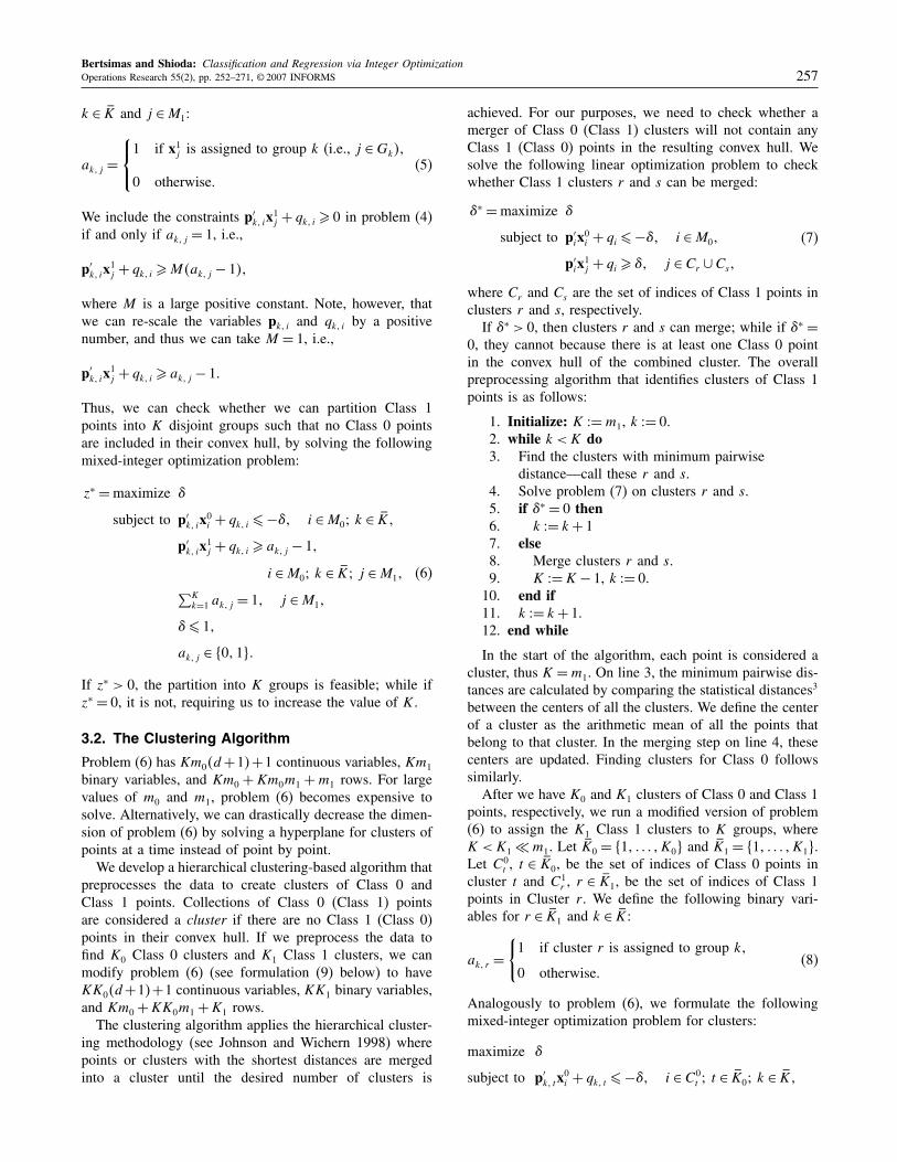
Figure 10. Before eliminating redundant constraints.
0 50 100 150 200 250 300 350 400 450 5000
50
100
150
200
250
300
350
400
450
500
x1
x2
We solve problem (11) for each t ∈ K0 and k ∈ K, and findKK0 hyperplanes. Thus, for each group k, the correspond-ing polyhedral region is
Pk = �x ∈�d ��′k� tx� !k� t� t ∈ K0 (12)
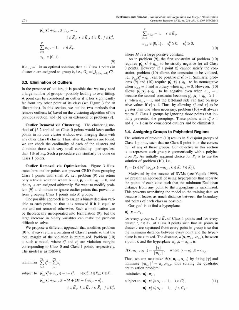
The last step in our process is the elimination of redundanthyperplanes in the representation of polyhedron Pk given inEquation (12). Figures 10 and 11 illustrate this procedure.We can check whether the constraint
�′k� t0
x� !k� t0(13)
is redundant for the representation of Pk by solving the fol-lowing linear optimization problem (note that the decisionvariables are x):
wk� t0=maximize �′
k� t0x
subject to �′k� tx� !k� t� t ∈ K0\�t0�
�′k� t0
x� !k� t0+ 1
(14)
Figure 11. After eliminating redundant constraints.
0 50 100 150 200 250 300 350 400 450 5000
50
100
150
200
250
300
350
400
450
500
x1
x2
We have included only the last constraint to prevent prob-lem (14) from becoming unbounded. If wk� t0
� !k� t0, then
constraint (13) is implied by the other constraints defin-ing Pk, and thus it is redundant. However, if wk� t0
> !k� t0,
then constraint (13) is necessary for describing the polyhe-dron Pk. To summarize, the following algorithm eliminatesall redundant constraints.
1. for k = 1 to K do2. for t0 = 1 to K0 do3. Solve problem (14).4. if wk� t0
� !k� t0then
5. Eliminate constraint �′k� t0
x� !k� t0.
6. end if7. end for8. end for
3.5. The Overall Algorithm for Classification
The overall algorithm for classification is as follows:
1. Preprocessing. Use the clustering algorithm outlinedin §3.2 to find clusters. Eliminate clusters with cardinalityless than 1% of m0 (m1) for Class 0 (Class 1) clusters.2. Assign clusters to groups. Solve the mixed-integer
optimization problem (10) to assign clusters of Class 1points to groups, while eliminating potential outliers.3. Assign groups to polyhedral regions. Solve the
quadratic optimization problem (11) to find hyperplanesthat define the polyhedron of each Class 1 group.4. Eliminate redundant constraints. Remove redun-
dant constraints from the polyhedra following the algorithmoutlined at the end of §3.4.
After CRIO determines the nonredundant representationsof the polyhedra, the model is used to predict the class ofnew data points. If the point lies in any of the K polyhedra,we label the point as a Class 1 point. If the point is notcontained in any of the polyhedra, then we label the pointas a Class 0 point.
4. CRIO for RegressionIn this section, we present in detail our approach for regres-sion. For presentation purposes, we start in §4.1 with aninitial mixed-integer optimization model to assign points togroups, which, while not practical because of dimensional-ity problems, forms the basis of our approach. As outlinedin §2.2, we first assign points to clusters (§4.2), then assignclusters to groups of points (§4.3), which we then repre-sent by polyhedral regions Pk (§4.4). In §4.5, we proposea method of automatically finding nonlinear transforma-tions of the explanatory variables to improve the predictivepower of the method. Finally, we present the overall algo-rithm in §4.6.
4.1. Assigning Points to Groups: An Initial Model
The training data consist of n observations �xi� yi�, i =1� � n, with xi ∈ �d and yi ∈ �. We let N = �1� � n,
Bertsimas and Shioda: Classification and Regression via Integer Optimization260 Operations Research 55(2), pp. 252–271, © 2007 INFORMS
K = �1� �K, and M be a large positive constant. Wedefine binary variables for k ∈ K and i ∈N :
ak� i =1 if xi is assigned to group k�
0 otherwise.
The mixed-integer optimization model is as follows:
minimizen∑
i=1�i
subject to �i � �yi −�′kxi�−M�1− ak� i�� k ∈ K� i ∈N�
�i�−�yi−�′kxi�−M�1−ak�i�� k∈ K� i∈N�
K∑k=1
ak� i = 1� i ∈N�
ak� i ∈ �0�1� �i � 0(15)
From the first and second constraints, �i is the absoluteerror associated with point xi. If ak� i = 1, then �i � �yi −�′
kxi�, �i �−�yi −�′kxi�, and the minimization of �i sets �i
equal to �yi − �′kxi�. If ak� i = 0, the right-hand side of the
first two constraints becomes negative, making them irrele-vant because �i is nonnegative. Finally, the third constraintlimits the assignment of each point to just one group.We have found that even for relatively small n (n≈ 200),
problem (15) is difficult to solve in reasonable time. Forthis reason, we initially run a clustering algorithm, similarto that of §3.2, to cluster nearby xi points together. After Lsuch clusters are found, for L� n, we can solve a mixed-integer optimization model, similar to problem (15), butwith significantly fewer binary decision variables.
4.2. The Clustering Algorithm
We apply a nearest-neighbor clustering algorithm in thecombined �x� y� space, as opposed to just the x space, tofind L clusters. Specifically, the clustering algorithm ini-tially starts with n clusters, then continues to merge theclusters with points close to each other until we are leftwith L clusters. More formally, the clustering algorithm isas follows:
1. Initialize: k = n. Ci = �i, i = 1� � n.2. while l < L do3. Find the points �xi� yi� and �xj � yj�, i < j , with
minimum pairwise statistical distance. Let l�i�and l�j� be the indices of the clusters that �xi� yi�and �xj � yj� currently belong to, respectively.
4. Add cluster l�j�’s points to cluster l�i�,i.e., Cl�i� �=Cl�i� ∪Cl�j�.
5. Let the pairwise statistical distance betweenall the points in Cl�i� be �.
6. l = l− 1.7. end while
In the clustering algorithm for classification problems(§3.2), we merged clusters that had centers of close proxim-ity. However, in the present clustering algorithm, we mergeclusters that contain points of close proximity. Computa-tional experimentations showed that this latter method ofclustering suited the regression problem better.
4.3. Assigning Points to Groups: A PracticalApproach
Although we can continue the clustering algorithm of theprevious section until we find K clusters, define them asour final groups, and find the best �k coefficient for eachgroup by solving separate linear regression problems, suchan approach does not combine points to minimize the totalabsolute error. For this reason, we use the clustering algo-rithm until we have L, L > K, clusters and then solve amixed-integer optimization model that assigns the L clus-ters into K groups to minimize the total absolute error.Another key concern in regression models is the pres-ence of outliers. The mixed-integer optimization model wepresent next is able to remove potential outliers by elimi-nating points in clusters that tend to weaken the fit of thepredictor coefficients.Let Cl, l ∈ L̄ = �1� �L, be cluster l, and denote l�i�
as xi’s cluster. Similarly to problem (15), we define thefollowing binary variables for k ∈ K ∪ �0 and l ∈ L̄:
ak� l =1 if cluster l is assigned to group k�
0 otherwise.(16)
We define k = 0 as the outlier group, in the sense that pointsin cluster l with a0� l = 1 will be eliminated. The followingmodel assigns clusters to groups and allows the possibilityof eliminating clusters of points as outliers:
minimizen∑
i=1�i
subject to �i��yi−�′kxi�−M�1−ak�l�i��� k∈ K�i∈N�
�i �−�yi −�′kxi�−M�1− ak� l�i���
k ∈ K� i ∈N�
K∑k=0
ak� l = 1� l ∈ L̄�
L∑l=1
�Cl�a0� l � '�N ��
ak� l ∈ �0�1� �i � 0�
(17)
whereM is a large positive constant, and ' is the maximumfraction of points that can be eliminated as outliers.From the first and second set of constraints, �i is the
absolute error associated to point xi. If ak� l�i� = 1, then �i �
�yi − �′kxi�, �i �−�yi − �′
kxi�, and the minimization of �i
Bertsimas and Shioda: Classification and Regression via Integer OptimizationOperations Research 55(2), pp. 252–271, © 2007 INFORMS 261
sets it equal to �yi − �′kxi�. If ak� l�i� = 0, the first two con-
straints become irrelevant because �i is nonnegative. Thethird set of constraints limits the assignment of each clus-ter to just one group (including the outlier group). The lastconstraint limits the percentage of points eliminated to beless than or equal to a pre-specified number '. If ak� l = 1,then all the points in cluster l are assigned to group k, i.e.,Gk =
⋃�l �ak� l=1 Cl.
Problem (17) has KL binary variables as opposed toKn binary variables in problem (15). The number of clus-ters L controls the trade-off between the quality of the solu-tion and the efficiency of the computation. As L increases,the quality of the solution increases, but the efficiencyof the computation decreases. In §5.2, we discuss appro-priate values for K, L, and ' from our computationalexperimentation.
4.4. Assigning Groups to Polyhedral Regions
We identify K groups of points solving problem (17). Inthis section, we establish a geometric representation ofgroup k by a polyhedron Pk.It is possible for the convex hulls of the K groups to
overlap, and thus we might not be able to define disjointregions of Pk that contain all the points of group k. For thisreason, our approach is based on separating pairs of groupswith the objective of minimizing the sum of violations. Wefirst outline how to separate group k and group r , wherek < r . We consider the following two linear optimizationproblems:
minimize∑i∈Gk
�i +∑l∈Gr
�l
subject to p′k� rx
′i − qk� r �−1+ �i� i ∈Gk�
p′k� rxl − qk� r � 1− �l� l ∈Gr�
p′k� re� 1�
�i � 0� �l � 0�
(18)
minimize∑i∈Gk
�i +∑l∈Gr
�l
subject to p′k� rxi − qk� r �−1+ �i� i ∈Gk�
p′k� rxl − qk� r � 1− �l� l ∈Gr�
p′k� re�−1�
�i � 0� �l � 0�
(19)
where e is a vector of ones.Both problems (18) and (19) find a hyperplane p′
k� rx =qk� r that softly separates points in group k from points ingroup r , i.e., points in either group can be on the wrongside of this hyperplane if necessary. The purpose of thethird constraint is to prevent getting the trivial hyperplanepk� r = 0 and qk� r = 0 for the optimal solution. Problem (18)sets the sum of the elements of pk� r to be strictly positive,and problem (19) sets the sum of the elements of pk� r to be
strictly negative. Both problems need to be solved becausewe do not know a priori whether the sum of the elementsof the optimal nontrivial pk� r is positive or negative. Theoptimal solution of the problem that results in the leastnumber of violated points is chosen as our hyperplane.After we solve problems (18) and (19) for every pair of
groups, we let
Pk = �x � p′k� ix� qk� i� i = 1� � k− 1�
p′k� ix� qk� i� i = k+ 1� �K (20)
After Pk is defined, we recompute �k using all the pointscontained in Pk because it is possible that they are differentfrom the original Gk that problem (17) found. We solvea linear optimization problem that minimizes the absolutedeviation of all points in Pk to find the new �k.
4.5. Nonlinear Data Transformations
To improve the predictive power of CRIO, we augmentthe explanatory variables with nonlinear transformations. Inparticular, we consider the transformations x2, logx, and1/x applied to the coordinates of the given points. We canaugment each d-dimensional vector xi = �xi�1� � xi�d�
′
with x2i� j , logxi� j , 1/xi� j , j = 1� � d, and apply CRIOto the resulting 4d-dimensional vectors, but the increaseddimension slows down the computation time. For this rea-son, we use a simple heuristic method to choose whichtransformation of which variable to include in the data set.For j = 1� � d, we run the one-dimensional regres-
sions: (a) �xi� j � yi�, i ∈ N , with the sum of squared errorsequal to fj�1; (b) �x2i� j � yi�, i ∈ N , with the sum of squarederrors equal to fj�2; (c) �logxi� j � yi�, i ∈N , with the sum ofsquared errors equal to fj�3; and (d) �1/xi� j � yi�, i ∈N , withthe sum of squared errors equal to fj�4. If fj�2 < fj�1, weadd x2i� j and eliminate xi� j . If fj�3 < fj�1, we add logxi� j andeliminate xi� j . If fj�4 < fj�1, we add 1/xi� j and eliminatexi� j . Otherwise, we do not add any nonlinear transformationto the data set.
4.6. The Overall Algorithm for Regression
The overall algorithm for regression is as follows:
1. Nonlinear transformation. Augment the originaldata set with nonlinear transformations using the methoddiscussed in §4.5.2. Preprocessing. Use the clustering algorithm to find
L� n clusters of the data points.3. Assign clusters to groups. Solve problem (17) to
determine which points belong to which group, while elim-inating potential outliers.4. Assign groups to polyhedral regions. Solve the lin-
ear optimization problems (18) and (19) for all pairs ofgroups, and define polyhedra as in Equation (20).5. Re-computation of �s. Once the polyhedra Pk are
identified, recompute �k using only the points that belongin Pk.
Bertsimas and Shioda: Classification and Regression via Integer Optimization262 Operations Research 55(2), pp. 252–271, © 2007 INFORMS
Given a new point x0 (augmented by the same trans-formations as applied in the training set data), if x0 ∈ Pk,then we predict �y0 = �′
kx0. Otherwise, we assign x0 to theregion Pr that contains the majority among its F nearestneighbors in the training set, and make the prediction �y0 =�′
rx0.
5. Computational ResultsIn this section, we report on the performance of CRIOon several generated and widely circulated real data sets.In §5.1, we present CRIO’s performance on classificationdata sets and compare it to the performances of logis-tic regression, neural networks, classification trees, tree-boosting methods, and SVM. In §5.2, we present CRIO’sperformance on regression data sets and compare it to theperformances of least-square regression, neural networks,tree-boosting methods, and MARS.
5.1. Classification Results
We tested the classification component of CRIO on twosets of generated data and five real data sets, and wecompared its performance against logistic regression (viaMATLAB’s® “Logist” procedure), neural network classi-fier (via MATLAB’s® neural network toolbox), SVM (viaSVMfu4) (Rifkin 2002), and classification trees with uni-variate and multivariate partition rules (via CRUISE5—aclassification tree software with both univariate and mul-tivariate partitioning (Kim and Loh 2000, Loh and Shih1997, Kim and Loh 2001)). We also tested two tree-boosting methods: the generalized boosted method (GBM)implemented in R (Ridgeway 2005), and TreeNet™ bySalford Systems, which is an implementation of multipleadditive regression trees (Friedman 2002). Although bothmethods are based on Friedman (1999a, b), we presentthem both because they exhibited varying behaviors on dif-ferent data sets.Each data set was split into three parts: the training set,
the validation set, and the testing set. The training set, com-prising 50% of the data, was used to develop the model.The validation set, comprising 30% of the data, was used toselect the best values of the model parameters. Finally, theremaining points were part of the testing set, which ulti-mately decided the prediction accuracy and generalizabilityof the model. This latter set was put aside until the veryend, after the parameters of the model were finalized. Theassignment to each of the three sets was done randomly,and this process was repeated 10 times for each data set.In CRIO, we used the validation set to decide on the
appropriate value for K and which class to assign to groups.In all cases, we used the the mixed-integer programmingmodel (10), set the parameters M , K0, and K1 to 1,000, 10,and 10, respectively, and deleted clusters with cardinalityless than 1% of the total number of points as outliers. Inlogistic regression, we used the validation set for decidingthe cut-off level. In neural networks, we used the validation
set to fine-tune several parameters, including the numberof epochs, activation function, and number of nodes in thehidden layer. In classification trees, the validation set wasused to set parameters for CRUISE, such as the variableselection method, split selection method, and the ! value.For SVM, linear, polynomial (with degree 2 and 3), andGaussian kernels were all tested, as well as different costper unit violation of the margin. The kernel and parame-ters resulting in the best validation accuracy were chosento classify the testing set. For GBM, we tested shrinkagevalues between 0001 and 001, and 3,000 to 10,000 treeiterations, as suggested by Ridgeway (2005). We use theBernoulli distribution for the loss criterion distribution. Inalmost all cases, shrinkage of 001 and 3,000 iterations gavethe best cross-validation accuracy. Similarly, for TreeNet™,we tested shrinkage values between 0001 to 001, 3,000 to5,000 tree iterations, and the logistic loss criterion. In allcases, shrinkage of 0.01 and 5,000 iterations gave the bestcross-validation performance.We solved all optimization problems (mixed-integer,
quadratic, and linear) using CPLEX 8.06 (ILOG 2001) run-ning on a Linux desktop.
Classification Data. We generated two sets of datasets for experimentation. First, we randomly generated datafrom mixtures of Gaussian distributions. For each class,0 and 1, we generated covariance matrices and the meanvectors for two Gaussian distributions, and we randomlygenerated data points from the distributions. Second, wegenerated a data set partitioned into polyhedral regions con-structed by a decision tree with multivariate division rules.The tree was generated by randomly generating a hyper-plane to partition the input space, then for each partition,a new subtree or leaf was generated recursively. The leafnodes were uniformly assigned to Classes 0 or 1. For everygenerated data set, we mislabeled the class of 5% of thepoints, making them act as outliers. The Gaussian data setswere generated to favor SVMs with Gaussian kernels, andthe polyhedral data sets were generated to favor CRIO andclassification trees with multivariate splits.In addition to the generated data sets, we tested our mod-
els on four real data sets found on the UCI data repos-itory (http://www.ics.uci.edu/∼mlearn/MLSummary.html).The “Cancer” data are from the Wisconsin Breast Cancerdatabase, with 682 data points and nine explanatory vari-ables. The “Liver” data are from BUPA Medical ResearchLtd., with 345 data points and six explanatory variables.The “Diabetes” data are from the Pima Indian Diabetesdatabase, with 768 data points and seven explanatory vari-ables. The “Heart” data are from the SPECT heart database,where we combined the given training and testing set toget 349 data points and 44 explanatory variables. All datasets involve binary classification.
Results. For logistic regression, neural networks,univariate and multivariate classification trees, GBM,TreeNet™, SVM, and CRIO, Tables 1 and 2 summa-rize their classification accuracy on the Gaussian data set,
Bertsimas and Shioda: Classification and Regression via Integer OptimizationOperations Research 55(2), pp. 252–271, © 2007 INFORMS 263
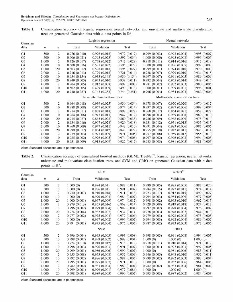
Table 1. Classification accuracy of logistic regression, neural networks, and univariate and multivariate classificationtrees on generated Gaussian data with n data points in �d.
Logistic regression Neural networksGaussiandata n d Train Validation Test Train Validation Test
G1 500 2 0.976 (0.010) 0.976 (0.012) 0.972 (0.017) 0.999 (0.003) 0.993 (0.004) 0.995 (0.007)G2 500 10 0.606 (0.021) 0.595 (0.025) 0.592 (0.034) 1.000 (0.000) 0.995 (0.008) 0.996 (0.005)G3 1�000 2 0.726 (0.017) 0.738 (0.022) 0.742 (0.028) 0.918 (0.011) 0.914 (0.016) 0.912 (0.018)G4 1�000 10 0.608 (0.016) 0.591 (0.022) 0.595 (0.029) 1.000 (0.000) 0.996 (0.005) 0.992 (0.009)G5 1�000 20 0.603 (0.012) 0.598 (0.018) 0.595 (0.027) 0.999 (0.001) 0.974 (0.010) 0.970 (0.009)G6 2�000 2 0.716 (0.013) 0.729 (0.018) 0.721 (0.014) 0.928 (0.007) 0.929 (0.010) 0.934 (0.015)G7 2�000 10 0.934 (0.154) 0.933 (0.148) 0.930 (0.154) 0.997 (0.007) 0.991 (0.005) 0.989 (0.009)G8 2�000 20 0.949 (0.005) 0.943 (0.010) 0.938 (0.011) 0.992 (0.004) 0.955 (0.014) 0.949 (0.015)G9 4�000 2 0.904 (0.005) 0.912 (0.008) 0.899 (0.008) 0.981 (0.002) 0.982 (0.003) 0.980 (0.005)G10 4�000 10 0.502 (0.005) 0.499 (0.009) 0.499 (0.013) 1.000 (0.001) 0.999 (0.001) 0.998 (0.001)G11 4�000 20 0.740 (0.257) 0.743 (0.253) 0.744 (0.251) 0.996 (0.003) 0.984 (0.003) 0.982 (0.006)
Univariate classification trees Multivariate classification trees
G1 500 2 0.964 (0.018) 0.939 (0.025) 0.930 (0.054) 0.978 (0.007) 0.970 (0.020) 0.970 (0.012)G2 500 10 0.988 (0.008) 0.967 (0.009) 0.974 (0.014) 0.997 (0.002) 0.997 (0.006) 0.998 (0.004)G3 1�000 2 0.914 (0.011) 0.888 (0.018) 0.892 (0.022) 0.868 (0.017) 0.854 (0.021) 0.857 (0.022)G4 1�000 10 0.964 (0.006) 0.947 (0.013) 0.947 (0.012) 0.998 (0.003) 0.989 (0.008) 0.989 (0.010)G5 1�000 20 0.915 (0.027) 0.865 (0.028) 0.860 (0.033) 0.986 (0.009) 0.968 (0.009) 0.975 (0.014)G6 2�000 2 0.934 (0.016) 0.907 (0.028) 0.920 (0.018) 0.931 (0.012) 0.931 (0.013) 0.935 (0.013)G7 2�000 10 0.960 (0.009) 0.947 (0.011) 0.943 (0.010) 0.991 (0.004) 0.983 (0.006) 0.987 (0.006)G8 2�000 20 0.899 (0.012) 0.854 (0.012) 0.848 (0.022) 0.955 (0.010) 0.942 (0.011) 0.945 (0.014)G9 4�000 2 0.979 (0.003) 0.973 (0.009) 0.971 (0.005) 0.957 (0.008) 0.959 (0.012) 0.955 (0.010)G10 4�000 10 0.985 (0.002) 0.976 (0.005) 0.974 (0.006) 0.997 (0.002) 0.996 (0.003) 0.994 (0.003)G11 4�000 20 0.951 (0.009) 0.918 (0.009) 0.922 (0.012) 0.983 (0.003) 0.981 (0.005) 0.981 (0.005)
Note. Standard deviations are in parentheses.
Table 2. Classification accuracy of generalized boosted methods (GBM), TreeNet™, logistic regression, neural networks,univariate and multivariate classification trees, and SVM and CRIO on generated Gaussian data with n datapoints in �d.
GBM TreeNet™Gaussiandata n d Train Validation Test Train Validation Test
G1 500 2 1000 (0) 0984 (0.01) 0987 (0.011) 0990 (0.005) 0985 (0.005) 0982 (0.020)G2 500 10 1000 (0) 0986 (0.01) 0991 (0.007) 0984 (0.015) 0977 (0.011) 0974 (0.014)G3 1�000 2 0930 (0.007) 0910 (0.018) 0911 (0.018) 0923 (0.017) 0912 (0.015) 0899 (0.027)G4 1�000 10 1000 (0) 0990 (0.004) 0984 (0.007) 0994 (0.003) 0984 (0.009) 0977 (0.008)G5 1�000 20 1000 (0.001) 0967 (0.009) 097 (0.012) 0998 (0.002) 0963 (0.010) 0962 (0.015)G6 2�000 2 0879 (0.013) 0865 (0.016) 0868 (0.014) 0929 (0.008) 0919 (0.018) 0924 (0.012)G7 2�000 10 0996 (0.002) 0979 (0.004) 0982 (0.004) 0992 (0.002) 0978 (0.004) 0976 (0.007)G8 2�000 20 0974 (0.004) 0932 (0.007) 0934 (0.01) 0978 (0.003) 0948 (0.007) 0944 (0.013)G9 4�000 2 0977 (0.002) 0975 (0.004) 0972 (0.004) 0979 (0.003) 0978 (0.003) 0973 (0.005)G10 4�000 10 1000 (0) 0997 (0.002) 0996 (0.002) 0994 (0.003) 0992 (0.004) 0989 (0.007)G11 4�000 20 099 (0.001) 0975 (0.004) 0976 (0.005) 0987 (0.002) 0973 (0.003) 0972 (0.006)
SVM CRIO
G1 500 2 0996 (0.004) 0993 (0.003) 0993 (0.008) 0998 (0.003) 0991 (0.008) 0994 (0.005)G2 500 10 0998 (0.002) 0999 (0.002) 0998 (0.004) 1000 (0) 1000 (0) 1000 (0)G3 1�000 2 0924 (0.010) 0918 (0.012) 0915 (0.018) 0918 (0.011) 0910 (0.014) 0921 (0.019)G4 1�000 10 0998 (0.003) 0996 (0.003) 0991 (0.007) 1000 (0.001) 0997 (0.003) 0997 (0.005)G5 1�000 20 0999 (0.001) 0986 (0.006) 0990 (0.007) 1000 (0) 0981 (0.006) 0985 (0.011)G6 2�000 2 0955 (0.008) 0953 (0.008) 0952 (0.009) 0946 (0.005) 0948 (0.010) 0952 (0.011)G7 2�000 10 0992 (0.002) 0986 (0.003) 0987 (0.005) 0999 (0.002) 0992 (0.003) 0993 (0.004)G8 2�000 20 0995 (0.001) 0975 (0.007) 0971 (0.010) 1000 (0) 0962 (0.006) 0964 (0.005)G9 4�000 2 0982 (0.002) 0983 (0.004) 0980 (0.004) 0982 (0.002) 0983 (0.004) 0981 (0.004)G10 4�000 10 0999 (0.001) 0999 (0.001) 0972 (0.084) 1000 (0) 1000 (0) 1000 (0)G11 4�000 20 0998 (0.001) 0989 (0.003) 0990 (0.002) 0993 (0.003) 0987 (0.002) 0984 (0.003)
Note. Standard deviations are in parentheses.
Bertsimas and Shioda: Classification and Regression via Integer Optimization264 Operations Research 55(2), pp. 252–271, © 2007 INFORMS
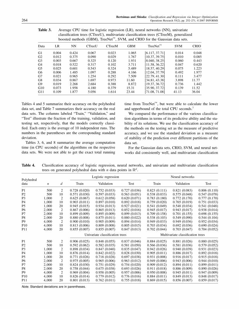
Table 3. Average CPU time for logistic regression (LR), neural networks (NN), univariateclassification trees (CTreeU), multivariate classification trees (CTreeM), generalizedboosted methods (GBM), TreeNet™, SVM, and CRIO for the Gaussian data sets.
Data LR NN CTreeU CTreeM GBM TreeNet™ SVM CRIO
G1 0.004 0.424 0.067 0.023 1065 +6117�3771, 0014 0048G2 0.012 0.375 0.090 0.029 1767 +1037�3975, 0010 0085G3 0.003 0.667 0.325 0.120 1931 +8040�3825, 0060 0443G4 0.018 0.522 0.317 0.102 3711 +1158�3622, 0047 0620G5 0.025 0.601 0.543 0.324 5489 +1857�4029, 0075 1223G6 0.006 1.485 1.097 0.288 4166 +1204�3779, 0492 1977G7 0.021 0.965 1.254 0.292 7509 +2279�4130, 0111 3477G8 0.034 0.867 1.697 0.973 1160 +3481�4338, 3898 1177G9 0.019 2.268 2.684 0.388 8872 +1937�3672, 0736 1442G10 0.073 1.958 4.180 0.379 1531 +3590�3772, 0139 1152G11 0.109 1.877 5.056 1.614 2344 +7108�7108, 4113 3604
Tables 4 and 5 summarize their accuracy on the polyhedraldata set, and Table 7 summarizes their accuracy on the realdata sets. The columns labeled “Train,” “Validation,” and“Test” illustrate the fraction of the training, validation, andtesting set, respectively, that the models correctly classi-fied. Each entry is the average of 10 independent runs. Thenumbers in the parentheses are the corresponding standarddeviation.Tables 3, 6, and 8 summarize the average computation
time (in CPU seconds) of the algorithms on the respectivedata sets. We were not able to get the exact total running
Table 4. Classification accuracy of logistic regression, neural networks, and univariate and multivariate classificationtrees on generated polyhedral data with n data points in �d.
Logistic regression Neural networksPolyhedraldata n d Train Validation Test Train Validation Test
P1 500 2 0728 (0.020) 0752 (0.033) 0727 (0.036) 0823 (0.111) 0821 (0.083) 0806 (0.110)P2 500 10 0571 (0.030) 0597 (0.033) 0563 (0.051) 0538 (0.033) 0575 (0.048) 0547 (0.078)P3 1�000 2 0625 (0.067) 0612 (0.058) 0620 (0.071) 0783 (0.180) 0772 (0.170) 0777 (0.170)P4 1�000 10 0903 (0.011) 0897 (0.010) 0892 (0.018) 0759 (0.020) 0765 (0.019) 0751 (0.033)P5 1�000 20 0945 (0.015) 0934 (0.013) 0927 (0.021) 0541 (0.049) 0548 (0.034) 0541 (0.048)P6 2�000 2 0867 (0.006) 0865 (0.013) 0852 (0.016) 0945 (0.017) 0943 (0.017) 0938 (0.014)P7 2�000 10 0899 (0.009) 0895 (0.009) 0899 (0.013) 0709 (0.158) 0701 (0.155) 0698 (0.155)P8 2�000 20 0880 (0.008) 0875 (0.011) 0880 (0.022) 0538 (0.103) 0549 (0.090) 0544 (0.104)P9 4�000 2 0900 (0.010) 0905 (0.009) 0894 (0.014) 0949 (0.033) 0949 (0.036) 0952 (0.034)P10 4�000 10 0813 (0.006) 0809 (0.008) 0805 (0.015) 0703 (0.034) 0692 (0.036) 0690 (0.024)P11 4�000 20 0855 (0.007) 0855 (0.007) 0847 (0.013) 0702 (0.044) 0703 (0.047) 0704 (0.052)
Univariate classification trees Multivariate classification trees
P1 500 2 0906 (0.025) 0848 (0.055) 0837 (0.046) 0884 (0.025) 0881 (0.026) 0880 (0.025)P2 500 10 0592 (0.062) 0582 (0.035) 0581 (0.050) 0566 (0.036) 0581 (0.036) 0579 (0.052)P3 1�000 2 0898 (0.034) 0847 (0.040) 0835 (0.047) 0942 (0.026) 0940 (0.039) 0931 (0.023)P4 1�000 10 0876 (0.014) 0842 (0.022) 0828 (0.030) 0905 (0.011) 0886 (0.017) 0892 (0.018)P5 1�000 20 0771 (0.026) 0718 (0.028) 0697 (0.038) 0931 (0.008) 0916 (0.017) 0915 (0.018)P6 2�000 2 0975 (0.005) 0965 (0.006) 0963 (0.012) 0949 (0.006) 0943 (0.006) 0944 (0.010)P7 2�000 10 0824 (0.030) 0751 (0.029) 0754 (0.020) 0909 (0.012) 0894 (0.011) 0899 (0.011)P8 2�000 20 0758 (0.044) 0675 (0.038) 0693 (0.026) 0911 (0.018) 0886 (0.009) 0890 (0.026)P9 4�000 2 0969 (0.004) 0958 (0.005) 0957 (0.006) 0950 (0.008) 0945 (0.011) 0947 (0.009)P10 4�000 10 0826 (0.014) 0779 (0.012) 0776 (0.016) 0884 (0.011) 0849 (0.013) 0848 (0.017)P11 4�000 20 0801 (0.013) 0762 (0.011) 0755 (0.018) 0869 (0.015) 0856 (0.007) 0859 (0.017)
Note. Standard deviations are in parentheses.
time from TreeNet™, but were able to calculate the lowerand upperbound of the total CPU seconds.7
We compared the performance of the various classifica-tion algorithms in terms of its predictive ability and the sta-bility of its solutions. We use the classification accuracy ofthe methods on the testing set as the measure of predictiveaccuracy, and we use the standard deviation as a measureof stability of the prediction over different partitions of thedata set.For the Gaussian data sets, CRIO, SVM, and neural net-
works did consistently well, and multivariate classification
Bertsimas and Shioda: Classification and Regression via Integer OptimizationOperations Research 55(2), pp. 252–271, © 2007 INFORMS 265
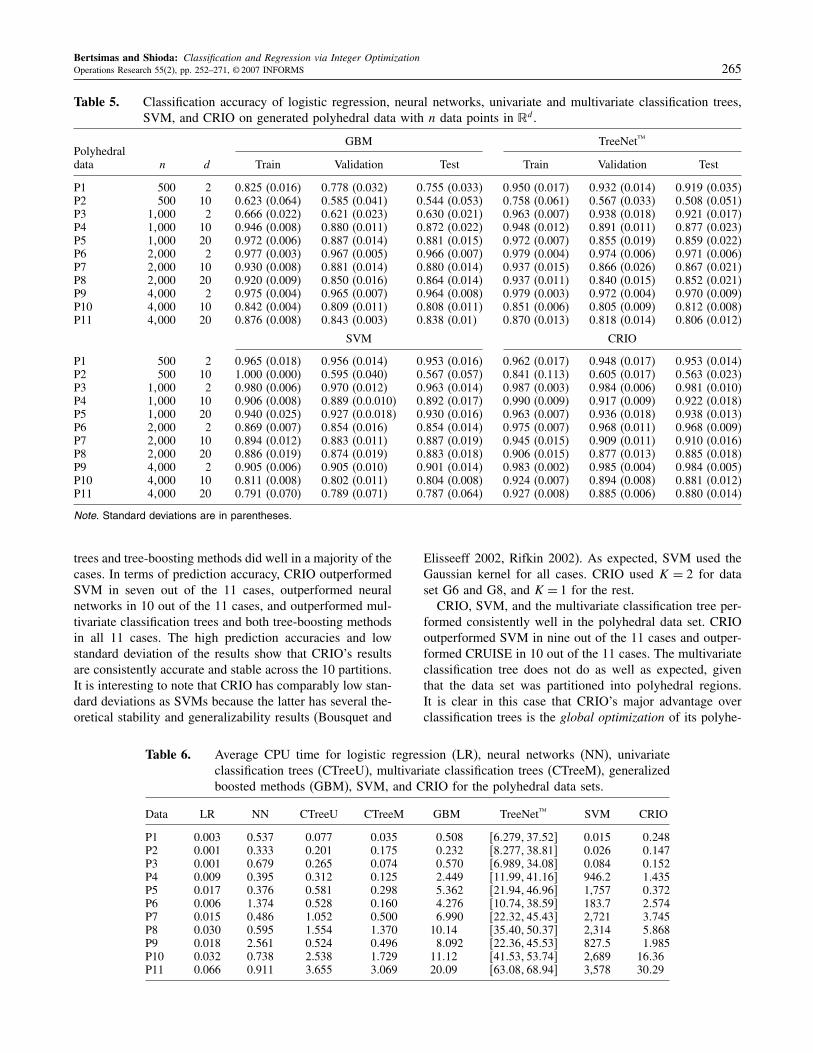
Table 5. Classification accuracy of logistic regression, neural networks, univariate and multivariate classification trees,SVM, and CRIO on generated polyhedral data with n data points in �d.
GBM TreeNet™Polyhedraldata n d Train Validation Test Train Validation Test
P1 500 2 0825 (0.016) 0778 (0.032) 0755 (0.033) 0950 (0.017) 0932 (0.014) 0919 (0.035)P2 500 10 0623 (0.064) 0585 (0.041) 0544 (0.053) 0758 (0.061) 0567 (0.033) 0508 (0.051)P3 1�000 2 0666 (0.022) 0621 (0.023) 0630 (0.021) 0963 (0.007) 0938 (0.018) 0921 (0.017)P4 1�000 10 0946 (0.008) 0880 (0.011) 0872 (0.022) 0948 (0.012) 0891 (0.011) 0877 (0.023)P5 1�000 20 0972 (0.006) 0887 (0.014) 0881 (0.015) 0972 (0.007) 0855 (0.019) 0859 (0.022)P6 2�000 2 0977 (0.003) 0967 (0.005) 0966 (0.007) 0979 (0.004) 0974 (0.006) 0971 (0.006)P7 2�000 10 0930 (0.008) 0881 (0.014) 0880 (0.014) 0937 (0.015) 0866 (0.026) 0867 (0.021)P8 2�000 20 0920 (0.009) 0850 (0.016) 0864 (0.014) 0937 (0.011) 0840 (0.015) 0852 (0.021)P9 4�000 2 0975 (0.004) 0965 (0.007) 0964 (0.008) 0979 (0.003) 0972 (0.004) 0970 (0.009)P10 4�000 10 0842 (0.004) 0809 (0.011) 0808 (0.011) 0851 (0.006) 0805 (0.009) 0812 (0.008)P11 4�000 20 0876 (0.008) 0843 (0.003) 0838 (0.01) 0870 (0.013) 0818 (0.014) 0806 (0.012)
SVM CRIO
P1 500 2 0965 (0.018) 0956 (0.014) 0953 (0.016) 0962 (0.017) 0948 (0.017) 0953 (0.014)P2 500 10 1000 (0.000) 0595 (0.040) 0567 (0.057) 0841 (0.113) 0605 (0.017) 0563 (0.023)P3 1�000 2 0980 (0.006) 0970 (0.012) 0963 (0.014) 0987 (0.003) 0984 (0.006) 0981 (0.010)P4 1�000 10 0906 (0.008) 0889 (0.0.010) 0892 (0.017) 0990 (0.009) 0917 (0.009) 0922 (0.018)P5 1�000 20 0940 (0.025) 0927 (0.0.018) 0930 (0.016) 0963 (0.007) 0936 (0.018) 0938 (0.013)P6 2�000 2 0869 (0.007) 0854 (0.016) 0854 (0.014) 0975 (0.007) 0968 (0.011) 0968 (0.009)P7 2�000 10 0894 (0.012) 0883 (0.011) 0887 (0.019) 0945 (0.015) 0909 (0.011) 0910 (0.016)P8 2�000 20 0886 (0.019) 0874 (0.019) 0883 (0.018) 0906 (0.015) 0877 (0.013) 0885 (0.018)P9 4�000 2 0905 (0.006) 0905 (0.010) 0901 (0.014) 0983 (0.002) 0985 (0.004) 0984 (0.005)P10 4�000 10 0811 (0.008) 0802 (0.011) 0804 (0.008) 0924 (0.007) 0894 (0.008) 0881 (0.012)P11 4�000 20 0791 (0.070) 0789 (0.071) 0787 (0.064) 0927 (0.008) 0885 (0.006) 0880 (0.014)
Note. Standard deviations are in parentheses.
trees and tree-boosting methods did well in a majority of thecases. In terms of prediction accuracy, CRIO outperformedSVM in seven out of the 11 cases, outperformed neuralnetworks in 10 out of the 11 cases, and outperformed mul-tivariate classification trees and both tree-boosting methodsin all 11 cases. The high prediction accuracies and lowstandard deviation of the results show that CRIO’s resultsare consistently accurate and stable across the 10 partitions.It is interesting to note that CRIO has comparably low stan-dard deviations as SVMs because the latter has several the-oretical stability and generalizability results (Bousquet and
Table 6. Average CPU time for logistic regression (LR), neural networks (NN), univariateclassification trees (CTreeU), multivariate classification trees (CTreeM), generalizedboosted methods (GBM), SVM, and CRIO for the polyhedral data sets.
Data LR NN CTreeU CTreeM GBM TreeNet™ SVM CRIO
P1 0.003 0.537 0.077 0.035 0508 +6279�3752, 0.015 0248P2 0.001 0.333 0.201 0.175 0232 +8277�3881, 0.026 0147P3 0.001 0.679 0.265 0.074 0570 +6989�3408, 0.084 0152P4 0.009 0.395 0.312 0.125 2449 +1199�4116, 946.2 1435P5 0.017 0.376 0.581 0.298 5362 +2194�4696, 1,757 0372P6 0.006 1.374 0.528 0.160 4276 +1074�3859, 183.7 2574P7 0.015 0.486 1.052 0.500 6990 +2232�4543, 2,721 3745P8 0.030 0.595 1.554 1.370 1014 +3540�5037, 2,314 5868P9 0.018 2.561 0.524 0.496 8092 +2236�4553, 827.5 1985P10 0.032 0.738 2.538 1.729 1112 +4153�5374, 2,689 1636P11 0.066 0.911 3.655 3.069 2009 +6308�6894, 3,578 3029
Elisseeff 2002, Rifkin 2002). As expected, SVM used theGaussian kernel for all cases. CRIO used K = 2 for dataset G6 and G8, and K = 1 for the rest.CRIO, SVM, and the multivariate classification tree per-
formed consistently well in the polyhedral data set. CRIOoutperformed SVM in nine out of the 11 cases and outper-formed CRUISE in 10 out of the 11 cases. The multivariateclassification tree does not do as well as expected, giventhat the data set was partitioned into polyhedral regions.It is clear in this case that CRIO’s major advantage overclassification trees is the global optimization of its polyhe-
Bertsimas and Shioda: Classification and Regression via Integer Optimization266 Operations Research 55(2), pp. 252–271, © 2007 INFORMS
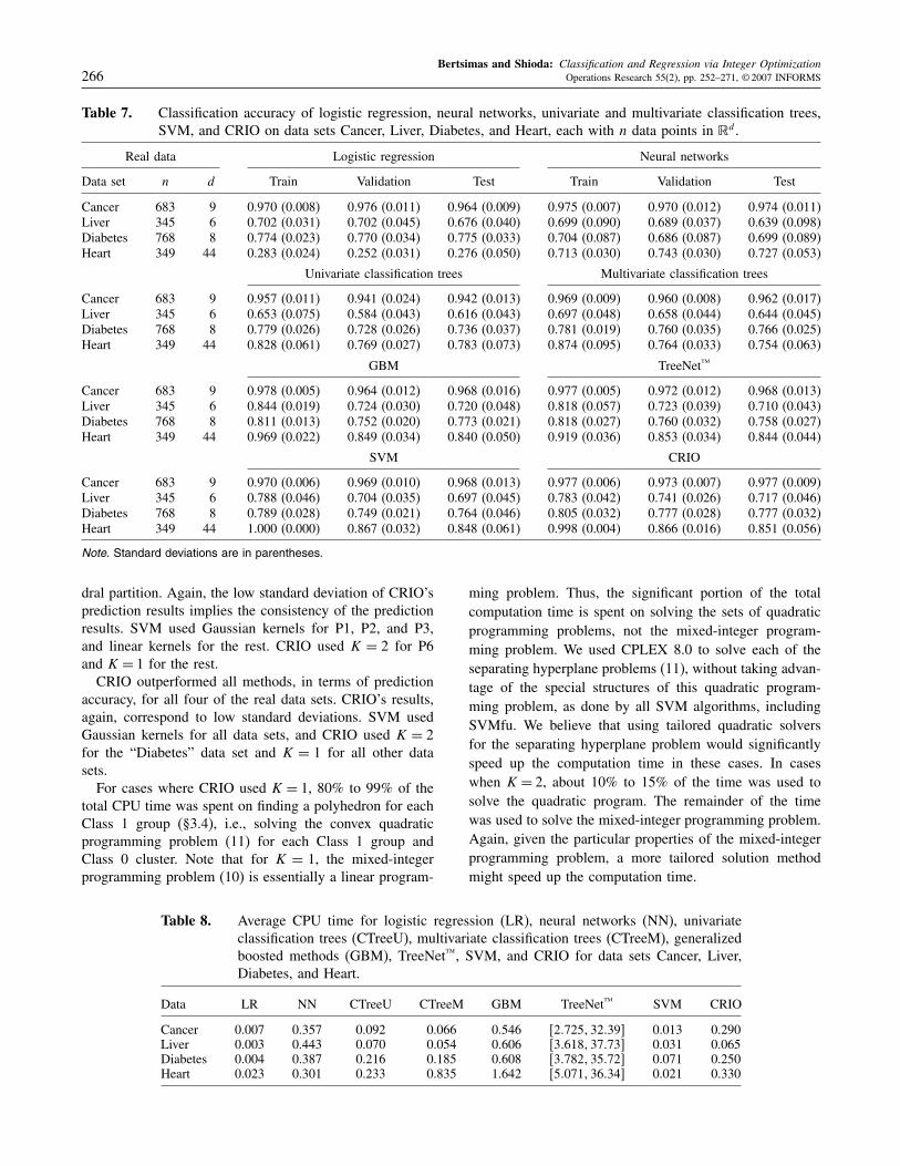
Table 7. Classification accuracy of logistic regression, neural networks, univariate and multivariate classification trees,SVM, and CRIO on data sets Cancer, Liver, Diabetes, and Heart, each with n data points in �d.
Real data Logistic regression Neural networks
Data set n d Train Validation Test Train Validation Test
Cancer 683 9 0.970 (0.008) 0.976 (0.011) 0.964 (0.009) 0.975 (0.007) 0.970 (0.012) 0.974 (0.011)Liver 345 6 0.702 (0.031) 0.702 (0.045) 0.676 (0.040) 0.699 (0.090) 0.689 (0.037) 0.639 (0.098)Diabetes 768 8 0.774 (0.023) 0.770 (0.034) 0.775 (0.033) 0.704 (0.087) 0.686 (0.087) 0.699 (0.089)Heart 349 44 0.283 (0.024) 0.252 (0.031) 0.276 (0.050) 0.713 (0.030) 0.743 (0.030) 0.727 (0.053)
Univariate classification trees Multivariate classification trees
Cancer 683 9 0.957 (0.011) 0.941 (0.024) 0.942 (0.013) 0.969 (0.009) 0.960 (0.008) 0.962 (0.017)Liver 345 6 0.653 (0.075) 0.584 (0.043) 0.616 (0.043) 0.697 (0.048) 0.658 (0.044) 0.644 (0.045)Diabetes 768 8 0.779 (0.026) 0.728 (0.026) 0.736 (0.037) 0.781 (0.019) 0.760 (0.035) 0.766 (0.025)Heart 349 44 0.828 (0.061) 0.769 (0.027) 0.783 (0.073) 0.874 (0.095) 0.764 (0.033) 0.754 (0.063)
GBM TreeNet™
Cancer 683 9 0.978 (0.005) 0.964 (0.012) 0.968 (0.016) 0.977 (0.005) 0.972 (0.012) 0.968 (0.013)Liver 345 6 0.844 (0.019) 0.724 (0.030) 0.720 (0.048) 0.818 (0.057) 0.723 (0.039) 0.710 (0.043)Diabetes 768 8 0.811 (0.013) 0.752 (0.020) 0.773 (0.021) 0.818 (0.027) 0.760 (0.032) 0.758 (0.027)Heart 349 44 0.969 (0.022) 0.849 (0.034) 0.840 (0.050) 0.919 (0.036) 0.853 (0.034) 0.844 (0.044)
SVM CRIO
Cancer 683 9 0.970 (0.006) 0.969 (0.010) 0.968 (0.013) 0.977 (0.006) 0.973 (0.007) 0.977 (0.009)Liver 345 6 0.788 (0.046) 0.704 (0.035) 0.697 (0.045) 0.783 (0.042) 0.741 (0.026) 0.717 (0.046)Diabetes 768 8 0.789 (0.028) 0.749 (0.021) 0.764 (0.046) 0.805 (0.032) 0.777 (0.028) 0.777 (0.032)Heart 349 44 1.000 (0.000) 0.867 (0.032) 0.848 (0.061) 0.998 (0.004) 0.866 (0.016) 0.851 (0.056)
Note. Standard deviations are in parentheses.
dral partition. Again, the low standard deviation of CRIO’sprediction results implies the consistency of the predictionresults. SVM used Gaussian kernels for P1, P2, and P3,and linear kernels for the rest. CRIO used K = 2 for P6and K = 1 for the rest.CRIO outperformed all methods, in terms of prediction
accuracy, for all four of the real data sets. CRIO’s results,again, correspond to low standard deviations. SVM usedGaussian kernels for all data sets, and CRIO used K = 2for the “Diabetes” data set and K = 1 for all other datasets.For cases where CRIO used K = 1, 80% to 99% of the
total CPU time was spent on finding a polyhedron for eachClass 1 group (§3.4), i.e., solving the convex quadraticprogramming problem (11) for each Class 1 group andClass 0 cluster. Note that for K = 1, the mixed-integerprogramming problem (10) is essentially a linear program-
Table 8. Average CPU time for logistic regression (LR), neural networks (NN), univariateclassification trees (CTreeU), multivariate classification trees (CTreeM), generalizedboosted methods (GBM), TreeNet™, SVM, and CRIO for data sets Cancer, Liver,Diabetes, and Heart.
Data LR NN CTreeU CTreeM GBM TreeNet™ SVM CRIO
Cancer 0.007 0.357 0.092 0.066 0.546 +2725�3239, 0.013 0.290Liver 0.003 0.443 0.070 0.054 0.606 +3618�3773, 0.031 0.065Diabetes 0.004 0.387 0.216 0.185 0.608 +3782�3572, 0.071 0.250Heart 0.023 0.301 0.233 0.835 1.642 +5071�3634, 0.021 0.330
ming problem. Thus, the significant portion of the totalcomputation time is spent on solving the sets of quadraticprogramming problems, not the mixed-integer program-ming problem. We used CPLEX 8.0 to solve each of theseparating hyperplane problems (11), without taking advan-tage of the special structures of this quadratic program-ming problem, as done by all SVM algorithms, includingSVMfu. We believe that using tailored quadratic solversfor the separating hyperplane problem would significantlyspeed up the computation time in these cases. In caseswhen K = 2, about 10% to 15% of the time was used tosolve the quadratic program. The remainder of the timewas used to solve the mixed-integer programming problem.Again, given the particular properties of the mixed-integerprogramming problem, a more tailored solution methodmight speed up the computation time.
Bertsimas and Shioda: Classification and Regression via Integer OptimizationOperations Research 55(2), pp. 252–271, © 2007 INFORMS 267
5.2. Regression Results
We tested the regression component of CRIO on three realdata sets found on the UCI data repository and Friedman’s(1999b) generated data set. We compared the results tolinear regression, neural networks with radial basis func-tions and generalized regression (via MATLAB’s® neu-ral networks toolbox), tree-boosting methods GBM andTreenet™ described in §5.1, and MARS (via R’s “poly-mars” package).Similar to the experiments on the classification data sets
in §5.1, each of the regression data was split into three parts,with 50%, 30%, and 20% of the data used for training, vali-dating, and testing, respectively. The assignment to each setwas done randomly, and the process was repeated 10 times.We used the validation set for CRIO to fine-tune the
value of parameter K. In all cases, we solved the mixed-integer programming problem (17) and set the parametersM , L, and ' to 10,000, 10, and 0.01, respectively. In neuralnetworks, we use the validation set to select the appropriatemodel (radial basis function versus generalized regression),adjust the number of epochs, the number of layers, thespread constant, and the accuracy parameter. For GBM andTreeNet™, we used the validation set to select the bestshrinkage value and maximum number of tree iterations.In MARS, we used the validation set to choose the appro-priate maximum number of basis functions and generalizedcross validation (gcv) value.
Regression Data. The “Boston” data, with 13 explana-tory variables and 506 observations, are the Boston housingdata set with the dependent variable being the median valueof houses in the suburbs of Boston. The “Abalone” data,with seven explanatory variables and 4,177 observations,attempt to predict the age of an abalone given its physiolog-ical measurements. The original “Abalone” data set had anadditional categorical input variable, but we omitted it forour experimentations because not all methods were capa-ble of treating such attributes. The “Auto” data, with fiveexplanatory variables and 392 observations, are the auto-mpg data set that determines the miles-per-gallon fuel con-sumption of an automobile, given the mechanical attributesof the car. The “Friedman” data set is a generated data setresulting from using a random function generating methodproposed by Friedman (1999b). All nine of the generateddata sets consist of 10 explanatory variables.
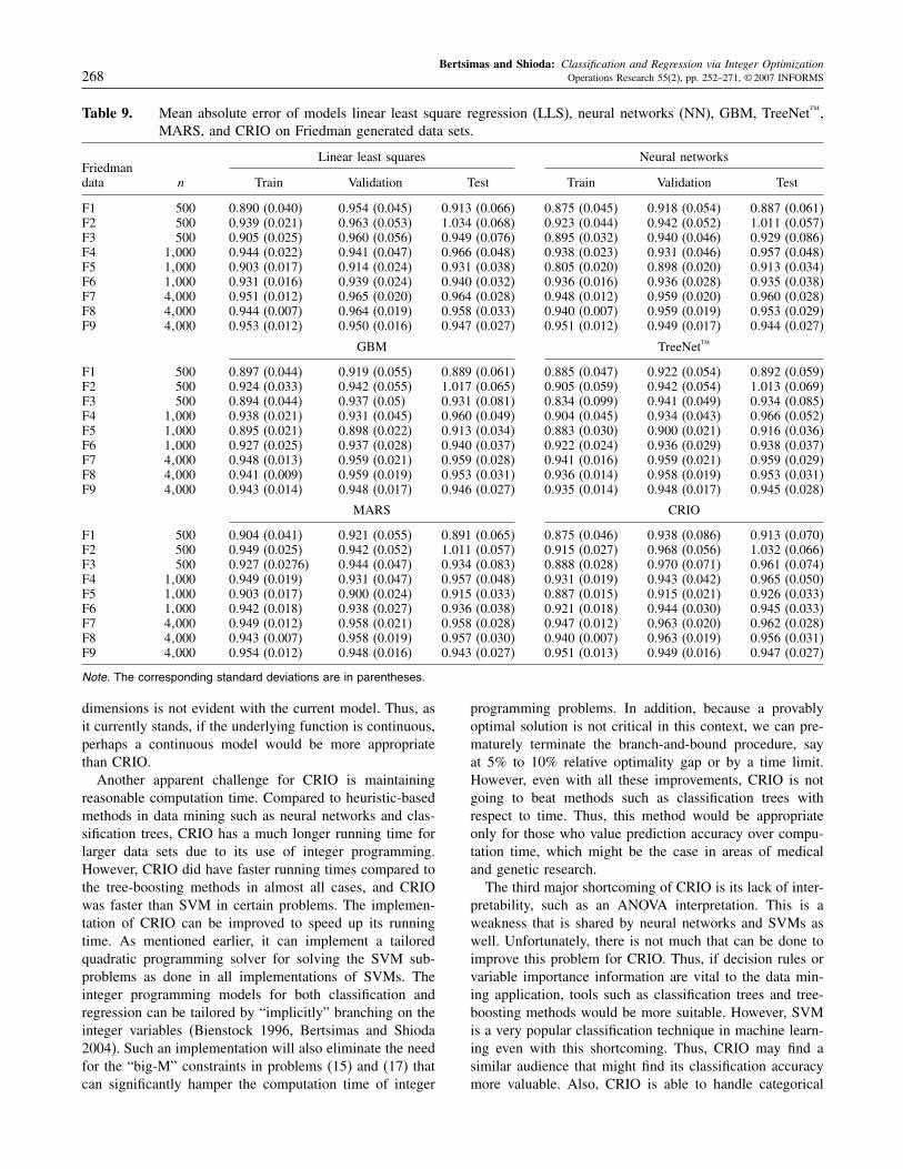
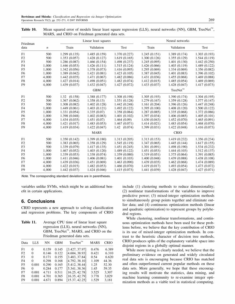
Results. Tables 9 and 10 illustrate the mean-absoluteerror and mean-squared error, respectively, of linear leastsquares regression (LLS), neural networks (NN), GBM,TreeNet™, MARS, and CRIO, averaged over the 10 randompartitions on the Friedman generated data sets. Tables 12and 13 illustrate the mean-absolute error and mean-squarederror, respectively, of the regression methods, averaged overthe 10 random partitions on the “Boston,” “Abalone,” and“Auto” data sets. The numbers in parentheses are the cor-responding standard deviations. Tables 11 and 14 illustratethe average running time, in terms of CPU seconds, of the
methods for the Friedman generated data sets and the realdata sets, respectively. Again, for TreeNet™, the lower andupper bounds of the total CPU seconds are shown becauseit does not currently report the exact total running time.As in the classification case, we measure the perfor-
mance of the various regression methods by their predic-tive ability and stability of their solutions. We measurethe prediction accuracy using both mean-absolute errorsand mean-squared errors between the predicted versus theactual response variable in the testing set, given that themean-absolute error is used as the goodness-of-fit criterionfor CRIO and mean-squared error is used as the goodness-of-fit criterion for linear least squares and the neural net-work model. GBM, TreeNet™, and MARS can be adjustedto deal with either loss criterion.CRIO used K = 2 for all data sets, neural networks
always used radial basis functions as the preferred modelwith just one layer of nodes, GBM used shrinkage value of001 and 3,000 tree iterations, and TreeNet™ used shrink-age of 001 and 4,000 tree iterations.Table 14 shows that CRIO has relatively reasonable aver-
age running time as the other methods for the smaller datasets, but its run time explodes for the larger “Abalone”data set. Unlike the classification component of CRIO, theregression component experiences a dramatic increase inrun time with larger data sets mainly due to the M param-eter in models (15) and (17). Because a tight estimate ofthis “big-M” parameter cannot be determined a priori, thelarge value of M seriously hampers the efficiency of theinteger programming solver.Clearly, the performance of the regression component
of CRIO is not as convincing as the classification com-ponent, and more testing and modifications are needed.Namely, we would need to make improvements to themodel (e.g., enforce continuity in the boundaries and findstronger approximations of the parameter M) and run morecomputational experiments before making any conclusions.
5.3. Discussion on Shortcomings
The computational experiments illustrated some benefitsand shortcomings of CRIO compared to other existingmethods in data mining and machine learning. The mainadvantage, at least in classification, is its prediction accu-racy and relative stability. However, there are many short-comings that need to be addressed.As mentioned in the previous section, the regression
component of CRIO clearly needs further development inits mathematical model and computational experimenta-tions. Its main weakness arises from the discontinuity of theregression line at the boundaries of the polyhedral regions.This is not the case of MARS, which maintains continu-ity of its regression function throughout the domain. Thus,CRIO’s predictive performance of general continuous func-tions are significantly hampered by this shortcoming, asseen with the Friedman data set. Continuity can be imposedby modifications to the mixed-integer programming prob-lem in the one-dimensional case, but the extension to higher
Bertsimas and Shioda: Classification and Regression via Integer Optimization268 Operations Research 55(2), pp. 252–271, © 2007 INFORMS
Table 9. Mean absolute error of models linear least square regression (LLS), neural networks (NN), GBM, TreeNet™,MARS, and CRIO on Friedman generated data sets.
Linear least squares Neural networksFriedmandata n Train Validation Test Train Validation Test
F1 500 0890 (0.040) 0954 (0.045) 0913 (0.066) 0875 (0.045) 0918 (0.054) 0887 (0.061)F2 500 0939 (0.021) 0963 (0.053) 1034 (0.068) 0923 (0.044) 0942 (0.052) 1011 (0.057)F3 500 0905 (0.025) 0960 (0.056) 0949 (0.076) 0895 (0.032) 0940 (0.046) 0929 (0.086)F4 1�000 0944 (0.022) 0941 (0.047) 0966 (0.048) 0938 (0.023) 0931 (0.046) 0957 (0.048)F5 1�000 0903 (0.017) 0914 (0.024) 0931 (0.038) 0805 (0.020) 0898 (0.020) 0913 (0.034)F6 1�000 0931 (0.016) 0939 (0.024) 0940 (0.032) 0936 (0.016) 0936 (0.028) 0935 (0.038)F7 4�000 0951 (0.012) 0965 (0.020) 0964 (0.028) 0948 (0.012) 0959 (0.020) 0960 (0.028)F8 4�000 0944 (0.007) 0964 (0.019) 0958 (0.033) 0940 (0.007) 0959 (0.019) 0953 (0.029)F9 4�000 0953 (0.012) 0950 (0.016) 0947 (0.027) 0951 (0.012) 0949 (0.017) 0944 (0.027)
GBM TreeNet™
F1 500 0897 (0.044) 0919 (0.055) 0889 (0.061) 0885 (0.047) 0922 (0.054) 0892 (0.059)F2 500 0924 (0.033) 0942 (0.055) 1017 (0.065) 0905 (0.059) 0942 (0.054) 1013 (0.069)F3 500 0894 (0.044) 0937 (0.05) 0931 (0.081) 0834 (0.099) 0941 (0.049) 0934 (0.085)F4 1�000 0938 (0.021) 0931 (0.045) 0960 (0.049) 0904 (0.045) 0934 (0.043) 0966 (0.052)F5 1�000 0895 (0.021) 0898 (0.022) 0913 (0.034) 0883 (0.030) 0900 (0.021) 0916 (0.036)F6 1�000 0927 (0.025) 0937 (0.028) 0940 (0.037) 0922 (0.024) 0936 (0.029) 0938 (0.037)F7 4�000 0948 (0.013) 0959 (0.021) 0959 (0.028) 0941 (0.016) 0959 (0.021) 0959 (0.029)F8 4�000 0941 (0.009) 0959 (0.019) 0953 (0.031) 0936 (0.014) 0958 (0.019) 0953 (0.031)F9 4�000 0943 (0.014) 0948 (0.017) 0946 (0.027) 0935 (0.014) 0948 (0.017) 0945 (0.028)
MARS CRIO
F1 500 0904 (0.041) 0921 (0.055) 0891 (0.065) 0875 (0.046) 0938 (0.086) 0913 (0.070)F2 500 0949 (0.025) 0942 (0.052) 1011 (0.057) 0915 (0.027) 0968 (0.056) 1032 (0.066)F3 500 0927 (0.0276) 0944 (0.047) 0934 (0.083) 0888 (0.028) 0970 (0.071) 0961 (0.074)F4 1�000 0949 (0.019) 0931 (0.047) 0957 (0.048) 0931 (0.019) 0943 (0.042) 0965 (0.050)F5 1�000 0903 (0.017) 0900 (0.024) 0915 (0.033) 0887 (0.015) 0915 (0.021) 0926 (0.033)F6 1�000 0942 (0.018) 0938 (0.027) 0936 (0.038) 0921 (0.018) 0944 (0.030) 0945 (0.033)F7 4�000 0949 (0.012) 0958 (0.021) 0958 (0.028) 0947 (0.012) 0963 (0.020) 0962 (0.028)F8 4�000 0943 (0.007) 0958 (0.019) 0957 (0.030) 0940 (0.007) 0963 (0.019) 0956 (0.031)F9 4�000 0954 (0.012) 0948 (0.016) 0943 (0.027) 0951 (0.013) 0949 (0.016) 0947 (0.027)
Note. The corresponding standard deviations are in parentheses.
dimensions is not evident with the current model. Thus, asit currently stands, if the underlying function is continuous,perhaps a continuous model would be more appropriatethan CRIO.Another apparent challenge for CRIO is maintaining
reasonable computation time. Compared to heuristic-basedmethods in data mining such as neural networks and clas-sification trees, CRIO has a much longer running time forlarger data sets due to its use of integer programming.However, CRIO did have faster running times compared tothe tree-boosting methods in almost all cases, and CRIOwas faster than SVM in certain problems. The implemen-tation of CRIO can be improved to speed up its runningtime. As mentioned earlier, it can implement a tailoredquadratic programming solver for solving the SVM sub-problems as done in all implementations of SVMs. Theinteger programming models for both classification andregression can be tailored by “implicitly” branching on theinteger variables (Bienstock 1996, Bertsimas and Shioda2004). Such an implementation will also eliminate the needfor the “big-M” constraints in problems (15) and (17) thatcan significantly hamper the computation time of integer
programming problems. In addition, because a provablyoptimal solution is not critical in this context, we can pre-maturely terminate the branch-and-bound procedure, sayat 5% to 10% relative optimality gap or by a time limit.However, even with all these improvements, CRIO is notgoing to beat methods such as classification trees withrespect to time. Thus, this method would be appropriateonly for those who value prediction accuracy over compu-tation time, which might be the case in areas of medicaland genetic research.The third major shortcoming of CRIO is its lack of inter-
pretability, such as an ANOVA interpretation. This is aweakness that is shared by neural networks and SVMs aswell. Unfortunately, there is not much that can be done toimprove this problem for CRIO. Thus, if decision rules orvariable importance information are vital to the data min-ing application, tools such as classification trees and tree-boosting methods would be more suitable. However, SVMis a very popular classification technique in machine learn-ing even with this shortcoming. Thus, CRIO may find asimilar audience that might find its classification accuracymore valuable. Also, CRIO is able to handle categorical
Bertsimas and Shioda: Classification and Regression via Integer OptimizationOperations Research 55(2), pp. 252–271, © 2007 INFORMS 269
Table 10. Mean squared error of models linear least square regression (LLS), neural networks (NN), GBM, TreeNet™,MARS, and CRIO on Friedman generated data sets.
Linear least squares Neural networksFriedmandata n Train Validation Test Train Validation Test
F1 500 1.299 (0.135) 1.485 (0.159) 1.370 (0.227) 1.245 (0.151) 1.389 (0.174) 1.303 (0.193)F2 500 1.353 (0.057) 1.428 (0.127) 1.619 (0.165) 1.300 (0.126) 1.355 (0.129) 1.544 (0.119)F3 500 1.286 (0.087) 1.466 (0.154) 1.498 (0.237) 1.245 (0.095) 1.401 (0.130) 1.442 (0.250)F4 1�000 1.446 (0.053) 1.426 (0.111) 1.515 (0.124) 1.426 (0.066) 1.403 (0.119) 1.489 (0.122)F5 1�000 1.342 (0.056) 1.378 (0.073) 1.416 (0.095) 1.295 (0.069) 1.334 (0.069) 1.356 (0.082)F6 1�000 1.389 (0.042) 1.421 (0.081) 1.423 (0.105) 1.387 (0.045) 1.401 (0.083) 1.396 (0.102)F7 4�000 1.442 (0.035) 1.471 (0.067) 1.482 (0.086) 1.431 (0.036) 1.455 (0.068) 1.469 (0.088)F8 4�000 1.427 (0.014) 1.498 (0.051) 1.482 (0.074) 1.412 (0.015) 1.485 (0.054) 1.469 (0.069)F9 4�000 1.439 (0.037) 1.432 (0.047) 1.427 (0.072) 1.433 (0.037) 1.428 (0.047) 1.417 (0.073)
GBM TreeNet™
F1 500 1.32 (0.158) 1.388 (0.177) 1.308 (0.198) 1.305 (0.193) 1.390 (0.174) 1.304 (0.195)F2 500 1.367 (0.062) 1.358 (0.13) 1.551 (0.128) 1.279 (0.167) 1.359 (0.128) 1.577 (0.147)F3 500 1.308 (0.082) 1.402 (0.128) 1.442 (0.248) 1.161 (0.204) 1.396 (0.126) 1.447 (0.248)F4 1�000 1.449 (0.061) 1.403 (0.121) 1.492 (0.122) 1.395 (0.100) 1.408 (0.120) 1.500 (0.122)F5 1�000 1.331 (0.054) 1.335 (0.07) 1.358 (0.084) 1.287 (0.085) 1.335 (0.068) 1.372 (0.086)F6 1�000 1.398 (0.048) 1.402 (0.083) 1.401 (0.102) 1.397 (0.034) 1.406 (0.085) 1.405 (0.101)F7 4�000 1.434 (0.035) 1.451 (0.07) 1.464 (0.09) 1.430 (0.043) 1.452 (0.070) 1.465 (0.091)F8 4�000 1.421 (0.017) 1.483 (0.053) 1.467 (0.071) 1.414 (0.021) 1.483 (0.054) 1.468 (0.070)F9 4�000 1.419 (0.034) 1.422 (0.047) 1.42 (0.074) 1.399 (0.031) 1.422 (0.048) 1.416 (0.073)
MARS CRIO
F1 500 1.350 (0.142) 1.399 (0.180) 1.313 (0.205) 1.313 (0.153) 1.419 (0.232) 1.356 (0.234)F2 500 1.383 (0.065) 1.358 (0.129) 1.545 (0.119) 1.347 (0.065) 1.445 (0.144) 1.617 (0.155)F3 500 1.339 (0.079) 1.417 (0.135) 1.451 (0.245) 1.301 (0.091) 1.498 (0.190) 1.534 (0.232)F4 1�000 1.467 (0.052) 1.403 (0.120) 1.489 (0.122) 1.451 (0.053) 1.444 (0.103) 1.512 (0.137)F5 1�000 1.339 (0.053) 1.338 (0.074) 1.359 (0.080) 1.319 (0.051) 1.375 (0.064) 1.391 (0.085)F6 1�000 1.411 (0.046) 1.406 (0.081) 1.401 (0.103) 1.400 (0.048) 1.439 (0.088) 1.438 (0.108)F7 4�000 1.439 (0.036) 1.451 (0.069) 1.463 (0.090) 1.439 (0.035) 1.462 (0.068) 1.474 (0.089)F8 4�000 1.422 (0.015) 1.482 (0.053) 1.466 (0.070) 1.419 (0.017) 1.493 (0.054) 1.473 (0.072)F9 4�000 1.442 (0.037) 1.424 (0.046) 1.415 (0.073) 1.441 (0.039) 1.428 (0.047) 1.427 (0.071)
Note. The corresponding standard deviations are in parentheses.
variables unlike SVMs, which might be an additional ben-efit in certain applications.
6. ConclusionsCRIO represents a new approach to solving classificationand regression problems. The key components of CRIO
Table 11. Average CPU time of linear least squareregression (LLS), neural networks (NN),GBM, TreeNet™, MARS, and CRIO on theFriedman generated data sets.
Data LLS NN GBM TreeNet™ MARS CRIO
F1 0 0.159 0.145 +3427�3797, 0476 6389F2 0 0.146 0.122 +4604�3893, 0421 6310F3 0 0.171 0.155 +3483�3784, 054 6620F4 0 0.298 0.168 +4792�3810, 1109 4436F5 0001 0.290 0.165 +5412�3844, 125 5230F6 0 0.284 0.177 +5341�3836, 145 5935F7 0001 4.711 0.511 +1625�4278, 3525 3,307F8 0001 4.701 0.365 +1635�4279, 3778 3,029F9 0001 4.671 0.894 +1537�4225, 1529 3,181
include (1) clustering methods to reduce dimensionality;(2) nonlinear transformations of the variables to improvepredictive power; (3) mixed-integer optimization methodsto simultaneously group points together and eliminate out-lier data; and (4) continuous optimization methods (linearand quadratic optimization) to represent groups by polyhe-dral regions.While clustering, nonlinear transformations, and contin-
uous optimization methods have been used for these prob-lems before, we believe that the key contribution of CRIOis its use of mixed-integer optimization methods. In con-trast to the heuristic character of decision tree methods,CRIO produces splits of the explanatory variable space intodisjoint regions in a globally optimal manner.While more testing is clearly needed, we believe that the
preliminary evidence on generated and widely circulatedreal data sets is encouraging because CRIO has matchedand often outperformed current popular methods on thesedata sets. More generally, we hope that these encourag-ing results will motivate the statistics, data mining, andmachine learning community to re-examine integer opti-mization methods as a viable tool in statistical computing.
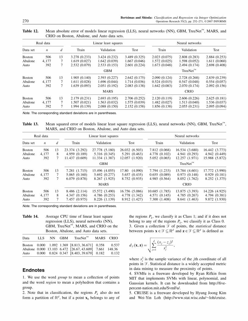
Bertsimas and Shioda: Classification and Regression via Integer Optimization270 Operations Research 55(2), pp. 252–271, © 2007 INFORMS
Table 12. Mean absolute error of models linear regression (LLS), neural networks (NN), GBM, TreeNet™, MARS, andCRIO on Boston, Abalone, and Auto data sets.
Real data Linear least squares Neural networks
Data set n d Train Validation Test Train Validation Test
Boston 506 13 3.278 (0.233) 3.424 (0.232) 3.489 (0.325) 2.023 (0.075) 2.808 (0.283) 2.884 (0.253)Abalone 4�177 7 1.619 (0.027) 1.642 (0.039) 1.667 (0.046) 1.572 (0.025) 1.598 (0.052) 1.611 (0.060)Auto 392 7 2.532 (0.079) 2.533 (0.153) 2.601 (0.224) 1.673 (0.048) 2.494 (0.174) 2.698 (0.408)
GBM TreeNet™
Boston 506 13 1.905 (0.140) 2.593 (0.227) 2.642 (0.175) 2.090 (0.124) 2.728 (0.268) 2.839 (0.239)Abalone 4�177 7 1.611 (0.028) 1.696 (0.044) 1.714 (0.036) 0.524 (0.015) 0.547 (0.048) 0.554 (0.057)Auto 392 7 1.639 (0.093) 2.051 (0.192) 2.083 (0.138) 1.642 (0.083) 2.070 (0.174) 2.092 (0.156)
MARS CRIO
Boston 506 13 2.179 (0.231) 2.693 (0.195) 2.706 (0.252) 2.120 (0.119) 2.606 (0.226) 2.625 (0.181)Abalone 4�177 7 1.507 (0.021) 1.563 (0.032) 1.575 (0.039) 1.482 (0.027) 1.513 (0.040) 1.536 (0.037)Auto 392 7 1.994 (0.139) 2.088 (0.150) 2.152 (0.158) 1.856 (0.138) 2.055 (0.231) 2.095 (0.094)
Note. The corresponding standard deviations are in parentheses.
Table 13. Mean squared error of models linear least square regression (LLS), neural networks (NN), GBM, TreeNet™,MARS, and CRIO on Boston, Abalone, and Auto data sets.
Real data Linear least squares Neural networks
Data set n d Train Validation Test Train Validation Test
Boston 506 13 23374 �3292� 27778 �5180� 26032 �6503� 7812 �0068� 16534 �3680� 16442 �3773�Abalone 4�177 8 4959 �0189� 5316 �0345� 5291 �0463� 4778 �0102� 4941 �0293� 4942 �0449�Auto 392 7 11437 �0609� 11334 �1387� 12057 �1920� 5052 �0065� 12257 �1971� 15988 �5872�
GBM TreeNet™
Boston 506 13 7281 �1715� 15496 �4055� 1780 �4090� 7794 �1233� 15784 �4601� 17772 �3990�Abalone 4�177 7 5065 �0160� 5692 �0277� 5657 �0435� 0655 �0089� 0973 �0148� 0929 �0181�Auto 392 7 6079 �0878� 8267 �1925� 8752 �0935� 4985 �0564� 8052 �1762� 8252 �1375�
MARS CRIO
Boston 506 13 8486 �2114� 15572 �3490� 16756 �5086� 10685 �1785� 13875 �3393� 14226 �4925�Abalone 4�177 8 4347 �0156� 4786 �0253� 4778 �1342� 4571 �0145� 4785 �0267� 4794 �0381�Auto 392 7 7457 �0975� 8226 �1139� 8912 �1427� 7300 �1408� 8641 �1463� 9872 �1930�
Note. The corresponding standard deviations are in parentheses.
Table 14. Average CPU time of linear least squareregression (LLS), neural networks (NN),GBM, TreeNet™, MARS, and CRIO on theBoston, Abalone, and Auto data sets.
Data LLS NN GBM TreeNet™ MARS CRIO
Boston 0.000 1092 1.369 +8813�36671, 0.358 0537Abalone 0.000 13103 6.472 +2667�43609, 7.661 14836Auto 0.000 0824 0.347 +8403�39679, 0.182 0132
Endnotes1. We use the word group to mean a collection of pointsand the word region to mean a polyhedron that contains agroup.2. Note that in classification, the regions Pk also do notform a partition of �d, but if a point x0 belongs to any of
the regions Pk, we classify it as Class 1; and if it does notbelong to any of the regions Pk, we classify it as Class 0.3. Given a collection � of points, the statistical distancebetween points x ∈� ⊆�d and z ∈� ⊆�d is defined as
d� �x� z�=√√√√ d∑
j=1
�xj − zj�2
s2j�
where s2j is the sample variance of the jth coordinate of allpoints in � . Statistical distance is a widely accepted metricin data mining to measure the proximity of points.4. SVMfu is a freeware developed by Ryan Rifkin fromMIT that implements SVMs with linear, polynomial, andGaussian kernels. It can be downloaded from http://five-percent-nation.mit.edu/SvmFu/.5. CRUISE is a freeware developed by Hyung Joong Kimand Wei-Yin Loh (http://www.stat.wisc.edu/∼loh/cruise.

Bertsimas and Shioda: Classification and Regression via Integer OptimizationOperations Research 55(2), pp. 252–271, © 2007 INFORMS 271
html). We also tested CART from Salford Systems, butCRUISE was comparable or outperformed the former inevery case. Thus, we present only the performance ofCRUISE in this paper.6. CPLEX 8.0 is a product of ILOG (http://www.ilog.com/products/cplex/).7. TreeNet™ reports the mean CPU seconds for every 10trees. Because only the first two decimal places are shown(often being 0.00), we could not compute the exact totalCPU seconds. However, we can clearly find the lower andupper bound of the total running time from this informa-tion.
AcknowledgmentsThe authors thank the referees for their recommendationsand guidance. The research of both authors was partiallysupported by the Singapore-MIT Alliance. In addition,R. Shioda was funded by the Discovery grant from NSERC.
ReferencesArthanari, T. S., Y. Dodge. 1993. Mathematical Programming in Statistics.
Wiley Classics Library Edition, Wiley–Interscience, New York.
Bennett, K. P., J. A. Blue. 1984. Optimal decision trees. R.P.I. Math Report214, Department of Mathematical Sciences, Rensselaer PolytechnicInstitute, Troy, NY.
Bertsimas, D., R. Shioda. 2004. An algorithm for cardinality constraintquadratic optimization. In review.
Bienstock, D. 1996. Computational study of families of mixed-integerquadratic programming problems. Math. Programming 74 121–140.
Bousquet, O., A. Elisseeff. 2002. Stability and generalization. J. MachineLearn. Res. 2 445–498.
Breiman, L., J. Friedman, R. Olshen, C. Stone. 1984. Classification andRegression Trees. Wadsworth International, Belmont, CA.
Friedman, J. 1991. Multivariate adaptive regression splines. Ann. Statist.19(1) 1–67.
Friedman, J. H. 1999a. Stochastic gradient boosting. http://www-stat.stanford.edu/˜jhf/ftp/stobst.ps.
Friedman, J. H. 1999b. Greedy function approximation: A gradient boost-ing machine. http://www-stat.stanford.edu/˜jhf/ftp/trebst.ps.
Friedman, J. H. 2002. Getting started with MART in R. http://www-stat.stanford.edu/˜jhf/r-mart/tutorial/tutorial.pdf.
Hastie, T., R. Tibshirani, J. Friedman. 2001. The Elements of StatisticalLearning. Springer-Verlag, New York.
ILOG CPLEX 7.1 Reference Guide. 2001. ILOG CPLEX Division, InclineVillage, NV.
Johnson, R. A., D. W. Wichern. 1998. Applied Multivariate StatisticalAnalysis, 4th ed. Prentice-Hall, Englewood Cliffs, NJ.
Kim, H., W. Y. Loh. 2000. CRUISE User Manual. Technical Report 989,Department of Statistics, University of Wisconsin, Madison, WI.
Kim, H., W. Y. Loh. 2001. Classification tree with unbiased multiwaysplits. J. Amer. Statist. Assoc. 96 598–604.
Loh, W. Y., Y. Shih. 1997. Split selection methods for classification trees.Statistica Sinica 7 815–840.
Mangasarian, O. L. 1965. Linear and nonlinear separation of patterns bylinear programming. Oper. Res. 13(3) 444–452.
Quinlan, R. 1993. C4.5: Programs for Machine Learning. Morgan Kauf-man, San Mateo, CA.
Ridgeway, G. 2005. Generalized boosted models: A guide to the gbmpackage. http://i-pensieri.com/gregr/papers/gbm-vignette.pdf.
Rifkin, R. 2002. Everything old is new again: A fresh look at historicalapproaches in machine learning. Ph.D. thesis, Electrical Engineeringand Comuter Science and Operations Research, Massachusetts Insti-tute of Technology, Cambridge, MA.
Rousseeuw, P. J., A. M. Leroy. 1987. Robust Regression and OutlierDetection. Wiley, New York.
Ryan, T. P. 1997. Modern Regression Methods. Wiley Series in Probabilityand Statistics, John Wiley & Sons, New York.
Vapnik, V. 1999. The Nature of Statistical Learning Theory. Springer-Verlag, New York.


![Dantzig Wolfe Decomposition - Université catholique … · Contents 1 Algorithm Description [Infanger, Bertsimas] 2 Examples [Bertsimas] 3 Application of Dantzig-Wolfe in Stochastic](https://img.pdfslide.us/doc/110x75/5b90f7ac09d3f2e6728d1f69/dantzig-wolfe-decomposition-universite-catholique-contents-1-algorithm-description.jpg)


![[1997 Bertsimas, Tsitsiklis] Introduction to Linear Optimization (Ch1-5)](https://img.pdfslide.us/doc/110x75/55cf96c0550346d0338d8e85/1997-bertsimas-tsitsiklis-introduction-to-linear-optimization-ch1-5.jpg)