Classical Yang-Mills theory

A. D. Boozera)

Department of Physics and Astronomy, University of New Mexico, Albuquerque, New Mexico 87131

(Received 14 October 2010; accepted 8 June 2011)

We consider classical Yang-Mills theory with point sources and derive equations of motion for the

coupled particle-field system. As an example, we discuss the special case of Yang-Mills theory

coupled to point particles in (1þ 1) dimensions. We formulate the initial value problem for the

system and describe several example solutions. VC 2011 American Association of Physics Teachers.

[DOI: 10.1119/1.3606478]

I. INTRODUCTION

Yang-Mills theory plays a central role in explaining fun-damental interactions, because both the strong and weakinteractions are described by Yang-Mills theories.1,2 Stu-dents are usually introduced to Yang-Mills theory in thecontext of quantum field theory and never encounter Yang-Mills theory in its classical form. In contrast, students donot study quantum electrodynamics until they have thor-oughly mastered classical electrodynamics. In this paper,we fill this gap by discussing classical Yang-Mills theorycoupled to point sources. We derive the equations of motionfor the coupled particle-field system and present severalexample solutions to these equations for Yang-Mills theoryin (1þ 1) dimensions.

In Sec. II, we briefly review ordinary classical electrody-namics. In Sec. III, we generalize ordinary electrodynamics towhat we call color electrodynamics, which can be thought ofas electrodynamics with three different types of charge. InSec. IV, we generalize from color electrodynamics to Yang-Mills theory by means of symmetry principles. We then spe-cialize to the case of (1þ 1) dimensions. In Sec. V, we discussordinary electrodynamics in (1þ 1) dimensions, and in Sec.VI, we discuss Yang-Mills theory in (1þ 1) dimensions. InSec. VII, we present several example solutions to the equa-tions of motion for Yang-Mills theory in (1þ 1) dimensions.

The following notation is used. The sign function �(x) isdefined such that �(x)¼ 1 if x> 0, �(x)¼ 0 if x¼ 0, and�(x)¼� 1 if x< 0. The step function h(x) is defined such thath(x)¼ 1 if x> 0, h(x)¼ 1/2 if x¼ 0, and h(x)¼ 0 if x< 0.

II. ORDINARY ELECTRODYNAMICS

We begin by briefly reviewing ordinary classical electro-dynamics. For simplicity, we consider the case of a singlepoint particle source. Let m and q denote the mass and elec-tric charge of the particle, and let zl(s) and wl(s)¼ dzl(s)/dsdenote its position and velocity at proper time s. The electro-magnetic field is described by a vector potential Al fromwhich we derive the field strength tensor Fl�:

Fl� ¼ @lA� � @�Al: (1)

The field strength tensor satisfies the field equation

@lFl� ¼ 4pJ�; (2)

where the current density Jl is given by3

JlðxÞ ¼ q

ðwlðsÞ dð4Þðx� zðsÞÞ ds: (3)

The particle equation of motion is

mdwl

ds¼ qFl�w�: (4)

Equations (1)–(4) give a complete description ofelectrodynamics.

An important property of electrodynamics is that it isinvariant under the transformation Al ! Alþ @lk, where kis an arbitrary position-dependent parameter. Such a trans-formation is called a local abelian gauge transformation:local, because k can be different at different points in space-time, and abelian, because the net effect of two such trans-formations is independent of the order in which they areperformed.

III. COLOR ELECTRODYNAMICS

We will now generalize electrodynamics so that instead ofone type of charge, electric charge, we have three types ofcharge, which we call color charge.4 We denote the threecolor charges of the particle by qx, qy, and qz, and we definea vector ~q � ðqx; qy; qzÞ, which we call the charge vector.Note that ~q is a vector in color space, not physical space. Wewill refer to vectors in color space as color vectors and willdenote them by using horizontal arrows.

In color electrodynamics there are three vector potentials,one for each type of color charge, which we collect to form acolor vector ~Al. The corresponding field strength tensor ~Fl�

is given by

~Fl� ¼ @l~A� � @�~Al: (5)

The field strength tensor satisfies the field equation

@l~Fl� ¼ 4p~J�; (6)

where the color current density ~Jl is given by

~JlðxÞ ¼ ~qð

wlðsÞ dð4Þðx� zðsÞÞ ds: (7)

The particle equation of motion is

mdwl

ds¼ ~q � ~Fl�w�: (8)

Equations (5)–(8) give a complete description of colorelectrodynamics.

The physical interpretation of color electrodynamics issimple: each type of color charge produces a corresponding

925 Am. J. Phys. 79 (9), September 2011 http://aapt.org/ajp VC 2011 American Association of Physics Teachers 925

color field that obeys the laws of ordinary electrodynamics,and charges and fields of different colors do not couple toeach other. The force on a particle is the sum of the forcesexerted by each of the three color fields.

Color electrodynamics is closely analogous to ordinaryelectrodynamics. For example, two particles with chargevectors ~q1 and ~q2 experience an attractive force if ~q1 �~q2 isnegative and a repulsive force if ~q1 �~q2 is positive. Also, thefield equation for the theory is linear and therefore obeys thesuperposition principle: the field generated by a collection ofparticles is the sum of the fields generated by the individualparticles.

Like ordinary electrodynamics, color electrodynamics isinvariant under local abelian gauge transformations, whichin this case take the form

~Al ! ~Al þ ~kl; (9)

where the color vector ~k is an arbitrary position-dependentparameter. But there is an additional symmetry of color elec-trodynamics that is not present in ordinary electrodynamics:we are free to globally rotate the color vectors. That is, thetheory is invariant under the transformation

~q! R~q; ~Jl ! R~Jl; (10)

~Al ! R~Al; ~Fl� ! R~Fl�; (11)

where R is an arbitrary rotation matrix.This rotational symmetry implies that the theory depends

only on the relative orientation of color vectors, not on theirabsolute orientation in color space. For example, we saw thatthe force between two particles depends only on the dotproduct ~q1 �~q2. Invariance under global color rotations isanalogous to invariance under Lorentz transformations,because a Lorentz-invariant theory depends only on relativevelocities, not on absolute velocities.

In what follows, it will be useful to restrict ourselves to in-finitesimal transformations. This restriction does not entail aloss of generality, because finite transformations can alwaysbe composed out of sequences of infinitesimal transforma-tions. Consider a rotation R of infinitesimal magnitude habout an axis n. For an arbitrary color vector~v, we have thatR~v ¼~vþ ~h�~v, where ~h � hn. From Eqs. (9)–(11), it fol-lows that color electrodynamics is invariant under thetransformation

~q! ~qþ ~h�~q; (12)

~Jl ! ~Jl þ ~h� ~Jl; (13)

~Al ! ~Al þ ~h� ~Al þ @l~k; (14)

~Fl� ! ~Fl� þ ~h� ~Fl�; (15)

where ~k and ~h are infinitesimal color vectors. The color vec-tor ~h must be constant, but ~k can be different at differentpoints in spacetime. We will refer to this transformation,which combines a local abelian gauge transformation with aglobal color rotation, as a general transformation.

IV. YANG-MILLS THEORY

Color electrodynamics is invariant under local abeliangauge transformations and global color rotations. We will

now generalize color electrodynamics so that it is invariantnot just under global color rotations, but local color rotationsas well; that is, we want our theory to be invariant under gen-eral transformations for which both ~k and ~h depend onposition.

We first introduce some terminology: a color vector ~v thattransforms like ~v!~vþ ~h�~v under a general transforma-tion is said to transform properly. So ~q, ~Jl, and ~Fl� shouldtransform properly, but ~Al should not. Our first task is to findan expression for the field strength tensor that transformsproperly, given Eq. (14) for the transformation of the vectorpotential. We want to generalize color electrodynamics, sowe start by considering the tensor

~Fl�0 � @l~A� � @�~Al: (16)

From Eqs. (14) and (16), it follows that

~Fl�0 ! ~Fl�

0 þ ~h� ~Fl�0 þ @l~h� ~A� � @�~h� ~Al; (17)

so ~Fl�0 does not transform properly. Another natural tensor to

consider is

~Fl�1 � g~Al � ~A�; (18)

where g is a constant with units of inverse charge. From Eqs.(14) and (18), it follows that

~Fl�1 ! ~Fl�

1 þ ~h� ~Fl�1 þ g@l~k� ~A� þ g~Al � @�~k; (19)

so ~Fl�1 does not transform properly either.5 In fact it is not

possible to define a viable field strength tensor if ~h and ~k aretaken to be independent parameters. But if we define

~Fl� � ~Fl�0 þ ~Fl�

1 ¼ @l~A� � @�~Al þ g~Al � ~A�; (20)

and take ~k ¼ �ð1=gÞ~h, the unwanted terms in Eqs. (17) and(19) cancel, and ~Fl� transforms properly.6

Our theory is thus not invariant under independent localabelian gauge transformations and local color rotations, butis invariant under general transformations for which~k ¼ �ð1=gÞ~h:

~q! ~qþ ~h�~q; (21)

~Jl ! ~Jl þ ~h� ~Jl; (22)

~Al ! ~Al þ ~h� ~Al � ð1=gÞ@l~h; (23)

~Fl� ! ~Fl� þ ~h� ~Fl�: (24)

Such transformations are called local nonabelian gaugetransformations: nonabelian, because the net effect of twosuch transformations depends on the order in which they areperformed. In what follows, we will consider only nonabe-lian gauge transformations rather than arbitrary generaltransformations, and we will say that a vector ~v transformsproperly if it transforms like ~v!~vþ ~h�~v under local non-abelian gauge transformations.

Now that we have an expression for the field strengthtensor, we would like to generalize the field equation (6). Weimmediately encounter a problem due to the presence of thederivative @l, because if an arbitrary color vector ~v trans-forms properly then its derivative @l~v does not:

926 Am. J. Phys., Vol. 79, No. 9, September 2011 A. D. Boozer 926

@l~v! @l~vþ @l~h�~vþ ~h� @l~v: (25)

Let us define an operator Dl such that

Dl~v ¼ @l~vþ g~Al �~v: (26)

From Eqs. (23), (25), and (26), it follows that if~v transformsproperly, then so does Dl~v:

Dl~v! Dl~vþ ~h� Dl~v: (27)

Thus, we will take the field equation to be

Dl~Fl� ¼ ~Fl� þ g~Al � ~Fl� ¼ 4p~J�: (28)

The particle equation of motion (8) for color electrody-namics is already invariant under local nonabelian gaugetransformations and thus requires no modification:

mdwl

ds¼ ~q � ~Fl�w�: (29)

There is one more complication we must address to com-plete the theory: whereas in color electrodynamics the chargevector ~q is a fixed quantity, in our generalized theory it mustbe allowed to depend on the proper time s. We can under-stand why from the following considerations. By using Eqs.(20) and (26), we can relate the commutator of Dl and D� tothe field strength tensor ~Fl�:

½Dl;D��~v ¼ DlD�~v� D�Dl~v ¼ g~Fl� �~v: (30)

If we apply D� to both sides of Eq. (28), we find that

4pD�~J� ¼ D�Dl~F

l� ¼ ð1=2Þ½D�;Dl�~Fl� ¼ 0; (31)

where we have used the antisymmetry of ~Fl� and substitutedfor [Dl, D�] using Eq. (30). Thus, the source ~Jl must satisfythe current conservation relation

Dl~Jl ¼ @l~J

l þ g~Al � ~Jl ¼ 0: (32)

The current density is given by

~JlðxÞ ¼ð~qðsÞwlðsÞ dð4Þðx� zðsÞÞ ds; (33)

where we have allowed for the possibility that ~q depends ons. If we apply @l to both sides of Eq. (33) and integrate byparts, we find that

@l~JlðxÞ ¼ �

ð~qðsÞ d

dsdð4Þðx� zðsÞÞ ds (34)

¼ð

d~qðsÞds

dð4Þðx� zðsÞÞ ds : (35)

Here we have used the fact that

d

dsdð4Þðx� zðsÞÞ ¼ �wlðsÞ@ld

ð4Þðx� zðsÞÞ: (36)

If we substitute Eqs. (33) and (35) into the current conserva-tion equation (32), we find that

ðd~q

dsþ g~Al �~qwl

� �dð4Þðx� zðsÞÞds ¼ 0: (37)

Thus, the equation of motion for the charge vector ~q is

d~q

ds¼ �gwl~Al �~q: (38)

Therefore to satisfy current conservation, as described byEq. (32), we must allow the charge vector to vary in time asdescribed by Eq. (38). From Eq. (38), it follows thatdj~qj2=ds ¼ 2~q � d~q=ds ¼ 0, so the magnitude of the chargevector is constant in time.

We have now completed our generalization of color elec-trodynamics. The field strength tensor and current densityare given by Eqs. (20) and (33), the field equation is givenby Eq. (28), and the evolution of the particle is described byEqs. (29) and (38). The resulting theory is known as Yang-Mills theory.7 It is invariant under local nonabelian gaugetransformations, as described by Eqs. (21)–(24).

Yang-Mills theory differs from color electrodynamicsbecause there are nonlinear terms in the field strength tensor(20) and the field equation (28), and because the charge vec-tor is rotated by the vector potential as described by Eq. (38).The presence of these new features is dictated by the require-ment that Yang-Mills theory be invariant under local nona-belian gauge transformations. The nonlinear terms and therotation rate of the charge vector are all proportional to g, sofor g¼ 0, Yang-Mills theory reduces to color electrodynam-ics. The greater the value of g, the more important these newfeatures become, and the more Yang-Mills theory deviatesfrom color electrodynamics. Because of the nonlinear terms,Yang-Mills theory does not obey the superposition principle.

V. ELECTRODYNAMICS IN (1 1 1) DIMENSIONS

For simplicity, we will consider the special case of Yang-Mills theory in (1þ 1) dimensions. For comparison, we firstconsider ordinary electrodynamics in (1þ 1) dimensions.8

We define

Al ¼ ðV;AÞ; Jl ¼ ðq; JÞ; (39)

zl ¼ ðt; zÞ; wl ¼ ðc; cvÞ; (40)

where v¼ dz/dt and c¼ (1� v2)�1/2. In (1þ 1) dimensions,the electromagnetic field is described by the single electricfield E:F10¼�F01. From the definition of the fieldstrength tensor given in Eq. (1), we find that

E ¼ �@xV � @tA: (41)

In (1þ 1) dimensions, the field equation (2) can be expressedas the pair of equations9

@tE ¼ �2J; (42)

@xE ¼ 2q; (43)

and the particle equation of motion (4) can be expressed as

du=dt ¼ ðq=mÞE; (44)

where u: cv¼ (1� v2)�1/2v. From Eq. (3), we find that qand J are given by

927 Am. J. Phys., Vol. 79, No. 9, September 2011 A. D. Boozer 927

qðt; xÞ ¼ qdðx� zðtÞÞ; (45)

Jðt; xÞ ¼ qvðtÞdðx� zðtÞÞ: (46)

Equations (41)–(46) give a complete description of electro-dynamics in (1þ 1) dimensions. If we compare this theory toelectrodynamics in (3þ 1) dimensions, we see that Eqs. (42)and (43) are analogous to Maxwell’s equations, and Eq. (44)is analogous to the Lorentz force law.

VI. YANG-MILLS THEORY IN (1 1 1) DIMENSIONS

Now let us consider Yang-Mills theory in (1þ 1) dimen-sions. We define

~Al ¼ ð~V; ~AÞ; ~Jl ¼ ð~q; ~JÞ; (47)

zl ¼ ðt; zÞ; wl ¼ ðc; cvÞ: (48)

From the definition of the field strength tensor ~Fl� given inEq. (20), we find that ~F10 ¼ �~F01 ¼ ~E, where

~E ¼ �@x~V � @t

~Aþ g~A� ~V: (49)

In (1þ 1) dimensions, Eq. (28) can be expressed as the pairof equations

@t~E ¼ �2~J � g~V � ~E; (50)

@x~E ¼ 2~qþ g~A� ~E; (51)

and Eqs. (29) and (38) can be expressed as

du=dt ¼ ~q � ~E=m; (52)

d~q=dt ¼ �gð~V � v~AÞ �~q: (53)

From Eq. (33) for the charge density, we find that ~q and ~Jare given by

~qðt; xÞ ¼ ~qðtÞdðx� zðtÞÞ; (54)

~Jðt; xÞ ¼ vðtÞ~qðtÞdðx� zðtÞÞ: (55)

Equations (49)–(55) give a complete description of Yang-Mills theory in (1þ 1) dimensions.

Let us now consider the initial value problem for the sys-tem. We will take the dynamical variables for the field to be~E, ~V, and ~A, and the dynamical variables for the particle tobe zl, wl, and ~q. The first field equation (50) gives us anequation of motion for ~E. We can obtain an equation ofmotion for ~A by using the definition of ~E given in Eq. (49):

@t~A ¼ �@x

~V � ~Eþ g~A� ~V: (56)

To obtain an equation of motion for ~V, we impose the Lor-entz gauge condition DlAl ¼ @l~A

l ¼ 0:

@t~V ¼ �@x

~A: (57)

The equations of motion (50), (52), (53), (56), and (57) com-pletely determine the evolution of the system: given initialconditions for the dynamical variables, we can integratethese equations to evolve the system in time.

Note that we have not yet used the second field equation(51). This equation does not serve as an equation of motion;

rather it acts as a constraint on the allowed initial conditions.We define a color vector ~G to measure the violation of thisconstraint:

~G � @x~E� 2~q� g~A� ~E: (58)

By using the equations of motion (50) and (56) for ~E and ~A,together with the current conservation equation (32), one canshow that

@t~G ¼ �g~V � ~G: (59)

Thus, if the constraint is satisfied by the initial conditionsð~Gð0; xÞ ¼ 0Þ, it will remain satisfied as the system evolvesin time ð~Gðt; xÞ ¼ 0Þ.

So far we have considered only the case of a single parti-cle, but it is straightforward to generalize to the case of Nparticles. Let zl

n ¼ ðt; znÞ, wln ¼ ðcn; cnvnÞ, and ~qn denote the

position, velocity, and charge vector of particle n. The equa-tions of motion for particle n are

dun=dt ¼ ~qn � ~E=m; (60)

d~qn=dt ¼ �gð~V � vn~AÞ �~qn; (61)

where un : cnvn. The equations of motion for the field vari-ables ~E, ~V, and ~A are still given by Eqs. (50), (56), and (57),but the charge density ~q and current density ~J are now givenby

~qðt; xÞ ¼X

n

~qnðtÞdðx� znðtÞÞ; (62)

~Jðt; xÞ ¼X

n

vnðtÞ~qnðtÞdðx� znðtÞÞ: (63)

VII. EXAMPLE SOLUTIONS

Let us now consider some example solutions to Yang-Mills theory in (1þ 1) dimensions. We will first describe atwo-particle solution. Let us assume that at time t¼ 0 theparticles have equal and opposite charge vectors:

~q1ð0Þ ¼ �~q2ð0Þ ¼ ~Q0: (64)

It is straightforward to show that the following expressionssatisfy the initial conditions (64), the equations of motion(50), (56), (57), and (61), and the constraint equation~Gð0; xÞ ¼ 0:

~q1ðtÞ ¼ �~q2ðtÞ ¼ ~Q0; (65)

~Eðt; xÞ ¼ ~Q0ð�ðx� z1ðtÞÞ � �ðx� z2ðtÞÞÞ; (66)

~Alðt; xÞ ¼ ~Q0

ððwl

1ðsÞDrðx� � z�1ðsÞÞ

� wl2ðsÞDrðx� � z�2ðsÞÞÞ ds:

(67)

Here xl: (t, x), and Dr(x�)¼ h(t� |x|) is the retarded Green

function for the inhomogeneous wave equation in (1þ 1)dimensions. The remaining equation of motion (60) becomes

du1=dt ¼ �du2=dt ¼ �a�ðz1 � z2Þ; (68)

where a � j~Q0j2=m. From Eq. (68), we see that the particlesfeel an attractive force whose strength is independent of theparticle separation.

928 Am. J. Phys., Vol. 79, No. 9, September 2011 A. D. Boozer 928

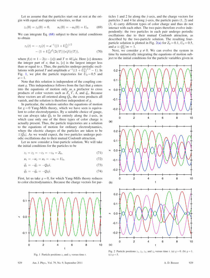
Let us assume that the particles start out at rest at the ori-gin with equal and opposite velocities, so that

z1ð0Þ ¼ z2ð0Þ ¼ 0; u1ð0Þ ¼ �u2ð0Þ ¼ U0: (69)

We can integrate Eq. (68) subject to these initial conditionsto obtain

z1ðtÞ ¼ � z2ðtÞ ¼ a�1ðð1þ U20Þ

1=2

� ð1þ U20 f 2ð2t=TÞÞÞ�ðf ðt=TÞÞ; (70)

where f(x): 1� 2(x� [x]) and T: 4U0/a. Here [x] denotesthe integer part of x; that is, [x] is the largest integer lessthan or equal to x. Thus, the particles undergo periodic oscil-lations with period T and amplitude a�1ðð1þ U2

0Þ1=2 � 1Þ. In

Fig. 1, we plot the particle trajectories for U0¼ 0.5 anda¼ 1.

Note that this solution is independent of the coupling con-stant g. This independence follows from the fact that g entersinto the equations of motion only as a prefactor to crossproducts of color vectors such as ~E, ~V, ~A, and ~qn. Becausethese vectors are all oriented along ~Q0, the cross products allvanish, and the solution is therefore independent of g.

In particular, the solution satisfies the equations of motionfor g¼ 0 Yang-Mills theory, which we have seen is equiva-lent to color electrodynamics. By a suitable choice of gauge,we can always take ~Q0 to lie entirely along the x-axis, inwhich case only one of the three types of color charge isactually present. Thus, the particle trajectories are a solutionto the equations of motion for ordinary electrodynamics,where the electric charges of the particles are taken to be6j~Q0j. As we would expect, the two particles undergo peri-odic oscillations due to their mutual Coulomb attraction.

Let us now consider a four-particle solution. We will takethe initial conditions for the particles to be

z1 ¼ z2 ¼ �z3 ¼ �z4 ¼ Z0; (71)

u1 ¼ �u2 ¼ u3 ¼ �u4 ¼ U0; (72)

~q1 ¼ �~q2 ¼ �Q0x; (73)

~q3 ¼ �~q4 ¼ �Q0y: (74)

First, let us take g¼ 0, for which Yang-Mills theory reducesto color electrodynamics. Because the charge vectors for par-

ticles 1 and 2 lie along the x-axis, and the charge vectors forparticles 3 and 4 lie along y-axis, the particle pairs (1, 2) and(3, 4) carry different types of color charge and thus do notinteract with each other. The two pairs therefore evolve inde-pendently: the two particles in each pair undergo periodicoscillations due to their mutual Coulomb attraction, asdescribed by the two-particle solution. The resulting four-particle solution is plotted in Fig. 2(a) for Z0¼ 0.1, U0¼ 0.5,and a � Q2

0=m ¼ 1.Next, we consider g= 0. We can evolve the system in

time by numerically integrating the equations of motion sub-ject to the initial conditions for the particle variables given in

Fig. 1 Particle positions z1 and z2 versus time t.Fig. 2 Particle positions z1, z2, z3, and z4 versus time t. (a) g¼ 0. (b) g¼ 1.

(c) g¼ 5.

929 Am. J. Phys., Vol. 79, No. 9, September 2011 A. D. Boozer 929

Eqs. (71)–(74).10,11 We also need initial conditions for thefield variables, which we take to be

~Eð0; xÞ ¼ ~Vð0; xÞ ¼ ~Að0; xÞ ¼ 0: (75)

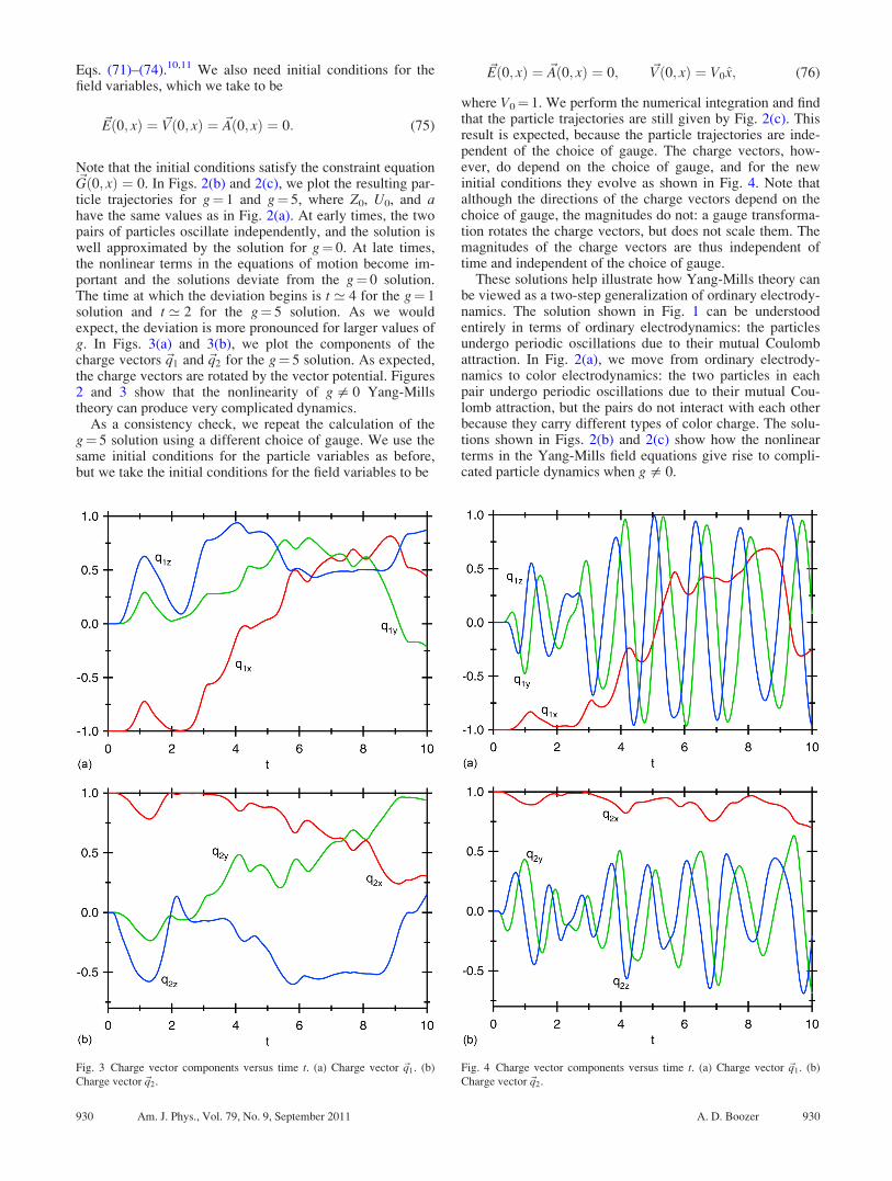
Note that the initial conditions satisfy the constraint equation~Gð0; xÞ ¼ 0. In Figs. 2(b) and 2(c), we plot the resulting par-ticle trajectories for g¼ 1 and g¼ 5, where Z0, U0, and ahave the same values as in Fig. 2(a). At early times, the twopairs of particles oscillate independently, and the solution iswell approximated by the solution for g¼ 0. At late times,the nonlinear terms in the equations of motion become im-portant and the solutions deviate from the g¼ 0 solution.The time at which the deviation begins is t ’ 4 for the g¼ 1solution and t ’ 2 for the g¼ 5 solution. As we wouldexpect, the deviation is more pronounced for larger values ofg. In Figs. 3(a) and 3(b), we plot the components of thecharge vectors ~q1 and ~q2 for the g¼ 5 solution. As expected,the charge vectors are rotated by the vector potential. Figures2 and 3 show that the nonlinearity of g= 0 Yang-Millstheory can produce very complicated dynamics.

As a consistency check, we repeat the calculation of theg¼ 5 solution using a different choice of gauge. We use thesame initial conditions for the particle variables as before,but we take the initial conditions for the field variables to be

~Eð0; xÞ ¼ ~Að0; xÞ ¼ 0; ~Vð0; xÞ ¼ V0x; (76)

where V0¼ 1. We perform the numerical integration and findthat the particle trajectories are still given by Fig. 2(c). Thisresult is expected, because the particle trajectories are inde-pendent of the choice of gauge. The charge vectors, how-ever, do depend on the choice of gauge, and for the newinitial conditions they evolve as shown in Fig. 4. Note thatalthough the directions of the charge vectors depend on thechoice of gauge, the magnitudes do not: a gauge transforma-tion rotates the charge vectors, but does not scale them. Themagnitudes of the charge vectors are thus independent oftime and independent of the choice of gauge.

These solutions help illustrate how Yang-Mills theory canbe viewed as a two-step generalization of ordinary electrody-namics. The solution shown in Fig. 1 can be understoodentirely in terms of ordinary electrodynamics: the particlesundergo periodic oscillations due to their mutual Coulombattraction. In Fig. 2(a), we move from ordinary electrody-namics to color electrodynamics: the two particles in eachpair undergo periodic oscillations due to their mutual Cou-lomb attraction, but the pairs do not interact with each otherbecause they carry different types of color charge. The solu-tions shown in Figs. 2(b) and 2(c) show how the nonlinearterms in the Yang-Mills field equations give rise to compli-cated particle dynamics when g= 0.

Fig. 3 Charge vector components versus time t. (a) Charge vector ~q1. (b)

Charge vector~q2.

Fig. 4 Charge vector components versus time t. (a) Charge vector ~q1. (b)

Charge vector~q2.

930 Am. J. Phys., Vol. 79, No. 9, September 2011 A. D. Boozer 930

VIII. CONCLUSIONS

We have described classical Yang-Mills theory with parti-cle sources and derived the equations of motion for thecoupled particle-field system. As an example, we described indetail the special case of Yang-Mills theory coupled to par-ticles in (1þ 1) dimensions. We presented several examplesolutions and showed that the nonlinearity of the equations ofmotion leads to complicated particle dynamics. The investiga-tion of the particle dynamics in this (1þ 1)-dimensional sys-tem could form the basis of some interesting research projectsfor students.

a)Electronic mail: boozer@unm.edu1An overview of the literature on gauge theory is given in T. P. Cheng and

Ling-Fong Li, “Resource Letter: GI-1 gauge invariance,” Am. J. Phys.

56(7), 586–600 (1988).2The role of gauge theory in describing fundamental interactions is

described in C. Quigg, Gauge Theories of the Strong, Weak, and Electro-magnetic Interactions (Addison-Wesley, New York, 1993).

3The current density given in Eq. (3) is discussed in J. D. Jackson, ClassicalElectrodynamics, 2nd ed. (John Wiley & Sons, New York, 1975), pp. 611–

612.4We generalize to three types of charge, rather than some other number, so

as to obtain the simplest possible version of Yang-Mills theory, which has

gauge group SU(2). More complicated versions of Yang-Mills theory with

larger gauge groups can be obtained by increasing the number of types of

charge. Our definition of “color” is somewhat different from the definition

of “color” in QCD, which has gauge group SU(3).5Because ~h and ~k are infinitesimal, we have neglected terms of second order

in these parameters.6An alternative derivation of the Yang-Mills field strength tensor is given

in Palash B. Pal and K. S. Sateesh, “The field strength and the Lagrangian

of a gauge theory,” Am. J. Phys. 58(8), 789–790 (1990).7Yang-Mills theory was first proposed in C. N. Yang and R. L. Mills,

“Conservation of isotopic spin and isotopic gauge invariance,” Phys. Rev.

96, 191–195 (1954).The coupling of point particles to classical Yang-Mills

fields was first discussed in S. K. Wong, “Field and particle equations for

the classical Yang-Mills field and particles with isotopic spin,” Nuovo

Cimento A 65, 689–694 (1970).8Electrodynamics in (1þ 1) dimensions is discussed in many places. See,

for example, I. Bialynicki-Birula, “Classical electrodynamics in two

dimensions: Exact solution,” Phys. Rev. D 3, 864–866 (1971) and the ap-

pendix of Ref. 10.9We have replaced 4p, the appropriate solid angle factor for (3þ 1) dimen-

sions, by 2, the appropriate solid angle factor for (1þ 1) dimensions. The

appropriate solid angle factor for (dþ 1) dimensions is given by the area

of a d-dimensional sphere, which is 2pd/2/C(d/2).10The methods used to perform the numerical integration are described in A.

D. Boozer, “Simulating a toy model of electrodynamics in (1þ 1)

dimensions,” Am. J. Phys. 77(3), 262–269 (2009).11The program used to perform the numerical integration is available upon

request.

931 Am. J. Phys., Vol. 79, No. 9, September 2011 A. D. Boozer 931