Classical Simulation of Quantum Supremacy Circuits

Cupjin Huang,1 Fang Zhang,2 Michael Newman,3 Junjie Cai,4

Xun Gao,1 Zhengxiong Tian,5 Junyin Wu,4 Haihong Xu,5 Huanjun Yu,5

Bo Yuan,6 Mario Szegedy,1 Yaoyun Shi1, Jianxin Chen1

1Alibaba Quantum Laboratory,Alibaba Group USA, Bellevue, WA 98004, USA

2Department of Electrical Engineering and Computer Science,University of Michigan, Ann Arbor, MI 48109, USA

3Departments of Physics and Electrical and Computer Engineering,Duke University, Durham, NC 27708, USA

4Alibaba Cloud Intelligence,Alibaba Group USA, Bellevue, WA 98004, USA

5Alibaba Cloud Intelligence,Alibaba Group, Hangzhou, Zhejiang 310000, China

6Alibaba Infrastructure Service,Alibaba Group, Hangzhou, Zhejiang 310000, China

AbstractIt is believed that random quantum circuits are difficult to simulate classically. These

have been used to demonstrate quantum supremacy: the execution of a computational taskon a quantum computer that is infeasible for any classical computer. The task underly-ing the assertion of quantum supremacy by Arute et al. (Nature, 574, 505–510 (2019))was initially estimated to require Summit, the world’s most powerful supercomputer to-day, approximately 10,000 years. The same task was performed on the Sycamore quantumprocessor in only 200 seconds.

In this work, we present a tensor network-based classical simulation algorithm. Usinga Summit-comparable cluster, we estimate that our simulator can perform this task in lessthan 20 days. On moderately-sized instances, we reduce the runtime from years to minutes,running several times faster than Sycamore itself. These estimates are based on explicitsimulations of parallel subtasks, and leave no room for hidden costs. The simulator’s keyingredient is identifying and optimizing the “stem” of the computation: a sequence of pair-wise tensor contractions that dominates the computational cost. This orders-of-magnitude

1

arX

iv:2

005.

0678

7v1

[qu

ant-

ph]

14

May

202

0

reduction in classical simulation time, together with proposals for further significant im-provements, indicates that achieving quantum supremacy may require a period of continu-ing quantum hardware developments without an unequivocal first demonstration.

1 IntroductionQuantum computers offer the promise of exponential speedups over classical computers. Con-sequently, as quantum technologies grow, there will be an inevitable crossing point after whichnascent quantum processors will overtake behemoth classical computing systems on specializedtasks. The term “quantum supremacy” was coined to describe this watershed moment [1].

Sampling from random quantum circuits is ideal for this purpose. Although it may nothave practical value, it is straightforward to perform on a quantum processor: execute a randomsequence of quantum gates and then output the measurement result of each qubit. The centralchallenge is in building a quantum processor of sufficient size and accuracy so that samplingthese outcomes becomes infeasible for a classical computer. The hardness of such tasks hasbeen well-studied [2, 3, 4, 5, 6], and is more broadly founded on the expectation that classicallysimulating general quantum circuits takes a time that grows exponentially with the circuit size.

In [7], the authors sample from a family of random quantum circuits run on the 53-qubitSycamore device at increasing depth, measured in terms of “cycles”. As quantum gates arenoisy, the quantum device samples from a noisy version of the ideal distribution; however, witha sufficient number of samples, the signal can be reliably recovered. Sycamore’s performanceis a remarkable engineering achievement, and quantum supremacy has been widely discussed.However, it is based on the authors’ own best classical runtime estimates. As they themselvespoint out, simulators will continue to improve, and so these estimates may fall short of the truepotential of classical computers [7].

1.1 ResultsIn this work, we push back against the classical simulation barrier. We introduce and bench-mark a powerful new tensor network-based simulator that dramatically reduces the computa-tional cost of sampling from random quantum circuits. On 53-qubit random quantum circuitswith 20 cycles, we estimate that it can sample a near-perfect output in minutes. This reducesthe runtime of collecting one million samples from a 20-cycle circuit adjusted for a 0.2% fi-delity from 10, 000 years to less than 20 days. On 14-cycle circuits, we reduce the runtimeof collecting three million samples with 1% fidelity from 1.1 years to 264 seconds, twice asfast as the total execution time on Sycamore [7, 8]. These estimates were obtained by divid-ing the embarrassingly parallelizable problem into nearly-identical subtasks that run in parallel.These subtasks were then explicitly benchmarked on Summit-comparable nodes within AlibabaCloud, yielding a precise estimate while avoiding resource-intensive full-scale simulation.

2

1.2 Technical contributions and comparisonsIn addition to developing and conglomerating a number of technical optimizations, we achievethese runtimes by introducing a powerful new method for simulating quantum circuits: stemoptimization. The key insight is that the random circuits in [7], which are subject to the 2Dnearest-neighbor constraints of the device, are highly regular tensor networks. This regularitymanifests at the level of tensor network contraction as a single stem: a path of contractions thatdominates the overall cost of the computation. By identifying and optimizing this stem, weare able to increase the efficiency of our simulator to 1, 000× the efficiency of the state-of-the-art simulator introduced in [9], and to approximately 200, 000× the efficiency of the originalestimate in [7].

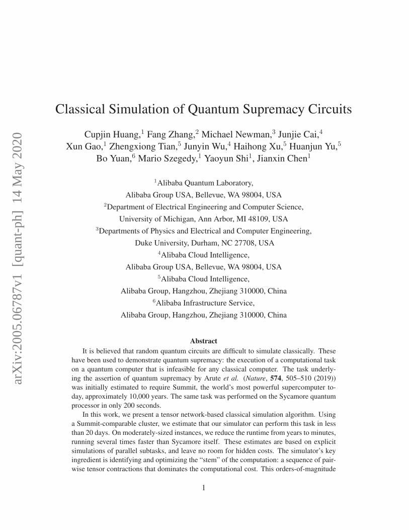
Figure 1: Tensor network contraction of a quantum circuit from the random circuit family [7],visualized as a binary contraction tree. Each node in the tree represents a step in the contraction.Larger, darker nodes indicate more expensive steps. The central stem dominates the overallcontraction cost.

Several challenges have been levied against quantum supremacy. The most relevant to thiswork is not an explicit simulator, but rather a proposal by Pednault et al. [10] to leverage theimmense secondary storage on Summit to perform full state-vector updates [11, 12]. It estimatesthat the quantum supremacy task at 20 cycles can be accomplished in 2.5 days. There are twomain drawbacks to this work. First, although this simulation strategy scales linearly in depth,it runs into a hard memory limit with even a small increase in the number of qubits. Second,the estimate is based on optimistic assumptions that are difficult to judge without real device-level tests. Even if we make only a small subset of analogous assumptions, we estimate thatrunning qFlex [8] on tasks generated by our algorithm would already reduce the runtime to lessthan two days. This uses its out-of-core tensor contraction capabilities while assuming that theFLOPS efficiency reported in [7] is preserved; see Section A.4 of the supplementary materialfor more details. We reemphasize that these are proposals; it is difficult to judge their feasibilityor accuracy without an explicit simulator tested on a Summit-comparable platform, and maylead to orders-of-magnitude differences.

3

Our simulator produces samples extremely quickly, on the order of minutes for each, sothat the overall task remains fast when adjusted for the low fidelity of the quantum computer.At its core, our tensor network-based algorithm dynamically decomposes the computationaltask into many smaller subtasks that can be executed in parallel on a cluster. This allows usto trade space for time, avoiding the hard memory limits of full state-vector update simulators[12, 10]. Consequently, our simulator will not be overwhelmed by adding a small numberof qubits [13]. Furthermore, we can accurately estimate the total runtime of our approachusing explicit simulations. All of the subtasks have the same tensor network structure, andso their individual runtimes are nearly identical. In addition, each is completed without anycommunication between nodes. There is indeed some communication when distributing thesubtasks and collecting their results, but it is negligibly small. This was verified by a large-scalecomputational experiment conducted using 127,512 cores of the Elastic Computing Services atAlibaba Cloud; see Section A.4 in the supplementary material.

As tensor networks are ubiquitous in quantum information science, with applications includ-ing benchmarking quantum devices [7, 14], probing quantum many-body systems [15, 16, 17,18], and decoding quantum error-correcting codes [19, 20, 21], our simulator represents a pow-erful new tool to aid in the development of quantum technologies. Technical reports [13, 22, 23]detail the use of earlier iterations of Alibaba Cloud Quantum Development Platform (AC-QDP)for algorithm design and surface code simulation.

2 Sycamore Random Quantum CircuitsIn this work, we focus on the random quantum circuits executed on the 53-qubit Sycamorequantum chip [7]. Every random circuit is composed of m cycles, each consisting of a single-qubit gate layer and a two-qubit gate layer, and concludes with an additional single-qubit gatelayer preceding measurement in the computational basis. In the first single-qubit gate layer,single-qubit gates are chosen for each individual qubit independently and uniformly at randomfrom {

√X,√Y ,√W}, where

√X =

1√2

[1 −i−i 1

],√Y =

1√2

[1 −11 1

],√W =

1√2

[1 −

√i√

−i 1

].

In each successive single-qubit gate layer, single-qubit gates are chosen for each individual qubituniformly at random from the subset of {

√X,√Y ,√W} that excludes the single-qubit gate

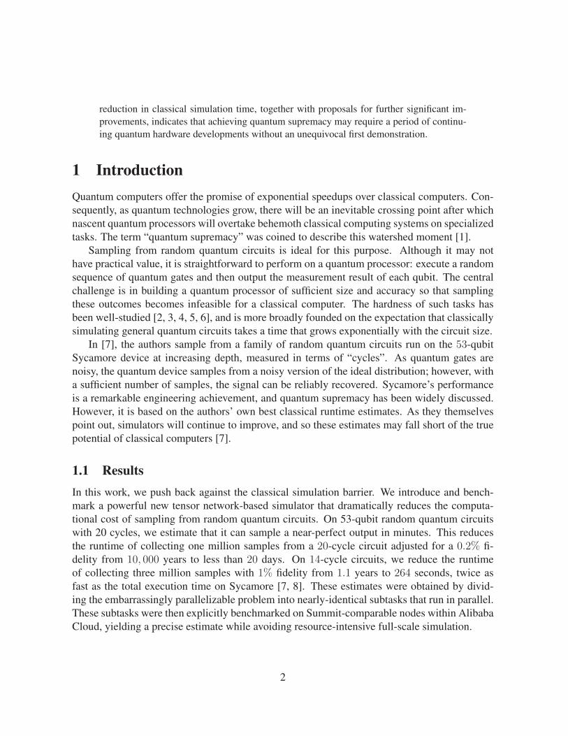
applied in the previous cycle. In two-qubit gate layers, two-qubit gates are applied accordingto a specified pairing of qubits in different cycles. There are four different patterns of pairings,depicted in Figure 2, and we repeat the 8-cycle pattern A, B, C, D, C, D, A, B. Two-qubit gates

4

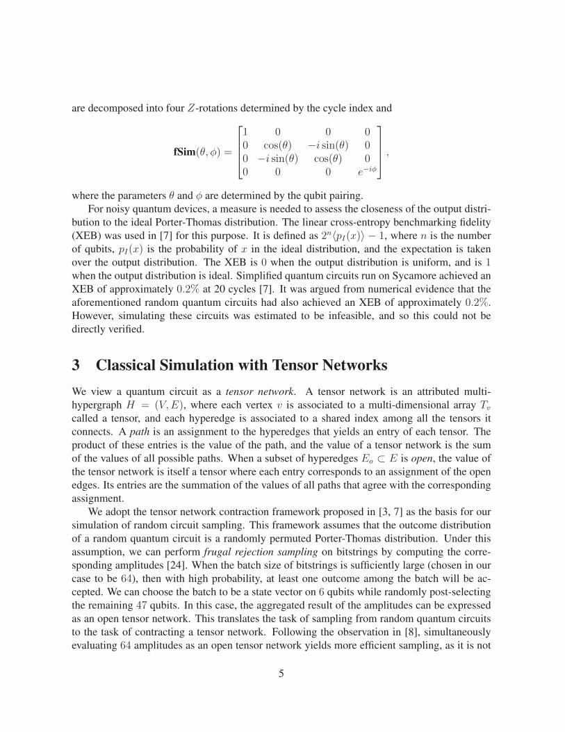
are decomposed into four Z-rotations determined by the cycle index and

fSim(θ, φ) =

1 0 0 00 cos(θ) −i sin(θ) 00 −i sin(θ) cos(θ) 00 0 0 e−iφ

,where the parameters θ and φ are determined by the qubit pairing.

For noisy quantum devices, a measure is needed to assess the closeness of the output distri-bution to the ideal Porter-Thomas distribution. The linear cross-entropy benchmarking fidelity(XEB) was used in [7] for this purpose. It is defined as 2n〈pI(x)〉 − 1, where n is the numberof qubits, pI(x) is the probability of x in the ideal distribution, and the expectation is takenover the output distribution. The XEB is 0 when the output distribution is uniform, and is 1when the output distribution is ideal. Simplified quantum circuits run on Sycamore achieved anXEB of approximately 0.2% at 20 cycles [7]. It was argued from numerical evidence that theaforementioned random quantum circuits had also achieved an XEB of approximately 0.2%.However, simulating these circuits was estimated to be infeasible, and so this could not bedirectly verified.

3 Classical Simulation with Tensor NetworksWe view a quantum circuit as a tensor network. A tensor network is an attributed multi-hypergraph H = (V,E), where each vertex v is associated to a multi-dimensional array Tvcalled a tensor, and each hyperedge is associated to a shared index among all the tensors itconnects. A path is an assignment to the hyperedges that yields an entry of each tensor. Theproduct of these entries is the value of the path, and the value of a tensor network is the sumof the values of all possible paths. When a subset of hyperedges Eo ⊂ E is open, the value ofthe tensor network is itself a tensor where each entry corresponds to an assignment of the openedges. Its entries are the summation of the values of all paths that agree with the correspondingassignment.

We adopt the tensor network contraction framework proposed in [3, 7] as the basis for oursimulation of random circuit sampling. This framework assumes that the outcome distributionof a random quantum circuit is a randomly permuted Porter-Thomas distribution. Under thisassumption, we can perform frugal rejection sampling on bitstrings by computing the corre-sponding amplitudes [24]. When the batch size of bitstrings is sufficiently large (chosen in ourcase to be 64), then with high probability, at least one outcome among the batch will be ac-cepted. We can choose the batch to be a state vector on 6 qubits while randomly post-selectingthe remaining 47 qubits. In this case, the aggregated result of the amplitudes can be expressedas an open tensor network. This translates the task of sampling from random quantum circuitsto the task of contracting a tensor network. Following the observation in [8], simultaneouslyevaluating 64 amplitudes as an open tensor network yields more efficient sampling, as it is not

5

0

1

2

3

4

5

6

7

8

9

10

11

12

13

14

15

16

17

18

19

20

21

22

23

24

25

26

27

28

29

30

31

32

33

34

35

36

37

38

39

40

41

42

43

44

45

46

47

48

49

50

5152

(a)

|0〉

A B C D C D A B

|0〉

|0〉

|0〉

|0〉(b)

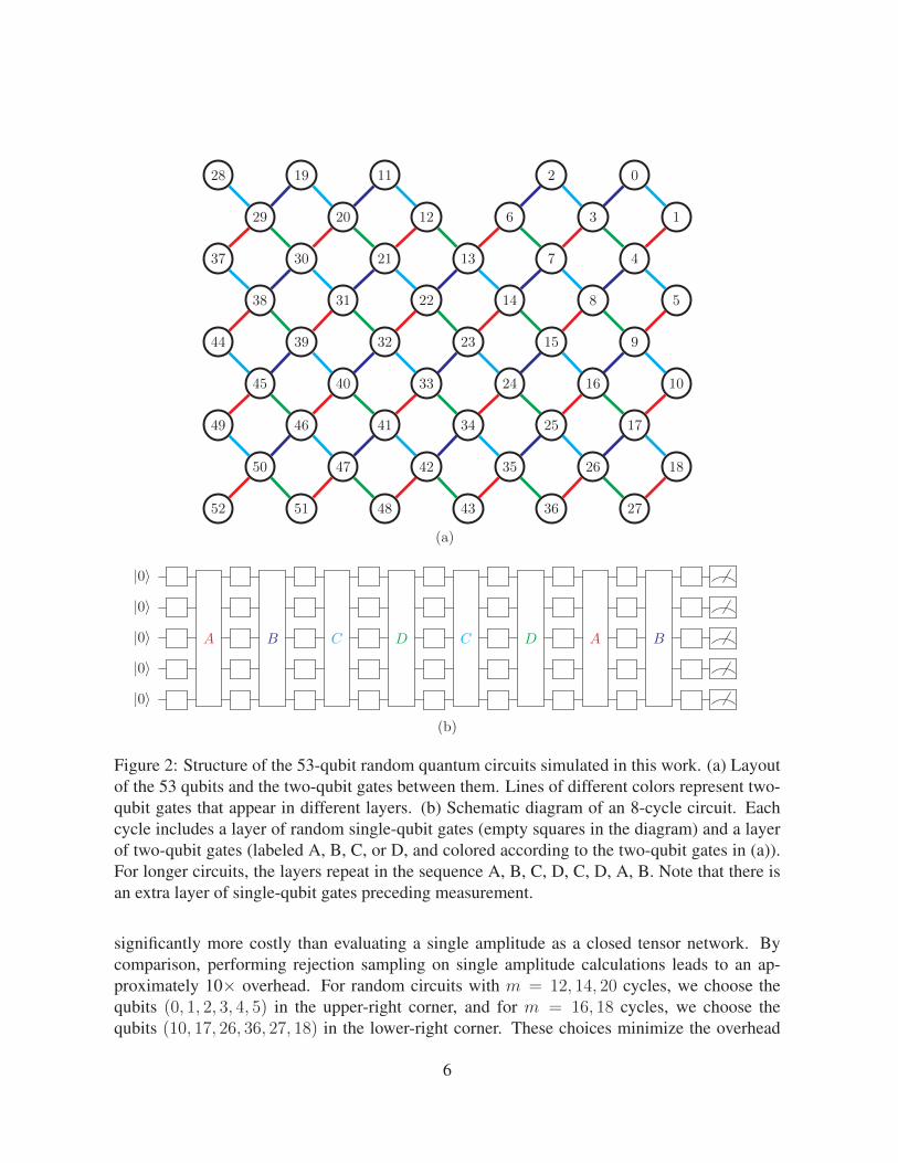
Figure 2: Structure of the 53-qubit random quantum circuits simulated in this work. (a) Layoutof the 53 qubits and the two-qubit gates between them. Lines of different colors represent two-qubit gates that appear in different layers. (b) Schematic diagram of an 8-cycle circuit. Eachcycle includes a layer of random single-qubit gates (empty squares in the diagram) and a layerof two-qubit gates (labeled A, B, C, or D, and colored according to the two-qubit gates in (a)).For longer circuits, the layers repeat in the sequence A, B, C, D, C, D, A, B. Note that there isan extra layer of single-qubit gates preceding measurement.

significantly more costly than evaluating a single amplitude as a closed tensor network. Bycomparison, performing rejection sampling on single amplitude calculations leads to an ap-proximately 10× overhead. For random circuits with m = 12, 14, 20 cycles, we choose thequbits (0, 1, 2, 3, 4, 5) in the upper-right corner, and for m = 16, 18 cycles, we choose thequbits (10, 17, 26, 36, 27, 18) in the lower-right corner. These choices minimize the overhead

6

introduced by simultaneously evaluating each batch of amplitudes.There are two approaches for performing tensor network contraction, namely the Feynman

method and the Schrodinger method.

The Feynman method The Feynman method computes the value of each path separately, andsums over all possible paths. This takes a polynomial amount of space to store the currentresult and path, but takes a number of steps that scales exponentially with the number ofhyperedges. Such high time complexity renders this approach infeasible for even smalltensor networks consisting of only 50 to 100 hyperedges.

The Schrodinger method The Schrodinger method performs sequential pairwise contractions.At each step, two vertices in the hypergraph are chosen. The corresponding tensors arecontracted according to their shared indices, and the two-vertex subgraph is replaced bya single vertex representing the newly formed tensor. This process is repeated until onlyone vertex is left. Up to transposition, this tensor is the final result and does not dependon the ordering of vertices contracted at each step. Although we can find a contractionorder that nearly minimizes the total time complexity [25], the space complexity scalesexponentially with the contraction width of the hypergraph [26]. This usually exceeds theaccessible memory of a single computational device when simulating intermediate-sizequantum circuits.

We use a hybrid method to find an acceptable tradeoff between space and time. We firstchoose a small subset of indices. For each assignment of these indices, the computationalsubtask is itself a tensor network contraction, where each sub-tensor network corresponds to thefull tensor network with the fixed hyperedges removed. Contracting these sub-tensor networksis perfectly parallellizable, and the space complexity of each subtask is significantly smallerthan that of the full task. The hybrid method allows one to trade between space and time, butit requires cleverly choosing an efficient contraction scheme, which includes a good subset ofindices as well as an efficient contraction sequence for each subtask.

Determining an optimal contraction scheme is itself a computationally hard problem. How-ever, extensive work has been devoted to finding good contraction schemes, including the intro-duction of hyperedges [3], dynamic edge-slicing [27], open tensor network contraction [8, 23],and hypergraph-decomposition-based contraction [9]. Our simulator is a culmination of ad-vances, beginning with [27] and extended in [13, 22, 23]. By incorporating a series of newlydeveloped algorithmic ideas and polishing existing ones, we are able to find a good contractionscheme in a reasonable amount of time.

4 Stem OptimizationThe main insight of our work is not how to optimize the contraction sequence but where tooptimize it. We observe a generic structure appearing in this family of random quantum cir-cuits: a computationally-intensive stem that emerges in a typical contraction tree associated to

7

a circuit’s tensor network. A contraction tree is a binary tree whose leaf nodes represent initialtensors and whose internal nodes represent intermediate tensors formed from the pairwise con-traction of their children. We can associate to each internal node the time and space complexityof its corresponding pairwise contraction step.

We observe that a typical contraction tree consists of a single path of expensive nodes whichwe call the stem, along with small clusters of inexpensive nodes which we call branches, as inFigure 1. Almost all of the computation happens along the stem, where a single big tensorabsorbs small tensors representing the results from each branch sequentially. Moreover, thelength of the stem is usually small compared to the total number of nodes in the contractiontree.

By focusing our attention on the stem, we are able to achieve tremendous speedups in thesimulation of random quantum circuits. The techniques we use to realize these speedups, whichwe call stem optimization, include the following (see Section A.2 of the supplementary materialfor more details).

Hypergraph partitioning Introduced in [9], hypergraph partitioning can find a good contrac-tion tree in a top-down manner. It divides the vertices of a hypergraph into several com-ponents so that the size of each component is neither too small nor too big, while min-imizing the number of interconnecting hyperedges. It first contracts each component toa single vertex, and then contracts the remaining nodes together. The sub-contractiontree associated to each component can be computed recursively while the top-layer of thecontraction tree that merges the components can be found by brute force. This brute forcesearch will have low cost because of the small number of interconnecting edges.

Unlike [9], we first multi-partition at the top level to find one or two major componentscontaining the stem, and then recursively bipartition the stem components to strip off thebranches one by one. A single run of recursive hypergraph partitioning yields a candidatecontraction tree. Using the contraction cost of the tree as our objective function, weoptimize the parameters of this process (such as the imbalance parameters for each layer)over multiple runs of the recursive partitioning.

Local optimization After constructing a good initial contraction tree, we perform local opti-mizations to further reduce the contraction cost. A connected subgraph of the contractiontree is itself a contraction tree, and its internal connections can be rearranged withoutaffecting other parts of the tree. This allows us to arbitrarily select small connected sub-graphs of the contraction tree where brute-force optimization is feasible, and optimizeover the chosen subgraphs. We focus on optimizing subpaths of the stem, as this is wheremost of the computation occurs. Figure 8 in the supplementary material illustrates localoptimization by switching two branches.

Dynamic slicing To simultaneously determine a subset of indices to enumerate as well as agood contraction tree for each sub-tensor network, we first find a good contraction treefor the full task and then choose indices based on that tree. In a contraction tree, all nodes

8

with a shared index form a subtree, and enumerating over that index in the tensor networkremoves it from the resulting contraction tree. Dynamic slicing was first introduced by usin [27], and subsequently adopted in several other simulators [8, 13, 23, 9, 28].

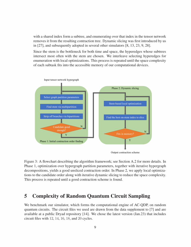
Since the stem is the bottleneck for both time and space, the hyperedges whose subtreesintersect most often with the stem are chosen. We interleave selecting hyperedges forenumeration with local optimizations. This process is repeated until the space complexityof each subtask fits into the accessible memory of our computational devices.

Stem-based local optimization

Find the best on-stem index to slice

Fits in memory?

Output contraction scheme

Phase 2: Dynamic slicing

Y

N

Input tensor network hypergraph

Find stem via multipartition

Strip off branches via bipartitions

Candidate good enough?

Phase 1: Initial contraction order finding

Select graph partition parameters

Y

N

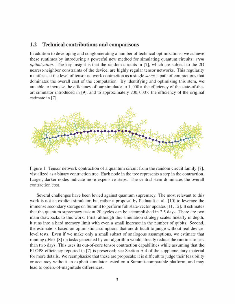
Figure 3: A flowchart describing the algorithm framework; see Section A.2 for more details. InPhase 1, optimization over hypergraph partition parameters, together with iterative hypergraphdecompositions, yields a good unsliced contraction order. In Phase 2, we apply local optimiza-tions to the candidate order along with iterative dynamic slicing to reduce the space complexity.This process is repeated until a good contraction scheme is found.

5 Complexity of Random Quantum Circuit SamplingWe benchmark our simulator, which forms the computational engine of AC-QDP, on randomquantum circuits. The circuit files we used are drawn from the data supplement to [7] and areavailable at a public Dryad repository [14]. We chose the latest version (Jan.23) that includescircuit files with 12, 14, 16, 18, and 20 cycles.

9

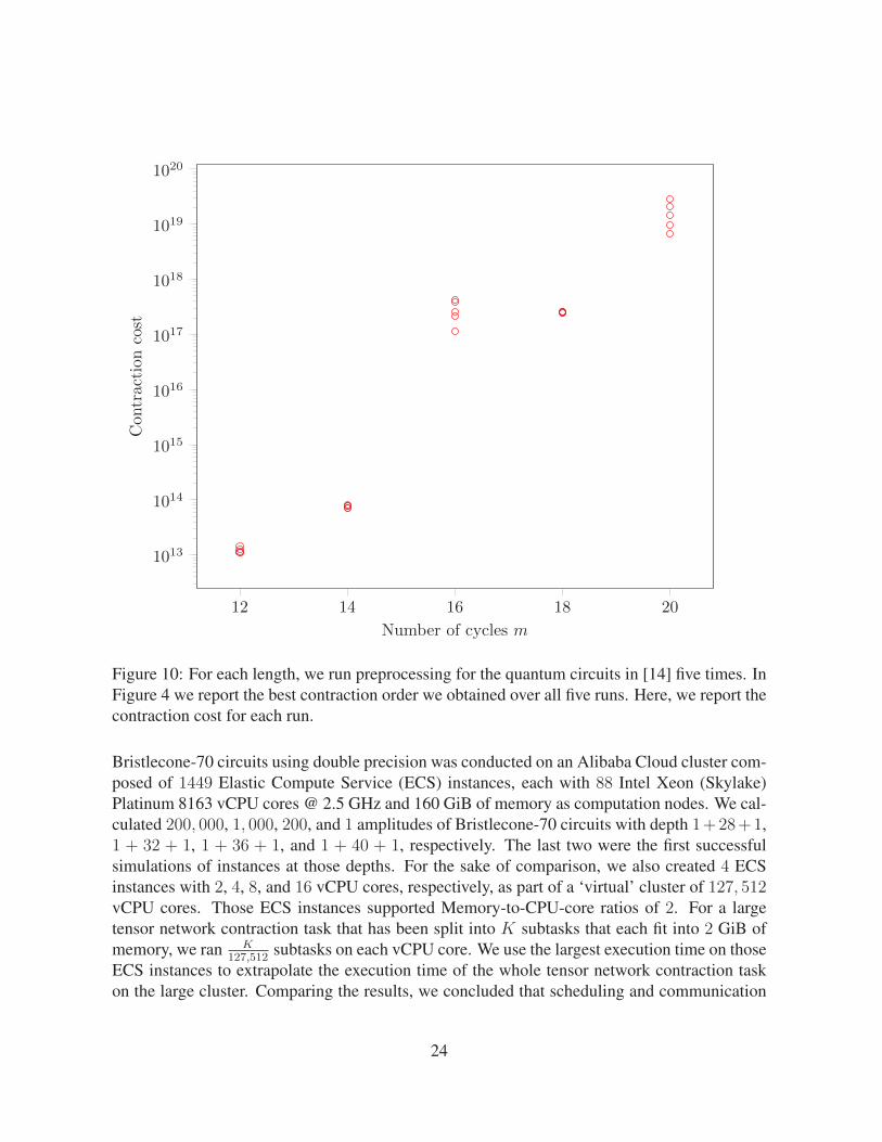
In the preprocessing step for generating a contraction order, we allow for 50 iterations ofCMA-ES for parameter optimization and choose the number of local optimization iterationsbefore, between, and after slicing to be 20, 20, and 50, respectively. The generated contractionorder is then distributed to the computational nodes. We run each circuit 5 times and choose thebest contraction order. Figure 10 in the supplementary material shows the contraction cost foreach run. Detailed information about our cluster architecture can also be found in Section A.4.

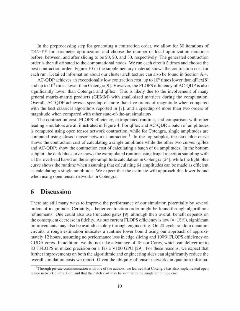
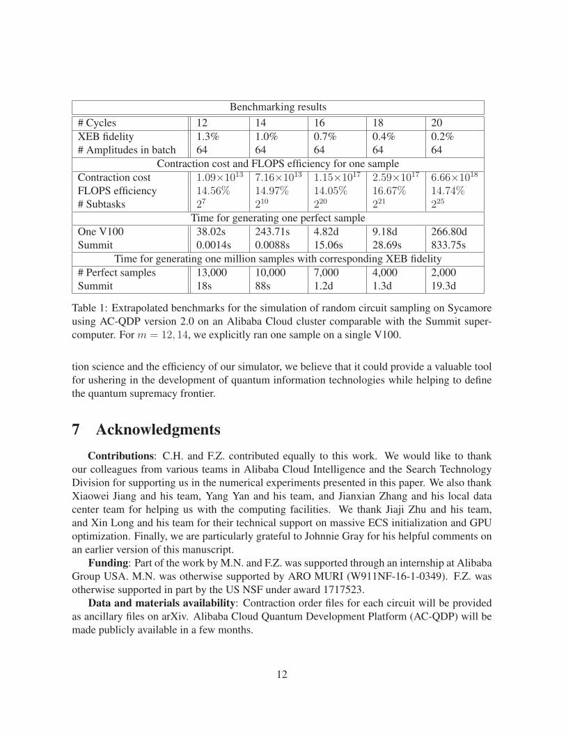
AC-QDP achieves an exceptionally low contraction cost, up to 106 times lower than qFlex[8]and up to 103 times lower than Cotengra[9]. However, the FLOPS efficiency of AC-QDP is alsosignificantly lower than Cotengra and qFlex. This is likely due to the involvement of manygeneral matrix-matrix products (GEMM) with small-sized matrices during the computation.Overall, AC-QDP achieves a speedup of more than five orders of magnitude when comparedwith the best classical algorithms reported in [7], and a speedup of more than two orders ofmagnitude when compared with other state-of-the-art simulators.

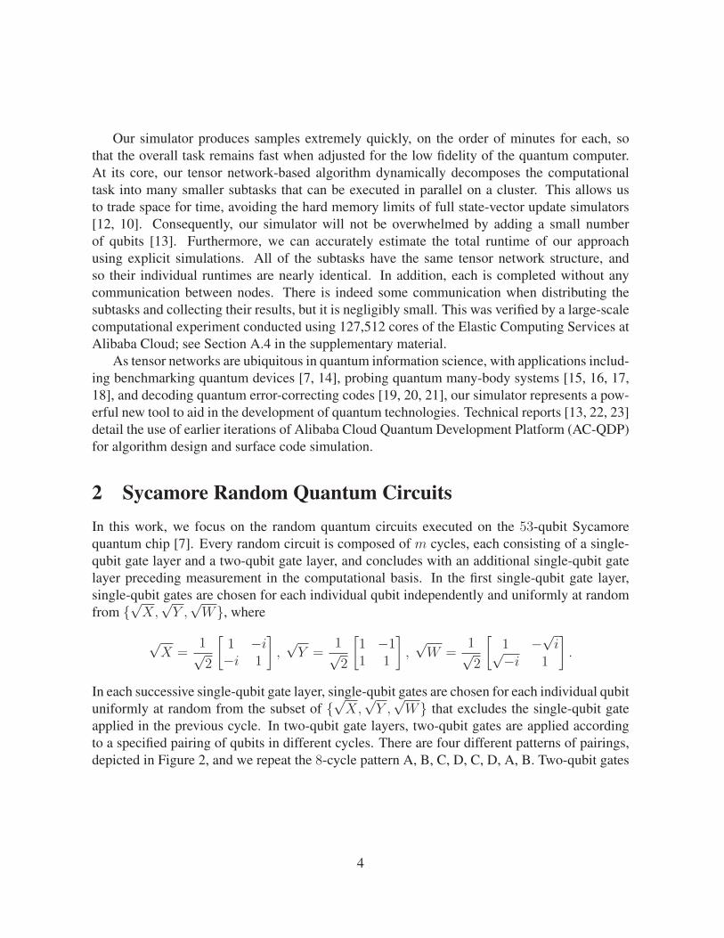
The contraction cost, FLOPS efficiency, extrapolated runtime, and comparison with otherleading simulators are all illustrated in Figure 4. For qFlex and AC-QDP, a batch of amplitudesis computed using open tensor network contraction, while for Cotengra, single amplitudes arecomputed using closed tensor network contraction.1 In the top subplot, the dark blue curveshows the contraction cost of calculating a single amplitude while the other two curves (qFlexand AC-QDP) show the contraction cost of calculating a batch of 64 amplitudes. In the bottomsubplot, the dark blue curve shows the extrapolated runtime using frugal rejection sampling witha 10× overhead based on the single-amplitude calculation in Cotengra [24], while the light bluecurve shows the runtime when assuming that calculating 64 amplitudes can be made as efficientas calculating a single amplitude. We expect that the estimate will approach this lower boundwhen using open tensor networks in Cotengra.

6 DiscussionThere are still many ways to improve the performance of our simulator, potentially by severalorders of magnitude. Certainly, a better contraction order might be found through algorithmicrefinements. One could also use truncated gates [9], although their overall benefit depends onthe consequent decrease in fidelity. As our current FLOPS efficiency is low (≈ 15%), significantimprovements may also be available solely through engineering. On 20-cycle random quantumcircuits, a rough estimation indicates a runtime lower bound using our approach of approxi-mately 12 hours, assuming no performance loss in edge slicing and 100% FLOPS efficiency onCUDA cores. In addition, we did not take advantage of Tensor Cores, which can deliver up to83 TFLOPS in mixed precision on a Tesla V100 GPU [29]. For these reasons, we expect thatfurther improvements on both the algorithmic and engineering sides can significantly reduce theoverall simulation costs we report. Given the ubiquity of tensor networks in quantum informa-

1Through private communication with one of the authors, we learned that Cotengra has also implemented opentensor network contraction, and that the batch cost may be similar to the single amplitude cost.

10

1013

1015

1017

1019

1021C

ontr

acti

onco

stqFlex (batch)

Cotengra (amplitude)

AC-QDP (batch)

20%

40%

60%

80%

100%

FL

OP

Seffi

cien

cy

qFlex (batch)

Cotengra (amplitude)

AC-QDP (batch)

12(1.3%)

14(1.0%)

16(0.7%)

18(0.4%)

20(0.2%)

101

104

107

1010

Number of cycles m and corresponding XEB fidelities

Extr

apola

ted

runti

me

(s)

qFlex

Supremacy simulations (7)

Cotengra (amplitude)

Cotengra LB

AC-QDP

1 millenium

1 year

1 day

Sycamore

Figure 4: Classical simulation cost of sampling from m-cycle random circuits with low XEBfidelities. Numerical data is reported in Table 1.

11

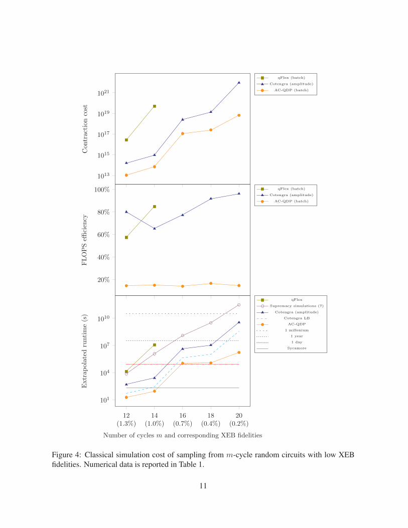
Benchmarking results# Cycles 12 14 16 18 20XEB fidelity 1.3% 1.0% 0.7% 0.4% 0.2%# Amplitudes in batch 64 64 64 64 64

Contraction cost and FLOPS efficiency for one sampleContraction cost 1.09×1013 7.16×1013 1.15×1017 2.59×1017 6.66×1018FLOPS efficiency 14.56% 14.97% 14.05% 16.67% 14.74%# Subtasks 27 210 220 221 225

Time for generating one perfect sampleOne V100 38.02s 243.71s 4.82d 9.18d 266.80dSummit 0.0014s 0.0088s 15.06s 28.69s 833.75s

Time for generating one million samples with corresponding XEB fidelity# Perfect samples 13,000 10,000 7,000 4,000 2,000Summit 18s 88s 1.2d 1.3d 19.3d

Table 1: Extrapolated benchmarks for the simulation of random circuit sampling on Sycamoreusing AC-QDP version 2.0 on an Alibaba Cloud cluster comparable with the Summit super-computer. For m = 12, 14, we explicitly ran one sample on a single V100.

tion science and the efficiency of our simulator, we believe that it could provide a valuable toolfor ushering in the development of quantum information technologies while helping to definethe quantum supremacy frontier.

7 AcknowledgmentsContributions: C.H. and F.Z. contributed equally to this work. We would like to thank

our colleagues from various teams in Alibaba Cloud Intelligence and the Search TechnologyDivision for supporting us in the numerical experiments presented in this paper. We also thankXiaowei Jiang and his team, Yang Yan and his team, and Jianxian Zhang and his local datacenter team for helping us with the computing facilities. We thank Jiaji Zhu and his team,and Xin Long and his team for their technical support on massive ECS initialization and GPUoptimization. Finally, we are particularly grateful to Johnnie Gray for his helpful comments onan earlier version of this manuscript.

Funding: Part of the work by M.N. and F.Z. was supported through an internship at AlibabaGroup USA. M.N. was otherwise supported by ARO MURI (W911NF-16-1-0349). F.Z. wasotherwise supported in part by the US NSF under award 1717523.

Data and materials availability: Contraction order files for each circuit will be providedas ancillary files on arXiv. Alibaba Cloud Quantum Development Platform (AC-QDP) will bemade publicly available in a few months.

12

References[1] John Preskill. Quantum computing and the entanglement frontier. arXiv preprint

arXiv:1203.5813, 2012.

[2] Scott Aaronson and Lijie Chen. Complexity-theoretic foundations of quantum supremacyexperiments. In 32nd Computational Complexity Conference (CCC 2017). SchlossDagstuhl-Leibniz-Zentrum fuer Informatik, 2017.

[3] Sergio Boixo, Sergei V Isakov, Vadim N Smelyanskiy, Ryan Babbush, Nan Ding, ZhangJiang, Michael J Bremner, John M Martinis, and Hartmut Neven. Characterizing quantumsupremacy in near-term devices. Nature Physics, 14(6):595–600, 2018.

[4] Adam Bouland, Bill Fefferman, Chinmay Nirkhe, and Umesh Vazirani. On the complexityand verification of quantum random circuit sampling. Nature Physics, 15(2):159–163,2019.

[5] Scott Aaronson and Sam Gunn. On the classical hardness of spoofing linear cross-entropybenchmarking. arXiv preprint arXiv:1910.12085, 2019.

[6] Alexander Zlokapa, Sergio Boixo, and Daniel Lidar. Boundaries of quantum supremacyvia random circuit sampling. arXiv preprint arXiv:2005.02464, 2020.

[7] Frank Arute, Kunal Arya, Ryan Babbush, Dave Bacon, Joseph C Bardin, Rami Barends,Rupak Biswas, Sergio Boixo, Fernando GSL Brandao, David A Buell, et al. Quantumsupremacy using a programmable superconducting processor. Nature, 574(7779):505–510, 2019.

[8] Benjamin Villalonga, Sergio Boixo, Bron Nelson, Christopher Henze, Eleanor Rieffel,Rupak Biswas, and Salvatore Mandra. A flexible high-performance simulator for veri-fying and benchmarking quantum circuits implemented on real hardware. NPJ QuantumInformation, 5:1–16, 2019.

[9] Johnnie Gray and Stefanos Kourtis. Hyper-optimized tensor network contraction. arXivpreprint arXiv:2002.01935, 2020.

[10] Edwin Pednault, John A Gunnels, Giacomo Nannicini, Lior Horesh, and Robert Wisnieff.Leveraging secondary storage to simulate deep 54-qubit sycamore circuits. arXiv preprintarXiv:1910.09534, 2019.

[11] Thomas Haner and Damian S Steiger. 0.5 petabyte simulation of a 45-qubit quantumcircuit. In Proceedings of the International Conference for High Performance Computing,Networking, Storage and Analysis, pages 1–10, 2017.

13

[12] Edwin Pednault, John A Gunnels, Giacomo Nannicini, Lior Horesh, Thomas Magerlein,Edgar Solomonik, Erik W Draeger, Eric T Holland, and Robert Wisnieff. Breaking the49-qubit barrier in the simulation of quantum circuits. arXiv preprint arXiv:1710.05867,2017.

[13] Fang Zhang, Cupjin Huang, Michael Newman, Junjie Cai, Huanjun Yu, Zhengxiong Tian,Bo Yuan, Haihong Xu, Junyin Wu, Xun Gao, Jianxin Chen, Mario Szegedy, and YaoyunShi. Alibaba cloud quantum development platform: Large-scale classical simulation ofquantum circuits. arXiv preprint arXiv:1907.11217, 2019.

[14] Frank Arute, Kunal Arya, Ryan Babbush, Dave Bacon, Joseph C Bardin, Rami Barends,Rupak Biswas, Sergio Boixo, Fernando GSL Brandao, David A Buell, et al. Quan-tum supremacy using a programmable superconducting processor. arXiv preprintarXiv:1910.11333, 2019. Data retrieved from datadryad.org, https://datadryad.org/stash/dataset/doi:10.5061/dryad.k6t1rj8.

[15] Steven R White. Density matrix formulation for quantum renormalization groups. Physi-cal Review Letters, 69(19):2863, 1992.

[16] Guifre Vidal. Efficient classical simulation of slightly entangled quantum computations.Physical Review Letters, 91(14):147902, 2003.

[17] Guifre Vidal. Classical simulation of infinite-size quantum lattice systems in one spatialdimension. Physical Review Letters, 98(7):070201, 2007.

[18] Ulrich Schollwock. The density-matrix renormalization group. Reviews of ModernPhysics, 77(1):259, 2005.

[19] Sergey Bravyi, Martin Suchara, and Alexander Vargo. Efficient algorithms for maximumlikelihood decoding in the surface code. Physical Review A, 90(3):032326, 2014.

[20] Andrew J Ferris and David Poulin. Tensor networks and quantum error correction. Phys-ical Review Letters, 113(3):030501, 2014.

[21] Christopher T Chubb and Steven T Flammia. Statistical mechanical models for quantumcodes with correlated noise. arXiv preprint arXiv:1809.10704, 2018.

[22] Cupjin Huang, Mario Szegedy, Fang Zhang, Xun Gao, Jianxin Chen, and Yaoyun Shi.Alibaba cloud quantum development platform: Applications to quantum algorithm design.arXiv preprint arXiv:1909.02559, 2019.

[23] Cupjin Huang, Xiaotong Ni, Fang Zhang, Michael Newman, Dawei Ding, Xun Gao,Tenghui Wang, Hui-Hai Zhao, Feng Wu, Gengyan Zhang, Chunqing Deng, Hsiang-ShengKu, Jianxin Chen, and Yaoyun Shi. Alibaba cloud quantum development platform: Sur-face code simulations with crosstalk. arXiv preprint arXiv:2002.08918, 2020.

14

[24] Igor L Markov, Aneeqa Fatima, Sergei V Isakov, and Sergio Boixo. Quantum supremacyis both closer and farther than it appears. arXiv preprint arXiv:1807.10749, 2018.

[25] Igor L Markov and Yaoyun Shi. Simulating quantum computation by contracting tensornetworks. SIAM Journal on Computing, 38(3):963–981, 2008.

[26] Bryan O’Gorman. Parameterization of tensor network contraction. arXiv preprintarXiv:1906.00013, 2019.

[27] Jianxin Chen, Fang Zhang, Cupjin Huang, Michael Newman, and Yaoyun Shi. Classicalsimulation of intermediate-size quantum circuits. arXiv preprint arXiv:1805.01450, 2018.

[28] Roman Schutski, Dmitry Kolmakov, Taras Khakhulin, and Ivan Oseledets. Simple heuris-tics for efficient parallel tensor contraction and quantum circuit simulation. arXiv preprintarXiv:2004.10892, 2020.

[29] Stefano Markidis, Steven Wei Der Chien, Erwin Laure, Ivy Bo Peng, and Jeffrey S Vetter.Nvidia tensor core programmability, performance & precision. In 2018 IEEE InternationalParallel and Distributed Processing Symposium Workshops (IPDPSW), pages 522–531.IEEE, 2018.

[30] Yaroslav Akhremtsev, Tobias Heuer, Peter Sanders, and Sebastian Schlag. Engineeringa direct k-way hypergraph partitioning algorithm. In 19th Workshop on Algorithm Engi-neering and Experiments, (ALENEX 2017), pages 28–42, 2017.

[31] Sebastian Schlag, Vitali Henne, Tobias Heuer, Henning Meyerhenke, Peter Sanders, andChristian Schulz. k-way hypergraph partitioning via n-level recursive bisection. In 18thWorkshop on Algorithm Engineering and Experiments, (ALENEX 2016), pages 53–67,2016.

[32] Nikolaus Hansen, Youhei Akimoto, and Petr Baudis. CMA-ES/pycma on Github. Zenodo,DOI:10.5281/zenodo.2559634, February 2019.

15

A Supplementary Material

A.1 Tensor network contractionIn this section, we use [d] to indicate the set {1, . . . , d} for d ∈ N+. For a list of positive integers~d = (d1, . . . , dn), we denote [~d] as the cartesian product [~d] := ×ni=1[di].

A.1.1 Tensors and tensor networks

Tensors A tensor is a multi-dimensional array of complex numbers T ∈ C×ni=1di . The num-

ber of dimensions n is called the rank of the tensor, and the value of each dimension ~d =(d1, . . . , dn) is called the bond dimension of the tensor network. For a specific index assign-ment a = (a1, . . . , an) ∈ [~d], we use brackets to represent the indexing: T [a] ∈ C.

Tensor networks A tensor network is an attributed multi-hypergraph H = (V,E), where

1. there is a subset of hyperedges Eo called open edges, and

2. there is a mapping d : E → N+ from each hyperedge to a positive integer, called thebond dimension of the hyperedge, and

3. for each vertex v, there is an ordering ov : [deg(v)] → {e ∈ E|v ∈ e} of the hyperedgesincident to it. Moreover, there is a tensor Tv ∈ C×

deg(v)i=1 d(ov(i)) associated to each vertex v.

An assignment of all the hyperedges in the tensor network, i.e. an element a ∈ [(d(e))e∈E],fixes indices of all tensors in the tensor network, and is associated to the product of all thecorresponding entries via the Feynman path:

F (a) :=∏v∈V

Tv[(aov(1), aov(2), . . . , aov(deg(v)))].

Given a tensor network H = (V,E), the value associated to the tensor network is a tensorTH ∈ C×e∈Eod(e) so that the entry of the assignment b is the summation of all Feynman pathswhose index assignments agree with b:

TH [b] :=∑

a∈[(d(e))e∈E ];∀e∈Eo,ae=be

F (a).

The computational task of solving for the value of TH given the tensor network H is calledcontraction of the tensor network.

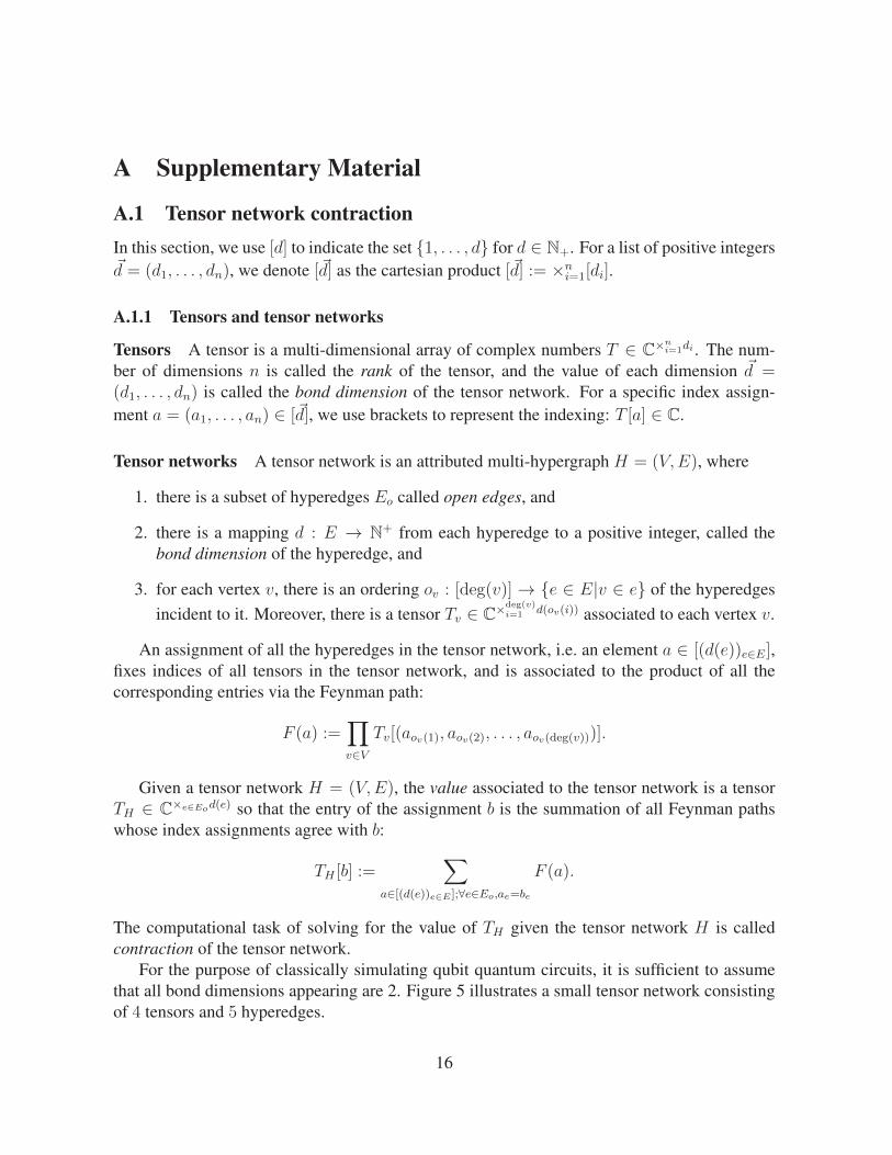
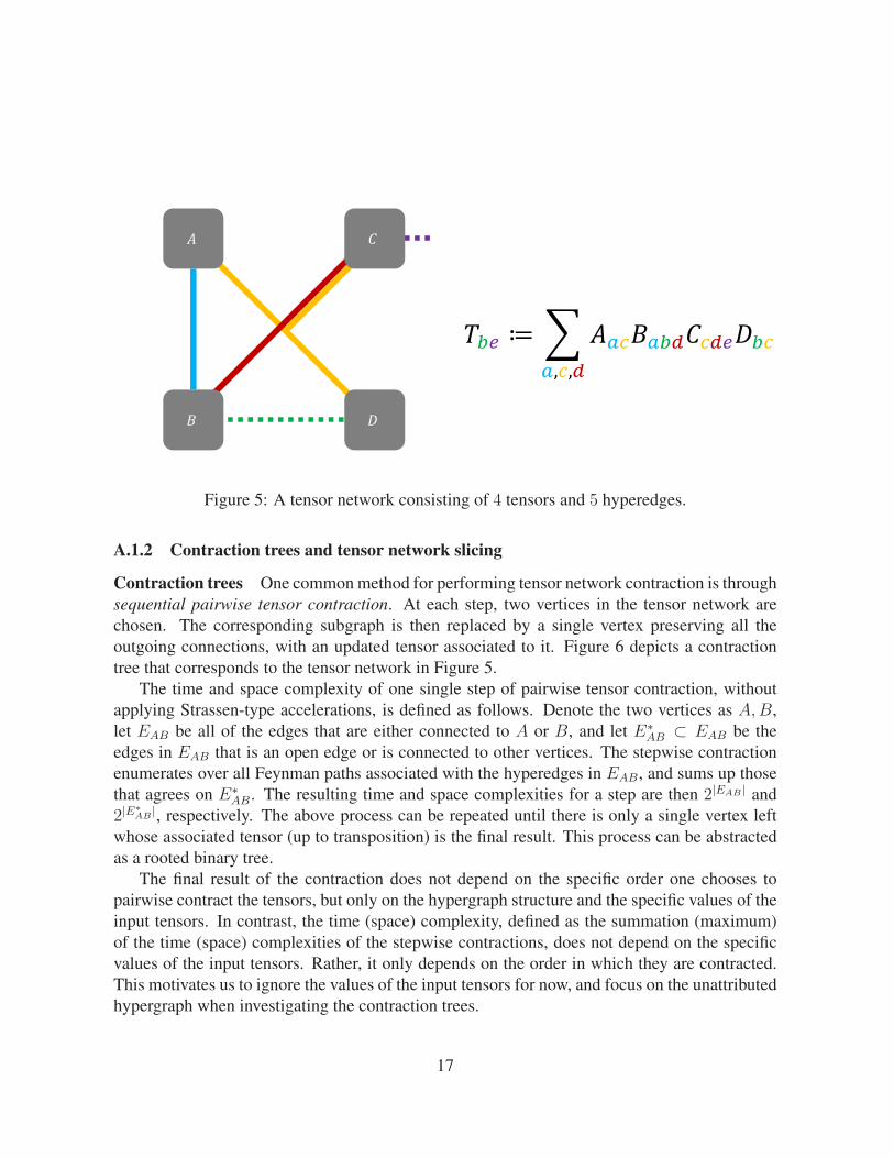
For the purpose of classically simulating qubit quantum circuits, it is sufficient to assumethat all bond dimensions appearing are 2. Figure 5 illustrates a small tensor network consistingof 4 tensors and 5 hyperedges.

16

!

" #

$

!!" ≔ ##,%,&

$#%%#!&&%&"'!%

Figure 5: A tensor network consisting of 4 tensors and 5 hyperedges.

A.1.2 Contraction trees and tensor network slicing

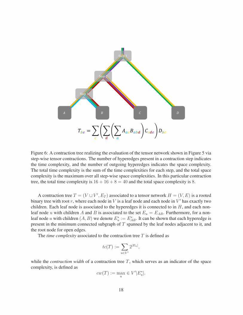
Contraction trees One common method for performing tensor network contraction is throughsequential pairwise tensor contraction. At each step, two vertices in the tensor network arechosen. The corresponding subgraph is then replaced by a single vertex preserving all theoutgoing connections, with an updated tensor associated to it. Figure 6 depicts a contractiontree that corresponds to the tensor network in Figure 5.

The time and space complexity of one single step of pairwise tensor contraction, withoutapplying Strassen-type accelerations, is defined as follows. Denote the two vertices as A,B,let EAB be all of the edges that are either connected to A or B, and let E∗AB ⊂ EAB be theedges in EAB that is an open edge or is connected to other vertices. The stepwise contractionenumerates over all Feynman paths associated with the hyperedges in EAB, and sums up thosethat agrees on E∗AB. The resulting time and space complexities for a step are then 2|EAB | and2|E

∗AB |, respectively. The above process can be repeated until there is only a single vertex left

whose associated tensor (up to transposition) is the final result. This process can be abstractedas a rooted binary tree.

The final result of the contraction does not depend on the specific order one chooses topairwise contract the tensors, but only on the hypergraph structure and the specific values of theinput tensors. In contrast, the time (space) complexity, defined as the summation (maximum)of the time (space) complexities of the stepwise contractions, does not depend on the specificvalues of the input tensors. Rather, it only depends on the order in which they are contracted.This motivates us to ignore the values of the input tensors for now, and focus on the unattributedhypergraph when investigating the contraction trees.

17

! " #$

Step 1

Step 2

Step 3

!!" =##

#$

#%$%#%%!$ &#$" '!#

Figure 6: A contraction tree realizing the evaluation of the tensor network shown in Figure 5 viastep-wise tensor contractions. The number of hyperedges present in a contraction step indicatesthe time complexity, and the number of outgoing hyperedges indicates the space complexity.The total time complexity is the sum of the time complexities for each step, and the total spacecomplexity is the maximum over all step-wise space complexities. In this particular contractiontree, the total time complexity is 16 + 16 + 8 = 40 and the total space complexity is 8.

A contraction tree T = (V ∪ V ′, ET ) associated to a tensor network H = (V,E) is a rootedbinary tree with root r, where each node in V is a leaf node and each node in V ′ has exactly twochildren. Each leaf node is associated to the hyperedges it is connected to in H , and each non-leaf node u with children A and B is associated to the set Eu = EAB. Furthermore, for a non-leaf node u with children (A,B) we denote E∗u := E∗AB. It can be shown that each hyperedge ispresent in the minimum connected subgraph of T spanned by the leaf nodes adjacent to it, andthe root node for open edges.

The time complexity associated to the contraction tree T is defined as

tc(T ) :=∑u∈V ′

2|Eu|,

while the contraction width of a contraction tree T , which serves as an indicator of the spacecomplexity, is defined as

cw(T ) := maxu∈ V ′|E∗u|.

18

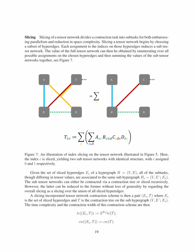
Slicing Slicing of a tensor network divides a contraction task into subtasks for both embarrass-ing parallelism and reduction in space complexity. Slicing a tensor network begins by choosinga subset of hyperedges. Each assignment to the indices on those hyperedges induces a sub ten-sor network. The value of the full tensor network can then be obtained by enumerating over allpossible assignments on the chosen hyperedges and then summing the values of the sub tensornetworks together, see Figure 7.

!!" ≔#%

##,&

$#%%#!&&%&"'!%

!

" #

$ !!

" #!

$!

=##

Figure 7: An illustration of index slicing on the tensor network illustrated in Figure 5. Here,the index c is sliced, yielding two sub tensor networks with identical structure, with c assigned0 and 1 respectively.

Given the set of sliced hyperedges Es of a hypergraph H = (V,E), all of the subtasks,though differing in tensor values, are associated to the same sub hypergraph Hs = (V,E \ Es).The sub tensor networks can either be contracted via a contraction tree or sliced recursively.However, the latter can be reduced to the former without loss of generality by regarding theoverall slicing as a slicing over the union of all sliced hyperedges.

A slicing-incorporated tensor network contraction scheme is then a pair (Es, T ) where Esis the set of sliced hyperedges and T is the contraction tree on the sub hypergraph (V,E \ Es).The time complexity and the contraction width of this contraction scheme are then

tc((Es, T )) := 2|Es|tc(T ),

cw((Es, T )) := cw(T ).

19

Real-world computational devices can usually work for long periods of time, but are re-stricted by memory. Therefore, the goal of finding a good contraction scheme can be formu-lated as minimizing the total time complexity subject to the constraint that the space complexityis bounded by a predetermined memory limit. For an Nvidia V100 with 16 GiB of memory,it is usually sufficient to slice the tensor network so that the contraction width is at most 29,assuming single precision.

A.2 Optimization methodsIn the following section, we describe the heuristics we use for obtaining a good contractionscheme. The heuristics are based on our observation that a typical contraction tree consistsof a stem of overwhelming cost, and short branches attached to that stem. See Figure 3 for aflowchart describing the algorithm.

A.2.1 Stems and branches

We first focus on finding good contraction trees without slicing indices. Since the total timecomplexity of a contraction tree is an exponential sum tc(T ) =

∑u∈V ′ 2

|Eu|, it is importantto understand how the cost is distributed across a typical contraction tree. We observe thatthe high-weight nodes in a contraction tree tend to form a path, as illustrated in Figure 1. Wecall this high-weight path the stem of the tree. Each node in this path has essentially the sameweight, while nodes outside this path typically have significantly smaller weights. Moreover,the nodes with smaller weights tend to form small clusters attached to the stem of the treewe call branches. Consequently, we focus on optimizing the stem of the contraction tree byreducing its thickness (the computational cost for each stem node) and its length (the numberof stem nodes) in order to minimize the total contraction cost.

A.2.2 Multi-parameter optimization based on hypergraph decomposition

Stem finding: hypergraph multipartite decomposition Inspired by [9], we use hypergraphdecompositions to first find the starting point of a stem. A K-wise hypergraph decompositionwith imbalance parameter ε decomposes the hypergraph into K parts such that the cut acrosseach part is minimized, subject to the constraint that each part contains at most (1 + ε)d |V |

Ke

vertices. It was shown in [9] that hypergraph decomposition-based contraction-finding algo-rithms are more efficient than previously proposed tree decomposition-based algorithms. Thisis because the cuts are more relevant to the space complexity of the contraction scheme thanthe treewidth, which is only the maximum time complexity of a single step. In practice, we findthat multipartite hypergraph decompositions work best at finding major components containingthe stem of the contraction. A hypergraph decomposition typically finds one major componentcontaining the stem, and occasionally it finds two major components each containing part of thestem, in the case that the root of the contraction tree lies in the middle of the stem.

20

Stem construction: recursive bipartite decomposition Once we find the major componentscontaining the stem, we can remove the branches one-by-one by recursively using hypergraphbipartitions. Setting an imbalance parameter ε′ close to 1 allows us to “peel off” one smallbranch at a time. This process can be repeated until the number of nodes left is fewer than apreset threshold N , at which point the stem is believed to have ended.

In our implementation, N is fixed to 25. The algorithm optimizes over the parameter set(K, ε, ε′) in order to find an optimal assignment of the parameters. We use the software pack-ages KaHyPar [30, 31] for hypergraph decomposition and CMA-ES [32] for parameter opti-mization. At the end, a batch of initial contraction trees are obtained from the best parameterset we found, which are then fed to further optimization and slicing routines described below.

A.2.3 Local optimization

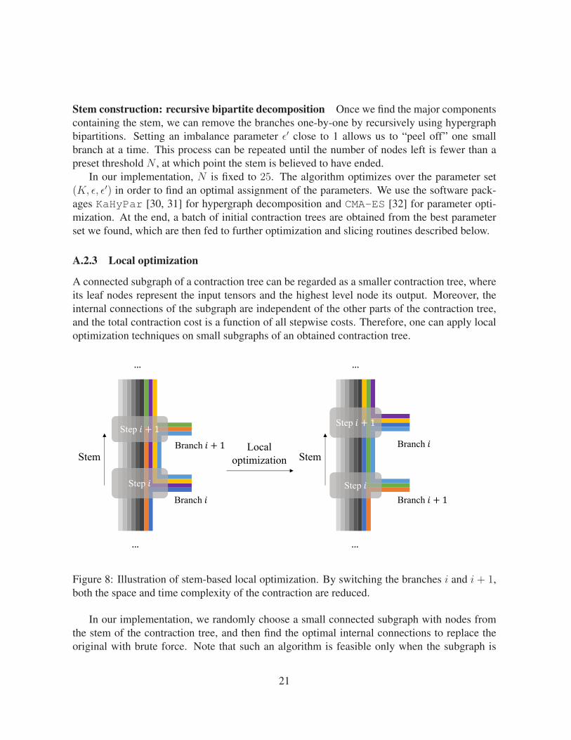
A connected subgraph of a contraction tree can be regarded as a smaller contraction tree, whereits leaf nodes represent the input tensors and the highest level node its output. Moreover, theinternal connections of the subgraph are independent of the other parts of the contraction tree,and the total contraction cost is a function of all stepwise costs. Therefore, one can apply localoptimization techniques on small subgraphs of an obtained contraction tree.

Step ! + 1

Step !

Stem

…

…

Branch !

Branch ! + 1

Step ! + 1

Step !

Stem

…

…

Branch ! + 1

Branch !

Localoptimization

Figure 8: Illustration of stem-based local optimization. By switching the branches i and i + 1,both the space and time complexity of the contraction are reduced.

In our implementation, we randomly choose a small connected subgraph with nodes fromthe stem of the contraction tree, and then find the optimal internal connections to replace theoriginal with brute force. Note that such an algorithm is feasible only when the subgraph is

21

sufficiently small. This process is repeated until no significant improvements are observed, or afixed number of iterations have passed.

A.2.4 Dynamic slicing

When the space complexity of the contraction tree is not small enough to fit into memory,slicing must be done. In our implementation, slicing is performed greedily so that each time ahyperedge is sliced, the total time complexity increases the least. Between two steps of pickingsliced indices, local optimization is applied to slightly restructure the contraction tree. Thishelps to increase the chance that the next sliced hyperedges will not increase the total timecomplexity significantly. In practice, we observed an ≈ .2% total increase in time complexityfor 10 hyperedges sliced, and about an ≈ 4× increase for 25 hyperedges sliced.

A.3 Runtime modification of the contraction schemeTo better accommodate the capability and limitations of the GPU, we further apply the followingruntime-specific modifications.

Pre-computation The branches of the contraction tree represent insignificant portions of theoverall time complexity. However, they involve many small tensors, transmission of which tothe GPU would incur significant overhead. Moreover, hyperedges involving branches usuallyhave very little intersection with the sliced hyperedges. This motivates us to pre-compute thebranches on a CPU before computing the stems of the individual tasks. The partial results forthe branches are shared by all subtasks and only need to be computed once. In practice, thissignificantly reduces the communication cost between the GPU and the CPU, and helps save asmall portion of computational cost.

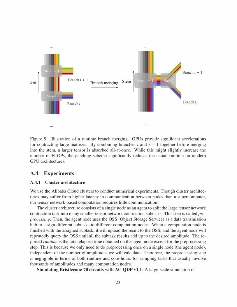
Branch merging The stem computation performed on the GPU is typically a sequential ab-sorption of small branch tensors into the large stem tensor, or two sides of the stem mergedtogether near the root. In either cases, a contraction tree with locally optimal contraction coststypically suffers from a large contrast in dimensions during matrix multiplication. On NvidiaTesla V100 GPUs, matrix multiplication with dimensions M × N and N × K is much moreefficient when the dimensions M,N and K are all multiples of 32. However, a typical branchtensor is often shaped as 4 × 4, 8 × 8, or 16 × 16. To overcome this, adjacent branches aremerged together to form a bigger tensor to contract with the stem, as depicted in Figure 9. Thisincreases the runtime contraction cost, but decrease the actual runtime by making use of theefficient kernel functions of the Nvidia Tesla V100. While this is an ad-hoc solution to the lowGPU-efficiency induced by small tensor dimensions, we hope that more systematic ideas couldbe incorporated to increase the GPU efficiency.

22

Step ! + 1

Step !

Stem Branch ! + 1

Branch !

...

...

Step ! + 1 Step !

Branch ! + 1

Branch !

Stem

...

...

Branch merging

Figure 9: Illustration of a runtime branch merging. GPUs provide significant accelerationsfor contracting large matrices. By combining branches i and i + 1 together before merginginto the stem, a larger tensor is absorbed all-at-once. While this might slightly increase thenumber of FLOPs, the patching scheme significantly reduces the actual runtime on modernGPU architectures.

A.4 ExperimentsA.4.1 Cluster architecture

We use the Alibaba Cloud clusters to conduct numerical experiments. Though cluster architec-tures may suffer from higher latency in communication between nodes than a supercomputer,our tensor network-based computation requires little communication.

The cluster architecture consists of a single node as an agent to split the large tensor networkcontraction task into many smaller tensor network contraction subtasks. This step is called pre-processing. Then, the agent node uses the OSS (Object Storage Service) as a data transmissionhub to assign different subtasks to different computation nodes. When a computation node isfinished with the assigned subtask, it will upload the result to the OSS, and the agent node willrepeatedly query the OSS until all the subtask results add up to the desired amplitude. The re-ported runtime is the total elapsed time obtained on the agent node except for the preprocessingstep. This is because we only need to do preprocessing once on a single node (the agent node),independent of the number of amplitudes we will calculate. Therefore, the preprocessing stepis negligible in terms of both runtime and core-hours for sampling tasks that usually involvethousands of amplitudes and many computation nodes.

Simulating Bristlecone-70 circuits with AC-QDP v1.1: A large-scale simulation of

23

12 14 16 18 20

1013

1014

1015

1016

1017

1018

1019

1020

Number of cycles m

Contractioncost

Figure 10: For each length, we run preprocessing for the quantum circuits in [14] five times. InFigure 4 we report the best contraction order we obtained over all five runs. Here, we report thecontraction cost for each run.

Bristlecone-70 circuits using double precision was conducted on an Alibaba Cloud cluster com-posed of 1449 Elastic Compute Service (ECS) instances, each with 88 Intel Xeon (Skylake)Platinum 8163 vCPU cores @ 2.5 GHz and 160 GiB of memory as computation nodes. We cal-culated 200, 000, 1, 000, 200, and 1 amplitudes of Bristlecone-70 circuits with depth 1+28+1,1 + 32 + 1, 1 + 36 + 1, and 1 + 40 + 1, respectively. The last two were the first successfulsimulations of instances at those depths. For the sake of comparison, we also created 4 ECSinstances with 2, 4, 8, and 16 vCPU cores, respectively, as part of a ‘virtual’ cluster of 127, 512vCPU cores. Those ECS instances supported Memory-to-CPU-core ratios of 2. For a largetensor network contraction task that has been split into K subtasks that each fit into 2 GiB ofmemory, we ran K

127,512subtasks on each vCPU core. We use the largest execution time on those

ECS instances to extrapolate the execution time of the whole tensor network contraction taskon the large cluster. Comparing the results, we concluded that scheduling and communication

24

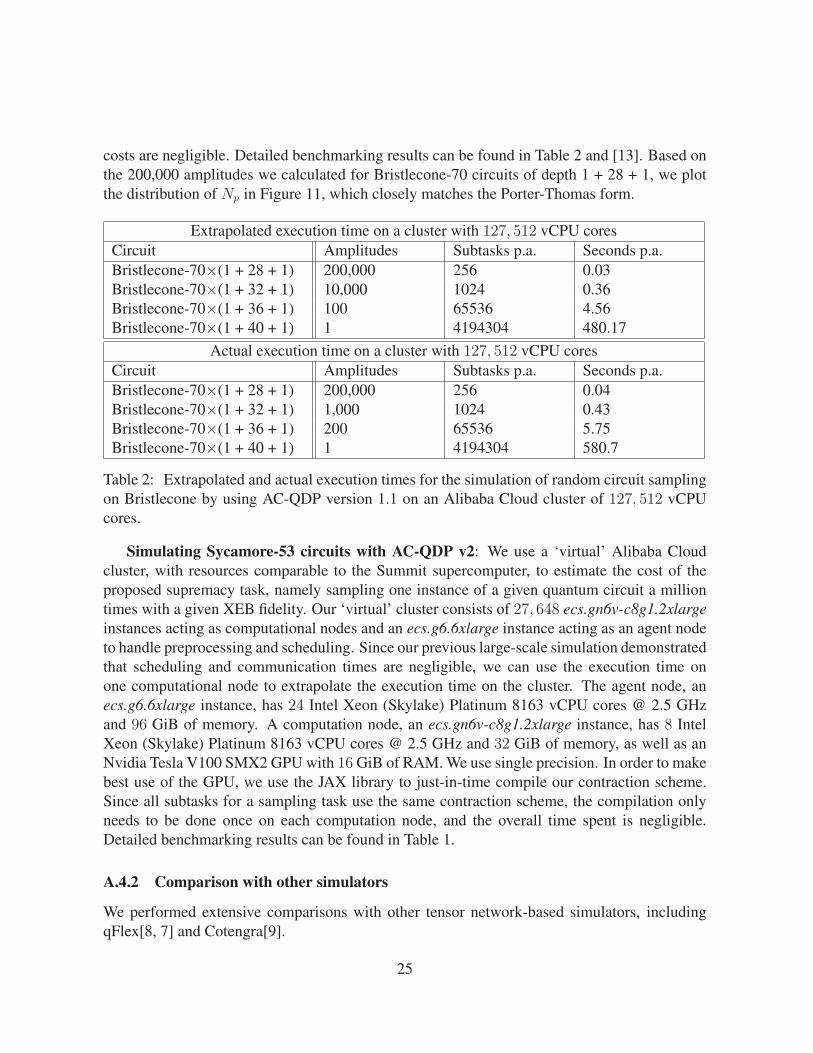
costs are negligible. Detailed benchmarking results can be found in Table 2 and [13]. Based onthe 200,000 amplitudes we calculated for Bristlecone-70 circuits of depth 1 + 28 + 1, we plotthe distribution of Np in Figure 11, which closely matches the Porter-Thomas form.

Extrapolated execution time on a cluster with 127, 512 vCPU coresCircuit Amplitudes Subtasks p.a. Seconds p.a.Bristlecone-70×(1 + 28 + 1) 200,000 256 0.03Bristlecone-70×(1 + 32 + 1) 10,000 1024 0.36Bristlecone-70×(1 + 36 + 1) 100 65536 4.56Bristlecone-70×(1 + 40 + 1) 1 4194304 480.17

Actual execution time on a cluster with 127, 512 vCPU coresCircuit Amplitudes Subtasks p.a. Seconds p.a.Bristlecone-70×(1 + 28 + 1) 200,000 256 0.04Bristlecone-70×(1 + 32 + 1) 1,000 1024 0.43Bristlecone-70×(1 + 36 + 1) 200 65536 5.75Bristlecone-70×(1 + 40 + 1) 1 4194304 580.7

Table 2: Extrapolated and actual execution times for the simulation of random circuit samplingon Bristlecone by using AC-QDP version 1.1 on an Alibaba Cloud cluster of 127, 512 vCPUcores.

Simulating Sycamore-53 circuits with AC-QDP v2: We use a ‘virtual’ Alibaba Cloudcluster, with resources comparable to the Summit supercomputer, to estimate the cost of theproposed supremacy task, namely sampling one instance of a given quantum circuit a milliontimes with a given XEB fidelity. Our ‘virtual’ cluster consists of 27, 648 ecs.gn6v-c8g1.2xlargeinstances acting as computational nodes and an ecs.g6.6xlarge instance acting as an agent nodeto handle preprocessing and scheduling. Since our previous large-scale simulation demonstratedthat scheduling and communication times are negligible, we can use the execution time onone computational node to extrapolate the execution time on the cluster. The agent node, anecs.g6.6xlarge instance, has 24 Intel Xeon (Skylake) Platinum 8163 vCPU cores @ 2.5 GHzand 96 GiB of memory. A computation node, an ecs.gn6v-c8g1.2xlarge instance, has 8 IntelXeon (Skylake) Platinum 8163 vCPU cores @ 2.5 GHz and 32 GiB of memory, as well as anNvidia Tesla V100 SMX2 GPU with 16 GiB of RAM. We use single precision. In order to makebest use of the GPU, we use the JAX library to just-in-time compile our contraction scheme.Since all subtasks for a sampling task use the same contraction scheme, the compilation onlyneeds to be done once on each computation node, and the overall time spent is negligible.Detailed benchmarking results can be found in Table 1.

A.4.2 Comparison with other simulators

We performed extensive comparisons with other tensor network-based simulators, includingqFlex[8, 7] and Cotengra[9].

25

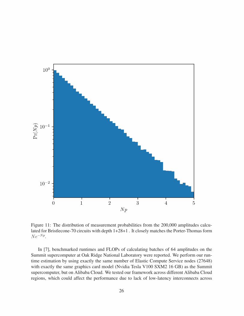
Figure 11: The distribution of measurement probabilities from the 200,000 amplitudes calcu-lated for Bristlecone-70 circuits with depth 1+28+1 . It closely matches the Porter-Thomas formNe−Np.

In [7], benchmarked runtimes and FLOPs of calculating batches of 64 amplitudes on theSummit supercomputer at Oak Ridge National Laboratory were reported. We perform our run-time estimation by using exactly the same number of Elastic Compute Service nodes (27648)with exactly the same graphics card model (Nvidia Tesla V100 SXM2 16 GB) as the Summitsupercomputer, but on Alibaba Cloud. We tested our framework across different Alibaba Cloudregions, which could affect the performance due to lack of low-latency interconnects across

26

regions. However, because our algorithm introduces very little communication, the communi-cation overhead is negligible.

In [9], benchmarked times and other information for computing single amplitudes of ran-dom circuits with single precision using Nvidia Quadro P2000s were reported. In order toconduct a fair comparison, we re-ran the latest GitHub version of Cotengra to calculate sin-gle amplitudes with perfect fidelity on the same Elastic Compute Service node with the samegraphics card (Nvidia Tesla V100 SXM2 16 GB) that we used to benchmark AC-QDP. In AC-QDP, the preprocessing step is controlled by the number of iterations in the CMA-ES algo-rithm and the number of iterations of local optimization. Consequently, there is no way toprecisely control the preprocessing time. However, by using the iteration parameters men-tioned above, it usually takes from one hour to several hours, depending on number of cy-cles. To avoid underestimating Cotengra and to better understand its ultimate capability, weallow the path optimizer in Cotengra to search for 10 hours, which should always be largeenough to compare with the pre-processing time used in the AC-QDP benchmark. As con-tracting open tensor networks has not been implemented in the latest version of Cotengra onGitHub (949635c6783435fc384553ec28c7c038dc786e01), we use the runtime reported for asingle amplitude calculation as a lower bound for a 64-amplitude batch calculation. We thenuse the runtime of a single-amplitude calculation to estimate the cost of frugal rejection sam-pling with 10× overhead as an upper bound for the sampling task [24].

We also compare AC-QDP with the classical algorithms proposed in [7]. Since both aretargeting the same sampling task by assuming Summit-comparable computational resources,we use the numbers reported in [7].

The simulation proposal in [10] leverages secondary storage to assist main memory whenthe quantum state is too large to fit. Any proposal that needs to store the entire state vector islimited by the storage space available. The Summit supercomputer has 250 PiB of secondarystorage, while a 54-qubit state vector stored in single precision takes 128 PiB to store. Thespace requirement doubles with each additional qubit, and so this proposal would already havetrouble scaling to 55-qubit circuits, while 56-qubit circuits would be out of reach.

The time estimate in [10] is based on the runtimes reported in [11], in which 0.5 PiB ofmemory were used to support a double-precision simulation of a 45-qubit quantum circuit onthe Cori II supercomputer. The simulation makes use of highly optimized CPU kernels, whichare not applicable to Summit, a supercomputer with most of its computational power in GPUs.Furthermore, [10] scales the runtime down based on LINPACK benchmark figures for Cori IIand Summit, making two implicit assumptions. First, the CPU kernels in [11] that are highlyoptimized for the task of quantum simulation are portable to GPUs with no loss in efficiency.Second, the LINPACK benchmark figures, which allow the user to choose the most suitableproblem size for a given machine, are applicable to the specific task that [11] performs on asingle node: simulating up to 32 local qubits. This is problematic given that each socket (theSummit equivalent of a node in [10]) only has 16 × 3 = 48 GiB of GPU memory among its 3GPUs, while data transfer to and from the GPU can be quite expensive.

For comparison, we estimated the theoretical runtime of our simulator for the 20-cycle quan-

27

tum supremacy task under two analogous assumptions. First, a further optimized implementa-tion should achieve a GPU FLOPS efficiency comparable to Cotengra, a simulator fundamen-tally similar to ours. In 18- and 20-cycle experiments on V100 GPUs, we observe a GPUefficiency in excess of 90% with respect to the single-precision performance figure of 15.7 ter-aFLOPS. Second, we assume that tensors of rank 32 can be contracted on GPUs, presumablyusing out-of-core memory access, without a significant loss in efficiency. We would then onlyneed to slice enough indices to decrease the contraction width to 32, for which we found acontraction scheme with total cost 1018.6. Combining both assumptions yields the estimate

(8× 1018.6) FLOPs/sample15.7× 1012 FLOPS× 90%× 27648

× 2000 samples ≈ 1.63× 105 seconds ≈ 1.89 days.

28