1

Frank L. H. Wolfs Department of Physics and Astronomy, University of Rochester, Slide 1

Classical MechanicsPhy 235, Lecture 04.

Frank L. H. WolfsDepartment of Physics and Astronomy

University of Rochester

1

Frank L. H. Wolfs Department of Physics and Astronomy, University of Rochester, Slide 2

Nothing to do with air planes, nothing to with PHY 235, just a nice picture of part of my group.

2

Frank L. H. Wolfs Department of Physics and Astronomy, University of Rochester, Slide 3

Extra Credit Homework Assignment.Study projectile motion.

• There are three extra credithomework assignments.

• Each assignment will requirenumerical simulations.

• Each assignment will have thesame weight as a regularassignment.

• You can thus earn 130%credit for the Phy 235homework component of yourfinal grade.

Physics 235 Due: noon, September, 25, 2020 Extra Credit Homework Set 01

- 1 -

Physics 235, Extra Credit Homework Set 01

Write the following text on the front cover of your homework assignment and sign it. If the text is missing, 20 points will be subtracted from your homework grade.

Consider the simulation of projectile motion, demonstrated in lecture 2. The script of this simulation can be found at the following URL:

https://www.glowscript.org/#/user/wolfs/folder/Public/program/ProjectileMotionChapter2 a) First consider pure projectile motion in vacuum (turn the dragg force off and set the

angle to 60°). Compare the difference between the analytical solution and the numerical solution as function of stepsize dt. Make a plot of this difference as function of dt. Based on this plot, determine an optimum value of dt to run the simulation. Note: you need to make sure you pick the proper range of dt values.

b) Repeat the study carried out in part a) for two different launch angles (45° and 30°) and

determine if your optimum choice of dt is angle dependent. c) Now turn on the drag force (k = 0.005) and set the launch angle to 60°. When we

include the drag force, we can no longer compare obtain an analytical solution and we have to determine the optimum dt in a different way. One possible approach is to look at the point of impact and determine how the point of impact depends on dt. Make a graph of the impact point as function of dt. Based on this plot, determine an optimum value of dt to run the simulation. Note: you need to make sure you pick the proper range of dt values.

3

2

Frank L. H. Wolfs Department of Physics and Astronomy, University of Rochester, Slide 4

Outline

• Damped and driven harmonic motion:• Damped harmonic motion occurs when friction or drag forces areacting on the system. Energy is dissipated and the system willgradually come to rest.

• Driven harmonic motion adds a driving force in order to compensatefor damping losses.

4

Frank L. H. Wolfs Department of Physics and Astronomy, University of Rochester, Slide 5

Solving Second-Order Differential Equations.Damped and driven.

• General form:

• If you find two linearly independent solutions, every other solution willbe a linear combination of these two solutions.• The general solution has two constants, defined by the initial conditions.

• Homogeneous equation:• f(x) is equal to 0.

• Inhomogeneous equation:• f(x) is not equal to 0.

d 2ydx2

+ a dydx

+ by = f (x)

5

Frank L. H. Wolfs Department of Physics and Astronomy, University of Rochester, Slide 6

Homogeneous Equation:

• Three different scenarios:• a2 > 4b

• a2 = 4b

• a2 < 4b

d 2ydx2

+ a dydx

+ by = 0

6

3

Frank L. H. Wolfs Department of Physics and Astronomy, University of Rochester, Slide 7

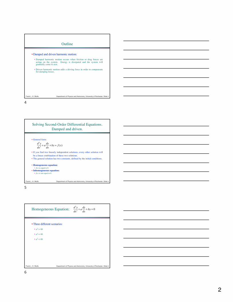
Inhomogeneous Equation:

• Suppose:• v is a solution of the inhomogeneous equation.

• u is the general solution of the homogeneous equation.

• Then:

• u + v is the general solution of the inhomogeneous equation.

d 2ydx2

+ a dydx

+ by = f (x)

7

Frank L. H. Wolfs Department of Physics and Astronomy, University of Rochester, Slide 8

Homogeneous Equation• Consider a damping force –bv and a restoring force –kx.

The equation of motion for such system is:ma = –bv – kx.• This provides us with the homogeneous equation:

• Try the following solution: x = ert.• Valid solution if r2 + 2br +w02 = 0:

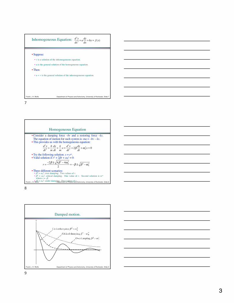
• Three different scenarios:• b2 > w0

2: over damping. Two values of r.• b2 = w0

2: critical damping. One value of r. Second solution is testwhere s = -b.• b2 < w0

2: under damping. Two values of r.

d 2xdt 2

+ bmdxdt

+ kmx = d

2xdt 2

+ 2β dxdt

+ω 02x = 0

r =−2β ± 4β 2 − 4ω 0

2

2= −β ± β 2 −ω 0

2

8

Frank L. H. Wolfs Department of Physics and Astronomy, University of Rochester, Slide 9

Damped motion.

9

4

Frank L. H. Wolfs Department of Physics and Astronomy, University of Rochester, Slide 10

Numerical studies.

• Using tools such as VPython, it is easy to explore howdamped harmonic motion changes as the dampingconditions are changed.

• Let us have a look:

http://www.glowscript.org/#/user/wolfs/folder/Public/program/DampedHarmonicMotion

10

Frank L. H. Wolfs Department of Physics and Astronomy, University of Rochester, Slide 11

Problem 3.22

• Let the initial position and speed of an overdamped, non-driven oscillator be x0 and v0, respectively.• Determine the values of the amplitudes A1 and A2 in equation 3.44.

11

Frank L. H. Wolfs Department of Physics and Astronomy, University of Rochester, Slide 12

3 Minute 12 Second Intermission.

• Since paying attention for 1hour and 15 minutes is hardwhen the topic is physics,let’s take a 3 minute 12second intermission.

• You can:• Stretch out.• Talk to your neighbors.• Ask me a quick question.• Enjoy the fantastic music.

12

5

Frank L. H. Wolfs Department of Physics and Astronomy, University of Rochester, Slide 13

Inhomogeneous Equation

• Consider a damping force –bv, a restoring force –kx, and adriving force f(t). The equation of motion for such systemis:ma = –bv – kx + f(t).

• The equation of motion becomes:

• Suppose:• v is a solution of the inhomogeneous equation (this is called theparticular solution).• u is the general solution of the homogeneous equation (this is calledthe complementary solution).

then:• u + v is the general solution of the inhomogeneous equation.

d 2xdt 2

+ bmdxdt

+ kmx = d

2xdt 2

+ 2β dxdt

+ω 02x = f t( )

13

Frank L. H. Wolfs Department of Physics and Astronomy, University of Rochester, Slide 14

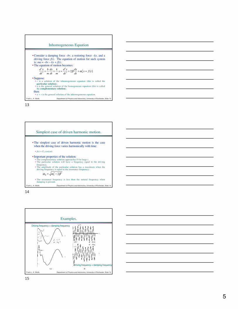
Simplest case of driven harmonic motion.

• The simplest case of driven harmonic motion is the casewhen the driving force varies harmonically with time:• f(t) = F0 cos(wt)

• Important properties of the solution:• The complementary solution approaches 0 for large t.• The particular solution will have a frequency equal to the drivingfrequency.• The amplitude of the particular solution has a maximum when thedriving frequency is equal to the resonance frequency:

• The resonance frequency is less than the natural frequency whendamping is present.

ω R = ω 02 − 2β 2

14

Frank L. H. Wolfs Department of Physics and Astronomy, University of Rochester, Slide 15

Examples.

Driving frequency > damping frequency

Driving frequency < damping frequency

15

6

Frank L. H. Wolfs Department of Physics and Astronomy, University of Rochester, Slide 16

Numerical studies.

• Using tools such as VPython, it is easy to explore howdriven harmonic motion changes as the driving conditionsare changed.

• Let us have a look:

http://www.glowscript.org/#/user/wolfs/folder/Public/program/DrivenHarmonicMotion

16

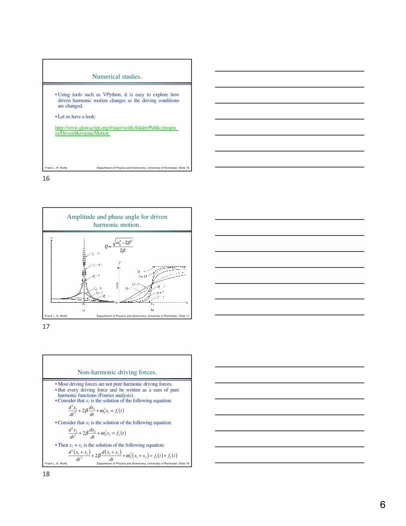
Frank L. H. Wolfs Department of Physics and Astronomy, University of Rochester, Slide 17

Amplitude and phase angle for driven harmonic motion.

Q=ω02−2β 2

2β

17

Frank L. H. Wolfs Department of Physics and Astronomy, University of Rochester, Slide 18

Non-harmonic driving forces.

• Most driving forces are not pure harmonic driving forces.• But every driving force and be written as a sum of pure

harmonic functions (Fourier analysis).• Consider that x1 is the solution of the following equation:

• Consider that x2 is the solution of the following equation:

• Then x1 + x2 is the solution of the following equation:

d 2x1dt 2

+ 2β dx1dt

+ω 02x1 = f1 t( )

d 2x2dt 2

+ 2β dx2dt

+ω 02x2 = f2 t( )

d 2 x1 + x2( )dt 2

+ 2βd x1 + x2( )

dt+ω 0

2 x1 + x2( ) = f1 t( )+ f2 t( )

18

7

Frank L. H. Wolfs Department of Physics and Astronomy, University of Rochester, Slide 19

Non-harmonic driving forces.

• If the function F has a period t, then we can write F as:

• For each term in this series, we can find the solution to thecorresponding inhomogeneous equation.

• The total solution is then the linear sum of all of theseindividual solutions.

F t( ) = 12a0 + an cos nωt( )+ bn sin nωt( )( )

n=1

∞

∑

ω = 2πτ

19

Frank L. H. Wolfs Department of Physics and Astronomy, University of Rochester, Slide 20

Example of Fourier Analysis.

F t( ) = 12a0 + an cos nωt( )+ bn sin nωt( )( )

n=1

∞

∑a0 = 0an = 0

20

Frank L. H. Wolfs Department of Physics and Astronomy, University of Rochester, Slide 21

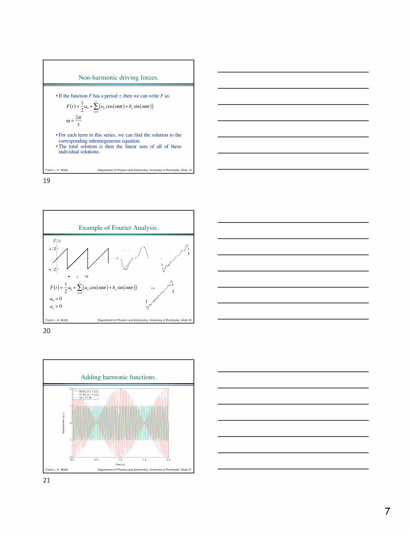
Adding harmonic functions.

-2

-1

0

1

2

Disp

lace

men

t (a

.u.)

2.01.51.00.50.0

Time (s)

30 Hz, A = 1 a.u. 31 Hz, A = 1 a.u. 30 + 31 Hz

21

8

Frank L. H. Wolfs Department of Physics and Astronomy, University of Rochester, Slide 22

ENOUGH FOR TODAY?

22