CLASSICAL HURWITZ NUMBERS AND RELATED · CLASSICAL HURWITZ NUMBERS AND RELATED COMBINATORICS 605 top coe cient" refer to the asymptotic growth of the elements of the sequence in question

MOSCOW MATHEMATICAL JOURNALVolume 17, Number 4, October–December 2017, Pages 601–633

CLASSICAL HURWITZ NUMBERS AND RELATED

COMBINATORICS

BORIS DUBROVIN, DI YANG, AND DON ZAGIER

To the memory of the extraordinary mathematician and man

Vladimir Igorevich Arnold,with admiration

Abstract. We give a polynomial-time algorithm of computing the clas-sical Hurwitz numbers Hg,d, which were defined by Hurwitz 125 yearsago. We show that the generating series of Hg,d for any fixed g > 2 livesin a certain subring of the ring of formal power series that we call theLambert ring. We then define some analogous numbers appearing inenumerations of graphs, ribbon graphs, and in the intersection theoryon moduli spaces of algebraic curves, such that their generating seriesbelong to the same Lambert ring. Several asymptotics of these numbers(for large g or for large d) are obtained.

2010 Math. Subj. Class. Primary: 14N10; Secondary: 16T30, 53D45, 05A15.

Key words and phrases. Hurwitz numbers, Lambert ring, Pandharipande’s

equation, enumerative geometry.

In 1891 Hurwitz [30] studied the number Hg,d of genus g > 0 and degree d > 1coverings of the Riemann sphere with 2g + 2d − 2 fixed branch points and in par-ticular found a closed formula for Hg,d for any fixed d. These Hurwitz numbers arenow very famous and have been studied from many different points of view (matrixmodels, Gromov–Witten invariants, topological recursion, classical/quantum inte-grable systems, . . . ); see for example [4], [7], [10], [12], [27], [28], [42], [43]. In thispaper we study their combinatorial properties, and compare them with some otherenumerative problems.

Introduce the following generating series of Hg,d

H = H(x, y) =∑g>0

∑d>1

hg,d x2g+2d−2 yd, hg,d :=

Hg,d

(2g + 2d− 2)!. (1)

In the first part of the paper (Section 1), which is completely elementary, we willdeduce from a recursion relation obtained by R. Pandharipande in [43] a muchsimpler one, which can be written compactly in terms of the generating series (1)

Received March 20, 2017; in revised form June 30, 2017.

c©2017 Independent University of Moscow

601

602 B. DUBROVIN, D. YANG, AND D. ZAGIER

in the following form

H(3) −H(2) = 2H(2)∞∑`=1

x2`

(2`)!H(2`+1),

H(n) :=(y∂

∂y

)nH =

∑g>0

∑d>1

dnhg,d x2g+2d−2 yd,

(2)

and use it to give simpler derivations of some known and new properties of Hg,d.In particular:

P1. For any fixed d > 1, the function Hg,d is a linear combination of finitely many

exponentials m2g+2d−2, 1 6 m 6(d2

), with coefficients in 2d!−2Z. For example, for

d = 6

6!2

2Hg,6 = 15w − 36 · 10w + 25 · 9w − 225 · 7w + 700 · 6w − 720 · 5w

+ 7200 · 4w − 15200 · 3w − 34200 · 2w + 163575,

where w = 2g + 10. (This example was already given by Hurwitz). In particular,we have the asymptotic formula

Hg,d ∼2

d!2

(d

2

)2g+2d−2

as g →∞. (3)

The exponential polynomials H∗,d can be computed recursively in time polynomialin d.

P2. For any fixed g > 0, the function d!hg,d belongs to the rank 2 module overQ[d] generated by the two integer-valued functions

d 7→ 2 dd−3 and d 7→ (d− 1)!

d−1∑r=0

dr

r!

and hg,d itself is a linear combination of h0,d and h1,d with polynomial coefficients,e.g.,

h2,d =7d4(d− 1)

4320h0,d −

5d2

72h1,d,

h3,d = −d4(d− 1)(99845d2 − 454d+ 24)

1045094400h0,d

+d2(128625d3 + 546700d2 − 980d+ 48)

174182400h1,d.

(4)

Moreover, the series H(n)g (z) =

∑d>1 hg,d d

nzd is a polynomial with rational coef-

ficients in H(3)0 (z) for all g and n satisfying the stability condition 2g − 2 + n > 0,

and there is a polynomial time (in g and n) recursive algorithm to compute thesepolynomials.

P3. The asymptotic behavior of Hg,d for g > 0 fixed is given by

Hg,d ∼cg√π/2

(24√

2)g Γ( 5g−12 )

(4

e

)dd2d−5+9g/2 as d→∞ (5)

CLASSICAL HURWITZ NUMBERS AND RELATED COMBINATORICS 603

or equivalently

hg,d ∼cg√

2

(96√

2)g Γ( 5g−12 )

d(5g−7)/2 ed as d→∞, (6)

where the numbers

c0 = −1, c1 = 2, c2 = 98, c3 = 19600, c4 = 8824802, c5 = 7061762400, . . .

are given by the recursion

cg = 50 (g − 1)2 cg−1 +1

2

g−2∑h=2

ch cg−h (g > 3) (7)

or equivalently by the statement that the generating series

U = U(X) =∑g>0

cgX12−

5g2

satisfies the Painleve I equation

d2U

dX2+

1

16U2 − 1

16X = 0. (8)

We indicate briefly which of these results were known and what is new. Thefirst statement of P1 is due to Hurwitz, as already mentioned, and the asymptoticformula (3) follows immediately, but the last statement is new. (Hurwitz’s formulasforH∗,d involve summations over all permutations or all partitions of d and thereforecontain an exponentially growing number of terms.) The first statement in P2seems not to be in the literature. The second statement, that every hg,∗ is a linearcombination of h0,∗ and h1,∗ with polynomial coefficients is implicit in the work ofGoulden, Jackson and Vakil [28]. However, the explicit computations were donethere only up to genus 3 (Examples 4.1–4.3), and actual formulas for higher generawould be almost impossible to obtain by their approach, which is based on difficultcomputations of Hodge integrals, whereas with our polynomial-time algorithm givenhere one can easily compute up to much larger values of the genus. The formula forh3,d given in [28] expresses it as a linear combination with polynomial coefficientsof h1,d and h2,d (one sees from (4) that this is possible, since the coefficient of h0,d

in h3,d is divisible by the coefficient of h0,d in h2,d) and a remark given by theauthors in this context (“This is to be expected to persist for g > 2,” p. 578) seemsto suggest that more generally hg,d is a combination with coefficients in Q[d] ofhg−1,d and hg−2,d for any g, but in fact this fails already for g = 4. (Of coursehg,d is always a combination of hg−1,d and hg−2,d with coefficients in Q(d), but ingeneral the coefficients will have denominators.) Finally, a result equivalent to P3was proved by Caporaso et al. [6] as a consequence of the Ekedahl–Lando–Shapiro–Vainshtein formula [21] along with Itzykson–Zuber’s result [32] on the asymptoticsof certain Gromov–Witten invariants of a point, whereas we give a direct proofusing just the recursion.

We also remark that to obtain the results of P2 we study two simple spacesof sequences of rational numbers (the “Lambert space” and “extended Lambertspace”) that contain the sequences d 7→ d!hg,d with g fixed and many other in-teresting counting functions. Related spaces have appeared in the literature many


times, most notably in [46], but our way of studying these spaces and several of thespecific results that we prove about them are new.

The second part of this paper (Section 2), describes a different method of com-puting Hg,d for fixed g based on the Dubrovin–Zhang (DZ) approach [18]. It wasshown by Pandharipande [43] that Hg,d are special Gromov–Witten (GW) invari-ants of the complex projective line P1. In [9], [18], [11], the first named author andY. Zhang developed a powerful method of computing GW invariants of any smoothprojective variety with semisimple quantum cohomology. The quantum cohomol-ogy of P1 is semisimple. Indeed, the small quantum cohomology of P1 at the originis already semisimple:

1 ? 1 = 1, 1 ? ω = ω ? 1 = ω, ω ? ω = 1, (9)

where 1 ∈ H0(P1; Q), ω ∈ H2(P1; Q) is the Poincare dual of a point, and ? denotesthe quantum product. Hence one can apply the DZ approach to the computation ofHg,d. We mention that, according to [9], [18], the multiplication table (9) togetherwith the Poincare paring on H∗(P1; Q) contain complete information on all GWinvariants of P1.

In the third part of this paper (Section 3), we investigate three more modelsin enumerative geometry that share similar properties with Hurwitz’s countingproblem. The first one is the enumeration of ordinary graphs. The second one is theenumeration of ribbon graphs (aka Grothendieck’s dessins d’enfants) [3], [29], [36].Although closed formulas for the enumeration of ribbon graphs with one and twovertices had been obtained in [29] and [38], respectively, it is only recently that twoefficient algorithms for the ribbon graph enumeration (one is efficient for large genus,the other is efficient for large number of vertices) have been developed by two of theauthors [16], [17]. The algorithm in [17] observes an interesting relationship betweenHodge integrals and matrix integrals called the Hodge–GUE correspondence. Thevalidity of this algorithm has been proved very recently in [14]. The third one is thestudy of intersection numbers (of the so-called ψ-classes) over the Deligne–Mumfordmoduli space Mg,n of stable algebraic curves of genus g with n distinct markedpoints along with nonlinear Hodge classes of the most general type [39], [23], [13].The comparisons between these three models and Hurwitz’s problem with g > 2are summarized in the following list:

order of the mostsingular term

characterization ofthe top coefficient

Ordinary graphs 3g − 3 Riccati equationRibbon graphs 4g − 4 not knownHodge integrals 5g − 5 Painleve I equationHurwitz numbers 5g − 5 Painleve I equation

Here, for Hurwitz’s problem, g is the genus of the upper Riemann surface of acovering; for Hodge integrals, g is the genus of the stable curves that form themoduli space; for an ordinary graph, g is the number of loops of the graph; for aribbon graph, g is defined as the smallest genus of a Riemann surface into whichthe ribbon graph can be embedded, while the words “most singular term” and “the


top coefficient” refer to the asymptotic growth of the elements of the sequence inquestion for fixed g.

1. Elementary Theory of Hurwitz Numbers

In this section we derive the main combinatorial properties of the Hurwitz num-bers from a completely elementary point of view, not involving any geometric con-siderations. Our main tool is a quadratic recursion that we give in Section 1.1. Thediscussions of the Hurwitz numbers for fixed d or fixed g are given in Sections 1.2and 1.3, respectively, while Sections 1.4 and 1.5 discuss the Lambert space and theasymptotic properties of the Hurwitz numbers.

1.1. A quadratic recursion for the Hurwitz numbers. It was conjectured byPandharipande [43] and later proved by Okounkov [40] that the generating seriesH defined in (1) satisfies the following differential-functional equation

D2H(x, y) = y eH(x,yex)−2H(x,y)+H(x,ye−x), D := y∂

∂y. (10)

Expanding H(x, y e±x) by Taylor’s theorem and comparing the coefficients of bothsides, one can rewrite (10) equivalently as a recursion for the numbers hg,d =Hg,d/(2g + 2d− 2)! (page 64 of [43]):

hg,d =1

d2

∞∑`=0

2`

`!

∑d1,...,d`>1∑di=d−1

∑g1,...,g`>0k1,...,k`>1∑(gi+ki−1)=g

∏i=1

d2ki

(2ki)!hgi,di . (11)

Our first observation is that both (10) and (11) can be replaced by much simplerquadratic equations.

Proposition 1. The generating series H satisfies the differential-functional equa-tion

D3H(x, y)−D2H(x, y)

= D2H(x, y)(DH(x, y ex)− 2DH(x, y) +DH(x, y e−x)

). (12)

Equivalently, the numbers hg,d = Hg,d/(2g + 2d− 2)! are given recursively by

hg,d =2

d2(d− 1)

∑d1,d2>1d1+d2=d

∑g1,g2>0, `>1g1+g2+`=g+1

d2`+11 d2

2

(2`)!hg1,d1hg2,d2 . (13)

Proof. Equation (12) follows from (10) by applying D to both sides, and (13)from (12).

The quadratic recursion (13) is useful not only for theoretical considerations, aswe will see in the rest of this section, but also for numerical purposes, since thenumber of terms on the right grows only polynomially (like O(g2d)) rather thanexponentially in the arguments g and d.


1.2. Hurwitz numbers for fixed degree. Our first application of Proposition 1is to study the numbers hg,d for fixed d by giving a recursive formula for thegenerating functions

Cd(x) :=∑g>0

hg,d x2g−2+2d (d > 1).

This also gives a convenient algorithm for computing the Hurwitz numbers, sincethe recursion for Cd involves only O(d) terms, so that we can easily calculate up tofairly large values of d.

To state the recursion we will use a sequence of polynomials Pk = Pk(s), withinitial values

P1 = s, P2 = s2 + 4s, P3 = s3 + 6s2 + 9s, P4 = s4 + 8s3 + 20s2 + 16s, . . . ,

that can be defined either by Pk(s) = 2Tk(s+2

2

)− 2 (Tk = Chebyshev polynomial

of the first kind) or else recursively by Pk+1 = (s + 2)Pk − Pk−1 + 2s, or else in

closed form as∑ki=1

((k+i2i

)+(k+i−1

2i

))si. (The equivalence of these three definitions

is elementary.) Then we have:

Theorem 1. The generating series Cd(x) ∈ Q[[x]] is given for each d > 1 by

Cd(x) =1

dγd(4 sinh2(x/2)

), (14)

where γd(s) is a polynomial of degree(d2

)in s defined inductively by

γd(s) =1

d2 − d

d−1∑k=1

(d− k)Pk(s) γk(s) γd−k(s) (d > 2) (15)

together with the initial condition γ1(s) = 1, the first values being

γ1(s) = 1, γ2(s) =s

2! 1!, γ3(s) =

s3 + 6s2

3! 2!, γ4(s) =

s6 + 12s5 + 54s4 + 96s3

4! 3!, . . . .

Proof. Since H =∑d Cd(x)yd, we have

DH(x, y ex)− 2DH(x, y) +DH(x, y e−x) =∑d>1

dCd(x)(edx − 2 + e−dx)yd. (16)

Using (16) and comparing coefficients of yd of the both sides of (12) we find

(d3 − d2)Cd(x) =

d−1∑k=1

k(d− k)2(ekx − 2 + e−kx)Ck(x)Cd−k(x). (17)

After changing variables from x to s = 4 sinh2(x/2) (and also multiplying Cd by dto simplify the recursion slightly), this takes the form (15) with Pk(s) defined byPk(x − 2 + x−1) = xk − 2 + x−k, which is equivalent to each of the definitions ofPk given just before the theorem.

Remark. Although equation (12) in Proposition 1 follows easily from Pandhari-pande’s equation, it changes considerably the form of the recursion for Hg,d, andsignificantly reduces the time complexity. This is actually an unexpected phenom-enon, essentially due to the nonlinearity of Pandharipande’s original equation (10).


To the best of our knowledge, the algorithm described in Theorem 1 is the first onein the literature with the polynomial time complexity for computing Hg,d. See inSections 1.5 and 1.3 for more discussions as well as applications.

The following corollary is a more precise version of the statement P1 of theintroduction.

Corollary (Hurwitz 1891). The numbers Hg,d for fixed d have the form

Hg,d =2

d!2

∑16m6(d2)

bd,mm2g+2d−2, (18)

where bd,m are integers with bd,(d2)= 1 and bd,m = 0 for

(d−1

2

)< m <

(d2

).

Proof. From Proposition 1 or from the recursion (17) we see that Cd(x) is a Laurentpolynomial in ex and is even in x. This implies a formula of the form (18) with

bd,m ∈ Q. The further properties (integrality and values for m >(d−1

2

)) are also

easily deduced from (17).

We end this subsection by discussing another approach to calculating the num-bers Hg,d and proving the corollary above that was discovered by Hurwitz himselfin a second paper [31] in 1901. Let H∗k,d be the weighted (by inverse number of

automorphisms) number of (not necessarily connected) coverings of P1 of degree dwith k simple ramification points, and introduce the corresponding generating series

ZH = ZH(x, y) :=∑k, d>0

H∗k,dk!

xkyd =:∑d>0

C∗d(x) yd. (19)

Note that the connected coverings in this setting have genus given by k = 2g+2d−2,so by a standard argument we know that ZH is related to the generating series (1)by

ZH(x, y) = eH(x,y). (20)

Hurwitz showed that d!H∗k,d is the number of homomorphisms from the groupπ1(S2 r P1, . . . , Pk) to Sd for which the image of the generator at each punctureis a transposition, i.e., to the number of ordered k-tuples of transpositions in Sdwith product 1. The famous Frobenius formula then gives

H∗k,d =1

d!2

∑π

(dimπ)2 ν(π)k,

where the sum is over all irreducible representations π of Sd and ν(π) is the value(scalar, by Schur’s lemma) of the central element

∑i<j [(ij)] in Z[Sd] on π. (See

also [41], [12].) Hence C∗d(x) = 1d!2

∑π(dimπ)2 eν(π)x, which already has the desired

property of being a Laurent polynomial in ex (and also even in x, as of course itmust be from its definition, because ν(π∨) = −ν(π) for all π) and hence givesa direct proof of the formula (14) for some polynomial γd(s). Hurwitz [31] foundexplicit expressions for dimπ and ν(π) in terms of partitions and gave the following


beautiful closed formula for C∗d(x)

C∗d(x) =∑

06n1<n2<···<ndn1+···+nd=d(d+1)/2

(∏i<j(ni − nj)∏

i ni!

)2

e( 12

∑di=1 n

2i− 1

12d(d+5)(2d−1))x, (21)

as well as the initial values

2!2

2C∗2 (x) = coshx,

3!2

2C∗3 (x) = cosh(3x) + 2,

4!2

2C∗4 (x) = cosh(6x) + 9 cosh(2x) + 2,

5!2

2C∗5 (x) = cosh(10x) + 16 cosh(5x) + 25 cosh(2x) + 18.

We now observe that ZH, like H itself, satisfies a quadratic differential-functionalequation. Indeed, equation (20) and Pandharipande’s equation (10) imply

ZH(x, y)D2ZH(x, y)−DZH(x, y)2 = y ZH(x, y ex)ZH(x, y e−x). (22)

Substituting (19) and comparing coefficients of powers of y we arrive at

Theorem 2. The functions C∗d(x), d > 1, are given recursively by

d2C∗d(x) =∑

d1,d2>1d1+d2=d

(d1 − d2)2 C∗d1(x)C∗d2(x)

+∑

d1,d2>0d1+d2=d−1

e(d1−d2)x C∗d1(x)C∗d2(x), d > 1, (23)

together with the initial data C∗0 (x) = 1.

Note that (21) has a number of terms growing more than polynomially in d(specifically, like the number of partitions of d), whereas (23) lets one computeC∗d ∈ Q[coshx] for all d 6 D in O(D2) steps. It would be very nice if one could useHurwitz’s explicit formula (21) to give a purely elementary proof of the quadraticrecursion (23), and hence also of Pandharipande’s original recursion (10).

1.3. Hurwitz numbers for fixed genus. In the previous subsection we studiedthe structure of the generating function of the Hurwitz numbers Hg,d for fixed d.We now turn to the complementary case when g is fixed, i.e., we want to describethe generating function

Hg = Hg(z) :=

∞∑d=1

hg,d zd (24)

for every g > 0, and in particular to prove the statements given in P2 of theintroduction.


We set z = x2y and consider x as fixed, so that the operator D defined in (10)can also be written as z d

dz . From the definitions (1) and (24) we have

H =∑g>0

Hg(x2y)x2g−2 =∑g>0

Hg(z)x2g−2,

H(n) := DnH =∑g>0

H(n)g (z)x2g−2 (n > 0).

Applying to this our quadratic differential equation (12) and comparing coefficientsof x2g−2 on both sides, we obtain the differential-recursive equation

H(3)g −H(2)

g =∑

g1, g2>0, `>1g1+g2+`=g+1

2

(2`)!H(2)g1 H

(2`+1)g2 (25)

for the functionsHg, from which all of the desired properties will follow. Notice thatthis equation is autonomous, i.e., it does not contain the independent variable z.This will be crucial for us since it means that we can freely replace z by anyequivalent variable (i.e., one given by an invertible power series in z) and write Dwith respect to the new variable without changing (25).

We first consider (25) for small values of g. For g = 0 it becomes H(3)0 −H

(2)0 =

H(2)0 H

(3)0 , which integrated once gives H(2)

0 −H(1)0 = 1

2

(H(2)

0

)2. (Notice that there

is no constant of integration since all of our power series have constant term 0 andD is invertible on such power series.) So if we set

T = H(2)0 (z) = z + z2 +

3

2z3 +

8

3z4 + · · · , (26)

then H(1)0 = T − 1

2T2 and hence D(T − 1

2T2) = T or 1

zdzdT = 1−T

T , which integratesimmediately to

z = Te−T . (27)

Equation (27) expresses z as a power series in T and hence conversely determinesT as a power series in z. This is the so-called Lambert function, whose well-knownexpansion is given by

T =

∞∑d=1

dd−1

d!zd. (28)

Together with the identification T = H(2)0 (z) this gives the genus 0 Hurwitz numbers

as h0,d = dd−3/d!. To write the generating function H0 itself, rather than its secondderivative, as a function of T , we note that the relation D(T ) = T/(1− T ) impliesthe basic formula

D := zd

dz=

T

1− Td

dT(29)


for the differential operator D in terms of T , and using this we can integrate ordifferentiate any expression in T as many times as we want, obtaining in particular

H0 = T − 3

4T 2 +

1

6T 3, H(1)

0 = T − 1

2T 2, H(2)

0 = T,

H(3)0 =

T

1− T, H(4)

0 =T

(1− T )3, H(5)

0 =T + 2T 2

(1− T )5, . . . .

(30)

We next consider g = 1. For this case (25) becomes

H(3)1 −H

(2)1 =

1

12H(2)

0 H(5)0 +H(2)

0 H(3)1 +H(2)

1 H(3)0 = D

( 1

24

T + T 2

(1− T )3+ T H(2)

1

),

where for the second equality we have used (29) and the values in (30). Integratingonce gives (

Td

dT− 1)H(1)

1 =[(1− T )D − 1

]H(1)

1 =1

24

T + T 2

(1− T )3, (31)

which is easily integrated twice more to give

H(1)1 =

1

24

T 2

(1− T )2, H1 = −T + log(1− T )

24. (32)

Continuing in this way, we can find each power series Hg(z) in terms of T , the nexttwo cases being

H2 =T 2 + 6T 3

1440 (1− T )5, H3 =

9T 2 + 548T 3 + 3482T 4 + 3816T 5 + 720T 6

725760 (1− T )10. (33)

But it is not obvious that the integration process always works and that each higherHg is a polynomial in 1/(1−T ). This is part of the content of the following theorem.

Theorem 3. Let z and T be variables related by (27). Then the generating seriesHg for all g > 0 as power series in either z or T are uniquely determined by the

recursive differential equation (25), where H(n)g := DnHg with D as in (29). They

are always elementary functions of T , with H(n)g ∈ Q[1/(1 − T )] for all g, n > 0

satisfying the stability condition 2g+n−2 > 0. Explicitly, Hg is given by (30), (32)and (33) for g 6 3 and by an expression of the form

Hg =

5g−5∑i=2g−2

κg,i(1− T )i

(34)

for all g > 2, with top and bottom coefficients given by

κg,2g−2 =B2g

2g(2g − 2), κg,5g−5 =

24−g cg(5g − 3)(5g − 5)

, (35)

where Bn denotes the nth Bernoulli number and the cg are the numbers definedby (7) or (8).

Proof. The recursive differential equation (25) is third-order inHg, so we have to in-

tegrate three times. Symmetrizing (25) and noting that A(2)B(2m+1) +A(2m+1)B(2)


for any two functions A and B is the derivative of A(2)B(2m)−A(3)B(2m−1) + · · ·+A(2m)B(2), we can integrate (25) once to get

H(2)g −H(1)

g =∑

g1,g2>0, n1,n2>22g1+2g2+n1+n2=2g+4

(−1)n1

(n1 + n2 − 2)!H(n1)g1 H(n2)

g2 . (36)

(As before, there is no constant of integration because all of our power series haveconstant term 0.) Separating out the terms involving Hg, we can rewrite this as(

Td

dT− 1)H(1)g =

∑06g1,g26g−1, n1,n2>22g1+2g2+n1+n2=2g+4

(−1)n1

(n1 + n2 − 2)!H(n1)g1 H(n2)

g2 , (37)

just as we did for the special case g = 1. To see thatHg is a polynomial in (1−T )−1,we must show that the right-hand side of (37), which by induction on g is such apolynomial, is in the image of the operator

(T ddT − 1

)D from Q[(1 − T )−1] to

itself. This operator sends (1 − T )−n to n(n + 2)T (1 − T )−n−3, so its image isT (1 − T )−3Q[(1 − T )−1], i.e., the set of polynomials in (1 − T )−1 that vanishat T = 0 and are O(T−2) as T → ∞. The right-hand side of (37), which we

abbreviate to Rg, obviously has the first property, since every series H(n)g has zero

constant term. For the second, we note that the first of equations (35), togetherwith the special cases (30) and (32), implies that

H(n)g ∼ (2g − 1)B2g

(2g)!

(2g + n− 3)!

T 2g+n−2as T →∞ (38)

for all (g, n) satisfying 2g + n > 4. Applying this formula inductively to each

factor H(ni)gi in (37) (since gi < g), we find that every summand in Rg is O(T−2g)

unless one of (g1, n1) or (g2, n2) is equal to (0, 2) or (0, 3). (They cannot both

be, since g > 1.) In these special cases (38) must be replaced by H(2)0 = T ,

H(3)0 = −1 + O(T−1), and a short calculation then gives

Rg = 4g(2g−2)!

g−1∑g1=0

(2g1 − 1)B2g1

(2g1)!(2g − 2g1 + 2)!T−2g+1+O(T−2g) = − B2g

T 2g−1+O(T−2g)

as T → ∞, where the second equality is a consequence of the standard recursionfor Bernoulli numbers. This shows that Rg = O(T−2) as required, completing theproof that (37) can be integrated twice more to give Hg ∈ Q[(1 − T )−1], and alsogives the desired asymptotics of Hg(T ) as T → ∞, completing the proof of thefirst of equations (35) by induction. For the second one we proceed analogously,noting first that the second of equations (35), together with the special cases (30)and (32), gives

H(n)g ∼ cg

24g

2n−2(

5g−12

)n−2

(1− T )5g−5+2nas T → 1

for all g > 0 and n > 2 except (g, n) = (0, 2). (Here (x)m = x(x+1) · · · (x+m−1)is the mth Pochhammer symbol.) Since (5g1 − 5 + 2n1) + (5g2 − 5 + 2n2) > 5g− 2in (37), with equality only if n1 = n2 = 2, we find from this thatRg ∼ C(1−T )−5g+2

as T → 1, where C is the sum of the contributions to (37) from (g1, g2, n1, n2)


of the form (g1, g − g1, 2, 2), (g − 1, 0, 4, 2) or (0, g − 1, 2, 4), and is then equalto 24−gcg by a short calculation using the recursion (7), completing the proof byinduction of also the second of equations (35).

Remark. Equations equivalent to (25) were known [28] for g 6 1, but to the best ofour knowledge this short and elegant equation is new for general g. We expect thatequation (25) or (36) have geometric meanings for any g. This would suggest a newand geometric proof of the Toda conjecture [42], [19], [7] for the GW invariants ofP1 in the stationary sector. Another essential statement of Theorem 3, namely the

fact that H(n)g is a polynomial in 1/(1−T ) whenever 2g+n−2 > 0, and that Hg for

g > 2 has the form (34), are not new results, but were already proved by Goulden,Jackson and Vakil [28] using the celebrated Ekedahl–Lando–Shapiro–Vainshtein(ELSV) formula [21] giving a correspondence between Hurwitz numbers and linearHodge integrals. Our object in this section was to give an elementary proof usingonly the Pandharipande recursion for the Hurwitz numbers (or the easier quadraticrecursion that it implies), and also to give explicit formulas for the top and bottomcoefficients. In fact the formula for the top coefficient was also known, since itwas already observed by Caporaso–Griguolo–Marino–Pasquetti–Seminara [6] thatthis coefficient can be written in terms of a certain Hodge integral that had in factalready been computed by Itzykson–Zuber [32]. We explain in a few words howthis works. The ELSV formula is

hg,d =1

d!

∫Mg,d

1− λ1 + λ2 − · · ·+ (−1)gλg∏dp=1(1− ψp)

=1

d!

∑06k6g, k1,...,kd>0k+

∑ki=3g−3+d

(−1)k∫Mg,d

λk ψk11 · · ·ψ

kdd , (39)

where Mg,d denotes the Deligne–Mumford moduli space of stable algebraic curvesof genus g with d distinct marked points, ψp the first Chern class of the p-th

tautological line bundle onMg,d, and λk the k-th Chern class of the Hodge bundle

of Mg,d. From this Goulden et al. deduced the formula

Hg(z) =∑n>0

1

n!

Tn

(1− T )2g−2+n

∑06k6g, k1,...,kn>2k+

∑ki=3g−3+n

(−1)k∫Mg,n

λk ψk11 · · ·ψknn (40)

for the generating series Hg. Since the first sum obviously terminates at n = 3g−3(because now each ki is at least 2), this clearly has the form (34), with top coefficientgiven by

κg,5g−5 =1

(3g − 3)!

∫Mg,3g−3

ψ21 · · ·ψ2

3g−3,

an intersection number that was studied in [32] and shown to have a generatingfunction satisfying a Painleve differential equation. Similarly, if we look at theasymptotics of (40) for T → ∞ instead of T → 1, and compare with (35), wededuce as a corollary the following Hodge integral formula, which seems to be new:


Corollary. For all g > 2, we have

3g−3∑n=0

(−1)n

n!

∑06k6g, k1,...,kn>2k+

∑ki=3g−3+n

(−1)k∫Mg,n

λk ψk11 · · ·ψknn =

B2g

2g(2g − 2).

1.4. Lambert Space. Consider the vector space QN of sequences (f(1), f(2), . . . )of rational numbers, equipped with the convolution ring structure

(f ∗g)(d) =

d−1∑e=1

(d

e

)f(e) g(d− e) (f, g ∈ QN, d ∈ N) (41)

and with the automorphism D defined by (Df)(d) = df(d), which is a derivationwith respect to ∗. The ring (QN, ∗) is isomorphic to the ring zQ[[z]] of formal powerseries without constant term in an indeterminate z via the exponential generatingseries:

QN 3 f 7→ f = f(z) =∑d>1

f(d)zd

d!∈ zQ[[z]]. (42)

Under this isomorphism D corresponds to the derivation z ddz used before. The space

QN contains the subspace A = (ZN)⊗Q of sequences with bounded denominator,which is closed under multiplication and under the action of D, but not under thatof D−1. Of course both QN and A are modules of infinite rank over Q[D]. We willbe interested in a particular subspace Λ ⊂ A that we will call the “Lambert space”and that is a free Q[D]-module of rank 2. We can define it somewhat artificially by

Λ = Q[D]α⊕Q[D]β, (43)

where α, β ∈ QN are the sequences defined by

α− α∗α−1 = α−1, β − β∗α−1 = α (or β∗α−1 = α∗α), (44)

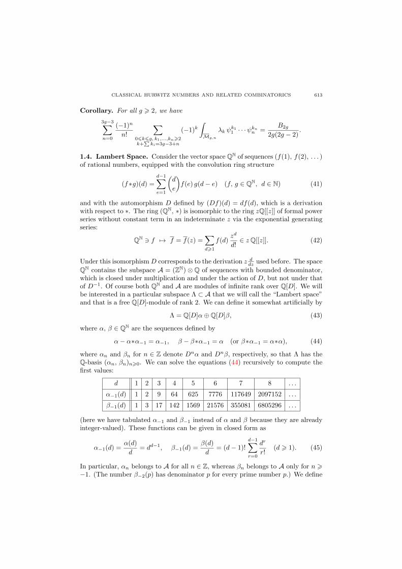
where αn and βn for n ∈ Z denote Dnα and Dnβ, respectively, so that Λ has theQ-basis (αn, βn)n>0. We can solve the equations (44) recursively to compute thefirst values:

d 1 2 3 4 5 6 7 8 . . .

α−1(d) 1 2 9 64 625 7776 117649 2097152 . . .

β−1(d) 1 3 17 142 1569 21576 355081 6805296 . . .

(here we have tabulated α−1 and β−1 instead of α and β because they are alreadyinteger-valued). These functions can be given in closed form as

α−1(d) =α(d)

d= dd−1, β−1(d) =

β(d)

d= (d− 1)!

d−1∑r=0

dr

r!(d > 1). (45)

In particular, αn belongs to A for all n ∈ Z, whereas βn belongs to A only for n >−1. (The number β−2(p) has denominator p for every prime number p.) We define


the extended Lambert space Λ+ by

Λ+ =

∞⊕n=−∞

Qαn ⊕∞⊕

n=−1

Qβn ⊂ A

and define two further subspaces of Λ+ by

Λ1 =

−1⊕n=−∞

Qαn, Λ2 =

∞⊕n=−∞

Qαn ⊕∞⊕n=0

Qβn,

so that Λ2 has codimension 1 in Λ+ and each of Λ, Λ+, and Λ2 is a Q[D]-module.

Proposition 2. Each of the spaces Λ, Λ1 and Λ2 is a ring with respect to themultiplication (41).

Proof. Set T = α−1 ∈ zQ[[z]], where α−1 is defined by (42). Then the first ofequations (44) says that (1 − T )D(T ) = T or 1

z dz = 1−TT dT , which integrates

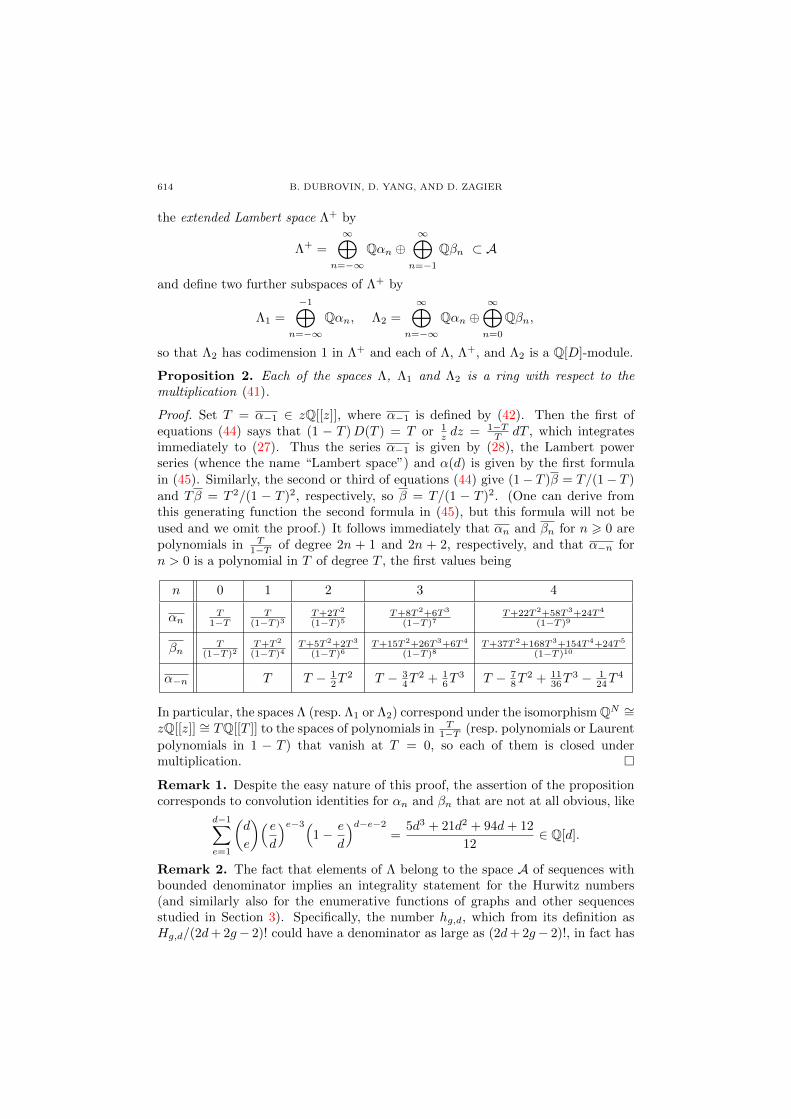
immediately to (27). Thus the series α−1 is given by (28), the Lambert powerseries (whence the name “Lambert space”) and α(d) is given by the first formulain (45). Similarly, the second or third of equations (44) give (1− T )β = T/(1− T )and Tβ = T 2/(1 − T )2, respectively, so β = T/(1 − T )2. (One can derive fromthis generating function the second formula in (45), but this formula will not beused and we omit the proof.) It follows immediately that αn and βn for n > 0 arepolynomials in T

1−T of degree 2n + 1 and 2n + 2, respectively, and that α−n forn > 0 is a polynomial in T of degree T , the first values being

n 0 1 2 3 4

αnT

1−TT

(1−T )3T+2T 2

(1−T )5T+8T 2+6T 3

(1−T )7T+22T 2+58T 3+24T 4

(1−T )9

βnT

(1−T )2T+T 2

(1−T )4T+5T 2+2T 3

(1−T )6T+15T 2+26T 3+6T 4

(1−T )8T+37T 2+168T 3+154T 4+24T 5

(1−T )10

α−n T T − 12T

2 T − 34T

2 + 16T

3 T − 78T

2 + 1136T

3 − 124T

4

In particular, the spaces Λ (resp. Λ1 or Λ2) correspond under the isomorphism QN ∼=zQ[[z]] ∼= TQ[[T ]] to the spaces of polynomials in T

1−T (resp. polynomials or Laurent

polynomials in 1 − T ) that vanish at T = 0, so each of them is closed undermultiplication.

Remark 1. Despite the easy nature of this proof, the assertion of the propositioncorresponds to convolution identities for αn and βn that are not at all obvious, like

d−1∑e=1

(d

e

)( ed

)e−3(1− e

d

)d−e−2

=5d3 + 21d2 + 94d+ 12

12∈ Q[d].

Remark 2. The fact that elements of Λ belong to the space A of sequences withbounded denominator implies an integrality statement for the Hurwitz numbers(and similarly also for the enumerative functions of graphs and other sequencesstudied in Section 3). Specifically, the number hg,d, which from its definition asHg,d/(2d+ 2g− 2)! could have a denominator as large as (2d+ 2g− 2)!, in fact has


denominator at most Ng d!, for some integer Ng depending only on g. On the otherhand, we do not know the combinatorial meaning of the divisibility of an elementof Λ by a power of (1−T )−1 (like the divisibility of Hg by (1−T )−2g+2), let alonethe meaning of the bottom coefficient.

We end this subsection with a few remarks on the asymptotics of sequences inthe Lambert space. The two basic sequences α and β have asymptotic growth givenby

α(d) ed

d!=

1√2πd

(1− 1

12d+

1

288d2+ · · ·

),

β(d) ed

d!=

1

2− 1√

2πd

(1

3+

1

540d− 25

6048d2+ · · ·

),

and the asymptotic growth of αn(d) and βn(d) for any n ∈ Z is obtained by mul-tiplying these by dn, so that we can give the asymptotics of any element f ∈ Λto arbitrary order in d−1/2. We can also see the same thing analytically usingthe isomorphism (42), by considering the behavior of f(z) as z → e−1. From theproposition and its proof we know that f(z) is a polynomial in 1/(1 − T ), so asε = 1−T tends to 0 (from above) we have f(z) ∼ Cε−D for some positive integer Dand non-zero rational number C. (These numbers D and C are what we called the“order of the most singular term” and the “top coefficient” in the discussion at theend of the introduction.) But from (27) we get 1−ez = 1−(1−ε)eε = 1

2ε2 +O(ε3),

so f(z) ∼ 2−D/2C(1 − ez)−D/2 as z tends to e−1 from below, and from this

and the binomial theorem one gets the asymptotics f(d)d! ∼

2−D/2CΓ(1+D/2) d

D/2−1ed or

f(d) ∼ 2−D/2C√

2πΓ(1+D/2) dd+(D−1)/2, as well as an expansion to higher orders if one wishes.

1.5. Asymptotics of the Hurwitz numbers. We end Section 1 with a discus-sion of the asymptotic behavior of the numbers Hg,d (or hg,d) for large values of gand d.

The large g asymptotics for Hg,d with fixed d > 2 follow immediately from thecorollary to Theorem 1 (Hurwitz’s theorem) and are given by (3). Notice thatthis asymptotic formula is extremely precise, since the error term is of the order

of(d−1

2

)2gand is hence exponentially smaller than the main term for g large. A

related comment is that the generating function Cd(x) for x ∈ R>0 fixed is alsogiven to high accuracy by the leading term approximation

Cd(x) ≈ 1

d!2exp((d

2

)x)

(d→∞). (46)

This is true, although not quite obvious, even for x small; e.g., for x = 0.1 theratio of the left- and right-hand sides of (46) differs from 1 by about 5 × 10−18

for d = 500 and 6×10−82 for d = 2000. In particular, the generating series H(x, y)defined in (1) is rapidly divergent for any positive values of x and y, so that it canonly be considered as a formal power series.

In the opposite direction for g fixed and d large, the discussion at the end of Sec-tion 1.4 together with the formula given in (35) for the “top coefficient” of the


element d 7→ d!hg,d of the Lambert space immediately imply the asymptotic state-ments (5) and (6). It is perhaps worth mentioning that one can also proceed in asomewhat different order, using the differential recursion (25) inductively to derivethe formula

Hg(z) ∼2−5(g−1)/224−gcg(5g − 1)(5g − 3)

(1− ez)−5(g−1)/2 for z → e−1

with cg satisfying (7) for the asymptotics of each function Hg(z) as z tends to e−1

from below and deducing the asymptotic formula for its Taylor coefficients fromthis. We suppress the details, since they are a little lengthy and basically justreproduce the arguments used in the proof of Theorem 3. Note that each individualterm of the expansion H(x, y) as

∑gHg(x2y)x2g−2 converges for |x2y| < 1/e, but

that the whole series does not converge for any positive values of x and y, asalready mentioned above. We can also see why this should be so from the “fixed g”asymptotics with g large. The numbers cg defined by (7) or (8) grow more thanexponentially, like

cg ∼√

3/5

π

(5√

2

eg)2g(1

g+

1

6g2+

1

72g3− 14459

810000g4+ · · ·

)as g →∞. (To see that this should be true up to a constant independent of g, onenotes that the recursion (7) has a formal solution C · 50g(g − 1)!2Pg for a uniquepower series Pg = 1− 49

3g3 + · · · . The rigorous proof that this formal solution gives

the correct asymptotics of cg, and the determination of the constant C =

√3/5

2π2 ,are given in various places in the literature [34], [33], [25], [45].) The renormalizedvalues occurring in (6) decay more than exponentially, like (e/720g)g/2, but this isnot enough to ensure convergence of the double series since together with (6) (as-suming that this estimate holds uniformly when g and d are both large, whichwe do not know) this would say that the (g, d) term of H looks roughly like(ed5x4/720g)g/2(ex2y)d and hence grows more than exponentially rapidly in therange when d goes to infinity more rapidly than g1/5. It remains an interestingopen question to find a uniform bound for hg,d or for Hg,d in terms of elementaryfunctions.

Remark. Another interesting question about enumerations of Hurwitz covers ofa torus has been systematically studied in [8], where the Lambert ring should bereplaced by the ring of quasi-modular forms. We hope to continue the study ofHurwitz covers of a Riemann surface of higher genus in future.

2. Computing Hg,d from the P1 Frobenius Manifold

In this section we describe a completely different approach, and a completelydifferent proof of the formula (34), using the Gromov–Witten (GW) invariants ofP1. Unlike the preceding section, this one is not elementary and we will assumefamiliarity with the theory of Frobenius manifolds.


The GW invariants of P1 are encoded by the generating series (“free energy”)

FP1

=∑g>0

FP1

g ε2g−2,

where the genus g part FP1

g is given by

FP1

g =∑n,d>0

1

n!

∑p1,...,pn>0

16α1,...,αn62

tα1p1 . . . t

αnpn

∫[Mg,n(P1,d)]virt

ev∗1(φα1) · · · ev∗n(φαn)ψp11 · · ·ψpnn .

Here t1p, t2p (p > 0) are indeterminates, φ1 = 1 and φ2 = ω are the standard basis

of H∗(P1) (with ω normalized by∫P1 ω = 1), Mg,n(P1, d) is the moduli space of

stable maps of degree d of curves of genus g with n marked points to the targetP1, evi denotes the i-th evaluation map and ψi the first Chern class of the i-thtautological line bundle onMg,n(P1, d). It was proved by Pandharipande [43] thatthe Hurwitz numbers Hg,d coincide with the following special GW invariants of P1

Hg,d =

∫[Mg,n(P1,d)]virt

ev∗1(ω) · · · ev∗n(ω)ψ1 · · ·ψn,

where n is defined as 2g + 2d − 2 (the integral vanishes for other values of n), so

FP1

g is related to the generating series Hg of Section 1 by

t2g−2Hg(t2) = FP1

g

∣∣t21=t, tαp=0 otherwise

, (47)

where the variable t2 corresponds to the variable z = x2y of Section 1.3 and the full

generating series FP1

coincides with our H(x, y) under the substitution t =√z,

ε = x/√z = 1/y.

We now apply the DZ approach to calculating these special GW invariants. Eventhough only the specialization tαp = δp1δα2t of the variables tαp is used in (47), wehave to work with the 2-variable specialization with a second non-zero variablet10 = s, and will only restrict to s = 0 at the end. The potential of the P1 Frobeniusmanifold is given by

F =u v2

2+ eu,

where u, v are the flat coordinates (∂v gives the unit vector field), which in turnwill be expressed as power series in t and s. The power series (u, v) is the so-calledtopological solution, obtained by solving the following genus zero Euler–Lagrangeequation (see details in [9], [18]):

∂Φ

∂u=∂Φ

∂v= 0, where Φ = s u+ t

∂F

∂u− u v = s u+ t

(v2

2+ eu

)− u v.

This has a unique solution u(s, t), v(s, t) ∈ C[[s, t]] satisfying u(s, 0) = 0, v(s, 0) =s, given by

u = s t+ T, v = s+ T/t with T defined by t2 est = T e−T . (48)


The first several terms of the expansions of u, v near s = 0, t = 0 read

u = s t+ t2 + s t3 +s+ 2

2t4 +

s3 + 12s

6t5 +

s4 + 48s2 + 36

24t6 + · · · ,

v = s+ t+ s t2 +s2 + 2

2t3 +

s3 + 12s

6t4 +

s4 + 48s2 + 36

24t5 + · · · .

Let us now compute FP1

g . Begin with g = 0. By [9], [19], we have

FP1

0 =s2

2Ω1,0;1,0 − sΩ1,0;1,1 + s tΩ1,0;2,1 +

1

2Ω1,1;1,1 − tΩ1,1;2,1 +

t2

2Ω2,1;2,1,

where Ωα,p;β,q are the genus 0 two-point functions. Substituting the known explicitexpressions

Ω1,1;1,1 = (2− 2u+ u2)eu + u v2, Ω1,1;2,1 = u v eu +v3

3, Ω2,1;2,1 =

e2u

2+ v2 eu

into this formula and specializing to s = 0, we find

FP1

0

∣∣s=0

=2T 3 − 9T 2 + 12T

12 t2,

which in view of (47) agrees with our previous formula (30) (with Te−T = t2 = z).

We next consider g = 1. The generating function FP1

g in this case has the form

FP1

1 =1

24log(v2s − w u2

s

)− u

24.

Substituting the solution (48) into this formula and using (47) we obtain

H1(z) =1

24log

1

1− T− T

24,

again in agreement with our previous formula (32).The expression for the genus two part of the free energy is more involved [18], [11]:

5760FP1

2 = −w2

∆4

[512u3

svsv3ss + 384wu3

svss(u2s + 2uss)(u

2svs + 2ussvs− 2usvss)

− 64w2u4s(u

2s + 2uss)

3]

− w

∆3

[256usvsv

3ss + 12wus(28u4

svsvss + 116u2sussvsvss + 64u2

ssvsvss

+ 28usvsusssvss− 69u3sv

2ss− 128usussv

2ss + 14u3

svsvsss + 28usvsussvsss

− 28u2svssvsss)−w2u2

s(u2s + 2uss)(121u4

s + 538u2suss + 256u2

ss + 168ususss)]

+w

∆2

[−2(42u3

svsvss + 126usussvsvss + 42usssvsvss− 95u2sv

2ss− 96ussv

2ss

+ 30u2svsvsss + 42ussvsvsss− 126usvssvsss + 20usvsvssss)

+w(72u6s + 479u4

suss + 626u2su

2ss + 64u3

ss

+ 224u3susss + 252usussusss + 40u2

sussss)]

+1

∆

[22v2

ss− 24vsvsss +w(17u4s + 102u2

suss + 56u2ss + 68ususss + 20ussss)

]+ 7uss,

(49)


where ∆ = v2s−w u2

s. Using the expressions (48) for u, v we find that ∆|s=0 = 11−T ,

so we obtain

H2(z) =1

1440

T 2(1 + 6T )

(1− T )5,

in agreement with the first formula in (33).To proceed to higher genera, one can solve, recursively in g, the loop equation [18],

[19]. Noting that

v(0, t) =T

t, u(0, t) = T, vs(0, t) =

1

1− T, us(0, t) =

t

1− T,

∂`v

∂s`(0, t) = t`−1D`(T ),

∂`u

∂s`(0, z)(0, z) = t`D`(T ) (` > 2),

we find by the (3g − 3)-Lemma [18] that the function Hg has the form (34) forall values of g (Goulden–Jackson–Vakil theorem). As the above solution for g = 2makes clear, it would not be easy to calculate Hg explicitly this way for large values

of g. On the other hand, it should be emphasized that the formulas FP1

g obtainedby this approach, such as the formula (49) for the case g = 2, would hold withoutany modification for the general GW invariants (i.e., without the specialization totαp = 0 for (p, α) 6= (1, 2)), with only the form of Φ changing. It is worth notingthat the DZ loop equation for solving FP1

g is quadratic, and also universal in allsemisimple homogeneous cohomological field theories, with the same form in allcases and the dependence on the Frobenius manifold arising only through its Eulervector field and periods.

3. Connection to Various Models in Enumerative Geometry

In this section we will look in detail at three other problems whose solutionsbelong to the Lambert space defined in Section 1.4: the enumerations of ordinarygraphs and of ribbon graphs, and the computation of certain Hodge integrals thatinclude the Hurwitz numbers as a special case. The discussion of the first case iselementary and self-contained, but the discussion of the two other cases assumessome familiarity with moduli space theory.

3.1. Enumeration of graphs. In this subsection we discuss the enumeration ofgraphs. Denote by Gg,d the number of connected graphs with d vertices and gindependent loops (i.e., first Betti number g), where graphs are allowed to havemultiple (non-oriented) edges and by “number” we mean the weighted number inwhich each graph Γ is counted with multiplicity 1/|Aut(Γ)|, the reciprocal of itsnumber of symmetries. For instance, G1,2 = 3

4 because there are two graphs withtwo vertices and one loop, a “tadpole” with a symmetry group of order 2 (reflectthe loop) and a 2-gon with symmetry group of order 4 (interchange the two verticesor the two edges), and Gg,1 = 1/2gg! for all g because the only 1-vertex graph withg loops is a bouquet of g circles that can be arbitrarily re-oriented or permuted. Inthis subsection we describe the numbers Gg,d when either d or g is fixed, finding inboth cases results exactly analogous to those for the numbers hg,d. Most or all of


these results are certainly known (see for example [46]), but we give a presentationthat is as close as possible to the one for the Hurwitz case.

We begin with a discussion of the case of fixed d.

Theorem 4. For each d > 1, the generating series

Bd(x) =∑g>0

Gg,d xg+d−1

of graphs with d vertices is a polynomial of degree d2 in ex/2 of the form

Bd(x) =1

d!

∑d6m6d2

m≡d (mod 2)

cd,m emx/2, (50)

where the coefficients cd,m are integers with cd,d2 = 1, cd,m = 0 for d2 − 2d + 2 <

m < d2, and cd,d = (−1)d−1(d− 1)!. These polynomials are determined completelyeither by the linear recursion

Bd(x) =ed

2x/2

d!− 1

d

d−1∑k=1

d− kk!

ek2x/2Bd−k(x) (51)

or by the quadratic recursion

Bd(x) =1

d2 − d

d−1∑k=1

k (d− k) (ekx − 1)Bk(x)Bd−k(x) (d > 2) (52)

or by the quadratic differential recursion(2d

dx− d2

)Bd(x) =

d−1∑k=1

k (d− k)Bk(x)Bd−k(x). (53)

Corollary. The numbers Gg,d for fixed d have the form

Gg,d =1

d! (d+ g − 1)!

∑16m6d2

m≡d (mod 2)

cd,m (m/2)g+d−1

with cd,m as above, the first values being given by

d 2ww! d!Gg,d, where w = g + d− 1

1 1

2 4w − 2w

3 9w − 3 · 5w + 2 · 3w

4 16w − 4 · 10w − 3 · 8w + 12 · 6w − 6 · 4w

5 25w − 5 · 17w − 10 · 13w + 20 · 11w + 30 · 9w − 60 · 7w + 24 · 5w


Proof. The proof follows the same idea as the second approach to Theorem 1 in Sec-tion 1.2, via disconnected Hurwitz numbers. For k, d > 0 let Nk,d denote thenumber of graphs (not necessarily connected) with d vertices and k edges, where“number” has the same meaning as for Gg,d above, and let

ZG = ZG(x, y) =∑

Γ

xe(Γ)yv(Γ)

|Aut(Γ)|=∑k, d>0

Nk,d xk yd (54)

(where e(Γ) and v(Γ) denote the number of edges and number of vertices of agraph G) be the corresponding generating series, called the partition function ofgraph counting. By the usual principle that the generating series for all objectsof a given type is the exponential of the generating series for the connected ones,together with the observation that a connected graph with d vertices and g loopshas Euler number 1− g and hence has g + d− 1 edges, we have

ZG = ZG(x, y) = eG(x,y), (55)

where

G(x, y) =∑

Γ connected

xe(Γ)yv(Γ)

|Aut(Γ)|=

∑g>0, d>1

Gg,d xg+d−1 yd =

∞∑d=1

Bd(x) yd (56)

is the two-variable generating series for connected graphs. On the other hand,it is easy to see that Nk,d = d2k/2kk! d!, since there are 2kk! d! ways to numberand orient the edges and number the vertices (after which there are no longer anyautomorphism) and then d2k ways to map the 2k numbered endpoints of the edgesto the d numbered vertices. This gives the closed formula

ZG(x, y) =∑d>0

yd

d!ed

2x/2 . (57)

for the partition function ZG . Formulas (55)–(57) already imply that the coefficientsBd(x) of G(x, y) belong to Q[ex/2] and have the form given in (50). Formula (57)also implies the differential equations

DZG(x, y) = y ex/2 ZG(x, yex), D2ZG(x, y) = 2∂ZG(x, y)

∂x(58)

for ZG , where D = y ∂∂y , and these and (55) give the differential equations

D(ZG) = D(G)ZG , (59)

(D2 −D)G(x, y) = DG(x, y)(DG(x, yex)−DG(x, y)

), (60)

(DG)2 +D2G = 2∂G∂x

(61)

for G, which in turn are equivalent to the three recursions (51)– (53).

We now turn to the opposite case, when g is fixed.

Theorem 5. The generating series

Gg(z) =

∞∑d=1

Gg,d zd (62)


belongs to the extended Lambert space for all g. It is given for g 6 2 by

G0(z) = T − T 2

2, G1(z) =

1

2log

1

1− T, G2(z) =

3T + 2T 2

24(1− T )3(63)

(where z = T e−T as usual) and in general by an expression of the form

Gg =

3g−3∑i=g−1

λg,i(1− T )i

(64)

for all g > 2, with top and bottom coefficients given by

λg,g−1 =Bg

g (g − 1), λg,3g−3 = bg−1, (65)

where Bn denotes the nth Bernoulli number and the numbers br are defined by thegenerating series

∞∑r=1

br xr = log

( ∞∑m=0

(6m)!

(3m)! (2m)!

( x

288

)m)

=5

24x+

5

16x2 +

1105

1152x3 +

565

128x4 +

82825

3072x5 + · · · . (66)

Proof. We will outline three proofs. We first give a “pure thought” proof of thestatements that Gg is given by (63) for g 6 1 and is a polynomial in 1/(1 − T ) ofdegree 3g − 3 and leading coefficient bg−1 for all g > 2. We then sketch two otherproofs of these statements, and also of the formula for the “bottom” coefficientin (65), based on the closed formula (57) for eG .

Consider first the case g = 0. The number G0,d counts trees (connected andsimply connected graphs) on d vertices. The number dG0,d counts rooted trees(trees with one marked vertex, the “root”), because there are d ways to choose theroot of a given tree and the factors 1/|Aut(Γ)| in the definitions of G0,d and G1,d

ensure that everything works correctly. Denote by T (z) = DG0(z) =∑d>1 dG0,dz

d

the generating series of rooted trees. Then the generating series of rooted trees inwhich the root has valency k is clearly zT (z)k/k!, with the factor z correspondingto the root and the factor T (z)k/k! to the fact that the complement of the rootis the union of k rooted trees (the root being the other end of one of the edgesgoing to the original root). Since the root of every tree has some valency, we getT (z) =

∑∞k=0 zT (z)k/k! = zeT (z), and hence T (z) is indeed equal to the series

defined by (27). This proves the case g = 0 of (63), and the Lagrange inversionformula (28) gives the explicit formula d!G0,d = dd−2, which is Cayley’s famousresult for the number of trees on d given vertices.

Next consider g = 1. A graph with Betti number 1 has a unique cycle (withno backtracking). If this cycle contains k vertices, then the graph is the unionof the cycle and k rooted trees, the roots being the vertices on the cycle, so thecontribution to G1(z) coming from all such graphs is T (z)k/2k, with the factor 2kcorresponding to the automorphisms of the cycle (rotations and reflection). Thisgives G1(z) =

∑∞k=1 T (z)k/2k and hence proves (63) for g = 1.


Now suppose that g > 2. There is a map from the set Grg of graphs with g loops

to the set Gr>3g of graphs with g loops and having only vertices of valency > 3: if

a graph has a 1-valent vertices, we remove this vertex and the corresponding edgeand keep doing this until there are no 1-valent vertices left, and if the graph thenhas any 2-valent vertices, we remove them and fuse the corresponding two edgesinto a single new one. This map is clearly surjective, with the graphs that map toa given (> 3)-valent graph Γ being given by attaching a rooted tree to any vertexof Γ, which gets identified with the root of the tree, and any number n > 0 ofrooted trees to any edge of Γ, where the roots become new internal points on thatedge. Thus the contribution to the generating function Gg(z) of each vertex of Γis T (z), and the contribution of each edge is

∑∞n=0 T (z)n = 1/(1 − T (z)), giving

the identity

Gg(Te−T ) =∑

Γ∈Gr>3g

1

|Aut(Γ)|T v(Γ)

(1− T )e(Γ)=

∞∑n=1

G(>3)g,n

Tn

(1− T )g+n−1, (67)

where G(>3)g,n is the weighted number of connected (> 3)-valent graphs with n ver-

tices and g loops. On the other hand if such a graph Γ has ni vertices of va-lency i, then n and k = e(Γ) = n + g − 1 are given by n = n3 + n4 + · · · and2k = 3n3 + 4n4 + · · · , respectively, so n3 + 2n4 + · · · = 2g − 2 and in particularn 6 2g − 2. This shows that Gg(z) for g > 2 is a polynomial of degree 3g − 3in 1/(1−T ) with top coefficient equal to the number of connected trivalent graphswith first Betti number g. But this number is clearly equal to bg−1 with br givenby (66), since the weighted number of not-necessarily-connected trivalent graphswith d vertices and k edges is clearly non-zero only if d = 2m and k = 3m for

some m and is then equal to (6m)!288m(3m)! (2m)! . (Start with a set of 3m labelled and

oriented edges and 2m labelled Y -shaped vertices; then there are (6m)! ways toidentify the 6m half-edges of the two sets and we must divide by the 23m(3m)!ways to renumber and re-orient the edges and the 3!2m(2m)! ways to renumberand relabel the vertices.) This concludes the proof of Theorem 5, except for thestatement about the lowest-order term in (64).

Note the similarity of (67) to (40), with a power series in z becoming a polynomialin (1− T )−1 by the same mechanism in both cases: in the ELSV case, the originalsum (39) permitted all values ki > 0 and was infinite, while the new sum (40) haski > 2 and hence is finite because

∑(i − 1)ki = 3g − 3 − k is fixed, while in the

graph case the original generating function Gg(z) includes all valencies r > 1 butthe sum in (67) has valencies r > 3 and hence is bounded because

∑(r − 2)nr =

2g−2. In both cases the reduction is achieved using the so-called string and dilatonequations [32], [28], [46], [44], [13], [15] that arise in these models.

We now briefly indicate the two alternative proofs mentioned above of the state-ment that the function d 7→ d!Gg,d belongs to the (extended) Lambert spacefor g > 0. The first is exactly similar to the proof of the corresponding state-ment for the Hurwitz numbers given in Section 1.3. We substitute the expansion

G(x, y) =

∞∑g=0

Gg(xy)xg−1


into the recursive functional equation (60) for G to get the recursive differentialequation

G(2)g − G(1)

g =∑

g1,g2>0, `>1g1+g2+`=g+1

1

`!G(1)g1 G

(`+1)g2 (68)

for the generating series Gg, and then argue exactly as in the proof of Theorem 3 toget all of the assertions of Theorem 5, including the statement about the “bottom”coefficients that was not included in our first proof. We omit the details. Aboutthe bottom coefficients we remark only that it is surprising that the formula is sosimilar to the one in the Hurwitz case (except for the doubling of the index). Aboutthe top coefficients, it follows from (68) that the second of equations (65) holds withbr defined inductively by

b1 = 1, br = 6 r br−1 + 5∑

r1+r2=r−1

br1 br2 for r > 2, (69)

where br = 6r5 4rbr (which is an integer by virtue of this recursion). This in fact

coincides with the generating function definition (66) of the br, because by loga-rithmically differentiating (66) and using the linear differential equation satisfied

by the hypergeometric function∑ (6m)!

(2m)!(3m)! tm one obtains the Riccati equation

dV

dX− 1

2V 2 +

1

2X = 0,

for the generating function V = −X1/2 + 12X−1 + 3

∑r>1 rbrX

−1−3r/2, and this

in turn is equivalent to the recursion (69). We also mention that, as well as theircombinatorial interpretation in terms of counting trivalent graphs, the numbers broccur in the Faber–Zagier formulas [22] for the first relation in the tautologicalsubring of the cohomology ring (or Chow ring) of the moduli spaces of curves;see also for example [2], [44], [5] for some related questions where the numbers brappear.

Finally, we can prove Theorem 5 directly from (55) and (57) by an argumentusing Gaussian integrals, and we sketch this method briefly also since it is simpleand works in many situations. Substituting the identity

en2x/2 =

1√2πx

∫ ∞−∞

exp(nu− u2/2x) du

into (57), we get

ZG(x, z/x) =1√2πx

∫ ∞−∞

exp(zeu − u2/2

x

)du.

Consider the expansion of this for x small by the method of stationary phase. Theargument of the exponential takes on its maximum when its derivative (zeu−u)/xvanishes, so at u = T , where T is defined by (27). Expanding around this point,


we find

ZG(x, z/x) =1√2πx

∫ ∞−∞

exp(zeT+v − (T + v)2/2

x

)dv

=1√2πx

exp(T − T 2/2

x

) ∫ ∞−∞

exp(−1− T

2xv2 +

∞∑r=3

T

r!xvr)dv

= exp

(T − T 2/2

x+

1

2log

1

1− T

)1√2π

∫ ∞−∞

e−w2/2

(1 +

Tw3

6(1− T )3/2

√x

+

(T 2w6

72(1− T )3+

Tw4

24(1− T )2

)x+ · · ·

)dw

= exp

(T − T 2/2

x+

1

2log

1

1− T+

(5T 2

24(1− T )3+

T

8(1− T )2

)x+ · · ·

),

where in the last two lines we have substituted v =(

x1−T

)1/2w and used that

12π

∫∞−∞ e−w

2/2 wn dw equals (n− 1)!! for n even and 0 for n odd. This shows that

logZG(x, z/x) has the form∑g>0 Gg(z)xg−1 with G0, G1 and G2 as in (63) and,

by expanding further, that the general coefficient Gg(x) is always a polynomial in1/(1 − T ). One also sees that this polynomial has degree 3g − 3 and top coef-ficient bg−1 as defined by (66), since the highest power of 1/(1 − T ) for a givenpower of x comes from exponentiating the first term Tv3/6x of the argument of theexponential function.

The following corollary follows immediately by Theorem 5 and by the generalremarks made in Section 1.4 about the asymptotics of sequences belonging to theLambert space.

Corollary. The asymptotic growth of the numbers Gg,d for fixed g > 0 is given by

Gg,d ∼5 bg−1

2(7g−3)/2 Γ( 3g−12 )

d(3g−5)/2 ed (d→∞), (70)

where br = 6r5 4rbr are the integers defined by (69) for r > 1 and b−1 = − 1

10 ,

b0 = 15 .

Before ending this subsection, we mention that the interesting relationship be-tween enumeration of graphs and Hurwitz numbers discussed here should be re-vealed in other, more subtle ways. For example, Cayley’s famous formula can beproved by counting the multiplicity of the quasi-homogeneous Lyashko–Looijengamapping assigning to a polynomial of degree d with d − 1 critical values. For thisinteresting direction, we omit the details but only refer to Arnold’s paper [1] andthe references therein. We hope to return to this question in the future.

3.2. Ribbon graphs. We now turn to our second model, related to the counting ofribbon graphs with even valencies. Here the corresponding generating function F—called the “GUE (Gaussian unitary ensemble) free energy of even couplings” be-cause of its alternative method of calculation using matrix integrals — and its genus


g parts Fg are defined by

F = F(X, s; ε)

=X2

2ε2

(logX − 3

2

)− 1

12logX + ζ ′(−1) +

∑g>2

ε2g−2 B2g

4g(g − 1)X2g−2

+∑g>0

ε2g−2∑n>0

∑j1,...,jn>1

(∑Γ

1

# Aut(Γ)

)sj1 . . . sjn X

2−2g−(n−|j|),

=:

∞∑g=0

ε2g−2Fg(X, s), (71)

where the internal sum is taken over all connected oriented ribbon graphs of genusg with labelled half-edges and with unlabelled vertices of valencies 2j1, . . . , 2jn,Aut(Γ) denotes the symmetry group of Γ, and |j| := j1 + · · ·+ jn. Actually, the fullGUE free energy computes the numbers of ribbon graphs with arbitrary valencies,but here we can treat only the case when all valencies are even. Also, we willactually consider a specialization of (71), which seems to be new. The possibilityof effective computation of the new model is due to the recently discovered Hodge–GUE correspondence [17], [14].

It will be convenient to renormalize the couplings by setting sk =(

2kk

)sk. We

define w = w(X, s) as the unique series solution in s to the following equation

w = X +∑k>1

k sk wk, w(X, s) = X + · · · . (72)

The following theorem was recently obtained in [17].

Theorem [17]. The genus zero part of GUE free energy with even couplings hasthe expression

F0 =w2

4−X w +

∑k>1

sk

(X wk − k

k + 1wk+1

)+

1

2

∑k1,k2>1

k1k2

k1 + k2sk1 sk2w

k1+k2 +X2

2logw. (73)

For g > 1, there exist functions Fg(z0, z1, . . . , z3g−2), g > 1 of independent vari-ables z0, z1, z2, . . . , z3g−2 such that

Fg(X, s) = Fg

(u(X, s),

∂u(X, s)

∂X, . . . ,

∂3g−2u(X, s)

∂X3g−2

), g > 1. (74)

Here

u(X, s) :=∂2F0(X, s)

∂X2= logw(X, s).

We now specialize the sk to

sk =s

k · k!(k > 1), (75)


where s is a parameter. (At the end of the argument we will further specializeto X = s − 1. One can also consider the more general specialization X = s + a,where a is an arbitrary nonzero parameter, in which case Fg has two singularitiesin the complex z-plane. This case will be treated in a subsequent publication.)Substituting (75) into equation (72) gives the equation

w = X + s (ew − 1)

for the power series w = w(X, s). We can rewrite this as w = X−es/e+T(seX−s

),

where T (z) is the Lambert series (28). It follows immediately that the functionu(X, s) = logw(X, s) and its X-derivatives specialize under s = ez, X = s− 1 to

u(ez − 1, ez) = log(T − 1),∂mu

∂Xm(ez − 1, ez) =

Qm(T )

(1− T )2m(m > 1), (76)

where z = Te−T as usual and where Qm(T ) is a polynomial of degree m − 1 in Twith integer coefficients, with Q1 = −1. Then we have

F = F(ε, z) := F(X, s; ε)∣∣sk=

e zk·k! , X=e z−1

=(ez − 1)2

2ε2

(log(ez − 1)− 3

2

)− 1

12log(ez − 1) + ζ ′(−1)

+∑g>2

ε2g−2 B2g

4g(g − 1)(ez − 1)2g−2

+∑

Γ

ε2g(Γ)−2 (ez)|V (Γ)|

# Sym Γ(ez − 1)|F (Γ)|

|V (Γ)|∏i=1

1vali(Γ)

2 ·(vali(Γ)

2

)!

(77)

=:∑g>0

ε2g−2Fg(z).

Here the last summation in (77) is taken over all connected oriented ribbon graphsΓ with labelled half-edges and unlabelled vertices of even valencies, V (Γ) denotesthe set of vertices of Γ, val1(Γ), . . . , val|V (Γ)|(Γ) the valencies, E(Γ) the set of edges,F (Γ) the set of faces, and g(Γ) the genus.

Theorem 6. For g = 0, 1, 2, 3, Fg(z) have the following explicit expressions

F0(z) =T 2

4− T

2− 3

4+

1

2log(T − 1)−

(Γ(0, 2− 2T ) + γ + iπ + log 2

) T 2

2e2−2T

+(Γ(0, 1− T ) + 1 + γ + iπ

)T e1−T ,

F1(z) =1

12log(−1) + ζ ′(−1) +

1

12log

1

(1− T )2,

F2(z) = −8T 3 + 43T 2 + 26T + 12

2880 (1− T )4,

F3(z) =32T 6 + 7392T 5 + 19953T 4 + 3668T 3 − 538T 2 + 1868T + 720

725760 (1− T )8,

where γ denotes Euler’s constant, Γ(0, x) denotes the incomplete Gamma function,and z = Te−T . Moreover, ∀ g > 2, Fg(z) belongs to the Lambert space, more


precisely,

Fg(z) =

4g−4∑i=g−1

µg,i(1− T )i

, (78)

where µg,i are rational numbers satisfying∑4g−4i=g−1 µg,i =

B2g

2g(2g−2) .

Proof. The validity of (78) is ensured by equations (74) and (76) together with the

vanishing of∂Fg∂z0

for g > 2 and homogeneity statements for Fg that can be proved by

using the Hodge–GUE correspondence [17], [14]. To obtain the explicit expressionsof F2 and F3, one can use the formulas of F2, F3 in [17] with the specialization (76).So far, we do not know formulas for the top and the bottom coefficients µg,4g−4

and µg,g−1 for general values of g.

3.3. Hodge integrals. In this final section we consider the evaluation of certainintegrals over moduli spaces of curves that turn out to give a huge class of furthersequences belonging to the Lambert space, and generalizing the original Hurwitznumbers studied in Section 1.

Let Mg,n denote the Deligne–Mumford moduli space of stable algebraic curvesof genus g with n distinct marked points. Denote by Li the i-th tautological linebundle on Mg,n, by E the rank g Hodge bundle, and by ψi the first Chern classc1(Li), i = 1, . . . , n. We define the Hodge free energy as the generating series

HHodge = HHodge(t; x; ε) =∑g>0

HHodgeg (t; x) ε2g−2

of genus g parts defined by

HHodgeg (t; x) =

∑n>0

∑i1,...,in>0

ti1 · · · tinn!

∫Mg,n

exp(∑j>0

x2j−1 ch2j−1(E))ψi11 · · ·ψinn .

Here t0, t1, t2, . . . are indeterminates (“coupling constants”), x1, x3, . . . are pa-rameters, t = (t0, t1, . . . ), and x = (x1, x3, . . . ). According to Mumford [39],the even components of the Chern character of E vanish. Hence HHodge gives thegenerating series of Hodge integrals of the most general type.

We now define v = v(t0, t1, t2, . . . ) as the unique power series solution to∑i>0

tii!vi = v . (79)

By the Lagrange inversion formula, v has the following explicit expansion

v =∑k>1

1

k

∑p1+···+pk=k−1

tp1p1!· · · tpk

pk!.

We also set vm = ∂mt0 v for all m > 0. The following theorem for HHodgeg was proved

in [13].


Theorem [13], [15]. We have

HHodge0 (t; x) =

v3

6−∑i>0

tivi+2

i! (i+ 2)+

1

2

∑i,j>0

titjvi+j+1

(i+ j + 1) i! j!,

HHodge1 (t; x) =

1

24log v1 +

x1

24v.

For g > 2, there exist algorithmically computable functions HHodgeg (z1, . . . , z3g−3;

x1, x3, . . . , x2g−1), rational in z1 and polynomial in all the other variables, suchthat

HHodgeg (t; x) = HHodge

g (v1, . . . , v3g−3; x1, x3, . . . , x2g−1). (80)

Moreover, the functions HHodgeg satisfy the homogeneity conditions

3g−3∑m=1

mzm∂HHodge

g

∂zm= (2g − 2)HHodge

g , (81)

3g−3∑m=2

(m− 1) zm∂HHodge

g

∂zm+

g∑j=1

(2j − 1)xj∂HHodge

g

∂xj= (3g − 3)HHodge

g . (82)

We will be interested in the specialization of HHodgeg when all variables ti have

the same value z, in which case we write simply z for t. For this value of t we have

HHodge(z; x; ε) =∑g,n>0

cg,n(x) ε2g−2 zn, HHodgeg (z; x) =

∑n>0

cg,n(x) zn

with

cg,n(x) :=1

n!

∑i1,...,in>0

∫Mg,n

exp(∑j>0

x2j−1 ch2j−1(E))ψi11 · · ·ψinn .

To compute HHodgeg (z; x), we first make the smaller specialization when ti = t1

for i > 1 but t0 is still an independent variable, and will then specialize to t0 = t1 =z at the end. (Compare Section 2, where we kept only two variables s and t of theinfinitely many variables tαp and specialized to s = 0 at the end.) Then equation(79) simplifies to

t0 + t1 (ev − 1) = v.

This means that if we set t1et0−t1 = Te−T , then v = v(t0, t1, t1, . . . ) is given by

v = t0 − t1 + T . It follows easily that vm(z) = vm(z, z, . . . ) is given by

vm(z) = DmT (z) + δm,1 = αm−1 + δm,1 (m > 0), (83)

where D = z ddz as usual and αm−1 is defined in Section 1.4. This means a very

simple explicit formula for vm(z): the coefficient of zd in vm(z) is dd+m−1 forall d > 1.

Theorem 7. The power series HHodgeg (z; x)+δg,0(z+z2/4) belongs to the extended

Lambert space for every g > 0 and every x = (x1, . . . , x2g−1). These power series


are given explicitly for g = 0, 1, 2 by

HHodge0 (z; x) +

z2

4+ z =

T 3

6− 3T 2

4+ T, (84)

HHodge1 (z; x) =

1

24log

1

1− T+T

24x1, (85)

HHodge2 (z; x) =

2x31 − 42x2

1 + 78x1 − x3 − 24

34560 (T − 1)2+−7x2

1 + 38x1 − 31

5760 (T − 1)3

+5x1 − 11

1152 (T − 1)4− 7

1440 (T − 1)5. (86)

In general, for g > 2, HHodgeg (z; x) has the form

HHodgeg (z; x) =

5g−5∑i=2g−2

`g,i(x)

(1− T )i, g > 2, (87)

where `g(x) are polynomials in x1, x3, . . . , x2g−1. Moreover, `g,5g−5(x) is inde-pendent of x and is equal to 24−gcg/((5g − 3)(5g − 5)), where cg is defined by (7)or (8).

Proof. The formulas (84)–(86) can be obtained from the algorithm developed in [13]with the particular vm given by (83). The formula (87) follows from (80), (83) andthe homogeneity conditions (81), (82). The fact that `g,5g−5 does not depend on xis due to the dimension-degree matching.

We note that the first statement of Theorem 7 is a particular case of the Theo-rem 1 in [46], but no algorithm is given there to compute the Hodge integrals.

Noting that

1− λ1 + λ2 − · · ·+ (−1)gλg = exp

(−∑j>1

(2j − 2)! ch2j−1

)we have from the ELSV formula (39) that

Hg(z) :=∑d>0

hg,d zd = HHodge

g (z; −0!, −2!, −4!, . . . , −(2g − 2)!).

Thus the generating series Hg(z; x) generalizes the power series Hg(z) of Section 1,and Theorem 7 generalizes Theorem 3. (For instance, for g = 2 we verify easilythat under x1 = −1, x3 = −2, the formula (86) becomes (33).) Combining the twotheorems, we obtain

Corollary. For any fixed g > 0, and any fixed value x = (x1, . . . , x2g−1), thefunction HHodge

g (z; x) is analytic around z = 0, and has the dominant singularity

at z = e−1. As n→∞cg,n(x) ∼ hg,n.


References

[1] V. I. Arnold, Topological classification of complex trigonometric polynomials and the com-

binatorics of graphs with an identical number of vertices and edges, Funktsional. Anal. i

Prilozhen. 30 (1996), no. 1, 1–17, 96 (Russian). MR 1387484. English translation: Funct.Anal. Appl. 30 (1996), no. 1, 1–14.

[2] M. Bertola, B. Dubrovin, and D. Yang, Correlation functions of the KdV hierarchy and

applications to intersection numbers over Mg,n, Phys. D 327 (2016), 30–57. MR 3505204

[3] D. Bessis, C. Itzykson, and J. B. Zuber, Quantum field theory techniques in graphical enu-meration, Adv. in Appl. Math. 1 (1980), no. 2, 109–157. MR 603127

[4] V. Bouchard and M. Marino, Hurwitz numbers, matrix models and enumerative geometry,

Proc. Sympos. Pure Math., vol. 78, Amer. Math. Soc., Providence, RI, 2008, pp. 263–283.MR 2483754

[5] A. Buryak, F. Janda, and R. Pandharipande, The hypergeometric functions of the Faber–

Zagier and Pixton relations, preprint arXiv:1502.05150 [math.AG].[6] N. Caporaso, L. Griguolo, M. Marino, S. Pasquetti, and D. Seminara, Phase transitions,

double-scaling limit, and topological strings, Phys. Rev. D 75 (2007), no. 4, 046004, 24.

MR 2304432[7] G. Carlet, B. Dubrovin, and Y. Zhang, The extended Toda hierarchy, Mosc. Math. J. 4

(2004), no. 2, 313–332, 534. MR 2108440

[8] D. Chen, M. Moeller, and Z. Don, Quasimodularity and large genus limits of Siegel–Veechconstants, preprint arXiv:1606.04065 [math.NT].

[9] B. Dubrovin, Geometry of 2D topological field theories, Integrable systems and quantumgroups (Montecatini Terme, 1993), Lecture Notes in Math., vol. 1620, Springer, Berlin, 1996,

pp. 120–348. MR 1397274

[10] B. Dubrovin, Hamiltonian perturbations of hyperbolic PDEs: from classification results tothe properties of solutions, New trends in mathematical physics. Selected contributions of the

XVth international congress on mathematical physics (V. Sidoravicius, Ed.), Springer, 2009,

pp. 231–276.[11] B. Dubrovin, Gromov–Witten invariants and integrable hierarchies of topological type, Topol-

ogy, geometry, integrable systems, and mathematical physics, Amer. Math. Soc. Transl. Ser.

2, vol. 234, Amer. Math. Soc., Providence, RI, 2014, pp. 141–171. MR 3307147[12] B. Dubrovin, Symplectic field theory of a disk, quantum integrable systems, and Schur poly-

nomials, Ann. Henri Poincare 17 (2016), no. 7, 1595–1613. MR 3510464

[13] B. Dubrovin, S.-Q. Liu, D. Yang, and Y. Zhang, Hodge integrals and tau-symmetric in-tegrable hierarchies of Hamiltonian evolutionary PDEs, Adv. Math. 293 (2016), 382–435.

MR 3474326[14] B. Dubrovin, S.-Q. Liu, D. Yang, and Y. Zhang, Hodge-GUE correspondence and the discrete

KdV equation, preprint arXiv:1612.02333 [math-ph].

[15] B. Dubrovin and D. Yang, Remarks on intersection numbers and integrable hierarchies. I.Quasi-triviality, to appear.

[16] B. Dubrovin and D. Yang, Generating series for GUE correlators, Lett. Math. Phys. 107

(2017), 1971–2012. Preprint version: arXiv:1604.07628 [math-ph].[17] B. Dubrovin and D. Yang, On cubic Hodge integrals and random matrices, Commun. Number

Theory and Phys. 11 (2017), no. 2, 311–336.preprint arXiv:1606.03720 [math-ph].

[18] B. Dubrovin and Y. Zhang, Normal forms of hierarchies of integrable PDEs, frobenius man-

ifolds and Gromov–Witten invariants, preprint arXiv:math/0108160 [math.DG].

[19] B. Dubrovin and Y. Zhang, Virasoro symmetries of the extended Toda hierarchy, Comm.Math. Phys. 250 (2004), no. 1, 161–193. MR 2092034

[20] P. Dunin-Barkowski, M. Kazarian, N. Orantin, S. Shadrin, and L. Spitz, Polynomiality ofHurwitz numbers, Bouchard–Marino conjecture, and a new proof of the ELSV formula, Adv.

Math. 279 (2015), 67–103. MR 3345179

[21] T. Ekedahl, S. Lando, M. Shapiro, and A. Vainshtein, Hurwitz numbers and intersections onmoduli spaces of curves, Invent. Math. 146 (2001), no. 2, 297–327. MR 1864018

http://www.ams.org/mathscinet-getitem?mr=1387484




https://arxiv.org/abs/1502.05150











https://arxiv.org/abs/math/0108160





[22] C. Faber, A conjectural description of the tautological ring of the moduli space of curves,

Moduli of curves and abelian varieties, Aspects Math., E33, Friedr. Vieweg, Braunschweig,1999, pp. 109–129. MR 1722541

[23] C. Faber and R. Pandharipande, Hodge integrals and Gromov–Witten theory, Invent. Math.

139 (2000), no. 1, 173–199. MR 1728879[24] P. Flajolet and R. Sedgewick, Analytic combinatorics, Cambridge University Press, Cam-

bridge, 2009. MR 2483235

[25] S. Garoufalidis, A. Its, A. Kapaev, and M. Marino, Asymptotics of the instantons of PainleveI, Int. Math. Res. Not. IMRN (2012), no. 3, 561–606. MR 2885983

[26] E. Getzler, A. Okounkov, and R. Pandharipande, Multipoint series of Gromov–Witten in-

variants of CP1, Lett. Math. Phys. 62 (2002), no. 2, 159–170. MR 1952124[27] I. P. Goulden and D. M. Jackson, The number of ramified coverings of the sphere by the

double torus, and a general form for higher genera, J. Combin. Theory Ser. A 88 (1999),no. 2, 259–275. MR 1723797

[28] I. P. Goulden, D. M. Jackson, and R. Vakil, The Gromov–Witten potential of a point, Hurwitz

numbers, and Hodge integrals, Proc. London Math. Soc. (3) 83 (2001), no. 3, 563–581.MR 1851082

[29] J. Harer and D. Zagier, The Euler characteristic of the moduli space of curves, Invent. Math.

85 (1986), no. 3, 457–485. MR 848681[30] A. Hurwitz, Ueber Riemann’sche Flachen mit gegebenen Verzweigungspunkten, Math. Ann.

39 (1891), no. 1, 1–60. MR 1510692

[31] A. Hurwitz, Ueber die Anzahl der Riemann’schen Flachen mit gegebenen Verzweigungspunk-ten, Math. Ann. 55 (1901), no. 1, 53–66. MR 1511135

[32] C. Itzykson and J.-B. Zuber, Combinatorics of the modular group. II. The Kontsevich inte-

grals, Internat. J. Modern Phys. A 7 (1992), no. 23, 5661–5705. MR 1180858[33] N. Joshi and A. V. Kitaev, On Boutroux’s tritronquee solutions of the first Painleve equation,

Stud. Appl. Math. 107 (2001), no. 3, 253–291. MR 1854431[34] A. A. Kapaev, Quasi-linear stokes phenomenon for the Painleve first equation, J. Phys. A

37 (2004), no. 46, 11149–11167. MR 2101932

[35] M. Kazarian, KP hierarchy for Hodge integrals, Adv. Math. 221 (2009), no. 1, 1–21.MR 2509319

[36] S. K. Lando and A. K. Zvonkin, Graphs on surfaces and their applications, Encyclopaedia

of Mathematical Sciences, vol. 141, Springer-Verlag, Berlin, 2004. MR 2036721[37] Yu. I. Manin, Generating functions in algebraic geometry and sums over trees, The moduli

space of curves (Texel Island, 1994), Progr. Math., vol. 129, Birkhauser Boston, Boston, MA,

1995, pp. 401–417. MR 1363064[38] A. Morozov and S. Shakirov, Exact 2-point function in Hermitian matrix model, J. High

Energy Phys. (2009), no. 12, 003, 33. MR 2593032

[39] D. Mumford, Towards an enumerative geometry of the moduli space of curves, Arithmeticand geometry, Vol. II, Progr. Math., vol. 36, Birkhauser Boston, Boston, MA, 1983, pp. 271–

328. MR 717614

[40] A. Okounkov, Toda equations for Hurwitz numbers, Math. Res. Lett. 7 (2000), no. 4, 447–453.MR 1783622

[41] A. Okounkov and R. Pandharipande, Gromov–Witten theory, Hurwitz theory, and completedcycles, Ann. of Math. (2) 163 (2006), no. 2, 517–560. MR 2199225

[42] A. Okounkov and R. Pandharipande, Gromov–Witten theory, Hurwitz numbers, and matrixmodels, Algebraic geometry—Seattle 2005. Part 1, Proc. Sympos. Pure Math., vol. 80, Amer.Math. Soc., Providence, RI, 2009, pp. 325–414. MR 2483941

[43] R. Pandharipande, The Toda equations and the Gromov–Witten theory of the Riemann

sphere, Lett. Math. Phys. 53 (2000), no. 1, 59–74. MR 1799843[44] J. Zhou, On topological 1D gravity. I, preprint arXiv:1412.1604 [math-ph].

[45] J. Zhou, On a mean field theory of topological 2D gravity, preprint arXiv:1503.08546[math.AG].


























[46] D. Zvonkine, An algebra of power series arising in the intersection theory of moduli

spaces of curves and in the enumeration of ramified coverings of the sphere, preprintarXiv:math/0403092 [math.AG].

B.D.: SISSA, via Bonomea 265, Trieste 34136, Italy

E-mail address: [email protected]

D.Y.: Max-Planck-Institut fur Mathematik, Vivatsgasse 7, Bonn 53111, Germany


D.Z.: Max-Planck-Institut fur Mathematik, Vivatsgasse 7, Bonn 53111, Germany


https://arxiv.org/abs/math/0403092

Documents

CLASSICAL HURWITZ NUMBERS AND RELATED · CLASSICAL HURWITZ NUMBERS AND RELATED COMBINATORICS 605 top coe cient" refer to the asymptotic growth of the elements of the sequence in question