C L A S S I C A L A N D Q U A N T U M A S P E C T S

O F G R AV I T Y

I N R E L AT I O N T O

T H E E M E RG E N T PA R A D I G M

SUMANTA CHAKRABORTY

A Thesis

submitted for the degree of

Doctor of Philosophy (in Physics)

to

Jawaharlal Nehru University

Inter-University Centre for Astronomy and Astrophysics

Pune, India-411007

CLASSICAL AND QUANTUM ASPECTS OF GRAVITY IN RELATIONTO THE EMERGENT PARADIGM

PhD Thesis, October 2016

author:Sumanta Chakraborty

supervisor:Prof. Thanu Padmanabhan

location:Pune

certificate

This is to certify that the thesis entitled Classical and Quantum Aspects ofGravity in Relation to the Emergent Paradigm submitted by Mr. SumantaChakraborty for the award of the degree of Doctor of Philosophy to Jawaharlal NehruUniversity, New Delhi is his original work. This has not been published or submittedto any other university for any other degree or diploma.

Pune, October 17, 2016

Prof. Somak Raychaudhury(Director, IUCAA)

Prof. Thanu Padmanabhan(Thesis Advisor)

declaration

I hereby declare that the work reported in this thesis is entirely original. This thesisis composed independently by me at the Inter-University Centre for Astronomy andAstrophysics, Pune under the supervision of Prof. T. Padmanabhan. I further declarethat the subject matter presented in the thesis has not previously formed the basis forthe award of any degree, diploma, associateship, fellowship or any other similar title ofany university or institution.

Pune, October 17, 2016

Prof. Thanu Padmanabhan(Thesis Advisor)

Sumanta Chakraborty(Ph.D. Candidate)

Dedicated

To my grandparents — Prakash, Jharna, Samir and Binapani — for their love,inspiration and knowledge.

To my parents — Subenoy and Archana — for everything.

To my cousins — Sukriti and Poulomi — for their love and support.

ACKNOWLEDGMENTS

My grandfather always said, “finding a proper friend, philosopher and guide is the mostdifficult thing in one’s life”. I am fortunate enough to find at least two of them in mylife. My thesis supervisor, Prof. Padmanabhan is definitely one of them. I believe itis not only difficult but impossible to find a better supervisor than him, despite beingextremely busy, he heard my problems with patience and with his amazing insight gaveadvises which in most of the cases resolved them. He gave me complete freedom on mywork and I am grateful for that. Bengali’s are well-known for being food critique, ofwhich I am no exception, still the dishes prepared by his wife Vasanthi were awesomeand his daughter Hamsa always acted as a constant source of inspiration to me. Thanksto them as well for making my stay in IUCAA enjoyable.

The second person, who completely changed my perception towards physics and actedas an auxiliary guide to me is Prof. Soumitra SenGupta. I fell in love with physicsmainly due to him. His excellent explanatory skills and dedication for physics helpedme in many ways in the early days of my career.

Prof. Naresh Dadhich, Prof. Sanjeev Dhurandhar and Prof. Sukanta Bose have alsohelped me in many ways, suggesting exciting problems, providing wonderful explana-tions are a few among them. I have learned a lot from the numerous discussions wehad.

I thank my collaborators Bibhas da, Dawood, Kinjalk, Krishna, Sourav da and Suprit(in alphabetical order) for spending a large amount of their time helping me to un-derstand various aspects of physics. Suprit became an elder brother to me and alwayswill remain so. I have learned quantum field theory in curved spacetime from him, hiscreative thinkings are always one step ahead. In the course of time Kinjalk became oneof my best “Quantum” friend and I know only a handful of people who have as clearidea about physics as Kinjalk’s. Krishna’s dedication and perfection towards physics isunparalleled, I hope to absorb some of his qualities into me. Bibhas da, Dawood andSourav da have been my mentor throughout, I have learnt a lot from them. I am reallygrateful that I met these people in my life.

I thank my batchmates: Javed, Kabir, Labani, Nikhil and Shabbir (in alphabeticalorder) for their help, support and various discussions from which I have learnt a lot.Best wishes for their research career ahead.

I fondly remember two of my best friends Soumojit Roy and Chandan Hati, for innumer-able physics discussions we had among ourselves during our daily journey to CalcuttaUniversity.

I thank the other students and post docs, rest of the academic staff and non-academicstaff for the pleasure and support they have provided me during the past three years.I specially acknowledge the facilities at IUCAA library, the best place in IUCAA itself.The calm and quiet environment provided by the library helped me a lot during longcalculations.

vii

As usual I acknowledge my family members at the end. My parents Subenoy andArchana were ready to sacrifice anything for me, the thesis becomes complete with loveand support from them. My grandparents through their life made me understand thevalue of life. Sadly, three of them would not be able to see this thesis but I know theywill always be my side. My uncles Jayanta, Subho, Dumpi and aunt Sonali, thanks toyou for being supportive and to my cousins Sukriti, Poulomi, Sukanya, Indira, Anupam,Jayeeta and Brishti, well, for being what they are. Finally to Bandana and Eva, myaunts, their concerns were no less than my mother.

My research leading up to this thesis is supported by the Shyama Prasad Mukherjeefellowship of the Council of Scientific and Industrial Research, Government of India.

viii

PUBL ICAT IONS

The thesis is based on the following papers:

1. S. Chakraborty and T. Padmanabhan, “Geometrical Variables with DirectThermodynamic Significance in Lanczos-Lovelock Gravity,” Phys. Rev. D 90 (Oc-tober, 2014) 084021, arXiv:1408.4791.

2. S. Chakraborty and T. Padmanabhan, “Evolution of Spacetime Arises due tothe Departure from Holographic Equipartition in all Lanczos-Lovelock Theoriesof Gravity,” Phys. Rev. D 90 (December, 2014) 124017, arXiv:1408.4679.

3. S. Chakraborty, S. Singh and T. Padmanabhan, “A Quantum Peek Inside theBlack Hole Event Horizon,”JHEP 06 (June, 2015) 192, arXiv:1503.01774.

4. S. Chakraborty, “Lanczos-Lovelock Gravity from a Thermodynamic Perspec-tive,” JHEP 08 (August, 2015) 029, arXiv:1505.07272.

5. S. Chakraborty and T. Padmanabhan, “Thermodynamical Interpretation ofGeometrical Variables Associated with Null Surfaces,” Phys. Rev. D 92 (Novem-ber, 2015) 104011, arXiv:1508.04060.

6. K. Lochan, S. Chakraborty, and T. Padmanabhan, “Information retrieval fromblack holes,” Phys. Rev. D 94 (August, 2016) 044056, arXiv:1604.04987 [gr-qc].

7. K. Lochan, S. Chakraborty, and T. Padmanabhan, “Dynamic realization of theUnruh effect for a geodesic observer,” Submitted for publication, arXiv:1603.01964[gr-qc].

8. T. Padmanabhan, S. Chakraborty, and D. Kothawala, “Spacetime with zeropoint length is two-dimensional at the Planck scale,” Gen. Rel. Grav. 48 no. 5,(April, 2016) 55, arXiv:1507.05669 [gr-qc].

9. S. Chakraborty, S. Bhattacharya and T. Padmanabhan, “Entropy of a genericnull surface from its associated Virasoro algebra,” Submitted for publication,arXiv:1605.06988 [gr-qc].

ix

ABSTRACT

General Relativity (GR) is a very successful theory and is the best formalism we have todescribe the geometrical properties of the spacetime. It has passed all the experimentaland observational scrutinies so far, ranging from local tests like perihelion precessionand bending of light to precision tests using pulsars.

In spite of these outstanding successes there still remains some unresolved issues, sug-gesting that general relativity is not complete. The most important reason is the pres-ence of singularities in many physical situations leading to a loss of predictability. An-other reason has to do with the fact that the horizons in general relativity possessthermodynamic properties like temperature and entropy. Within the framework of gen-eral relativity, there is no natural explanation for this “thermodynamic” interpretationand it provides motivation to take a fresh look at the theory. A third reason arisesfrom the fact that all the other known interactions (electromagnetic, weak and strong)are described by quantum theories, while gravity alone is still described by a classicaltheory. This laid the foundation of the belief that “quantum theory of gravity” awaitsdiscovery. The attempts to obtain a perturbative quantum general relativity, taking acue from the quantization of the other forces, has not succeeded. This has the unavoid-able conclusion: we need to modify our understanding of quantum field theory or theunderstanding of general relativity or both.

In this thesis, we try to understand the thermodynamic nature of general relativitybetter by taking a closer look at the structure of general relativity and its higher curva-ture cousins, collectively called Lanczos-Lovelock gravity. If one can derive a result inthe context of Lanczos-Lovelock gravity, the result for general relativity is encompassedby it as well. We shall analyze the geometrical structure of Lanczos-Lovelock gravity(which has general relativity as a special case) leading to the inescapable connectionbetween gravity and thermodynamics. We will also have occasion to talk about Vira-soro algebra associated with an arbitrary null surface and associated entropy in thiscontext.

As a complementary approach towards a quantum theory of gravity, we study someaspects of quantum field theory in curved spacetime. The specific issues addressedin this context include: (a) What can we say about classical singularities from theviewpoint of quantum theory? This specifically requires one to probe quantum fieldsinside the black hole horizon. (b) Is the retrieval of information from an evaporatingblack hole possible? (We will show that distortions to the thermal spectra of a particularkind, referred to as non-vacuum distortions can be used to fully reconstruct a subspaceof initial data.) (c) Can Rindler effect be present for geodesic observers? We illustratefor a specific (1+1) black hole spacetime, there are geodesic observers who are confinedto a flat region of the spacetime and hence will experience Rindler effect.

Finally, in order to capture some quantum gravity effects, we have introduced a zeropoint length to the spacetime and have discussed its geometrical consequences. In

xi

particular, we have shown that at the Planck scale the spacetime becomes essentiallytwo-dimensional.

Apart from the introduction and the conclusion, the thesis is divided into four partsdiscussing each of these ideas separately.

In the first part of the thesis, we start by reviewing the structure of Einstein-HilbertLagrangian density √−gLEH and show that (following [203]) √−gLEH can also be pre-sented as a momentum space Lagrangian in terms of a particular dynamical variablefab =

√−ggab and its corresponding canonical momentaNa

bc = −Γabc+12

(Γdbdδ

ac + Γdcdδ

ab

).

It also turns out that many standard formula in general relativity take on a simpler formif we express them in terms of the (fab,Na

bc) variables [203]. After providing the intro-duction to general relativity using these variables, we will generalize the action principlefrom general relativity to Lanczos-Lovelock models of gravity. We will argue how therequirement that the field equations should at most contain second order derivativesof the dynamical variable, lead uniquely to Lanczos-Lovelock gravity theories. In boththese cases, i.e., general relativity and Lanczos-Lovelock gravity, we discuss the struc-ture of Noether current and its thermodynamic interpretation. Then we go on to showthat the conjugate variables fab and Na

bc are not suitable for Lanczos-Lovelock gravity,even though they were very suitable for describing general relativity. We identify an-other new set of variables, using which both general relativity and Lanczos-Lovelockgravity can be described, and they are also conjugate to one another. This concludes thefirst part viz., the discussion on geometrical properties of gravitational action.

The second part is devoted in exploring the connection between gravity and thermo-dynamics. The geometrical variables fab and N c

ab can also have thermodynamic inter-pretation. It turns out that, fabδN c

ab and N cabδf

ab, when integrated over an arbitrarynull surface, will lead to sδT and Tδs respectively (Here T stands for the null sur-face temperature and s stands for the entropy density.). In the past virtually everyresult involving the thermodynamical interpretation of gravity, which was valid forgeneral relativity, could be generalized to Lanczos-Lovelock models. After obtainingcanonically conjugate variables in general relativity such that their variations have di-rect thermodynamic interpretation there was a hope that the same could be done forLanczos-Lovelock gravity as well. We show that this is indeed the case in this situationas well. We could introduce two suitable variables in the case of Lanczos-Lovelock mod-els with the following properties: (a) These variables reduce to the ones used in generalrelativity in D = 4 when the Lanczos-Lovelock model reduces to general relativity. (b)The variation of these quantities correspond to sδT and Tδs where s is now the correctWald entropy density of the Lanczos-Lovelock model. This result holds rather triviallyon any static (but not necessarily spherically symmetric or matter-free) horizon and —more importantly — on any arbitrary null surface acting as local Rindler horizon. Sincelocal Rindler structure can be imposed at any event, this shows that, around any event,certain geometric variables can be attributed a thermodynamical significance. The anal-ysis once again confirms that the thermodynamic interpretation goes far deeper thangeneral relativity and is definitely telling us something nontrivial about the structureof the spacetime.

Next, we consider the Noether current and its thermodynamic interpretation. In thecase of general relativity, one can interpret the Noether charge in any bulk region asthe heat content TS of its boundary surface. Further, the time evolution of space-

xii

time metric in Einstein’s theory arises due to the difference (Nsur −Nbulk) of suitablydefined surface and bulk degrees of freedom. We show that this thermodynamic inter-pretation generalizes in a natural fashion to all Lanczos-Lovelock models of gravity.Another realization was to clarify the relationship between the Noether current andgravitational dynamics in a useful manner. Noether currents can be thought of as orig-inating from mathematical identities in differential geometry, with no connection tothe diffeomorphism invariance of gravitational action. We have shown that this result(proved earlier in general relativity [190]) holds in Lanczos-Lovelock gravity as well.The Noether charge and current associated with the time development vector (whichis parallel to velocity vector ua for fundamental observers) have elegant and physicallyinteresting thermodynamic interpretation. We show that, total Noether charge for thisvector field in Lanczos-Lovelock gravity for arbitrary spacetime dimension, in any bulkvolume V, bounded by constant lapse surface, equals the heat content of the bound-ary surface. Also the equipartition energy of the surface is twice the Noether charge(While defining the heat content, we have used local Unruh-Davies temperature andWald entropy.). This result holds for Lanczos-Lovelock gravity of all orders and doesnot rely on static spacetime or existence of Killing vector like criteria. Using the Waldentropy to define the surface degrees of freedom Nsur and Komar energy density todefine the bulk degrees of freedom Nbulk, we can also show that the time evolution ofthe geometry is sourced by (Nsur−Nbulk). When it is possible to choose the foliation ofspacetime such that metric is independent of time, the above dynamical equation yieldsthe holographic equipartition for Lanczos-Lovelock gravity with Nsur = Nbulk.

Padmanabhan has previously obtained several additional results strengthening theabove connection within the framework of general relativity [190]. Here we providea generalization of the above setup to Lanczos-Lovelock gravity as well. As expected,most of the results obtained in the context of general relativity generalize to Lanczos-Lovelock gravity in a straightforward but non-trivial manner. First, we introduce anaturally defined four-momentum current associated with gravity and matter energymomentum tensor for Lanczos-Lovelock Lagrangian. Then, we consider the concepts ofNoether charge for null boundaries in Lanczos-Lovelock gravity by providing a directgeneralization of previous results derived in the context of general relativity.

Another interesting feature for gravity is that gravitational field equations for arbitrarystatic and spherically symmetric spacetimes with horizon can be written as a thermo-dynamic identity in the near horizon limit. This result holds in both general relativityand in Lanczos-Lovelock gravity as well. Previously it was known that, for an arbitraryspacetime, the Einstein’s equations near any null surface generically leads to a ther-modynamic identity [59]. Here we generalize this result to Lanczos-Lovelock gravity byshowing that gravitational field equations for Lanczos-Lovelock gravity near an arbi-trary null surface can be written as a thermodynamic identity. Our general expressionsunder appropriate limits reproduce previously derived results for both the static andspherically symmetric spacetimes in Lanczos-Lovelock gravity. Also by taking appro-priate limit to general relativity we can reproduce the results derived earlier.

We have also emphasized how, the emergent gravity paradigm interprets gravitationalfield equations as describing the thermodynamic limit of the underlying statistical me-chanics of microscopic degrees of freedom of the spacetime. The connection is estab-lished by attributing a heat density Ts to the null surfaces where T is the appropriateDavies-Unruh temperature and s is the entropy density. The field equations can be

xiii

obtained from a thermodynamic variational principle which extremises the total heatdensity of all null surfaces. The explicit form of s determines the nature of the theory.We explore the consequences of this paradigm for an arbitrary null surface and high-light the thermodynamic significance of various geometrical quantities. In particular, weshow that: (a) A conserved current, associated with the time development vector in anatural fashion, has direct thermodynamic interpretation in all Lanczos-Lovelock mod-els of gravity. (b) One can generalize the notion of gravitational momentum, introducedby Padmanabhan (for general relativity, see [190, 191]), to all Lanczos-Lovelock modelsof gravity such that the conservation of the total momentum leads to the relevant fieldequations. (c) Three different projections of gravitational momentum related to an ar-bitrary null surface in the spacetime lead to three different equations, all of which havethermodynamic interpretation. The first one reduces to a Navier-Stokes equation forthe transverse drift velocity. The second can be written as a thermodynamic identityTdS = dE + PdV . The third describes the time evolution of the null surface in termsof suitably defined surface and bulk degrees of freedom.

When a null surface is perceived to be a one-way membrane by a particular congruenceof observers, they will associate an entropy with it. We derive the form of this entropyassociated with a null surface in a remarkably local manner. It seem reasonable that allphysics, including thermodynamics of horizons, must have a proper local description,since, operationally, all the relevant measurements will be local. The locality in ourderivation is based on three important facts: (i) We have considered diffeomorphismsnear the null surface and have used only the structural features of the metric near and onthe surface. (ii) We have invoked the behaviour of the boundary term in the action underdiffeomorphism in the limit of null surface without any bulk construction and finally(iii) we show that a local version of the Cardy formula does give the correct answer. Thisdirectly links inaccessibility of information with entropy, which is gratifying. Further,the result is valid for a very wide class of null surfaces and also for arbitrary spacetimedimensions. All the previous results known in the literature (in the context of blackholes, cosmology, non-inertial frames and so on) became just special cases of this verygeneral result which will be useful in further investigations. This ends our discussionon the gravity-thermodynamics connection.

In the third part of the thesis we consider quantum field theory in curved spacetimes. Westart with quantum field theory in the background geometry of a collapsing sphericaldust ball, to determine whether energy density in the quantum field could be largeenough to avoid the singularity. Following this line of thought we solve the Klein-Gordonequation for a scalar field, in the background geometry of a dust cloud collapsing toform a black hole, everywhere in the (1+1) spacetime: that is, both inside and outsidethe event horizon and arbitrarily close to the curvature singularity. This allows us todetermine the regularized stress tensor expectation value, everywhere in the appropriatequantum state (viz., the Unruh vacuum) of the field. We use this to study the behaviourof energy density and the flux measured in local inertial frames for the radially freelyfalling observer at any given event. Outside the black hole, energy density and fluxlead to the standard results expected from the Hawking radiation emanating fromthe black hole, as the collapse proceeds. Inside the collapsing dust ball, the energydensities of both matter and scalar field diverge near the singularity in both (1+1) and(3+1) spacetime dimensions; but the energy density of the field dominates over thatof classical matter. In the (3+1) dimensions, the total energy (of both scalar field andclassical matter) inside a small spatial volume around the singularity is finite (and goes

xiv

to zero as the size of the region goes to zero) but the total energy of the quantum fieldstill dominates over that of the classical matter. Inside the event horizon, but outsidethe collapsing matter, freely falling observers find that the energy density and the fluxdiverge close to the singularity. In this region, even the integrated energy inside a smallspatial volume enclosing the singularity diverges. This result holds in both (1+1) and(3+1) spacetime dimensions with a milder divergence for the total energy inside asmall region in (3+1) dimensions. These results suggest that the back-reaction effectsare significant even in the region outside the matter but inside the event horizon, closeto the singularity.

Another key issue in the black hole context is the black hole information loss paradox,which is a long-standing tussle between laws of black hole thermodynamics and unitaryquantum evolution. The crux of the paradox lies in the fact that the complete informa-tion about the initial state which collapses to form a black hole becomes unavailableto future asymptotic observers, contrary to the expectation from a unitary quantumtheory of evolution. Classically nothing else, apart from mass, charge and angular mo-mentum is expected to be revealed to such asymptotic observers after the formationof a black hole. However, semi-classically, black holes evaporate after their formationthrough the Hawking radiation. The dominant part of the radiation is expected to bethermal, therefore even when the black hole evaporates completely, one is not supposedto know much about the initial data from the resultant radiation. However, there can besources of distortions which make the radiation non-thermal. Although the distortionsare not strong enough to make the evolution unitary, these distortions are expected tocarry some part of information regarding the in-state. Here, we do an analysis regardingthe characterization of the state of the field which undergoes a collapse from the pointof view of information they encode in the resultant evaporation spectrum. We show thatdistortions of a particular kind (which we call non-vacuum distortions) can be used tofully reconstruct a subspace of initial data. Although, the complete information aboutthe in-state is not encoded and hence is generally non-retrievable completely from thedistorted spectra, we identify a class of in-states capable of doing so for sphericallysymmetric collapse model. We also show that amount of information that is encoded isrelated to the symmetries of the initial data. Using a (1 + 1) Callan-Giddings-Harvey-Strominger (in short, CGHS) model [44] to accommodate back-reaction self-consistently,we show, using different sets of observers, that one can infer more information aboutthe initial data. Implications of such information extraction are also discussed in thisthesis.

We also present a dynamic version of the Unruh effect in a two dimensional collapsemodel forming a black hole. In this two-dimensional collapse model a scalar field cou-pled to the dilaton gravity (i.e., the CGHS model), moving leftwards, collapses to forma black hole. There are two sets of asymptotic (t→∞) observers, around x→∞ andx → −∞. The observers at the right null infinity witness a thermal flux of radiationassociated with time dependent geometry leading to a black hole formation and itssubsequent Hawking evaporation, in an expected manner. We show that even the ob-servers at left null infinity witness a thermal radiation, without experiencing any changeof spacetime geometry all along their trajectories. They remain geodesic observers ina flat region of spacetime. Thus these observers measure a late time thermal radiation,with exactly the same temperature as measured by the observers at right null infin-ity, despite moving geodesically in flat spacetime throughout their trajectories. Howeversuch radiation, as usual in the case of Unruh effect, has zero flux, unlike the Hawk-

xv

ing radiation seen by the observers at right null infinity. We highlight the conceptualsimilarity of this phenomenon with the standard Unruh effect in flat spacetime.

In the last part of the thesis we discuss the consequences of introducing a zero-pointlength and its possible implications for quantum gravity. We start by motivating thegeneral belief, that any quantum theory of gravity should have a generic feature — aquantum of length. We provide, following earlier works of Padmanabhan [135, 136], aphysical ansatz to obtain an effective non-local metric tensor starting from the standardmetric tensor such that the spacetime acquires a zero-point-length `0 of the order ofthe Planck length LP . This prescription leads to several remarkable consequences. Inparticular, the Euclidean volume VD(`, `0) in a D-dimensional spacetime of a region ofsize ` scales as VD(`, `0) ∝ `D−2

0 `2 when ` ∼ `0, while it reduces to the standard resultVD(`, `0) ∝ `D at large scales (` `0). The appropriately defined effective dimension,Deff , decreases continuously from Deff = D (at ` `0) to Deff = 2 (at ` ∼ `0). Thissuggests that the physical spacetime becomes essentially 2-dimensional near Planckscale.

We shall now provide a chapter-wise summary of the thesis. The thesis is divided intosix parts comprising a total of thirteen chapters.

1. The introductory part of the thesis contains a single chapter, Chapter 1, wherewe have reviewed some necessary background material.

2. The second part comprises of two chapters, Chapter 2 - 3.

• In Chapter 2 we have reviewed a set of canonically conjugate variables fol-lowing earlier works of Padmanabhan [203] which allows to describe theEinstein-Hilbert Lagrangian as a momentum space Lagrangian, as well asvarious aspects of Lanczos-Lovelock Lagrangian required for our later anal-ysis.

• In Chapter 3, we have introduced a new set of canonically conjugate vari-ables, capable of describing both Einstein-Hilbert and Lanczos-Lovelockgravity.

3. The third part of this thesis contains five chapters — Chapter 4 - 8.

• In Chapter 4, we show that variations of the canonically conjugate variablesintroduced earlier are related to Tδs and sδT as evaluated on a generic nullsurface.

• In Chapter 5, we show that the Noether charge, related to time evolutionvector field, in a bulk region of space is equal to the heat content TS of theboundary surface and also the time evolution of the geometry is sourced bydifference between suitably defined surface and bulk degrees of freedom.

• Chapter 6 demonstrates that gravitational field equations for any null sur-face takes the form of thermodynamic identity in Lanczos-Lovelock gravity.Various other thermodynamic features of Lanczos-Lovelock gravity are alsopresented.

• In Chapter 7, we show that three different projections of gravitational mo-mentum introduced in the previous chapter as evaluated on an arbitrary null

xvi

surface lead to three different equations, all of which have thermodynamicinterpretation.

• Chapter 8 deals with a general class of null surfaces and demonstrates thatthey possess a Virasoro algebra and a central charge, leading to an entropydensity (i.e., per unit area) which is just (1/4) (in unit, G = 1).

4. The fourth part deals with quantum fields in curved spacetime. It contains threechapters Chapter 9 - 11.

• Chapter 9 shows that, due to diverging energy densities of quantum fieldnear the black hole singularity, the back-reaction effects are significant closeto the singularity.

• In Chapter 10, we have focused on the reconstruction of initial data whichformed the black hole from observing a particular kind of distortion to theHawking radiation.

• Chapter 11, illustrates that even geodesic observers can observe Unruh effect.We have illustrated this in (1+1) CGHS black hole spacetime for geodesicobservers.

5. Fifth part contains a single chapter, Chapter 12 where one of the consequencesfor introduction of an effective, non-local metric being the result that physicalspacetime becomes essentially 2-dimensional near the Planck scale.

6. The concluding part is made up of Chapter 13 giving the summary of the thesisand presenting the future outlook.

The results presented in the thesis are derived from the work done in the followingpapers:

1. S. Chakraborty and T. Padmanabhan, “Geometrical Variables with DirectThermodynamic Significance in Lanczos-Lovelock Gravity,” Phys. Rev. D 90 (Oc-tober, 2014) 084021, arXiv:1408.4791.

2. S. Chakraborty and T. Padmanabhan, “Evolution of Spacetime Arises due tothe Departure from Holographic Equipartition in all Lanczos-Lovelock Theoriesof Gravity,” Phys. Rev. D 90 (December, 2014) 124017, arXiv:1408.4679.

3. S. Chakraborty, S. Singh and T. Padmanabhan, “A Quantum Peek Inside theBlack Hole Event Horizon,”JHEP 06 (June, 2015) 192, arXiv:1503.01774.

4. S. Chakraborty, “Lanczos-Lovelock Gravity from a Thermodynamic Perspec-tive,” JHEP 08 (August, 2015) 029, arXiv:1505.07272.

5. S. Chakraborty and T. Padmanabhan, “Thermodynamical Interpretation ofGeometrical Variables Associated with Null Surfaces,” Phys. Rev. D 92 (Novem-ber, 2015) 104011, arXiv:1508.04060.

6. K. Lochan, S. Chakraborty and T. Padmanabhan, “Information retrieval fromblack holes,” Phys. Rev. D 94 (August, 2016) 044056, arXiv:1604.04987 [gr-qc].

7. K. Lochan, S. Chakraborty and T. Padmanabhan, “Dynamic realization of theUnruh effect for a geodesic observer,” Submitted for publication, arXiv:1603.01964[gr-qc].

xvii

8. T. Padmanabhan, S. Chakraborty, and D. Kothawala, “Spacetime with zeropoint length is two-dimensional at the Planck scale,” Gen. Rel. Grav. 48 no. 5,(April, 2016) 55, arXiv:1507.05669 [gr-qc].

9. S. Chakraborty, S. Bhattacharya and T. Padmanabhan, “Entropy of a genericnull surface from its associated Virasoro algebra,” Submitted for publication,arXiv:1605.06988 [gr-qc].

xviii

CLASS ICAL AND QUANTUM ASPECTS

OF GRAVITY

IN RELATION TO

THE EMERGENT PARADIGM

CONTENTS

List of Figures xxvNotations and Conventions xxvi

I introduction and motivation 11 it is all about gravity 3

1.1 Approach to Classical Gravity and Quantum Field Theory . . . . . . . . 41.1.1 Classical Gravity and its Limitations . . . . . . . . . . . . . . . . 41.1.2 Quantum Field Theory and Its Issues . . . . . . . . . . . . . . . 51.1.3 Gravity is Peculiar . . . . . . . . . . . . . . . . . . . . . . . . . . 61.1.4 Gravity and Quantum Theory: Chaos out of Order . . . . . . . . 6

1.2 Quantum Matter in Classical Gravity . . . . . . . . . . . . . . . . . . . 71.2.1 Quantum Fields in Curved spacetime —What can we learn about

Quantum gravity? . . . . . . . . . . . . . . . . . . . . . . . . . . 71.2.2 Tussle of Titans: Black Hole Evaporation versus Loss of Information 8

1.3 The Final Frontier: A Quantum Theory of Gravity . . . . . . . . . . . . 111.3.1 The Need to Quantize Gravity . . . . . . . . . . . . . . . . . . . 111.3.2 Approaches to Quantize Gravity . . . . . . . . . . . . . . . . . . 111.3.3 Gravity May Not be a Fundamental Interaction . . . . . . . . . . 12

1.3.3.1 Black Hole Thermodynamics — The Inescapable Con-nection . . . . . . . . . . . . . . . . . . . . . . . . . . . 12

1.3.3.2 What Emerges Is Emergent — The Emergent GravityParadigm . . . . . . . . . . . . . . . . . . . . . . . . . . 13

1.3.4 Trademark of Quantum Gravity — Existence of Zero Point Length 15

II geometrical aspects of gravitational action 172 setting the stage: review of previous results 19

2.1 Introduction . . . . . . . . . . . . . . . . . . . . . . . . . . . . . . . . . . 192.2 A Fresh Look at the Einstein-Hilbert Action . . . . . . . . . . . . . . . . 20

2.2.1 On the Structure of the Einstein-Hilbert Action . . . . . . . . . . 202.2.2 In Search of Alternative Variables in general relativity . . . . . . 212.2.3 Einstein-Hilbert Action in Terms of the New Variables . . . . . . 22

2.2.3.1 Hamilton’s Equations for general relativity . . . . . . . 222.2.3.2 Inclusion of Matter . . . . . . . . . . . . . . . . . . . . 24

2.2.4 Noether Current . . . . . . . . . . . . . . . . . . . . . . . . . . . 252.2.5 Gravitational momentum . . . . . . . . . . . . . . . . . . . . . . 26

2.3 Lanczos-Lovelock Gravity: A Brief Introduction . . . . . . . . . . . . . . 262.3.1 How Does Lanczos-Lovelock Gravity Comes About? . . . . . . . 27

2.3.1.1 A General Lagrangian . . . . . . . . . . . . . . . . . . . 272.3.1.2 The Lanczos-Lovelock Lagrangian . . . . . . . . . . . . 28

2.3.2 Noether Current and Entropy for Lanczos-Lovelock gravity . . . 292.4 Construction of Gaussian null coordinates . . . . . . . . . . . . . . . . . 302.5 Looking to the Future . . . . . . . . . . . . . . . . . . . . . . . . . . . . 33

3 alternative geometrical variables in lanczos-lovelockgravity 35

xxi

xxii contents

3.1 Introduction . . . . . . . . . . . . . . . . . . . . . . . . . . . . . . . . . . 353.2 Possible Generalization of Conjugate Variables to Lanczos-Lovelock Grav-

ity . . . . . . . . . . . . . . . . . . . . . . . . . . . . . . . . . . . . . . . 353.3 Describing Gravity in terms of Conjugate Variables . . . . . . . . . . . . 38

3.3.1 Einstein-Hilbert Action with the new set of variables . . . . . . . 383.3.2 Generalization to Lanczos-Lovelock gravity . . . . . . . . . . . . 39

3.4 Concluding Remarks . . . . . . . . . . . . . . . . . . . . . . . . . . . . . 41

III thermodynamics, gravity and null surfaces 434 thermodynamic interpretation of geometrical variables 45

4.1 Introduction . . . . . . . . . . . . . . . . . . . . . . . . . . . . . . . . . . 454.2 Thermodynamics Related to Lanczos-Lovelock Action . . . . . . . . . . 45

4.2.1 A general static spacetime . . . . . . . . . . . . . . . . . . . . . . 464.2.2 Generalization to arbitrary null surface . . . . . . . . . . . . . . 47

4.3 Concluding Remarks . . . . . . . . . . . . . . . . . . . . . . . . . . . . . 495 spacetime evolution and equipartition in lanczos-lovelock

gravity 515.1 Introduction . . . . . . . . . . . . . . . . . . . . . . . . . . . . . . . . . . 515.2 Warm up: Some illustrative examples in general relativity . . . . . . . . 525.3 Generalization To Lanczos-Lovelock Gravity . . . . . . . . . . . . . . . . 56

5.3.1 Heat Content of Spacetime in Lanczos-Lovelock Gravity . . . . . 565.3.2 Evolution Equation of Spacetime in Lanczos-Lovelock Gravity . . 57

5.4 Discussion . . . . . . . . . . . . . . . . . . . . . . . . . . . . . . . . . . . 596 lanczos-lovelock gravity from a thermodynamic perspec-

tive 616.1 Introduction . . . . . . . . . . . . . . . . . . . . . . . . . . . . . . . . . . 616.2 Thermodynamic Identity from Gravitational Field Equations . . . . . . 616.3 Applications . . . . . . . . . . . . . . . . . . . . . . . . . . . . . . . . . . 64

6.3.1 Stationary spacetime . . . . . . . . . . . . . . . . . . . . . . . . . 646.3.2 Spherically symmetric Spacetime . . . . . . . . . . . . . . . . . . 65

6.4 Thermodynamic Interpretations in Lanczos-Lovelock Gravity . . . . . . 676.4.1 Bulk Gravitational Dynamics And Its Relation to Surface Ther-

modynamics in Lanczos-Lovelock Gravity . . . . . . . . . . . . . 676.4.2 Heat Density of the Null Surfaces . . . . . . . . . . . . . . . . . . 70

6.5 Discussion . . . . . . . . . . . . . . . . . . . . . . . . . . . . . . . . . . . 727 null surface geometry and associated thermodynamics 75

7.1 Introduction . . . . . . . . . . . . . . . . . . . . . . . . . . . . . . . . . . 757.2 Noether current and spacetime thermodynamics: Null Surfaces . . . . . 767.3 Reduced Gravitational momentum and time development vector . . . . 797.4 Projections of Gravitational Momentum on the Null Surface . . . . . . . 81

7.4.1 Navier-Stokes Equation . . . . . . . . . . . . . . . . . . . . . . . 817.4.2 A Thermodynamic Identity for the null surface . . . . . . . . . . 857.4.3 Evolution of the null surface . . . . . . . . . . . . . . . . . . . . . 86

7.5 Conclusions . . . . . . . . . . . . . . . . . . . . . . . . . . . . . . . . . . 878 entropy of a generic null surface from its associated

virasoro algebra 898.1 Introduction . . . . . . . . . . . . . . . . . . . . . . . . . . . . . . . . . . 898.2 The formalism . . . . . . . . . . . . . . . . . . . . . . . . . . . . . . . . 90

contents xxiii

8.3 Entropy associated with an arbitrary null surface . . . . . . . . . . . . . 918.4 Summary and outlook . . . . . . . . . . . . . . . . . . . . . . . . . . . . 93

IV classical gravity, quantum matter 959 a quantum peek inside the black hole event horizon 97

9.1 Introduction, Motivation and Summary of Results . . . . . . . . . . . . 979.2 The Gravitational Collapse Geometry . . . . . . . . . . . . . . . . . . . 102

9.2.1 Junction Conditions . . . . . . . . . . . . . . . . . . . . . . . . . 1039.2.2 Double Null Coordinates . . . . . . . . . . . . . . . . . . . . . . . 105

9.3 Regularised Stress-Energy Tensor . . . . . . . . . . . . . . . . . . . . . . 1079.4 Energy Density and Flux observed by Different Observers . . . . . . . . 107

9.4.1 Static Observers in region C . . . . . . . . . . . . . . . . . . . . . 1089.4.2 Radially In-falling Observers . . . . . . . . . . . . . . . . . . . . 109

9.4.2.1 Radially In-falling Observers: Inside regions D and A . 1109.4.2.2 Radially In-falling Observers: Outside regions C and B 112

9.5 Energy density and flux on events along specific null rays . . . . . . . . 1169.6 Effective Temperature measured by Detectors . . . . . . . . . . . . . . 119

9.6.1 Effective Temperature as a measure of detector response . . . . . 1199.6.2 Static Detectors in region C . . . . . . . . . . . . . . . . . . . . . 1209.6.3 Radially In-falling Detectors: Inside regions D and A . . . . . . . 1229.6.4 Radially In-falling Detectors: Outside regions C and B . . . . . . 122

9.7 Conclusion . . . . . . . . . . . . . . . . . . . . . . . . . . . . . . . . . . 12310 information retrieval from black holes 127

10.1 Introduction : Black hole information paradox . . . . . . . . . . . . . . . 12710.2 Initial state of spherical collapse . . . . . . . . . . . . . . . . . . . . . . 12910.3 Information of black hole formation : Correlation function . . . . . . . . 13210.4 Radiation from Black Hole: Information about the initial state . . . . . 13410.5 CGHS model: Introduction . . . . . . . . . . . . . . . . . . . . . . . . . 13610.6 Information regarding the collapsing matter . . . . . . . . . . . . . . . . 139

10.6.1 Test Field approximation . . . . . . . . . . . . . . . . . . . . . . 14010.6.2 Adding back-reaction: Extracting information about the matter

forming the black hole . . . . . . . . . . . . . . . . . . . . . . . . 14110.7 Conclusions . . . . . . . . . . . . . . . . . . . . . . . . . . . . . . . . . . 143

11 dynamic realization of the unruh effect for a geodesicobserver 14511.1 Introduction . . . . . . . . . . . . . . . . . . . . . . . . . . . . . . . . . . 14511.2 A Picture Book Representation . . . . . . . . . . . . . . . . . . . . . . . 14711.3 A null shell collapse . . . . . . . . . . . . . . . . . . . . . . . . . . . . . 14911.4 Dynamical Unruh effect in CGHS Black Hole Spacetime . . . . . . . . . 15111.5 Unruh-DeWitt Detector Response . . . . . . . . . . . . . . . . . . . . . 156

V zero point length — towards quantum gravity 15912 spacetime with zero point length is two-dimensional at

the planck scale 16112.1 Introduction and Motivation . . . . . . . . . . . . . . . . . . . . . . . . . 16112.2 Volume and area in presence of zero point length . . . . . . . . . . . . . 16312.3 Conclusions . . . . . . . . . . . . . . . . . . . . . . . . . . . . . . . . . . 165

xxiv contents

VI summary and outlook 16713 summary and outlook 169

VII appendix 173a appendix for chapter 3 175

a.1 Identities Regarding Lie Variation of P abcd . . . . . . . . . . . . . . . . . 175a.2 Derivation of Various Identities used in Text . . . . . . . . . . . . . . . . 176

b appendix for chapter 5 179b.1 Derivation of Noether Current from differential Identities in Lanczos-

Lovelock Gravity . . . . . . . . . . . . . . . . . . . . . . . . . . . . . . . 179b.2 Projection of Noether current along Acceleration and Newtonian Limit . 180b.3 Identities Regarding Noether current in Lanczos-Lovelock Action . . . . 181

c appendix for chapter 6 185c.1 Detailed Expressions Regarding First Law . . . . . . . . . . . . . . . . . 185c.2 Various Identities Used in The Text Regarding Lanczos-Lovelock Gravity 187

c.2.1 Gravitational Momentum and related derivations for Einstein-Hilbert Action . . . . . . . . . . . . . . . . . . . . . . . . . . . . 188

c.2.2 Characterizing Null Surfaces . . . . . . . . . . . . . . . . . . . . 190d appendix for chapter 7 193

d.1 General Analysis Regarding Null Surfaces . . . . . . . . . . . . . . . . . 193d.2 Some Useful Results Associated with Null Foliation . . . . . . . . . . . . 200d.3 Derivation of Various Expressions Used in Text . . . . . . . . . . . . . . 200

d.3.1 Derivation Regarding Navier-Stokes Equation . . . . . . . . . . . 201d.3.2 Derivation Regarding Spacetime Evolution . . . . . . . . . . . . 204

e appendix for chapter 8 209f appendix to chapter 9 211

f.1 Stress-Energy Tensor: Explicit Derivation . . . . . . . . . . . . . . . . . 211f.1.1 Exterior Region . . . . . . . . . . . . . . . . . . . . . . . . . . . . 211f.1.2 Interior Region . . . . . . . . . . . . . . . . . . . . . . . . . . . . 213

f.2 Energy Density and Flux For Various Observers . . . . . . . . . . . . . . 215f.2.1 Static Observer . . . . . . . . . . . . . . . . . . . . . . . . . . . . 215f.2.2 Radially In-falling Observers: Inside . . . . . . . . . . . . . . . . 216f.2.3 Radially In-falling Observers: Outside . . . . . . . . . . . . . . . 217

f.3 Effective temperature for various observers . . . . . . . . . . . . . . . . . 218g appendix for chapter 10 219

g.1 Spectrum operator . . . . . . . . . . . . . . . . . . . . . . . . . . . . . . 219g.2 Real initial distribution . . . . . . . . . . . . . . . . . . . . . . . . . . . 222g.3 State for step function support . . . . . . . . . . . . . . . . . . . . . . . 223g.4 Information Retrieval for the CGHS black hole . . . . . . . . . . . . . . 224

bibliography 227

L I ST OF F IGURES

Figure 1 Spacetime regions of interest . . . . . . . . . . . . . . . . . . . . 99Figure 2 Collapse scenario and Kruskal coordinates . . . . . . . . . . . . 101Figure 3 Construction of double null coordinates . . . . . . . . . . . . . . 105Figure 4 Variation of the invariants for a static observer . . . . . . . . . 109Figure 5 Energy density for an observer inside the dust sphere . . . . . . 112Figure 6 Comparison between static and in-falling observers . . . . . . . 113Figure 7 Energy density and flux along null rays . . . . . . . . . . . . . . 116Figure 8 Invariants for null ray inside the horizon . . . . . . . . . . . . . 117Figure 9 The Ratio of energy density along two null rays . . . . . . . . . 118Figure 10 Energy density and flux on a null ray within the dust sphere . . 119Figure 11 Effective temperature as measured by static observer . . . . . . 121Figure 12 Effective temperature and collapse of the dust sphere . . . . . . 121Figure 13 Effective temperature for observers within the dust sphere . . . 122Figure 14 Effective temperature in the asymptotic and near horizon regime 122Figure 15 Flux along various null rays . . . . . . . . . . . . . . . . . . . . 124Figure 16 Penrose Diagram For Schwarzschild collapse . . . . . . . . . . . 130Figure 17 A CGHS black hole . . . . . . . . . . . . . . . . . . . . . . . . . 137Figure 18 Penrose Diagram For Schwarzschild collapse . . . . . . . . . . . 146Figure 19 Rindler trajectory in Minkowski spacetime . . . . . . . . . . . . 147Figure 20 Non-geodesic Observer in Minkowski spacetime . . . . . . . . . 148Figure 21 Observers in a hypothetical spacetime . . . . . . . . . . . . . . . 148Figure 22 Penrose Diagram For Schwarzschild null shell collapse . . . . . . 149Figure 23 Schwarzschild in isotropic co-ordinates . . . . . . . . . . . . . . 150Figure 24 Left moving modes in a CGHS black hole . . . . . . . . . . . . . 152Figure 25 Unavailability of Cauchy surface for left-moving modes . . . . . 154Figure 26 Freely falling observers in CGHS black hole spacetime . . . . . 155

xxv

NOTATIONS AND CONVENTIONS

The notations and conventions used in this thesis are as follows:

• We use the metric signature (−,+,+,+).

• The fundamental constants 16πG, h and c have been set to unity (Sometimes,when we switch to G = 1 units, it will be mentioned specifically.).

• The Latin indices, a, b, . . ., run over all space-time indices, and are hence summedover four values (or D values depending on dimension of the spacetime). Greek in-dices, α,β, . . ., are used when we specialize to indices corresponding to a codimension-1 surface, i.e a 3− surface (or D− 1 surface), and are summed over three values(or D− 1 values). Upper case Latin symbols, A,B, . . ., are used for indices corre-sponding to two-dimensional hypersurfaces (or, D − 2 surface), leading to sumsgoing over two values (or, D− 2 values).

xxvi

Part I

INTRODUCTION AND MOTIVATION

1IT I S ALL ABOUT GRAVITY

Even after hundred years, general relativity is still referred to as one of the very suc-cessful and beautiful theory human race has ever witnessed [141, 61]. The hundredyears of appreciation for general relativity is not only due to its theoretical beauty, butalso because it has passed all the experimental tests so far. The aesthetic appeal ofgeneral relativity is due to its bold predictions — existence of black holes, predictionof gravitational waves, bending of light, modification of the precession angle of orbits,expansion of the universe, which are the most appealing among many others. Thesepredictions scan a vast spectrum of length scales, from a few hundreds of megapersecs(cosmological scale) to a few minutes of light travel time (solar system scale). The ex-citement about general relativity has reached new heights after the first direct detectionof gravitational waves.

Despite these outstanding successes of general relativity there are still unresolved is-sues. The correctness of any theory crucially depends on its predictive power and asingularity free description. There exists at least two situations where general relativityis known to break down and loses its predictive power. These two situations where thetheory breaks down, correspond to black hole singularity and the big bang singularity,respectively.

The break down of general relativity at the singularity suggests that at such smalllength scales and hence high energy one needs to replace the theory with a betterone. Further, general relativity is a classical theory, which needs to be merged withquantum mechanics in order to yield a consistent theory at such small scales and highenergy. Hence the general hope is that if one succeeds in bringing general relativityand quantum mechanics together, the singularity problem would be resolved, whichhas not come true yet. Quantum theory, on the other hand in the past hundred yearshas grown and flourished, bringing all the other forces, namely, strong, weak and elec-tromagnetic, under one roof. But it has not succeeded in bringing the other “pillar ofmodern physics”, general relativity on its canvas. As the standard treatment fails, therehave been numerous other approaches to “quantize gravity”, but still we are missingthe quantum origin of gravity.

The reason for a “quantum theory of gravity” to remain elusive till date could betwofold. First, classical general relativity might have its own issues. Or, alternatively, itis also possible that quantum theory itself needs modification before it can be mergedwith gravity. In this thesis we will be mainly concerned about the first approach andwill have a few occasions to comment on the second in passing.

In this introductory chapter, we shall discuss various existing schemes of “quantizing”gravity, which will motivate us to look for some new avenues and interpreting gravityfrom a new perspective. We have divided this chapter into three major sections and eachinto several subsections. In the first section we will present some basic aspects of bothclassical general relativity and quantum field theory. In Section 1.1.1 we will present a

3

4 it is all about gravity

broad overview of general relativity along with its possible shortcomings. Then we turnto quantum field theory by providing a brief introduction and its problems in Section1.1.2. Armed with these limitations we will highlight some features that sets gravityapart from the other three interactions in Section 1.1.3 and possible difficulties onemight face while gluing quantum theory and gravity together, in Section 1.1.4.

In the second part of the introduction we will present an intermediate situation, inwhich one considers quantum matter in a classical gravitational background. Since onedoes not have a full quantum theory of gravity, it is legitimate to ask, whether wecan say anything about the quantum theory even before obtaining it? That is, canwe detect features in the interaction of classical gravity with quantum matter, which,to the leading order, can provide some hints about the complete theory of quantumgravity? We will discuss this situation and shall provide a broad overview in Section1.2.1. Semi-classical gravity also encounters a strange tussle — possible violation ofunitarity and hence information loss. We will comment on these issues, specifically oninformation recovery, in Section 1.2.2.

In the third part of this chapter we will start with the question “why gravity shouldbe quantized?” in Section 1.3.1. Then we will go on and discuss several candidates fora quantum theory of gravity in Section 1.3.2. After getting the broad picture we willdiscusses the view that gravity may be an emergent phenomenon and not a fundamentalinteraction. This view has been termed as the emergent gravity paradigm. Pressingfurther we delineate one possible effect of quantum gravity — introduction of a zeropoint length to the spacetime and its possible consequences in Section 1.3.4. This willconclude the discussion on quantum theories of gravity.

1.1 approach to classical gravity and quantum field theory

1.1.1 Classical Gravity and its Limitations

General relativity in its standard form has the metric, gab, as the dynamical variable.The most natural scalar that one can build out of the metric corresponds to the Ricciscalar R and thus one goes forward to build the Einstein-Hilbert action (including 16πGfor the moment):

AEH =1

16πG

∫d4x√−gR (1)

The above action has been written with c = 1, as per our conventions. The fieldequations for gravity, which in this case corresponds to equations for the metric gab, isobtained by varying the total action, the Einstein-Hilbert action plus the matter action,with respect to the metric. The equations so obtained are

Gab = 8πGTab (2)

which are the celebrated Einstein’s equations. The Einstein’s equations (in particular,the solutions derived from it) have withstood all experimental and observational scru-tinies over the past century [248]. Thus, the theory of general relativity is consideredto be well-established.

1.1 approach to classical gravity and quantum field theory 5

In spite of its success with both observations and experiments, general relativity, as al-ready emphasized, cannot be regarded as a complete theory of nature, since it predictsexistence of singularities (for a review, see [209]). Broadly speaking, a singularity is aspacetime event where the curvature invariants diverge [243]. (Note that pathologicalbehavior of metric could originate due to the use of pathological coordinates and doesnot guarantee existence of singularity. Hence one should always consider invariants todecide whether a spacetime event is singular or not.) Singularity also corresponds toan event at which the predictability of the theory breaks down. That is, Einstein’sequations can no longer be used in order to predict what is going to happen in thevicinity of that event. There are also spacetimes in which the curvature invariants donot diverge, but still can have observers whose future is uncertain, even after techniqueslike changing the coordinates or extending the spacetime have been carried out. For aspacetime with singularities or without predictive future evolution, one can ask reason-able questions for which the theory can not provide adequate answers. For example, ifone ask [175]: “As a massive star at the end of its life collapses and forms a black hole,how will the physical phenomena appear with respect to a hypothetical observer onthe surface of the star at arbitrarily late times as measured by the observer’s clock?”There is no satisfactory answer to this question in the premises of general relativity,since the observer reaches the singularity in a finite proper time and after that there isno way classical general relativity can predict what happens to the observer. Thus, gen-eral relativity reaches its limit at the singularities. One expects that this breakdown ofpredictability is not a feature of nature but occurs just because we have an incompletetheory (see, for example Chapter 44 in [162]). Therefore, the presence of singularitiesprovides a strong hint that classical general relativity is not a complete theory butshould give way to a more complete theory.

1.1.2 Quantum Field Theory and Its Issues

The standard formulation of classical general relativity has been discussed in the abovesection, signaling its breakdown at high enough energies, requiring modifications. Onthe other hand, the last decades have also witnessed remarkable progress in the searchof a unified theory for the forces of nature. The electrodynamics and weak interactionwere merged together into “electro-weak” theory, which lends its way to a “marriage”with strong force, leading to grand unified theories. All these progress result fromquantum field theory, which broadly speaking describes particles as excitations of anunderlying field.

The grand unified theories are build up on the premise of quantum field theory, whichis by no means complete. The admirers of general relativity mainly emphasize its aes-thetic and conceptual beauty, while the appreciation for quantum field theory originatesmainly from the accuracy with which it has matched experimental data. Even thoughmany physicists, appreciate the accuracy and concepts involved with quantum field the-ory, but there are also examples of physicists being uncomfortable with quantum fieldtheory as well. Einstein, for example was dissatisfied with the conceptual structure ofquantum mechanics, while Dirac was a critic of the renormalization programme in quan-tum field theory. It is often mentioned that the theoretical beauty offered by generalrelativity is missing in quantum field theory which is mainly due to some proceduresused routinely in it, e.g., the renormalization procedure. Following these limitations/-

6 it is all about gravity

conceptual problems, one might argue that not only general relativity, but quantumfield theory as well needs modifications (see e.g., [175], Chapter 4 in [108]).

1.1.3 Gravity is Peculiar

Gravity always has the feature of standing alone, compared to its three cousins, weak,strong and electromagnetic forces. This has to do with certain peculiar features ofgravity, that are not shared by the other three interactions. Some of these peculiaritiesare listed below (see also [175]):

• Gravity is universal — all kinds of energies produce a gravitational field. A simplecorollary being that all matter particles produce gravitational fields, since allknown matter particles possess energies. Further, every material object must beaffected by the gravitational fields, which follows directly from the equivalenceprinciple, a cornerstone for any theories of gravity.

• Gravity affects the spacetime structure — In the context of other interactions, thespacetime is just an arena where these forces play out their roles. But inclusionof gravity makes this arena to join the troop of actors, i.e., makes it dynamical.Concepts of distance between objects or time between events are affected bygravity which can warp spacetime structure to generate regions of spacetime,whose boundaries can act as a one-way membrane for some class of observers,such that no information from that region can reach a particular observer. Forexample, no information from the region inside a black hole horizon can reach anobserver staying outside the black hole. Surprisingly, this can happen even in flatspacetime. If an observer accelerates with a constant acceleration and moves withthe same acceleration indefinitely, there will be a region of the spacetime causallyinaccessible to him/her. (The observer is known as Rindler observer and thesurface which acts as a one-way membrane is known as Rindler horizon.) Howevernote that this result is observer-dependent. In the case of black hole spacetime,we do have radially in-falling observers who has access to the full spacetime.Also in the case of accelerated observers in Minkowski spacetime, the Minkowskigeodesic observers will have access to the full spacetime. Thus existence of one-way membrane is very much observer-dependent, a crucial fact we will use later.

• At large scales gravity dominates — Both the weak and strong forces are of veryshort range and their effects are only felt at the microscopic scales having noeffect on macroscopic physics. On the other hand, electromagnetic force has along range. But due to charge neutrality, large bodies essentially contain almostequal amounts of positive and negative charges. Only gravity has a single kind ofcharge; hence it always attracts and cannot be shielded. This is why, even thoughit is weak compared to all other forces, at large scales it is the dominating oneand hence dynamics at large scales in the universe is determined by gravity.

1.1.4 Gravity and Quantum Theory: Chaos out of Order

It turns out that there are features present in both the classical general relativity andquantum field theory that could help each other, when one tries to combine the prin-

1.2 quantum matter in classical gravity 7

ciples of gravity with quantum theory. As we have already emphasized, even thoughsingularities are of concern in general relativity, there is a general consensus that whenquantum theory and gravity are combined the singularities would be removed, per-haps through introduction of a fundamental minimal length scale (may be the Plancklength). Indications along similar directions has already been obtained in the case ofloop quantum gravity [16, 213, 92]. Introduction of such a fundamental minimal lengthwould help quantum field theory as well, by introducing a natural ultraviolet cutoff tothe theory. This will regularize the divergent integrals appearing routinely in quantumfield theory calculations.

Even with these encouraging hopes, one should realize that general relativity and quan-tum field theory are different at a fundamental level and as a consequence combiningthem will not be an easy task to perform [175]. As a first step towards combining quan-tum field theory with general relativity, one must upgrade Lorentz covariance symmetryin quantum field theory to general covariance. In absence of Lorentz covariance therewill be no preferred slicing of spacetime and hence the concept of vacuum states, parti-cles etc. will become ambiguous. This suggests that such quantum field theory conceptshave to be modified or replaced with new generally covariant concepts. At the sametime quantum field theory should also be modified to take into account the fact that, forblack hole spacetimes in general relativity, there exists a class of observers who do nothave access to the information beyond a horizon. Another important thing to addresscorresponds to the issue of the zero point energy of the fields. In general relativity, allenergy gravitates, hence the subtraction of the zero point energy is not at all justifiedin the presence of gravity. We will discuss this more in Section 1.2.1. On the gravityside, one expects to lose the notion of a smooth spacetime, since quantum field theorybrings with it the inherent vacuum fluctuations. For quantum gravity, these vacuumfluctuations would lead to a spacetime which itself should be fluctuating. Thus, theclassical picture of a continuous spacetime geometry has to break down, to be replacedby a new picture of fluctuating quantum spacetime.

1.2 quantum matter in classical gravity

1.2.1 Quantum Fields in Curved spacetime — What can we learn aboutQuantum gravity?

The success of general relativity provides convincing evidence that gravitational phe-nomena can be understood by considering spacetime to be curved. The matter fieldspresent in the spacetime tells spacetime how to curve and spacetime dictates those mat-ter fields how to move. Since at present we are not even close to a complete quantumtheory of gravity, it is important to study quantum fields in curved spacetime in searchfor new effects of gravitation, which can shed some light on various quantum gravityfeatures. At this level, one treats gravity classically while the methods/techniques offlat spacetime quantum field theory are carried over to curved spacetime as much aspossible. Interestingly, this simple extension turns out to yield rich consequences.

Among various results, the above extension of quantum field theory to curved space-time leads to the physically important process of particle creation in cosmological andblack hole spacetimes. The process of particle creation can happen in early phase of

8 it is all about gravity

nearly exponential expansion of the universe and hence the vacuum fluctuations of thequantum field can generate primordial fluctuations acting as seeds to generate largescale structures in the universe. Further, in black hole spacetimes, creation of particlesleads to gradual evaporation of the black holes. This is an important observation in thesearch for microscopic origin of black hole entropy, which has the potential of leadingto new physics connecting both gravitation and quantum theory.

The next layer of thought has to do with the fact that the right hand side of Einstein’sfield equations contain energy-momentum tensor for the matter fields (see Eq. (2)),which have to be replaced by operators. However we have not quantized gravity, sothere is no way one can replace the left hand side of Einstein’s equations by operators.The standard way out of this problem is to consider expectation value of the energymomentum tensor at the right hand side of the gravitational field equations,

Gab = 8πG〈Tab〉 (3)

where the expectation value is taken with respect to some state |Ψ〉 of the quantumfield. But Tab being a quadratic operator in the field, its expectation value even inMinkowski vacuum state is divergent. In Minkowski spacetime one ignores this infiniteexpression by arguing that only energy differences are observable, so that one cansubtract them out (a sophisticated way of subtracting corresponds to normal ordering).However when gravity is present this approach is not satisfactory, since all energiesgravitate. One cannot throw away the zero point energy — rescaling of energy is nownot allowed. Further, in curved spacetime ignoring the zero point energy is not the onlysource of divergence, there exist additional divergent terms, which needs to be carefullysubtracted. Thus Eq. (3) should be rewritten as,

Gab = 8π〈Tab〉ren (4)

where 〈Tab〉ren stands for the expectation value of Tab in a state |Ψ〉 with all the infinitiessubtracted out. It would be interesting to construct scalar quantities out of 〈Tab〉ren andstudy how they behave compared to their classical counterparts. If it turns out that insituations where general relativity predicts singularity the quantum effects dominateover the classical background, then it can be taken as a good hint that when quantumeffects are properly incorporated the issue of singularity would be resolved. Hencewithout quantizing gravity itself, one can extract fair amount of information about thenature of quantum gravity. Later, in Chapter 9, we would again have opportunities todiscuss these effects.

1.2.2 Tussle of Titans: Black Hole Evaporation versus Loss of Informa-tion

Evaporation of black holes, for many decades, has caused conceptual discomfort for theotherwise very successful quantum theory. The most basic and fundamental featureof the standard quantum theory, namely unitary evolution, is seemingly threatened ifone tries extrapolating the results obtained at the semi-classical level [106]. Insights ofBekenstein [26, 234], suggested that the black holes must have an entropy proportionalto the area of their event horizons, for the second law of thermodynamics to work.Hawking [106] proved that quantum effects could lead to the evaporation of a black

1.2 quantum matter in classical gravity 9

hole which involves a radiation of positive energy, flux of particles with (nearly) thermalspectrum which an asymptotic observer can detect and a flux of negative energy flowinginto the black hole decreasing its mass. So the mass lost by the black hole appearsin the form of energy of the thermal radiation. Although this effect completes thethermodynamic description of black holes, yet such a process, together with otherproperties of black holes, appears to violate the standard unitary quantum mechanics[158].

The particles in the outgoing flux, received by the asymptotic observer, remain entan-gled with the particles in the in-going flux. The resulting Hawking radiation is thermalprecisely because we trace over the modes which entered the horizon. By such a processthe black hole shrinks, losing the mass in the form of Hawking radiation. However, oncethe black hole completely evaporates by this process, there is an apparent paradox. Atthe end, there is nothing left for the outgoing particles to remain entangled with; yetthey are in a mixed state since at no stage of the evaporation their entanglement withthe interior modes was explicitly broken. This process, wherein a pure state evolvesinto a mixed state, is contrary to the standard unitary quantum evolution.

There is also a related issue of the information content of the matter which had under-gone the collapse to form the black hole or even matter which falls into the black holeafter it is formed. No-hair conjectures [162] suggest that no other information apartfrom the mass, charge and angular momentum of the matter that enters the eventhorizon can be available to the outside observers at any stage. Therefore, all other in-formation about matter crossing the horizon would end up in the singularity and getdestroyed. Thus, all the information about the initial state of matter which is fallinginto the horizon (other than those captured by mass, charge or angular momentum)is not coded in the Hawking radiation and is not available to the asymptotic futureobservers. This part of information, which ended up in singularity, is lost forever. Sucha situation seems to require non-unitary evolution [157].

An initial resolution of the paradox stemmed from the idea that we might be makingan error in trusting the semi-classical Hawking process all the way to the completeevaporation of the black hole. In principle semi-classical description should work finewhen the black hole is large enough. But as the black hole becomes smaller and smaller,the curvature at horizon begins to rise and at very high curvatures the quantum natureof gravity must become important, and the semi-classical approximation must breakdown. Therefore, quantum gravity — rather than the semi-classical physics — shouldgovern the final moments of the black hole evaporation. One then expects an overrid-ing correction to the semi-classical description O(l2P) which makes it non-thermal, andonly becomes dominant when the black hole becomes of the Planck size. It must benoted that there exist many other sources of distortions to the thermal Hawking radi-ation [241], apart form the quantum gravity induced corrections. These non-thermalcorrections can, in principle, store some information. However, it can be shown [158]that, since all such correction terms are sub-dominant in nature, none of these can helpin making the theory unitary. Only corrections of O(1) can provide a possibility forunitary description, and we could identify no distortions of that kind. Thus, in its newavatar the paradox seems more robust as far as restoring unitarity to the quantumevolution is concerned.

In the literature, there are many different proposals to handle this issue. There aresuggestions advocating radical modification to the unitary quantum theory itself, to

10 it is all about gravity

accommodate non-unitary processes [163]. Such modifications to the unitary quantumtheory have also been argued for, using some other conceptual considerations [3, 24].However, these non-unitary quantum evolution models can also be applied to manyother physical scenarios [25] where the predictions will be at variance from the standardunitary theory, constraining the models. There are also suggestions that the black holeevaporation must halt at the Planck level and leave behind a Planck size remnant at theend of the process. However, irrespective of the size, mass and other classical features ofthe black hole formed initially, the end product always has to be a Planck size remnant.This remnant should house all the information, which the out-going modes lack, inorder to completely specify the state. Thus the complete description of a remnant andthe Hawking radiation should be a pure state. This looks like a viable option. Still, it isnot clear how a Planck size remnant could accommodate the vast landscape of varyinginitial configurations which could have formed the initial black hole. Other interestingsuggestions include pinching of the spacetime [159] which could, in principle, restorefaith in the essential tenets of both classical gravity and the quantum theory. However,the implication of such pinching effects for other types of horizons (e.g. Rindler, deSitter) remains to be understood satisfactorily.

So we can summarize the crux of the information paradox as follows. When the blackhole evaporates completely without leaving any remnant behind, one is justified in as-suming that the entire information content of the collapsing body gets either destroyedor must be encoded in the resulting radiation. However, remnant radiation in this pro-cess is (dominantly) thermal, which is thermodynamically prohibited to contain muchof the information and also incapable of making the theory unitary. Therefore, most ofthe information content of the matter which made the black hole in the first place isnot available to the future asymptotic observers.

In this thesis, we argue that this version of the paradox — concerning the informationcontent of the initial data — stems from a hybrid quantum/classical analysis of aprocess which is fully quantum mechanical in nature. That is, it arises from an artificialdivision between a quantum test field and the classical matter which collapses to form ablack hole. When an event horizon is formed, the quantum field residing in its vacuumstate at the beginning of collapse, gradually gets populated, erasing the black holethrough a negative energy flux into the horizon with a corresponding positive energyflux appearing at infinity as thermal radiation [60, 221]. However, the matter whichforms a black hole in the first place, is also fundamentally quantum mechanical innature and should follow a quantum evolution. This, we believe, holds the key tothe resolution of the paradox and has been elaborated in Chapter 10. We expect theclassical description to be true, at lowest order, leading to formation of an event horizon.However, the fact that the collapsing material was inherently quantum mechanical innature (e.g. a coherent state of the field which is collapsing) should not be completelyignored in studying this process. The matter which forms the black hole, if treatedquantum mechanically, will populate its modes at future asymptotia non-thermally, ina manner which depends on its initial state. In this thesis, we demonstrate the presenceof this effect at the semi-classical level. The result indicates that the no-hair theoremswill be superseded at the full quantum gravity level.

1.3 the final frontier: a quantum theory of gravity 11

1.3 the final frontier: a quantum theory of gravity

Quantum gravity, or to be precise, the quantum theory of gravity, involves a series ofproblems that have remained unsolved for many years. Most of these problems boildown to the fact that, unlike any other interaction, gravity affects the global arena,viz., spacetime in which everything takes place. Quantization of other fields exceptgravity leaves this global arena unchanged. But as gravity is brought onto the scene,the arena itself becomes dynamical. Besides suffering from the quantum fluctuations ofthe other interactions, it further introduces fluctuations of its own. Even though generalrelativity changed our perception about spacetime, the events were still sharply defined.Bringing quantum fluctuations into picture changed this as well. In such a situationexact location of events lose their meaning and become fuzzy; exact locations are beingsubstituted by probabilities of finding an object in a given region of space at some giveninstant of time.

1.3.1 The Need to Quantize Gravity

All these difficulties in the way to quantize gravity raised the question — is it neces-sary that gravity be quantized? Before answering this question, let us recall that theother three interactions, strong, weak and electromagnetic, are described by quantumtheories. On the other hand, we have also discussed that general relativity is riddledwith singularities, signaling the incompleteness of the theory and general hope is thatquantization may remedy this inadequacy. But, there is no way to tell whether thisis the only way to remedy the shortcomings of general relativity. Since it is a difficultproblem, and people have tried to cure these issue without quantizing gravity as well.Thus one cannot ignore the possibility that gravity alone among all the interactionsneed not be quantized and that the singularities may be removed by some non-quantummodification/generalization of general relativity.

People have also come up with various arguments as to why one needs to quantizegravity. One such argument in favour of quantization of gravitational field involvescoupling of gravitation to quantum systems and the fact that since the quantum systemintrinsically is in a superposed state, that would require that the gravitational field alsoto be in a superposed state. Hence it follows that gravitation should be quantized [75].There exist various other arguments as well in favour of quantization of gravity, basedon various thought experiments. However [6] and [48] conclude that none of thesearguments can prove the logical necessity for quantization of gravity and hence thequestion can only be settled by experiment.

1.3.2 Approaches to Quantize Gravity

Despite of the difficulties, there have been numerous attempts to achieve a quantumtheory of gravity. In this section, we shall list some of the major attempts towards atheory of quantum gravity that are still surviving.

The most natural choice while constructing a quantum theory of gravity is to applythe perturbative quantum field theory methods that have been hugely successful with

12 it is all about gravity

the other three interactions. Unfortunately, this program has failed — gravity is non-renormalizable. The above consequence originates through the following two results —(a) general relativity when coupled to matter fields is a non-renormalizable theory [113,115, 73, 72] and (b) even pure general relativity as a perturbative quantum field theoryis non-renormalizable [99]. Hence people have more or less abandoned the program todevelop standard general relativity as a perturbative quantum field theory.

Among the many candidate theories of quantum gravity, string theory is perhaps thebest contender for the title of “quantum gravity” and hence is the most famous andpopular one. By and large the origin of string theory goes back to quantum field theory,while later it was found to include gravity as well and hence providing a theory ofquantum gravity. The basic assumption in string theory is that all the fundamentalparticles are actually various vibrating modes of one-dimensional strings. Using thesestrings as a building block string theory has claimed to be the sought-after “Theory OfEverything” unifying all the forces. With its power comes the weakness of the theoryas well — requiring features like supersymmetry and additional dimensions which havenot been observationally verified till now. In fact, it seems that supersymmetry is notrealized in the nature (at least not at low energy scales as predicted by string theory)from recent LHC experiments. (For a review, see [104].)

Loop quantum gravity is the other major candidate theory of quantum gravity. It ismainly interested in canonically quantizing gravity albeit in a non-perturbative manner.Last two decades have witnessed the formulation and major breakthroughs of thistheory. Some of the major results under its territory are — the discovery that area andvolume of a region of spacetime has to be quantized [212] and that quantum effects maylead to resolution of singularities in some cases (in particular the big bang singularity)[16, 213, 92].

Besides these two major approaches to quantum gravity, there are also many othercandidates. Some such candidate theories are: Supergravity [91], Euclidean quantumgravity [84], Causal sets [224], Causal dynamic triangulations [9] etc., which we will notpause to comment on.

1.3.3 Gravity May Not be a Fundamental Interaction

1.3.3.1 Black Hole Thermodynamics — The Inescapable Connection

In the early seventies, a curious connection was discovered between the dynamics ofgravity and thermodynamics. This connection between gravity and thermodynamicsfirst came to light with the work of Bekenstein and draw serious attention of thecommunity subsequently [26, 27, 28]. In these works Bekenstein ascribed to a black holean entropy which is proportional to the surface area of its horizon. This connection wassoon exploited in order to formulate the four laws of black hole mechanics [23]. At thattime, it was not at all clear whether the black hole area should really be consideredas an entropy. This is the prime reason for people to consider area to be analogous toentropy but not actually the entropy. (This is why these were called four laws of blackhole mechanics instead of the four laws of black hole thermodynamics.) The fact thatclassically black holes are not supposed to have temperature since they do not radiateanything also bolstered this claim. But soon it was discovered, by Hawking, that black

1.3 the final frontier: a quantum theory of gravity 13

hole horizons do possess temperature and radiate when quantum effects (not quantumgravity effects) are taken into consideration [106, 107]. This provides ample evidencethat thermodynamics is really at work here and that the black hole area should reallybe interpreted as its entropy.

In the past four decades since then, this intriguing connection between gravity andthermodynamics has steadily become stronger and stronger (see e.g., [245, 177]). Thesethermodynamic features associated with horizons do not have a natural explanation inthe standard framework of general relativity. There have been numerous approachesto explain this intriguing connection, by deriving the entropy-area relation from firstprinciples. In the framework of string theory, this has been achieved along with thecorrect proportionality factor in the case of certain extremal black holes [245, 118]. Onthe other hand loop quantum gravity has also managed to produce the area-entropyrelation but without determining the proportionality factor [245, 211]. In recent times,deriving the entropy-area law is taken to be a definitive test for any quantum gravitymodel.

1.3.3.2 What Emerges Is Emergent — The Emergent Gravity Paradigm

There is another interpretation for the curious connection between gravitational dynam-ics and horizon thermodynamics. According to this interpretation the thermodynamicsof gravitational theories is arising due to the fact that gravity itself is not a fundamen-tal interaction but is emergent, just like elasticity is a phenomenon emergent from theinteractions between molecules in a solid. This particular interpretation of gravitationaldynamics originates back to Sakharov ([215], reproduced in [214]) and was resurrectedin 1995 by Ted Jacobson, who used the concept of local Rindler observers and thephysical process version of the first law of black hole thermodynamics to derive thefield equations of general relativity. At the very end of his paper he compared gravi-tational field equations with the equations that govern sound waves in a gas and thusspeculating that gravitational field equations may not be fundamental but emergentfrom some underlying fundamental dynamics. This suggests a dramatic revolution inperceiving general relativity, that it may not be correct to canonically quantize theEinstein’s equations as is done in almost all the quantization schemes. The situationis analogous to quantizing sound waves in a material medium, which of course is notcorrect, even if they describe a phenomenon that is ultimately quantum mechanical innature. Subsequently, Padmanabhan and his collaborators worked on these ideas (see[185] for a review) and shaped it in more elegant way. This particular framework wheregravity is not considered as a fundamental interaction has been labeled “the emergentparadigm” and till date a large amount of work has been done in this area. Below wesummarize some of the claims of this research endeavour:

1. The gravitational field equations reduce to thermodynamic identities on horizonsfor a wide class of gravity theories that are more general than Einstein gravity[176, 40, 201, 4, 179, 134];

2. Gravitational field equations can also be obtained from thermodynamical ex-tremum principles [195, 180];

3. It is possible to obtain the density of microscopic degrees of freedom throughequipartition arguments [182, 184];

14 it is all about gravity

4. The action functional itself for gravitation in a class of theories can acquire ther-modynamic interpretation [176, 178, 168, 130];

5. Einstein’s equations when projected on a null surface reduce to Navier-Stokesequations of fluid dynamics in any spacetime by generalizing previous results forblack hole spacetime [69, 230, 186, 131];

6. The euclidean path integral associated with the gravitational action in the Lanczos-Lovelock models when interpreted as a partition function has provided expressionsfor free energy, energy and entropy [129, 176, 96];

7. In [203], a pair of conjugate variables fab = √−ggab andN cab = −Γcab+(1/2)(Γdbdδca+

Γdcdδab ) have been introduced in terms of which the gravitational action can be in-

terpreted as a momentum space action. Also variation of these variables has verynatural thermodynamic interpretation. δfab is related to variation of entropy andδN c

ab is related to variation of temperature when evaluated on an arbitrary nullsurface.

8. This paradigm also offers a possible solution to the cosmological constant prob-lem. In this paradigm, (a) the field equations are invariant under addition of aconstant to the matter Lagrangian, (b) the cosmological constant appears as anintegration constant and finally (c) its value can be determined by postulating adimensionless number (known as CosMIn) to have a value 4π [193, 194]. This di-mensionless number counts the number of modes that cross the Hubble volume atthe end of inflation and re-enters the Hubble volume at the beginning of late-timeacceleration phase [194].

9. More recently, it has been shown [190] that the total Noether charge in a 3-volume R related to the time evolution vector field can be interpreted as theheat content of the boundary ∂R of the volume and the time evolution of thespacetime itself can be described in an elegant manner as being driven by thedeparture from holographic equipartition measured by (Nbulk −Nsur). Here, thenumber of bulk degrees of freedom Nbulk is related to the Komar energy densitywhile the number of surface degrees of freedom Nsur is related to the geometricalarea of the boundary surface.

All the recent derivations have been performed in the context of general relativity only.However, at high energies it is believed that the gravitational action should have highercurvature terms. If we further impose the condition that field equations should be sec-ond order in the dynamical variable then it uniquely picks out the Lanczos-LovelockLagrangian (see Chapter 2 for details). Thus it is important to ask whether all these re-sults holding for general relativity also holds for Lanczos-Lovelock gravity as well, whichwill enhance the domain of applicability to a very large class of gravitational theories.We shall examine the properties of certain variables we introduce in the framework ofLanczos-Lovelock gravity (see Chapter 3) in the context of the emergent paradigm inChapter 4. We shall also look at the generalizations of various aspects of the emergentgravity paradigm, derived for general relativity to Lanczos-Lovelock theories of grav-ity — Holographic equipartition and spacetime evolution in Chapter 5; and Noethercurrent, gravitational momentum and its thermodynamic interpretation in Chapter 6.Finally, we present in Chapter 7 a possible unification of various thermodynamic re-sults through gravitational momentum and null surfaces, with Chapter 8 exploring theconnection between area and entropy.

1.3 the final frontier: a quantum theory of gravity 15

1.3.4 Trademark of Quantum Gravity — Existence of Zero Point Length

The marriage of quantum mechanics and special relativity — uncertainty principle andthe finite speed of light, when put together, lead to a minimum length for relativis-tic quantum mechanics: it is not possible to localize a particle with a better accuracythan its Compton wavelength. This can be understood easily from the following con-sideration, for relativistic particles the position-momentum uncertainty relation can bewritten in terms of its energy E, as ∆x∆E & 1. Thus, for a position uncertainty of theparticle which is smaller compared to its Compton wavelength (i.e., ∆x . E−1), we getE−1∆E & 1, which is larger than the rest mass of the particle, leading to pair creationand annihilation requiring multi-particle description [93].

The next step is to introduce gravity which results in a dynamical spacetime. It isaffected by, and also affects, the objects and particles that co-exist within it. Dueto mutual interactions between matter and gravity, any quantum uncertainty in theposition of a particle implies an uncertainty in its momentum and hence, leads to anuncertainty in the geometry as well. This in turn introduces an additional uncertainty inthe position of the particle. From this simple reasoning, it follows that the expression forthe uncertainty in position of a particle will harbor two pieces — (a) one coming fromthe standard Heisenberg uncertainty principle and (b) the second one can be attributedto the response of spacetime due to the presence of this quantum uncertainty.

The first question that one might ask is about the scale of these fluctuations. Thesecan be obtained by a simple thought experiment, illustrating basic features involved.Let us say we want to resolve a spherical region of extent l and for that purpose itis necessary to have a photon having wavelength smaller than l. Hence its energy willbe greater than 1/l with associated energy density ρ being greater than 1/l4. FromEinstein’s equations, on the other hand, the gravitational potential generated by theenergy density of this photon corresponds to g & `2p/l2, where `p stands for the Plancklength. Thus the length that is being measured will have an uncertainty due to gravityas,

√gl2 & `p [93]. Hence, independent of any particular way of measuring the position,

the distance between two events will always have a minimum uncertainty O(`2p). Thesame conclusion, can also be obtained from various other thought experiments andtheoretical analyses of quantum gravity models.

The existence of a fundamental length O(`p) beyond which the very concepts of spaceand time lose their meaning has a conceptual similarity with the speed barrier expe-rienced by an observer in special relativity. In the case of special relativity one canaccelerate forever but will never be able to reach the speed of light. In the same spirit,given a coordinate frame, one can reduce the coordinate distance between two eventsas much as one wants but still the proper distance between them will not decreasebeyond Planck length `p. This means that any notion based on a metric structure,e.g. distance, causality, etc., lose their meaning at the Planck’s scale. The remarkablefact about the above result is that many different analyses based on different ways oflooking at the problem of quantum gravity yield the same prediction regarding thenature of spacetime at the small length scale (or at high energy). This result seemsto be a model-independent feature of quantum gravity, being a direct consequence ofthe physical laws that affect the spacetime structure. To introduce zero point lengthwe will invoke an effective metric which naturally leads to a spacetime interval with a

16 it is all about gravity

cutoff length scale O(`p). In this thesis we will explore possible consequences of thiseffective metric in Chapter 12.

Part II

GEOMETRICAL ASPECTS OF GRAVITAT IONALACTION

2SETT ING THE STAGE : REV IEW OF PREVIOUS RESULTS

2.1 introduction

It is well-known that general relativity has some peculiar features, introducing difficul-ties (these are not encountered in other field theories, e.g., non-Abelian gauge theories)when we try to derive the Einstein’s equations from the Einstein-Hilbert action prin-ciple (see, e.g. chapter 6 of [232]). Based on the usual theoretical prejudice [171], itis often conjectured that the field equations which are second order in derivatives ofthe coordinates, are obtained from an action which is quadratic in the first derivativesof the dynamical variables. However, the situation is entirely different in the case ofgravity. Due to equivalence principle, the generally covariant Lagrangian for gravityis forced to have at least second order derivatives of the metric. The usual and thesimplest choice, R, has a special structure (viz. linearity in second derivatives), whichallows one to obtain the field equations which still involves only second derivatives ofthe metric, if (and only if) we fix metric and its derivatives on the boundary. This arisessince one can separate out the second derivatives in the Lagrangian leading to a totaldivergence, which becomes a surface term in the action. Variation of the surface termdoes not contribute to the field equations however affects the boundary value problemand hence we need to set both the variations of the metric and its derivatives to bezero on the boundary.

The main conceptual difficulty with this program — which makes the gravitationalaction different from those in other field theories — is that we need to fix both thedynamical variable and its derivative at the boundary in order to arrive at the fieldequations. This procedure encounters a few difficulties at the conceptual level. Letthe spacetime region we are considering is between two spacelike surfaces and alsoassume that all quantities of interest fall off at spatial infinites. If we now fix both themetric and its derivative on the earlier spacelike hypersurface, the Einstein’s equationsshould tell us the corresponding values on the latter hypersurface. Thus it is clearthat we do not really have the freedom to fix arbitrary values for the metric and itsderivatives on both the boundaries. Another option is to add a boundary term to thegravitational action, such that the variation of this term exactly cancels the terms withvariation of the normal derivative. An well-known example of such a boundary termis the Gibbons-Hawking-York counter-term [250, 96], even though it is not a uniquechoice [62]. We should emphasize that addition of a boundary term, though leads to agenerally covariant gravitational action but it turns out to be foliation dependent.

So far we have been concerned about general relativity alone. However it is well knownthat unlike the kinematics (which can be described in an elegant manner using theprinciples of equivalence and principle of general covariance), there is no natural prin-ciple to determine the field equations for gravity. Hence it seems reasonable to studyall possible field equations, which are second order in the independent variable, the

19

20 setting the stage: review of previous results

metric. The criteria — field equations should be second order differential equationsin the dynamical variable — automatically fixes the gravitational Lagrangian to beLanczos-Lovelock Lagrangian (this was first pointed out by Lanczos and Lovelock[65, 139, 66, 140, 150]). The field equations for Lanczos-Lovelock gravity also followfrom an action in higher dimensions, which is polynomial in the curvature tensor,reducing to Einstein-Hilbert Lagrangian — uniquely — when D = 4. In higher di-mensions the Lanczos-Lovelock Lagrangian has additional higher curvature terms andhence differ from Einstein-Hilbert Lagrangian. Due to existence of higher curvatureterms, the Lanczos-Lovelock Lagrangian also exhibits a rich structure in comparisonto the Einstein-Hilbert Lagrangian.

In this chapter, we will mainly review earlier results and shall collect all the essentialrelations that will be used extensively in the subsequent chapters in relation to bothEinstein-Hilbert and Lanczos-Lovelock gravity.

2.2 a fresh look at the einstein-hilbert action

Use of gab and its conjugate momentum as the dynamical variables, leads to the con-clusion — the surface variation involves only the variation of the canonical momenta.This is a non-trivial result and arises only because the surface and bulk terms of theEinstein-Hilbert Lagrangian are intertwined with each other. This, in turn, implies thatone might be able to treat the Einstein-Hilbert action as a momentum space action.This suggests that it may be better to deal with gravitational physics in the space of thecanonical momenta corresponding to the metric rather than in the space of the metricitself. It was first demonstrated in [203], that this program will also work with a newdynamical variable, a tensor density, fab = √−ggab. The variable fab = √−ggab hasalready been used in earlier literatures [80, 218, 81, 82], but have not attracted muchattention in recent years. In this section we will content ourselves with introduction ofthese new canonically conjugate variables in general relativity and their various geomet-ric properties following [203]. In particular we will present Einstein-Hilbert action as amomentum space action in terms of these variables. We will also discuss Noether cur-rent and gravitational momentum for the Einstein-Hilbert action [191] and its relationto this set of canonically conjugate variables.

2.2.1 On the Structure of the Einstein-Hilbert Action

In this section, we shall rapidly review various existing ideas and relations present in theliterature associated with the action principle for general relativity, which correspondsto the Einstein-Hilbert action and is given by

AEH ≡∫Vd4x√−gR. (5)

where R corresponds to the Ricci scalar and V stands for the four-dimensional spacetimevolume of interest. It is useful to define a quantity Qcdab such that,

Qabcd =12δ

abcd ; δabcd = δac δ

bd − δadδbc (6)

2.2 a fresh look at the einstein-hilbert action 21

where δabcd stands for the completely antisymmetric determinant tensor. Using this tensorQabcd, it is possible to write the Einstein-Hilbert action (see, Eq. (5)) in an equivalentform as:

AEH ≡∫Vd4x√−g Q bcd

a Rabcd (7)

=∫Vd4x√−g (Lquad + Lsur) (8)

where we have defined the bulk Lagrangian (since this is quadratic in the connection, itis also referred to as the quadratic Lagrangian) and the surface Lagrangian respectivelyas

Lquad ≡ 2Q bcda ΓadkΓkbc; Lsur ≡

2√−g

∂c[√−gQ bcd

a Γabd]

. (9)

The advantage of writing the Einstein-Hilbert action in this particular form is thatit can be readily generalized to gravitational theories in more than 4 dimensions (formore details see Section 2.3). One of the striking feature of the above action stems fromthe fact that the variation of the bulk term alone can furnish the field equations (asexplicitly demonstrated in chapter 6 of [232]). Once the field equations and hence itssolutions are obtained, which includes black hole solutions as well, one can evaluate thesurface term on the horizon, which surprisingly reproduces the entropy of the horizonin the Euclidean sector. (In general it gives τTS where τ is the range of integration;we get S when τ = β, the inverse temperature.) The fact that the surface term, whichis not supposed to carry any information about the field equations, yields the entropywhen integrated over a horizon is a direct hint that gravitational action principle con-tains information about horizon thermodynamics. An algebraic origin to this peculiarbehavior lies in the fact that the bulk term Lquad and the surface term Lsur are notindependent, but related to each other by the relation

√−gLsur = −

[∂c

(gab

∂ (√−gLquad)

∂(∂cgab)

)]. (10)

Since it relates a quantity on the surface with a quantity in the bulk, this relation hasbeen termed “holographic” [178, 168, 130].

2.2.2 In Search of Alternative Variables in general relativity

A natural question is whether gab is unique in providing us with a neat and cleanvariational principle for general relativity or are there other variables that does thesame. It turns out that the Einstein-Hilbert action can be written in terms of a newvariable fab = √−ggab and we obtain the following structure [203]

√−gR =

√−gLquad − ∂c

[fab

∂(√−gLquad)

∂(∂cfab)

]=√−gLquad − ∂c

[fabN c

ab

](11)

22 setting the stage: review of previous results

where we have introduced the object Nabc to be the momentum conjugate to fab,

since

Nabc ≡

∂(√−gLquad)

∂(∂af bc)(12)

= −Γabc +12 (Γ

dbdδ

ac + Γdcdδ

ab ) =

[Qadbe Γecd +Qadce Γebd

](13)

Note that it is symmetric in the lower two indices.

Next, the expressions for variation of the Einstein-Hilbert action in terms of the conju-gate variables fab and N c

ab becomes,

δ(√−gR) = Rabδf

ab + fabδRab = Rabδfab − ∂c[f ikδN c

ik], (14)

In addition to simplifying the variation of the action, there are two main advantagesof this conjugate pairs (fab,N c

ab). The first one is that many known expressions andformula simplify considerably as expressed in terms of these conjugate variables. Sec-ondly and more importantly, the variations of these variables on a horizon leads to adirect thermodynamical interpretation (see [203] for details).

2.2.3 Einstein-Hilbert Action in Terms of the New Variables

Using these new pair of canonically conjugate variables (fab,N cab) we will try rewrite

the bulk part of the Lagrangian. Substituting the connections in Eq. (9) by N cab from

Eq. (13) we obtain the bulk part of the Lagrangian to be:

√−gLquad = gbdN i

djNkbl

[δliδ

jk −

13δ

ji δlk

]=

12N

cab∂cf

ab (15)

with striking simplicity. Note that this exhibits the familiar ‘pq/2’ structure, which isa consequence of the fact that the Einstein-Hilbert Lagrangian is quadratic in q. Whilefor the surface term of the Einstein-Hilbert action we arrive at,

√−gLsur = ∂c(

√−gV c) = −∂c

[fabN c

ab

]. (16)

The above relation defines the object V c, such that,√−gV c = −fabN c

ab (17)

Various other geometrical relations connecting curvature tensor components to the newset of conjugate variables (fab,N c

ab) have been derived and explored in [203].

2.2.3.1 Hamilton’s Equations for general relativity

In Lagrangian formulation of classical mechanics, variation of the action is carried outtreating the dynamical variable q as independent, for the class of actions which donot depend on the higher time-derivatives of q. The momentum p on the other hand,is then defined as the partial derivative of the Lagrangian with respect to q. In theHamiltonian formulation one defines the Hamiltonian H(q, p) through the following

2.2 a fresh look at the einstein-hilbert action 23

relation L = pq −H(q, p). In this case, fixing the variations of q at the boundary,yields the well-known Hamilton’s equations, which is referred to as modified Hamilton’sprinciple [162, 98].

Analogously there are two well-known variational principles in general relativity — onein which the variation of the gravitational action is carried out in terms of the variationof the metric. On the other hand, one can also consider the metric and the affine connec-tion to be independent and hence varied separately, known as the Palatini variationalprinciple [198]. We shall now outline a version of the Palatini variational principle interms of the conjugate variables (fab,N c

ab) for Einstein-Hilbert action following [203].Using the variables (fab,N c

ab), the gravitational Lagrangian density can be expressedas

√−gR = fabRab = fab(−∂cN c

ab −N cadN

dbc +

13N

cacN

dbd) . (18)

The variation of √−gR with respect to N cab with fixed fab is given by

δ

(√−gR

)|fab =

[∂cf

ab − 2fadN bcd +

23f

amNddmδ

bc

]δN c

ab − ∂c(fabδN cab) (19)

Fixing Nabc at the boundary leads to the corresponding field equations, which can be

obtained by equating the symmetrized coefficient of δN cab to zero. These equations

are

∂cfab = fadN b

cd + f bdNacd −

13f

amNddmδ

bc −

13f

bmNddmδ

ac (20)

yielding the desired relation between N cab with fab and its derivative. The connection of

the above relation with the standard result∇cgab = 0 obtained from Palatini variationalprinciple has been explored in [203].

At this stage it is possible to obtain an analogue of the Hamilton’s equation q = ∂H/∂p.The analogy can be made more accurate by introducing a “Hamiltonian” as,

Hg = fab(N cadN

dbc −

13N

cacN

dbd) (21)

Comparing Eq. (21) with Eq. (15), we see that Hg =√−gLquad. Then, with the

notional correspondence fab → q and N cab → p, one can immediately establish the

following result:√−gR→ −q∂p−Hg = p∂q−Hg − ∂(qp) =

√−g (Lquad + Lsur) (22)

Thus, the quadratic Lagrangian density used to derive the field equations can be rein-terpreted as a Hamiltonian density. Eq. (20) can then be rewritten as a Hamilton’s fieldequation,

∂cfab =

∂Hg∂N c

ab

(23)

Proceeding by analogy with classical mechanics, one can also obtain the other Hamil-ton’s equation of motion, viz., p = −∂H/∂q. This can be achieved by considering the

24 setting the stage: review of previous results

variation of the Einstein-Hilbert Lagrangian density with respect to fab, and can beexpressed as,

δ

(√−gR

)|Ncab

= Rabδfab (24)

Hence the field equations associated with variation of fab is equivalent to Rab = 0,the vacuum field equations of Einstein. Referring back to Eq. (21), we see that thisequation can also be re-expressed as

∂cNcab = −

∂Hg∂fab

(25)

yielding the second of the Hamilton’s equations. However unlike the case in classicalmechanics, where the momentum would be conserved in the absence of external forces,we observe thatN c

ab has the capability of driving its own change, thanks to the nonlinearnature of gravity.

2.2.3.2 Inclusion of Matter

The next natural step would be to consider the inclusion of the matter Lagrangian den-sity √−gLm, which can be accomplished by introducing a total Hamiltonian as

Htot = Hg −√−gLm (26)

If the first term Hg (incidentally this is equal to √−gLquad) be considered to be kinetic,then it is natural to think of √−gLm as a potential term. We shall further assume thatthe matter Lagrangian density √−gLm under consideration depends only on fab andnot on N c

ab. In such a case, Eq. (20) retains its original form. Expressing everything interms of the metric and its derivative it becomes clear that our assumption is equivalentto the fact that √−gLm does not depend on the derivatives of the metric. (This issimilar in spirit to the case in classical mechanics when we consider velocity-independentpotentials.)

Let us now provide the usual definition of the matter energy-momentum tensor as

Tab = −2√−g

∂(√−gLm)

∂gab, (27)

from which one can obtain the following equality:

∂√−gLm∂fab

= −12

[Tab −

12Tgab

]≡ −1

2T ab , (28)

where a new object T ab has been defined, which bears to Tab the same relation as Gabbears to Rab.

When matter is included the second equation of Hamiltonian, i.e., Eq. (25) gets modifiedto read

∂cNcab = −

∂Hg∂fab

+∂(√−gLm)

∂fab= −N c

adNdbc +

13N

cacN

dbd −

12T ab (29)

2.2 a fresh look at the einstein-hilbert action 25

which is equivalent to the usual Einstein’s field equations, 2Rab = Tab [203]. Finally,we should mention that the surface variation contains only variations of the conjugatemomentum N c

ab and not of fab. Thus, we need to fix only the “momenta” N cab at the

boundary in order to obtain the correct field equations.

2.2.4 Noether Current

In this section, we shall relate the Noether current — arising from a differential ge-ometric identity — with the variations of Na

bc and fab. The conservation of Ja usingdifferential geometric identity is straightforward and was first presented in [190], herewe will briefly outline it.

Let us start with an arbitrary vector field va and decompose ∇avb into symmetric andantisymmetric part as follows,

Sab ≡ ∇avb +∇bva; Jab ≡ ∇avb −∇bva (30)

It is obvious from the antisymmetry of Jab, that one can construct a conserved currentJa out of it by defining Ja = ∇bJab. The only remaining task is to express the conservedcurrent in terms of the newly defined N c

ab variable. This can be achieved by consideringLie derivative of the connection, which has the following expression [232],

£vΓabc = ∇b∇cva +Racmbvm (31)

From Eq. (13) one can relate Lie variation of connection to Lie variation of N cab. This

immediately leads to the following expression,

£vNabc =

[Qadbe£vΓecd +Qadce£vΓebd

](32)

where Qabcd is defined in Eq. (6). Now one can consider contraction of the above objectwith inverse metric gbc leading to the following expression,

gbc£vNabc = 2Qadc e (£vΓecd) =

(gacδde − gdcδae

)(∇c∇dve +Redmcv

m)

= ∇bJab − 2Ramvm (33)

which immediately leads to the expression for Noether current

Ja(v) = 2Rabvb + gcd£vNacd (34)

Thus, given a vector field va one can construct the Noether current by almost triv-ial differential geometric manipulations — which happens to be the Noether currentarising from diffeomorphism invariance of Einstein-Hilbert Lagrangian. We will try toemphasize the physical significance of this result in later chapters.

26 setting the stage: review of previous results

2.2.5 Gravitational momentum

Another structure we want to associate with an arbitrary vector field va is the gravita-tional four-momentum density P a(v), defined — in the context of general relativity —as

P a(v) = −Rva − gij£vNaij (35)

From Eq. (34) we can substitute for the Lie variation term in Eq. (35), which relatesthe gravitational momentum and the Noether current as

Ja(v) = −P a(v) + 2Gabvb (36)

The physical meaning of the gravitational momentum can be understood from thefollowing result. (This was motivated and discussed in detail in [190, 191]. We will notrepeat the motivation and logic behind this definition here). Consider the special casein which va is the velocity of an arbitrary observer, who will attribute to the matter,with energy momentum tensor Tab, the momentum density Ma = −T ab vb. We wouldexpect the total momentum associated with matter plus gravitation to be conserved[191] in nature, for all observers. This condition requires:

0 = ∇a (P a +Ma) = ∇a(−Ja + 2Gabvb − T ab vb

)= ∇a

(2Gabvb − T ab vb

)= (2Gab − T ab )∇avb ≡ Sab∇avb (37)

where Sab ≡ (2Gab − T ab) is a symmetric tensor and in the last line we have usedBianchi identity and the fact that Ja and T ab are conserved. The above relation shouldhold for any normalised time-like vector field va, which requires Sab = 0, i.e., Gab =8πTab, which are the field equation for gravity. (This result should be obvious from thefact that ∇avb can be chosen to be arbitrary at any event even for normalised timelikevector fields. A more formal proof, suggested by S. Date, goes as follows: Choose firstva to be a normalized geodesic velocity field with vava = −1 and va∇avb = 0. Then themost general Sab which satisfies Sab∇avb = 0 has the form Sab = α(Xavb +Xbva) +βvavb with two arbitrary functions α and β and an arbitrary vector Xa which can bechosen without loss of generality to be purely spatial,

i.e., vaXa = 0. Choose next the velocity field to be ua = −N∇at. Using the formof Sab∇aub = 0 leads to α = β = 0. This immediately gives Sab = 0.) The gravita-tional momentum introduced above will find quiet a few interesting applications latteron.

2.3 lanczos-lovelock gravity: a brief introduction

One key aspect for general relativity is that, it follows directly from the geometricproperties of the Riemann curvature tensor — in particular the Bianchi identity playsa crucial role. Generalizing the curvature tensor by including higher curvature terms, ifone imposes the criteria that the trace of its Bianchi derivative vanishes, leads to a diver-gence free second rank tensor. This tensor also uniquely leads to the Lanczos-LovelockLagrangian and agrees with the one obtained by variation of the Lanczos-Lovelock ac-

2.3 lanczos-lovelock gravity: a brief introduction 27

tion [68]. In this section we will describe several algebraic and thermodynamic resultsrelated to Lanczos-Lovelock Lagrangian, which will be of extensive use in later chapters.The importance of Lanczos-Lovelock gravity is two-fold. It generalizes Einstein-Hilbertaction by introducing higher curvature terms, which can arise naturally in strong grav-ity regime (incidentally, the first correction to Einstein-Hilbert action, known as Gauss-Bonnet action was obtained earlier from a string theoretic point of view [38]). Secondly,several thermodynamic features related to horizons in Einstein-Hilbert action carryover to Lanczos-Lovelock theories of gravity. In emergent gravity paradigm thermody-namics of horizons appear as a key input and hence there is a natural extension of thisparadigm to Lanczos-Lovelock gravity. We will be mainly concerned about the thermo-dynamic aspects of Lanczos-Lovelock gravity in later chapters of this thesis.

2.3.1 How Does Lanczos-Lovelock Gravity Comes About?

In the first part of this chapter, we have been working with Einstein-Hilbert action infour-dimensional spacetime. A natural question to ask in that context is, why spacetimehas four dimensions? Even though there is no satisfactory answer to that question,most of the high-energy physics community believes in existence of extra dimension,exploiting which one can answer some subtle questions, which cannot be answeredin the standard four-dimensional models. One such problem has to do with the largedifference between scale of weak interaction to that of strong interaction, known in theliterature as the hierarchy problem. It turns out that extra dimensional models canprovide a natural solution to this fine-tuning problem [207, 117, 14].

Another natural query being — what about gravity in these higher-dimensional sce-narios? One can assume that gravitational action is still given by the Einstein-HilbertLagrangian, however there is one caveat. The effect of these extra dimensions can onlybe felt at very high energies and one can ask at such high energies how legitimate it isto use the Einstein-Hilbert Lagrangian. There is a general consensus in the communitythat at such high energies the Einstein-Hilbert Lagrangian would be supplemented byhigher curvature terms. In principle there can be a huge number of such higher curva-ture corrections gravitational action can have, e.g., f(R), g(RabRab) and so on. Thuswe need some physical guiding principles to find out the most natural candidate.

2.3.1.1 A General Lagrangian

Before going into the guiding principles, let us start with an action, which is an arbitraryfunction of the curvature tensor Rabcd and the metric gab in a D-dimensional spacetime.We will work with a single timelike coordinate, i.e., the total spacetime dimensions canbe written as 1+ (D− 1). With imposition of all these conditions, the action functionalfor gravity turns out to be,

A =∫VdDx√−gL

(gab,Rabcd

)(38)

As we have already mentioned, the Lagrangian depends both on the curvature andthe metric but not on the derivatives of the curvature. Given this Lagrangian, onecan construct another fourth rank tensor P abcd, obtained by taking derivative of L

28 setting the stage: review of previous results

with respect to curvature tensor Rabcd. This tensor, which will turn out to be quietsignificant for our later purpose, can be written as

P abcd =

(∂L

∂Rabcd

)gij

(39)

having all the algebraic symmetry properties of the curvature tensor. Note that forEinstein-Hilbert action the tensor P abcd exactly coincides with the tensor Qabcd definedin Eq. (6). An analogue of the Ricci tensor in general relativity can also be constructedby the definition

Rab ≡ P aijkRbijk. (40)

It is a straightforward exercise to show that for Einstein-Hilbert actionRab is indeed theRicci tensor. The field equations for this gravity theory can be obtained by varying theaction in Eq. (38) with respect to the metric gab, leading to the following result:

δA = δ

∫VdDx√−gL

=∫VdDx√−gEabδgab +

∫VdDx√−g∇jδvj (41)

Alike the case for Einstein-Hilbert action one obtains a bulk variation term, leading tofield equations and a surface variation term. The term Eab in the bulk variation is thefield equation term and δva corresponds to the boundary term. They are given by thefollowing expressions [232]

Eab ≡1√−g

(∂√−gL

∂gab

)Rabcd

− 2∇m∇n(

∂L

Ramnb

)= Rab −

12gabL− 2∇m∇nPamnb (42)

δvj = 2P ibjd∇bδgdi − 2δgdi∇cP ijcd (43)

Note that for a general Lagrangian, P abcd, being derivative of the Lagrangian with re-spect to Rabcd involves second order derivative of the metric through curvature tensor.Hence the term ∇m∇nPamnb in the field equations contains fourth order derivatives ofthe metric. It is well known that field equations having more than second order deriva-tives of the metric (to be precise, time derivative) in general is plagued with variousinstabilities, e.g., Ostrogadski instability, existence of tachyonic modes etc.

2.3.1.2 The Lanczos-Lovelock Lagrangian

So far we have been discussing the most general Lagrangian constructed out of metricand curvature. However as we have just witnessed such Lagrangians in general have fieldequations, which involve fourth order derivatives of the metric leading to instabilities.To avoid all these instabilities and to obtain a physically well motivated theory we willwork with only those gravitational theories, for which field equations contain at mostsecond derivatives of the metric.

2.3 lanczos-lovelock gravity: a brief introduction 29

Therefore, we need to impose certain restrictions on the form of the Lagrangian, pre-sented in Eq. (38) in order to yield second order field equations. From the general fieldequations in Eq. (42) to obtain second order field equations, we must impose an extracondition on P abcd, such that

∇aP abcd = 0. (44)

Thus the problem of finding an action functional leading to a second order field equationreduces to finding scalar functions of curvature and metric such that Eq. (44) is satisfied.Such a scalar indeed exists and is unique; it is given [150, 232, 192, 201, 168] by theLanczos-Lovelock Lagrangian in D dimensions, as

L =∑m

cmLm =∑m

cmm

∂Lm∂Rabcd

Rabcd =∑m

cmmP abcd(m) Rabcd (45)

This Lagrangian Lm being a homogeneous function of Rabcd of order m can also bewritten as Lm = Qabcd(m)Rabcd, which can be used to identify P abcd(m) = mQabcd(m) . Thisrelation can also be obtained using explicit expression for P abcd in terms of the curvaturetensor and Lm as

P abcd (m) =∂Lm

∂Rcdab= mδaba2b2...ambm

cdc2d2...cmdmRc2d2a2b2

. . . Rcmdmambm≡ mQabcd (m) (46)

This relation will be used extensively later. Like the Einstein-Hilbert Lagrangian, onecan decompose the Lanczos-Lovelock Lagrangian in a quadratic part and a surfacecontribution. This decomposition can be written as,

√−gL =

√−gQ bcd

a Rabcd

= 2√−gQ bcd

a ΓadkΓkbc + ∂c[2√−gQ bcd

a Γabd]

(47)

=√−gLquad +

√−gLsur (48)

where for m th order Lanczos-Lovelock Lagrangian Q bcda = Q bcd

a (m), while for generalLagrangian Q bcd

a =∑cmQ

bcda (m). Further note that due to complete antisymmetry of

the determinant tensor in a D dimensional space-time we have the following restriction2m ≤ D, otherwise the determinant tensor would vanish identically. Lanczos-Lovelockmodels at dimension D = 2m are known as critical dimensions for a given Lanczos-Lovelock term. In these critical dimensions the variation of the action functional reducesto a pure surface term [249, 128]. Further, the tensor Rab defined in Eq. (40) in thecontext of Lanczos-Lovelock gravity is indeed symmetric; but the result is nontrivial toprove (for this result and other properties of these tensors, see [187]). So far we havebeen dealing with geometrical properties of the Lovelock action, but for the rest of thethesis some thermodynamic constructs would be useful. We will now briefly introducethese thermodynamic ingredients for Lanczos-Lovelock gravity.

2.3.2 Noether Current and Entropy for Lanczos-Lovelock gravity

The Noether current for Lanczos-Lovelock gravity can also be derived manipulatingseveral differential geometric identity. It coincides with the one derived from diffeo-

30 setting the stage: review of previous results

morphism invariance of the action and has the following expression [232, 192, 187,181]:

Ja(ξ) ≡(2Eabξb + Lξa + δξv

a)

(49)

From the property of the Noether current ∇aJa = 0, we can define an antisymmetrictensor referred to as Noether Potential by the condition, Ja = ∇bJab. Using Eq. (42) wecan substitute for the boundary term, leading to an explicit form for both the Noethercurrent and Potential. These general expressions can be found in [232]. In the contextof Lanczos-Lovelock theories, where ∇aP abcd = 0, they are given by

Jab = 2P abcd∇cξd (50)Ja = 2P abcd∇b∇cξd = 2Rabξb + 2P ija

k £ξΓkij (51)

with Γabc being the metric compatible connection.

The Noether current has a direct thermodynamic interpretation as well. For Lanczos-Lovelock theories of gravity, assuming the zeroth law, one can derive the first law[244], from which one can identify the entropy associated with Lanczos-Lovelock grav-ity. Also the Noether charge computed from the Noether current corresponding todiffeomorphism symmetry will play the role of entropy when evaluated on null surfaces.Further this entropy is refereed to as the Wald entropy associated with null surfacesin all Lanczos-Lovelock models. The corresponding entropy density (which, integratedover the horizon gives the entropy) is given by [185, 155, 244, 121, 246, 228, 15, 95, 37,156]

s = −18√qP abcdµabµcd (52)

where µab = uarb − ubra stands for the bi-normal, with the following normalizationconditions, uaua = −1 and rar

a = 1. Since the tensor P abcd appears directly in theexpression for Wald entropy, it is sometimes called the entropy tensor as well. Thebest way to get an intuitive feel for this result is to consider Einstein-Hilbert action,which can be obtained by considering P abcd = (1/2)(gacgbd − gadgbc). For this caseone will immediately obtain the entropy density to be s = √q/4, the standard Beken-stein entropy. We will use this expression for entropy density quiet frequently in laterchapters.

2.4 construction of gaussian null coordinates

We will now elaborate on the construction of a suitable system of coordinates associ-ated with an arbitrary null surface. This construction will be used extensively in laterchapters. Let us consider the four-dimensional spacetime V 4 =M3×R, where M3 is acompact three-dimensional manifold. We will consider spacetimes to be time orientablewith null embedded hypersurfaces, which are diffeomorphic to M3 with closed nullgenerators. We take N to be such a null hypersurface with null generator [165, 166].On this null surface N we can introduce spacelike two surface with coordinates (x1,x2)defined on them. The null geodesics generating the null hypersurface N goes out of thisspacelike two surface. Thus we can use these null generators to define coordinates on

2.4 construction of gaussian null coordinates 31

the null hypersurface. The intersection point of these null geodesics with the spaceliketwo surface can be determined by the coordinates (x1,x2), which then evolves along thenull geodesic, which is parametrized by u, and label each point on the null hypersurfaceas (u,x1,x2). The above system of coordinates readily identify three basis vectors: (a)the tangent to the null geodesics, ` = ∂/∂u, and (b) basis vectors on the two surfaceeA = ∂/∂A.

Having fixed the coordinates on the null surface N we now move out of the surface us-ing another set of null generators with tangent ka satisfying the following constraints:(a) kaka = 0, (b) eaAka = 0 and finally `ak

a = −1. These null geodesics are takento intersect the null surface at coordinates (u,x1,x2) and then move out with affineparameter r, such that any point in the neighborhood of the null surface can be char-acterized by four coordinates (u, r,x1,x2). In this coordinate system, the null surfaceis given by the condition r = 0. This defines a coordinate system u, r,xA over theglobal manifold V 4. This system of coordinates are formed in a manner analogous withGaussian Normal Coordinate and hence is referred to as Gaussian Null Coordinates(GNC ).

Having set the full coordinate map near the null surface we now proceed to determinethe metric elements in that region. Note that `a`a = 0 leads to guu = 0 on the nullsurface since ` = ∂/∂u. We also note that the basis vectors eaA have to lie on thenull surface implying `aeaA = 0 on N , which leads to guA = 0. Also the metric on thetwo-surface is given by gAB = eaAe

bBgab, which we denote by qAB. We also need the

criteria that qAB is positive definite with finite determinant ensuring invertibility andnon-degeneracy of the two metric. Thus the following metric components gets fixed tobe:

guu|r=0 = guA|r=0 = 0;gAB = qAB (53)

Let us now proceed to determine the other components of the metric. For this, we willuse the vector k = −∂/∂r such that from kaka = 0 we get grr = 0 throughout the space-time manifold. Also from the criteria that the null geodesics are affinely parametrizedby r we readily obtain ∂rgrα = 0, where α = (u,x1,x2). Again, from the conditions`aka = −1, we readily get gru = 1 and from kae

aA = 0 we get grA = 0. From the

criteria derived earlier showing ∂rgrα = 0 we can conclude that the above two-metriccoefficients are valid everywhere. Thus within the global region V 4 we can have smoothfunctions α and βA such that, α |r=0= (∂guu/∂r) |r=0 and βA |r=0= (∂guA/∂r) |r=0.With these two identifications we have the following expression for the line elementas

ds2 = gabdxadxb = −2rαdu2 + 2dudr− 2rβAdudxA + qABdx

AdxB (54)

where qAB is the two-dimensional metric representing the metric on the null surface.Note that the construction presented above is completely general; it can be applied inthe neighborhood of any null hypersurface and, in particular, to the event horizon of ablack hole and can also be generalized to D spacetime dimensions, with qAB being the(D− 2)-dimensional metric.

32 setting the stage: review of previous results

We will now introduce the time development vector ξa appropriate for this coordinatesystem as the one with the components ξa = δa0 in the GNC; that is:

ξa = (1, 0, 0, 0) ; ξa = (−2rα, 1,−rβA) (55)

It can be easily shown that ξa will be identical to the timelike Killing vector corre-sponding to the Rindler time coordinate if we rewrite the standard Rindler metric inthe GNC form. Therefore, we can think of ξa as a natural generalization of the timedevelopment vector corresponding to the Rindler-like observers in the GNC; of course,it will not be a Killing vector in general. Since ξ2 = −2rα, we see that, in the r → 0limit, ξa becomes null. Given ξa, we can construct the four-velocity ua for a comovingobserver by dividing ξa by its norm

√2rα obtaining:

ui =

( 1√2rα

, 0, 0, 0)

; ui =

(−√

2rα, 1√2rα

, −rβA√2rα

)(56)

The form of ui shows that the comoving observers can also be thought of as observerswith (r,xA) = constant. This proves to be convenient for probing the properties of thenull surface.

This four-velocity, has the four-acceleration ai = uj∇jui. The magnitude of the accel-eration

√aiai, multiplied by the redshift factor

√2rα, has a finite result in the null

limit, (i.e., r → 0 limit):

Na|r→0 =(√

2rα)a|r→0 = α− ∂uα

2α (57)

When the acceleration α varies slowly in time (i.e., ∂uα/α2 1) the second term isnegligible and Na→ α. The redshifted Unruh-Davies [70, 233] temperature associatedwith the r = 0 surface, as measured by (r,xA) = constant observer is given [190] byEq. (57). We will call this temperature as the “acceleration temperature”.

We will next introduce the relevant null vectors associated with the GNC. Given thefour-velocity ua and four-acceleration ai we can construct two null vectors ¯i and ki

as:

¯a =√

2rα2 (ua + ra) ; ka =

1√2rα

(ua − ra) (58)

where ri is the unit vector in the direction of the acceleration, i.e., ri = ai/a. Thesetwo vectors ¯i and ki satisfy: ¯2 = 0, k2 = 0 and ¯aka = −1 and we have the followingcomponents on the null surface:

¯i

∣∣∣∣r→0

= (0, 1, 0, 0) (59)

ki

∣∣∣∣r→0

=

(−1, qABa

AaB

4rαa2 ,− aA√2rα a

)(60)

Since we are essentially interested only in the r → 0 limit, it is more convenient towork with a simpler vector field `i ≡ ∇ir everywhere, which reduces to this ¯

i on thenull surface and defines the natural null normal to the r = 0 surface as a limiting case.Similarly, we can introduce another vector ka in place of ka to simplify the computations.

2.5 looking to the future 33

Using the non-uniqueness in the definition of ka, we can change it to another vector kasuch that,

ka = ka +A`a +BAeAa (61)

where eAa are basis vectors on the null surface and `a = ¯a. From the property `aeaA = 0

and `2 = 0 we get `aka = −1, since `aka = −1. The condition k2 = 0, leads to acondition between A and BA as: 2A = qCDB

CBD. Choosing A = (qABaAaB/4rαa2)and BA = −(aA/

√2rα a) leads to the simple form ka = (−1, 0, 0, 0). Thus the vec-

tor `a = ∇ar and the auxiliary ka = −∇au have the following components in theGNC:

`a = (0, 1, 0, 0) , `a =(1, 2rα+ r2β2, rβA

)(62a)

ka = (−1, 0, 0, 0) , ka = (0,−1, 0, 0) (62b)

Along with these two vectors we also have the vector ξa, which is the time developmentvector introduced earlier. Thus, through the GNC, we have introduced three vectors`a, ka and ξa. The bi-normal associated with the null surface can be obtained in termsof `a and ka as εab = `akb − `bka. It turns out that, for the r = 0 surface the non-affinity parameter, κ corresponding to the null normal `a is obtained from `b∇b`a = κ`a.Evaluation of which for the null normal in Eq. (62a) yields the non-affinity parameterto be: κ = α. While the vector ka = −∇au, is tangent to the ingoing null geodesicand is affinely parametrized, with affine parameter r. These null vectors will be usedextensively as we go along the thesis.

2.5 looking to the future

In the previous sections we have discussed in detail, various properties of Einstein-Hilbert and Lanczos-Lovelock gravity. The obvious question to ask at this stage, whether,just like Einstein-Hilbert action, for Lanczos-Lovelock gravity as well, there exist somegeometrical variables that can have nice thermodynamic features. We will try to an-swer this question in the later chapters. We will first introduce a new set of conjugatevariables from differential geometric perspective, which can be used to describe Lanczos-Lovelock gravity in the next chapter. After identifying the correct geometric variableswe will proceed to understand their thermodynamic importance as well and shall illus-trate that variations of these variables are related to either variation of temperature orentropy associated with null surfaces in the subsequent chapter.

Also, we reiterate that in a recent work [190] it has been shown that evolution of space-time can be interpreted as the difference between surface and bulk degrees of freedom,but in the context of Einstein-Hilbert action. In later chapters we will show that thesame works for Lanczos-Lovelock gravity as well. Further, the notion of gravitationalmomentum have been defined for general relativity, whose thermodynamic significanceas well as generalization to Lanczos-Lovelock gravity will be an interesting problem tolook upon. All of these discussions will form an integral part of this thesis and will bedealt with greater detail in later chapters.

3ALTERNATIVE GEOMETRICAL VARIABLES INLANCZOS -LOVELOCK GRAVITY

3.1 introduction

The deep connection between gravitational dynamics and horizon thermodynamicsmakes it natural to think of spacetime as some kind of fluid with its thermodynamicproperties arising from the dynamics of underlying “atoms of spacetime”. This emergentgravity paradigm (see, for a review [177, 245, 185]) has received significant amount ofsupport from later investigations as well [176, 40, 201, 195, 131, 190]. This leads to twopossible routes towards gravitational dynamics — (a) the conventional route, using theaction functional and geometrical variables and (b) the thermodynamic route whichuses suitably defined degrees of freedom.

In a recent work [203] two canonically conjugate variables

fab =√−ggab; N c

ab = QcpaqΓqbp +QcpbqΓqap; Qabcd =

12(δac δ

bd − δadδbc

)(63)

have been introduced in the context of general relativity and it has been shown that(the variation of) these quantities also possess simple thermodynamical interpretationin terms of SδT and TδS (see Chapter 2 for a more detailed description). The mainpurpose of this chapter is to identify one set of such variables in Lanczos-Lovelockgravity which satisfy the following conditions: (a) These variables reduce to the onesused in general relativity in D = 4, when the Lanczos-Lovelock model reduces togeneral relativity. (b) These variables can be used to probe the geometrical structureof Lanczos-Lovelock gravity.

The chapter is organized as follows: In Section 3.2 we consider possible generalizationof these variables to Lanczos-Lovelock gravity. Then Section 3.3 describes gravity interms of the newly introduced conjugate variables in both Einstein-Hilbert and Lanczos-Lovelock actions. Finally, we conclude with a discussion on our results. Some moredetails of the main calculations are presented in Appendix A.

3.2 possible generalization of conjugate variables to lanczos-lovelock gravity

In Einstein gravity, we have obtained a simpler description using the two conjugatevariables, fab =

√−ggab and N c

ab = QcdaeΓebd + QcdbeΓead. The most natural choice forthe corresponding variables in Lanczos-Lovelock gravity will be the ones obtained bydefining Na

bc by the same relation, viz. by Eq. (13), as in general relativity but with Qabcdgiven by that for the appropriate Lanczos-Lovelock model, viz. by Eq. (46). We will firstexplore this choice of variables and see whether they satisfy all the requirements.

35

36 alternative geometrical variables in lanczos-lovelock gravity

Even in Lanczos-Lovelock theories, the decomposition of the Lagrangian into a bulkterm and a surface term exists and has the identical expression as in Eq. (9) with theQabcd defined by Eq. (46). There are two desirable features we expect the variables tosatisfy: First, the surface term should be expressible as, −∂(qp); second the quadraticpart of the Lagrangian must be expressible as, p∂q. Note that q and p are not absolute,since in the Hamiltonian formulation both are given equal weightage, and we can eveninterchange q and p. In Einstein-Hilbert action these relations are given by Eq. (15)and Eq. (16) respectively..

With this motivation, let us examine whether these two variables, fab which is sameas the fab in Einstein-Hilbert action and Na

bc having the same expression as that ofNabc with Qabcd corresponding to the one for the Lanczos-Lovelock model, satisfy our

criteria. For that purpose we need to evaluate the following combinations, fab∂cN cab and

Nabc∂af

bc. These are evaluated explicitly in Appendix A.2 [see Eq. (421) and Eq. (422)of Appendix A]. We state here the final results:

√−gLsur = −∂c

(fpqN c

pq

)(64)

√−gLquad = N c

ab∂cfab −

(2√−gQ bqc

p ΓpqbΓmcm − 2

√−ggbmQcqapΓpqbΓ

acm

)(65)

√−gQ qrs

p Rpqrs = −fab∂cN cab −

(2√−gQ bqc

p ΓpqbΓmcm − 2

√−ggbmQcqapΓpqbΓ

acm

)(66)

Thus even though it leads to the proper surface term it does not simplify the otherterms unlike in the Einstein-Hilbert case presented in Eq. (15) and Eq. (16) respectively.Hence we conclude that these variables are not suitable.

The same conclusion can also be reached from the expression for the Noether currentas well. As in the Einstein-Hilbert scenario where the last term becomes, fab£ξN

cab,

here also we would like the last term to be of the form fpq£ξNapq. However this does

not yield the correct Noether current. An extra term, depending on Lie variation of theentropy tensor P abcd, comes into the picture. We have used several identities regardingLie variation of P abcd but none of these help to simplify the extra term. [Though theseidentities do not help, they are quiet interesting and have not been derived earlier; hencewe present these relations in Appendix A.1]. In summary, these variables, though theyare the simplest choice, do not fulfill the criteria we would like them to satisfy.

It is, however, possible to attack the problem from a different angle and obtain anotherset of variables that satisfies all our criteria. The clue comes from the Noether currentitself. We know from Eq. (34) that in general relativity, the second term of the Noethercurrent, given by fab£ξN

cab, has the two variables [fab,N c

ij ] on the two sides of £ξ

while in the mth order Lanczos-Lovelock model the corresponding term P ajik £ξΓkaj =

mQ ajik £ξΓkaj (see Eq. (51)) has the variables [Γkaj ,Q

ajik ] on the two sides of £ξ. Taking

a cue from this, let us define two variables:

Γabc =12g

ad (−∂dgbc + ∂bgcd + ∂cgbd) (67)

U bcda = 2

√−gQ bcd

a (68)

where Γabc, of course, is the standard connection and Q bcda is given by Eq. (46). (The

factors are chosen to give the correct limit for general relativity when m = 1; we willsee that these definitions work.)

3.2 possible generalization of conjugate variables to lanczos-lovelock gravity 37

Interestingly, these variables can be introduced in a somewhat different manner as well.Suppose we consider the Lanczos-Lovelock model Lagrangian which can be expressedentirely in terms of Rimkl [with index placements (2,2)] plus Kronecker deltas. SinceRimkl = gmjRijkl it can also be expressed in terms of the variables Rijkl [with indexplacements (1,3)] and the metric gab. On the other hand, Rijkl [with index placements(1,3)] can be written entirely in terms of ∂lΓijk and Γijk without the metric appearing any-where. Therefore, one can think of the Lanczos-Lovelock Lagrangian, when expressedin terms of Rijkl [with index placements (1,3)] and the metric gab as a functional of[gab, ∂lΓijk, Γijk]. This suggests defining the “conjugate variable" to the connection:

mU vlwu ≡ ∂ (

√−gL)

∂ (∂lΓuvw)(69)

The equality of the two sides, for m−th order Lanczos-Lovelock Lagrangian is easy toverify using Eq. (425). It can be proved that this quantity Uabcd has all the symmetriesof the curvature tensor (essentially because the ∂lΓuvw occurs in L only through thecurvature tensor.) This suggests yet another meaning to the variables introduced inEq. (67) and Eq. (68).

Of course, this set of variables in Eq. (67) and Eq. (68) works for the Einstein-Hilbertcase as well. Now U vlw

u can be expressed entirely in terms of the metric and – in thissense – one can think of the metric (or rather the particular combination of metriccomponents) as conjugate to connection (rather than the other way around!) even inthe Einstein-Hilbert case. All the original relations for the Einstein-Hilbert action canbe written in terms of these two variables instead of fab and Na

bc as in Eq. (423) andEq. (424) matching exactly Eq. (15) and Eq. (16). The reason has to do with the factthat for any covariant derivative operator D we have

fpqDNapq = 2

√−ggpqD

(QaepdΓdeq

)= 2

√−ggpqQaepdDΓdeq

= 2√−gQ qea

d DΓdqe = U qrap DΓpqr. (70)

This is possible only in the Einstein-Hilbert action where Qcdab involves only the Kro-necker deltas and hence can be pulled through any covariant derivative operator. Thus,in general, the pair [Γabc,U pqr

a ] can also act as the conjugate variables, in Einstein grav-ity. Since U pqr

a can be entirely expressed in terms of the metric in general relativity, theyare equivalent to fab and N c

ab structurally. However in higher order Lanczos-Lovelocktheories Qabcd depends on curvature tensor and hence the above equivalence is broken.As we shall see it is better to work with the two variables as in Eq. (67) and Eq. (68),as shown in Appendix A.2, Eq. (423) and Eq. (424).

Finally, note that, by construction, the Noether current becomes in terms of thesevariables

√−gJa = m

(2U pqr

b Rapqrvb + U cda

b LξΓbcd)

= 2√−gRabvb +mU cda

b LξΓbcd (71)

This is exactly of the same form as Eq. (34), the Noether current for Einstein-Hilbertaction.

38 alternative geometrical variables in lanczos-lovelock gravity

3.3 describing gravity in terms of conjugate variables

In the previous section we have introduced two new variables, which reduce to thecorresponding variables of general relativity in appropriate limit. Thus these variablessatisfy our first requirement, i.e., they should reproduce the correct general relativisticlimit. Having addressed the general relativity limit for these variables we now studywhether the gravitational dynamics of Lanczos-Lovelock gravity can be described interms of these variables.

3.3.1 Einstein-Hilbert Action with the new set of variables

It is important to first verify what happens to variational principle of general relativitywhen we use the two variables introduced in Section 3.2. For this purpose we shall startwith the Einstein-Hilbert Lagrangian written as:

L =√−gR =

√−g1

2(gbdδca − gbcδda

)Rabcd

=√−g

(gbdδca − gbcδda

) (∂cΓabd − ΓadpΓpbc

)≡ U bcd

a

(∂cΓabd − ΓadpΓpbc

)(72)

where we have defined the variable, U bcda =

√−g

(gbdδca − gbcδda

)having all the sym-

metries of curvature tensor. Let us see what happens if we treat the variables U bcda and

Γabc as independent as befitting conjugate variables. The variation of Γabc leads to:

δL |U bcda

= U bcda

(∂cδΓabd − ΓpbcδΓadp − ΓadpδΓpbc

)= U bcd

a ∇cδΓabd (73)

In order to get to the final expression we have used the fact that the Lagrangian is ascalar density and hence can be evaluated in a local inertial frame with U bcd

a and δΓabcas tensors. (One can explicitly verify this result, even without using this trick.) Thenwe can rewrite Eq. (73) as:

δL |U bcda

= ∇c(U bcda δΓabd

)− δΓabd∇cU bcd

a (74)

When the above equation is integrated over the spacetime volume to obtain the varia-tion δL of the action, the first term∇c

(U bcda δΓabd

), being a total divergence contributes

only on the surface and hence can be dropped. Thus the condition δL = 0 for arbitraryvariations δΓabc leads to:

∇cU bcda = 0 (75)

From the definition of U bcda it is evident that Eq. (75) implies ∇cgab = 0, standard

result from Palatini variation in Einstein-Hilbert action [232] [This result can also beobtained using Eq. (419)].

But we are led to a difficulty in this approach when we vary U bcda because the variation

of U bcda leads to Rabcd = 0, i.e., flat spacetime! It is not possible to get Einstein’s

3.3 describing gravity in terms of conjugate variables 39

equations from arbitrary variations of U bcda since it has four indices, naturally leading to

zero curvature tensor, equivalently flat spacetime. The reason for this disaster is simple.When we vary U bcd

a we are pretending that we are varying 20 independent components(because U bcd

a has the symmetries of curvature tensor); but we know that — since U bcda

is completely determined by gab — it really has only 10 independent components. So,in order to get correct field equations we need to restrict variations such that there areonly 10 of them independent components in the variation δU bcd

a . This is easy to achieve.Since an arbitrary symmetric second rank tensor Spq has 10 independent components,we can easily construct such a constrained variation by considering a subclass of δU bcd

a

which is determined by the variations δSpq of an arbitrary second rank tensor. Thisleads us to consider variations of the form:

δU qrsp =

(U qrsm δnp −

12U

qrsp δnm

)δSmn (76)

(In fact, it turns out that the above variation can be slightly generalized by introducinga sixth rank tensor A qrsn

pm satisfying the criteria A qrsnpm Rpqrs = 0. We shall not consider

these variations any more since they have no effect on the field equations.) With theserestricted class of variations we arrive at:

δL |Γabc

=12R

abcdδU

bcda

=12R

pqrs

(U qrsm δnp −

12δ

nmU

qrsp

)δSmn (77)

Then for arbitrary variations of the symmetric tensor Sab , we get the field equations:

Rpqrs

(U qrsm δnp −

12δ

nmU

qrsp

)= 0 (78)

To prove the equivalence with Einstein’s equations we note that the following rela-tions

RpqrsUqrsm = 2

√−gRpm; RpqrsU

qrsp = 2

√−gR (79)

directly transform the field equations Eq. (78) to, Gab = 0, the source-free Einstein’sequations. (We have not included matter fields to our system about which we shallcomment later.) In the next section we will show the validity of the above formalismfor Lanczos-Lovelock gravity.

3.3.2 Generalization to Lanczos-Lovelock gravity

In the case of Lanczos-Lovelock models the appropriate Lagrangian to consider for ourpurpose is:

L = U bcda (∂cΓabd − ΓamdΓmbc) (80)

which, using Eq. (68), can be identified with the Lanczos-Lovelock Lagrangian. Thevariation of the above Lagrangian with respect to Γabc leads to

∇cU bcda = 0 (81)

40 alternative geometrical variables in lanczos-lovelock gravity

as in the Einstein-Hilbert scenario (see Eq. (75)). This condition is equivalent to thecriteria that in Lanczos-Lovelock gravity ∇cP abcd = 0. This result is quiet remarkable,since the criterion that the field equation should be of second order in the dynamicalvariable gets into picture automatically from variation of the Lagrangian. In fact, thiscondition has another aspect to it. In general, when we study the metric formulationwe treat the Lagrangian with gab as the independent variable (with connections givenin terms of the metric) while in the Palatini formulation, we treat both the metric andthe connections as independent and their variation leads to the relation between themand the field equations. For an arbitrary Lagrangian the metric and Palatini variationdo not coincide [85]. However if the condition ∇c (∂L/∂Rabcd) = 0 is satisfied thenboth the metric and Palatini formulations coincide. This is identical to the conditionpresented in Eq. (44) and it is interesting to see this condition emerging from a variationhere.

Next we need to vary the Lagrangian with respect to U bcda . Arbitrary variation of

U bcda treating all the 20 components independent will lead to trouble, just as in

general relativity. Since the Lagrangian in Eq. (80) can equivalently be written asL = (1/2)U bcd

a Rabcd, such that for arbitrary variation of U bcda we get Rabcd = 0, i.e.

flat spacetime solution — just as in general relativity. In order to get the field equationswe need to again consider only a subclass of variations as we did in the Einstein-Hilbertscenario to derive the equations of motion in Eq. (78). Here again we need to assumethat not all the independent components of U bcd

a are contributing to the variation butonly 10 degrees of freedom, which can be encoded by a symmetric second rank partwith arbitrary variation. This amounts to taking:

δU qrsp =

(U qrsm δnp −

12U

qrsp δnm

)δSmn (82)

(Here also we can introduce an additional sixth rank tensor as we did after Eq. (76).However as far as the equation of motion is concerned it has no effect and thus willnot be considered any more.) With these restricted class of variations the Lagrangianvariation leads to:

δL |Γabc=

(mU pqr

a δbs −12δ

baU

pqrs

)RspqrδS

ab (83)

where δSab is variation of an arbitrary symmetric second rank tensor and the factor mcomes from the fact that we are considering mth order Lanczos-Lovelock Lagrangian.When the variation δSab is considered arbitrary the field equations turn out to be(

mU pqra δbs −

12δ

baU

pqrs

)Rspqr = 0. (84)

To show that the above field equations are indeed identical to the field equations inLanczos-Lovelock gravity we just use Eq. (68) to substitute for U bcd

a leading to:

0 = mQ pqra Rbpqr −

12δ

baQ

pqrs Rspqr

= Rab −12δ

abL (85)

3.4 concluding remarks 41

which is the Lanczos-Lovelock field equations. Thus we observe that these two variablessatisfy all the criteria that conjugate variables should.

The above result is derived for mth order Lanczos-Lovelock Lagrangian and can beeasily generalized to general Lanczos-Lovelock Lagrangian L =

∑m cmL

(m). Then theabove variation of Lanczos-Lovelock Lagrangian leads to the following expression:

δ (√−gL) |Γa

bc=

∑m

cmδ(√−gL(m)

)|Γabc

=

(∑m

cmmUpqra

)δbs −

12δ

ba

(∑m

cmUpqrs

)RspqrδS

ab (86)

For arbitrary variation of the symmetric tensor Sab the field equations can be obtainedas: (∑

m

cmmUpqra

)δbs −

12δ

ba

(∑m

cmUpqrs

)Rspqr = 0 (87)

Note that with the following relations

∑m

cmmUpqra =

∂√−gL

∂Rapqr=√−gP pqr

a (88)∑m

cmUpqrs Rspqr =

√−gL (89)

the above Eq. (87) becomes equivalent to

Rba −12δ

baL = 0 (90)

which is the most general Lanczos-Lovelock field equations.

In this approach, we arrive at the condition that needs to be imposed in order to getsecond order field equations, directly from a variational principle along with the fieldequations themselves. The price we pay is the following: (a) We need to restrict theform of the variations, the physical meaning of which is unclear. (b) The inclusion ofmatter in this scheme is difficult. Usually, the energy momentum tensor comes fromthe variation of the matter Lagrangian with respect to the metric alone and since wehave not included the metric in our formulation it is not clear how to include matter.These issues require further investigation.

3.4 concluding remarks

The link between the standard approach to gravity and the thermodynamical one mo-tivates us to look for geometrical variables in which the expression for action simplifiesand which will have direct thermodynamical interpretation. This goal was achievedfor the Einstein-Hilbert action recently [203] by introducing canonically conjugate vari-ables as fab = √−ggab and the corresponding momenta N c

ab. In terms of these variables,the surface term turns out to have the structure −∂(qp) and the their variations havedirect thermodynamic interpretation.

42 alternative geometrical variables in lanczos-lovelock gravity

We have demonstrated that such variables exist in Lanczos-Lovelock gravity as well.The variables in the case of Lanczos-Lovelock models have the following properties:(a) These variables reduce to the ones used in general relativity in D = 4 when theLanczos-Lovelock model reduces to general relativity. (b) These variables can describethe gravitational dynamics of Lanczos-Lovelock action as well. These variables, bythemselves, are interesting and deserves further study. For example, we found that theycan be thought of as connections and conjugate momenta associated with connections ina formal sense. However to be of significant importance in describing Lanczos-Lovelockmodels of gravity, the geometrical properties are not sufficient, the variables (or theirvariations) need to have thermodynamic interpretations as well. This is what we takeup in the next chapter.

Part III

THERMODYNAMICS , GRAVITY AND NULLSURFACES

4THERMODYNAMIC INTERPRETATION OF GEOMETRICALVARIABLES

4.1 introduction

We have two possible routes towards explaining the gravitational dynamics. One is theconventional route, using the action functional and geometrical variables. The other isthe thermodynamic route which uses suitably defined degrees of freedom, heat contentetc. The link between these two routes, obviously, is provided by the action functionalitself, which – as is known from previous investigations [168, 129, 178, 182, 186, 131,184] – has both dynamical and thermodynamical interpretation. This is a peculiaraspect of gravitational action functionals, not shared by other theories which possessno thermodynamic or emergent interpretation and hence is worth probing deeply.

A first step in this direction was taken in [203] by introducing two new canonicallyconjugate variables, as described in Chapter 2 in the context of general relativity. Thesequantities possess simple thermodynamical interpretation in terms of SδT and TδS. InChapter 3 we have identified two such geometrical variables in Lanczos-Lovelock gravity.These variables reduce to the ones used in general relativity in D = 4 when the Lanczos-Lovelock model reduces to general relativity and they describe the geometrical aspectsof Lanczos-Lovelock gravity correctly. The remaining feature that needs to be showncorresponds to — the variation of these quantities should correspond to SδT and TδSrespectively where S is now the correct Wald entropy of the Lanczos-Lovelock model.In this chapter we shall show that this can indeed be done.

The chapter is organized as follows: Section 4.2 presents thermodynamic quantities for ageneral static spacetime and then it is generalized to arbitrary null surface constructedin the context of Lanczos-Lovelock gravity. This explicitly shows the thermodynamicnature of these geometrical variables. We finally conclude with a discussion on ourresults.

4.2 thermodynamics related to lanczos-lovelock action

In this section, we will show that the variables Γcab and U bcda introduced in Chapter

3 are closely related to the thermodynamic properties of null surfaces. The variationsΓapqδU pqr

a and U pqra δΓapq obtained from the conjugate variables have direct thermody-

namic interpretation associated with them. This result was obtained earlier in [203] inthe context of general relativity, but here we shall describe the corresponding resultsfor the Lanczos-Lovelock models. We shall first illustrate the results for a general staticspacetime and then generalize these results to the arbitrary null surface constructed inSection 2.4.

45

46 thermodynamic interpretation of geometrical variables

The surface term in Lanczos-Lovelock Lagrangian, discussed in Chapter 2, can be writ-ten as:

Asur = −∫dDx∂c

(2√−gQ bdc

a Γabd)≡ −

∫dDx∂c (

√−gV c) (91)

Then under infinitesimal variation, the surface term variation can be subdivided intotwo parts

δ (√−gV c) = U bdc

a δΓabd + ΓabdδUbdca (92)

where one term involves variation of connections, while the other one is quiet complexand involves variation of both the metric and the entropy tensor. Hence the variationof the surface term can be written by introducing the surface Hamiltonian Hsur =(−∂Asur/∂t) as follows (introducing the 16π factor again):

δHsur =1

16π

∫dD−2x ncδ (

√−gV c)

=1

16π

∫dD−2x ncU

bdca δΓabd +

116π

∫dD−2x ncΓabdδU

bdca

= δH (1)sur + δH (2)

sur (93)

Also the variation of the connection due to infinitesimal change of metric gab → gab+habcorresponds to,

δΓpqr =12h

pa (−∂agqr + ∂qgar + ∂rgaq) +12g

pa (−∂ahqr + ∂qhar + ∂rhaq) (94)

Using these results we can calculate the variation explicitly for different metrics. Wewill show that, the first term in Eq. (93) leads to sδT while the second term leads toTδs, where s is the Wald entropy density.

4.2.1 A general static spacetime

We will first prove these relations for a general static spacetime and shall subsequentlydiscuss them in the context of arbitrary null surface constructed in Chapter 2. Anarbitrary staticD-dimensional spacetime with horizon can be described by the followingline element [160],

ds2 = −N2dt2 + dn2 + σABdyAdyB (95)

In the above line element, n represents spatial direction, normal to the (D−2)-dimensionalhypersurface with σAB being transverse metric on the surface. Let ξ = ∂/∂t be a time-like Killing vector field, with Killing horizon being located at, N2 → 0. The coordinatesystem is chosen in such a way that n = 0 on the Killing horizon. Then, in the nearhorizon regime, the following expansions of N and σAB are valid [160]:

N = κ(xA)n+O(n3)

σAB = [σH(y)]AB +12 [σ2(y)]AB n

2 +O(n3) (96)

4.2 thermodynamics related to lanczos-lovelock action 47

In the above expression κ is the local gravitational acceleration defined as: κ = ∂nNand in the n→ 0 limit, κ→ κH , satisfying all the standard properties of surface gravity.Also κ/N represents the normal component of the four acceleration of an observer atfixed (n,xA). Throughout the calculation we shall evaluate quantities on a n = constantsurface and then take the n→ 0 limit.

For the line element presented in Eq. (95) we find that (in the relevant n → 0 limit)only three components of connection are non zero. These are : Γntt = N∂nN , Γtnt =∂nN/N and ΓABC . Another two expressions we need for the calculation are the (D− 2)dimensional surface element and Wald entropy for Lanczos-Lovelock theories. FromChapter 2 we have the following expression for the Wald entropy on the static horizonlocated at n = 0 as,

S =12

∫dD−2x

√σPntnt ≡

∫dD−2xs (97)

where s = (1/2)√σPntnt is the entropy density of the n = 0 surface. Next we evaluate

the variation U bdna δΓabd which turns out to be:

U bdna δΓabd |H = 2

√−gQ bdn

a δΓabd= 2N2√σQ ttn

n δ (∂nN) + 2√σQ ntn

t δ (∂nN)

= 4√σQntntδκ (98)

Along the similar lines we can compute the other part of the variation, ΓabdδUbdna which

can be written as:

ΓabdδUbdna |H= 4κδ

(√σQntnt

)(99)

From Eq. (97) we get the expression for entropy and the temperature associated withthe Killing horizon corresponds to κ/2π. With these two identifications we find:

116π

∫dD−2x Γabdδ(mU

bdna ) =

12

∫dD−2x

κ

2π δ(√

σPntnt

)=∫dD−2xTδs (100)

116π

∫dD−2x (mU bdn

a )δΓabd =12

∫dD−2x

√σPntnt δ

(κ

2π

)=∫dD−2x sδT (101)

In the above expressions s represents the entropy density of the horizon, which reducesto√σ/4 in the Einstein-Hilbert limit. The above results show that the two terms

in Eq. (93) leads to Tδs and sδT respectively, with T being κ/2π, the temperatureassociated with the Killing horizon. Also we observe that these are identical to thoseobtained in Einstein-Hilbert scenario as in [203]. Thus we have natural generalizationof the results in general relativity to all Lanczos-Lovelock models if we use the variablesU bcda and Γabc introduced in Section 3.2.

4.2.2 Generalization to arbitrary null surface

Having discussed the thermodynamic interpretation of the two variables for a generalstatic spacetime, we will now extend the result to an arbitrary null surface. The metricnear the null surface has been constructed in Section 2.4 and we shall use that metricto evaluate various quantities of interest. As in the case of static situation, here also

48 thermodynamic interpretation of geometrical variables

we shall calculate all the quantities on a r = constant surface and then shall take thelimit r → 0 to retrieve the null surface. For that purpose we start with normal to ther = constant surface and then take the null limit. With proper choice of la and ka [202]the Wald entropy turns out to be:

S =12

∫dD−2x

√qP urur (102)

Let us next calculate the surface Hamiltonian Hsur = −(∂Asur/∂u) that comes fromthe r = constant surface leading to (introducing 16π factor),

Hsur =1

8π

∫dD−2x

√qQ bdr

a Γabd (103)

Using the connection components which will remain nonzero in the r → 0 limit, thesurface Hamiltonian turns out to be,

Hsur =1

8π

∫dD−2x

√q

[2αQurur + 2βAQArur + qBDΓABCQ

CrAD − qAC∂rqABQBruC

+12−∂uqABQ ABr

r + ∂uqBC(QCBur +QCuBr

) ](104)

In the Einstein-Hilbert limit only the Qurur term contributes leading to the thermody-namic interpretation. Now using Eq. (46) all these Qabcd terms can be calculated. Theylead to:

QArur = δAruBPQ...urCDRS...RCDuB R

RSPQ . . . (105)

QCrAD = δCrMNuL...ADurPQ... R

urMNR

PQuL . . .+ δCruMPQ...

ADurRS... RuruMR

RSPQ . . .

+ δCrMPuKUV ...ADuQLJrW... R

uQMPR

LJuKR

rWUV . . .+ δCrMPuLUV ...

ADuQrKXY ...RuQMPR

rKuLR

XYUV . . .

+ δCruPMNUV ...ADuQrLXY ... R

uQuPR

rLMNR

XYUV . . . (106)

QBruC = δBruA...uCrD...RrDuA . . .+ δBruPJK...uCQRrM...R

QRuP R

rMJK . . . (107)

QBrrA = δBruCMN...rAuDPQ... R

uDuCR

PQMN . . .+ δBruCMN...

rAEFuR... REFuC R

uRMN . . . (108)

QCBru = δCBruMN...ruPQRS... R

PQru R

RSMN . . .+ δCBrPuM...

ruQRNS... RMNrP RNSuM . . . (109)

In arriving at the above results we have used the fact that the determinant tensor isantisymmetric in any two indices. Thus all the remaining terms, in the above expres-sions, contain only the components of the curvature tensor with indices depending oncoordinates on the null surface. They are all fully characterized by the (D− 2) metricqAB. In the null limit we have:

RCQuB = qQPRCPuB; RrMJK = qMNRrNJK ; RrDuC = −qADRrACu; (110)

Having obtained all the components of the surface term we will now consider thethermodynamic interpretation.

Thermodynamic interpretation can be given provided some additional conditions areimposed. We can use two types of conditions: either on the variation (with the metricremaining arbitrary) or on the metric (keeping the variations arbitrary). As in the caseof general relativity [203], it is preferable to impose the conditions the variations butkeeping the background metric arbitrary. From the result we had in the Einstein-Hilbert

4.3 concluding remarks 49

action we would expect these conditions to include δ(qCA∂iqAB

)= 0, DMδα = 0 and

∂iδqAB = 0. It turns out that, along with these conditions we also need to set δβA = 0.With these conditions we get the only non-zero contributing term as:

Hsur =1

4π

∫dD−2x

√qαQurur =

1m

∫dD−2x

(α

2π

)(12√σP urur

)=∫dD−2xTs (111)

Hence the variation of the surface Hamiltonian leads to:

δHsur = −1

4π

∫dD−2x [δ (

√qQurur)α+

√qQururδα] (112)

As well as we have the following expression from Eq. (93),

δH (1)sur =

116π

∫dD−2x ncU

bdca δΓabd =

14π

∫dD−2x

√qQururδα (113)

This along with Eq. (112) and Eq. (93) leads to,

δH (2)sur =

116π

∫dD−1x ncΓabdδU

bdca =

14π

∫dD−1x αδ (

√qQurur) (114)

Then Eq. (113) and Eq. (114) can also be interpreted in terms of entropy densitys = (m/2)√qQurur leading to:

δH (1)sur =

∫dD−2x

√qQurur2 δ

(α

2π

)=

1m

∫dD−2x sδT (115)

δH (2)sur =

∫dD−2x

α

2πδ(√

qQurur2

)=

1m

∫dD−2x Tδs (116)

The above results hold for mth order Lanczos-Lovelock Lagrangian, which can be gen-eralized in a straight forward manner to a general Lanczos-Lovelock Lagrangian madeout of sum of individual Lanczos-Lovelock Lagrangians of different order.

For the sake of completeness, we mention that the same results can also be obtainedfor arbitrary variations if we impose a constraint on the background metric. This con-straint is identical in general relativity and in Lanczos-Lovelock models and is given by∂uqAB = 0 and DMα = ∂u(βM/2). As all the relevant curvature tensor componentsvanish, when we impose the condition ∂uqAB = 0, leaving only Qurur term nonzero. Thisagain leads to the standard expressions as in Eq. (115) and Eq. (116).

4.3 concluding remarks

The link between the standard approach to gravity and the thermodynamical one is pro-vided by the action principle of gravity. Previous studies have shown that these actionshave several peculiar features and — under suitable conditions — a thermodynamicalinterpretation. This motivates us to look for geometrical variables in which the expres-sion for action simplifies and which will have direct thermodynamical interpretation.

50 thermodynamic interpretation of geometrical variables

This goal was achieved recently [203] for the Einstein-Hilbert action by introducingcanonically conjugate variables. Variations of these variables turned out to have directthermodynamic interpretation.

It has been noticed in the past that virtually every result involving the thermodynamicalinterpretation of gravity, which was valid for general relativity, could be generalized toLanczos-Lovelock models. We have shown that this fact holds for the above result aswell. In Chapter 3 we could introduce two suitable variables in the case of Lanczos-Lovelock models describing all the geometric properties consistently. In this chapter wehave shown that the variation of these quantities correspond to sδT and Tδs wheres is now the correct Wald entropy density of the Lanczos-Lovelock model. This resultholds rather trivially on any static (but not necessarily spherically symmetric or matter-free) horizon and — more importantly — on any arbitrary null surface acting as localRindler horizon. Since local Rindler structures can be imposed on any event, this showsthat, around any event, certain geometric variables can be attributed thermodynamicalsignificance.

The analysis once again confirms that the thermodynamic interpretation goes far deeperthan general relativity and is definitely telling us something nontrivial about the struc-ture of the spacetime. We note that the nature of Wald entropy density in Lanczos-Lovelock models is far more complicated than a simple constant (1/4) in general rel-ativity; yet, everything works out exactly as expected. The action principle somehowencodes the information about horizon thermodynamics, which is a key result in emer-gent gravity paradigm.

5SPACETIME EVOLUTION AND EQUIPARTIT ION INLANCZOS -LOVELOCK GRAVITY

5.1 introduction

Recently, in [190] the connection between gravity and thermodynamics have been ex-plored at a significantly deeper level in the context of general relativity. In this work[190] it was demonstrated that, in the context of general relativity, the following resultshold:

1. The total Noether charge in a 3-volume V, related to the time evolution vectorfield, can be interpreted as the heat content of the boundary ∂V of the volume:∫

Vd3x√huaJ

a (ξ) = ε

∫∂V

√σd2x

4 Tloc = ε

∫∂Vd2xTlocs (117)

where σ is the determinant of the two-dimensional metric on ∂V, with√σ/4 being

the entropy density and Tloc is the local Unruh-Davies temperature. Further,ξa = Nua is the time evolution vector corresponding to observers with four-velocity ua = −N∇at, that is the normal to the t = constant surface. Also, ε isa numerical factor, which is +1 if the acceleration of ua and the normal to ∂Vhave identical directions, otherwise it is −1. This provides a holographic resultconnecting the bulk and boundary variables. (Even the projection of Noethercurrent along the acceleration has thermodynamics interpretation, see AppendixB).

2. The time evolution of the spacetime itself can be described in an elegant mannerby the equation:∫

V

d3x

8π hab£ξpab = ε

12kBTavg(Nbulk −Nsur) (118)

where hab is the induced metric on the t = constant surface and pab is its conjugatemomentum. Further, hab£ξp

ab =√huag

ij£ξNaij . The Nsur and Nbulk are the

degrees of freedom in the surface and bulk of a 3-dimensional region V and Tavgis the average Davies-Unruh temperature of the boundary. The surface degrees offreedom Nsur depends on the area of the two-surface, while Nbulk depends on Tavgand Komar energy density ρKomar [190]. (The parameter ε = ±1 ensures that theNbulk is positive even when Komar energy turns negative.) This equation showsthat the rate of change of gravitational momentum is driven by the departurefrom holographic equipartition, measured by (Nbulk −Nsur). The metric will betime independent in the chosen foliation if Nsur = Nbulk, which can happen forall static geometries. The validity of Eq. (118) for all observers (i.e., foliations)

51

52 spacetime evolution and equipartition in lanczos-lovelock gravity

implies the validity of Einstein’s equations. In short, deviation from holographicequipartition leads to the time evolution of the metric.

3. For suitably defined gravitational momentum related to a specific time evolutionvector, total energy (gravity+matter) in a bulk volume V turns out to be the heatdensity of the surface ∂V.

4. For a bulk region bounded by null surfaces, the total Noether charge within thatregion is related to ‘heating’ of the boundary surface.

In this chapter we will investigate whether the first two results can be generalizedto Lanczos-Lovelock models. The generalization of the other two results to Lanczos-Lovelock gravity will be discussed in the next chapter. This is very important becausethe expression for horizon entropy in general relativity is rather trivial and is just aquarter of horizon area. In Lanczos-Lovelock models, the corresponding expression ismuch more complex which, in turn, modifies the expression for Nsur. It is, therefore,not clear a priori whether our results — interpretation of Noether charge and Eq. (118)— will generalize to Lanczos-Lovelock models. We will show here that, these resultsindeed possess a natural generalization to Lanczos-Lovelock gravity as well.

The rest of the chapter is organised as follows: In Section 5.2 we provide some explicitexamples to illustrate the validity of the above results in the context of general relativity.In Section 5.3 we generalise all these results to Lanczos-Lovelock models of gravity. InSection 5.3.1 we relate the Noether charge to the surface heat content in the Lanczos-Lovelock models and in Section 5.3.2 we derive the evolution equation in terms of surfaceand bulk degrees of freedom. The last section summarises the conclusions.

5.2 warm up: some illustrative examples in general relativity

An important aspect of the dynamical evolution equation is the following: while it iscovariant, it is foliation dependent through the normal to the t = constant hypersurface(see [190]). For example, even in a static spacetime (which possesses a timelike Killingvector field) the non-static observers will perceive a time-dependence of the metricand hence departure from holographic equipartition (so that both sides of Eq. (118)are nonzero), while static observers (with velocities along the Killing direction) willperceive a time-independent metric and holographic equipartition, (with both sides ofEq. (118) being zero). This contrast is most striking when we study two natural classof observers in a static spacetime. The first set are observers with four-velocities alongthe timelike Killing vector who have a nonzero acceleration. In this foliation the metriccomponents are independent of time and the left hand side of Eq. (118) vanishes leadingto holographic equipartition Nsur = Nbulk. But we know that any spacetime metric canbe expressed in the synchronous frame coordinates with the line element:

ds2 = −dτ2 + gαβdxαdxβ (119)

In the synchronous frame the observers at xα = constant are comoving with fourvelocity: ua = (−1, 0, 0, 0) . Obviously, the comoving observer is not accelerating, (i.e,the curves xα = constant are geodesics) and hence the local Davies-Unruh temperaturefor these observers will vanish. We want to consider Eq. (118) in two such coordinatesystems to clarify some of the issues.

5.2 warm up: some illustrative examples in general relativity 53

Let us begin with the synchronous frame in which Tavg → 0,TavgNsur → 0 withTavgNbulk remaining finite, so that Eq. (118) reduces to the following form:

18π

∫Rd3x√huag

ij£ξNaij = −

ε

2TavgNbulk = −∫Rd3x√hρKomar (120)

The quantity uagij£ξNaij in an arbitrary synchronous frame is given by:

√huag

ij£ξNaij = 2

√h(KabK

ab − ua∇aK)

=√h

(gαβ∂2

τ gαβ +12∂τg

αβ∂τgαβ

)(121)

where we have used Eq.(157) of [190]. It can be shown that equating this expressionto −16πTabuaub correctly reproduces the standard time-time component of Einstein’sequation in the synchronous frame. So, our Eq. (118) gives the correct result, as itshould.

As an explicit example, consider the Friedmann universe for which gαβ = a2(t)δαβleading to the following expressions:

∂τgαβ = 2aaδαβ; ∂2τ gαβ =

(2a2 + 2aa

)δαβ; ∂τg

αβ = −2 aa3 δ

αβ (122)

and Tabuaub = (1/2) (ρ+ 3p). On substitution of Eq. (122), in Eq. (121) we arrive atthe following expression for the time evolution of the scale factor:

a

a= −4π

3 (ρ+ 3p) . (123)

The above equation supplemented by the equation of state leads to the standard results.Thus in Friedmann universe the dynamical evolution of spacetime leads to dynamicalevolution equation of the scale factor sourced by the Komar energy density. Before pro-ceeding further it is worthwhile to clarify the following point: In the case of Friedmannuniverse, one can also obtain [188] the following result

dV

dt= Nsur −

∑εNbulk (124)

where V = (4π/3)H−3 is the areal volume of the Hubble radius sphere if we definethe degrees of freedom using the temperature T ≡ H/2π. (The ε factor has to chosenfor each bulk component appropriately in order to keep all Nbulk positive as indicatedby the summation; see [188] for a detailed discussion). Though this is also equivalentto Einstein’s equations, it is structurally quite different from the evolution equationin Eq. (118) (and should not be confused with it) for the following reasons: (a) Theleft hand sides of Eq. (118) and Eq. (124) are different. (b) The placement of ε-s aredifferent in the right hand sides of Eq. (118) and Eq. (124). (c) One uses Friedmanntime coordinate in the left hand side of Eq. (124) but still attributes a temperatureT ≡ H/2π to define the degrees of freedom. (d) Most importantly, Eq. (124) holds onlyfor Friedmann universe while Eq. (118) is completely general.

Coming back to the consequences of Eq. (118), since this result is true for any Fried-mann universe, it is also true for the de Sitter spacetime written in synchronous (Fried-mann) coordinates. The de Sitter metric, as seen by comoving observers has an explicit

54 spacetime evolution and equipartition in lanczos-lovelock gravity

time dependence a(t) ∝ exp (Ht) and for these observers the perceived Davies-Unruhtemperature vanishes. Nevertheless, Eq. (118) will of course give the correct evolutionequation. On the other hand, de Sitter spacetime can also be expressed in static coor-dinates with the line element:

ds2 = −(

1− r2

l2

)dt2 +

dr2(1− r2

l2

) + r2(dθ2 + sin2 θdφ2

)(125)

The observers with xα = constant in this coordinate system are not geodesic observers.They have the following four velocity and four acceleration respectively:

ua =

√(1− r2

l2

)(−1, 0, 0, 0) (126)

ai =(0,−(r/l2), 0, 0

)(127)

Let us see what happens when we use this foliation. In this case, the acceleration ai

and the normal ri are directed opposite to each other as ri is the outward directednormal. (Note that in the de Sitter spacetime the free-falling observers are movingoutwards and with respect to them the static observers are moving inwards opposite tothe outward pointing normal.) Hence in this situation we have ε = −1. The magnitudeof the acceleration is:

a =r

l21√(

1− r2

l2

) (128)

which is obtained from Eq. (127). Thus the local Davies-Unruh temperature turns outto be:

Tloc =Na

2π =r

2πl2 = Tavg (129)

Since the spacetime is static ξi becomes a time-like Killing vector and the Lie derivativeof the connection present in Eq. (118) vanishes. Therefore, in this foliation, holographicequipartition should hold. To verify this explicitly, we start by calculating surface de-grees of freedom. The surface degrees of freedom turns out to be:

Nsur ≡ A =∫∂R

√σd2x = 4πr2 (130)

Again the bulk degrees of freedom become,

Nbulk =ε

(1/2)Tavg

∫d3x√hρKomar = 4π

8π3 ρr

3

rl−2 (131)

Note that the ε factor in the definition of the bulk degrees of freedom, keeps it positive,even though the Komar energy density is negative. Then in de Sitter spacetime we have8πρ = (3/l2) from which we readily observe that:

Nbulk = (8πρ)(l2/3)4πr2 = 4πr2 = Nsur (132)

5.2 warm up: some illustrative examples in general relativity 55

Hence for de Sitter spacetime in static coordinates holographic equipartition does holdas it should. (Alternatively, setting Nbulk = Nsur will lead to the correct identificationof l in the metric with source by 8πρ = (3/l2).)

One can easily verify, by explicit computation, how these results generalize to any staticspherically symmetric one, with the line element:

ds2 = −f(r)dt2 + dr2

f(r)+ r2dΩ2 (133)

which covers several interesting metrics with horizons. In this static coordinates theholographic equipartition holds, as can be easily checked. A more interesting situationis in the case of geodesic observers in a synchronous frame. To check this, we start witha coordinate transformation: (t, r, θ,φ)→ (τ ,R, θ,φ) in which the variables are relatedby the following equations:

dt = dR− 1√1− f(r)

dr

f(r)(134)

dR = dτ +dr√

1− f(r)(135)

In terms of these newly defined variables the line element reduces to the synchronousform:

ds2 = −dτ2 + [1− f(r)] dR2 + r2dΩ2 (136)

The comoving observers, having four velocities ua = (−1, 0, 0, 0) are geodesic observerswith zero acceleration and thus the local Davies-Unruh temperature also becomes zero.We can use Eq. (120) and Eq. (121) to describe the evolution. The relevant derivativesare:

∂τgRR = −f ′(r)r; ∂2τ gRR = −f ′(r)r− f ′′(r)r2; ∂τg

RR =f ′(r)r

[1− f(r)]2

∂τgθθ = 2rr; ∂2τ gθθ = 2rr+ 2r2; ∂τg

θθ = −2rr3

∂τgφφ = 2rr sin2 θ; ∂2τ gθθ =

(2rr+ 2r2

)sin2 θ; ∂τg

θθ = −2rr3

1sin2 θ

(137)

On substitution of these in Eq. (121) we obtain the following differential equationsatisfied by the unknown function f(r):

f ′′(r) +2f ′(r)r

= 16πTττ = −16πT 00 (138)

It can be easily verified that this is the correct field equation in this case (see e.g., page302 of [232]). For example, if we consider the metric of a charged particle with Tττ =Q2/8πr4, above equation can be solved to give f(r) = 1− (2M/r)+ (Q2/r2), which, ofcourse, is the Reissner-Nordström metric. The description being covariant but foliationdependent, is actually very desirable and inevitable feature from the thermodynamicalpoint of view [189, 181].

56 spacetime evolution and equipartition in lanczos-lovelock gravity

5.3 generalization to lanczos-lovelock gravity

In the previous section we have given explicit examples in the context of Einstein-Hilbert action, how the departure from holographic equipartition leads to the dynam-ics of the spacetime and have also shown that in static spacetime the surface degreesof freedom equals the bulk degrees of freedom. We will now generalize the above de-scription to Lanczos-Lovelock gravity. The basic setup of Lanczos-Lovelock gravity hasalready been discussed in Chapter 2 and shall not be repeated in this chapter.

5.3.1 Heat Content of Spacetime in Lanczos-Lovelock Gravity

We will work with the same spacetime foliations introduced in [190] throughout andthus will use the vectors ua, ξa introduced earlier. We begin by performing the samecalculation as before, viz. connecting the Noether charge in a volume to the heat contentof the boundary. To do this we will start by relating the Noether current for a vector qato that of another vector f(x)qa = va for any arbitrary function f(x). From AppendixB.3 using Eq. (441) we obtain the desired relation as:

qaJa(fq)− fqaJa(q) = ∇b(2P abcdqaqd∇cf

)(139)

The usefulness of the above equation again originates from the fact that if qa = ∇aφthen its Noether current vanishes and thus Noether current for va = f(x)qa acquiresa particularly simple form. Applying the above result for the two natural vector fieldsua and ξa from Eq. (449) we obtain the simple relation:

uaJa(ξ) = 2Dα (Nχ

α) (140)

where we have introduced a new vector field χa given by [see Eq. (443)]:

χa = −2P abcdubudac (141)

which satisfies the condition uaχa = 0 (so that it is a spatial vector) and also has theproperty: Diχ

i = ∇iχi − aiχi. We can integrate Eq. (140) over (D − 1) dimensionalvolume bounded by N = constant surface within t = constant hypersurface leading to(introducing the factor of 16π judiciously):∫

VdD−1x

√huaJa (ξ) =

∫∂V

dD−2x√σ

8π Nrαχα (142)

As in Einstein-Hilbert Action, here also the vector rα is the unit normal to the N =constant hypersurface. This vector is either parallel or anti-parallel to the accelerationfour vector such that rα = εaα/a, where ε = +1 implies parallel to accelerationand vice-versa. With this notion, we obtain the following result from the vector fieldχα:

√σNrαχ

α

8π = ε

(Na

2π

)(12√σPαbdβrαubudrβ

)(143)

5.3 generalization to lanczos-lovelock gravity 57

The term in the bracket is closely related to the entropy density of the surface inLanczos-Lovelock gravity, defined in Eq. (52) and ultimately leads to,

s = −18√σP abcdµabµcd =

12√σPαbdβrαubudrβ. (144)

Using this expression for entropy density in Eq. (143) we obtain:

√σNrαχ

α

8π = εTlocs (145)

where Tloc = Na/2π is the redshifted local Unruh-Davies temperature as measured bythe observers moving normal to t = constant surface, with respect to the local vacuumof freely falling observers. We thus see that the results in general relativity has a naturalgeneralization to Lanczos-Lovelock models. With all these results, Eq. (142) reducesto: ∫

VdD−1x

√huaJa (ξ) = ε

∫∂VdD−2x Tlocs. (146)

Thus in Lanczos-Lovelock gravity as well the Noether charge in a bulk region is equalto the surface heat content of the boundary. The similar result derived for Einstein-Hilbert action can be thought of as a special case of the Lanczos-Lovelock gravity; theconnection between the bulk Noether charge and the surface heat content goes waybeyond the Einstein-Hilbert action. This result is nontrivial because the expression forentropy density in the general Lanczos-Lovelock models is nontrivial in contrast withgeneral relativity in which it is just one quarter per unit area.

5.3.2 Evolution Equation of Spacetime in Lanczos-Lovelock Gravity

Let us next generalize our result presented in Eq. (118) for Lanczos-Lovelock modelsobtaining the dynamical evolution as due to deviation from holographic equipartition.We will start by substituting the Noether current expression for ξa as presented inEq. (51) to Eq. (140) which leads to the following result:

2uaP jkai £ξΓijk = Dα (2Nχα)− 2NRabuaub (147)

Let us first consider the pure Lanczos-Lovelock theory with the mth order Lanczos-Lovelock Lagrangian. (We shall consider the generalization to Lanczos-Lovelock mod-els with a sum of Lagrangians, at the end.) Contracting the field equation Rab −(1/2)gabL = 8πTab in Lanczos-Lovelock gravity with gab we get L = [8π] / [m− (D/2)] T ,where D is space-time dimension. Therefore field equations can also be rewrittenas:

Rab = 8π(Tab −

12

1(D/2)−mgabT

)≡ 8πTab (148)

Using this and integrating Eq. (147) over (D−1) dimensional volume we arrive at:∫V

dD−1x√h

8π 2uaP jkai £ξΓijk =

∫∂V

dD−2x√σ

4π Nχαrα−∫VdD−1x

√h2NTabuaub. (149)

58 spacetime evolution and equipartition in lanczos-lovelock gravity

As before, the rα is the normal to N = constant surface within t = constant surfaceand is either parallel or anti-parallel to the acceleration. The energy momentum termcan be written in an identical fashion by using the Komar energy density, defined as:ρKomar = 2NTabuaub. We can proceed using Eq. (143), which on substitution intoEq. (149) leads to:∫

V

dD−1x√h

8π 2uaP jkai £ξΓijk = −2ε

∫∂VdD−2x

√σPαbβdrαubrβud

(12Tloc

)−∫VdD−1x

√hρKomar (150)

Rest of the analysis requires proper definition of Nsur,Nbulk etc which we do in analogywith the case of general relativity. The number of surface degrees of freedom is definedas four times the entropy as in the case of general relativity:

Nsur ≡ 4S = 2∫∂VdD−2x

√σPαbdβrαubudrβ (151)

The average temperature is properly defined using the surface degrees of freedom asthe local weights leading to ensure that the total heat content is reproduced:

12NsurkBTavg =

12

∫dNsurkBTloc; TavgS =

∫TlocdS. (152)

This result can be written, more explicitly as:

Tavg =

∫∂V d

D−2x√σPαbβdrαubrβudTloc∫

∂V dD−2x

√σPαbβdrαubrβud

=1S

∫dS Tloc =

1Nsur

∫dNsurTloc (153)

Once Tavg is defined, the number of bulk degrees of freedom is given by the equipartitionvalue:

Nbulk =ε

(1/2)Tavg

∫VdD−1x

√hρKomar (154)

with ε included (as in general relativity), to ensure that Nbulk is always positive. In-serting Eq. (151), Eq. (153) and Eq. (154) in Eq. (150) we find that the dynamicalevolution of the spacetime in Lanczos-Lovelock gravity is determined by the followingrelation:∫

V

dD−1x√h

8π 2uaP jkai £ξΓijk = ε

(12Tavg

)(Nsur −Nbulk) (155)

which is direct generalization of the corresponding result for general relativity.

For a static spacetime the Lie variation of connection vanishes as ξa becomes a time-likeKilling vector. Hence in that situation we have, even for Lanczos-Lovelock gravity, theholographic equipartition given by:

Nsur = Nbulk (156)

5.4 discussion 59

(This result has been obtained earlier in terms of equipartition energies in [184].) Whenthe foliation leads to time dependent metric, the departure from holographic equipar-tition drives dynamical evolution of the metric through the Lie derivative term on theleft hand side of Eq. (155).

The above result was derived for mth order Lanczos-Lovelock Lagrangian. The defi-nition of Tab, ρKomar and Nbulk introduces the m dependence though the expressionfor Rab in Eq. (148). If, instead, we consider a Lanczos-Lovelock Lagrangian made of asum of Langrangians with different m, then the equation of motion, Rab− (1/2)gabL =8πTab on contraction with gab leads to the result:∑

m

cm [m− (D/2)]L(m) = 8πT (157)

which cannot be solved in closed form for L in terms of T . However, one can takecare of this issue by redefining ρKomar and Nbulk formally in terms of Rab. That is, wedefine the Komar energy density as: ρ = 2N(Rab/8π)uaub and then the bulk degreesof freedom reduces to the following form:

Nbulk =ε

(1/2)Tavg

∫RdD−1x

√hρ (158)

Then we again obtain the same result:∫V

dD−1x√h

8π 2uaP jkai £ξΓijk = ε

(12Tavg

)(Nsur −Nbulk) (159)

with the understanding that, for a given model, one should re-express the variables interms of Tab.

The above results provide a direct connection between evolution of spacetime and depar-ture from holographic equipartition. The results also encode the holographic behaviorof gravity by introducing naturally defined bulk and surface degrees of freedom. Thedifference between the description of evolution along these lines and that of standardfield equations Rab − (1/2)gabL = 8πTab is the following: For the standard gravita-tional field equations the left hand side does not have a clear physical meaning. Thereis also no distinction between static and dynamic spacetime and hence the standardtreatment cannot answer the question: what drives the time-dependence of the metric?The answer is obviously not Tab since we can obtain time dependent solutions evenwhen Tab = 0 and static solutions with Tab 6= 0. In contrast the evolution depicted inEq. (159) addresses all these issues and we have a natural separation between staticand evolving metrics via holographic equipartition. When the surface and bulk degreesof freedom are unequal, resulting in departure from holographic equipartition, it drivesthe time-dependence of the metric. Thus the driving force behind dynamical evolutionof spacetime is the departure from holographic equipartition, providing a physicallytransparent statement about spacetime dynamics.

5.4 discussion

Our aim in this chapter was to consider the relationship between the Noether currentand gravitational dynamics in a general manner. Noether currents can be thought of as

60 spacetime evolution and equipartition in lanczos-lovelock gravity

originating from mathematical identities in differential geometry, with no connectionto the diffeomorphism invariance of gravitational action [190]. This result holds notonly in Einstein-Hilbert Action but also in Lanczos-Lovelock gravity (see AppendixB.1).

Even though such conserved currents can be associated with any vector field, the timedevelopment vectors are always special. This is the motivation for introducing the vectorξa in the spacetime. The vector ξa is parallel to velocity vector ua for fundamentalobservers and represents proper time flow normal to t = constant surface. As we saw,its Noether charge and current associated with this vector have elegant and physicallyinteresting thermodynamic interpretation. We showed that, for the vector field ξa inLanczos-Lovelock gravity in arbitrary spacetime dimension, total Noether charge inany bulk volume V, bounded by constant lapse surface, equals the heat content of theboundary surface. Also the equipartition energy of the surface equals twice the Noethercharge. While defining the heat content, we have used local Unruh-Davies temperatureand Wald entropy. This result holds for Lanczos-Lovelock gravity of all orders and doesnot rely on static spacetime or existence of Killing vector like criteria.

The above identification allow us to study holographic equipartition for static space-time and relate the time evolution of the metric as due to departure from holographicequipartition. With a suitable and natural definition for the degrees of freedom in thesurface and in the bulk, we find that for static spacetimes (described in the naturalfoliation) the surface and the bulk degrees of freedom are equal in number yieldingholographic equipartition. It is the departure from this holographic equipartition thatdrives spacetime evolution. This result holds not only in Einstein-Hilbert action butalso in Lanczos-Lovelock gravity.

All the results derived above are generally covariant but they do depend on the foliation.This implies that these results depend on observers and their acceleration which isinevitable since the Davies-Unruh temperature is intrinsically observer dependent. Sincethe dynamical evolution is connected to thermodynamic concepts in this approach,different observers must perceive the dynamical evolution differently. For example, thede Sitter spacetime is time dependent when written in synchronous frame, becomestime independent in static spherically symmetric coordinate. Our description adaptsnaturally to the two different situations.

6LANCZOS -LOVELOCK GRAVITY FROM A THERMODYNAMICPERSPECTIVE

6.1 introduction

The four results enforcing the connection between gravity and thermodynamics in thecontext of general relativity [190] has been introduced in the previous chapter. Thefirst two results, related to Noether charge and spacetime evolution, have already beengeneralized to Lanczos-Lovelock gravity and have been presented in Chapter 5, whilein this chapter we will show that the other two can also be generalized to hold inLanczos-Lovelock models of gravity.

Besides the above, we will also explore another very important and curious connectionbetween gravitational dynamics and horizon thermodynamics. This originates from thefact that field equations for gravity near a horizon in both static [134] and sphericallysymmetric spacetime [201] can be written as a thermodynamics identity. In this chap-ter, we will try to generalize this result in Lanczos-Lovelock gravity for an arbitraryspacetime with a null surface, which is neither static nor spherically symmetric.

The chapter is organized as follows: First in Section 6.2 we will derive the equivalence ofgravitational field equations with a thermodynamic identity for an arbitrary null surface,which then is applied in Section 6.3 to static spacetime and spherically symmetricspacetime to match with earlier results. Furthermore, in Section 6.4 we have presentedthe results related to Lanczos-Lovelock gravity, involving gravitational momentum andnull surfaces. Finally, we have concluded with a discussion on our results. All therelevant derivations are summarized in Appendix C.

6.2 thermodynamic identity from gravitational field equations

An arbitrary spacetime with a null surface can always be parametrized using GaussianNull Coordinates (henceforth refereed to as GNC) which can be constructed in analogywith Gaussian normal coordinates (the construction and other properties have beendetailed in Section 2.4). The GNC line element contains (D− 2)(D− 1)/2 independentparameters in the (D − 2)-dimensional metric qAB, (D − 2) independent parametersin βA and finally one independent parameter α. All of them are dependent on thecoordinates

(u, r,xA

). The surface r = 0 is the null surface under our consideration. In

GNC coordinates we will now consider the near null surface behavior of gravitationalfield equations in the mth order Lanczos-Lovelock gravity. As in Einstein gravity [59]in this case as well we will start with a subclass of the GNC parametrization in orderto bring out the physics involved. For that as in the case of Einstein-Hilbert action, inLanczos-Lovelock gravity as well we impose two additional requirements: βA|r=0 = 0and hypersurface orthogonality for time-like unit vector ua constructed from ξa. This

61

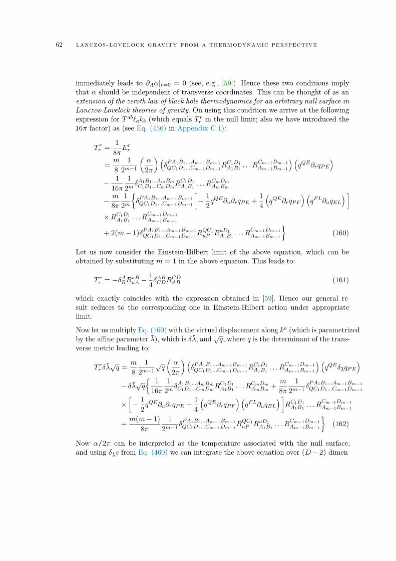
62 lanczos-lovelock gravity from a thermodynamic perspective

immediately leads to ∂Aα|r=0 = 0 (see, e.g., [59]). Hence these two conditions implythat α should be independent of transverse coordinates. This can be thought of as anextension of the zeroth law of black hole thermodynamics for an arbitrary null surface inLanczos-Lovelock theories of gravity. On using this condition we arrive at the followingexpression for T ab`akb (which equals T rr in the null limit; also we have introduced the16π factor) as (see Eq. (456) in Appendix C.1):

T rr =1

8πErr

=m

81

2m−1

(α

2π

)(δPA1B1...Am−1Bm−1QC1D1...Cm−1Dm−1

RC1D1A1B1

. . . RCm−1Dm−1Am−1Bm−1

) (qQE∂rqPE

)− 1

16π1

2m δA1B1...AmBmC1D1...CmDm

RC1D1A1B1

. . . RCmDmAmBm

− m

8π1

2mδPA1B1...Am−1Bm−1QC1D1...Cm−1Dm−1

[− 1

2qQE∂u∂rqPE +

14(qQE∂rqPF

) (qFL∂uqEL

) ]×RC1D1

A1B1. . . R

Cm−1Dm−1Am−1Bm−1

+ 2(m− 1)δPA1B1...Am−1Bm−1QC1D1...Cm−1Dm−1

RQC1uP RuD1

A1B1. . . R

Cm−1Dm−1Am−1Bm−1

(160)

Let us now consider the Einstein-Hilbert limit of the above equation, which can beobtained by substituting m = 1 in the above equation. This leads to:

T rr = −δABRuBuA −14δ

ABCDR

CDAB (161)

which exactly coincides with the expression obtained in [59]. Hence our general re-sult reduces to the corresponding one in Einstein-Hilbert action under appropriatelimit.

Now let us multiply Eq. (160) with the virtual displacement along ka (which is parametrizedby the affine parameter λ), which is δλ, and √q, where q is the determinant of the trans-verse metric leading to:

T rr δλ√q =

m

81

2m−1√q

(α

2π

)(δPA1B1...Am−1Bm−1QC1D1...Cm−1Dm−1

RC1D1A1B1

. . . RCm−1Dm−1Am−1Bm−1

) (qQEδλqPE

)− δλ√q

116π

12m δ

A1B1...AmBmC1D1...CmDm

RC1D1A1B1

. . . RCmDmAmBm+m

8π1

2m−1 δPA1B1...Am−1Bm−1QC1D1...Cm−1Dm−1

×[− 1

2qQE∂u∂rqPE +

14(qQE∂rqPF

) (qFL∂uqEL

) ]RC1D1A1B1

. . . RCm−1Dm−1Am−1Bm−1

+m(m− 1)

8π1

2m−1 δPA1B1...Am−1Bm−1QC1D1...Cm−1Dm−1

RQC1uP RuD1

A1B1. . . R

Cm−1Dm−1Am−1Bm−1

(162)

Now α/2π can be interpreted as the temperature associated with the null surface,and using δλs from Eq. (460) we can integrate the above equation over (D− 2) dimen-

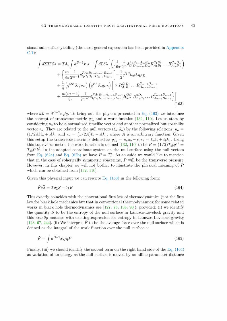
6.2 thermodynamic identity from gravitational field equations 63

sional null surface yielding (the most general expression has been provided in AppendixC.1): ∫

dΣT rr δλ = Tδλ

∫dD−2x s−

∫dΣδλ

[( 116π

12m δ

A1B1...AmBmC1D1...CmDm

RC1D1A1B1

. . . RCmDmAmBm

)+

m

8π1

2m−1 δPA1B1...Am−1Bm−1QC1D1...Cm−1Dm−1

[− 1

2qQE∂u∂rqPE

+14(qQE∂rqPF

) (qFL∂uqEL

) ]×RC1D1

A1B1. . . R

Cm−1Dm−1Am−1Bm−1

+m(m− 1)

8π1

2m−1 δPA1B1...Am−1Bm−1QC1D1...Cm−1Dm−1

RQC1uP RuD1

A1B1. . . R

Cm−1Dm−1Am−1Bm−1

](163)

where dΣ = dD−2x√q. To bring out the physics presented in Eq. (163) we introduce

the concept of transverse metric g⊥ab and a work function [132, 110]. Let us start byconsidering ua to be a normalized timelike vector and another normalized but spacelikevector ra. They are related to the null vectors (`a, ka) by the following relations: ua =(1/2A)`a + Aka and ra = (1/2A)`a −Aka, where A is an arbitrary function. Giventhis setup the transverse metric is defined as g⊥ab = uaub − rarb = `akb + `bka. Usingthis transverse metric the work function is defined [132, 110] to be P = (1/2)Tabgab⊥ =Tab`

akb. In the adapted coordinate system on the null surface using the null vectorsfrom Eq. (62a) and Eq. (62b) we have P = T rr . As an aside we would like to mentionthat in the case of spherically symmetric spacetime, P will be the transverse pressure.However, in this chapter we will not bother to illustrate the physical meaning of Pwhich can be obtained from [132, 110].

Given this physical input we can rewrite Eq. (163) in the following form:

F δλ = TδλS − δλE (164)

This exactly coincides with the conventional first law of thermodynamics (not the firstlaw for black hole mechanics but that in conventional thermodynamics; for some relatedworks in black hole thermodynamics see [127, 76, 138, 90]), provided: (i) we identifythe quantity S to be the entropy of the null surface in Lanczos-Lovelock gravity andthis exactly matches with existing expression for entropy in Lanczos-Lovelock gravity[123, 67, 244]. (ii) We interpret F to be the average force over the null surface which isdefined as the integral of the work function over the null surface as

F =∫dD−2x

√qP (165)

Finally, (iii) we should identify the second term on the right hand side of the Eq. (164)as variation of an energy as the null surface is moved by an affine parameter distance

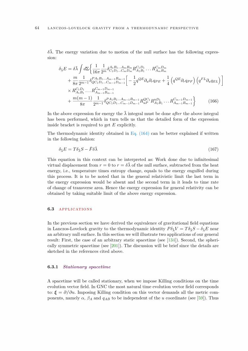
64 lanczos-lovelock gravity from a thermodynamic perspective

δλ. The energy variation due to motion of the null surface has the following expres-sion:

δλE = δλ

∫dΣ 1

16π1

2m δA1B1...AmBmC1D1...CmDm

RC1D1A1B1

. . . RCmDmAmBm

+m

8π1

2m−1 δPA1B1...Am−1Bm−1QC1D1...Cm−1Dm−1

[− 1

2qQE∂u∂rqPE +

14(qQE∂rqPF

) (qFL∂uqEL

) ]×RC1D1

A1B1. . . R

Cm−1Dm−1Am−1Bm−1

+m(m− 1)

8π1

2m−1 δPA1B1...Am−1Bm−1QC1D1...Cm−1Dm−1

RQC1uP RuD1

A1B1. . . R

Cm−1Dm−1Am−1Bm−1

(166)

In the above expression for energy the λ integral must be done after the above integralhas been performed, which in turn tells us that the detailed form of the expressioninside bracket is required to get E explicitly.

The thermodynamic identity obtained in Eq. (164) can be better explained if writtenin the following fashion:

δλE = TδλS − F δλ (167)

This equation in this context can be interpreted as: Work done due to infinitesimalvirtual displacement from r = 0 to r = δλ of the null surface, subtracted from the heatenergy, i.e., temperature times entropy change, equals to the energy engulfed duringthis process. It is to be noted that in the general relativistic limit the last term inthe energy expression would be absent and the second term in it leads to time rateof change of transverse area. Hence the energy expression for general relativity can beobtained by taking suitable limit of the above energy expression.

6.3 applications

In the previous section we have derived the equivalence of gravitational field equationsin Lanczos-Lovelock gravity to the thermodynamic identity PδλV = TδλS − δλE nearan arbitrary null surface. In this section we will illustrate two applications of our generalresult: First, the case of an arbitrary static spacetime (see [134]). Second, the spheri-cally symmetric spacetime (see [201]). The discussion will be brief since the details aresketched in the references cited above.

6.3.1 Stationary spacetime

A spacetime will be called stationary, when we impose Killing conditions on the timeevolution vector field. In GNC the most natural time evolution vector field correspondsto: ξ = ∂/∂u. Imposing Killing condition on this vector demands all the metric com-ponents, namely α, βA and qAB to be independent of the u coordinate (see [59]). Thus

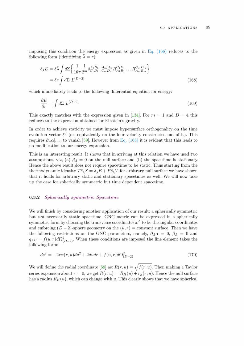
6.3 applications 65

imposing this condition the energy expression as given in Eq. (166) reduces to thefollowing form (identifying λ = r):

δλE = δλ

∫dΣ 1

16π1

2m δA1B1...AmBmC1D1...CmDm

RC1D1A1B1

. . . RCmDmAmBm

= δr

∫dΣ L(D−2) (168)

which immediately leads to the following differential equation for energy:

∂E

∂r=∫dΣ L(D−2) (169)

This exactly matches with the expression given in [134]. For m = 1 and D = 4 thisreduces to the expression obtained for Einstein’s gravity.

In order to achieve staticity we must impose hypersurface orthogonality on the timeevolution vector ξa (or, equivalently on the four velocity constructed out of it). Thisrequires ∂Aα|r=0 to vanish [59]. However from Eq. (168) it is evident that this leads tono modification to our energy expression.

This is an interesting result. It shows that in arriving at this relation we have used twoassumptions, viz, (a) βA = 0 on the null surface and (b) the spacetime is stationary.Hence the above result does not require spacetime to be static. Thus starting from thethermodynamic identity TδλS = δλE +PδλV for arbitrary null surface we have shownthat it holds for arbitrary static and stationary spacetimes as well. We will now takeup the case for spherically symmetric but time dependent spacetime.

6.3.2 Spherically symmetric Spacetime

We will finish by considering another application of our result: a spherically symmetricbut not necessarily static spacetime. GNC metric can be expressed in a sphericallysymmetric form by choosing the transverse coordinates xA to be the angular coordinatesand enforcing (D− 2)-sphere geometry on the (u, r) = constant surface. Then we havethe following restrictions on the GNC parameters, namely, ∂Aα = 0, βA = 0 andqAB = f(u, r)dΩ2

(D−2). When these conditions are imposed the line element takes thefollowing form:

ds2 = −2rα(r,u)du2 + 2dudr+ f(u, r)dΩ2(D−2) (170)

We will define the radial coordinate [59] as: R(r,u) =√f(r,u). Then making a Taylor

series expansion about r = 0, we get R(r,u) = RH(u)+ rg(r,u). Hence the null surfacehas a radius RH(u), which can change with u. This clearly shows that we have spherical

66 lanczos-lovelock gravity from a thermodynamic perspective

symmetry but have retained time dependence. Hence by imposing spherical symmetrythe energy satisfies a partial differential equation with the following form:

∂E

∂λ=∫dΣ 1

16π1

2m δA1B1...AmBmC1D1...CmDm

RC1D1A1B1

. . . RCmDmAmBm

+m

8π1

2m−1 δPA1B1...Am−1Bm−1QC1D1...Cm−1Dm−1

[− 1

2qQE∂u∂rqPE +

14(qQE∂rqPF

) (qFL∂uqEL

) ]×RC1D1

A1B1. . . R

Cm−1Dm−1Am−1Bm−1

+m(m− 1)

8π1

2m−1 δPA1B1...Am−1Bm−1QC1D1...Cm−1Dm−1

RQC1uP RuD1

A1B1. . . R

Cm−1Dm−1Am−1Bm−1

(171)

A much simpler form can be derived in which the 2-sphere line element is just (r +RH)2dΩ2

(D−2), where the radial coordinate at the null surface RH is a constant. Thentrading off r in favor of R the line element becomes

ds2 = −2 (R−RH)α(R,u)du2 + 2dudR+R2dΩ2(D−2) (172)

Then using the result that ∂uRH = 0, the differential equation for energy can beintegrated leading to,

E(R,u) =∫dλ

∫dΣ L(D−2) +X(u)

=1

16πAD−2RD−(2m+1)

2m∏j=2

(D− j) +X(u) (173)

where X(u) is an arbitrary function appearing as a “constant” of integration and AD−2originates from the differential volume element. Having introduced the radial coordinateR, we can replace λ by R, since R−RH = r, which coincides with the defining equationfor λ. As we move along ingoing radial lines, which are also ingoing radial null geodesic−∂/∂r, we will gradually hit the center of the (D− 2)-spheres (assuming that it exists).The affine parameter at the center would be R = 0. Then Eq. (173) at the center turnsout to be:

E(R = 0,u) = X(u) (174)

Since the center is a single point it is natural to associate zero energy with it, whichdetermines the arbitrary function to be X(u) = 0. Thus substituting this result inEq. (173) and evaluating on the null surface, we obtain the energy associated with thenull surface in a spherically symmetric spacetime to be given by

E =1

16πAD−2RD−(2m+1)H

2m∏j=2

(D− j) (175)

This again matches exactly with the result obtained in [201]. Another important thingto note is the following: the expression for energy, first obtained for static sphericallysymmetric configuration also holds for time dependent situation with only sphericalsymmetry assumed.

6.4 thermodynamic interpretations in lanczos-lovelock gravity 67

6.4 thermodynamic interpretations in lanczos-lovelock grav-ity

As we have mentioned earlier, in this chapter we will be dealing exclusively withLanczos-Lovelock gravity. We will provide a generalization of a four vector from Ein-stein gravity to Lanczos-Lovelock gravity, which will carry the notion of gravitationalmomentum. Then we will concentrate on variation of this momentum and its mean-ing in thermodynamic language. Finally we discuss the null surfaces in the context ofLanczos-Lovelock gravity.

6.4.1 Bulk Gravitational Dynamics And Its Relation to Surface Thermo-dynamics in Lanczos-Lovelock Gravity

In [190] it has been illustrated that, total energy of matter and gravity equals thesurface heat content in the context of general relativity. To prove this a suitably definedgravitational four-momentum P a has been used such that when integrated over a t =constant surface with proper integration measure it leads to a notion of gravitationalenergy. The notion of energy is quiet ambiguous in the sense of observer dependence.For example, even in special relativity the energy of a particle with four momentump as measured by an observer with four velocity u is: E = −u.p. This immediatelysuggests that we should use identical trick to identify the energy by contracting asuitably defined four momentum P a with the four velocity ua = −N∇at, normal tot = constant surface. We will first briefly describe the situation for general relativityand shall generalize subsequently to Lanczos-Lovelock gravity.

Bulk Energy Versus Surface Heat Energy The Einstein-Hilbert action canbe written explicitly in terms of two canonically conjugate variables, namely, fab =√−ggab and N c

ab = QcpaqΓqbp +QcpbqΓqap [203]. It turns out that the Einstein-Hilbert ac-

tion can be interpreted as a momentum space action with fab as the coordinate andN cab as its conjugate momentum [203]. Using these two variables a natural definition

of gravitational momentum can be provided as (Note that the negative sign in front ofP a is just a convention, such that −uaP a relates to the energy.):

−P a(q) = gij£qNaij + qaL (176)

where qa is an arbitrary vector field. This follows from the result that Hamiltoniancan be written as H = qp+ L with the identification of p as N c

ab and q as gab (or fabif we consider −√−gP a). However in order to generalize the above result to Lanczos-Lovelock gravity, we should rewrite the above expression in a slightly modified form,such that: gij£qN

aij = 2gij£q(Q

apimΓmjp) = 2Q jpa

m £qΓmjp. Thus the above action can alsobe interpreted with Γmjp and Q jpa

m as conjugate variables. Surprisingly, this is also avalid pair of conjugate variables as illustrated in [56] and can be generalized readily toLanczos-Lovelock gravity. However in this case we need to interpret Γmjp as the momentaand Q jpa

m as the coordinate, which is true since Γmjp has 40 independent degrees offreedom while Q jpa

m as constructed out of the metric only has 10 independent degreesof freedom (a detailed discussion has been presented in [56]). The above setup can be

68 lanczos-lovelock gravity from a thermodynamic perspective

generalized in a natural fashion to Lanczos-Lovelock gravity following [56] and leadsto:

−√−gP a(q) = 2

√−gP qra

p £qΓpqr +√−gLqa (177)

The physical structure of this momentum can be understood in greater detail by us-ing the Noether current. Writing the corresponding expression for Noether currentexplicitly in the case of Lanczos-Lovelock gravity and then simplifying we obtain (seeAppendix C.2.1):

Ja(q) = ∇bJab(q) = 2Eab qb − P a(q) (178)

This leads to another definition for the momentum which will turn out to be quietuseful and can be given as,

−P a(q) = ∇bJab(q)− 2Eab qb (179)

Then divergence of the momentum has the following expression:

∇aP a(q) = 2Eab∇aqb (180)

in arriving at the above expression we have used two results, Noether potential Jabbeing antisymmetric and Eab satisfying Bianchi identity. From the expression it isevident that if we enforce field equations for pure gravity, which amounts to: Eab = 0,the momentum becomes divergence free. Also appearance of Noether current explicitlyin this expression shows intimate connection of Noether current with energy in allLanczos-Lovelock models of gravity.

So far the results are completely general, holding for any vector field qa. Now wewill specialize to the vector field ξa and will show that it leads to several remarkableresults. First we start with momentum for ξa and its contraction with ua leading to(see Appendix C.2.1):

−uaP a(ξ) = Dα (2Nχα)− 2NEabuaub (181)

where the vector χa is defined in Eq. (141). Now using the equation of motion i.e. 2Eab =Tab and integrating the above expression on a t = constant surface bounded by N =constant surface we get the following expression (16π factor has been introduced):∫

RdD−1x

√hua

−P a(ξ) +NT ab u

b=∫∂R

dD−2x Tlocs (182)

The expression on the left hand side represents total, i.e., matter energy plus gravi-tational energy in a bulk region and the right hand side represents the heat contentof the boundary surface. The temperature as usual is given by: Na/2π, i.e., the red-shifted Unruh-Davies temperature and s is the Wald entropy density associated withthe boundary surface. The right hand side of the above expression can also be identi-fied as half of the equipartition energy of the boundary surface. Hence the bulk energyoriginating from both gravity and matter is equal to the surface heat content.

6.4 thermodynamic interpretations in lanczos-lovelock gravity 69

Variation of Gravitational Energy From the above paragraph it is clear that themomentum P a and the corresponding gravitational energy −uaP a(ξ) have very inter-esting thermodynamic properties. In this light, it seems natural to consider variationof the above momentum under various physical processes, e.g., how it changes due toprocesses acting on the boundary. We will first work with the arbitrary vector field qaand then we will specialize to the choice: qa = ξa. To our surprise just as in generalrelativity even in Lanczos-Lovelock gravity variation of the gravitational momentum isconnected to symplectic structures [125, 208].

Thus by variation of −√−gP a(q) and manipulating the terms carefully we obtain thesymplectic structure as (see Appendix C.2.1)

−δ (√−gP a) =

√−gEpqδgpqqa +

√−gωa + ∂c

(2√−gP qr[a

p qc]δΓpqr)

(183)

where the symplectic form ωa has the following expression:√−gωa (δ, £q) = δ

(2√−gP qra

p

)£qΓpqr −£q

(2√−gP qra

p

)δΓpqr (184)

This expression is true for any arbitrary vector field qa and involves one arbitraryvariation and another Lie variation along qa.

Having obtained the general result we will now specialize to the vector field ξa. Thenwe can use the above formalism in order to obtain the change in gravitational energyof the system due to its evolution, which is related to Lie derivative along ξa. Thiscan be achieved using a simple trick. First with the help of Eq. (184) we can computethe object δ[−

√huaP

a(ξ)]. The variation has the following expression (see AppendixC.2.1):

−δ[√huaP

a(ξ)]+√−gEpqδgpq =

√huaω

a + ∂c[2√−ghcaP qra

p δΓpqr]

(185)

This holds for an arbitrary variation, however what we are interested in is when theabove variation is due to a diffeomorphism along ξa. Again from Appendix C.2.1 usingthe field equation 2Eab = Tab we arrive at:

£ξHgrav = £ξ

(−∫RdD−1x

√huaP

a(ξ)

)=∫∂R

dD−2x√qNra

(T cdξd + 2P qra

p £ξΓpqr)

(186)

where ra is the unit normal to N = constant surface within the t = constant surfaceand Hgrav stands for integral of −

√huaP

a(ξ) over the (D − 1)-dimensional volume.Hence change of energy in the bulk is directly related to boundary effects (with theassumption that T tcξc = 0). Among the two terms present on the right hand side, thefirst term is due to flow of matter energy across the boundary and the second term isrelated to our old friend P qra

p £ξΓpqr. For pure gravity, i.e., Tab = 0, the above resulttakes a much simpler form as:

£ξHgrav =∫∂R

dD−2x√qNra2P qra

p £ξΓpqr (187)

70 lanczos-lovelock gravity from a thermodynamic perspective

This can have direct influence on gravity wave propagation, i.e., the energy changein a bulk region due to gravity waves is related to surface processes and hence toP qrap £ξΓpqr.

Since the gravitational momentum is intimately connected to Noether current, we canuse the above results for variation of gravitational momentum in order to obtain a vari-ation of Noether current as well. From Appendix C.2.1 on imposing on-shell condition,i.e., Eab = 0, we get:

√huaω

a (δ, £q) + 2δ(√

huaEabqb

)= ∂b

δ[√huaJ

ab(q)]− 2√huaP

qr[ap qb]δΓpqr

(188)

This expression can be related to the usual Hamiltonian formulation where one relatesbulk integral of δ(HN +HαN

α) (with H and Hα correspond to constraints in thegravity theory; N and Nα are the standard ADM variables) to a bulk and a surfacecontribution as:

δ

∫RdD−1x

√h(HN +HαN

α) =∫RdD−1xδB +

∫∂R

dD−2xδS (189)

The variation present on the left hand side is equivalent to δ(2√huaE

abζb), whereζa = Nua + Na, with Na = (0,Nα). Then we can identify the bulk term on theright hand side with the symplectic current ωa. Thus finally the remaining surfacecontribution turns out to be:∫

∂RdD−2xδS =

∫∂R

dD−2xrbδ[√huaJ

ab(ζ)]− 2√h(NP qra

p + P qr[ap N b]

)δΓpqr

(190)

This provides an elegant and simple interpretation of the surface term appearing in thevariation of the gravitational action. Thus for Lanczos-Lovelock gravity the Hamiltonianformulation as well can have thermodynamic counterpart.

The above approach of relating surface quantities with bulk energy has also been studiedearlier, notably in the context of Virasoro algebra and its associated central charge [46].In [155] the above approach has been used to derive Wald entropy in Lanczos-Lovelocktheories of gravity, which subsequently has been generalized in [153] in order to calculatecorrection to horizon entropy in higher derivative gravity theories. It has been shownin this context that surface contribution alone is what will lead to the central chargeand hence to horizon entropy. Our result strengthens the above feature by showinga connection between total energy and boundary heat energy in all Lanczos-Lovelocktheories of gravity.

6.4.2 Heat Density of the Null Surfaces

In this final section we will discuss heat density associated with a null surface in Lanczos-Lovelock gravity. Any null surface will be defined using a congruence of null vector `a,which are tangent as well as normal to the null surface. We will also assume that the nullvector `a satisfies the relation `2 = 0, everywhere. The null congruence will be taken

6.4 thermodynamic interpretations in lanczos-lovelock gravity 71

to be non-affinely parametrized, such that, `a = A(x)∇aB(x). Then the non-affinityparameter κ can be obtained from the relation:

`j∇j`i = κ`i; κ = `i∂i lnA (191)

Since the null vector is both tangent and orthogonal, in order to define a projectionwe need an auxiliary null vector ka [202] with the following properties k2 = 0 andka`

a = −1. Then we can introduce a projection tensor qab = δab + `akb+ `bka and define

an associated covariant derivative Da.

In the previous sections we have calculated Noether current for ξa and its contractionwith ua yielding Noether charge. In the context of null surfaces we will discuss Noethercurrent for `a and its contraction with `a itself. This leads to (see Appendix C.2.2)

`aJa(`) = ∇a (K`a)− κK (192)

where we have introduced the object K = −2P abcd`akb`d∇c lnA. This in the generalrelativity limit coincides with κ. Note the formal similarity of the expression on theright hand side, i.e., ∇a (K`a)− κK for null surface to the expression Dαχ

α = ∇iχi −ajχ

j obtained for spacelike surface. Also the expression for χa is quiet similar to theexpression for K with `a and ka identified with ua and ra respectively. Then introducingthe covariant derivative Da on the surface the above expression can be written as (seeAppendix C.2.2)

`aJa(`) = 2Rab`a`b + 2`aP qra

p £`Γpqr = Da (K`a) +dKdλ

(193)

Integrating the above expression over the null surface with integration measure dλdD−2x√q

and ignoring the boundary contribution we arrive at:∫dλdD−2x

√q`aJ

a(`) =∫dλdD−2x

√qdKdλ

(194)

This result at the face value shows that for the null surface contraction of the Noethercurrent along `a is related to heating of the boundary surface, with K being taken astemperature in the Lanczos-Lovelock gravity.

This result is also important from the point of view of variational principle for null sur-faces. Such a variational principle based on null surfaces has been carefully investigatedin [195]. Following that, given a null surface with null congruence `a we can constructthe functional

Q =∫ λ2

λ1dλdD−2x

√q (−2Rab + Tab) `

a`b (195)

Then varying the above action functional with respect to all `a with the constraint`2 = 0, we will arrive at: Rab − (1/2)T ab = f(x)δab . This on using Bianchi identity,∇aEab = 0 = ∇aT ab leads to gravitational field equations with an undeterminedcosmological constant originating from integration constant.

72 lanczos-lovelock gravity from a thermodynamic perspective

Then from Eq. (193) we can write Rab`a`b in terms of Lie derivative of the connectionand change of K along the null geodesics such that

−2Rab`a`b = 2`aP qrap £`Γpqr −

[Da (K`a) +

dKdλ

](196)

Then substitution of−2Rab`a`b on the right hand side of Eq. (195) leads to the followingmodified variational principle for Lanczos-Lovelock gravity when boundary terms areneglected as

Q =∫ λ2

λ1dλdD−2x

√q

[(2`aP qra

p £`Γpqr −dKdλ

)+ Tab`

a`b]

(197)

Hence varying this Lagrangian with respect to `a with `2 = 0, we can obtain the fieldequation for gravity with an arbitrary cosmological constant. In the above expressionTab`

a`b can be taken as matter heat density Ts, while the rest of the terms representheat density of the null surface itself.

We can always choose the parameter λ such that the null vector `a is affinely parametrized.In which case K = 0 and the variational principle can be based on the following inte-gral:

Q =∫ λ2

λ1dλdD−2x

√q[2`aP qra

p £`Γpqr + Tab`a`b]

(198)

Again showing explicitly the importance of the Lie derivative term in the derivationof the field equations from an alternative action principle. When there is no matterpresent the variational principle simplifies considerably leading to

Q =∫ λ2

λ1dλdD−2x

√q[2`aP qra

p £`Γpqr]

(199)

This leads to vacuum field equations when varied over all null surfaces simultaneously.Also integral of this object has an interpretation of heat content over the boundary sur-face. Thus we observe that at least for affinely parametrized null congruences the vari-ational principle over the null surface acquires a thermodynamic interpretation.

6.5 discussion

In this chapter our aim was to generalize various results derived in the context of generalrelativity to all Lanczos-Lovelock theories of gravity. This is a non-trivial task sincethe Lanczos-Lovelock Lagrangian contains higher order terms constructed out of thecurvature tensor. Also validity of some result in general relativity does not guarantee itsvalidity in these higher curvature theories, e.g., the expression for entropy in generalrelativity does not hold in Lanczos-Lovelock gravity. Let us now summarize the keyresults obtained through this exercise:

• In Section 6.2 we have shown that the field equations for Lanczos-Lovelock gravitynear an arbitrary null surface is equivalent to a thermodynamic identity. Usinga parametrization (known as GNC) for the arbitrary null surface we have shownthat the field equations for Lanczos-Lovelock gravity can be used to relate energy

6.5 discussion 73

momentum tensor with thermodynamic features. This exercise also provides us adefinition of energy in an arbitrary spacetime in Lanczos-Lovelock gravity, whichin the static case and spherically symmetric case reduces to standard energydefinitions.

• Next, in Section 6.4.1 we have introduced a gravitational momentum starting fromits expression in general relativity. Using this gravitational momentum we haveshown that total gravitational plus matter energy in a bulk volume equals the heatdensity associated with the boundary surface. Also variation of the gravitationalHamiltonian is directly related to a symplectic structure such that time evolutionof this gravitational Hamiltonian in a bulk region can be related to surface effectsespecially with P qra

p £ξΓpqr. Using this formalism it is also possible to connectstandard Hamiltonian formalism with the thermodynamic features discussed here.

• Finally, in Section 6.4.2 we have discussed an alternative variational principle forthe null surfaces in Lanczos-Lovelock gravity. It turns out that the variationalprinciple has a nice separation into matter heat density and gravitational heatdensity associated with the null surface. In this case as well for affine parametriza-tion of null vectors and in vacuum spacetime, i.e., with no matter, the actionfunctional is simply 2√−gP qra

p £ξΓpqr. This provides yet another thermodynamicinterpretation for this Lie variation term.

All these results suggest the importance of Noether current in any Lanczos-Lovelocktheories of gravity and its relation to the thermodynamic features.

7NULL SURFACE GEOMETRY AND ASSOCIATEDTHERMODYNAMICS

7.1 introduction

The development of emergent gravity paradigm has helped us to understand severalinteresting features of classical gravity itself [183], further bolstering our confidence inthe veracity of this approach. In particular, the curious relationship between Einstein’sfield equations and the structure of null surfaces in the spacetime. Previous works haveshown that they manifest in three different ways:

• In the most general situation, there arises an identification between Navier-Stokesequation and Einstein’s equations. Einstein’s equations, when projected on anarbitrary null surface, in any spacetime, leads to Navier-Stokes equation of fluiddynamics [186, 131].

• From the Einstein’s equations applied to a null surface, one can get [176, 40, 4,137, 201] a thermodynamic identity of the form TδλS = δλE+PδλV in which thesymbols have their usual meanings and the variation can be interpreted as changesdue to virtual displacement of the null surface along null geodesics parametrizedby the affine parameter λ off the surface. Initially proved for a few configurationswith a high level of symmetry [201, 134] this result has now been generalized forarbitrary null surfaces in both general relativity and Lanczos-Lovelock theoriesof gravity [59, 54].

• A comparatively more approximate relationship between the null surfaces andEinstein’s equations emerged from the early work [122], which ‘derived’ Einstein’sfield equations using the local Rindler horizon as a null surface and the Clausiusrelation. This relies heavily on the structure of Raychaudhuri equation as wellas the assumptions: (a) the entropy density is one quarter of the transverse areaand, more importantly, (b) the quadratic terms in the Raychaudhuri equation(involving the squares of shear and expansion) can be set to zero. Since neitherthe Raychaudhuri equation nor the assumption that entropy is proportional to thehorizon area hold for theories more general than Einstein’s gravity, this approachcould not be generalized in a simple manner to more general class of theories.

In this chapter, we shall revisit these issues and elaborate further on them using an-other recent development, which was also motivated by the emergent gravity paradigm.The chapter is organized as follows: In Section 7.2 we discuss the Noether current andthe associated thermodynamic results for both the (1+3) foliation and the Gaussiannull coordinates. The thermodynamic interpretation of the reduced gravitational mo-mentum is given in Section 7.3. The final section, i.e., Section 7.4 discusses the threedifferent projections of the gravitational momentum vis-á-vis a null surface and their

75

76 null surface geometry and associated thermodynamics

thermodynamic interpretation. We end the chapter with a short discussion on our re-sults.

7.2 noether current and spacetime thermodynamics: null sur-faces

There exists two natural foliations of the spacetime, one based on the (1+3) split andthe other adapted to a fiducial null surface. These coordinate charts also come withcertain natural vector fields. In the case of the (1+3) split, the time evolution is relatedto the vector field ξa introduced in [190]. In the case of the foliation based on a nullsurface, we again have a natural time evolution field ξa given by Eq. (55) as well asthe null vector `a which is tangent to the null congruence defining the null surface.It would be interesting to study the Noether current and the gravitational momentacorresponding to the vector fields associated with null surfaces, which turn out tohave direct thermodynamic significance. In this section we shall consider the Noethercurrents; we will take up the properties of gravitational momenta in Section 7.4.

Let us consider the corresponding thermodynamic interpretation of the Noether currentwhen we use the time development vector field adapted to the null surface in the GNC.To begin with one can consider the result — Noether charge contained in a bulk regionequals the heat content of the boundary, however derived for a subregion of a spacelikesurface. It turns out that a similar result holds for a null surface as well. Given the factthat the Noether current corresponding to the time development vector led to a nicethermodynamic interpretation, we will consider the object `aJa(ξ). (In GNC ξa hasthe components as in Eq. (55) and `a is given by Eq. (62a), but of course our resultsare covariant.). It then turns out that (see Eq. (566) of Appendix D.3),

16π`aJa(ξ) = Jr(ξ) =1√q

d

dλ(2α√q) (200)

where λ is the parameter along the null generator `a, which in GNC is simply u and wehave reintroduced the 16π factor. This equation can be integrated over the null surfacewith integration measure √qd2xdλ and leads to,

∫d2xdλ

√q`aJ

a(ξ) =∫d2x

(α

2π

)(√q

4

) ∣∣∣∣λ=λ2

λ=λ1

= Q(λ2)−Q(λ1) (201)

where

Q(λ) =∫d2x

(α

2π

)(√q

4

)=∫d2xTs (202)

is the heat content of the null surface at a given λ.

This again shows that total Noether charge density for the vector field ξa integratedover the null surface equals the difference of the heat content Q of the two dimensionalboundaries located at λ = λ2 and λ = λ1. Previously the connection between bulkNoether charge to surface heat density was derived in the context of spacelike surfaces.The result in Eq. (201) generalizes the previous connection — between bulk Noethercharge and surface heat density in the context of spacelike surfaces — by showing that

7.2 noether current and spacetime thermodynamics: null surfaces 77

the total Noether charge on a null surface is also expressible as the heat content of theboundary.

The following aspect of this result is worth highlighting. We have mentioned earlier tworesults (see Eq. (117) and Eq. (432)) of similar nature. The first one (see Eq. (117)) wasfor a spatial region V contained in a space-like hypersurface. In that case, the normalto the surface was ua and the natural integration measure, for integrating the normalcomponent of a vector field is ua

√h d3x. We computed the integral Jaua

√h d3x and

found that it is given by a boundary term; we could have also computed the integralin a region contained within two boundary surfaces like, for example, in the shell-likeregion between two spherical surfaces of radii R1 and R2. We would have then foundthat the Noether charge in the bulk region is the difference between the heat contentsof the two surfaces.

In the second case, (see Eq. (432) in Appendix B) we considered the flux of Noethercurrent through a timelike surface with normal ai. In this case we calculated the integralof apJp(ξ) with the measure d2xdt

√−g⊥ on a timelike surface and got a similar result.

We also mentioned that in this case, the integrand apJp(ξ) is to be thought of as heatflux per unit time.

In the case of a null surface, our result is similar to the second one, given by Eq. (432).Now the corresponding integration measure for integrating a vector field over a nullsurface is given by `a

√q d2x dλ where `a = dxa/dλ is the tangent vector to the null con-

gruence defining the null surface. Therefore, in this case, we calculate the integral overJa`a√q d2x dλ. This leads to the difference ∆Q of the heat content at the two bound-

aries corresponding to λ = λ1 and λ = λ2. In the integrand in this case, Ja`a√q d2x dλ

one of the coordinates λ is similar to a time coordinate rather than a spatial coordinate.So we cannot think of Ja`a as charge per unit volume; instead it represents charge perunit area (flux) per unit time and more appropriately, it is the rate of production ofheat per unit area of the null surface.

It is possible to proceed further and relate the change in the heat content with thematter energy flux through the null surface. To do this, we use Eq. (34) and fieldequation Gab = 8πTab to obtain (on the null surface):

16πTab`a`b = 16π`aJa(ξ)− `agbc£ξNabc (203)

The Lie derivative term can be computed directly to give (see Eq. (604) of AppendixD.3):

√q`ag

ij£ξNaij = −qab£ξΠab +

d2√qdλ2 (204)

where Πab =√q[Θab − qab(Θ + κ)] is the momentum conjugate to qab and Θab =

qamqbn∇m`n where Θ is the trace of Θab. Integrating this result over the null surface

between λ = λ1 and λ = λ2, and assuming for simplicity that the boundary terms atλ = λ1,λ2 do not contribute (which assumes dA/dλ = 0 at the end points where A isthe area of the null surface), we get:

− 116π

∫d2xdλ qab£ξΠab = [Q(λ2)−Q(λ1)]−

∫dλd2x

√qTab`

a`b (205)

78 null surface geometry and associated thermodynamics

This expression shows that the evolution of the spacetime, which is encoded by theevolution of the momentum Πab is driven by the difference between (i) heat contentQ at the boundary and (ii) the matter heat flux flowing into the null surface. We canrewrite this in a nicer manner as follows. We define the surface degrees of freedomas:

Nsur = A =∫d2x√q (206)

and the average temperature as:

Tavg =1A

∫d2x√q

(α

2π

)(207)

We also introduce the effective bulk degrees of freedom by:

Nbulk =1

(1/2)Tavg

∫dλd2x

√q2Tab`a`b (208)

If the matter heat flux, given by the integral in the right hand side, thermalizes atthe average temperature of the null surface then, Nbulk will represent the effectiveequipartition degrees of freedom. We now rewrite Eq. (205) as,

− 18π

∫d2xdλ qab£ξΠab =

12

∫λ2d2x

(α

2π

)√q− 1

2

∫λ1d2x

(α

2π

)√q

− 2∫dλd2x

√qTab`

a`b (209)

which, on using our definitions, becomes:

− 18π

∫d2xdλ (qab£ξΠab) =

12Tavg

[(Nsur)

λ2λ1−Nbulk

](210)

This has the interpretation that the evolution of spacetime on a null surface, encodedin the Lie variation of the momentum Πab along the time development vector, canbe thought of as due to the difference between surface degrees of freedom and thebulk degrees of freedom. This an exact analogy to the corresponding result in (1 + 3)foliation presented in Eq. (118), which was originally obtained in [190].

For the sake of completeness, we clarify the notion of Tab`a`b being the heat flux throughthe null surface. This concept has been introduced in [122] and arises as follows: Letthere be a matter field, in the spacetime, with energy momentum tensor Tab. Aroundany given spacetime event P, we can construct local inertial and hence local Rindlerframes. We then have an approximate Killing vector field ξa, generating boosts, whichcoincides with the null normal `a at the null surface. The heat flow vector is defined asthe boost energy current obtained by projecting Tab along ξb yielding Tabξb. Thus theenergy (heat) flux through the null surface will be:

Q =∫ (

Tabξb)dΣa =

∫Tabξ

b`a√qd2xdλ (211)

where √qd2xdλ is the integration measure on a null surface generated by null vectors`a, parametrized by λ. Hence, in the null limit, Tab`a`b (when ξa → `a on the nullsurface) represents the heat flux through the null surface.

7.3 reduced gravitational momentum and time development vector 79

The same argument can also be presented along the following lines. On a null surfacewe can decompose Tabξb in canonical null basis as, Tabξb = A`a +Bka + CAe

Aa . Then

the heat flux through the surface is given by the component B along ka, which is off thenull surface. This component B is obtained by contracting with `a (since `2 = 0 and`ak

a = −1). This leads to the heat flux through the null surface to be Tab`a`b.

7.3 reduced gravitational momentum and time development vec-tor

In Chapter 2 we have introduced both the Noether current and the gravitational mo-mentum for general relativity, while the same for Lanczos-Lovelock gravity has beenintroduced in Chapter 2 and Chapter 6 respectively. In all these cases we notice thatthe combinations

Pa = −gij£vNaij ; Pa = −2P qra

p £vΓpqr (212)

appear quite naturally in them. We shall call this combination reduced gravitationalmomentum Pa. (We will see later that Pa is closely related to the rate of productionof heat per unit area on null surfaces.)

The algebraic reason for the occurrence of this combination is as follows. It turns outthat, in the thermodynamic interpretation of gravity, the combination Tab = Tab −(1/2)Tgab occurs more naturally than the energy momentum tensor Tab, with the fieldequations often arising [190, 55] in the form 2Rab = Tab rather than as 2Gab = Tabin Einstein’s gravity. The total momentum of gravity plus matter can be expressed,on-shell, in the form:

(P a +Ma) = −gij£vNaij −Rva − T ab vb

= −gij£vNaij +

12Tδ

ab v

b − T ab vb

= −gij£vNaij − T ab vb ≡ (Pa + Ma) (213)

where Ma = −T ab vb is the matter momentum associated with T ab . This shows that thevector Pa = −gij£vN

aij bears the same relation to T ab as P a does with T ab . Just as

T ab appears more naturally in the emergent gravity paradigm, the Pa will also appearrepeatedly in our discussions.

The notion of reduced gravitational momentum can also be generalized to the Lanczos-Lovelock models as well. For pure m-th order Lanczos-Lovelock gravity we have therelation 2[m− (D/2)]L = T . So we can write,

(P a +Ma) = −2P qrap £vΓpqr −Lva − T ab vb

= −2P qrap £vΓpqr −

12[m− (D/2)]Tδ

ab v

b − T ab vb

= −2P qrap £vΓpqr − T ab vb ≡ Pa + Ma (214)

where the reduced gravitational momentum is naturally defined as

Pa = −2P qrap £vΓpqr (215)

80 null surface geometry and associated thermodynamics

In the case of general relativity, the gravitational momentum Pa defined in Eq. (215)goes over to the −gij£vN

aij term, as it should.

The expression for the Noether current contains a Lie derivative term which was definedearlier as the reduced gravitational momentum. In this section, we shall describe somekey properties of this reduced gravitational momentum vector in different contexts,emphasising the results in GNC.

In the case of (1+3) foliation using spacelike surfaces with normal ua = −N∇at (Nis the lapse function) and induced metric hab = gab + uaub the reduced gravitationalmomentum can be related [190] to the Lie variation of pab =

√h(Khab−Kab) by:

−√huaPa(ξ) =

√huag

ij£ξNaij = −hab£ξp

ab (216)

where, ξa = Nua, is associated with the (1 + 3) foliation of the spacetime (see e.g.,[190]).

In the case of null surfaces, one can obtain a similar relation. For a general, non-affineparametrization, i.e., when the null generator `a satisfy the relation `b∇b`a = κ`a, wefind that the Lie variation term is given by (see Eq. (604) of Appendix D.3):

−√q`aPa(ξ) =√q`ag

ij£ξNaij = −qab£ξΠab +

d2√qdλ2 (217)

where Πab =√q[Θab − qab(Θ + κ)] is the momentum conjugate to qab. Here, ξa is the

time evolution vector associated with null foliations, such that ξa → `a as the nullsurface is approached (in particular, see also Eq. (55)). Thus as in the case of thespacelike surface, for null surfaces as well, the Lie variation of N c

ab is directly related tothe Lie variation of the momentum conjugate to the induced metric on the null surface.But in the case of null surfaces there is an extra term which contributes only at theboundaries λ = λ1,λ2.

It can be seen from straightforward algebra (see Eq. (536) of Appendix D.1) thatqab£ξΠab is directly related to the object D = ΘabΘab−Θ2 defined in Eq. (543), whichcan be interpreted as dissipation [131]. This leads to an alternative expression on thenull surface for the Lie variation term in the adapted coordinate system as (see Eq. (589)and Eq. (603) in Appendix D.3),

`agij£ξN

aij = 2D+

2√q∂2λ (√q) + 2∂λα (218)

Integrating this expression over the r = 0 null surface with integration measure d2xdu√q,

neglecting total divergence and dividing by 16π leads to,

116π

∫d2xdλ

√q`ag

ij£ξNaij =

18π

∫d2xdλ

√qD+

∫d2x

(√q

4

)d

(α

2π

)(219)

which explicitly shows that the Lie variation term integrated over the null surface,leads to the dissipation and the sdT term (interpreted as dT = (dT/dλ)dλ). Hencethe reduced gravitational momentum on the null surface, can be given a natural ther-modynamic interpretation.

7.4 projections of gravitational momentum on the null surface 81

What is important regarding the above result is that for ∂λqab = 0 (i.e., the inducedmetric on the null surface is independent of the parameter along the null generator)the dissipation term vanishes and thus Eq. (219) can be written as:

116π

∫d2xdλ

√q`ag

ij£ξNaij = Q(λ2)−Q(λ1) (220)

Hence the Lie variation term in this particular situation is equal to difference in theheat content allowing us to relate Pa to the rate of heating of the null surface.

7.4 projections of gravitational momentum on the null surface

We shall now take up a further application of the concept of gravitational momentum.Given the thermodynamic significance of the null surfaces, we would expect the flowof gravitational momentum vis-á-vis a given null surface to be of some importance. Toexplore this, we have to first choose a suitable vector field using which the gravitationalmomentum can be defined. The most natural choice — as before — is the time evolutionfield ξa. Further, in the canonical null basis (`a, ka, eaA) the gravitational momentumcan be decomposed as: P a = A`a +Bka +CAeaA. These components A,B and CA arerelated to the three projections of P a by A = −P a(ξ)ka, B = −P a(ξ)`a and CA =P a(ξ)eAa . So we need to consider the following three components qabP b(ξ), kaP a(ξ) and`aP

a(ξ) to get the complete picture. We will see that each of them lead to interestingthermodynamic interpretation. In view of the rather involved calculations, we will firstprovide a summary of the thermodynamic interpretations of these projections:

• The component qbaP a(ξ) leads to the Navier-Stokes equation for fluid dynam-ics, using which we can obtain yet another justification for the dissipation termintroduced in Eq. (543). This is described in Section 7.4.1

• The component kaP a(ξ), when evaluated on an arbitrary null surface leads to aresult which can be stated in the form: TdS = dE + PdV , i.e., as a thermody-namic identity. This helps us to identify a notion of energy associated with anarbitrary null surface. We obtain this result in Section 7.4.2.

• Finally, the component `aP a(ξ) yields the evolution of null surface, which involvesboth ds/dλ and dT/dλ, where s is the entropy density and T is the temperatureassociated with an arbitrary null surface and λ is the parameter along the nullgenerator `a. This is studied in Section 7.4.3.

We shall now show how all these three results tie up with the notion of gravitationalmomentum and arise naturally from the three different projections of the gravitationalmomentum.

7.4.1 Navier-Stokes Equation

The equivalence of field equations for gravity, when projected on a null surface, andthe Navier-Stokes equation is an important result in the emergent paradigm of gravity.This result, which generalizes the previous one [69] in the context of black holes, showsthat when Einstein’s equations are projected on any null surface and viewed in local

82 null surface geometry and associated thermodynamics

inertial frame, they become identical to the Navier-Stokes equation of fluid dynamics[186]. Here we will project the gravitational momentum P a on an arbitrary null surfaceparametrized by GNC and show that the Navier-Stokes equation is obtained. For thispurpose we will consistently use the vector field ξa. Even though we will present theresults for the adapted coordinates to a null surface (i.e., in GNC), the same resultcontinues to hold in any other parametrization as well.

In order to project the gravitational momenta −16πP c(ξ) = gab£ξNcab + Rξc on the

null surface we need to determine the induced metric qab , which [202] turns out to bediag(0, 0, 1, 1). Hence it is the angular part which is going to contribute. The vectors `aand ka are already given in Eq. (62a) and Eq. (62b) respectively. In the Navier-Stokesequation two other vectors play a crucial role. These vectors and their components inthe adapted GNC system has the following expressions:

ωb = `m∇mkb =(α, 0, 1

2βA)

; ωa =

(0,α, 1

2βA)

(221)

and

Ωa = ωa + αka =

(0, 0, 1

2βA)

; Ωa =

(0, 0, 1

2βA)

(222)

From [186] we know that βA can be interpreted as the transverse velocity of observerson the null surface. (In particular it can be interpreted as velocity drift of local Rindlerobservers parallel to the Rindler horizon.) With this physical motivation, let us nowstart calculating the projection of P a on the null surface. Using the coordinates adaptedto a given null surface, we arrive at:

−16πqabP b(ξ) = qab gpq£ξN

bpq = 2£ξN

Aur + qBC£ξN

ABC (223)

where we have used the identity `aqab = 0. We next need to find the Lie variation ofN cab. For that we use the expression £vΓabc = ∇b∇cva +Racmbv

m, for the Lie variationof Christoffel symbol with respect to an arbitrary vector field va and the result: Na

bc =Qadbe Γecd +Qadce Γebd. Then the Lie variation of Na

bc becomes

£vNabc = Qadbe£vΓecd +Qadce£vΓebd

=12(δab∇c∇dvd + δac∇b∇dvd

)− 1

2 (∇b∇cva +∇c∇bva)

− 12 (Rabmc +Racmb) v

m (224)

We obtain the expressions for Lie variation of NAur and NA

BC on the null surface (locatedat r = 0) to be (see Eq. (570) of Appendix D.3)

£ξNAur =

12∂uβ

A =12q

AB∂uβB +12βB∂uq

AB (225)

£ξNABC =

12δ

AB∂CΘ +

12δ

AC∂BΘ− ∂uΓABC (226)

7.4 projections of gravitational momentum on the null surface 83

Substituting these results in Eq. (223) we arrive at,

−16πqpbPb = qpa

(gbc£ξN

abc

)= qPB∂uβB + βB∂uq

PB + qPC∂CΘ− qBC∂uΓPBC(227)

In order to get the Navier-Stokes equation in its familiar form we need to lower thefree index in Eq. (227) and multiply both sides by (−1/2). Using Noether current forξa we have from Eq. (34)

qab(gpq£ξN

bpq) = qabJ

b(ξ)− 2Rmn`mqna (228)

On using Einstein’s equations Rab = 8π(Tab − (1/2)Tgab) and the result `aqab = 0,Eq. (227) leads to the following result:

8πTmn`mqna =12βA∂u ln√q+ 1

2∂uβA − ∂Aα−12∂A∂u ln√q+ 1

2qABqPQ∂uΓBPQ

(229)

The above expression can be simplified along the following lines:

8πTmn`mqna =12βA∂u ln√q+ 1

2∂uβA − ∂Aα−12∂A∂u ln√q

− 12qAB ΓBPQ∂uq

PQ +12∂D

(qCD∂uqAC

)+

12∂uq

CF∂CqAF −12qAB∂u

(qBD∂D ln√q

)=

12βA∂u ln√q+ 1

2∂uβA − ∂Aα− ∂A∂u ln√q

− 12qAB∂uq

BD (∂D ln√q) + 12∂D

(qCD∂uqAC

)+

12∂uq

CF∂CqAF −12∂CqAF∂uq

CF − 12q

CDΓEAC∂uqED (230)

where in the first line we have used the relation Eq. (554b) and in the second lineEq. (554c) as presented in Appendix D.3. From Eq. (553) of Appendix D.3 we ob-tain:

12∂uβA + ∂B

(12q

BC∂uqAC

)+

12q

CD∂uqAD∂C ln√q− 12q

BD∂uqCDΓCAB

+ ∂u ln√q12βA − ∂A∂u ln√q− ∂Aα

= qna£`Ωn +Dmσma + ΘΩa −Da

(Θ2 + α

)(231)

After some trivial manipulations in Eq. (230) and using Eq. (231) the following finalexpression is obtained:

8πTmn`mqna = qna£`Ωn +Dmσma + ΘΩa −Da

(Θ2 + α

)(232)

which can be interpreted as the Navier-Stokes equation for fluid dynamics.

84 null surface geometry and associated thermodynamics

The correspondence between Eq. (231) and Eq. (232) with Navier-Stokes equation forfluid dynamics is based on the following identifications of various geometric quantitieson the null surface: (i) The momentum density is given by −Ωa/8π. In the coordi-nates adapted to the null surface, Ωa has only transverse components which are givenby (1/2)βA. This reinforces our interpretation of βA as the transverse fluid velocity.Moreover, we can identify (ii) the pressure κ/8π, (iii) the shear tensor defined as σmn(see Eq. (542)), (iv) the shear viscosity coefficient η = (1/16π), (v) the bulk viscos-ity coefficient ζ = −1/16π and finally (vi) an external force given by Fa = Tma`

m.Thus Eq. (231) has the form of a Navier-Stokes equation for a fluid with the convectivederivative replaced by the Lie derivative. Since this equation and its interpretation havebeen extensively discussed in the references cited earlier, we will not repeat them andwill confine ourselves to highlighting the dissipation term.

In order to interpret the dissipation term we start from the heat density q = −4P abcd∇a`c∇b`d(i.e., heat content per unit null surface volume √qd2xdλ) used in the variational prin-ciple, where P abcd = (1/2)(δac δbd − δadδbc) and `a is the null generator of the null surface.To connect up the heat density with the dissipation term [131] we consider a virtualdisplacement of the null surface in which the volume changes by δAδλ, where δA is asmall area element on the two-surface (i.e., √qd2x). Then qδAdλ represents the changein heat content of the null surface, which is obtained by multiplying the heat density qwith the infinitesimal 3-volume element on the null surface. Expanding the expressionfor the heat density and introducing temperature through local Rindler horizon [131]we obtain,

qδAdλ

8π = −δAdλ(2ησabσab + ζΘ2

)+

12κ

2πdδA (233)

where the first term represents the (virtual) dissipation of a viscous fluid during theevolution of the small area element δA of the null surface along the null generator andhas the following expression,

dE = δAdλ(2ησabσab + ζΘ2

)=

18πδAdλ D (234)

So the combination D =(

ΘabΘab −Θ2)represents the dissipation as we have men-

tioned earlier. The second term in Eq. (233) can be interpreted as (1/2)kT dN , whereT = (κ/2π) and dN is the degrees of freedom on the null surface corresponding to thechange in area δA. For affinely parametrized null generator κ = 0, which would leadto,

qδAdλ

8π = −δAdλ(2ησabσab + ζΘ2

)=

18πδAdλ D (235)

Thus for affinely parametrized null generators the change in the heat content is solelydue to the dissipation term D.

Having derived Navier-Stokes equation from the projection of gravitational momentumP a(ξ) on the null surface, we will now take up the task of projecting it along ka and`a respectively and retrieve the thermodynamic information encoded in them.

7.4 projections of gravitational momentum on the null surface 85

7.4.2 A Thermodynamic Identity for the null surface

It has been shown that in a wide class of gravity theories, the gravitational field equa-tions near a horizon imply a thermodynamic identity TδλS = δλE + PδλV where thevariations are interpreted as being due to virtual displacement of the null surface alongthe affine parameter λ of ka. This result was first obtained for general relativity andLanczos-Lovelock theories of gravity when (i) the spacetime admits some symmetry,e.g., staticity or spherical symmetry and (ii) has a horizon. This may suggest that thisconnection — between the field equations and a thermodynamic identity — is a spe-cific phenomenon that occurs only in solutions containing horizons. But this illusion isbroken in [59] for general relativity and in [54] for Lanczos-Lovelock theories of grav-ity. There it was shown that gravitational field equations near any generic null surfacein both general relativity and Lanczos-Lovelock theories of gravity lead to a relation:TδλS = δλE + PδλV .

Here we will show that this thermodynamic identity is also contained in the gravita-tional momentum for ξa and can be retrieved from its component along `a which iscontained in the projection P a(ξ)ka (which picks out the component along `a becausek2 = 0 and `aka = −1). Since all the details are similar to the one in [59] we willbe quite brief and just indicate the manner in which the result can be obtained. (Fordetailed derivation see Appendix C of [59]). From Eq. (36) we obtain,

−kaP a(ξ) = kaJa(ξ)− 2Gabξbka (236)

In the second term we can use the field equations, i.e., 2Gab = Tab leading to thecombination Tabξakb, which is the work function (effective pressure) for the matter (seee.g., [110, 132]) which, when integrated over the two-surface, will yield the average forceF due to matter flux on the surface. The first term, viz., the projection of the Noethercurrent kaJa(ξ) has been evaluated explicitly in the earlier work [59]. Using this resultfrom [59] for the projection of the Noether current we arrive at:

F δλ = TδλS − δλE , (237)

In this expression, F stands for the average force on the null surface, T corresponds tothe null surface temperature obtained using local Rindler observers, S = (A/4) is theentropy and E represents the energy given by:

E =12

∫dλ

(χ

2

)− 1

8π

∫d2x∂u

√q− 1

16π

∫dλ

∫d2x√q

12βAβ

A

. (238)

where χ stands for the Euler characteristics of the two-surface. (For a detailed discussionsee [59]). A simpler expression covering most of the interesting cases is obtained bysetting (a) βA|r=0 = 0 and (ii) ∂Aα = 0 on the null surface [59]. On imposing theseconditions we arrive at the following simpler expression for energy as,

E =12

∫dλ

(χ

2

)− 1

8π

∫d2x∂u

√q =

12

∫dλ

(χ

2

)− 1

8π∂uA (239)

Hence the projection of the gravitational momentum along `a is equivalent to thermo-dynamic identity.

86 null surface geometry and associated thermodynamics

7.4.3 Evolution of the null surface

Finally, we consider the component of the gravitational momentum P a(ξ) along ka.If we expand any vector in the basis (`a, ka, eaA) as va = A`a + Bka + CAeaA, thecomponent along ka, is obtained by the contraction `av

a, since `2 = 0 and `aka =

−1 on the null surface. For a given null surface we will use our adapted coordinates,i.e., GNC and will show that this component is intimately connected with spacetimeevolution.

In the adapted coordinate system the scalar−`aP a(ξ) has the following expression,

−16π`aP a(ξ) = `agbc£ξN

abc = 2£ξN

rur + qAB£ξN

rAB (240)

where the first line follows from the fact that on the null surface `2 = 0. Both the Lievariation terms have been calculated in Appendix D.3 explicitly. From the expressionsobtained there the projection of gravitational momentum turns out to be (see Eq. (589)and Eq. (603) of Appendix D.3),

−16π`aP a(ξ) = `agbc£ξN

abc = 2∂λα+ 2D+

2√q∂2λ

√q (241)

Here D represents the dissipation term obtained through the Navier-Stokes equationand has the definition D = (ΘabΘab −Θ2).

To get a physical interpretation we integrate this expression over the null surface withvolume measure √qd2xdλ (for the null vector `a the parameter λ is just u) and divideby proper factors of π, and ignore the surface term (which arises from the third term)to obtain:

116π

∫dλd2x

√q`ag

ij£ξNaij =

18π

∫dλd2x

√qD+

∫d2x sdT (242)

where s =√q/4 and dT ≡ (dT/dλ)dλ. This leads to the result that `aP a(ξ) and

`agbc£ξN

abc can be interpreted as the heating rate of the null surface per unit area.

Integrated over the affine parameter dλ and the proper area √q d2x, it leads to theheating due to the dissipation (given by the first term in the right hand side) and theintegral of sdT which is the second term.

Incidentally, a similar interpretation can be given for the matter energy flux whichcrosses the null surface as well. Using a corresponding expression for Rab`aξb and usingthe field equations, we can easily show that (see Eq. (590) of Appendix D.3)

Tab`a`b =

1√q

(α

2π

)∂

∂u

(√q

4

)− 1

8πD−1

8π1√q

∂2√q∂u2 (243)

Integrating both sides over the null surface and ignoring boundary contributions at theends of integration of affine parameter, we get∫

d2xdλ√qTab`

a`b +1

8π

∫d2xdλ

√qD =

∫d2xTds (244)

This tells us that the heating due to matter flux plus the heat generated by the dissi-pation is equal to the integral of T∂us over the null surface. This reconfirms the earlier

7.5 conclusions 87

interpretation of the projection of the momentum contributing to the heating of thenull surface.

These results can be used to re-express the heat content of the null surface which wasused in the thermodynamic variational principle. Two equivalent forms of the varia-tional principle, which differ by a total divergence can be given based on Rab`a`b andthe Lie variation term. These two variational principles (neglecting surface contribu-tions) have the following expressions

Q1 ≡∫dλd2x

√q

(− 1

8πRab`a`b + Tab`

a`b)

=∫dλd2x

√q

[ 18πD+ Tab`

a`b]−∫d2x Tds (245)

and,

Q2 ≡∫dλd2x

√q

[ 116π`ag

ij£ξNaij + Tab`

a`b]

=∫dλd2x

√q

[ 18πD+ Tab`

a`b]+∫d2x sdT (246)

Note that both these variational principles have the dissipation term D and matterenergy flux through the null surface Tab`a`b in common. However Q1 is connected toTdS while Q2 is connected to SdT . Thus both the variational principles have thermo-dynamic interpretation.

7.5 conclusions

Since we have described the physical consequences of the results in the various sec-tions themselves, we shall limit ourselves to summarising the key conclusions in thissection.

• Given a Vector field va, one can construct three currents: (a) the Noether currentJa(v), (b) the gravitational momentum P a(v) and (c) the reduced gravitationalmomentum Pa(v). Interestingly enough, one can attribute thermodynamic mean-ing to these quantities which are usually considered to be geometrical. For exam-ple, the conserved current Ja, associated with the time-development vector ξa ofthe spacetime, leads to a conserved charge (i.e., integral of uaJa(ξ) defined eitheron a spacelike surface or on a null surface) that can be related to the bound-ary heat density Ts, where T is the Unruh-Davies temperature and s stands forentropy density.

• The field equations can also be derived from a thermodynamic variational prin-ciple, which essentially extremises the total heat density of all the null surfacesin the spacetime. This variational principle can be expressed directly in terms ofthe total gravitational momentum, thereby providing it with a simple physicalinterpretation.

• One can associate with any null surface the two null vector fields `a, ka with`ak

a = −1 and `a being the tangent vector to the congruence defining the nullsurface, as well as the 2-metric qab = gab + `akb + `bka. These structures define

88 null surface geometry and associated thermodynamics

three natural projections of the gravitational momentum (P a`a,P aka,P aqab), allof which have thermodynamic significance. The first one leads to the descriptionof time evolution of the null surface in terms of suitably defined bulk and surfacedegrees of freedom; the second leads to a thermodynamic identity which can bewritten in the form TdS = dE+PdV ; the third leads to a Navier-Stokes equationfor the transverse degrees of freedom on the null surface which can be interpretedas a drift velocity.

These results again demonstrate that the emergent gravity paradigm enriches our un-derstanding of the spacetime dynamics and the structure of null surfaces, by allowinga rich variety of thermodynamic backdrops for the geometrical variables.

8ENTROPY OF A GENERIC NULL SURFACE FROM ITSASSOC IATED VIRASORO ALGEBRA

8.1 introduction

It is well known that one can associate thermodynamic variables like entropy (S) andtemperature (T ) with null surfaces, that are perceived to be one-way membranes, bythe class of observers who do not cross them (see e.g., Chapter 8 of [232]). For example,observers at constant spatial coordinates located at r > 2M in the Schwarzschild metricwill associate a temperature T = (1/8πM) with the black hole horizon [27, 28, 29, 106]at r = 2M . Similarly, an observer at constant spatial coordinates at x > 0 in a Rindlerspacetime (with the metric ds2 = −g2x2dt2 + dx2) will associate a temperature T =(g/2π) with the Rindler horizon [70, 233], at x = 0. Both these observers will associatean entropy density (entropy per unit area) of (1/4) with the respective horizons. (Infact, the near horizon metric of the Schwarzschild black hole can be reduced to theform of the Rindler metric; this itself suggests that, as long as physical phenomena arereasonably local, we should get similar results in these two cases.) The freely fallingobservers in either spacetime will not perceive the relevant null surface (r = 2M inthe black hole case and x = 0 in the Rindler case) as endowed with thermodynamicproperties, because these observers will eventually cross these null surfaces; therefore,these null surfaces do not act as one-way membranes for these observers (see [185, 190]and also references therein).

For a broad class of, rather generic, null surfaces in an arbitrary spacetime, one canintroduce a set of observers who do not cross these null surfaces and perceive themas one-way membranes. It is, therefore, important to investigate whether, in such ageneral context, these observers will associate thermodynamic variables with such ageneric null surface. Earlier works have shown that there exist several deep connectionsbetween the properties of null surfaces and gravitational dynamics which suggest thatthis could be true [185, 190]. If so, then we can obtain a unified picture of the connectionbetween thermodynamics and null surfaces, with all the previously known cases beingreduced to just special cases of this result.

In this chapter, we will show that this is indeed the case. We will demonstrate that onecan associate a very natural Virasoro algebra (e.g., [251]) with a general class of nullsurfaces. This Virasoro algebra has a central charge which, through Cardy’s formula[45, 33], leads to the entropy of the null surface. The explicit calculation shows that theentropy per unit area is (1/4) which is consistent with the standard results for blackhole horizons, cosmological horizons etc.

This chapter is based on the approach pioneered by Carlip [46, 51] who first provedsimilar results in the specific case of a black hole horizon. To obtain the general result ofthis chapter, we add certain new ingredients and modify this approach suitably.

89

90 entropy of a generic null surface from its associated virasoro algebra

8.2 the formalism

It is known that the Bekenstein entropy can be derived just by exploiting the nearhorizon conformal properties [46, 78, 219, 47, 77, 126]. This procedure imposes somesuitable fall-off conditions on the metric near the horizon and investigates the sym-metries that preserve those fall-off conditions. The algebra of the conserved chargescorresponding to these symmetries turns out to be a Virasoro algebra with a centralextension. Then, using Cardy’s formula [45, 33], we can compute the entropy of thespacetime from the central extension. The result agrees with the standard expressionfor entropy, viz., one-quarter per unit area. (For a review of this approach and refer-ences, see, e.g., [51].) Thus the entropy of a black hole spacetime can be determinedpurely from the local symmetries at its boundary, i.e., at the event horizon. We shallmake these ideas more explicit in the sequel.

A new ingredient was added to this approach couple of years back which further empha-sized the local nature of this procedure. In this approach [155, 154, 156, 151], one usesdiffeomorphism invariance of the Gibbons-Hawking-York surface term in the gravita-tional action, along with the near horizon’s symmetries, to obtain the Virasoro algebraand the entropy. We will be using this formalism in what follows.

It is well known that [232]: (i) the Hilbert action does not possess a valid functionalderivative with respect to the metric and (ii) this situation can be remedied by addinga suitable counter-term to the action. This counter-term contains the integral of theextrinsic curvature K = −∇aNa over the boundary, which has an induced metric hab(here Na is the unit normal to the boundary surface). The boundary integral could beconverted to a volume integral via the Gauss theorem (with any suitable extension ofNa away from the boundary):∫

Boundary

√−h d3xK =

∫ √−g d4x∇a(KNa(xµ)). (247)

The invariance of this boundary term under the diffeomorphisms gives rise to a con-served Noether charge. In particular, the Noether charge corresponding to coordinatetransformations, related to the local symmetries near the horizon, allows one to definea natural Virasoro algebra on the event horizon. The central extension of this Vira-soro algebra leads to the correct entropy through Cardy’s formula. This formalism waslater successfully extended to cosmological black holes [152] and black hole spacetimesendowed with cosmological event horizons [30].

The previous works we cited above, deal essentially with stationary black hole space-times having a Killing vector field which becomes null on the horizon. Our aim is toextend this procedure to a generic null surface which, of course, will not be a Killinghorizon. We shall consider a general null surface and describe it in terms of some suit-able null coordinates, called the Gaussian null coordinates (see e.g., [57, 202]), definedlocally in the vicinity of the surface, and use the spacetime geometry near that surface.Such surfaces, as we shall see below, are much more general than the Killing horizons.We shall then use the surface term formalism [155, 154, 156, 151] mentioned aboveto find the conserved charges corresponding to the local symmetry of the null surfacegeometry. We will show that, for a wide class of null surfaces, satisfying rather mild

8.3 entropy associated with an arbitrary null surface 91

physical requirements, we can define a natural Virasoro algebra. The central extensionof this algebra will lead to the entropy.

The rest of this chapter is organized as follows. In the next section we derive theVirasoro algebra and the expression for the entropy in Section 8.3. Finally we end witha summary and outlook of our result.

8.3 entropy associated with an arbitrary null surface

The most general geometry in the local neighborhood of a null surface can be describedusing the Gaussian Null Coordinates (elaborated in Section 2.4 and henceforth calledas GNC). We will now impose the following condition on the GNC metric: On the nullsurface, r = 0, the functions α and qAB are assumed to be independent of u and oneof the coordinates, say, x1. We stress that we impose no conditions on the spacetimeaway from the null surface and no conditions on βA anywhere. (If one thinks of x1

as analogous to an angular coordinate and u as analogous to time coordinate, ourcondition has a superficial similarity to stationarity and axi-symmetry on r = 0. It canbe shown, however, that the null surface with these conditions is not a Killing horizonand that our geometry is much more general.

We shall briefly outline the derivation of the Virasoro algebra and the entropy, omittingalgebraic details, which are similar to those in previous works and can be found in,e.g., [155]. If ζa is a vector field that generates diffeomorphism, the invariance of theboundary term of the action, gives a conserved (∇aJa = 0) Noether current Ja = ∇bJabwith:

Jab[ζ] =K

8π (ζaN b − ζbNa) (248)

The corresponding Noether charge given by:

Q[ζ] =12

∫dΣaJa =

12

∫dqabJ

ab (249)

where Σ is some suitable hypersurface and the last integral is over the 2-surface on theboundary, which, for our case, would be the spatial 2-surface with metric qab. The areaelement on that surface is given by dqab =

√q (NaMb −NbMa)d2xA, where Na and

Ma are respectively the unit spacelike and timelike normals to it. We take them to be(see e.g., Eq. (56) and Eq. (62a)):

Na =

(1√2rα

,√

2rα, rβA√2rα

)

Ma =

( 1√2rα

, 0, 0, 0)

(250)

so that:

K = −∇aNa = −√α/2r+O(r) (251)

92 entropy of a generic null surface from its associated virasoro algebra

The Lie bracket algebra of the Noether charges is given by :

[Q[ζm],Q[ζn]] :=12

∫dqab(ζ

amJ

b[ζn]− ζanJb[ζm]) (252)

We now have to choose appropriate diffeomorphism generators ζm, such that wepreserve the near null surface geometry of Eq. (54). Since the essential feature of the nullsurface we want to capture, viz., the blocking of the information is solely determined byguu, gur and grr, we need to pick up only those vector fields which acts as an isometrieson these metric components at r = 0. Setting £ζgab = ζc∂cgab+ gc(a∂b)ζ

c = 0 for thesecomponents, we find that

ζa ≡ F (u,xA),−xF ′(u,xA), 0, 0 (253)

where a prime denotes differentiation with respect to u. We have set all transversecomponents of ζa to zero, because all such components give vanishing contribution,when substituted into Eq. (249) and Eq. (252).

Following the standard procedure, we next find a set of vector fields which obey aninfinite dimensional discrete Lie algebra on a circle on or around r = 0. In order to dothis, we expand the fields as ζ = ΣAmζm, where m are integers and ζm’s are regardedas the mode functions. The desired Lie bracket algebra is then

[ζm, ζn] = −i(m− n)ζm+n (254)

An obvious choice is ζm ≡ F (u,xA) = `−1eim(`u+pixA), where ` is an arbitrary constant.We substitute this expression into Eq. (249), Eq. (252). Our assumption that neither αnor √q depend upon the u,x1 on the null surface, gives us the conserved charges

Qm =1

8π`

∫d2x√qαδm,0 (255)

and their algebra (see Appendix E for a derivation)

[Qm,Qn] = −i

8π`

∫d2x√qα(m− n)δm+n,0

− i`m3

16π

∫d2x

√q

αδm+n,0 (256)

This is clearly a Virasoro algebra with a central extension, and looks very similar to theone we get for the Killing horizons [155] considered earlier in the literature. However,here α is not a constant, so cannot be pulled out of the integration unlike in the casewhen the null surface is a Killing horizon. However we can work with the densities andeasily obtain an expression for entropy density. The Q0 and the central charge C forEq. (249), Eq. (252) are given by

Q0 =1

8π`

∫d2x√qα, C =

3`4π

∫d2x

√q

α(257)

We now wish to apply Cardy’s formula [45, 33] to obtain the entropy density of ournull surface. To do this note that a small area element ∆A ≡ d2x will contribute ∆Q0 ≡Q0 ∆A (toQ0) and an amount ∆C ≡ C ∆A to the central charge whereQ0 =

√qα/(8π`)

8.4 summary and outlook 93

and C = 3`√q/(4πα) are the integrands in Eq. (257). Using Cardy’s formula, weassociate with this area element ∆A the entropy

∆S = 2π√C ∆AQ0 ∆A

6 =

√q

4 ∆A (258)

The crucial square root in Cardy’s formula allows us to interpret the resulting expressionin terms of an entropy density:

s ≡ ∆S∆A

=

√CQ0

6 =

√q

4 (259)

Since we are considering a very general situation, we do not have a result equivalentto the constancy of α, (which is the analogue of surface gravity) on the null surface.Nevertheless, it is interesting that if we apply the Cardy formula to the contributionfrom each area element, we can work with local densities and obtain the expectedresult. We find that even though the temperature associated with the null surface isnot a constant, we still obtain an appropriate entropy density. (We will comment onthis fact right at the end.)

8.4 summary and outlook

We believe this result provides a key “missing link” in the study of null surfaces vis-á-visgravitational thermodynamics. This is mainly due to the following facts :

• Our derivation is remarkably local. It seem reasonable that all physics, includ-ing thermodynamics of horizons, should have a proper local description because,operationally, all the relevant measurements will be local. The locality in ourderivation is based on three facts: (i) We consider diffeomorphisms near the hori-zon and use only the structural features of the metric near and on the horizon. (ii)We use the behaviour of the boundary term in the action under diffeomorphismwith the boundary being the relevant null surface. Again, no bulk constructionis required. (iii) We show that a local version of the Cardy formula does give thecorrect answer.

• We have shown that when a null surface is perceived to be a one-way membraneby a particular congruence of observers, they will associate an entropy with it.This directly links inaccessibility of information with entropy, which is gratifying.Moreover, the result holds for a very wide class of null surfaces and also can begeneralized to arbitrary spacetime dimensions, in a straightforward manner. Weonly needed to make minimal conditions on the metric, that too only on the nullsurface. The spacetime is completely arbitrary, away from the null surface.

• All the previous results known in the literature in the context of black holes,cosmology, non-inertial frames etc. become just special cases of this very generalresult. Such a unified perspective will be useful in further investigations.

Part IV

CLASS ICAL GRAVITY , QUANTUM MATTER

9A QUANTUM PEEK INS IDE THE BLACK HOLE EVENTHORIZON

9.1 introduction, motivation and summary of results

It is well known that, in the presence of a gravitationally collapsing structure forminga black hole and a quantum field in the Unruh vacuum state, an observer far awayfrom the black hole will see a flux of thermal radiation at late times [105, 106]. Thisresult, which arises from the study of quantum fields in the curved spacetime, has led toseveral fascinating developments (see e.g., the textbooks and the reviews, [32, 177, 185,111, 86, 167, 204, 232, 240, 229]) in general relativity. While probing this result fromdifferent perspectives, quantum field theory in the region outside the black hole eventhorizon has been studied extensively in the literature. However, somewhat surprisingly,there has been much less emphasis in the study of quantum field theory inside the eventhorizon (for some earlier work, similar in spirit, see e.g., [1, 247, 83, 206, 103, 20]). Thepurpose of this chapter is to investigate quantum field theory inside the horizon in thecontext of a collapsing dust sphere in (1 + 1) spacetime. As we shall see, such a studyleads to several curious and interesting results which have their counterparts in (3+ 1)dimensions.

In order to elaborate what is involved, let us consider the Penrose diagram in Fig. 1(top left) describing a gravitationally collapsing body. It is clear from the figure thatthere are four distinct spacetime regions – marked A, B, C and D. Of these, regionD — which is inside the collapsing body and outside the event horizon — is the leastinteresting one for our purposes. Even though the time dependence of the metric willlead to particle production in this region, we do not expect any universal behaviourhere; the results will depend on the details of the collapse. Let us next consider regionC which is outside both the collapsing body and the event horizon. This region isof primary importance — and has been extensively investigated in the literature — inconnection with the black hole radiation. This is schematically illustrated in Fig. 1 (topright) by an outgoing null ray that straddles just outside the horizon and escapes tofuture null infinity. The thermal nature of the black hole radiation arises essentially dueto the exponential redshift suffered by this null ray as it travels from just outside thecollapsing matter to future null infinity. While this ray is inside the collapsing matterduring part of its travel, the details of the collapse are sub-dominant to the effect ofthe exponential redshift at late times. We can investigate the black hole evaporationscenario vis-á-vis different kinds of observers in this region: like, e.g, asymptotic andnon-asymptotic static observers, radial and inspiraling free-fallers, observers moving incircular orbits etc.; all these cases indeed have been studied in the literature (see, forsome recent works, Refs. [221, 220, 222] which contain references to earlier papers). Inthis chapter too, we will briefly discuss the physics in this region since recovering thestandard results provides a ‘calibration test’ for our approach and calculations.

97

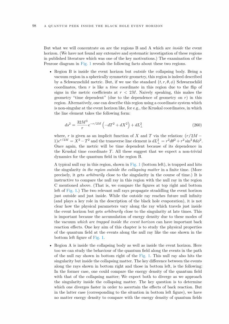
98 a quantum peek inside the black hole event horizon

But what we will concentrate on are the regions B and A which are inside the eventhorizon. (We have not found any extensive and systematic investigation of these regionsin published literature which was one of the key motivations.) The examination of thePenrose diagram in Fig. 1 reveals the following facts about these two regions.

• Region B is inside the event horizon but outside the collapsing body. Being avacuum region in a spherically symmetric geometry, this region is indeed describedby a Schwarzschild metric. But, if we use the standard (t, r, θ,φ) Schwarzschildcoordinates, then r is like a time coordinate in this region due to the flip ofsigns in the metric coefficients at r < 2M . Naively speaking, this makes thegeometry “time dependent” (due to the dependence of geometry on r) in thisregion. Alternatively, one can describe this region using a coordinate system whichis non-singular at the event horizon like, for e.g., the Kruskal coordinates, in whichthe line element takes the following form:

ds2 =32M3

re−r/2M

(−dT 2 + dX2

)+ dL2

⊥ (260)

where, r is given as an implicit function of X and T via the relation: (r/2M −1)er/2M = X2−T 2 and the transverse line element is dL2

⊥ = r2dθ2 + r2 sin2 θdφ2.Once again, the metric will be time dependent because of its dependence inthe Kruskal time coordinate T . All these suggest that we expect a non-trivialdynamics for the quantum field in the region B.

A typical null ray in this region, shown in Fig. 1 (bottom left), is trapped and hitsthe singularity in the region outside the collapsing matter in a finite time. (Moreprecisely, it gets arbitrarily close to the singularity in the course of time.) It isinstructive to compare the null ray in this region with the null ray in the regionC mentioned above. (That is, we compare the figures at top right and bottomleft of Fig. 1.) The two relevant null rays propagate straddling the event horizonjust outside and just inside. While the outside ray reaches future null infinity(and plays a key role in the description of the black hole evaporation), it is notclear how the physical parameters vary along the ray which travels just insidethe event horizon but gets arbitrarily close to the singularity at late times. Thisis important because the accumulation of energy density due to these modes ofthe vacuum which are trapped inside the event horizon can have important backreaction effects. One key aim of this chapter is to study the physical propertiesof the quantum field at the events along the null ray like the one shown in thebottom left figure of Fig. 1.

• Region A is inside the collapsing body as well as inside the event horizon. Heretoo we can study the behaviour of the quantum field along the events in the pathof the null ray shown in bottom right of the Fig. 1. This null ray also hits thesingularity but inside the collapsing matter. The key difference between the eventsalong the rays shown in bottom right and those in bottom left, is the following:In the former case, one could compare the energy density of the quantum fieldwith that of the collapsing matter; We expect both to diverge as we approachthe singularity inside the collapsing matter. The key question is to determinewhich one diverges faster in order to ascertain the effects of back reaction. Butin the latter case (corresponding to the situation in bottom left figure), we haveno matter energy density to compare with the energy density of quantum fields

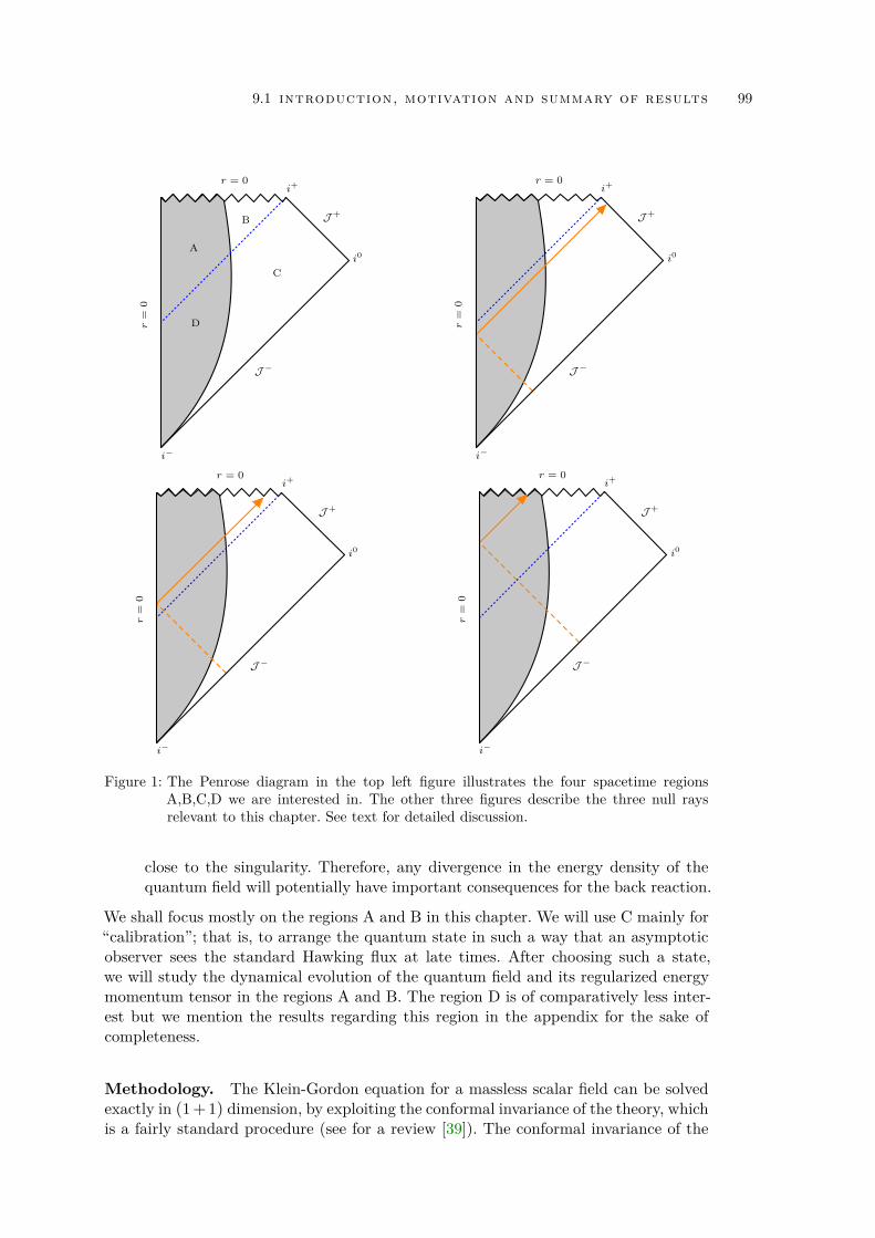
9.1 introduction, motivation and summary of results 99

i

i0

i+r = 0

J

J +

r=

0

A

B

C

D

i

i0

i+r = 0

J

J +

r=

0

i

i0

i+r = 0

J

J +

r=

0

i

i0

i+r = 0

J

J +

r=

0

Figure 1: The Penrose diagram in the top left figure illustrates the four spacetime regionsA,B,C,D we are interested in. The other three figures describe the three null raysrelevant to this chapter. See text for detailed discussion.

close to the singularity. Therefore, any divergence in the energy density of thequantum field will potentially have important consequences for the back reaction.

We shall focus mostly on the regions A and B in this chapter. We will use C mainly for“calibration”; that is, to arrange the quantum state in such a way that an asymptoticobserver sees the standard Hawking flux at late times. After choosing such a state,we will study the dynamical evolution of the quantum field and its regularized energymomentum tensor in the regions A and B. The region D is of comparatively less inter-est but we mention the results regarding this region in the appendix for the sake ofcompleteness.

Methodology. The Klein-Gordon equation for a massless scalar field can be solvedexactly in (1+ 1) dimension, by exploiting the conformal invariance of the theory, whichis a fairly standard procedure (see for a review [39]). The conformal invariance of the

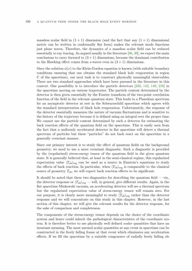
100 a quantum peek inside the black hole event horizon

massless scalar field in (1 + 1) dimension (and the fact that any (1 + 1) dimensionalmetric can be written in conformally flat form) makes the relevant mode functionsjust plane waves. Therefore, the dynamics of a massless scalar field can be reducedessentially to ray tracing. As argued usually in the literature [86, 39], we expect the mainconclusions to carry forward to (3+ 1) dimensions, because the dominant contributionto the Hawking effect comes from s-waves even in (3 + 1) dimensions.

Once the solution φ(x) to the Klein-Gordon equation is known (with suitable boundaryconditions ensuring that one obtains the standard black hole evaporation in regionC of the spacetime), our next task is to construct physically meaningful observables.There are two standard approaches which have been pursued in the literature in thiscontext. One possibility is to introduce the particle detectors [233, 142, 149, 216] inthe spacetime moving on various trajectories. The particle content determined by thedetector is then given essentially by the Fourier transform of the two-point correlationfunction of the field in the relevant quantum state. This leads to a Planckian spectrumfor an asymptotic detector at rest in the Schwarzschild spacetime which agrees withthe standard interpretation of black hole evaporation. Unfortunately, the response ofthe detector essentially measures the nature of vacuum fluctuations and is sensitive tothe history of the trajectory because it is defined using an integral over the proper time.We cannot use the particle content determined by such a detector for estimating theback reaction effects of the quantum field on the spacetime. This is easily seen fromthe fact that a uniformly accelerated detector in flat spacetime will detect a thermalspectrum of particles but these “particles” do not back react on the spacetime in agenerally covariant manner.

Since our primary interest is to study the effect of quantum fields on the backgroundgeometry, we need to use a more covariant diagnostic. Such a diagnostic is providedby the (regularised) stress-energy tensor of the quantum field in the given quantumstate. It is generally believed that, at least in the semi-classical regime, this regularizedexpectation value 〈Tab〉reg can be used as a source in Einstein’s equations to studythe effects of back reaction. In particular, when 〈Tab〉reg is comparable to the classicalsource of geometry Tab, we will expect back reaction effects to be significant.

It should be noted that these two diagnostics for describing the quantum field — viz.,the detector response or 〈Tab〉reg — will, in general, give different results. Again, in theflat spacetime Minkowski vacuum, an accelerating detector will see a thermal spectrumbut the regularized expectation value of stress-energy tensor will remain zero. Forour purpose, it is clearly more meaningful to study 〈Tab〉reg rather than the detectorresponse and we will concentrate on this study in this chapter. However, in the lastsection of this chapter, we will give the relevant results for the detector response, forthe sake of comparison and completeness.

The components of the stress-energy tensor depends on the choice of the coordinatesystem and hence could inherit the pathological characteristics of the coordinate sys-tem. It is therefore better to use physically well defined scalar quantities that have aninvariant meaning. The most natural scalar quantities at any event in spacetime can beconstructed in the freely falling frame at that event which eliminates any accelerationeffects. If we fill the spacetime by a suitable congruence of radially freely falling ob-

9.1 introduction, motivation and summary of results 101

r = 0

VU

12

to∞

Collapsing body

Figure 2: The collapse scenario in the Kruskal coordinates indicating the r = 0 and r = εsurfaces. Of the two null rays which are marked, the ray 1 reaches arbitrarily closeto the singularity in finite time while the ray 2 propagates to asymptotic infinity atlate times. We will be interested in the energy density of the quantum field alongthe events in the path of ray 1, while ray 2 will be used for calibration. See text fordetailed discussion.

servers with four-velocity ua, then we can construct [87, 88, 89, 237, 238, 239, 196] twouseful scalar quantities, at any event in spacetime, by the following definition:

U = 〈Tab〉uaub; F = −〈Tab〉uanb (261)

Here na is the normal in the radial direction (such that uana = 0), U is the energydensity and F is the flux at that event as measured by a freely falling observer.

As we said before, the most natural choice for ua is the four-velocity of the freelyfalling observers which are free of the acceleration effects. Further, we can fill the entirespacetime with the freely falling observers, which allows a fairly uniform descriptionof all the regions of the spacetime. But, in principle, one can also define the scalars inEq. (261) corresponding to any observer with a given four-velocity ua and correspondingna. This is relevant in regions C and D of the spacetime where one can also introducestatic observers and compute the energy density and flux as measured by them. Beforeproceeding further one needs to clarify couple of issues related to this approach. First,note that the r = 0 singularity is a mathematically ill-defined event. Even though in theKruskal coordinates in Fig. 2 (both in (1+1) dimension and in (3+ 1) dimension) it isdrawn as a hyperbola, with distinct (T ,X) coordinates along it, related by T 2−X2 =1 one needs to be careful while dealing with the mathematically ill-defined natureof this event. (For example, consider the two events on which the two null rays inbottom-left and bottom-right figures of Fig. 1 hit the singularity. One could worrywhether these two events are physically distinct.) This is particularly true in the (3+ 1)dimension in which the angular part vanishes at r = 0. To keep our discussion physicallyunambiguous, we will work throughout this chapter with a surface infinitesimally closeto r = 0 but non-singular. Since r 6= 0 on this surface (see Fig. 2) any two separatepoints on it are indeed distinct. Thus by working on a r = ε surface, with arbitrarysmall ε these issues can be avoided.

Second, the divergences in the densities in the (3 + 1) dimension can sometimes bespurious because the volume factor can become arbitrarily small. So one can have a

102 a quantum peek inside the black hole event horizon

situation in which U diverges but U√hd3x remains finite just because of geometrical

considerations. So before we declare the energy density to be divergent in (3 + 1)dimension we need to ensure that the total energy contained inside a small volumeitself diverges, rather than just the energy density. This requires us to define a 3-volumeelement inside the event horizon. (One cannot, of course, use 4πr2dr because insidethe event horizon, r = constant surfaces are spacelike.) When we use a freely-fallingobserver with the four-velocity ua to define U , the appropriate 3-volume measure to useis the one corresponding to the same observer in the synchronous coordinates. Using thismeasure and integrating U

√hd3x over a small volume around the singularity, we can

determine the proper nature of divergence near r = 0. We will show later that the energydensity U diverges in both regions A and B in (1+1) spacetime dimensions. However in(3 + 1) dimension the divergence in region A is compensated by the shrinking volumemeasure (thereby making the energy inside a small region around the singularity finite),while the divergence in region B persists, even though it is milder (being only ε−4/3

compared to ε−2 in the (1+1) dimensions).

We will work with the Oppenheimer-Snyder model [170, 235, 210, 53, 205, 71, 231],which corresponds to collapsing dust (matter with zero pressure) that forms a blackhole. In this case, the spacetime inside the collapsing matter is described by the closedFriedmann metric. To compute the (regularised) stress-energy tensor of the field ina particular quantum state, we use the tools of the standard conformal field theorytechniques. (We expect the results to map to the s-wave sector of the scalar fieldin the collapsing background in (3 + 1) case which is the usual assumption made inliterature; see e.g., [86, 39]) This essentially implies that at any point of the spacetime,we have ingoing and outgoing (spherical) waves and hence the whole manifold can becoordinatized using these null rays. The incoming ray comes directly from J − and theoutgoing ray comes from J − after a reflection from the vertical line in the Penrosediagrams, representing r = 0. As for the vacuum state, we shall work with the naturalin-vacuum that is uniquely defined on J −. The relation of this state with the Unruhvacuum and its effects in the region C for the case of thin null shell collapse have beendiscussed in the refs. [220, 221, 222] and will not be repeated here.

The plan of this chapter is as follows. We briefly review the matching of the interiorand exterior parts of the spacetime for a collapsing dust ball in Section 9.2 and thenintroduce the double null coordinate spanning all of the spacetime. In Section 9.3,we consider the scalar field on this background and compute the components of theregularised stress-energy tensor for same. Subsequently, we compute the energy densityand fluxes for various cases in Section 9.4. Introducing the radially infalling observers,we study the behaviour of the invariant observables U and F along the three null raysmentioned earlier in Section 9.5. Lastly, for the sake of completeness, we discuss theresults regarding the detector response in terms of the effective temperature in Section9.6. The last section contains the concluding remarks.

9.2 the gravitational collapse geometry

In this section, we briefly review the junction conditions for matching the interiorFriedmann universe to the exterior Schwarzschild spacetime.We will then introduce auseful global coordinate system (which we call the double null coordinates) and express

9.2 the gravitational collapse geometry 103

both the interior and exterior coordinates in terms of this double null coordinates in aconformally flat form, in the (1+ 1) sector of the spacetime. This allows us to determinethe conformal factor of the metric from which we can calculate the regularised stress-energy tensor.

9.2.1 Junction Conditions

We consider the collapse of a spherical region filled with pressure-free dust in the(3+ 1) spacetime dimensions. The inside region of the dust sphere is homogeneous andisotropic and the metric interior to the dust will be a closed (k = 1) Friedmann modelwith the line element

ds2int = −dτ2 + a2(τ )dχ2 + a2(τ )dL2

⊥ (262)

with τ denoting proper time of the dust particles, comoving with xµ = constant anddL2⊥ = sin2 χdΩ2. A more convenient form for the line element can be obtained by

transforming the proper time to conformal time η via the relation:

η =∫

dτ

a(τ )(263)

in terms of which the interior metric reduces to the following form:

ds2int = a2(η)

(−dη2 + dχ2 + dL2

⊥

). (264)

The Einstein’s equations for the interior Friedmann universe filled with dust can besolved in a parametric form leading to the results:

a(η) =12amax (1 + cos η) (265)

τ (η) =12amax (η+ sin η) (266)

In these conformal coordinates the surface of the dust sphere is taken to be locatedat some value χ = χ0 and the collapse starts at η = τ = 0 and ends at η = π, τ =(π/2)amax. The total energy contained within the dust sphere is constant and can bedetermined in terms of the quantity amax as:

ρa3 = constant = 38πamax (267)

The exterior region, which is spherically symmetric and empty, is described by Schwarzschildmetric but in a different set of coordinates. The spherical symmetry both inside andoutside suggests that the angular coordinates for both the metric can be taken to beidentical. Hence the outside line element has the following expression (we shall use theunits with 2M = 1 henceforth):

ds2ext = −

(1− 1

r

)dt2 +

(1− 1

r

)−1dr2 + dL2

⊥ (268)

104 a quantum peek inside the black hole event horizon

where we have dL2⊥ = r2dΩ2. The above line element can also be written in terms of

outgoing Eddington-Finkelstein coordinates v = t+ r∗, with r∗ = r+ ln (r− 1), suchthat the line element reduces to

ds2ext = −

(1− 1

r

)dv2 + 2dvdr+ dL2

⊥ (269)

In the outside coordinates the surface of the collapsing matter is characterized byr = r(τ ) and t = t(τ ), where, r and t are the Schwarzschild coordinates with τ beingthe internal time coordinate. The above surface is also determined by χ = χ0. Thereforethe connecting equation for radial coordinate is [232, 205]:

r(η) = a(η) sinχ0 =12amax sinχ0 (1 + cos η) (270)

Next we need to solve for the time coordinate, which is obtained by solving the followingdifferential equation:(

1− 1r

)dt

dτ= constant (271)

Matching the extrinsic curvature on both sides of the surface of the dust sphere wecan fix the constant to be cosχ0. This leads to the following differential equation forSchwarzschild time as:

dt

dη= amax cosχ0 cos2 η

2 +amax cosχ0 cos2 η

2amax sinχ0 cos2 η

2 − 1 (272)

Thus the time coordinate can be obtained from the above equation as:

t(η) =

(1 + amax sinχ0

2

)cotχ0

η+ amax cosχ0 sin η2 cos η2

+ ln∣∣∣∣∣sin2 η

2 − cos2 η2 + amax sinχ0 cos2 η

2 + 2 cotχ0 sin η2 cos η2(

amax sinχ0 cos2 η2 − 1

) ∣∣∣∣∣ (273)

The time corresponding to horizon crossing of the collapsing surface can be obtainedby setting r = 1, which leads to, ηH = π − 2χ0. Note that as η → ηH , t(η) diverges;thus, for an outside observer, the surface of the imploding matter takes infinite timeto reach the event horizon. The amax and χ0 are not independent, since mass of theimploding dust ball is:

M =4π3 ρr3 =

4π3 ρa3 sin3 χ0 =

12amax sin3 χ0 (274)

Thus with 2M = 1 we are left with the condition amax sin3 χ0 = 1. With these con-ditions we find the connection between the Eddington-Finkelstein coordinate v in theexterior region to that of interior region to be:

v(η) =

cotχ0

(1 + amax sinχ0

2

)η+ amax sinχ0

[cos η2 + cotχ0 sin η2

]cos η2

+ 2 ln∣∣∣∣sin η2 + cotχ0 cos η2

∣∣∣∣ (275)

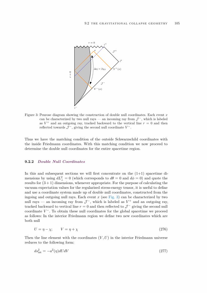
9.2 the gravitational collapse geometry 105

i

i0

i+r = 0

J

J +

r=

0

x

V +(x)

V (x)

= 20

Figure 3: Penrose diagram showing the construction of double null coordinates. Each event xcan be characterized by two null rays — an incoming ray from J−, which is labeledas V + and an outgoing ray, tracked backward to the vertical line r = 0 and thenreflected towards J−, giving the second null coordinate V −.

Thus we have the matching condition of the outside Schwarzschild coordinates withthe inside Friedmann coordinates. With this matching condition we now proceed todetermine the double null coordinates for the entire spacetime region.

9.2.2 Double Null Coordinates

In this and subsequent sections we will first concentrate on the (1+1) spacetime di-mensions by using dL2

⊥ = 0 (which corresponds to dθ = 0 and dφ = 0) and quote theresults for (3+ 1) dimensions, whenever appropriate. For the purpose of calculating thevacuum expectation values for the regularised stress-energy tensor, it is useful to defineand use a coordinate system made up of double null coordinates, constructed from theingoing and outgoing null rays. Each event x (see Fig. 3) can be characterized by twonull rays — an incoming ray from J −, which is labeled as V + and an outgoing ray,tracked backward to vertical line r = 0 and then reflected to J − giving the second nullcoordinate V −. To obtain these null coordinates for the global spacetime we proceedas follows: In the interior Friedmann region we define two new coordinates which areboth null

U = η− χ; V = η+ χ (276)

Then the line element with the coordinates (V ,U) in the interior Friedmann universereduces to the following form:

ds2int = −a2(η)dUdV (277)

106 a quantum peek inside the black hole event horizon

In order to describe the exterior structure we define ingoing and outgoing Eddington-Finkelstein coordinates v and u both being null. The exterior line element reducesto:

ds2ext = −

(1− 1

r

)dudv (278)

in the null coordinates (v,u). Then we can define the double null coordinates V + andV − through the following relations related to the interior Friedmann universe as:

V + = A(V − χ0) (279)V − = A(U − χ0) (280)

where we have introduced the function A(x) for future convenience:

A(x) ≡

cotχ0

(1 + amax sinχ0

2

)x+ 2 ln

∣∣∣∣sin x2 + cotχ0 cos x2

∣∣∣∣+ amax sinχ0

[cos x2 + cotχ0 sin x2

]cos x2 (281)

which connect the interior coordinates (U ,V ) to the global double null coordinates(V +,V −).

From the construction it is easy to verify the following results. The surface r = 0, whichin the FRW universe, has equation χ = 0 or equivalently (from Eq. (276)) U = V . Thusfrom Eq. (279) and Eq. (280) it is evident that V + = V −. Thus the two null coordinatescoincide at r = 0. Also these null coordinates should be continuous on the surface. Thenusing the fact that V = η+χ0 on the surface of the star from Eq. (279) we get, V + = v,which it should. For χ 6= 0, the value of V + and V − are never equal for all η. Thisimplies that even though the singularity forms at η = π, in the double null coordinates itis ‘spread out’. The value of V − for the outer surface of the star to reach the singularityis obtained by using U = π − χ0, leading to, V − = A(π − 2χ0). By construction thismust be equal to V + of the point, where the ray enters the dust sphere, which is A(η).This helps us to identify, the time at which that particular null ray has entered thesphere as π− 2χ0. This, in turn, fixes the surface of the star completely. Note that thisis just a corollary of a more general result: The null rays entering the sphere, gettingreflected at r = 0 and exiting the sphere satisfy the relation, dη = dχ. Thus the raystarts at χ = χ0, then goes to χ = 0, again comes out at χ = χ0. The difference in thecoordinate values for η between the point of entering and exit of the ray correspondsto ∆η = 2χ0 (see Fig. 3). Hence in the above situation, the final value of η is π, andthe entry value of η has to be π− 2χ0, leading back to the previous result.

Another set of relations connecting exterior coordinates (u, v) to the global null coor-dinates (V +,V −) are given by:

v = V + (282)u = B(U + χ0) = A(U + χ0)− amax sinχ0 (1 + cos(U + χ0))

− 2 ln∣∣∣∣amax sinχ0 cos2

(U + χ0

2

)− 1

∣∣∣∣ (283)

9.3 regularised stress-energy tensor 107

Thus the interior and exterior line elements can be written in the double null coordinatesystem (V +,V −) in the following manner:

ds2int = −a2

(U + V

2

) 1dAdU

dAdV

dV +dV − (284)

ds2ext = −

(1− 1

r

)dB/dUdA/dU

dV +dV − (285)

Hence this double null coordinate covers the full spacetime and brings the (1+ 1) sectorof the spacetime to the conformally flat form. This is especially suited to evaluate thevacuum expectation value of the regularised stress-energy tensor, which is our nexttask.

9.3 regularised stress-energy tensor

We consider a minimally coupled, massless scalar field on the background geometrydescribed by the line elements in Eq. (284) and Eq. (285). In two dimension the dy-namics of the geometry is encoded in the conformal factor which allows us to obtainthe vacuum expectation value of the energy momentum tensor for the scalar field. Forthis we follow the standard procedure [71, 39] and use the following expressions givenin terms of the conformal factor:

〈T++〉 =1

12π

[12∂2+C

C− 3

4

(∂+C

C

)2](286)

〈T−−〉 =1

12π

[12∂2−C

C− 3

4

(∂−C

C

)2](287)

〈T+−〉 =1

24π

[∂+∂−C

C− ∂+C

C

∂−C

C

](288)

In the above expressions we have introduced a short hand notation: the symbol ±stands for V ± respectively. The detailed computation and the explicit expression forthe regularised stress-energy tensor, using these relations is given in the AppendixF.1.

9.4 energy density and flux observed by different observers

We shall now compute the energy density and flux at different events in the spacetimeusing the regularised stress tensor. As we described earlier our primary interest is inthe regions B and A inside the event horizon where no static observers can exist. Inthese regions, we will study the energy density and the flux in the freely-falling frame.But before we do that, it is useful to consider the region C and see how the standardresults are reproduced. In this region C (unlike in A and B) we can introduce bothstatic and freely falling observers and study the flux and energy density as measuredby both kinds of observers.

108 a quantum peek inside the black hole event horizon

9.4.1 Static Observers in region C

We will start with the energy density and flux as measured by the static observersin region C. This will verify our procedure by leading to the standard result of theHawking radiation with the Tolman redshifted temperature.

A static observer stays outside the event horizon at some fixed radius r > 1. Since theobserver is not following geodesic he/she has to accelerate (by firing rockets) so as toremain stationary at that radius. The velocity components for this static observer isgiven by:

V + =

√r

r− 1 (289)

V − =

√r

r− 1

cotχ0 − tan(U+χ0

2

)cotχ0 + tan

(U−χ0

2

) cos2

(U−χ0

2

)cos2

(U+χ0

2

) (290)

for a fixed r. The outward normal, determined from the condition naV a = 0, has thefollowing components:

n+ = V +; n− = −V − (291)

Thus the energy density and flux can be computed using Eq. (261) for the static tra-jectories as a function of V +. For static observers V + acts as the proper time alongtheir trajectories and we plot both the energy density and flux as a function of V +

in Fig. 4. From this figure we see that both energy density and flux shows similarbehaviour at large radii. Both of them start from small positive values and finally satu-rate at the standard thermal spectrum values with the Tolman redshifted value for thetemperature.

The key results we want to verify for the static observers are, of course, the late timeenergy density and flux. The late time limit corresponds to U → π− 3χ0, under whichboth the energy density and the flux lead to the following expressions:

U =πT 2

H

12

(1− 2

r4

)(r

r− 1

)(292a)

F =πT 2

H

12r

r− 1 (292b)

We see that, in the asymptotic limit, r → ∞ (corresponding to a static observer at alarge distance) above expressions reduce to the standard Hawking energy density andflux. The redshift factor, as is well-known, diverges as the horizon r = 1 is approached.From Eq. (292a) it is evident that in the near horizon limit the energy density reachesa maximum and then decreases with decreasing r, eventually becoming negative. Thus,even in the Oppenheimer-Snyder dust model there is a region of negative energy densityjust outside the black hole horizon, just as in the case of a null shell collapse noticedearlier e.g., in [221]. However the flux is always positive and diverges at the horizon.

9.4 energy density and flux observed by different observers 109

r=50 rs

r=30 rs

r=20 rs

0 50 100 150 200 2500.0

0.2

0.4

0.6

0.8

1.0

1.2

V+

EnergyDensity r=50 rs

r=30 rs

r=20 rs

0 50 100 150 200 2500.0

0.2

0.4

0.6

0.8

1.0

1.2

V+

Flux

Figure 4: Variation of the energy density and the flux as observed by a static observer as afunction of the proper time. The first figure shows the variation of the energy densitywith proper time V +. All the static observers at different radii will ultimately observethe standard result for the Hawking radiation with the temperature modified by theTolman redshift factor. (Note that while plotting the graphs we have normalizedthem to their values at infinity, i.e., πT 2

H/12 for convenience.) The same situation isdepicted in the second figure for the flux. Both start with a small value and then riserapidly, ultimately saturating at the appropriate values for the Hawking radiationwith the redshifted temperature.

9.4.2 Radially In-falling Observers

Having reproduced the standard results in region C we now turn our attention to thephenomena inside the event horizon. Since there can be no static observers in thisregion, it is best to study these effects in the freely falling frame of the radially ingoingobserver. To provide the complete picture and to maintain continuity, we will study theresults for the freely falling observers in the entire spacetime. This can be done fromtwo different perspectives:

(1) We can compute the energy density and flux on the events along the trajectory ofa given freely falling observer. This has a clear physical meaning of what such a freelyfalling observer will see, as she plunges into the singularity.

(2) We can examine the energy density and flux on the events along specific null rayswe described in Section 9.1 (see Fig. 1). This will tell us how the energy density andflux behaves on a selected set of events in the spacetime which are physically well-motivated.

In this section, we shall present the results based on the approach (1), viz. along thetrajectories of the observers. We shall describe the behaviour of the energy density andflux on the events along the specific null rays in Section 9.5.

Since part of the spacetime is covered by the collapsing dust ball, there exist two typesof radially in-falling observers. The first set of observers are (i) those who are comovingwith the dust sphere and remain inside the collapsing matter, while the second set ofobservers are (ii) those who are always outside the dust sphere. The first set of observerswho stay inside the dust sphere ultimately reach the singularity in a finite proper time.These observers are in a Friedmann universe. The observers in a region outside thecollapsing matter also hit the singularity in finite time but they live in a Schwarzschild

110 a quantum peek inside the black hole event horizon

geometry. Thus these two observers are geometrically distinct even though both ofthem hit the singularity in a finite proper time. We will now consider these two sets offreely falling observers and use them to probe the regions D, A and B.

9.4.2.1 Radially In-falling Observers: Inside regions D and A

Let us start with the observers who are inside the dust sphere and are comoving withit. All these observers start at η = 0 when the dust sphere starts to collapse and reachη = π in a finite proper time. The trajectory of these observers are characterized bythe conformal time η. For such an observer comoving with the dust sphere, the fourvelocity is given by:

ua =1√

2a (η)

(dA

dV, dAdU

)(293)

ua = −a√2

( 1dA/dV

, 1dA/dU

)(294)

and the unit normal has the following expression:

na =a√2

(1dAdV

,− 1dAdU

)(295)

na =1√2a

(dA

dV,−dA

dU

)(296)

The comoving observer is characterized by the value of χ which remains fixed through-out the trajectory (taken as χ) and hits the singularity as η varies from 0 to π. Thevariation of energy density for the comoving observer with the proper time η alongthe trajectory is shown in Fig. 5. We note that the energy density for the outermostobserver at χ = χ0 remains positive and diverges as η → π. While the energy densityas measured by other observers remain finite while reaching a maximum near η = πand then becomes negative. Finally the energy densities for all the observers diverge inthe η → π limit. This result is shown in Fig. 5.

The energy density diverges as the observer hits the singularity. The ratio of the energydensity measured by the observer to that of the energy density of the collapsing matteralso diverges. This divergence can be obtained from the leading order behaviour of Uand ρ near r = 0, which can be represented, for (1+1) spacetime dimensions, as: (seeEq. (638) in the Appendix F.2.2)

U (1) = −κ2amax6πa3 ; ρ(1) =

amax sin2 χ02a ; U (1)

ρ(1)∝ 1a2 (297)

where superscript (1) denote the values of respective quantities in (1+1) spacetime di-mensions. Thus, close to the singularity, the energy density of the scalar field dominatesover that of the dust sphere.

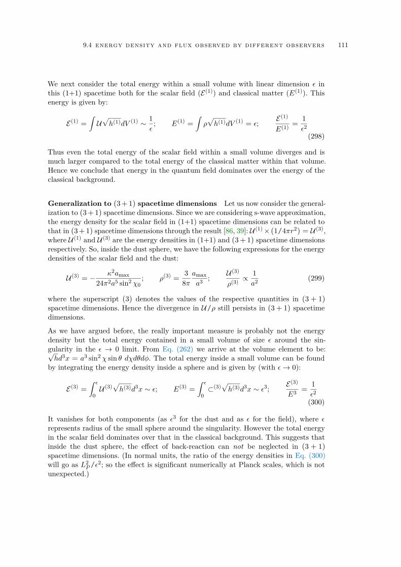
9.4 energy density and flux observed by different observers 111

We next consider the total energy within a small volume with linear dimension ε inthis (1+1) spacetime both for the scalar field (E (1)) and classical matter (E(1)). Thisenergy is given by:

E (1) =∫U√h(1)dV (1) ∼ 1

ε; E(1) =

∫ρ√h(1)dV (1) = ε; E (1)

E(1) =1ε2

(298)

Thus even the total energy of the scalar field within a small volume diverges and ismuch larger compared to the total energy of the classical matter within that volume.Hence we conclude that energy in the quantum field dominates over the energy of theclassical background.

Generalization to (3+ 1) spacetime dimensions Let us now consider the general-ization to (3+ 1) spacetime dimensions. Since we are considering s-wave approximation,the energy density for the scalar field in (1+1) spacetime dimensions can be related tothat in (3+ 1) spacetime dimensions through the result [86, 39]: U (1)× (1/4πr2) = U (3),where U (1) and U (3) are the energy densities in (1+1) and (3+ 1) spacetime dimensionsrespectively. So, inside the dust sphere, we have the following expressions for the energydensities of the scalar field and the dust:

U (3) = − κ2amax24π2a5 sin2 χ0

; ρ(3) =3

8πamaxa3 ; U (3)

ρ(3)∝ 1a2 (299)

where the superscript (3) denotes the values of the respective quantities in (3 + 1)spacetime dimensions. Hence the divergence in U/ρ still persists in (3 + 1) spacetimedimensions.

As we have argued before, the really important measure is probably not the energydensity but the total energy contained in a small volume of size ε around the sin-gularity in the ε → 0 limit. From Eq. (262) we arrive at the volume element to be:√hd3x = a3 sin2 χ sin θ dχdθdφ. The total energy inside a small volume can be found

by integrating the energy density inside a sphere and is given by (with ε→ 0):

E (3) =∫ ε

0U (3)

√h(3)d3x ∼ ε; E(3) =

∫ ε

0⊂(3)

√h(3)d3x ∼ ε3; E (3)

E3 =1ε2

(300)

It vanishes for both components (as ε3 for the dust and as ε for the field), where εrepresents radius of the small sphere around the singularity. However the total energyin the scalar field dominates over that in the classical background. This suggests thatinside the dust sphere, the effect of back-reaction can not be neglected in (3 + 1)spacetime dimensions. (In normal units, the ratio of the energy densities in Eq. (300)will go as L2

P/ε2; so the effect is significant numerically at Planck scales, which is notunexpected.)

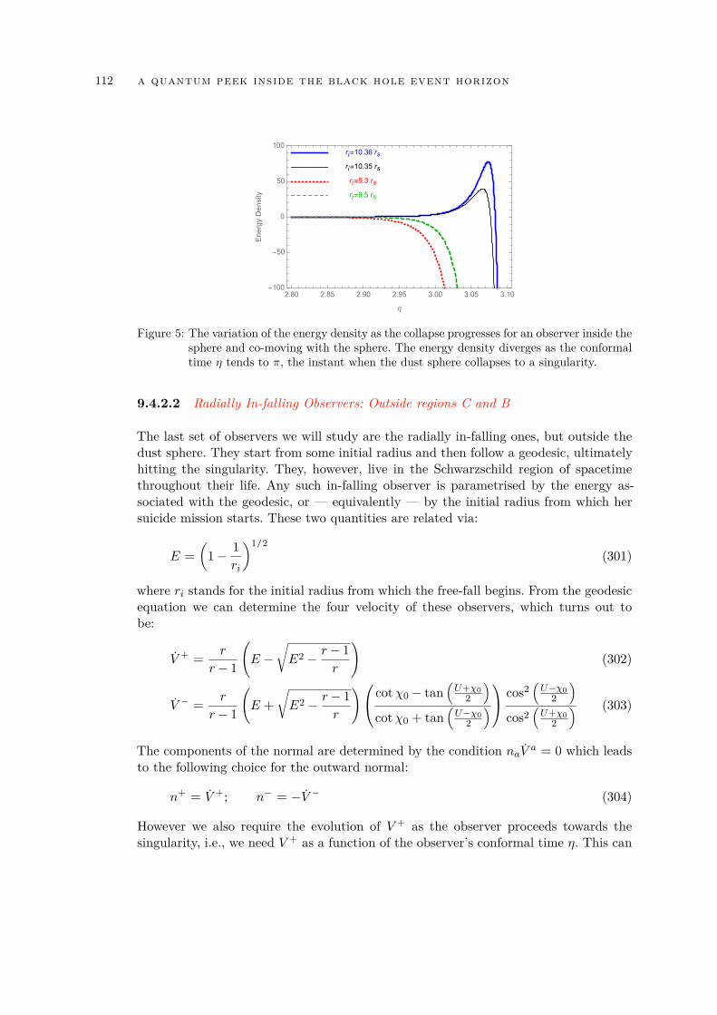
112 a quantum peek inside the black hole event horizon

ri=10.36 rs

ri=10.35 rs

ri=5.3 rs

ri=9.5 rs

2.80 2.85 2.90 2.95 3.00 3.05 3.10-100

-50

0

50

100

η

EnergyDensity

Figure 5: The variation of the energy density as the collapse progresses for an observer inside thesphere and co-moving with the sphere. The energy density diverges as the conformaltime η tends to π, the instant when the dust sphere collapses to a singularity.

9.4.2.2 Radially In-falling Observers: Outside regions C and B

The last set of observers we will study are the radially in-falling ones, but outside thedust sphere. They start from some initial radius and then follow a geodesic, ultimatelyhitting the singularity. They, however, live in the Schwarzschild region of spacetimethroughout their life. Any such in-falling observer is parametrised by the energy as-sociated with the geodesic, or — equivalently — by the initial radius from which hersuicide mission starts. These two quantities are related via:

E =

(1− 1

ri

)1/2(301)

where ri stands for the initial radius from which the free-fall begins. From the geodesicequation we can determine the four velocity of these observers, which turns out tobe:

V + =r

r− 1

(E −

√E2 − r− 1

r

)(302)

V − =r

r− 1

(E +

√E2 − r− 1

r

) cotχ0 − tan(U+χ0

2

)cotχ0 + tan

(U−χ0

2

) cos2

(U−χ0

2

)cos2

(U+χ0

2

) (303)

The components of the normal are determined by the condition naV a = 0 which leadsto the following choice for the outward normal:

n+ = V +; n− = −V − (304)

However we also require the evolution of V + as the observer proceeds towards thesingularity, i.e., we need V + as a function of the observer’s conformal time η. This can

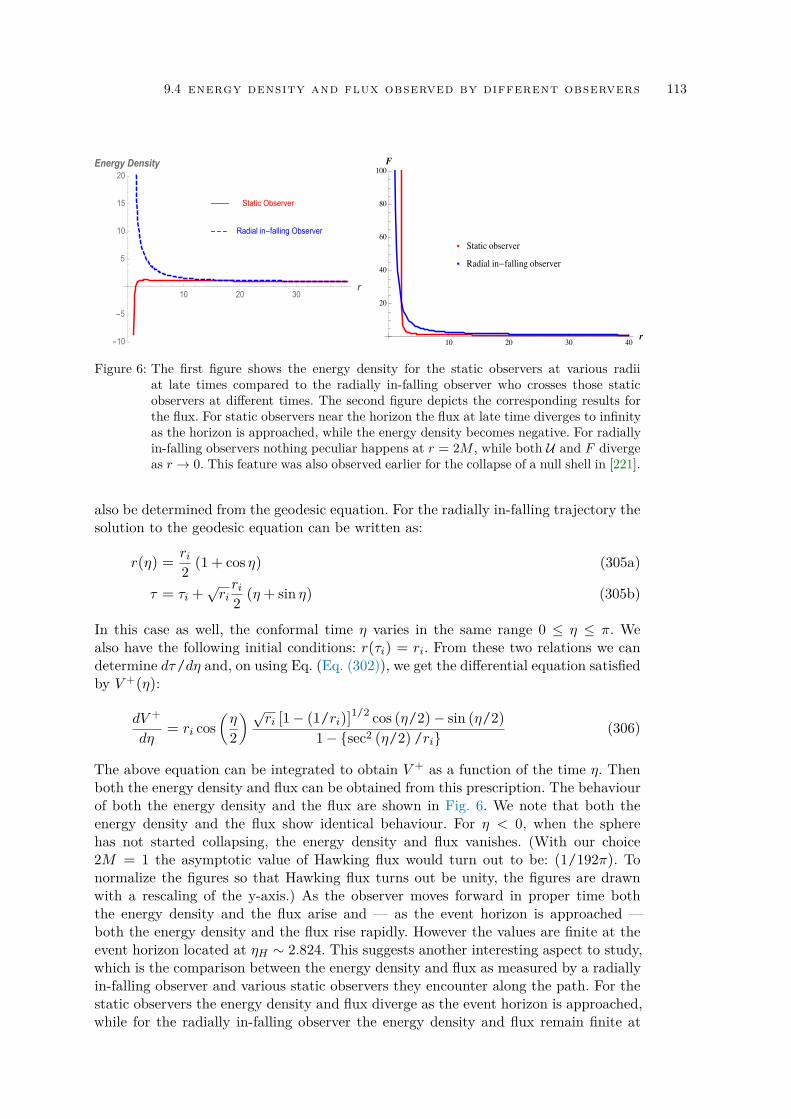
9.4 energy density and flux observed by different observers 113

Static Observer

Radial in-falling Observer

10 20 30r

-10

-5

5

10

15

20Energy Density

Static observer

Radial in-falling observer

10 20 30 40r

20

40

60

80

100F

Figure 6: The first figure shows the energy density for the static observers at various radiiat late times compared to the radially in-falling observer who crosses those staticobservers at different times. The second figure depicts the corresponding results forthe flux. For static observers near the horizon the flux at late time diverges to infinityas the horizon is approached, while the energy density becomes negative. For radiallyin-falling observers nothing peculiar happens at r = 2M , while both U and F divergeas r → 0. This feature was also observed earlier for the collapse of a null shell in [221].

also be determined from the geodesic equation. For the radially in-falling trajectory thesolution to the geodesic equation can be written as:

r(η) =ri2 (1 + cos η) (305a)

τ = τi +√riri2 (η+ sin η) (305b)

In this case as well, the conformal time η varies in the same range 0 ≤ η ≤ π. Wealso have the following initial conditions: r(τi) = ri. From these two relations we candetermine dτ/dη and, on using Eq. (Eq. (302)), we get the differential equation satisfiedby V +(η):

dV +

dη= ri cos

(η

2

) √ri [1− (1/ri)]

1/2 cos (η/2)− sin (η/2)1− sec2 (η/2) /ri

(306)

The above equation can be integrated to obtain V + as a function of the time η. Thenboth the energy density and flux can be obtained from this prescription. The behaviourof both the energy density and the flux are shown in Fig. 6. We note that both theenergy density and the flux show identical behaviour. For η < 0, when the spherehas not started collapsing, the energy density and flux vanishes. (With our choice2M = 1 the asymptotic value of Hawking flux would turn out to be: (1/192π). Tonormalize the figures so that Hawking flux turns out be unity, the figures are drawnwith a rescaling of the y-axis.) As the observer moves forward in proper time boththe energy density and the flux arise and — as the event horizon is approached —both the energy density and the flux rise rapidly. However the values are finite at theevent horizon located at ηH ∼ 2.824. This suggests another interesting aspect to study,which is the comparison between the energy density and flux as measured by a radiallyin-falling observer and various static observers they encounter along the path. For thestatic observers the energy density and flux diverge as the event horizon is approached,while for the radially in-falling observer the energy density and flux remain finite at

114 a quantum peek inside the black hole event horizon

the horizon crossing. We give below the expressions for the energy density and flux asmeasured by these observers at the horizon:

UH = πT 2H

(23 −

148E2 + 2E2

)(307a)

FH = πT 2H

( 148E2 + 2E2

)(307b)

For a radially in-falling observer from infinity we have E = 1, for which the horizoncrossing energy density and flux becomes UH ∼ 32U∞ and FH ∼ 24F∞. (Note thatthese results were obtained earlier in the context of a null collapse in [221].)

However the energy density and flux finally diverge as the singularity is approached. Thebehaviour of the energy density and its integral over a small volume has the followingexpressions near the singularity: (see Eq. (640) in Appendix F.2.3)

U (1) =7κ2

24π1ε3

; E (1) =∫U√h(1)dV (1) ∼ 1

ε2(308)

where superscript (1) denotes the expression of the quantities in the (1+1) spacetimedimensions. Thus both the energy density and the integrated energy diverges as thesingularity is approached. Hence even in region outside the dust sphere the backreactionis important near the singularity.

Generalization to (3+ 1) spacetime dimensions The energy density of the scalarfield, as measured by the radially in-falling observers, in (3 + 1) spacetime dimensionscan be obtained by dividing the (1+1) energy density by 4πr2. (This is a standardprocedure adopted in the literature; see e.g., [86, 39]). This leads to the followingapproximate expression for the energy density near the singularity:

U (3) =7κ2

96π21r5 (309)

This result, at the face of it, shows that the back-reaction effects will be quite significantclose to the singularity even outside the collapsing dust sphere. However, we need toensure that the geometrical factor arising from the shrinking of the spatial volume doesnot over-compensate the divergence. To obtain the proper volume element appropriatefor the radially in-falling observer, let us start with the metric in the synchronouscoordinates for an observer in free-fall, from a large distance:

ds2 = −dτ2 +1rdR2 + r2dΩ2; r =

[32 (R− τ )

]2/3(310)

Thus for a τ = constant surface the volume element turns out to be:√hd3x = r3/2 sin θ dRdθdφ =

32 (R− τ ) sin θdRdθdφ (311)

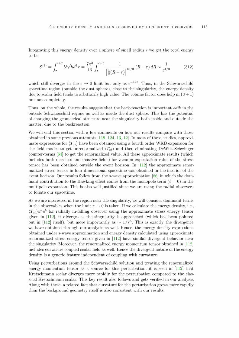
9.4 energy density and flux observed by different observers 115

Integrating this energy density over a sphere of small radius ε we get the total energyto be

E (3) =∫ ε+τ

τU√hd3x =

7κ2

16

∫ ε+τ

τ

1[32 (R− τ )

]10/3 (R− τ ) dR ∼1ε4/3 (312)

which still diverges in the ε → 0 limit but only as ε−4/3. Thus, in the Schwarzschildspacetime region (outside the dust sphere), close to the singularity, the energy densitydue to scalar field tends to arbitrarily high value. The volume factor does help in (3+ 1)but not completely.

Thus, on the whole, the results suggest that the back-reaction is important both in theoutside Schwarzschild regime as well as inside the dust sphere. This has the potentialof changing the geometrical structure near the singularity both inside and outside thematter, due to the backreaction.

We will end this section with a few comments on how our results compare with thoseobtained in some previous attempts [119, 124, 13, 12]. In most of these studies, approxi-mate expressions for 〈Tab〉 have been obtained using a fourth order WKB expansion forthe field modes to get unrenormalized 〈Tab〉 and then eliminating DeWitt-Schwingercounter-terms [64] to get the renormalized value. All these approximate results (whichincludes both massless and massive fields) for vacuum expectation value of the stresstensor has been obtained outside the event horizon. In [112] the approximate renor-malized stress tensor in four-dimensional spacetime was obtained in the interior of theevent horizon. Our results follow from the s-wave approximation [86] in which the dom-inant contribution to the Hawking effect comes from the monopole term (` = 0) in themultipole expansion. This is also well justified since we are using the radial observersto foliate our spacetime.

As we are interested in the region near the singularity, we will consider dominant termsin the observables when the limit r → 0 is taken. If we calculate the energy density, i.e.,〈Tab〉uaub for radially in-falling observer using the approximate stress energy tensorgiven in [112], it diverges as the singularity is approached (which has been pointedout in [112] itself), but more importantly as ∼ 1/r5. This is exactly the divergencewe have obtained through our analysis as well. Hence, the energy density expressionsobtained under s-wave approximation and energy density calculated using approximaterenormalized stress energy tensor given in [112] have similar divergent behavior nearthe singularity. Moreover, the renormalized energy momentum tensor obtained in [112]includes curvature coupled scalar field as well. Hence the divergent nature of the energydensity is a generic feature independent of coupling with curvature.

Using perturbations around the Schwarzschild solution and treating the renormalizedenergy momentum tensor as a source for this perturbation, it is seen in [112] thatKretschmann scalar diverges more rapidly for the perturbation compared to the clas-sical Kretschmann scalar. This key result also follows and gets verified in our analysis.Along with these, a related fact that curvature for the perturbation grows more rapidlythan the background geometry itself is also consistent with our results.

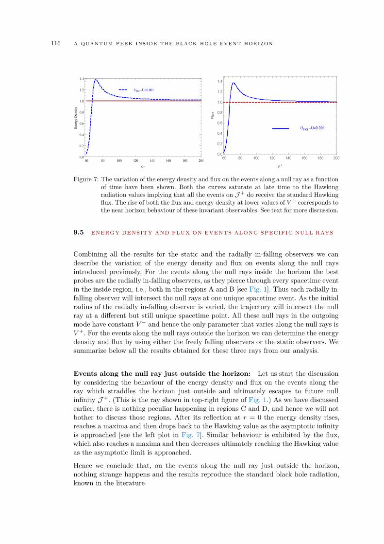
116 a quantum peek inside the black hole event horizon

UHor-U=0.001

60 80 100 120 140 160 180 2000.0

0.2

0.4

0.6

0.8

1.0

1.2

1.4

V+

Energ

yD

ensi

ty

UHor -U=0.001

60 80 100 120 140 160 180 2000.0

0.2

0.4

0.6

0.8

1.0

1.2

1.4

V+

Flux

Figure 7: The variation of the energy density and flux on the events along a null ray as a functionof time have been shown. Both the curves saturate at late time to the Hawkingradiation values implying that all the events on J + do receive the standard Hawkingflux. The rise of both the flux and energy density at lower values of V + corresponds tothe near horizon behaviour of these invariant observables. See text for more discussion.

9.5 energy density and flux on events along specific null rays

Combining all the results for the static and the radially in-falling observers we candescribe the variation of the energy density and flux on events along the null raysintroduced previously. For the events along the null rays inside the horizon the bestprobes are the radially in-falling observers, as they pierce through every spacetime eventin the inside region, i.e., both in the regions A and B [see Fig. 1]. Thus each radially in-falling observer will intersect the null rays at one unique spacetime event. As the initialradius of the radially in-falling observer is varied, the trajectory will intersect the nullray at a different but still unique spacetime point. All these null rays in the outgoingmode have constant V − and hence the only parameter that varies along the null rays isV +. For the events along the null rays outside the horizon we can determine the energydensity and flux by using either the freely falling observers or the static observers. Wesummarize below all the results obtained for these three rays from our analysis.

Events along the null ray just outside the horizon: Let us start the discussionby considering the behaviour of the energy density and flux on the events along theray which straddles the horizon just outside and ultimately escapes to future nullinfinity J +. (This is the ray shown in top-right figure of Fig. 1.) As we have discussedearlier, there is nothing peculiar happening in regions C and D, and hence we will notbother to discuss those regions. After its reflection at r = 0 the energy density rises,reaches a maxima and then drops back to the Hawking value as the asymptotic infinityis approached [see the left plot in Fig. 7]. Similar behaviour is exhibited by the flux,which also reaches a maxima and then decreases ultimately reaching the Hawking valueas the asymptotic limit is approached.

Hence we conclude that, on the events along the null ray just outside the horizon,nothing strange happens and the results reproduce the standard black hole radiation,known in the literature.

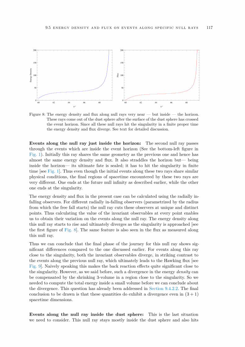
9.5 energy density and flux on events along specific null rays 117

60 62 64 66 680

50

100

150

200

V+

Energ

yD

ensi

ty

60 62 64 66 680

50

100

150

200

V+

Flu

xFigure 8: The energy density and flux along null rays very near — but inside — the horizon.

These rays come out of the dust sphere after the surface of the dust sphere has crossedthe event horizon. Since all these null rays hit the singularity in a finite proper timethe energy density and flux diverge. See text for detailed discussion.

Events along the null ray just inside the horizon: The second null ray passesthrough the events which are inside the event horizon (See the bottom-left figure inFig. 1). Initially this ray shares the same geometry as the previous one and hence hasalmost the same energy density and flux. It also straddles the horizon but— beinginside the horizon— its ultimate fate is sealed; it has to hit the singularity in finitetime [see Fig. 1]. Thus even though the initial events along these two rays share similarphysical conditions, the final regions of spacetime encountered by these two rays arevery different. One ends at the future null infinity as described earlier, while the otherone ends at the singularity.

The energy density and flux in the present case can be calculated using the radially in-falling observers. For different radially in-falling observers (parametrized by the radiusfrom which the free fall starts) the null ray cuts these observers at unique and distinctpoints. Thus calculating the value of the invariant observables at every point enablesus to obtain their variation on the events along the null ray. The energy density alongthis null ray starts to rise and ultimately diverges as the singularity is approached [seethe first figure of Fig. 8]. The same feature is also seen in the flux as measured alongthis null ray.

Thus we can conclude that the final phase of the journey for this null ray shows sig-nificant differences compared to the one discussed earlier. For events along this rayclose to the singularity, both the invariant observables diverge, in striking contrast tothe events along the previous null ray, which ultimately leads to the Hawking flux [seeFig. 9]. Naively speaking this makes the back reaction effects quite significant close tothe singularity. However, as we said before, such a divergence in the energy density canbe compensated by the shrinking 3-volume in a region close to the singularity. So weneeded to compute the total energy inside a small volume before we can conclude aboutthe divergence. This question has already been addressed in Section 9.4.2.2. The finalconclusion to be drawn is that these quantities do exhibit a divergence even in (3 + 1)spacetime dimensions.

Events along the null ray inside the dust sphere: This is the last situationwe need to consider. This null ray stays mostly inside the dust sphere and also hits

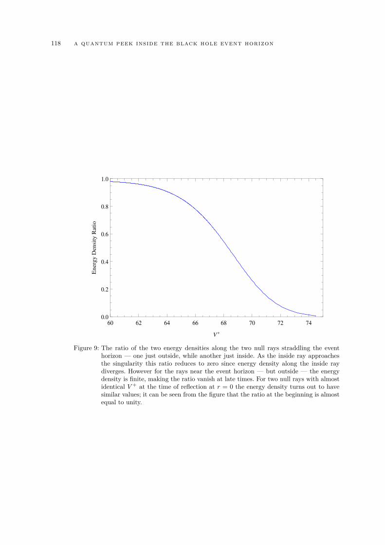
118 a quantum peek inside the black hole event horizon

60 62 64 66 68 70 72 740.0

0.2

0.4

0.6

0.8

1.0

V+

En

erg

yD

en

sity

Rati

o

Figure 9: The ratio of the two energy densities along the two null rays straddling the eventhorizon — one just outside, while another just inside. As the inside ray approachesthe singularity this ratio reduces to zero since energy density along the inside raydiverges. However for the rays near the event horizon — but outside — the energydensity is finite, making the ratio vanish at late times. For two null rays with almostidentical V + at the time of reflection at r = 0 the energy density turns out to havesimilar values; it can be seen from the figure that the ratio at the beginning is almostequal to unity.

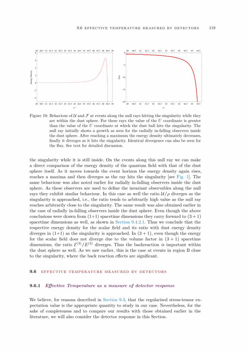
9.6 effective temperature measured by detectors 119

60 60.5 61 61.5 62 62.5 63 63.5 64 64.5 65 65.5 66 67.5 68 68.5 69

-4

-2

0

2

4

6

860 60.5 61 61.5 62 62.5 63 63.5 64 64.5 65 65.5 66 67.5 68 68.5 69

V+

Energ

yD

ensi

ty

60 60.5 61 61.5 62 62.5 63 63.5 64 64.5 65 65.5-20

-15

-10

-5

060 60.5 61 61.5 62 62.5 63 63.5 64 64.5 65 65.5

V+

Flu

xFigure 10: Behaviour of U and F at events along the null rays hitting the singularity while they

are within the dust sphere. For these rays the value of the U coordinate is greaterthan the value of the U coordinate at which the dust ball hits the singularity. Thenull ray initially shows a growth as seen for the radially in-falling observers insidethe dust sphere. After reaching a maximum the energy density ultimately decreases,finally it diverges as it hits the singularity. Identical divergence can also be seen forthe flux. See text for detailed discussion.

the singularity while it is still inside. On the events along this null ray we can makea direct comparison of the energy density of the quantum field with that of the dustsphere itself. As it moves towards the event horizon the energy density again rises,reaches a maxima and then diverges as the ray hits the singularity [see Fig. 1]. Thesame behaviour was also noted earlier for radially in-falling observers inside the dustsphere. As these observers are used to define the invariant observables along the nullrays they exhibit similar behaviour. In this case as well the ratio U/ρ diverges as thesingularity is approached, i.e., the ratio tends to arbitrarily high value as the null rayreaches arbitrarily close to the singularity. The same result was also obtained earlier inthe case of radially in-falling observers inside the dust sphere. Even though the aboveconclusions were drawn from (1+1) spacetime dimensions they carry forward to (3+ 1)spacetime dimensions as well, as shown in Section 9.4.2.1. Thus we conclude that therespective energy density for the scalar field and its ratio with dust energy densitydiverges in (1+1) as the singularity is approached. In (3 + 1), even though the energyfor the scalar field does not diverge due to the volume factor in (3 + 1) spacetimedimensions, the ratio E (3)/E(3) diverges. Thus the backreaction is important withinthe dust sphere as well. As we saw earlier, this is the case at events in region B closeto the singularity, where the back reaction effects are significant.

9.6 effective temperature measured by detectors

9.6.1 Effective Temperature as a measure of detector response

We believe, for reasons described in Section 9.3, that the regularised stress-tensor ex-pectation value is the appropriate quantity to study in our case. Nevertheless, for thesake of completeness and to compare our results with those obtained earlier in theliterature, we will also consider the detector response in this Section.

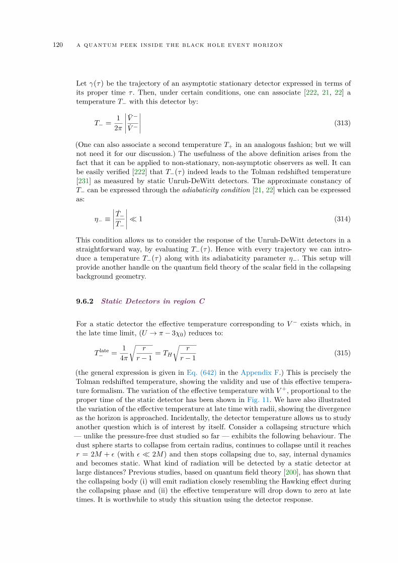
120 a quantum peek inside the black hole event horizon

Let γ(τ ) be the trajectory of an asymptotic stationary detector expressed in terms ofits proper time τ . Then, under certain conditions, one can associate [222, 21, 22] atemperature T− with this detector by:

T− =1

2π

∣∣∣∣∣ V −V −∣∣∣∣∣ (313)

(One can also associate a second temperature T+ in an analogous fashion; but we willnot need it for our discussion.) The usefulness of the above definition arises from thefact that it can be applied to non-stationary, non-asymptotic observers as well. It canbe easily verified [222] that T−(τ ) indeed leads to the Tolman redshifted temperature[231] as measured by static Unruh-DeWitt detectors. The approximate constancy ofT− can be expressed through the adiabaticity condition [21, 22] which can be expressedas:

η− ≡∣∣∣∣∣ T−T−

∣∣∣∣∣ 1 (314)

This condition allows us to consider the response of the Unruh-DeWitt detectors in astraightforward way, by evaluating T−(τ ). Hence with every trajectory we can intro-duce a temperature T−(τ ) along with its adiabaticity parameter η−. This setup willprovide another handle on the quantum field theory of the scalar field in the collapsingbackground geometry.

9.6.2 Static Detectors in region C

For a static detector the effective temperature corresponding to V − exists which, inthe late time limit, (U → π− 3χ0) reduces to:

T late− =

14π

√r

r− 1 = TH

√r

r− 1 (315)

(the general expression is given in Eq. (642) in the Appendix F.) This is precisely theTolman redshifted temperature, showing the validity and use of this effective tempera-ture formalism. The variation of the effective temperature with V +, proportional to theproper time of the static detector has been shown in Fig. 11. We have also illustratedthe variation of the effective temperature at late time with radii, showing the divergenceas the horizon is approached. Incidentally, the detector temperature allows us to studyanother question which is of interest by itself. Consider a collapsing structure which— unlike the pressure-free dust studied so far — exhibits the following behaviour. Thedust sphere starts to collapse from certain radius, continues to collapse until it reachesr = 2M + ε (with ε 2M) and then stops collapsing due to, say, internal dynamicsand becomes static. What kind of radiation will be detected by a static detector atlarge distances? Previous studies, based on quantum field theory [200], has shown thatthe collapsing body (i) will emit radiation closely resembling the Hawking effect duringthe collapsing phase and (ii) the effective temperature will drop down to zero at latetimes. It is worthwhile to study this situation using the detector response.

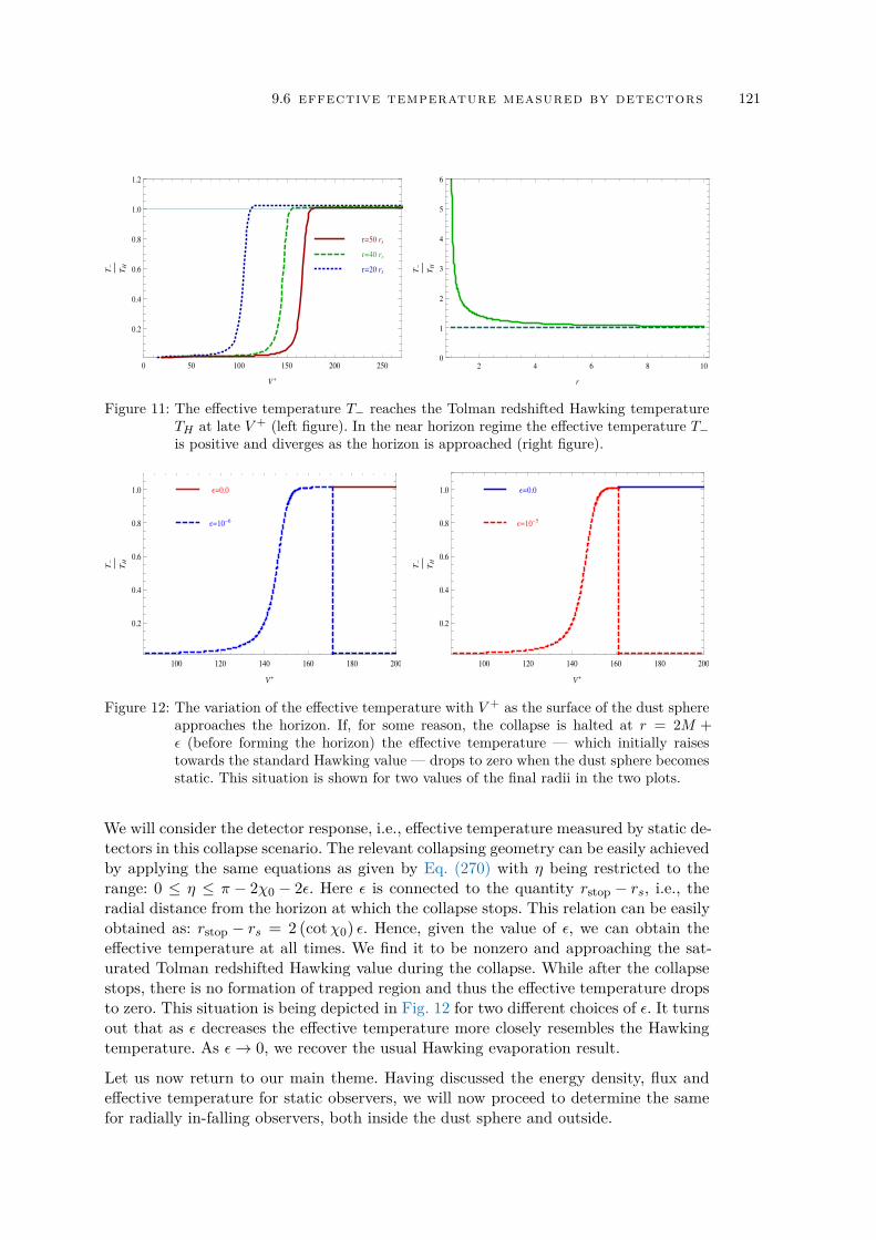
9.6 effective temperature measured by detectors 121

r=50 rs

r=40 rs

r=20 rs

0 50 100 150 200 250

0.2

0.4

0.6

0.8

1.0

1.2

V+

T-

TH

2 4 6 8 10

0

1

2

3

4

5

6

r

T-

TH

Figure 11: The effective temperature T− reaches the Tolman redshifted Hawking temperatureTH at late V + (left figure). In the near horizon regime the effective temperature T−is positive and diverges as the horizon is approached (right figure).

e=0.0

e=10-6

100 120 140 160 180 200

0.2

0.4

0.6

0.8

1.0

V+

T-

TH

Ε=0.0

Ε=10-5

100 120 140 160 180 200

0.2

0.4

0.6

0.8

1.0

V+

T-

TH

Figure 12: The variation of the effective temperature with V + as the surface of the dust sphereapproaches the horizon. If, for some reason, the collapse is halted at r = 2M +ε (before forming the horizon) the effective temperature — which initially raisestowards the standard Hawking value — drops to zero when the dust sphere becomesstatic. This situation is shown for two values of the final radii in the two plots.

We will consider the detector response, i.e., effective temperature measured by static de-tectors in this collapse scenario. The relevant collapsing geometry can be easily achievedby applying the same equations as given by Eq. (270) with η being restricted to therange: 0 ≤ η ≤ π − 2χ0 − 2ε. Here ε is connected to the quantity rstop − rs, i.e., theradial distance from the horizon at which the collapse stops. This relation can be easilyobtained as: rstop − rs = 2 (cotχ0) ε. Hence, given the value of ε, we can obtain theeffective temperature at all times. We find it to be nonzero and approaching the sat-urated Tolman redshifted Hawking value during the collapse. While after the collapsestops, there is no formation of trapped region and thus the effective temperature dropsto zero. This situation is being depicted in Fig. 12 for two different choices of ε. It turnsout that as ε decreases the effective temperature more closely resembles the Hawkingtemperature. As ε→ 0, we recover the usual Hawking evaporation result.

Let us now return to our main theme. Having discussed the energy density, flux andeffective temperature for static observers, we will now proceed to determine the samefor radially in-falling observers, both inside the dust sphere and outside.

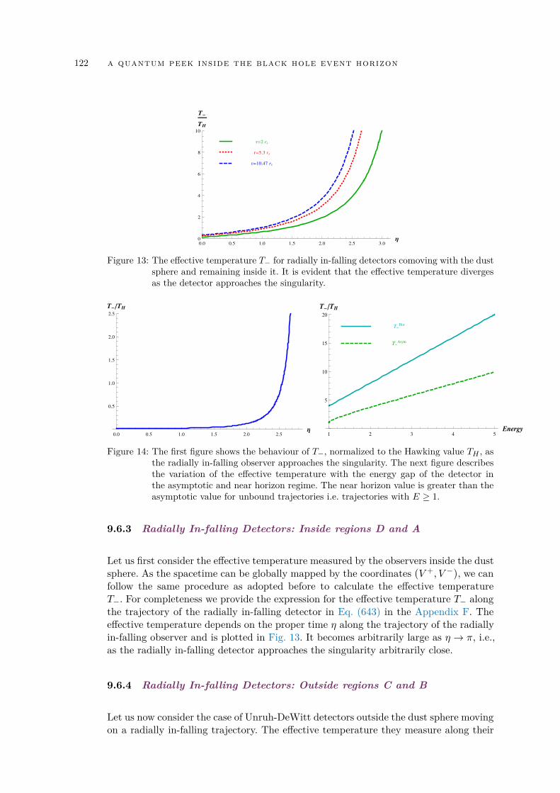
122 a quantum peek inside the black hole event horizon

r=2 rs

r=5.3 rs

r=10.47 rs

0.0 0.5 1.0 1.5 2.0 2.5 3.0Η0

2

4

6

8

10

T-

TH

Figure 13: The effective temperature T− for radially in-falling detectors comoving with the dustsphere and remaining inside it. It is evident that the effective temperature divergesas the detector approaches the singularity.

0.0 0.5 1.0 1.5 2.0 2.5Η

0.5

1.0

1.5

2.0

2.5

T-TH

T-

Hor

T-

Asym

1 2 3 4 5Energy

5

10

15

20

T-

TH

Figure 14: The first figure shows the behaviour of T−, normalized to the Hawking value TH , asthe radially in-falling observer approaches the singularity. The next figure describesthe variation of the effective temperature with the energy gap of the detector inthe asymptotic and near horizon regime. The near horizon value is greater than theasymptotic value for unbound trajectories i.e. trajectories with E ≥ 1.

9.6.3 Radially In-falling Detectors: Inside regions D and A

Let us first consider the effective temperature measured by the observers inside the dustsphere. As the spacetime can be globally mapped by the coordinates (V +,V −), we canfollow the same procedure as adopted before to calculate the effective temperatureT−. For completeness we provide the expression for the effective temperature T− alongthe trajectory of the radially in-falling detector in Eq. (643) in the Appendix F. Theeffective temperature depends on the proper time η along the trajectory of the radiallyin-falling observer and is plotted in Fig. 13. It becomes arbitrarily large as η → π, i.e.,as the radially in-falling detector approaches the singularity arbitrarily close.

9.6.4 Radially In-falling Detectors: Outside regions C and B

Let us now consider the case of Unruh-DeWitt detectors outside the dust sphere movingon a radially in-falling trajectory. The effective temperature they measure along their

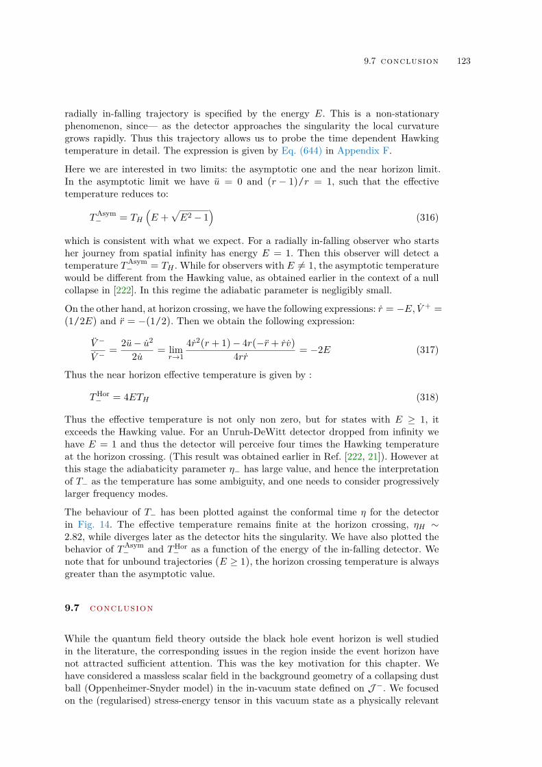
9.7 conclusion 123

radially in-falling trajectory is specified by the energy E. This is a non-stationaryphenomenon, since— as the detector approaches the singularity the local curvaturegrows rapidly. Thus this trajectory allows us to probe the time dependent Hawkingtemperature in detail. The expression is given by Eq. (644) in Appendix F.

Here we are interested in two limits: the asymptotic one and the near horizon limit.In the asymptotic limit we have u = 0 and (r − 1)/r = 1, such that the effectivetemperature reduces to:

TAsym− = TH

(E +

√E2 − 1

)(316)

which is consistent with what we expect. For a radially in-falling observer who startsher journey from spatial infinity has energy E = 1. Then this observer will detect atemperature TAsym

− = TH . While for observers with E 6= 1, the asymptotic temperaturewould be different from the Hawking value, as obtained earlier in the context of a nullcollapse in [222]. In this regime the adiabatic parameter is negligibly small.

On the other hand, at horizon crossing, we have the following expressions: r = −E, V + =(1/2E) and r = −(1/2). Then we obtain the following expression:

V −

V −=

2u− u2

2u = limr→1

4r2(r+ 1)− 4r(−r+ rv)

4rr = −2E (317)

Thus the near horizon effective temperature is given by :

THor− = 4ETH (318)

Thus the effective temperature is not only non zero, but for states with E ≥ 1, itexceeds the Hawking value. For an Unruh-DeWitt detector dropped from infinity wehave E = 1 and thus the detector will perceive four times the Hawking temperatureat the horizon crossing. (This result was obtained earlier in Ref. [222, 21]). However atthis stage the adiabaticity parameter η− has large value, and hence the interpretationof T− as the temperature has some ambiguity, and one needs to consider progressivelylarger frequency modes.

The behaviour of T− has been plotted against the conformal time η for the detectorin Fig. 14. The effective temperature remains finite at the horizon crossing, ηH ∼2.82, while diverges later as the detector hits the singularity. We have also plotted thebehavior of TAsym

− and THor− as a function of the energy of the in-falling detector. We

note that for unbound trajectories (E ≥ 1), the horizon crossing temperature is alwaysgreater than the asymptotic value.

9.7 conclusion

While the quantum field theory outside the black hole event horizon is well studiedin the literature, the corresponding issues in the region inside the event horizon havenot attracted sufficient attention. This was the key motivation for this chapter. Wehave considered a massless scalar field in the background geometry of a collapsing dustball (Oppenheimer-Snyder model) in the in-vacuum state defined on J −. We focusedon the (regularised) stress-energy tensor in this vacuum state as a physically relevant

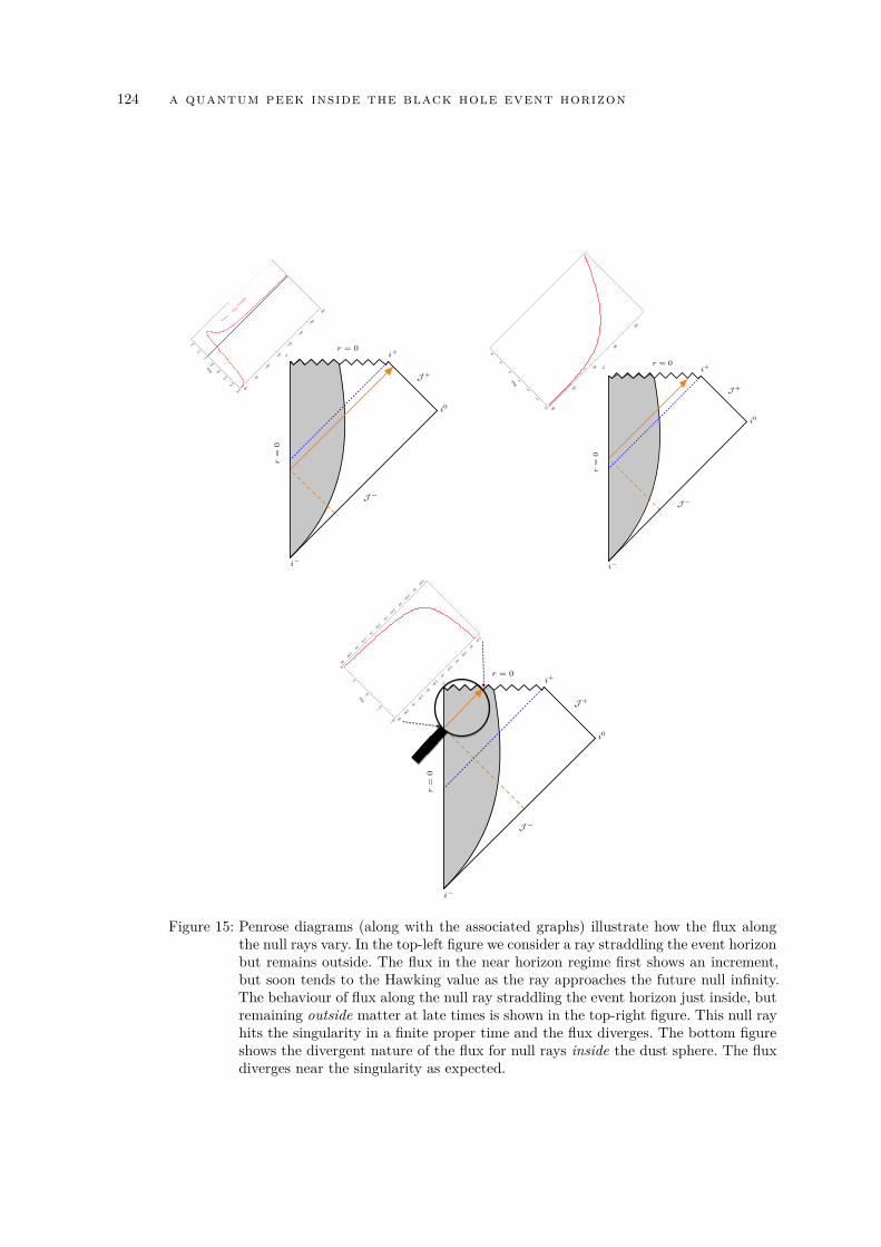
124 a quantum peek inside the black hole event horizon

1

U Hor-U=0

.001

60

80

100

120

140

160

180

200

0.0

0.2

0.4

0.6

0.8

1.0

1.2

1.4

V+

Flux

i

i0

i+r = 0

J

J +

r=

0

1

60

62

64

66

68

0

1

2

3

4

5

6

V+

Flux

i

i0

i+r = 0

J

J +

r=

0

1

60

60.5

61

61.5

62

62.5

63

63.5

64

64.5

65

65.5

-20

-15

-10

-5

060

60.5

61

61.5

62

62.5

63

63.5

64

64.5

65

65.5

V+

Flux

i

i0

i+r = 0

J

J +

r=

0

Figure 15: Penrose diagrams (along with the associated graphs) illustrate how the flux alongthe null rays vary. In the top-left figure we consider a ray straddling the event horizonbut remains outside. The flux in the near horizon regime first shows an increment,but soon tends to the Hawking value as the ray approaches the future null infinity.The behaviour of flux along the null ray straddling the event horizon just inside, butremaining outside matter at late times is shown in the top-right figure. This null rayhits the singularity in a finite proper time and the flux diverges. The bottom figureshows the divergent nature of the flux for null rays inside the dust sphere. The fluxdiverges near the singularity as expected.

9.7 conclusion 125

diagnostic of the quantum effects. The stress-energy tensor, in turn, leads to two scalarobservables – energy density and flux in the normal direction – related to an observerat any point in the spacetime. The key results obtained through this analysis aresummarized below:

• Let us first start with the radially in-falling observers inside the dust sphere andthe invariant observables they measure along their trajectory.

1. In (1+1) spacetime dimensions the radially in-falling observers inside thedust sphere find that the corresponding energy density and flux becomesarbitrarily large as they approach the singularity (arbitrarily close) in afinite proper time. Even though the energy density of the dust ball (ρ) itselfdiverges as the singularity is approached, scalar field energy density (U)diverges faster. The same conclusion holds for the total energy within aninfinitesimal volume as well. Hence in (1+1) spacetime dimensions the scalarfield dominates over the classical source.

2. In (3+ 1) spacetime dimensions also the energy densities of both the scalarfield and classical matter becomes arbitrarily large close to the singularity.Just as in (1+1), in (3+ 1) as well the scalar field energy density dominatesover the classical source. Thus backreaction is important inside the dustsphere.

• The second class of observers we consider are the radially in-falling observersoutside the dust sphere. For them, we arrive at the following conclusions for theinvariant observables:

1. In (1+1) spacetime dimensions, radially in-falling observers outside the dustsphere find that the energy density of the scalar field becomes arbitrarilylarge near the singularity. The same is also true for fluxes measured by theseradially in-falling observers near the singularity. Since there is no classicalmatter present in this region this divergent energy of the scalar field has thepotential to alter the singularity structure.

2. The corresponding situation in the (3 + 1) spacetime dimensions is similarand both the energy density and flux diverge as the singularity is approached.The divergence in the energy density of the scalar field can prohibit theformation of singularity itself due to existence of back-reaction near thesingularity.

Thus, the energy density in the scalar field dominates over the classical back-ground energy density making the backreaction important both inside and out-side the dust sphere. All these conclusions hold for energy density and flux asmeasured along the events in the null rays hitting the singularity either insidethe dust sphere or outside.

• The radially in-falling observers outside the dust sphere observe that there isnothing peculiar at the event horizon; neither the energy density nor the fluxdiverges there.

• The study of the events along the null ray straddling on the outside of the eventhorizon leads to the standard Hawking energy density and flux at late times,while the events along the ray inside the horizon sees an increase of both energy

126 a quantum peek inside the black hole event horizon

density and flux to arbitrarily high values as it approaches near the singularity.Even though derived in (1+1) spacetime dimensions, the same results hold in(3 + 1) spacetime dimensions as well, with milder divergences.

In addition to the above main results, we have also obtained several results for theobservers on the outside of the event horizon which agree with the previous studiesand expectations. Also, for completeness, we have studied the effective temperatureformalism and observed similar effects of divergence at the singularity in this case aswell.

10INFORMATION RETRIEVAL FROM BLACK HOLES

10.1 introduction : black hole information paradox

Evaporation of black holes threatens the most basic and fundamental feature of thestandard quantum theory, namely unitary evolution if one tries extrapolating the resultsobtained at the semi-classical level [106]. Existence of black hole entropy [26, 234] alongwith evaporation of black holes by emission of a (nearly) thermal radiation of positiveenergy due to quantum effects [106] leads to a thermodynamical description of blackholes. Further the flux of negative energy flowing into the black hole decreases its massand the mass lost by the black hole appears in the form of energy of the thermalradiation. Even though this is essential for the celebrated thermodynamic descriptionof black holes, such a process, together with other properties of black holes, appears toviolate the standard unitary quantum mechanics leading to information loss paradox[158]. The crux of the paradox can be summarized as follows — as the black holeevaporates completely without leaving any remnant behind, one can assume that theentire information content of the collapsing body is either destroyed or must be encodedin the resulting radiation. However, residual radiation in this process being (dominantly)thermal, is unable to contain much of the information and hence incapable of makingthe theory unitary. Therefore, most of the information content of the matter whichforms the black hole becomes unavailable to the future asymptotic observers.

In this chapter, we will argue that the version of the paradox concerning the informationcontent of the initial data originates from a hybrid analysis of a process which shouldbe fully quantum mechanical in nature. The matter which forms a black hole in thefirst place, should also be treated as fundamentally quantum mechanical and hencemust follow a quantum evolution. We expect that the classical description at lowestorder leads to formation of an event horizon but the information about the quantumnature of the collapsing material must not be completely ignored while studying thisprocess. The quantum matter forming the black hole will populate its modes at futureasymptotia non-thermally and the presence of this effect can be felt even in semi-classical level.

Previously it has been shown that the particle content of the ingoing field modes makesthe resulting Hawking radiation to be supplemented by a stimulated emission. There-fore, the radiation profile becomes non-thermal and thus capable of storing information.There have been studies (see e.g., [242, 199, 223, 19, 197, 217, 169, 2]) regarding in-formation content of corrected spectrum, form the point of view of information theory(Von Neumann entropy, channel capacity, etc.). We, however, do not commit to a par-ticular specification of the information content but concentrate on the possibility ofexplicit reconstruction of the initial state of the field from the resultant radiation in acollapse process. Neither do we make an attempt to restore unitarity by such a stimu-

127

128 information retrieval from black holes

lated emission process. Our focus will be to reconstruct the initial data to the extentpossible when the Hawking radiation has a non-thermal part.

We will see that the symmetry characteristics of the initial state will determine whetherasymptotic observers can reconstruct the initial state completely or partially. Therefore,analysis of the allowed set of symmetries present in the characterization of the initialstate will play a pivotal role in the recovery of the initial information content, just fromthe spectrum function when the black hole is evaporated completely. Recently, it hasbeen shown [63] how to reconstruct a qubit state which is thrown into a black holeby measuring changes in the black hole characteristics in such a process. Our schemeis somewhat similar in spirit, but calculates the projection of states in an infinitedimensional Hilbert space.

In the semi-classical approximation, the formation of the classical event horizon isunavoidable, since the part forming the black hole follows classical equations of motion.With the presence of the horizon, pure to mixed state transition is also imminent. Thusa part of the field modes always remain hidden from the asymptotic observer, givingrise to a mixed state description. We show that, at the semi-classical level itself, thereare additional quantum hairs in the resulting radiation profile. At this stage we shouldemphasize that we are not focusing on the non-thermal distortions originating fromthe vacuum itself, but on the part which is originating from non-vacuum component ofthe quantum state. As discussed earlier [241, 101], there can be various sources of non-thermal corrections, even when the initial state is a vacuum. We dub the total Hawkingradiation endowed with all these corrections, as the vacuum response. We show that ifthere are corrections over and above the vacuum response, information regarding theinitial sector of Hilbert space, which formed the black hole, can be extracted.

Information in an initial state of a collapsing field carrying non-zero stress energy canbe stored using a superposed state in the Hilbert space. We will be using initial non-vacuum state of the form:

|Ψ〉in =∫ ∞

0

dω√4πω

f(ω)a†(ω)|0〉in. (319)

This is an excited state which is a superposition of one-particle states. The functionf(ω) completely encodes the information about the initial state and the idea is toreconstruct this function from the spectrum of the black hole radiation received byasymptotic observers.

We will first show how this reconstruction of initial state works, for a collapse modelforming Schwarzschild black hole in (3 + 1) dimension as a quasi-static process. Thus,we first consider the case in which a spherically symmetric scalar field is undergoing acollapse process to form a black hole. The complete quantum analysis of this processwill require the study of the quantum evolution of the field as well as that of the“quantum geometry” and the back-reaction. However, lack of good control over eitherthe quantum sector of the geometry or the back-reaction in (3+ 1) dimension, compelsus to adopt a semi-classical approach, where we take the matter field to be describedby:

φ(x) = φ0I + δφ, (320)

10.2 initial state of spherical collapse 129

where φ0 is the part which dominantly describes the evolution of geometry. Thatis,

〈Ψ|Tµν [φ]|Ψ〉 ∼ 〈Ψ|Tµν [φ0]|Ψ〉,

will act as the source for the geometry and will lead to the gravitational collapse. Wecan, alternatively, think of a process in which some of the highly excited modes φ0 of thefield, acting as classical matter, collapse to form a black hole, while some other modes δφevolve quantum mechanically as a test field in this background. These quantum modesare populated, i.e., such modes will be in a non-vacuum state of the field and carrysome small amount of energy into the black hole. Classically, the test field modes, oncethey cross the horizon, will make the black hole larger and then will become inaccessibleto future asymptotic observers. However, quantum mechanically, we show that such aprocess will lead to a non-vacuum distortion in the late time Hawking radiation whichwill make the recovery of information about the initial quantum state possible. Thelate time radiation will have a frequency space correlation which becomes non-zero ifthe initial state was not a vacuum.

We will also discuss a (1+ 1) dimensional dilatonic black hole solution which is knownas the CGHS model. This model includes the effect of the back-reaction, in which theproblem of forming a black hole with quantum matter as source can be solved exactly.Therefore, in this model, we will be able to not only account for the back-reaction of thetest field modes δφ but also recover the information about the field φ0 which forms theblack hole itself. Further, being a conformally flat spacetime, the Bogoliubov coefficientscan be calculated exactly and hence the information content in the out-going modescan be obtained at any stage of evolution, not only at late times. Thus, we can trackthe loss of information, if any, during the course of evolution and evaporation.

In Section 10.2 and Section 10.3, we discuss the characterization of the initial statewe will be dealing with in this chapter. We will also briefly discuss quantum fieldmodes in a spherically symmetric black hole collapse scenario. These modes will beused to specify the non-vacuum state of the test field in the spherically symmetric case.In Section 10.4, we discuss the resulting correlation spectrum from such non-vacuum,single particle states. Since accommodating the back-reaction in the (3+ 1) black holeformation is technically very difficult, we go to lower dimensions to get a handle on theback-reaction analytically. For this purpose we consider the evaporation of a (1 + 1)dimensional dilatonic black hole solution. We will briefly describe this model in Section10.5, and shall connect up with the (3 + 1) results. In Section 10.6, we will show howthe concept of the non-vacuum distortion can be utilized to harness information aboutthe matter falling into the black hole, which normally would have been invisible to theasymptotic (left-moving) observer. We discuss the class of symmetry characteristics ofthe initial state, for which such an asymptotic observer can reconstruct the initial data.In Section 10.7, we will discuss the implication of our scheme of retrieval of informationand the scope for further generalization. The detailed calculations have been presentedin Appendix G.

10.2 initial state of spherical collapse

The case we discuss first is that of a real scalar quantum field living in a collapsingspacetime, which eventually would harbor a black hole. The initial state of the field is

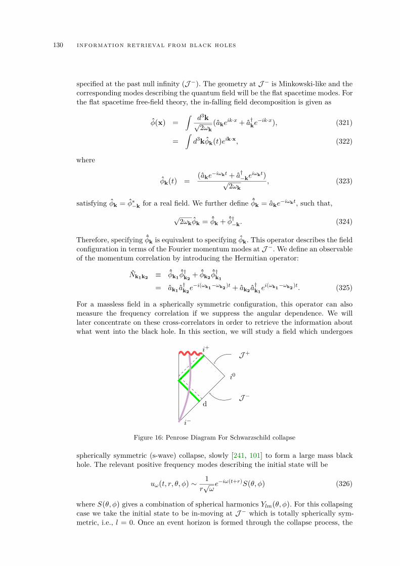
130 information retrieval from black holes

specified at the past null infinity (J −). The geometry at J − is Minkowski-like and thecorresponding modes describing the quantum field will be the flat spacetime modes. Forthe flat spacetime free-field theory, the in-falling field decomposition is given as

φ(x) =∫

d3k√2ωk

(akeik·x + a†ke

−ik·x), (321)

=∫d3kφk(t)e

ik·x, (322)

where

φk(t) =(ake

−iωkt + a†−keiωkt)

√2ωk

, (323)

satisfying φk = φ∗−k for a real field. We further define ˆφk = ake−iωkt, such that,

√2ωkφk = ˆφk + ˆφ†−k. (324)

Therefore, specifying ˆφk is equivalent to specifying φk. This operator describes the fieldconfiguration in terms of the Fourier momentum modes at J −. We define an observableof the momentum correlation by introducing the Hermitian operator:

Nk1k2 ≡ ˆφk1ˆφ†k2

+ ˆφk2ˆφ†k1

= ak1 a†k2e−i(ωk1−ωk2 )t + ak2 a

†k1ei(ωk1−ωk2 )t. (325)

For a massless field in a spherically symmetric configuration, this operator can alsomeasure the frequency correlation if we suppress the angular dependence. We willlater concentrate on these cross-correlators in order to retrieve the information aboutwhat went into the black hole. In this section, we will study a field which undergoes

i+

i−

i0

d

J +

J −

Figure 16: Penrose Diagram For Schwarzschild collapse

spherically symmetric (s-wave) collapse, slowly [241, 101] to form a large mass blackhole. The relevant positive frequency modes describing the initial state will be

uω(t, r, θ,φ) ∼1

r√ωe−iω(t+r)S(θ,φ) (326)

where S(θ,φ) gives a combination of spherical harmonics Ylm(θ,φ). For this collapsingcase we take the initial state to be in-moving at J − which is totally spherically sym-metric, i.e., l = 0. Once an event horizon is formed through the collapse process, the

10.2 initial state of spherical collapse 131

full state can again be described using a combined description at the event horizon Hand on the future null infinity (J +) [185, 204], i.e., the field configuration of spacetimecan also be described using positive and negative frequency modes compatible to J +

as well as on the horizon H. For an asymptotic observer, the end configuration of thefield will be the out-state, described using modes at J +, which are again flat spacetimemodes owing to the asymptotic flatness of the model. The field content of the out-statecan be obtained using the Bogoliubov coefficients between the modes at J − and J +

[185, 204]. The asymptotic form of these Bogoliubov coefficients are given as [106]

αΩω =1

2πκ

√Ωω

exp[πΩ2κ

]exp [i(Ω− ω)d] exp

[iΩκ

log ωC

]Γ[− iΩκ

],

βΩω = − 12πκ

√Ωω

exp[−πΩ

2κ

]exp [i(Ω + ω)d] exp

[iΩκ

log ωC

]Γ[− iΩκ

]. (327)

where Ω is the frequency of the out-modes at J +, the parameter κ is the surfacegravity of the black hole, while C is a product of affine parametrization of incomingand outgoing null rays [185, 204] and d is an arbitrary constant marking the last nullray reaching J +.

We can set d = 0 through co-ordinate transformations on J −. These Bogoliubov coeffi-cients are accurate for large values of ω. At small ω values, the expressions in Eq. (327)will receive corrections. However, when we are interested in the late-time radiation atfuture null infinity (J +), one can show that the dominating spectra will come fromthose modes which have just narrowly escaped the black hole, i.e., which were scat-tered just before the formation of the event horizon. Such modes are the ones withhigh frequencies at the past null infinity. So the calculations done with Eq. (327) willbe accurate to the leading order. We will consider states which are eigenstates of thenumber operator defined with the help of the in-modes, but are not the energy ormomentum eigenstates. Let the state of the field undergoing collapse in a black holespacetime, be a (superposition of) single particle excitation state

|Ψ〉in =∫ ∞

0

dω√4πω

f(ω)a†(ω)|0〉. (328)

(We will generalize the analysis for higher excited states in the appendices, see AppendixG) We define a new function g(z), using a dimensionless variable z, which is related tothe frequency ω of mode functions at J −, as

log ωC

= z ⇒ f(Cez) = g(z), (329)

to re-write the state as

|Ψ〉in =∫ ∞−∞

dz√4πg(z)a†(z)|0〉. (330)

In order to specify the state we need to specify f(ω) in Eq. (328) or equivalently g(z)in Eq. (330). We will see how much of information about this function can be retrieved

132 information retrieval from black holes

from the outgoing modes. Before proceeding to the black hole emission spectra, weintroduce the function

F (y) =∫ ∞−∞

dzg(z)eiyz, (331)

which will be used to characterize the initial state in Eq. (328) or Eq. (330). This isan equally good measure for encoding the information about the state, as it is just aFourier transform of an L2 function. It is useful to construct yet another function

F

(Ωκ

)= exp

[πΩ2κ

]F

(Ωκ

), (332)

from Eq. (331). Then one can obtain the distribution g(t) from Eq. (332) as

g(z) =1

2π

∫ ∞−∞

d

(Ωκ

)F

(Ωκ

)e−i

Ωκze−

πΩ2κ . (333)

We note again that the one particle state is completely specified once we have completeknowledge of the function F (Ω/κ). We will discuss the information about F (Ω/κ)available in the out-going modes, by analyzing the frequency space correlations. Suchcorrelations turn out to be definitive tools for the recovery of the information. We willfirst discuss these correlations briefly in the next section and then go on to study aspecial case of this correlation, the self-correlation, which gives the emission profileof the black hole, and we will show that the emission profile develops a non-vacuum,non-thermal, part capable of storing information.

10.3 information of black hole formation : correlation func-tion

We wish to obtain the information regarding the quantum states falling into the blackhole, or more elaborately, regarding the quantum states which formed the black holeitself. For this purpose, we consider an observable which measures the frequency spacecorrelation in the out-going modes. The annihilation operator bΩ associated with theoutgoing modes is related to the creation and annihilation operator aω and a†ω of theingoing mode as,

bΩ =∫dω(α∗Ωωaω − β∗Ωωa†ω

)(334)

where, αΩω and βΩω are the Bogoliubov coefficients. Now following Eq. (325), thefrequency space correlation for the outgoing modes turns out to yield

NΩ1Ω2 = b†Ω1bΩ2e

−i(Ω1−Ω2)t + b†Ω2bΩ1e

i(Ω1−Ω2)t (335)

Recently, an analogous operator was used in [5] for studying the growth of loop correc-tions in an interacting theory. For the initial state (in-state) of the field, being vacuum|0〉 or one with a definite momentum |k〉 (and hence for all the Fock basis states), theexpectation value of this correlation operator vanishes. We now consider this quantumcorrelation of the field in the out-going modes. The correlation operator NΩ1Ω2 definedin Eq. (335) for the out-going modes is related to those for in-moving modes through

10.3 information of black hole formation : correlation function 133

Bogoliubov transformations, as presented in Eq. (334). If the test field δφ starts inthe in-vacuum state |0〉in, then the expectation value of the frequency correlation be-comes,

in〈0|NΩ1Ω2 |0〉in = δ(Ω1 −Ω2)× e−π(Ω1+Ω2)

2κ

√Ω1Ω2

4π2κ2

×

Γ[−iΩ1

κ

]Γ[iΩ2κ

]e−i(Ω1−Ω2)t + c.c.

(336)

which vanishes identically for the off-diagonal elements and hence the asymptotic fu-ture observer will also measure no frequency correlation in the out-going modes. Thediagonal elements of this observable gives the number spectrum. Such an observer mea-sures the out-going spectrum to be a thermal one which can be verified by takingΩ1 = Ω2.

However, when the test field starts in a non-vacuum state, the out-going modes willdevelop a frequency correlation and the expectation of Eq. (335) will become non-zero.The correction to the expectation of the frequency correlator NΩ1Ω2 in a non-vacuumin-state leads to,

in〈ψ|NΩ1Ω2 |ψ〉in =

(∫ dω√4πω

f(ω)α∗Ω2ω

)

×(∫

dω√4πω

f∗(ω)αΩ1ω

)+

(∫dω√4πω

f∗(ω)β∗Ω2ω

)

×(∫

dω√4πω

f(ω)βΩ1ω

)e−i(Ω1−Ω2)t + c.c (337)

Using the expressions for αΩω and βΩω from Eq. (327), we obtain,

in〈ψ|NΩ1Ω2 |ψ〉in =1

4π [A(Ω1)A(Ω2)∗ + c.c.]

+1

4π [B(Ω1)B(Ω2)∗ + c.c.] . (338)

with

A(Ω) = e−πΩ2κ

√Ω

2πκΓ[−iΩ

κ

]F

(Ωκ

)e−iΩt, (339)

and

B(Ω) = eπΩ2κ

√Ω

2πκΓ[−iΩ

κ

]F ∗(−Ωκ

)e−iΩt (340)

expressed in terms of the time co-ordinate of out-going observers. The frequency cor-relation for two distinctly separated frequencies (i.e., Ω1 6= Ω2), as discussed above,remains zero for all the field configurations which were in the vacuum (incidentally, alsofor configurations in individual Fock basis elements) in the in-state. However, as for theout-state, the frequency correlation remains zero only if the in-state was a vacuum. Theout-going modes develop frequency correlation, even if the in-state was a non-vacuumFock basis state with zero correlation. Alternatively, those fields which carried some

134 information retrieval from black holes

amount of stress energy into the black hole definitely develop some non-zero correlationat late times, while only those fields which were in a vacuum state develop no late timefrequency correlation. Therefore, by just measuring this operator, a late time observerwill be able to tell if some non-zero stress-energy has entered the black hole.

Further the observer can decipher the state that entered into the black hole, by recon-structing F (Ω/κ) from this non-zero expectation value of the correlation. We demon-strate the technique below. We can also consider a special case of this correlation, i.e.,the self-correlation for simplicity. We measure the change in self-correlation, which isjust the spectrum operator [147], once a non-vacuum state perturbs the black holeconfiguration and we will see that this change encodes information of interest (see Ap-pendix G). Expectedly, other correlations carry information about the in-going statesmuch more efficiently.

10.4 radiation from black hole: information about the initialstate

We show that Eq. (338) can be used by out-moving observers for retrieving informationregarding F (Ω) and thus for reconstructing the state presented in Eq. (319). From theoff-diagonal elements of Eq. (338) we construct a complex quantity

DΩ1Ω2 ≡ NΩ1Ω2 +i

∆Ω∂

∂tNΩ1Ω2 , (341)

where ∆Ω = Ω1 −Ω2. In terms of the function F (Ω/κ), the above expression can bere-written as

DΩ1Ω2 =1

2π

√Ω1Ω2

4π2κ2 Γ[−iΩ1

κ

]Γ[iΩ2κ

]eπ(Ω1+Ω2)2κ F

(−Ω2κ

)F ∗(−Ω1κ

)

+ e−π(Ω1+Ω2)

2κ F

(Ω1κ

)F ∗(

Ω2κ

)e−i(Ω1−Ω2)t.

(342)

For a real initial state, we have F (Ω/κ) = F ∗(−Ω/κ) and therefore, Eq. (342) can beused to extract the function F (Ω/κ) as,

SΩ1Ω2 ≡4π3κ2√

Ω1Ω2

DΩ1Ω2ei(Ω1−Ω2)t

Γ[−iΩ1

κ

]Γ[iΩ2κ

]cosh

(π(Ω1+Ω2)

2κ

)= F

(Ω1κ

)F ∗(

Ω2κ

). (343)

Clearly, left hand side of Eq. (343) can be determined by observing the emission spec-trum. Therefore, left hand side is under our control completely. From the above relation,we see that this quantity has to be separable as a product in terms of the frequencies Ω1

10.4 radiation from black hole: information about the initial state 135

and Ω2. Using this property, we can obtain the function F (Ω/κ), upto an irrelevantconstant phase, from the symmetric sum

logSΩ1Ω2 = logF(

Ω1κ

)+ logF ∗

(Ω2κ

), (344)

or, alternatively, by fixing one of the frequencies and varying the other. Therefore, forthe real initial state, the state can be identically and completely reconstructed fromcorrelations in the out-going modes.

In [146], we devised a formalism to deal with the analysis of field content of a non-vacuum pure state corresponding to a particular observer with respect to another set ofobservers, using the correlation functions. The information about the state through thefunction f(ω), together with the Bogoliubov coefficients, completely characterize thedeviations form the standard vacuum response. The analysis of the spectrum operator[197, 32] also captures this distortion. The extraction of information about initial datausing the spectral distortion NΩ = 〈Ψ|b†ΩbΩ|Ψ〉 − 〈0|b†ΩbΩ|0〉, as reported in [147] ispresented in detail in Appendix G.1. In Appendix G.2, we show that for a particularclass of symmetric initial states, interesting quantities can be obtained from the out-states. Higher order correlation functions will give the information regarding the manyparticle sectors subsequently. However, in this chapter, we only focus on the singleparticle case, for simplicity.

We have thus demonstrated the existence of semi-classical hairs in the case of thespherically symmetric collapse which would have formed a Schwarzschild black holeclassically. We learn that if we are aware of the symmetries of the system which isgoing to form a black hole, from some general principles, we will know how the non-vacuum response would look like. We can measure particle content for different testfields. The test field which contributes infinitesimal energy to the formation will reflectits non-vacuum character in the late time radiation. That is to say, its spectra will showdeviations from the expected vacuum response, corresponding to the symmetries ofinitial data. Measurements of such non-vacuum distortion will reveal partial or completecharacter of the state of the field depending on the knowledge of the symmetry of initialprofile.

The cases discussed above were all based on test field approximations. We can extrap-olate this idea to conjecture that if we have correct account of the back-reaction, orquantum gravity corrected Bogoliubov coefficients, they will still provide a handle forinitial data as in Eq. (342) (see also Eq. (645) in Appendix G). It will be worthwhile todemonstrate these ideas for a set-up including the back-reaction. In a general (3 + 1)collapse scenario the precise handling of back-reaction remains an open problem. Evenfor the spherical collapse case, which we discussed above, accounting for the back-reaction is a tedious task. We will instead be looking at a (1+ 1) dimensional dilatonicCGHS black hole model. In this case the issue of back-reaction can be exactly han-dled and even the full quantum gravity calculation can be implemented perturbatively.However, in this chapter, we will be content with the semi-classical scheme whereinthe back-reaction of the test field has been accounted for. We will see how the non-vacuum distortions lead to additional quantum hairs, which would have been missedclassically.

136 information retrieval from black holes

10.5 cghs model: introduction

The CGHS black hole solution [44, 86] is a (1 + 1) dimensional gravity model of adilatonic field φ (along with possibly other matter fields). The theory is described bythe action,

A =1

2π

∫d2x√−g

[e−2φ

(R+ 4(∇φ)2 + 4λ2

)− 1

2

N∑i=1

(∇fi)2]

(345)

where λ2 is the cosmological constant and fi stands for i− th matter field; N suchtotal fields may be present. Since all two dimensional space-times are conformally flatthe metric ansatz will involve a single unknown function, the conformal factor, whichis written in double null coordinates as,

ds2 = −e2ρdx+dx−. (346)

For the matter fields, the classical solutions are those in which, fi(x+,x−) = fi+(x+) +fi−(x−). Then, given some particular matter fields, one can obtain corresponding so-lutions for φ and ρ respectively. The simplest among all of them corresponds to thevacuum solution in which e−2ρ = e−2φ = (M/λ)− λ2x+x−. This represents a blackhole of mass M , with line element,

ds2 = − dx+dx−

Mλ − λ2x+x−

, (347)

while in absence of any mass, i.e.,M = 0 we obtain the linear dilatonic vacuum solutionsas

ds2 = − dx+dx−

−λ2x+x−. (348)

A more realistic and dynamical situation corresponds to the case when an in-comingmatter forms a singularity. If the matter starts at x+i and extends up to x+f , then theline element turns out to be,

ds2 = − dx+dx−

M(x+)λ − λ2x+x− − P+(x+)x+

, (349)

where M(x+) and P+(x+) correspond to the integrals,

M(x+) =∫ x+

x+i

dy+y+T++(y+), (350)

P+(x+) =∫ x+

x+i

dy+T++(y+). (351)

The region outside x+f is a black hole of mass M ≡ M(x+f ). One can check that thereis a curvature singularity where the conformal factor diverges.

The singularity hides behind an event horizon for future null observers receiving the out-moving radiation. The location of the event horizon can be obtained starting from the

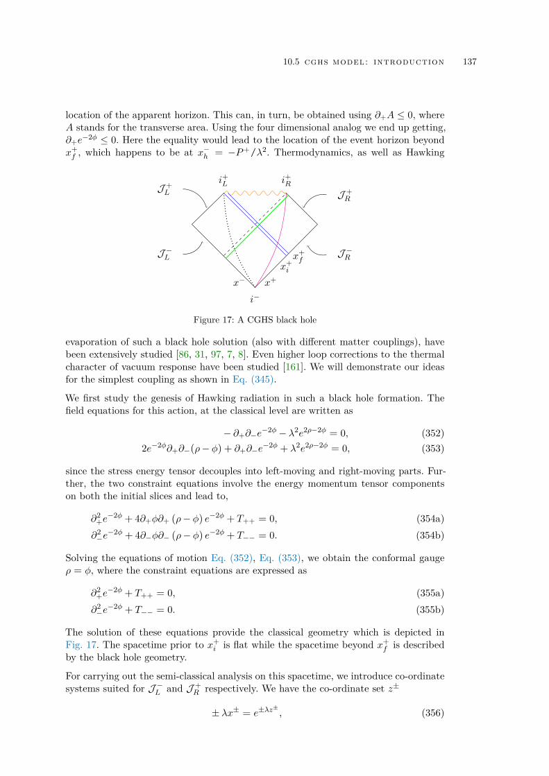
10.5 cghs model: introduction 137

location of the apparent horizon. This can, in turn, be obtained using ∂+A ≤ 0, whereA stands for the transverse area. Using the four dimensional analog we end up getting,∂+e

−2φ ≤ 0. Here the equality would lead to the location of the event horizon beyondx+f , which happens to be at x−h = −P+/λ2. Thermodynamics, as well as Hawking

J +R

J −Rx+i

x−

J +L

J −L x+f

x+

i+L i+R

i−

Figure 17: A CGHS black hole

evaporation of such a black hole solution (also with different matter couplings), havebeen extensively studied [86, 31, 97, 7, 8]. Even higher loop corrections to the thermalcharacter of vacuum response have been studied [161]. We will demonstrate our ideasfor the simplest coupling as shown in Eq. (345).

We first study the genesis of Hawking radiation in such a black hole formation. Thefield equations for this action, at the classical level are written as

− ∂+∂−e−2φ − λ2e2ρ−2φ = 0, (352)2e−2φ∂+∂−(ρ− φ) + ∂+∂−e

−2φ + λ2e2ρ−2φ = 0, (353)

since the stress energy tensor decouples into left-moving and right-moving parts. Fur-ther, the two constraint equations involve the energy momentum tensor componentson both the initial slices and lead to,

∂2+e−2φ + 4∂+φ∂+ (ρ− φ) e−2φ + T++ = 0, (354a)

∂2−e−2φ + 4∂−φ∂− (ρ− φ) e−2φ + T−− = 0. (354b)

Solving the equations of motion Eq. (352), Eq. (353), we obtain the conformal gaugeρ = φ, where the constraint equations are expressed as

∂2+e−2φ + T++ = 0, (355a)

∂2−e−2φ + T−− = 0. (355b)

The solution of these equations provide the classical geometry which is depicted inFig. 17. The spacetime prior to x+i is flat while the spacetime beyond x+f is describedby the black hole geometry.

For carrying out the semi-classical analysis on this spacetime, we introduce co-ordinatesystems suited for J −L and J +

R respectively. We have the co-ordinate set z±

± λx± = e±λz± , (356)

138 information retrieval from black holes

which maps the entire J −L into z− ∈ (−∞,∞). We obtain another co-ordinate systemsuited for J +

R as σ±out. Let us first discuss the transformation between (z+, z−) and(σ+out,σ−out) defined as

z+ = σ+out; z− = − 1λ

ln[e−λσ

−out +

P+

λ

]. (357)

The horizon, located at x− = −P+/λ2, will get mapped to z− = z−i = − 1λ log (P+/λ)

in these co-ordinates. ‘In’ state modes are defined on the asymptotically flat region J −Lmoving towards J +

R and the convenient basis modes can be taken to be,

uω =1√2ωe−iωz

− , (358)

where ω > 0. The ‘out’ region corresponds to J +R which receives the state from J −L

after the black hole has formed. The basis modes in the out region at J +R are

vω =1√2ωe−iωσ

−out Θ(z−i − z

−), (359)

where Θ is the usual step function arising from the fact that the out modes are sup-ported by states on J −L only in the interval (−∞, 0). Again the field can be specifiedfully on J −L or jointly on J +

R and on the event horizon HR. Since the mode functionsat HR correspond to part of the field falling into the singularity, which cannot be de-tected by observers at J +

R , they need to be traced over. Thus, the precise form of modedecomposition on HR does not affect physical results for J −L . Therefore, we can expandthe dilaton field in a different mode basis as,

f =∫ ∞

0dω

[aωuω + a†ωu

∗ω

], (in) (360)

=∫ ∞

0dω

[bωvω + b†ωv

∗ω + bωvω + b†ωv

∗ω

], (out) (361)

where a†ω corresponds to creation operator appropriate for the ‘in’ region. Similarly b†ωand b†ω stand for the creation operators for the ‘out’ region and the black hole interiorregion respectively. The inner product between vΩ and u∗ω corresponds to,

αΩω = − iπ

∫ z−i

−∞dz−vΩ∂−u

∗ω

=1

2π

√ω

Ω

∫ z−i

−∞dz− exp

[iΩλ

ln(

e−λz− − P+

λ

)+ iωz−

]

=1

2πλ

√ω

Ω

(P+

λ

)i(Ω−ω)/λB

(− iΩλ

+iω

λ, 1 + iΩ

λ

), (362)

10.6 information regarding the collapsing matter 139

while the inner product between vΩ and uω gives

βΩω =i

π

∫ z−i

−∞dz−vΩ∂−uω

=1

2π

√ω

Ω

∫ z−i

−∞dz− exp

[iΩλ

ln(

e−λz− − P+

λ

)− iωz−

]

=1

2πλ

√ω

Ω

(P+

λ

)i(Ω+ω)/λ

B

(− iΩλ− iω

λ, 1 + iΩ

λ

), (363)

whereB(x, y) is the Beta function. The vacuum response can be obtained from Eq. (363),which has a thermal profile in the limit of large frequencies, which will be the late timelimit for observers at J +

R . In general the vacuum response also comes with a non-thermal part. This late-time thermal response originates from the vacuum state at J −L .But, due to asymmetry in the left- and right-moving modes, the modes which formthe black hole, originate only from J −R , rather than from J −L . If one has to retrievethe information regarding the quantum states that formed the black hole in the firstplace, the observers moving left are the relevant ones. Therefore, we will concentrateon the future, left moving, observers who are moving in the flat spacetime throughout.We want to study the black hole evaporation at the semi-classical level for one suchobserver, which we will do in the next section.

10.6 information regarding the collapsing matter

The left-moving matter is introduced for x+ ≥ x+i and hence the spacetime is in avacuum configuration prior to it. The spacetime, in the region x+ < x+i is flat and themetric is given as in the Eq. (348), which, on using the co-ordinates

x+ = − 1λy+

; x− = − 1λy−

, (364)

remains the same

ds2 = − dy+dy−

−λ2y+y−. (365)

The location x+i is marked by y+i = −1/λx+i . Using another set of co-ordinate trans-formation the metric on J −R can be brought into the flat form. A left-moving observerwho completely stays in the region in the past of J +

L remains in flat spacetime.

140 information retrieval from black holes

However, such an observer is able to access only portion of initial data on J −R . Therefore,the Bogoliubov coefficients between a complete set of mode functions uω defined on J −Rand the complete set of mode functions vω defined on J +

L , are given as

αΩω = − iπ

∫ χ+i

−∞dχ+vΩ∂−u

∗ω

=1

2π

√ω

Ω

∫ χ+i

−∞dχ+ exp

[iΩλ

ln(e−λχ

+ − |y+i |)

+ iωχ+]

=1

2πλ

√ω

Ω|y+i |

i(Ω−ω)λ B

(− iΩλ

+iω

λ, 1 + iΩ

λ

), (366)

and

βΩω =i

π

∫ χ+i

−∞dχ+vΩ∂+uω

=1

2π

√ω

Ω

∫ χ+i

−∞dχ+ exp

[iΩλ

ln(e−λχ

+ − |y+i |)− iωχ+

]=

12πλ

√ω

Ω|y+i |

i(Ω+ω)λ B

(− iΩλ− iω

λ, 1 + iΩ

λ

). (367)

Thus, as before, the observer at J +L will observe Bogoliubov coefficients similar to the

ones observed by their right counterparts but with the parameter exchange |y+i | ↔P+/λ [143]. However, these nontrivial Bogoliubov coefficients are totally due to thetracing over of the modes which lie in the future of J +

L and not due to any geometrychange. One can check that if the fraction of the tracing over vanishes, which corre-sponds to the limit |y+i | → 0, the Bogoliubov coefficients will assume a trivial form.Along identical lines, the Bogoliubov coefficients in Eq. (362) and Eq. (363) assumea trivial form in the limit P+ → 0. For these observers the effect of tracing over isindistinguishable from that of geometry change. Both these effects vanish simultane-ously in the above limit. However, the vacuum response for both these observers isindistinguishable. Late time radiation for such observers on J +

L for the vacuum state(of a test field) on J −R is also thermal with the same temperature as measured by theirright-moving counterparts !

Further, any non vacuum state on J −R will lead to non-vacuum distortions in the radia-tion. We will now use the Bogoliubov coefficients for extracting information regardingthe matter that formed the black hole.

10.6.1 Test Field approximation

To start with, we can first do a quick demonstration, under the test field approximation,in order to connect up with the earlier case of the Schwarzschild black hole, by assumingthat the matter φ forming the black hole is classical. Then we add a little more matterδφ to the black hole perturbatively. That is to say, we add another small matter pulseto the collapse with support in the region x+ > x+f . This small chunk is to be treatedperturbatively as quantum matter. Given the form of the Bogoliubov coefficients as inEq. (366) and Eq. (367), we note that they remain independent of the matter contentin the region x+ > x+i and solely depend on the co-ordinate at which the first matter

10.6 information regarding the collapsing matter 141

shell was introduced, which serves as a horizon for the left-moving observers. Therefore,an asymptotically left-moving observer will use Eq. (366) and Eq. (367) to computethe spectral distortion and reconstruct the state of the test matter which is thrown in,through a procedure similar to what was done for the Schwarzschild black hole. Then,for asymptotic observers at late times, the high frequency approximation of Eq. (366)and Eq. (367) leads to a form exactly as in Eq. (327). Thus, for such observers, theresults developed in Section 10.4 and Appendix G.2 are exactly applicable.

10.6.2 Adding back-reaction: Extracting information about the matter form-ing the black hole

In the CGHS case, we can do away with the high frequency approximation to exactlycalculate the results for observers at any finite time (not necessarily at late times) aswell. Moreover, the results derived for the left-moving asymptotic observers remainsoblivious to the matter introduced beyond their perceived horizon and hence does notcare about the geometry beyond the horizon as well. Therefore, all the back-reaction ofthe collapsing matter can now be accounted for, since they do not change the geometryprofile of left-moving observers at all. Being a conformally flat spacetime, we know theexact mode functions irrespective of the back-reaction in the entire spacetime as wellas in the relevant left portion. Therefore, the form of Eq. (366) and Eq. (367) are exact,even in the presence of back-reaction of the field, or even when we take the collapsingmatter φ itself to be quantum matter, which we will do next.

For a complete semi-classical treatment, we take the field φ to be quantum mechanical.At the semi-classical level, the stress energy tensor components are replaced by theirexpectation values 〈T±±〉 and 〈T+−〉. Being a two dimensional spacetime the expecta-tion values get an additional contribution from the conformal anomaly. Therefore, theclassical equations (for N = 1) are modified to

− ∂+∂−e−2φ − λ2e2ρ−2φ =1

12π∂+∂−ρ, (368)

2e−2φ∂+∂−(ρ− φ) + ∂+∂−e−2φ + λ2e2ρ−2φ = 0, (369)

whereas the constraint equations also pick up conformal anomaly corrections as

∂2+e−2φ + 4∂+φ∂+ (ρ− φ) e−2φ + 〈T++〉 = 0, (370a)

∂2−e−2φ + 4∂−φ∂− (ρ− φ) e−2φ + 〈T−−〉 = 0. (370b)

In order to remain true to the classical geometry, the state of the matter field shouldbe one in which the classical flat geometry is realized prior to x+i . Thus, we requireexp(ρ) = exp(ρflat) = 1/λ2x+x− in that region suggesting that the matter supportis only in the region x+ > x+i . Therefore, the classical values of the T±± are realizedby 〈T±±〉. We can also judiciously choose the boundary conditions for the set of initialstates such that the contribution due to conformal anomaly can be canceled in theregion of interest, giving rise to a flat spacetime semi-classically, see for instance [236,18, 109]. We define I+L as the line x+ = x+i . For our consideration, we will need the partof the spacetime in the causal past of I+L , which remains unaffected by the conformalanomaly with such a judicious choice of family of quantum states.

142 information retrieval from black holes

Supported by such quantum states, the geometry of the spacetime remains as discussedabove and we can use the expressions for the Bogoliubov coefficients as earlier. Theasymptotic expressions for the Bogoliubov coefficients as in Eq. (366) and Eq. (367)resemble those of the spherical collapse model Eq. (327). Therefore, the spectral dis-tortion for the late time observers will be exactly as discussed in Section 10.4 andAppendix G.2.

We can now obtain the exact expression and the symmetry profile of the initial datarequired for the information retrieval by a generic observer on J +

L . Using the Bogoliubovcoefficients in Eq. (366) and Eq. (367) we can obtain the non-vacuum correction to thecorrelator and the vacuum spectrum through Eq. (325) (see also Eq. (645)). Again,we will first consider the case of a single particle state as in Eq. (319), which has thestress energy support as discussed above. The symmetry profile required in the initialstate, for the retrieval of information about the initial state by the late time observers,remains exactly the same as that for the spherically symmetric Schwarzschild model.Therefore, such symmetry profiles appear uniquely for all late time observers and anyreal initial data can be uniquely reconstructed by the late time observers.

However, since we have exact expressions for the Bogoliubov coefficients, we can alsoobtain symmetry condition for all observers on J +

L and not only for the late time ob-servers. This will demonstrate the ability to reconstruct the information at any stage ofevolution, which can be used to track the information content throughout the evolutionand quantify whether there is any information loss for a more general initial data. Wedefine another function g(ω), as

f(ω′) = ω′g(ω′)e−π2 ω′Γ[−iω′]

∣∣y+i ∣∣−iω′ . (371)

The transformation presented in Eq. (371) relates the correlation to the symmetries ofg(ω). The scheme of information retrieval from the frequency correlator can be imple-mented exactly as before, for g(ω). Reconstruction of g(ω) is equivalent to reconstruc-tion of f(ω). (Analysis for the self-correlator, i.e., the spectrum operator is discussed inAppendix G.4.) Different set of observers require different set of symmetries in order toextract maximum amount of information from the non-vacuum correlator. For a giveninitial state we can also follow the information content during the course of evaporation,which culminates in the late time result.

Thus, using a consistent semi-classical treatment we could recover the matter quantumstate using the distortion of the thermal radiation as detected by the asymptotic ob-servers. However any asymptotic observer would have measured a thermal radiationwhich is independent of the black hole’s mass — and decided entirely by the cosmo-logical constant — in the model. This remains true throughout, while the black holeevaporates. For the left moving asymptotic observer, the black hole region does notshrink as an outcome of this radiation emission, since the location of horizon is notdecided by the mass content inside the horizon. Still such an observer may be ableto reconstruct all the information about the mass/energy content beyond her horizon.Therefore, it is reasonable to expect that such observers associate a notion of entropy tothe black hole which is significantly different from what a right moving observer will do.Hence it is expected that the notion of entropy for left-moving observers should also sub-stantially differ from the standard black hole entropy expression. In the Schwarzschildblack hole formation on the other hand, due to spherical symmetry, left-moving or

10.7 conclusions 143

right moving observers not only measure the same temperature, but witness an identi-cal geometry change during the formation or evaporation of the black hole. Therefore,unlike the current case, they should be associating the same entropy expression for thehole.

10.7 conclusions

In this chapter, we have focused on the reconstruction of initial data which formed theblack hole by observing a particular kind of distortion to the Hawking radiation. Forsome matter to end up inside the horizon (carrying some energy, charge etc. with it), thestate of the matter field should be non-vacuum. Moreover, the non-vacuum nature ofthe state manifests itself in the correlation between the modes escaping the capture bythe black hole and the modes entering the horizon and eventually hitting the singularity.Observing the portion which escaped the horizon, we can re-construct the correlationand hence the state of the field at the initial slice. We construct an observable, which cancapture this correlation. Using this observable judiciously, one can extract informationpertaining to the initial condition, which remains otherwise hidden from the asymp-totic observers. The diagonal elements of this correlation matrix give the distortionof the emission spectrum, which becomes non-thermal for non-vacuum in-states. It isnoteworthy that the non-vacuum distortions will always be present in the most generalcase including quantum gravity, back-reaction etc. Only the corresponding Bogoliubovcoefficients will be generalized for the particular case under consideration.

In (3 + 1) dimensional spacetime, the inclusion of semiclassical back-reaction is notunder control. For the purpose of demonstration of our ideas we first discussed a semi-classical case of a spherical collapse which forms a black hole through a slow, s-waveprocess. On top of this evolving geometry we introduced another test field, describedby a massless scalar field, initially set in a particular field configuration at asymptotic,past, null infinity. The complete recovery of the initial data corresponds to the deci-phering of the quantum state of the field unambiguously. For this simplified set up, thevacuum response is thermal, and the non-vacuum response corresponds to non-thermaldistortions of the Hawking radiation. Such distortions constrain some operators actingon the conjugate space of the frequency representation of the quantum field. Typi-cally such operators provide information about the single particle sectors of the Hilbertspace. Since the spectral distortion is just a single function of the frequency, it is ex-pected to capture the finite correlations of an arbitrary, general, initial state. Higherorder correlations may be required to obtain additional information about the initialstate.

If (i) the state of the field corresponds to a single particle state and (ii) we have accessto the symmetries of the distribution in the frequency space, we can recover a lot moreinformation about the initial state through such non-vacuum distortions. In particular,we show that the existence of a class of symmetries of non-zero measure will encodeall the information about the initial state in the non-vacuum distortion. In particular,for real initial data, we can recover the state of a single excitation, completely, usingfrequency correlation in the out-going modes. Although the non-vacuum distortions donot make the out-state a pure one, there are enough correlations available even in the

144 information retrieval from black holes

mixed state, to reconstruct the initial state. Also we did not need to study higher ordercorrelations to obtain further information about the initial state.

The simple case we discussed first, was without the back-reaction in a non-vacuum con-figuration. More generally, we need to account for the back-reaction as well, howsoeversmall they might be. The Bogoliubov coefficients incorporating the back-reaction willbe obtained through the mode functions of in- and out- configurations in such a modi-fied geometry. In general it is a very difficult job. However, since addressing the issue ofback-reaction in some simplified scenarios should throw some light on the concepts in-volved, we considered the case of back-reaction in a (1+ 1) dimensional dilatonic blackhole solution, viz., the CGHS model. A dilatonic vacuum solution is perturbatively un-stable towards forming a black hole if the perturbation is around the in-moving modes.Even at the classical level the exact Hawking radiation of this model is thermal at thehigh frequency regime with corrections at low energies. We call such a radiation pro-file collectively as the vacuum response. We showed that the non-vacuum distortionsfor the left-moving observers reveal information about initial left-moving distributionwhich collapsed to form the black hole. There is always a part of past null infinities,which is causally disconnected to the asymptotic future observers. Classically no infor-mation pertaining to the matter field configuration in this disconnected sector will everbe available to such observers. However, we see that the non-vacuum distortions arecapable of revealing the information about such configurations through correlations.The modes appearing as distortions at J + did have, in the past, some correlations,with the modes which enter the horizon, at J −. Measurement of such distortions can,in principle, also tell us about the white hole region if it were accompanying the blackhole region as suggested in some papers [227, 17, 102]. A simple extrapolation fromthis idea can also be used to study the fate of such information regarding the matterfield which formed the black hole. The retrieval process for the late time observers isexactly the same as the Schwarzschild late time observers, yielding the same result. Wealso discuss how the information about the in-state can be tracked throughout duringevolution, and not only at late times, for the CGHS case.

11DYNAMIC REAL IZAT ION OF THE UNRUH EFFECT FOR AGEODES IC OBSERVER

11.1 introduction

Hawking radiation from a black hole [106, 105, 32, 111, 86, 167, 204, 232, 240, 229]and the Unruh radiation [70, 233, 232, 32, 204, 167] in the Rindler frame have verysimilar mathematical properties. In the context of an eternal black hole, the Hartle-Hawking vacuum state of a quantum field leads to a thermal density matrix for staticobservers in the right wedge. This arises because the modes of the quantum field in theregion inaccessible to the observer are traced out. Similarly, a uniformly acceleratedobserver in the right wedge of the flat spacetime will describe her observations using athermal density matrix, obtained by tracing out the modes inaccessible to her (on theleft wedge) when the field is in the global, inertial, vacuum state. Both situations aretime-reversal invariant; while the relevant observers see an ambient thermal radiation,they do not associate a flux of particles with this radiation.

A somewhat different situation arises in the case of a black hole formed by collapsingmatter, with the quantum state being the Unruh vacuum (also known as the “In-vacuum”) at very early times. In this case, at late times, observers far away from thecollapsing body detect a flux of particles with a spectrum which is thermally populated.The energy carried away by the particles is ultimately obtained from the mass of thecollapsing body and this leads to the concept of black hole evaporation. The mathe-matical description of this process takes into account; (i) the change in geometry dueto the collapse process and (ii) the formation of event horizon leading to inaccessibilityof a region from future asymptotic observers. With future applications in mind, let usbriefly recall the key concepts.

In standard (3 + 1) dimensional collapse, in which classical matter collapses to forma black hole, an apparent horizon is formed, which grows and — at a certain stage— an event horizon is formed thereby producing a black hole region. The last nullray originating from the past null infinity J − at the null co-ordinate u = d, in thedouble null co-ordinate system [106, 232, 32, 167, 204], reaching future null infinityJ + defines the location of the event horizon. An asymptotic observer on J + has nocausal connection with events inside the event horizon. Further, whole of J + derives itscomplete causal support (e.g., the thick orange line in Fig. 18) from only a part of J −,which lies prior to the ray forming event horizon. A wave mode which originates fromJ − and reaches J + also experiences a change in background geometry in the process.In order to obtain the Bogoliubov coefficients between the asymptotic observers on J −and J +, we need to re-express a set of complete mode functions vω suited to observerson J + in terms of complete set of mode functions uω, defined equivalently on J −.When we trace back the out-going modes vω on J + through the center, (i.e., throughr = 0 with r being the Schwarzschild radial co-ordinate) onto J −, we see that the

145

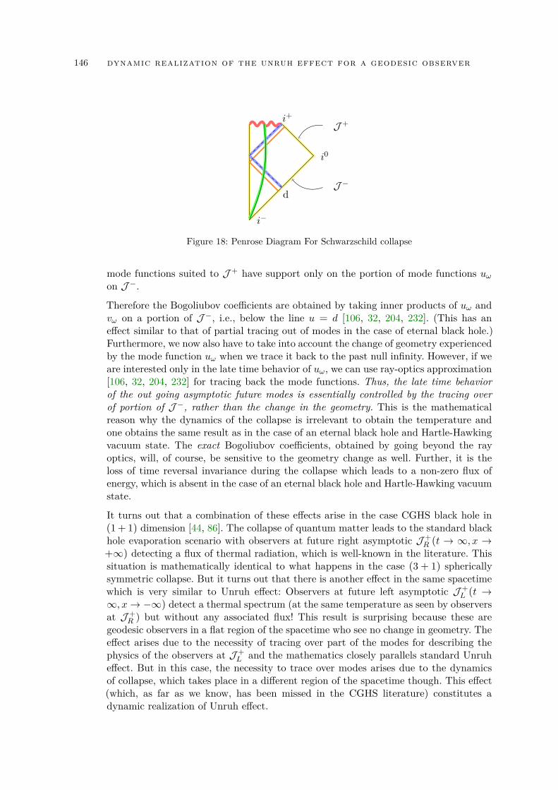
146 dynamic realization of the unruh effect for a geodesic observer

i+

i−

i0

d

J +

J −

Figure 18: Penrose Diagram For Schwarzschild collapse

mode functions suited to J + have support only on the portion of mode functions uωon J −.

Therefore the Bogoliubov coefficients are obtained by taking inner products of uω andvω on a portion of J −, i.e., below the line u = d [106, 32, 204, 232]. (This has aneffect similar to that of partial tracing out of modes in the case of eternal black hole.)Furthermore, we now also have to take into account the change of geometry experiencedby the mode function uω when we trace it back to the past null infinity. However, if weare interested only in the late time behavior of uω, we can use ray-optics approximation[106, 32, 204, 232] for tracing back the mode functions. Thus, the late time behaviorof the out going asymptotic future modes is essentially controlled by the tracing overof portion of J −, rather than the change in the geometry. This is the mathematicalreason why the dynamics of the collapse is irrelevant to obtain the temperature andone obtains the same result as in the case of an eternal black hole and Hartle-Hawkingvacuum state. The exact Bogoliubov coefficients, obtained by going beyond the rayoptics, will, of course, be sensitive to the geometry change as well. Further, it is theloss of time reversal invariance during the collapse which leads to a non-zero flux ofenergy, which is absent in the case of an eternal black hole and Hartle-Hawking vacuumstate.

It turns out that a combination of these effects arise in the case CGHS black hole in(1+ 1) dimension [44, 86]. The collapse of quantum matter leads to the standard blackhole evaporation scenario with observers at future right asymptotic J +

R (t → ∞,x →+∞) detecting a flux of thermal radiation, which is well-known in the literature. Thissituation is mathematically identical to what happens in the case (3 + 1) sphericallysymmetric collapse. But it turns out that there is another effect in the same spacetimewhich is very similar to Unruh effect: Observers at future left asymptotic J +

L (t →∞,x→ −∞) detect a thermal spectrum (at the same temperature as seen by observersat J +

R ) but without any associated flux! This result is surprising because these aregeodesic observers in a flat region of the spacetime who see no change in geometry. Theeffect arises due to the necessity of tracing over part of the modes for describing thephysics of the observers at J +

L and the mathematics closely parallels standard Unruheffect. But in this case, the necessity to trace over modes arises due to the dynamicsof collapse, which takes place in a different region of the spacetime though. This effect(which, as far as we know, has been missed in the CGHS literature) constitutes adynamic realization of Unruh effect.

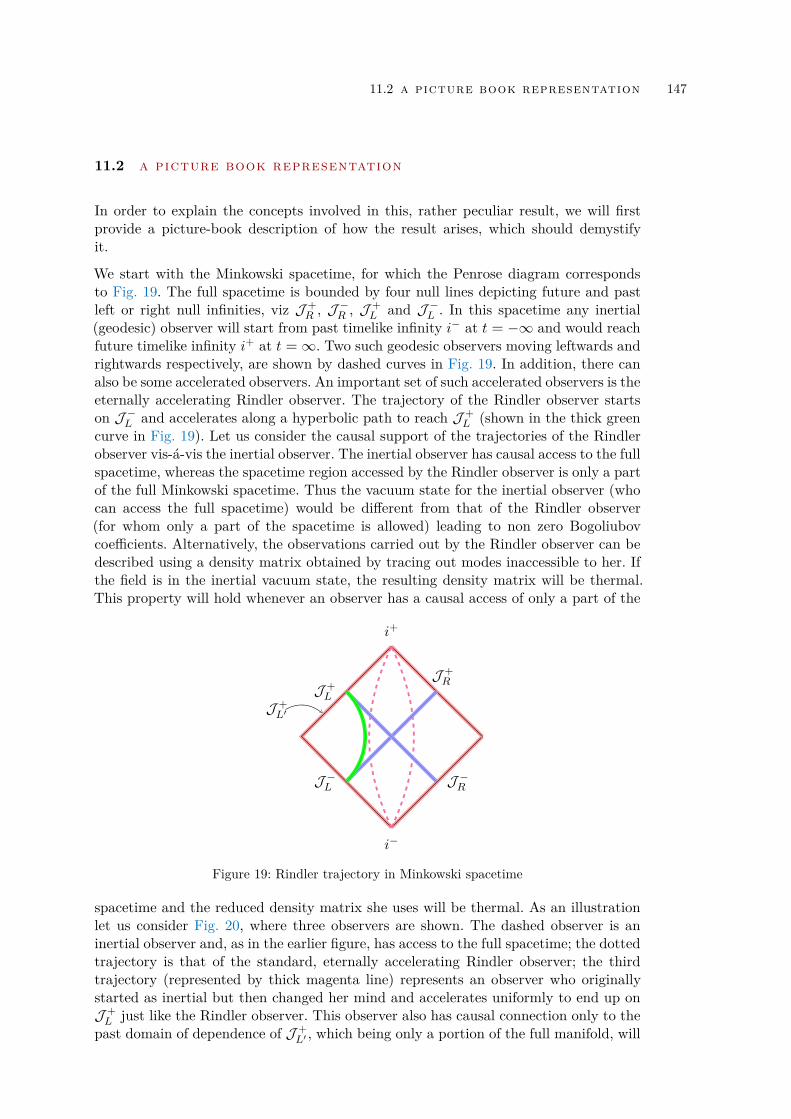
11.2 a picture book representation 147

11.2 a picture book representation

In order to explain the concepts involved in this, rather peculiar result, we will firstprovide a picture-book description of how the result arises, which should demystifyit.

We start with the Minkowski spacetime, for which the Penrose diagram correspondsto Fig. 19. The full spacetime is bounded by four null lines depicting future and pastleft or right null infinities, viz J +

R , J −R , J +L and J −L . In this spacetime any inertial

(geodesic) observer will start from past timelike infinity i− at t = −∞ and would reachfuture timelike infinity i+ at t =∞. Two such geodesic observers moving leftwards andrightwards respectively, are shown by dashed curves in Fig. 19. In addition, there canalso be some accelerated observers. An important set of such accelerated observers is theeternally accelerating Rindler observer. The trajectory of the Rindler observer startson J −L and accelerates along a hyperbolic path to reach J +

L (shown in the thick greencurve in Fig. 19). Let us consider the causal support of the trajectories of the Rindlerobserver vis-á-vis the inertial observer. The inertial observer has causal access to the fullspacetime, whereas the spacetime region accessed by the Rindler observer is only a partof the full Minkowski spacetime. Thus the vacuum state for the inertial observer (whocan access the full spacetime) would be different from that of the Rindler observer(for whom only a part of the spacetime is allowed) leading to non zero Bogoliubovcoefficients. Alternatively, the observations carried out by the Rindler observer can bedescribed using a density matrix obtained by tracing out modes inaccessible to her. Ifthe field is in the inertial vacuum state, the resulting density matrix will be thermal.This property will hold whenever an observer has a causal access of only a part of the

J +L′

J −R

J +L

J −L

J +R

i+

i−

Figure 19: Rindler trajectory in Minkowski spacetime

spacetime and the reduced density matrix she uses will be thermal. As an illustrationlet us consider Fig. 20, where three observers are shown. The dashed observer is aninertial observer and, as in the earlier figure, has access to the full spacetime; the dottedtrajectory is that of the standard, eternally accelerating Rindler observer; the thirdtrajectory (represented by thick magenta line) represents an observer who originallystarted as inertial but then changed her mind and accelerates uniformly to end up onJ +L just like the Rindler observer. This observer also has causal connection only to the

past domain of dependence of J +L′ , which being only a portion of the full manifold, will

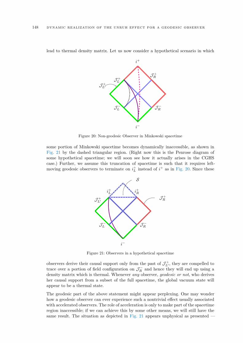
148 dynamic realization of the unruh effect for a geodesic observer

lead to thermal density matrix. Let us now consider a hypothetical scenario in which

J +L′

J −R

J +L

J −L

J +R

i+

i−

Figure 20: Non-geodesic Observer in Minkowski spacetime

some portion of Minkowski spacetime becomes dynamically inaccessible, as shown inFig. 21 by the dashed triangular region. (Right now this is the Penrose diagram ofsome hypothetical spacetime; we will soon see how it actually arises in the CGHScase.) Further, we assume this truncation of spacetime is such that it requires left-moving geodesic observers to terminate on i+L instead of i+ as in Fig. 20. Since these

J −R

S

J +RJ +

L′

J −L

i+R

i−

i+L

Figure 21: Observers in a hypothetical spacetime

observers derive their causal support only from the past of J +L′ , they are compelled to

trace over a portion of field configuration on J −R and hence they will end up using adensity matrix which is thermal. Whenever any observer, geodesic or not, who derivesher causal support from a subset of the full spacetime, the global vacuum state willappear to be a thermal state.

The geodesic part of the above statement might appear perplexing. One may wonderhow a geodesic observer can ever experience such a nontrivial effect usually associatedwith accelerated observers. The role of acceleration is only to make part of the spacetimeregion inaccessible; if we can achieve this by some other means, we will still have thesame result. The situation as depicted in Fig. 21 appears unphysical as presented —

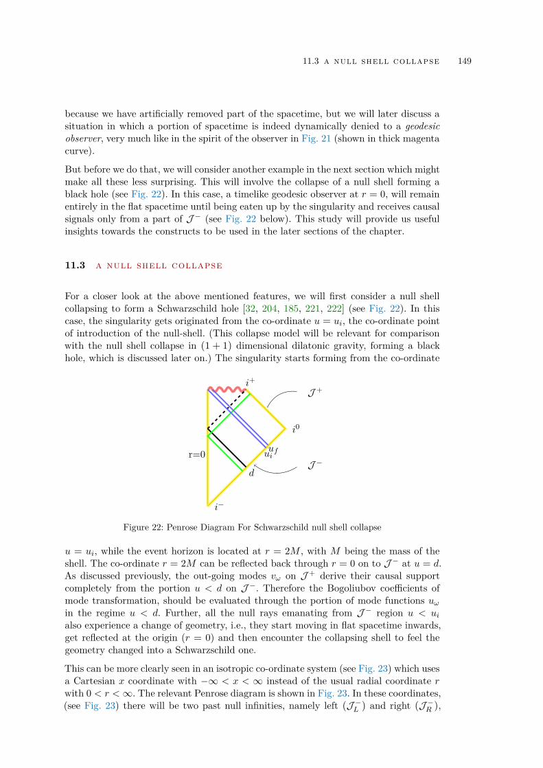
11.3 a null shell collapse 149

because we have artificially removed part of the spacetime, but we will later discuss asituation in which a portion of spacetime is indeed dynamically denied to a geodesicobserver, very much like in the spirit of the observer in Fig. 21 (shown in thick magentacurve).

But before we do that, we will consider another example in the next section which mightmake all these less surprising. This will involve the collapse of a null shell forming ablack hole (see Fig. 22). In this case, a timelike geodesic observer at r = 0, will remainentirely in the flat spacetime until being eaten up by the singularity and receives causalsignals only from a part of J − (see Fig. 22 below). This study will provide us usefulinsights towards the constructs to be used in the later sections of the chapter.

11.3 a null shell collapse

For a closer look at the above mentioned features, we will first consider a null shellcollapsing to form a Schwarzschild hole [32, 204, 185, 221, 222] (see Fig. 22). In thiscase, the singularity gets originated from the co-ordinate u = ui, the co-ordinate pointof introduction of the null-shell. (This collapse model will be relevant for comparisonwith the null shell collapse in (1 + 1) dimensional dilatonic gravity, forming a blackhole, which is discussed later on.) The singularity starts forming from the co-ordinate

i+

i−

i0

d

uiuf

J +

J −r=0

Figure 22: Penrose Diagram For Schwarzschild null shell collapse

u = ui, while the event horizon is located at r = 2M , with M being the mass of theshell. The co-ordinate r = 2M can be reflected back through r = 0 on to J − at u = d.As discussed previously, the out-going modes vω on J + derive their causal supportcompletely from the portion u < d on J −. Therefore the Bogoliubov coefficients ofmode transformation, should be evaluated through the portion of mode functions uωin the regime u < d. Further, all the null rays emanating from J − region u < uialso experience a change of geometry, i.e., they start moving in flat spacetime inwards,get reflected at the origin (r = 0) and then encounter the collapsing shell to feel thegeometry changed into a Schwarzschild one.

This can be more clearly seen in an isotropic co-ordinate system (see Fig. 23) which usesa Cartesian x coordinate with −∞ < x < ∞ instead of the usual radial coordinate rwith 0 < r <∞. The relevant Penrose diagram is shown in Fig. 23. In these coordinates,(see Fig. 23) there will be two past null infinities, namely left (J −L ) and right (J −R ),

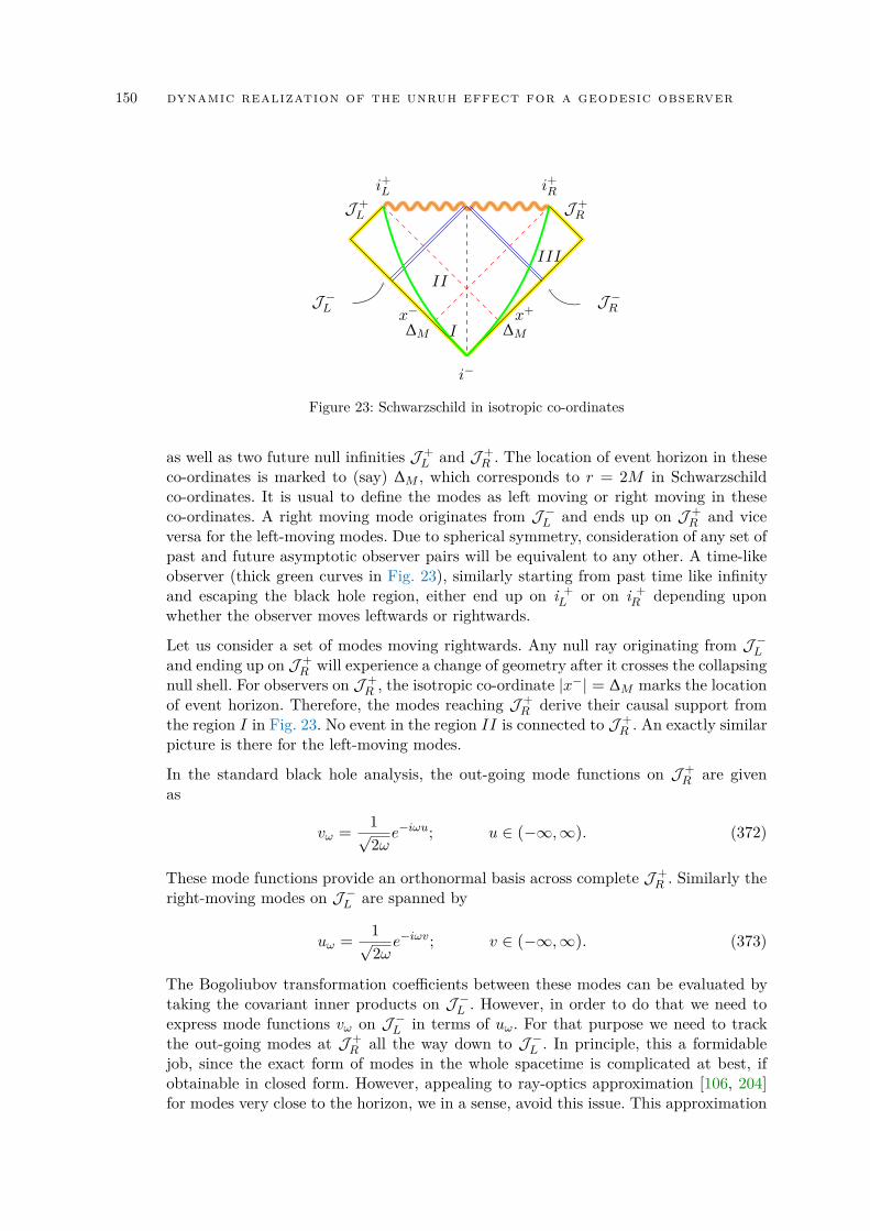
150 dynamic realization of the unruh effect for a geodesic observer

J +R

J −Rx−

J +L

J −Lx+

∆M ∆MI

II

III

i+L i+R

i−

Figure 23: Schwarzschild in isotropic co-ordinates

as well as two future null infinities J +L and J +

R . The location of event horizon in theseco-ordinates is marked to (say) ∆M , which corresponds to r = 2M in Schwarzschildco-ordinates. It is usual to define the modes as left moving or right moving in theseco-ordinates. A right moving mode originates from J −L and ends up on J +

R and viceversa for the left-moving modes. Due to spherical symmetry, consideration of any set ofpast and future asymptotic observer pairs will be equivalent to any other. A time-likeobserver (thick green curves in Fig. 23), similarly starting from past time like infinityand escaping the black hole region, either end up on i +

L or on i +R depending upon

whether the observer moves leftwards or rightwards.

Let us consider a set of modes moving rightwards. Any null ray originating from J −Land ending up on J +

R will experience a change of geometry after it crosses the collapsingnull shell. For observers on J +

R , the isotropic co-ordinate |x−| = ∆M marks the locationof event horizon. Therefore, the modes reaching J +

R derive their causal support fromthe region I in Fig. 23. No event in the region II is connected to J +

R . An exactly similarpicture is there for the left-moving modes.

In the standard black hole analysis, the out-going mode functions on J +R are given

as

vω =1√2ωe−iωu; u ∈ (−∞,∞). (372)

These mode functions provide an orthonormal basis across complete J +R . Similarly the

right-moving modes on J −L are spanned by

uω =1√2ωe−iωv; v ∈ (−∞,∞). (373)

The Bogoliubov transformation coefficients between these modes can be evaluated bytaking the covariant inner products on J −L . However, in order to do that we need toexpress mode functions vω on J −L in terms of uω. For that purpose we need to trackthe out-going modes at J +

R all the way down to J −L . In principle, this a formidablejob, since the exact form of modes in the whole spacetime is complicated at best, ifobtainable in closed form. However, appealing to ray-optics approximation [106, 204]for modes very close to the horizon, we in a sense, avoid this issue. This approximation

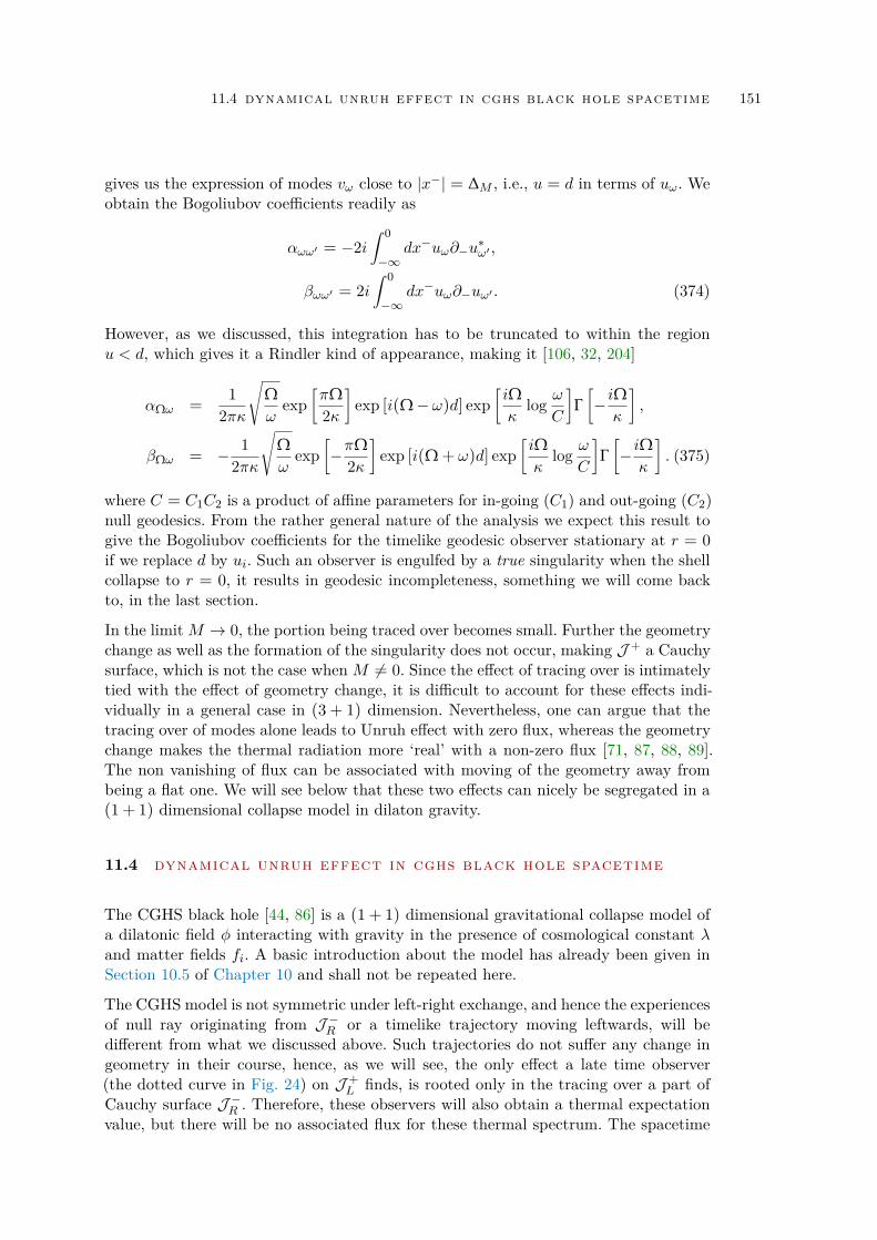
11.4 dynamical unruh effect in cghs black hole spacetime 151

gives us the expression of modes vω close to |x−| = ∆M , i.e., u = d in terms of uω. Weobtain the Bogoliubov coefficients readily as

αωω′ = −2i∫ 0

−∞dx−uω∂−u

∗ω′ ,

βωω′ = 2i∫ 0

−∞dx−uω∂−uω′ . (374)

However, as we discussed, this integration has to be truncated to within the regionu < d, which gives it a Rindler kind of appearance, making it [106, 32, 204]

αΩω =1

2πκ

√Ωω

exp[πΩ2κ

]exp [i(Ω− ω)d] exp

[iΩκ

log ωC

]Γ[− iΩκ

],

βΩω = − 12πκ

√Ωω

exp[−πΩ

2κ

]exp [i(Ω + ω)d] exp

[iΩκ

log ωC

]Γ[− iΩκ

]. (375)

where C = C1C2 is a product of affine parameters for in-going (C1) and out-going (C2)null geodesics. From the rather general nature of the analysis we expect this result togive the Bogoliubov coefficients for the timelike geodesic observer stationary at r = 0if we replace d by ui. Such an observer is engulfed by a true singularity when the shellcollapse to r = 0, it results in geodesic incompleteness, something we will come backto, in the last section.

In the limitM → 0, the portion being traced over becomes small. Further the geometrychange as well as the formation of the singularity does not occur, making J + a Cauchysurface, which is not the case whenM 6= 0. Since the effect of tracing over is intimatelytied with the effect of geometry change, it is difficult to account for these effects indi-vidually in a general case in (3 + 1) dimension. Nevertheless, one can argue that thetracing over of modes alone leads to Unruh effect with zero flux, whereas the geometrychange makes the thermal radiation more ‘real’ with a non-zero flux [71, 87, 88, 89].The non vanishing of flux can be associated with moving of the geometry away frombeing a flat one. We will see below that these two effects can nicely be segregated in a(1 + 1) dimensional collapse model in dilaton gravity.

11.4 dynamical unruh effect in cghs black hole spacetime

The CGHS black hole [44, 86] is a (1 + 1) dimensional gravitational collapse model ofa dilatonic field φ interacting with gravity in the presence of cosmological constant λand matter fields fi. A basic introduction about the model has already been given inSection 10.5 of Chapter 10 and shall not be repeated here.

The CGHS model is not symmetric under left-right exchange, and hence the experiencesof null ray originating from J −R or a timelike trajectory moving leftwards, will bedifferent from what we discussed above. Such trajectories do not suffer any change ingeometry in their course, hence, as we will see, the only effect a late time observer(the dotted curve in Fig. 24) on J +

L finds, is rooted only in the tracing over a part ofCauchy surface J −R . Therefore, these observers will also obtain a thermal expectationvalue, but there will be no associated flux for these thermal spectrum. The spacetime

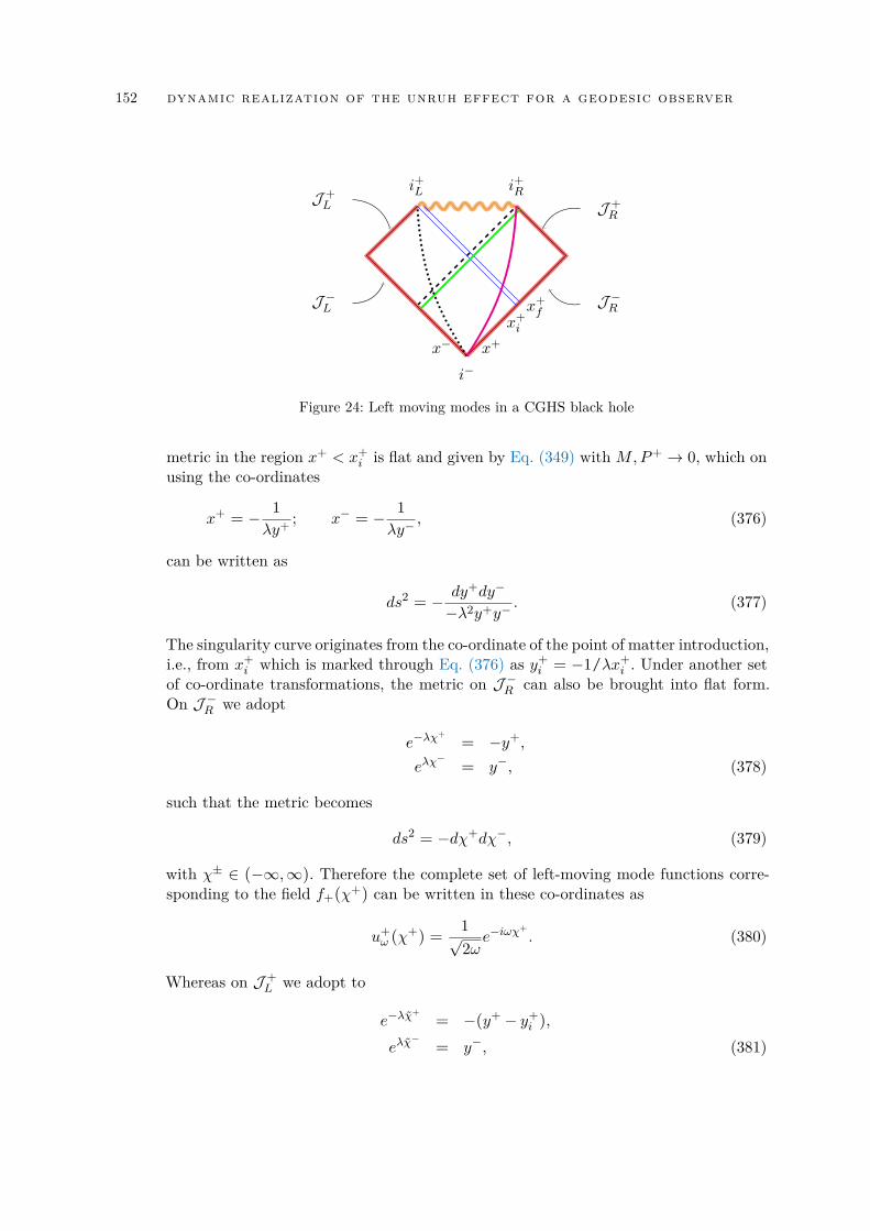
152 dynamic realization of the unruh effect for a geodesic observer

J +R

J −Rx+i

x−

J +L

J −L x+f

x+

i+L i+R

i−

Figure 24: Left moving modes in a CGHS black hole

metric in the region x+ < x+i is flat and given by Eq. (349) with M ,P+ → 0, which onusing the co-ordinates

x+ = − 1λy+

; x− = − 1λy−

, (376)

can be written as

ds2 = − dy+dy−

−λ2y+y−. (377)

The singularity curve originates from the co-ordinate of the point of matter introduction,i.e., from x+i which is marked through Eq. (376) as y+i = −1/λx+i . Under another setof co-ordinate transformations, the metric on J −R can also be brought into flat form.On J −R we adopt

e−λχ+

= −y+,eλχ

−= y−, (378)

such that the metric becomes

ds2 = −dχ+dχ−, (379)

with χ± ∈ (−∞,∞). Therefore the complete set of left-moving mode functions corre-sponding to the field f+(χ+) can be written in these co-ordinates as

u+ω (χ+) =

1√2ωe−iωχ

+ . (380)

Whereas on J +L we adopt to

e−λχ+

= −(y+ − y+i ),eλχ

−= y−, (381)

11.4 dynamical unruh effect in cghs black hole spacetime 153

such that these new co-ordinates range in χ± ∈ (−∞,∞) in the region x+ < x+i . Themetric in these new co-ordinates becomes

ds2 = − dχ+dχ−

1− y+i eλχ+ . (382)

The metric Eq. (382) is in a conformally flat form in these co-ordinates, hence thecomplete set of left-moving modes corresponding to f+(χ+) are again given as

v+ω (χ+) =

1√2ωe−iωχ

+ , (383)

since a minimally coupled scalar field is conformally invariant in (1 + 1) dimensions.Clearly, on J −R , v+ω has support only in the region x+ < x+i . The point x+i is mappedto χ+ ≡ χ+i = − 1

λ log (−y+i ). Therefore, the Bogoliubov transformation coefficientsbetween these two set of observers can be obtained exactly as in Eq. (362), Eq. (363)but with the replacement |y+i | ↔ P+/λ as

αΩω = − iπ

∫ χ+i

−∞dχ+vΩ∂−u

∗ω

=1

2π

√ω

Ω

∫ χ+i

−∞dχ+ exp

[iΩλ

ln(e−λχ

+ − |y+i |)

+ iωχ+]

=1

2πλ

√ω

Ω|y+i |

i(Ω−ω)λ B

(− iΩλ

+iω

λ, 1 + iΩ

λ

), (384)

while

βΩω =i

π

∫ χ+i

−∞dχ+vΩ∂+uω

=1

2π

√ω

Ω

∫ χ+i

−∞dχ+ exp

[iΩλ

ln(e−λχ

+ − |y+i |)− iωχ+

]=

12πλ

√ω

Ω|y+i |

i(Ω+ω)λ B

(− iΩλ− iω

λ, 1 + iΩ

λ

). (385)

This form of Bogoliubov coefficients results from the tracing over of a portion of J −R ,which is causally disconnected from J +

L . The horizon for J +L is given as y+ = y+i ,

which also marks the point of singularity. More importantly, if one is interested in thelate time response, i.e., the observers reaching i+L , we need to take the high frequencybehavior (ω/λ 1) of the Bogoliubov coefficients which are exactly the same as forthe Rindler observer [167].

This effect can be more clearly understood using non-availability of Cauchy surfacesfor future asymptotic observers. Let us consider a left moving timelike or null tra-jectory. Due to conformal flatness, a complete set of orthonormal mode functions onany surface orthogonal to them, can always be obtained as plane waves under a properco-ordinatization (which extends as (−∞,∞)) of that surface. If we consider an orthog-onal null surface for the left moving modes, before the formation of singularity (thered surface labeled ‘2’ in Fig. 25), the Bogoliubov transformation coefficients betweenthat surface and J −R will be trivial, i.e., (αΩω = δ(Ω− ω),βΩω = 0). However, oncethe singularity forms, any null surface relating a point on J −L to the singularity (e.g.,green surface labeled ‘1’ in Fig. 25), fails to causally connect with the entire spacetime.

154 dynamic realization of the unruh effect for a geodesic observer

J +R

J −Rx+i

x−

J +L

J −L x+f

x+

i+L i+R

i−

1 2

Figure 25: Unavailability of Cauchy surface for left-moving modes

Also, any timelike observer has a domain of dependence, which is not the full space-time. A portion of J −R (right to the dashed green line) is causally denied to the pastof such surfaces. Therefore, the Bogoliubov coefficients assume a non-trivial form, suchas in Eq. (362), Eq. (363) or Eq. (384), Eq. (385), with a phase factor capturing theinformation about the region of the traced over modes. This is dynamically similar to aRindler trajectory in a Minkowski spacetime, see Fig. 19, where an accelerated observer(thick green curve) reaches the future null infinity rather than future timelike infinity.For such observers too, the domain of dependence is only a part of the full spacetime.There is a horizon masking a portion of spacetime and hence the Bogoliubov trans-formation coefficients between J −R and J +

L′ (rather than the full J +L ) is non-trivial

[232, 32, 167] and the accelerated observers obtain a thermal spectrum for a vacuumstate defined on J −R . However, there is no flux associated with this spectrum as thestress tensor remains identically vanishing in the flat spacetime.

Similarly in the CGHS model, the region of spacetime y+ > y+i is dynamically madeinaccessible to any left-moving time-like or null trajectories, which also is the casewith such trajectories in the null collapse forming a Schwarzschild black hole (see forexample, Fig. 23). However, in contrast to the Schwarzschild case, such observers in theCGHS model, do not see any change of geometry hence they do not associate any massto the “black hole region” as seen by them. The spacetime, they move in, throughout, isflat and such observers do not receive any flux of radiation, as the vacuum expectationvalue of the stress energy tensor which was vanishing on J −R , stays put on zero, inthe region y+ < y+i . As we discussed previously, the right moving observers tuned toright moving modes, witness a thermal radiation flux at a temperature 1/λ which isindependent of the matter content of the forming black hole and depends only on theother dimensionful parameter in the theory.

Similarly, the observers at J +L coupled to left-moving modes, observe a similar kind of

Bogoliubov coefficients as their right-moving counterparts Eq. (362), Eq. (363) but withthe parameter exchange |y+i | ↔ P+/λ which mark the corresponding event horizons forsuch observers and appear as overall phases in the transformation coefficients. Hence,we see that such form of Bogoliubov coefficients Eq. (384), Eq. (385) are entirely dueto tracing over of modes which lie in the causally denied region of spacetime, to I+Land not due to any geometry change. One can check that if the fraction of tracing overvanishes, which is marked by |y+i | → 0, the Bogoliubov coefficients assume a trivialform, i.e., αΩω → δ(Ω− ω) while βΩω → 0. Similarly, the Bogoliubov coefficients for

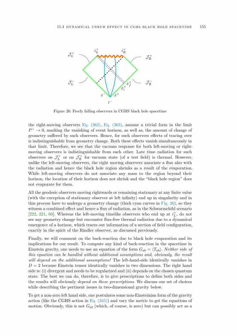
11.4 dynamical unruh effect in cghs black hole spacetime 155

J +R

J −Rx+i

x−

J +L

J −L x+f

x+

i+L i+R

i−

Figure 26: Freely falling observers in CGHS black hole spacetime

the right-moving observers Eq. (362), Eq. (363), assume a trivial form in the limitP+ → 0, marking the vanishing of event horizon, as well as, the amount of change ofgeometry suffered by such observers. Hence, for such observers effects of tracing overis indistinguishable from geometry change. Both these effects vanish simultaneously inthat limit. Therefore, we see that the vacuum response for both left-moving or right-moving observers is indistinguishable from each other. Late time radiation for suchobservers on J +

L or on J +R for vacuum state (of a test field) is thermal. However,

unlike the left-moving observers, the right moving observers associate a flux also withthe radiation and hence the black hole region shrinks as a result of the evaporation.While left-moving observers do not associate any mass to the region beyond theirhorizon, the location of their horizon does not shrink and the “black hole region” doesnot evaporate for them.

All the geodesic observers moving rightwards or remaining stationary at any finite value(with the exception of stationary observer at left infinity) end up in singularity and inthis process have to undergo a geometry change (thick cyan curves in Fig. 26), so theywitness a combined effect and hence a flux of radiation, as in the Schwarzschild scenario[222, 221, 60]. Whereas the left-moving timelike observers who end up at i+L , do notsee any geometry change but encounter flux-free thermal radiation due to a dynamicalemergence of a horizon, which traces out information of a section of field configuration,exactly in the spirit of the Rindler observer, as discussed previously.

Finally, we will comment on the back-reaction due to black hole evaporation and itsimplications for our result. To compute any kind of back-reaction in the spacetime inEinstein gravity, one needs to use an equation of the form Gab = 〈Tab〉. Neither side ofthis equation can be handled without additional assumptions and, obviously, the resultwill depend on the additional assumptions! The left-hand-side identically vanishes inD = 2 because Einstein tensor identically vanishes in two dimensions. The right handside is: (i) divergent and needs to be regularized and (ii) depends on the chosen quantumstate. The best we can do, therefore, is to give prescriptions to define both sides andthe results will obviously depend on these prescriptions. We discuss our set of choiceswhile describing the pertinent issues in two-dimensional gravity below.

To get a non-zero left hand side, one postulates some non-Einsteinian form of the gravityaction (like the CGHS action in Eq. (345)) and vary the metric to get the equations ofmotion. Obviously, this is not Gab (which, of course, is zero) but can possibly act as a

156 dynamic realization of the unruh effect for a geodesic observer

proxy for the same. We stress the fact that we are trying to model some gravitationalfeatures by some suitable dilatonic action and one cannot ignore the implicit ad-hocnessin the procedure. For example, in such an approach, one also often takes the normalordered, non-covariant, expectation value of the stress energy tensor as the classicalsource. However, in a two-dimensional spacetime, the expectation value of the stressenergy tensor comes with a conformal anomaly term [86] as well. The anomaly term canthen act as an extra source of stress energy and may lead to an evolution different fromthe classical case, if not accounted for properly. A prescription used in the literatureis to add some extra terms (e.g., Polyakov action, RST action terms) to the standardCGHS action corresponding to the conformal anomaly terms and obtain these modifiedequations of motion, as a result of the variational principle. But this new action willcorrespond to a different physical system, though one which can also be thought of asa proxy for gravity. But in this prescription, flat spacetime will not be a solution tothe vacuum state for the semiclassical equations due to the anomaly, which we considersomewhat unphysical. There is no unique way of handling this issue because, as westressed before, Gab = 0 in D = 2 and the left hand side which we work with to mimicGab = 〈Tab〉 depends crucially on the model we use, with the hope that it can mimicaspects of D = 4 gravity. We have chosen simple, physically well-motivated choices todo this as we describe next.

To analyze the right hand side, we need a scheme for defining a c−number stress tensorfrom the quantum operator and the vacuum state has to be motivated from somespecific (geometric) considerations. We have defined the vacuum state by a naturalassumption: viz. that the geometry must remain flat when sourced by such a (vacuum)state. This is important because as we discussed, in two-dimensional spacetime, theexpectation value of the stress energy tensor has a conformal anomaly term which canviolate this criterion in general, if this term is not accounted for in the source termsin the right hand side. However, there exists a family of such states [144] which takecare of the conformal anomaly terms and ensure that the geometry remains flat whenthe state is a vacuum from this family. Therefore the results discussed in this chapter,use stability of the solution under these class of states. A more detailed analysis ofconformal anomaly modified evaporating black holes can be found in [86]. Our schemeto deal with such terms will be reported in details elsewhere [145]. At last, we discussthe response of an Unruh-DeWitt detector carried by such a geodesic observer.

11.5 unruh-dewitt detector response

To confirm the fact operationally, that an observer who entirely stays in the left blockof spacetime and has access to only a portion of full spacetime, truly finds the vacuumstate of a field defined/supported in the full spacetime as an excited state on herHilbert space defined in the portion of spacetime, we turn to analysis of response of anUnruh-DeWitt detector carried by a left-moving inertial observer.

Such an observer describes the spacetime metric as in Eq. (379). We construct a co-ordinate system x ≡ (T ,X)

χ+ = T +X

χ− = T −X (386)

11.5 unruh-dewitt detector response 157

to write Eq. (379) as

ds2 = −dT 2 + dX2 (387)

such that the Wightman function, corresponding to the vacuum defined in full space-time, in (1 + 1) dimension assumes the form

W(x,x′) = −12 log |x− x′|2 = −1

2 log ∆χ+∆χ−. (388)

A left moving inertial observer is given by the trajectory

dT

dτ= γ; dX

dτ= −vγ,

where v is the inertial velocity and γ is the corresponding Lorentz factor. If the space-time were flat throughout, i.e., no matter shell had collapsed, the inertial observer, car-rying the detector, would have exhausted the full range of proper time τ ∈ (−∞,∞).The appearance of singularity due to collapse of the matter shell leads to geodesic in-completeness and hence regulate the proper time interval of the geodesic observer to(−∞, τf ), with τf marking the location i+L (see the left curve in Fig. 25).

In (1+ 1) dimension, the response of a monopole detector coupled to a (test) field Φ(x)is ambiguous [148]. Therefore, we work with derivative field detector with interactionHamiltonian

Hint = cµ(τ )d

dτΦ(x(τ )), (389)

where c is a coupling constant, µ(τ ) is detector’s monopole moment operator and τis the proper time detected by observer carrying the detector. The detector responsefunction [148], for a two level detector, with level separation ω, will be given for thiscase as

F (1)(ω) =∫ τf

−∞dτ

∫ τf

−∞dτ ′e−iω(τ−τ

′)∂τ∂τ ′W(τ , τ ′). (390)

In flat portion of the spacetime, on any trajectory, if the test field Φ(x) is in the vacuumstate,

∂τ∂τ ′W(τ , τ ′) = 1(τ − τ ′)2 , (391)

becomes solely a function of ∆τ = τ − τ ′. Had the spacetime been geodesically complete,τf → ∞ and the detector would not have clicked. However, due to collapsing matterfield and the subsequent removal of a portion of spacetime, the spacetime becomesgeodesically incomplete. In such a case, the detector response will be analogous to afinite time inertial detector [225], which indeed registers clicks. However, notice thathere we have not introduced any artificial switching function, but it is the inextendibilityof the geodesic, which leads to the non-zero response function. In the case there is noblack hole collapse, the detector will fall silent.

158 dynamic realization of the unruh effect for a geodesic observer

We can now transform to co-ordinates ∆τ and a mean proper time τ = (τ + τ ′)/2 tore-write Eq. (390) as

F (1)(ω) =∫ τf

−∞dτ

∫ (2τf−2τ )

−(2τf−2τ )

d∆τ(∆τ )2 e

−iω∆τ . (392)

Therefore, the detection rate becomes time dependent as fit for a detector movingthrough an excited state [146], i.e., at different points on the trajectory the detectorwill click differently. Hence, we show that the detector also conforms to the notion thatthe state as measured by the left moving geodesic observer is non-vacuum. With a bitof exercise [225], one can evaluate the clicking rate of the detector at any general pointof time as well. The detector clicks with a non-zero rate and the left-moving observerconcludes that there are particles in her patch of the spacetime.

It is important to note that this detector is constructed in a manner such that itwill not register any clicking, if the quantum field resides in the vacuum state of theobserver carrying the detector along (e.g., Inertial observer in Minkowski spacetimein regular (3 + 1) dimensional gravity). Therefore, the global vacuum defined on J −Rfails to be a vacuum state for left-moving geodesic observers. Further, the detectordoes not click in a steady fashion at a thermal detection rate, but this is due to thefact that the detector response depends hugely on the trajectory unlike the Bogoliubovtransformation. For instance, it is easy to demonstrate that in Fig. 20 the non-geodesicobserver (thick magenta curve) and the Rindler observer (dotted trajectory) obtain thesame Bogoliubov coefficients as they derive the casual support from the same patch, yetUnruh-DeWitt detectors carried by them behave differently. Still both such observersagree that the state they measure is non-vacuum.

Part V

ZERO POINT LENGTH — TOWARDS QUANTUMGRAVITY

12SPACETIME WITH ZERO POINT LENGTH ISTWO-D IMENS IONAL AT THE PLANCK SCALE

12.1 introduction and motivation

The existence of a fundamental length scale, which provides an ultimate lower bound tomeasurement of spacetime intervals, is a model-independent feature of quantum gravity,since various approaches to quantum gravity lead to this result. The appearance of sucha minimum length scale actually derives from basic principles of quantum mechanics,special and general relativity, and hence is often considered as a robust feature ofquantum gravity. This result can have important consequences, e.g., notions of causalityor distance between two events cannot be expected to have a continuous behaviour atthis length scale [74, 173, 172, 174, 94, 93].

It seems, therefore, natural to look for a description of spacetime at the mesoscopicscales which interpolate between Planck scale and low energy scales, by incorporatingthe effect of introducing a zero point length to the spacetime through modificationof the spacetime metric gab to some suitable object qab, which we shall refer to asthe qmetric. The qab must be constructed such that the geodesic distance betweentwo points computed using qab acquires a lower bound [135]. If we can determine theqmetric in terms of gab, then we can compute all other geometrical variables (like,for e.g., curvature tensor) by using the qmetric in the place of gab in the relevantexpressions. Such a procedure is necessarily approximate — compared to a fully rigorousnon-perturbative quantum gravitational approach — but will surely capture some ofthe effects at the mesoscopic scales which interpolate between Planck scale and lowenergy scales at which the classical metric provides an adequate description.

Unfortunately, we cannot use perturbation techniques to compute qab for a given classi-cal geometry described by a gab. In fact, we would expect it to be non-local and singularat any given event. In the absence of explicit computability, we need a physically moti-vated ansatz to relate qab to gab. Such an ansatz was introduced and described in fairdetail in [135]. The essential idea was to recognize that a primary effect of quantumgravity will be to endow spacetime with a zero-point length [74, 173, 172, 174, 94, 93]by modifying the geodesic interval σ2(x,x′) between two events x and x′ in a Euclideanspacetime to a form like σ2 → σ2 + `20 (here `0 ∼ LP , the Planck length). More gen-erally, we will assume that a key effect of quantum gravity is to modify σ2 → F(σ2)where the function F(σ2) satisfies the constraint F(0) = `20. While most of our resultsare insensitive to the explicit functional form of F(σ2), for illustration, we will useF(σ2) = σ2 + `20.

This approach essentially treats the σ2(x,x′) as more fundamental than the metricgab(x) itself. As we have already emphasized, there is considerable amount of evidencefor the existence of such a zero-point-length of spacetime; there have also been argu-ments in the literature suggesting that gab may not be the most primitive variable to

161

162 spacetime with zero point length is two-dimensional at the planck scale

use while studying quantum gravitational effects (see e.g., [114]). The key claim being,while we may not know how quantum gravity modifies the classical metric a priori,we do have an indirect handle on it, if we assume that quantum gravity introduces azero-point length to the spacetime in the manner described above.

One can determine [133, 226] the form of qab for a given gab by using the requirementsthat

1. It should lead to a spacetime interval with a zero-point-length.

2. The two-point function describing small perturbations of the metric should havea regularized non-singular coincidence limit.

It was shown in the earlier works [133, 226] that these conditions allow us to determineqab uniquely in terms of gab (and its associated geodesic interval σ2). We find that

qab = Ahab +Bnanb; qab =1Ahab +

1Bnanb (393)

where hab = gab − nanb, and

B =σ2

σ2 + `20; A =

(∆∆F

)2/D1 σ2 + `20σ2 ; na =

∇aσ2

2√σ2

(394)

with ∆ being the Van Vleck determinant related to the geodesic interval σ2 by

∆(x,x′) = 1√g(x)g(x′)

det1

2∇xa∇x

′b σ

2(x,x′)

(395)

∆F is defined by replacing σ2 with F(σ2) in the series expansion of ∆ (see [226]). We in-terpret qab as the effective spacetime metric incorporating some of the non-perturbativeeffects of quantum gravity at Planck scales. As described in detail in the previous works[135, 136] the qmetric has the following properties:

• Unlike gab(x), the qmetric qab(x,x′) is a bi-tensor depending on two events x,x′through σ2. It is easy to show that this non-locality is essential if spacetime hasto acquire a zero-point length. Almost by definition, any local metric will lead toa geodesic interval which vanishes in the limit of x→ x′.

• qab reduces to the background metric gab in the limit of `20 → 0. That is, in theclassical limit of h → 0, qmetric reduces to the standard metric as we wouldexpect.

• In the opposite limit of (σ2/`20)→ 0 the qmetric is singular at all events. This isnatural when we interpret qmetric as the metric of the mesoscopic spacetime; wewould not expect it to be well defined at any given event and will require somekind of smearing over Planck scales for it to be meaningful.

• If the background metric is flat, then the qmetric is also flat, i.e., there exists acoordinate mapping from qab → ηab. This is, however, rather subtle because thecoordinate transformation is, in fact, singular in the coincidence limit in (regular)Cartesian coordinates, and the mapping effectively removes a geodesic region ofsize `0 from the spacetime around all events.

12.2 volume and area in presence of zero point length 163

• Let Φ[gab(x)] be a scalar constructed from the background metric and possiblyseveral of its derivatives, like, for example, the Ricci scalar R[gab(x)].

We can now compute the corresponding (bi)scalar Φ[qab(x,x′); `20] for the qmetric byreplacing gab by qab in Φ[gab(x)] and evaluating all derivatives at x keeping x′ (“basepoint”) fixed. We interpret the value of this scalar by taking the limit x → x′ in thisexpression keeping `20 non-zero. As noted in [135, 136], several useful scalars like R, Ketc. remain finite and local in this limit even though the qmetric itself is singular whenx → x′ with non-zero `20. This arises from the algebraic fact that the following twolimits do not commute:

lim`20→0

limx→x′

Φ[qab(x,x′); `20] 6= limx→x′

lim`20→0

Φ[qab(x,x′); `20] (396)

All these computations are most easily performed [58] by choosing a synchronous co-ordinate system for the background metric which can always be done in a local region.In this coordinate system, the equi-geodesic surface σ = constant, which is at a con-stant geodesic distance from the base point, has a simple description. These facts showthat we have a well-defined procedure for doing the computations in the mesoscopicspacetimes using the qmetric. More details regarding this approach will be presentedelsewhere [58].

12.2 volume and area in presence of zero point length

In this chapter, we will concentrate on one key effect of introducing such a zero pointlength to the spacetime metric. This relates to the volume of the geodesic ball:

VD(`, `0) ≡∫σ≤`

dσdΩD−1√q (397)

enclosed by an equi-geodesic surface of size σ = ` in the D-dimensional Euclideanspacetime. Here, q is the determinant of the qmetric with

√q =

(∆∆F

)(σ2 + `20σ2

)D2/2√g; D2 ≡ (D− 2) (398)

Classically we would expect the scaling VD(`) ∝ `D for sufficiently small ` when we canignore the scales involved in spacetime curvature. Let us now evaluate the same quantityfor the mesoscopic spacetime. Using the synchronous coordinates, a straightforward(though lengthy) calculation, gives the following result:

√q = σ

(σ2 + `20

)D2/2(

1− 16S(x

′)(σ2 + `20

)+ · · ·

)(399)

where S ≡ Rabnanb is a scalar constructed from the background gab and is evaluated

at base point x′. (Though we only need the leading order term, we have displayed nextorder term in the expansion which contribute in the limit of `20/σ2 → 0.) Here na isthe tangent to the geodesic and hence depends on the geodesic that connects the basepoint x′ to the point x on the equi-geodesic surface. Thus integrating over the angularcoordinates on the equi-geodesic surface amounts to averaging na over the solid angle.

164 spacetime with zero point length is two-dimensional at the planck scale

[Such an angular integral over nanb leads to, (Ω/D)gab, where Ω = 2πD/2Γ(D/2)−1

(see e.g., [100])]. A straightforward integration now gives the result, to the same orderof accuracy, as:

VD(`, `0) =ΩD

(`2 + `20

)D/2− `D0

− Ω

6D(D+ 2)R(x′)

(`2 + `20

)(D+2)/2− `D+2

0

(400)

where R is the Ricci scalar for the background metric gab.

Let us now consider the two relevant limits of this expression. First, when (`0/`)→ 0,we get

lim`0→0

VD(`, `0) =ΩD`D[1− 1

6(D+ 2)R(x′)`2

](401)

which shows that the volume scales as `D except for curvature induced correctionscaptured by the second term. This correction is a standard result known in differentialgeometry [100]. What is more interesting is the limit of (`/`0)→ 0, when we get

lim`→0

VD(`, `0) =Ω2 `

D0

(`2

`20

)[1− 1

6DR(x′)`20

]→ Ω

2 `D0

(`2

`20

)∝ `2 (402)

This suggests the remarkable possibility that the existence of zero-point-length makesthe physical spacetime essentially 2-dimensional near Planck scale. A convenient mea-sure of such a dimensional reduction is provided by the quantity

Deff = D+d

d ln `

ln(

VD(`, `0)VD(`, `0 = 0)

)(403)

which, using the above expressions, decreases from Deff = D for large ` to Deff = 2as ` → 0. It might seem that a simpler definition is just Deff = (d lnVD(`, `0)/d ln `).However, in any D-dimensional curved space with a smooth metric gab, this definitionwill give D only for R`2 1; that is at scales small compared to curvature scale. Therole of VD(`, `0 = 0) in the definition is to remove the contribution from the backgroundcurvature to Deff thereby ensuring that Deff = D when `0 = 0. So any deviation of Dfrom Deff arises only due to the existence of the zero-point-length.

There have been several indications from various approaches to quantum gravity thatspacetime might “look” two dimensional when probed at extremely small scales (mostof these arguments refer to the so called spectral dimension defined via the process ofrandom walk). Carlip [52, 50, 49, 41] has given several independent set of argumentssuggesting that such a dimensional reduction may be an inevitable feature of quantumgravity. Somewhat closer in spirit to the ideas presented here seems to be the results of[11, 10], where the authors argue that dimensional reduction to D = 2 might providea mechanism by which quantum gravity “self-renormalizes” at Planck scale. A geo-metrically similar approach (but based on quantization of area) in the context of loopquantum gravity and spin-foam models, was discussed in [164, 42, 43], while similarresult was obtained in the context of generalized uncertainty principle in [120]. Thecurrent study links such a dimensional reduction to the existence of zero-point-lengthin spacetime, independent of any specific model of quantum gravity.

12.3 conclusions 165

To understand the algebraic origin of this result, one could study the case of a flatspacetime in synchronous coordinates in which σ denotes the radial geodesic distancefrom a chosen origin. In this case, the qmetric leads to the line element of the form(when D = 4)

ds2 =1

A(σ)dσ2 +A(σ)σ2dΩ2

3; A = 1 + `20σ2 (404)

which transforms to ds2 = dσ2 + σ2dΩ23 with σ =

√σ2 + `20. In regular Cartesian coor-

dinates, this transformation is singular in the coincidence limit (see Appendix A of [133])and is equivalent to removing a “hole” of radius `0 from the manifold in a specific man-ner. In fact, in flat spacetime, we will get the result VD(`, `0) = (Ω/D)[

(`2 + `20

)D/2−`D0 ] which clearly has the limits VD(`, `0) ∝ `D (when (`0/`) → 0) and VD(`, `0) ∝ `2

(when (`/`0)→ 0). This clarifies the algebraic origin of the result.

12.3 conclusions

We believe the conjecture, that the mesoscopic spacetime is described by the qmetric, isa powerful and useful one. It is well motivated by the existence of the zero-point-lengthin the spacetime and leads to well defined computation rules which can incorporatethe effects of quantum gravity at mesoscopic scales without us leaving the comfort of acontinuum differential geometry (albeit one involving a singular and non-local metric).Its power is seen once again in the current chapter, where it leads to a definite conclusionthat the effective dimensionality of the spacetime at Planck scales is Deff = 2. Thisopens up useful further avenues of exploration.

Part VI

SUMMARY AND OUTLOOK

13SUMMARY AND OUTLOOK

In this last chapter, we shall present a concise summary of the results we have obtainedin this thesis as well as future directions of exploration.

As emphasized in the introduction, general relativity is the strongest candidate for de-scribing gravity and has passed all the experimental tests, starting from bending oflight in 1920 to detection of gravitational waves in 2015, with flying colors. Despiteits outstanding successes general relativity is not a complete theory. This has to dowith two facts — (i) general relativity leads to existence of singularities, where pre-dictability, essential for being a complete theory, breaks down and (ii) being a classicaltheory it cannot explain the universe at sufficiently small length scales (equivalently atsufficiently high energies). It is often postulated that the two issues are interrelated, assoon as one has a “quantum theory of gravity” one would achieve a possible resolutionof singularity. There are many candidates for the yet-to-be-built theory of quantumgravity, but they all lack in one perspective or another and no unique description hasemerged till date.

This motivates a fresh look at the problem, which started after Bekenstein and Hawkingdiscovered that one can associate an entropy and a temperature [27, 106] with blackholes. Soon after it was shown that black holes obey the laws of thermodynamicsas well [107, 23]. In 1995, Jacobson was able to show that, starting from Clausiusrelation one can arrive at Einstein’s field equations [122], which was complementedin 2002 by Padmanabhan, who showed that Einstein’s equations can be written in athermodynamic language [176].

This brings out a paradigm shift suggesting that gravity may not be a fundamentalinteraction, but is an emergent phenomenon, like elasticity of a fluid body. There havebeen several works exploring this possibility in the past, in this thesis we have beenpartly engaged in extending these results further by appropriately generalizing them,as well as discovering new geometrical quantities that have nice thermodynamic inter-pretation. We have reviewed some of these ideas in the context of general relativity(essential for latter parts of the thesis) as well as have reviewed Lanczos-Lovelock mod-els of gravity in Part II besides obtaining alternative geometrical variables to describethem. Thermodynamic interpretation of these variables as well as other geometricalconstructs, e.g., Noether current, gravitational momentum have been presented in PartIII. Related results arise even when one considers quantum fields in curved spacetime,which we have explored in Part IV. Using a covariant, but observer dependent notionof energy density and flux, we have explored the behaviour of quantum fields inside theevent horizon, near the singularity using appropriate observers. We have also shownthat choosing the observer and the quantum field under investigation wisely one canhave a possible resolution of the information loss paradox. Further in the case of dilatongravity it has been noticed that there are flat spacetime, inertial observers who experi-ences Unruh effect! In the penultimate part, Part V we have explored some interestingfeatures that a spacetime acquires on introduction of a zero point length, in particular

169

170 summary and outlook

the spacetime becomes effectively two-dimensional near the Planck scale — a distinc-tive feature of quantum gravity. Having summarized a broad overview of the resultspresented in each of the individual parts of this thesis, we will now explore possiblefuture directions.

In the case of general relativity the conjugate variables (fab,N cab) lead to Einstein’s

equations, besides having thermodynamic significance. The variables introduced forLanczos-Lovelock gravity have similar properties, their variations have thermodynamicsignificance (see Chapter 4) and also they lead to vacuum gravitational field equations.Thus it is clear from the above discussion that metric is not the only available choicefor the dynamical variable, there can be other variables which can describe geometricalaspects of gravity as well as have interesting thermodynamic interpretation.

This raises an interesting question : What corresponds to a true dynamical variable of agravity theory in higher spacetime dimensions? This question can have profound impli-cations in our search for quantum gravity. For general relativity and in four spacetimedimensions it is well known that the quantum version of the Hamiltonian and momen-tum constraints become ill-posed with metric as the dynamical variable and one hasto introduce suitably defined variables, e.g. tetrad and their conjugate momentum tomake them well-posed. These variables, known in the literature as Ashtekar variablesare the cornerstones in the loop quantum gravity formalism. However it is well knownthat these variables do not work in higher dimensions and also not for higher curvaturetheories. Thus it is not at all clear what should be the correct geometrical variablesif one wants to quantize Lanczos-Lovelock gravity. Thus one needs to understand thestructure of constraint equations and possible generalization of the tetrad variables tothe premise of Lanczos-Lovelock gravity. Some preliminary steps in this direction havebeen taken recently [34, 35, 36] but much more needs to be done. The variables intro-duced in this thesis might play a pivotal role to simplify the constraint equations ingeneral relativity and Lanczos-Lovelock gravity and worth pursuing in future.

In Chapter 5, Chapter 6 and Chapter 7 we have discussed various thermodynamicproperties of geometrical variables associated with both general relativity and Lanczos-Lovelock gravity. All the results derived in these chapters are mainly formal, witha few simple examples. It would be instructive to understand the results and theirthermodynamic significance in more realistic situations. For example, null surfaces ofFriedmann-Lemaitre-Robertson-Walker spacetime would be a very good test bed forthe results obtained. It would be nice if one can provide a natural thermodynamicmeaning to the evolution of the universe. Further, all the results have been derivedassuming affine connection, i.e., the torsion has been assumed to be vanishing. It wouldbe interesting to check whether the thermodynamic properties enlisted in this thesishold even with torsion (note that entropy of a null surface gets modified in presenceof torsion), which would span a vast landscape of gravitational theories. Further, thereare a few results, namely the equivalence of gravitational field equations with Navier-Stokes equation, which have been derived within the premise of general relativity alone.An important future project could be to show the equivalence of field equations inLanczos-Lovelock gravity to that of Navier-Stokes.

In Chapter 8, using a local version of Cardy’s formula we have derived the entropy arearelation for a null surface, whose surface gravity and surface two-metric are indepen-dent of time and an angular coordinate. These two criteria are very important, sincewithout them the Virasoro algebra is not closed. Hence when these two criteria are not

summary and outlook 171

satisfied one does not obtain the entropy area relation. It is not clear whether this is afundamental restriction or merely a limitation of this approach.

We also want to comment on the remarkable robustness of Cardy’s formula in thiscontext. The relation between the Virasoro algebra and the entropy (through Cardyformula) was originally derived in the context of flat spacetime physics [45, 33]. It is notobvious that the result should generalize to curved spacetime and black hole horizons,which was a bit of a surprise in Carlip’s approach [46]. (This is possibly related tolocal nature of the result and the fact that, in the local inertial frame, we can usethe special relativistic physics.) In this thesis we have extended the applicability ofCardy’s formula even further. As we have shown, working with densitized objects, onecan reproduce the entropy area relation correctly. It is important to understand whythis approach works and whether it can be derived from a more local procedure. Thismight, in turn, throw more light on the applicability of Cardy’s formula in the contextof curved geometry.

Chapter 9 shows a peculiar feature — the energy density of a quantum field near thesingularity diverges much faster compared to the matter energy density that forms theblack hole. This signals that effect of backreaction due to the quantum fields wouldbe significant and can potentially alter the classical picture. This effect can be un-derstood in more detail if one considers the effect of back reaction, i.e, the Einstein’sequations with the right hand side being replaced by vacuum expectation value of thestress energy tensor of the quantum field. Further in this thesis we have considered asimple collapse model, it would be interesting to see if such features persist in moregeneral inhomogeneous collapse models, e.g., Lemaitre-Tolman-Bondi collapse modelas well.

There are many interesting future implications of the ideas we have presented in Chap-ter 10. Study of such non-vacuum distortions could be undertaken for more generalset ups, which will involve computation of Bogoliubov coefficients for a more realisticscenario involving angular momentum, charge etc. Even at the vacuum level, there aredifferent sources of non-thermal vacuum response as suggested in [241]. A realistic situ-ation encompassing all such distortions will involve Bogoliubov coefficients modified ina precise manner. Therefore, even at the classical level, there should be a more realisticassessment of the allowed symmetry of the initial data viz-á-viz the information encryp-tion in the distorted spectrum. It is also worthwhile to study the field configurationscorresponding to states which encode maximal information and their field theoreticinterpretations.

Apart from dealing with the more generalized situations and the Bogoliubov coefficientstherein, a rigorous analysis has to be done for different kinds of initial data. For instance,in Chapter 10 our discussion was limited to pure states which are eigenstates of thenumber operator. Analysis regarding the most general set of initial data — such as onewhich is not an eigenstate of the number operator — will be required to exhaust the fullHilbert space. A classical initial data, after all, might correspond to a coherent state-like description. Similarly, the analysis could be translated to the language of wavepackets for a realistic physical response in the out-configuration. Further, analogousfield theoretic analysis has to be done for a mixed state description, e.g., a thermalinitial data. In these cases, the analysis of higher order correlation will certainly becomemore important. In any case, we need to study the resulting non thermal spectra fromthe point of view of various aspects in unitary evolution of the black hole such as

172 summary and outlook

strength of the correction, first bit release time etc. and its potential to make theevolution unitary in the spirit of [79]. Lastly, a truthful implementation of back-reactionin realistic collapse scenarios in higher dimensions remains due. Recently, ’t Hooft hasproposed a model [116], which potentially captures the information about back-reactionthrough a shift in a null geodesic due to discontinuity across a matter field geodesic.Supplementing the effect of non-vacuum distortion with the shift arising from the back-reaction is expected to reveal more aspects of issues related to information accessibleby future asymptotic observers. Further the results derived in Chapter 10 and Chapter11 can be applied in a broader context as well. In both these cases we have been dealingwith a situation where the initial data on a full Cauchy surface can be derived from theknowledge of the data on a smaller portion of a later Cauchy surface. This can haveinteresting consequences in algebraic quantum field theory.

Finally, the results regarding qmetric as one introduces a zero point length in the space-time immediately suggest some interesting future avenues to explore. For example, usingthe qmetric if one derives the curvature tensor components and take the coincidencelimit, it will lead to curvature tensors for the background metric with O(`0) corrections.These corrections will modify the background geometry at the Planck scale, e.g., thiswill lead to a modification of the horizon structure for black holes. Further introduc-tion of zero point length in principle should eliminate all the singularities from thebackground spacetime. However the Hamilton-Jacobi and other differential/integralrelations becomes inapplicable near the singularity, which might modify the near singu-larity structure of the qmetric. Further exploration of black hole entropy in the contextof qmetric and possible Planck length correction to it would be of much interest.

It should be evident from the above discussions that we are, in all likelihood merelyexploring the tip of an iceberg. The actual theory of quantum gravity is buried deepwithin. In this thesis we have used a three step ladder to quantum gravity. First, fromthe classical viewpoint we have made quiet a bit of progress by identifying naturaldynamical variables in general relativity and also to its higher curvature cousin, theLanczos-Lovelock gravity. On the other hand, the reinterpretation of classical gravity asan emergent phenomenon has been put on a firm ground by showing the thermodynamicstructure in the most general scenario possible, which might imply that quantizationof gravity by standard means is futile, since gravity is like elasticity. Going one stepfurther we have introduced quantum fields but have kept the gravitational interactionto be classical. There we have demonstrated the importance of back reaction, tried toprovide a resolution to the information loss paradox, a long standing puzzle in semi-classical gravity and have explored some puzzling features of dilaton gravity. As thefinal frontier we have explored possible consequences of a zero point length, a genericquantum gravity effect. The lessons learnt and results obtained in this thesis if pursuedcarefully might shed some light to the ongoing search for quantum gravity. Thus theend is not really an end, but the beginning of new ideas, new physics and possibly atheory of quantum gravity.

Part VII

APPENDIX

AAPPENDIX FOR CHAPTER 3

In this appendix, we shall present the supplementary material for Chapter 3.

a.1 identities regarding lie variation of P abcd

In this section we shall derive some identities related to Lie variation of the entropytensor, P abcd. For that purpose we first consider Lie variation of the Lagrangian treatedas a scalar function of the metric gab and Rabcd leading to

£ξL (gab , Rij kl ) = ξm∇mL (gab , Rij kl )

=∂L

∂gabξm∇mgab +

∂L

∂Rij klξm∇mRij kl

= P ij klξm∇mRij kl (405)

where we have used the fact that covariant derivative of metric tensor vanishes. Thenfor the Lagrangian which is homogeneous function of degree m we get

£ξL = ξm∇m

( 1mP ij klRij kl

)(406)

Then using Eq. (405) we readily obtain

Rabcdξm∇mP

abcd = (m − 1)P abcdξm∇mRabcd (407)

We also have the following relation:

P ij kl£ξRij kl = P ij kl

ξm∇mRij kl + Rajkl∇iξa + Riakl∇j ξ

a

+ Rijal∇k ξa + Rij ka∇ lξ

a

= P ij klξm∇mRij kl + 4∇iξmR

ij klP

mjkl

= P ij klξm∇mRij kl + 4∇iξmRim (408)

Again we can also write, m£ξL = P ij kl£ξRij kl + Rij kl£ξPij kl . Then we ob-

tain:

Rij kl£ξPij kl = m£ξL − P ij kl£ξRij kl

= m£ξL − P ij klξm∇mRij kl − 4∇iξmRim

= (m − 1)P abcdξm∇mRabcd − 4∇iξmRim (409)

175

176 appendix for chapter 3

This equation can also be casted in a different form as

Rabcd

(£ξP

abcd − ξm∇mPabcd

)= −4∇iξmRim (410)

Now we can rewrite the metric as a function of gab and Rabcd, in which case the Lievariation leads to

£ξL (gij ,Rabcd) = P jkli ξm∇mRijkl (411)

With the Lagrangian as homogeneous function of curvature tensor to mth order leadsto

Rabcd£ξPbcda = (m− 1)P jkl

i ξm∇mRijkl (412)

Then we arrive at the following identity

P abcd£ξ (gamRmbcd) = P bcd

a ξm∇mRabcd + 4∇iξmRim (413)

or

P bcda £ξR

abcd = P bcd

a ξm∇mRabcd + 4∇iξmRim −RamLξgam= P bcd

a ξm∇mRabcd + 2∇iξmRim (414)

This leads to the following relation:

Rabcd

(£ξP

bcda − ξm∇mP bcd

a

)= −2∇iξmRim (415)

If we proceed along the same lines we readily obtain another such relation givenas:

Rijkl

(£ξP

klij − ξm∇mP klij

)= 0 (416)

These relations illustrate the Lie variation of P abcd when contracted with the curvaturetensor.

a.2 derivation of various identities used in text

We will consider the p∂q and q∂p structure arising from the identification of fab ascoordinate and N c

ab as momentum in Lanczos-Lovelock gravity. For the calculation, thefollowing identity will be used here and there:

0 = ∇cQcdab = ∂cQcdab + ΓcckQ

kdab

− ΓkcaQcdkb − ΓkcbQ

cdak + ΓdckQ

ckab (417)

However Qcdab being antisymmetric in (c,d) while Γcab being symmetric in (a,b) the lastterm in the above expansion vanishes. Thus ordinary derivative of the quantity Qcdab hasthe following expression

∂cQcdab = −ΓcckQ

kdab + ΓkcaQ

cdkb + ΓkcbQ

cdak (418)

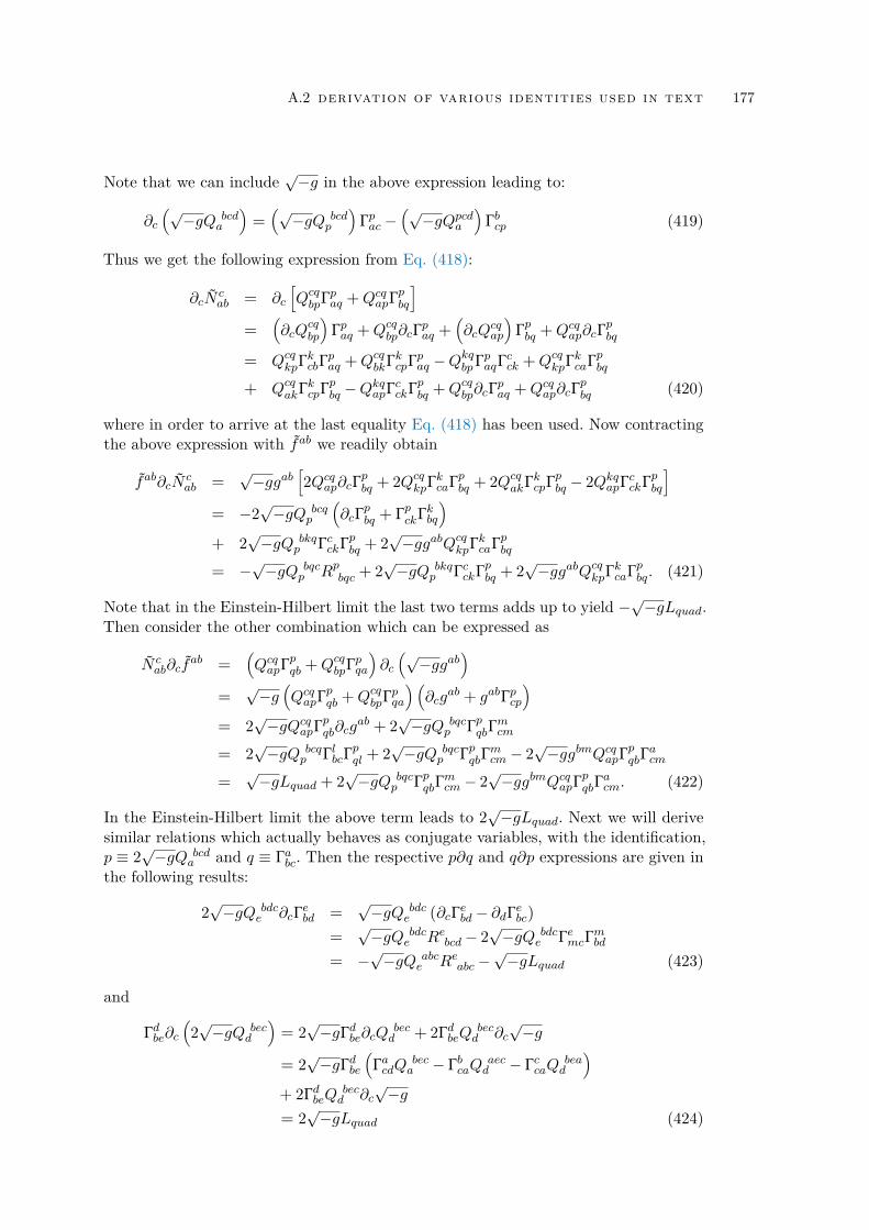
A.2 derivation of various identities used in text 177

Note that we can include √−g in the above expression leading to:

∂c(√−gQ bcd

a

)=(√−gQ bcd

p

)Γpac −

(√−gQpcda

)Γbcp (419)

Thus we get the following expression from Eq. (418):

∂cNcab = ∂c

[QcqbpΓpaq +QcqapΓpbq

]=

(∂cQ

cqbp

)Γpaq +Qcqbp∂cΓ

paq +

(∂cQ

cqap

)Γpbq +Qcqap∂cΓ

pbq

= QcqkpΓkcbΓpaq +QcqbkΓkcpΓpaq −Q

kqbpΓpaqΓ

cck +QcqkpΓkcaΓpbq

+ QcqakΓkcpΓpbq −QkqapΓcckΓpbq +Qcqbp∂cΓ

paq +Qcqap∂cΓ

pbq (420)

where in order to arrive at the last equality Eq. (418) has been used. Now contractingthe above expression with fab we readily obtain

fab∂cNcab =

√−ggab

[2Qcqap∂cΓ

pbq + 2QcqkpΓkcaΓpbq + 2QcqakΓkcpΓpbq − 2QkqapΓcckΓpbq

]= −2

√−gQ bcq

p

(∂cΓ

pbq + ΓpckΓkbq

)+ 2

√−gQ bkq

p ΓcckΓpbq + 2√−ggabQcqkpΓkcaΓpbq

= −√−gQ bqc

p Rpbqc + 2√−gQ bkq

p ΓcckΓpbq + 2√−ggabQcqkpΓkcaΓpbq. (421)

Note that in the Einstein-Hilbert limit the last two terms adds up to yield −√−gLquad.Then consider the other combination which can be expressed as

N cab∂cf

ab =(QcqapΓpqb +QcqbpΓpqa

)∂c(√−ggab

)=√−g

(QcqapΓpqb +QcqbpΓpqa

) (∂cg

ab + gabΓpcp)

= 2√−gQcqapΓpqb∂cg

ab + 2√−gQ bqc

p ΓpqbΓmcm

= 2√−gQ bcq

p ΓlbcΓpql + 2

√−gQ bqc

p ΓpqbΓmcm − 2

√−ggbmQcqapΓpqbΓ

acm

=√−gLquad + 2

√−gQ bqc

p ΓpqbΓmcm − 2

√−ggbmQcqapΓpqbΓ

acm. (422)

In the Einstein-Hilbert limit the above term leads to 2√−gLquad. Next we will derivesimilar relations which actually behaves as conjugate variables, with the identification,p ≡ 2√−gQ bcd

a and q ≡ Γabc. Then the respective p∂q and q∂p expressions are given inthe following results:

2√−gQ bdc

e ∂cΓebd =√−gQ bdc

e (∂cΓebd − ∂dΓebc)=√−gQ bdc

e Rebcd − 2√−gQ bdc

e ΓemcΓmbd

= −√−gQ abc

e Reabc −√−gLquad (423)

and

Γdbe∂c(2√−gQ bec

d

)= 2√−gΓdbe∂cQ

becd + 2ΓdbeQ

becd ∂c

√−g

= 2√−gΓdbe

(ΓacdQ

beca − ΓbcaQ

aecd − ΓccaQ

bead

)+ 2ΓdbeQ

becd ∂c

√−g

= 2√−gLquad (424)

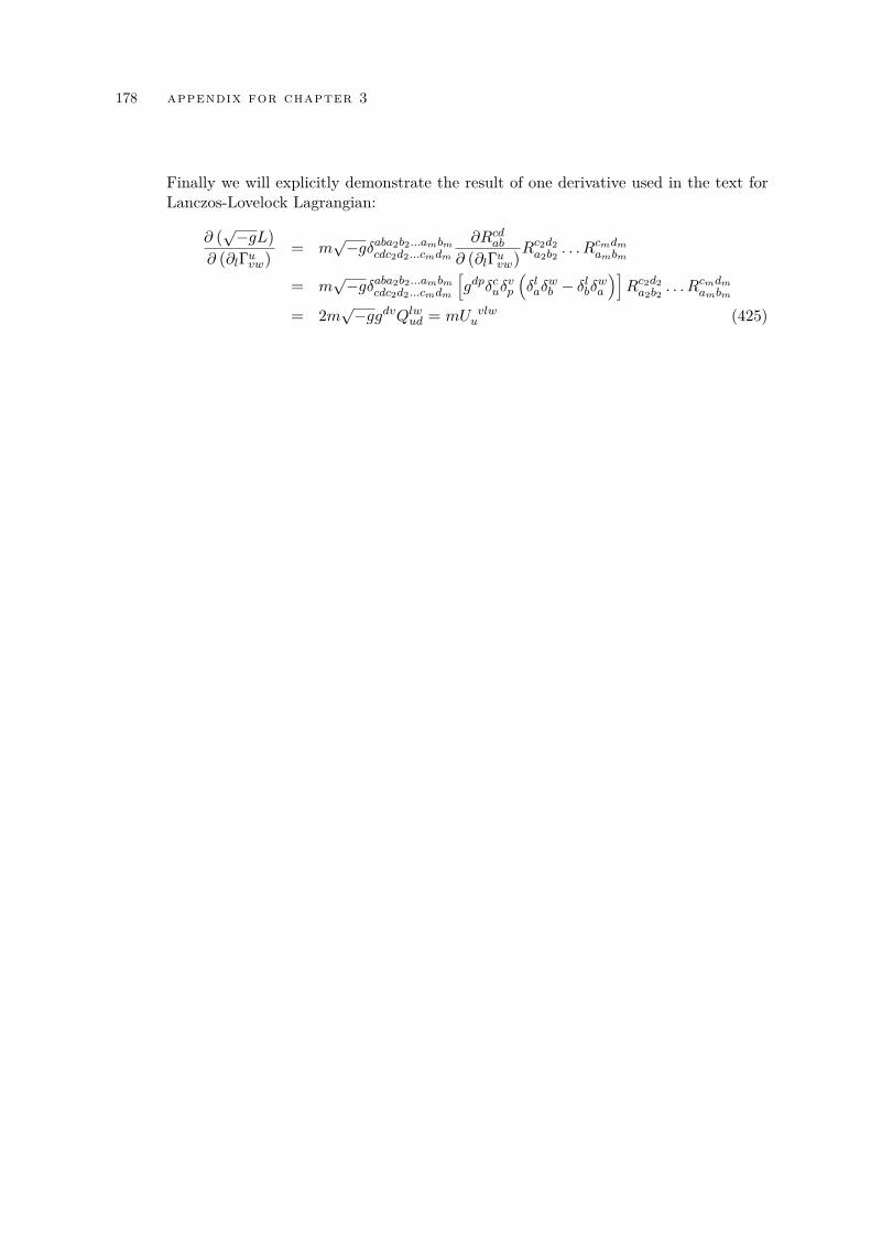
178 appendix for chapter 3

Finally we will explicitly demonstrate the result of one derivative used in the text forLanczos-Lovelock Lagrangian:

∂ (√−gL)

∂ (∂lΓuvw)= m

√−gδaba2b2...ambm

cdc2d2...cmdm

∂Rcdab∂ (∂lΓuvw)

Rc2d2a2b2

. . . Rcmdmambm

= m√−gδaba2b2...ambm

cdc2d2...cmdm

[gdpδcuδ

vp

(δlaδ

wb − δlbδwa

)]Rc2d2a2b2

. . . Rcmdmambm

= 2m√−ggdvQlwud = mU vlw

u (425)

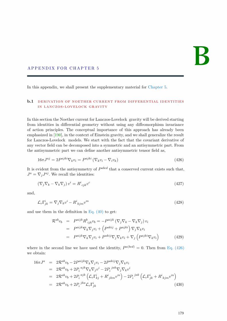
BAPPENDIX FOR CHAPTER 5

In this appendix, we shall present the supplementary material for Chapter 5.

b.1 derivation of noether current from differential identitiesin lanczos-lovelock gravity

In this section the Noether current for Lanczos-Lovelock gravity will be derived startingfrom identities in differential geometry without using any diffeomorphism invarianceof action principles. The conceptual importance of this approach has already beenemphasized in [190], in the context of Einstein gravity, and we shall generalize the resultfor Lanczos-Lovelock models. We start with the fact that the covariant derivative ofany vector field can be decomposed into a symmetric and an antisymmetric part. Fromthe antisymmetric part we can define another antisymmetric tensor field as,

16πJaj = 2P ajki∇kvi = P ajki (∇kvi −∇ivk) (426)

It is evident from the antisymmetry of P abcd that a conserved current exists such that,Ja = ∇jJaj . We recall the identities:

(∇j∇k −∇k∇j) vi = Ricjkvc (427)

and,

LvΓijk = ∇j∇kvi −Rikjmvm (428)

and use them in the definition in Eq. (40) to get:

Rabvb = P aijkRbijkvb = −P aijk (∇j∇k −∇k∇j) vi= P aijk∇k∇jvi +

(P akij + P ajki

)∇j∇kvi

= P aijk∇k∇jvi + P akij∇j∇kvi +∇j(P ajki∇kvi

)(429)

where in the second line we have used the identity, P a(bcd) = 0. Then from Eq. (426)we obtain:

16πJa = 2Rabvb − 2P aijk∇k∇jvi − 2P akij∇j∇kvi= 2Rabvb + 2P ajk

i ∇k∇jvi − 2P jaki ∇j∇kvi

= 2Rabvb + 2P ajki

(LvΓikj +Rijkmv

m)− 2P jak

i

(LvΓijk +Rikjmv

m)

= 2Rabvb + 2P jkai LvΓijk (430)

179

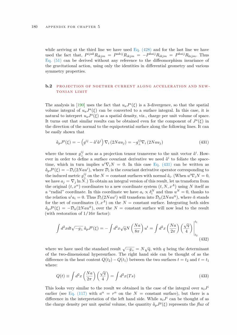
180 appendix for chapter 5

while arriving at the third line we have used Eq. (428) and for the last line we haveused the fact that, P ijakRikjm = P akijRikjm = −P kaijRikjm = P kaijRkijm. ThusEq. (51) can be derived without any reference to the diffeomorphism invariance ofthe gravitational action, using only the identities in differential geometry and varioussymmetry properties.

b.2 projection of noether current along acceleration and new-tonian limit

The analysis in [190] uses the fact that uaJa(ξ) is a 3-divergence, so that the spatialvolume integral of uaJa(ξ) can be converted to a surface integral. In this case, it isnatural to interpret uaJa(ξ) as a spatial density, viz., charge per unit volume of space.It turns out that similar results can be obtained even for the component of Ja(ξ) inthe direction of the normal to the equipotential surface along the following lines. It canbe easily shown that

apJp(ξ) = −

(gij − aiaj

)∇i (2Nauj) = −gij⊥∇i (2Nauj) (431)

where the tensor gij⊥ acts as a projection tensor transverse to the unit vector ai. How-ever in order to define a surface covariant derivative we need ai to foliate the space-time, which in turn implies ui∇iN = 0. In this case Eq. (431) can be written asapJ

p(ξ) = −Di(2Naui), where Di is the covariant derivative operator corresponding tothe induced metric gij⊥ on the N = constant surfaces with normal ai. (When ui∇iN = 0,we have aj = ∇j lnN .) To obtain an integral version of this result, let us transform fromthe original (t,xα) coordinates to a new coordinate system (t,N ,xA) using N itself asa “radial” coordinate. In this coordinate we have ai ∝ δNi and thus uN = 0, thanks tothe relation uiai = 0. Thus Di(2Naui) will transform into Dα(2Nauα), where α standsfor the set of coordinates (t,xA) on the N = constant surface. Integrating both sidesapJ

p(ξ) = −Dα(2Nauα), over the N = constant surface will now lead to the result(with restoration of 1/16π factor):

∫d2xdt

√−g⊥ apJp(ξ) = −

∫d2x√qN

(Na

8π

)ut =

∫d2x

(Na

2π

)(√q

4

) ∣∣∣∣∣∣t1

t2

(432)

where we have used the standard result √−g⊥ = N√q, with q being the determinant

of the two-dimensional hypersurface. The right hand side can be thought of as thedifference in the heat content Q(t2)−Q(t1) between the two surfaces t = t2 and t = t1where:

Q(t) ≡∫d2x

(Na

2π

)(√q

4

)=∫d2x(Ts) (433)

This looks very similar to the result we obtained in the case of the integral over uiJ iearlier (see Eq. (117) with aα = rα on the N = constant surface), but there is adifference in the interpretation of the left hand side. While uiJ i can be thought of asthe charge density per unit spatial volume, the quantity apJp(ξ) represents the flux of

B.3 identities regarding noether current in lanczos-lovelock action 181

Noether current through a time-like surface; therefore, apJp(ξ) should be thought of asa current per unit area per unit time. We will see later that the flux of Noether currentthrough null surfaces leads to a very similar result.

We conclude this section with a discussion of the Newtonian limit of general relativityusing the Noether current which has some amusing features. The Newtonian limit isobtained by setting N2 = 1 + 2φ, g0α = 0 and gαβ = δαβ, where φ is the Newtonianpotential [232]. Then the acceleration of the fundamental observers turn out to beaα = ∂αφ. Since the spatial section of the spacetime is flat, the extrinsic curvatureidentically vanishes and so does the Lie variation term. Also 2Tabuaub = ρKomar = ρ,which immediately leads to (with G inserted, see Eq. (118)):

∇2φ = 4πGρ (434)

the correct Newtonian limit. The same can also be obtained using the four velocityua. The Noether charge associated with ua turns out to have the following expression[190]

Dαaα = 16πuaJa(u) = 16πTabuaub + uag

bc£uNabc (435)

In the Newtonian limit the following results hold 2Tabuaub = ρ and uagbc£uN

abc =

−Dαaα (which follows from the Newtonian limit of the result uagbc£ξN

abc = NDαa

α +2aαDαN −Nuagij£uN

aij and the fact that in spacetime with flat spatial section the

term uagbc£ξN

abc identically vanishes). This immediately leads to Eq. (434).

We also see that the Noether charge is positive as long as ρ > 0 in the Newtonianlimit. In fact, the Noether charge contained inside any equipotential surface is alwaysa positive definite quantity as long as rα and aα point in the same direction (whichhappens when Tabuaub > 0). To prove this we can integrate the Noether charge over asmall region on a t = constant hypersurface to obtain,∫

t=constantd3x√huaJ

a(u) =1

8π

∫N ,t=constant

d2x√q2Naαrα

=∫N ,t=constant

d2x

(Na

2π

)(√q

4

)(436)

Since ρ is positive definite in this case the fundamental observers are acceleratingoutwards and thus rαaα = a. The temperature as measured by these fundamentalobservers is a positive definite quantity and so is the entropy density and hence thepositivity of Noether charge follows.

b.3 identities regarding noether current in lanczos-lovelockaction

The Noether potential Jab is antisymmetric in (a, b) and from its expression given byEq. (50) it is evident that Jab(q) would identically vanish for qa = ∇aφ. We will usethe above fact in order to obtain a relation between the Noether current for two vectorfields qa and va connected by va = f(x)qa. This result, in the case of general relativity

182 appendix for chapter 5

is detailed in [190]. While in the case of Lanczos-Lovelock gravity the Noether currentfor a vector field va = f(x)qa can be decomposed as:

16πJab(v) = 2P abcd∇c (fqd)= 2P abcdqd∇cf + 2fP abcd∇cqd (437)

Then the corresponding Noether current has the following expression:

16πJa(v) = 2P abcd∇b (qd∇cf) + 2P abcd∇b (f∇cqd)= 2P abcdqd∇b∇cf + 2P abcd∇cf∇bqd+ 2P abcd∇bf∇cqd + 2fP abcd∇b∇cqd (438)

From the above equation we readily arrive at:

16π Ja(v)− fJa(q) = 2P abcdqd∇b∇cf + 2P abcd∇cf∇bqd + 2P abcd∇bf∇cqd= P abcd∇bAcd + 16πJab(q)∇bf (439)

where we have defined the antisymmetric tensor Acd as Acd = qd∇cf − qc∇df . Nowconsider the following result: qa∇bAcd = ∇b (qaAcd)−Acd∇bqa which leads to:

P abcdqa∇bAcd = ∇b(P abcdqaAcd

)− 2P abcdqd∇cf∇bqa

= ∇b(P abcdqaAcd

)− 16πqaJab (q)∇bf (440)

Then Eq. (439) can be rewritten in the following manner:

16π qaJa(fq)− fqaJa(q) = 16πJab(q)∇bfqa +∇b(P abcdqaAcd

)− 16πqaJab(q)∇bf

= ∇b(2P abcdqaqd∇cf

)(441)

It can be easily verified that in the Einstein-Hilbert limit P abcd = Qabcd = (1/2)(gacgbd − gadgbc

),

under which the above equation reduces to the respective one in general relativity.

Applying the above equation to ua = −N∇at with qa = ∇at = −ua/N and f = −Nwe arrive at:

16πuaJa (u) = 2N∇b(P abcduaud

∇cNN2

)(442)

In order to proceed we define a new vector field such that:

χa = −2P abcdubud∇cNN

= −2P abcdubud(ac −

1Nucu

j∇jN)

= −2P abcdubacud (443)

Note that in the Einstein-Hilbert limit this vector reduces to the acceleration fourvector as follows:

χa = −2P abcdubacud = −(gacgbd − gadgbc

)ubacud = −ububaa+ ubabu

a = aa (444)

B.3 identities regarding noether current in lanczos-lovelock action 183

Also just as in the case of acceleration for the vector χa as well we have:

uaχa = −2aP abβduaubrβud = 0 (445)

where antisymmetry of P abcd in the first two components has been used. We can alsohave the following relation for the vector field χa:

Nabχb = χb∇bN + χbubu

j∇jN = χb∇bN (446)

where we have used the relation uaχa = 0 from Eq. (445). Thus Eq. (442) can be

written in terms of the newly defined vector field χa in the following way:

16πuaJa (u) = N∇b

(χb

N

)

= ∇bχb −∇bNN

χb

= Dαχα (447)

The last relation follows from the fact that:

Dαχα = Dbχ

b = ∇bχb − abχb = ∇bχb −∇bNN

χb (448)

Then it is straightforward to get the Noether current for ξa by using qa = ua andf = N in Eq. (441) with Eq. (447) as:

16πuaJa (ξ) = 16πNuaJa(u) +∇b(Nχb

)= NDαχ

α +∇b(Nχb

)= Dα (2Nχα) (449)

Here also we have used the following identity:

Dα (Nχα) =

(gij + uiuj

)∇i (Nχj)

= ∇i(Nχi

)+ uiuj∇i (Nχj)

= N∇iχi +Nχiai −Nχj(ui∇iuj

)= N∇iχi (450)

Thus we have derived the desired relation for the Noether current of the vector field ξaand it turns out to have identical structure as that of Einstein-Hilbert action with χaplaying the role of four acceleration.

CAPPENDIX FOR CHAPTER 6

In this appendix, we shall present the supplementary material for Chapter 6.

c.1 detailed expressions regarding first law

Let us start with evaluating the following expression in GNC coordinates introducedin the main text, which leads to

12

(Euu +Err

)= Euu = Err

= −12

116π

12m δ

ra1b1...ambmrc1d1...cmdm

Rc1d1a1b1

. . . Rcmdmambm

= − m

16π1

2m−1 δruPA1B1...Am−1Bm−1ruQC1D1...Cm−1Dm−1

RuQuPRC1D1A1B1

. . . RCm−1Dm−1Am−1Bm−1

− m(m− 1)16π

12m−1 δ

ruPA1B1...Am−1Bm−1ruQC1D1...Cm−1Dm−1

RQC1uP RuD1

A1B1. . . R

Cm−1Dm−1Am−1Bm−1

− 116π

12m+1 δ

rA1B1...AmBmrC1D1...CmDm

RC1D1A1B1

. . . RCmDmAmBm(451)

Then we obtain:

T rr = 2Err = −m

8π1

2m−1 δPA1B1...Am−1Bm−1QC1D1...Cm−1Dm−1

RuQuPRC1D1A1B1

. . . RCm−1Dm−1Am−1Bm−1

− m(m− 1)8π

12m−1 δ

PA1B1...Am−1Bm−1QC1D1...Cm−1Dm−1

RQC1uP RuD1

A1B1. . . R

Cm−1Dm−1Am−1Bm−1

− 116π

12m δ

A1B1...AmBmC1D1...CmDm

RC1D1A1B1

. . . RCmDmAmBm(452)

Now we have the following expression for components of Riemann tensor as:

RuQuP = −12q

QE∂u∂rqPE −12q

QE∂PβE −12αq

QE∂rqPE −14β

QβP

+14(qQE∂rqPF

) (qFL∂uqEL

)+

12q

QEβAΓAEP (453a)

RAMCD = RAMCD −14q

AEqMB∂uqCE∂rqBD + ∂rqCE∂uqBD − (C ↔ D)

(453b)

RuNCD = −12q

MN∂r∂CqMD −14βCq

MN∂rqMD −12(qMN∂rqCE

)ΓEMD − (C ↔ D)

(453c)

RABuC = qBD[∂uΓADC −

12q

AE∂C∂uqDE −12∂Cq

AE∂uqDE +14β

A∂uqCD

+12q

AF∂uqEF ΓECD −14βDq

AE∂uqEC −12q

EF∂uqFDΓACE

](453d)

185

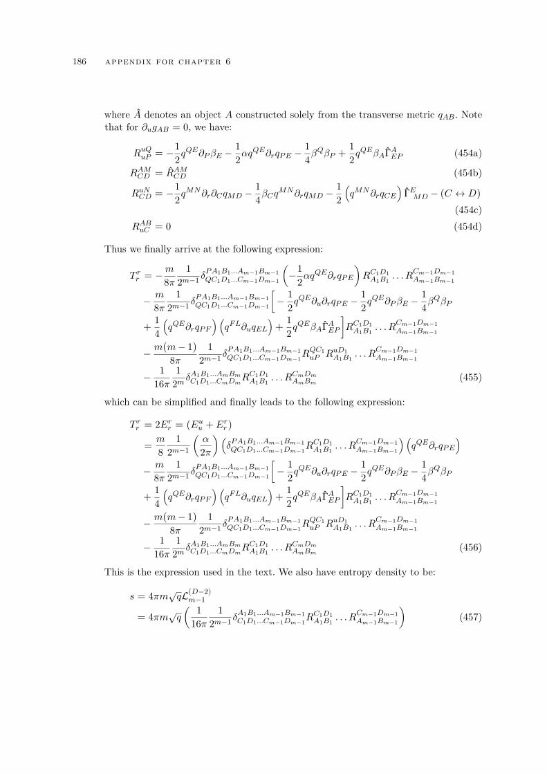
186 appendix for chapter 6

where A denotes an object A constructed solely from the transverse metric qAB. Notethat for ∂ugAB = 0, we have:

RuQuP = −12q

QE∂PβE −12αq

QE∂rqPE −14β

QβP +12q

QEβAΓAEP (454a)

RAMCD = RAMCD (454b)

RuNCD = −12q

MN∂r∂CqMD −14βCq

MN∂rqMD −12(qMN∂rqCE

)ΓEMD − (C ↔ D)

(454c)RABuC = 0 (454d)

Thus we finally arrive at the following expression:

T rr = −m8π1

2m−1 δPA1B1...Am−1Bm−1QC1D1...Cm−1Dm−1

(−1

2αqQE∂rqPE

)RC1D1A1B1

. . . RCm−1Dm−1Am−1Bm−1

− m

8π1

2m−1 δPA1B1...Am−1Bm−1QC1D1...Cm−1Dm−1

[− 1

2qQE∂u∂rqPE −

12q

QE∂PβE −14β

QβP

+14(qQE∂rqPF

) (qFL∂uqEL

)+

12q

QEβAΓAEP

]RC1D1A1B1

. . . RCm−1Dm−1Am−1Bm−1

− m(m− 1)8π

12m−1 δ

PA1B1...Am−1Bm−1QC1D1...Cm−1Dm−1

RQC1uP RuD1

A1B1. . . R

Cm−1Dm−1Am−1Bm−1

− 116π

12m δ

A1B1...AmBmC1D1...CmDm

RC1D1A1B1

. . . RCmDmAmBm(455)

which can be simplified and finally leads to the following expression:

T rr = 2Err = (Euu +Err )

=m

81

2m−1

(α

2π

)(δPA1B1...Am−1Bm−1QC1D1...Cm−1Dm−1

RC1D1A1B1

. . . RCm−1Dm−1Am−1Bm−1

) (qQE∂rqPE

)− m

8π1

2m−1 δPA1B1...Am−1Bm−1QC1D1...Cm−1Dm−1

[− 1

2qQE∂u∂rqPE −

12q

QE∂PβE −14β

QβP

+14(qQE∂rqPF

) (qFL∂uqEL

)+

12q

QEβAΓAEP

]RC1D1A1B1

. . . RCm−1Dm−1Am−1Bm−1

− m(m− 1)8π

12m−1 δ

PA1B1...Am−1Bm−1QC1D1...Cm−1Dm−1

RQC1uP RuD1

A1B1. . . R

Cm−1Dm−1Am−1Bm−1

− 116π

12m δ

A1B1...AmBmC1D1...CmDm

RC1D1A1B1

. . . RCmDmAmBm(456)

This is the expression used in the text. We also have entropy density to be:

s = 4πm√qL(D−2)m−1

= 4πm√q( 1

16π1

2m−1 δA1B1...Am−1Bm−1C1D1...Cm−1Dm−1

RC1D1A1B1

. . . RCm−1Dm−1Am−1Bm−1

)(457)

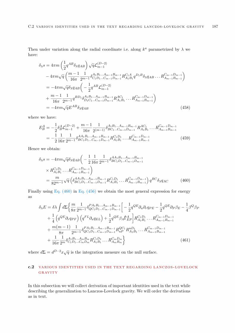
C.2 various identities used in the text regarding lanczos-lovelock gravity 187

Then under variation along the radial coordinate i.e. along ka parametrized by λ wehave:

δλs = 4πm(1

2qABδλqAB

)√qL(D−2)

m−1

− 4πm√q(m− 116π

12m−1 δ

A1B1...Am−1Bm−1C1D1...Cm−1Dm−1

RC1AA1B1

qD1BδλqAB . . . RCm−1Dm−1Am−1Bm−1

)= −4πm√qδλqAB

(− 1

2qABL(D−2)

m−1

+m− 116π

12m−1 q

BD1δA1B1...Am−1Bm−1D1C1...Cm−1Dm−1

RAC1A1B1

. . . RCm−1Dm−1Am−1Bm−1

)= −4πm√qEABδλqAB (458)

where we have:

EAB = −12δ

ABL

(D−2)m−1 +

m− 116π

12(m−1) δ

A1B1...Am−1Bm−1BC1...Cm−1Dm−1

RAC1A1B1

. . . RCm−1Dm−1Am−1Bm−1

= −12

116π

12m−1 δ

AA1B1...Am−1Bm−1BC1D1...Cm−1Dm−1

RC1D1A1B1

. . . RCm−1Dm−1Am−1Bm−1

(459)

Hence we obtain:

δλs = −4πm√qδλqAB(− 1

21

16π1

2m−1 δAA1B1...Am−1Bm−1BC1D1...Cm−1Dm−1

×RC1D1A1B1

. . . RCm−1Dm−1Am−1Bm−1

)=

m

82m−1√q(δAA1B1...Am−1Bm−1BC1D1...Cm−1Dm−1

RC1D1A1B1

. . . RCm−1Dm−1Am−1Bm−1

)qBCδλqAC (460)

Finally using Eq. (460) in Eq. (456) we obtain the most general expression for energyas

δλE = δλ

∫dΣm

8π1

2m−1 δPA1B1...Am−1Bm−1QC1D1...Cm−1Dm−1

[− 1

2qQE∂u∂rqPE −

12q

QE∂PβE −14β

QβP

+14(qQE∂rqPF

) (qFL∂uqEL

)+

12q

QEβAΓAEP

]RC1D1A1B1

. . . RCm−1Dm−1Am−1Bm−1

+m(m− 1)

8π1

2m−1 δPA1B1...Am−1Bm−1QC1D1...Cm−1Dm−1

RQC1uP RuD1

A1B1. . . R

Cm−1Dm−1Am−1Bm−1

+1

16π1

2m δA1B1...AmBmC1D1...CmDm

RC1D1A1B1

. . . RCmDmAmBm

(461)

where dΣ = dD−2x√q is the integration measure on the null surface.

c.2 various identities used in the text regarding lanczos-lovelockgravity

In this subsection we will collect derivation of important identities used in the text whiledescribing the generalization to Lanczos-Lovelock gravity. We will order the derivationsas in text.

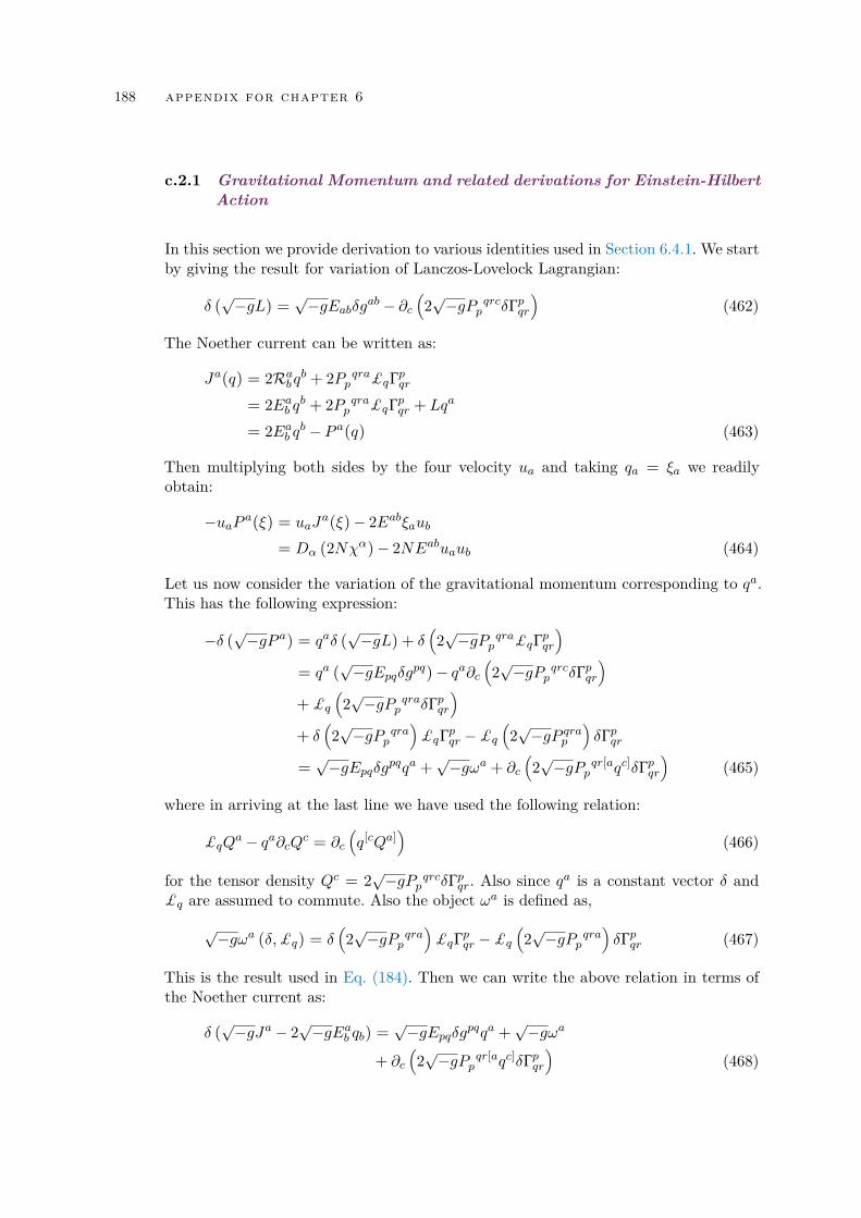
188 appendix for chapter 6

c.2.1 Gravitational Momentum and related derivations for Einstein-HilbertAction

In this section we provide derivation to various identities used in Section 6.4.1. We startby giving the result for variation of Lanczos-Lovelock Lagrangian:

δ (√−gL) =

√−gEabδgab − ∂c

(2√−gP qrc

p δΓpqr)

(462)

The Noether current can be written as:

Ja(q) = 2Rabqb + 2P qrap £qΓpqr

= 2Eab qb + 2P qrap £qΓpqr + Lqa

= 2Eab qb − P a(q) (463)

Then multiplying both sides by the four velocity ua and taking qa = ξa we readilyobtain:

−uaP a(ξ) = uaJa(ξ)− 2Eabξaub

= Dα (2Nχα)− 2NEabuaub (464)

Let us now consider the variation of the gravitational momentum corresponding to qa.This has the following expression:

−δ (√−gP a) = qaδ (

√−gL) + δ

(2√−gP qra

p £qΓpqr)

= qa (√−gEpqδgpq)− qa∂c

(2√−gP qrc

p δΓpqr)

+ £q

(2√−gP qra

p δΓpqr)

+ δ(2√−gP qra

p

)£qΓpqr −£q

(2√−gP qrap

)δΓpqr

=√−gEpqδgpqqa +

√−gωa + ∂c

(2√−gP qr[a

p qc]δΓpqr)

(465)

where in arriving at the last line we have used the following relation:

£qQa − qa∂cQc = ∂c

(q[cQa]

)(466)

for the tensor density Qc = 2√−gP qrcp δΓpqr. Also since qa is a constant vector δ and

£q are assumed to commute. Also the object ωa is defined as,√−gωa (δ, £q) = δ

(2√−gP qra

p

)£qΓpqr −£q

(2√−gP qra

p

)δΓpqr (467)

This is the result used in Eq. (184). Then we can write the above relation in terms ofthe Noether current as:

δ (√−gJa − 2

√−gEab qb) =

√−gEpqδgpqqa +

√−gωa

+ ∂c(2√−gP qr[a

p qc]δΓpqr)

(468)

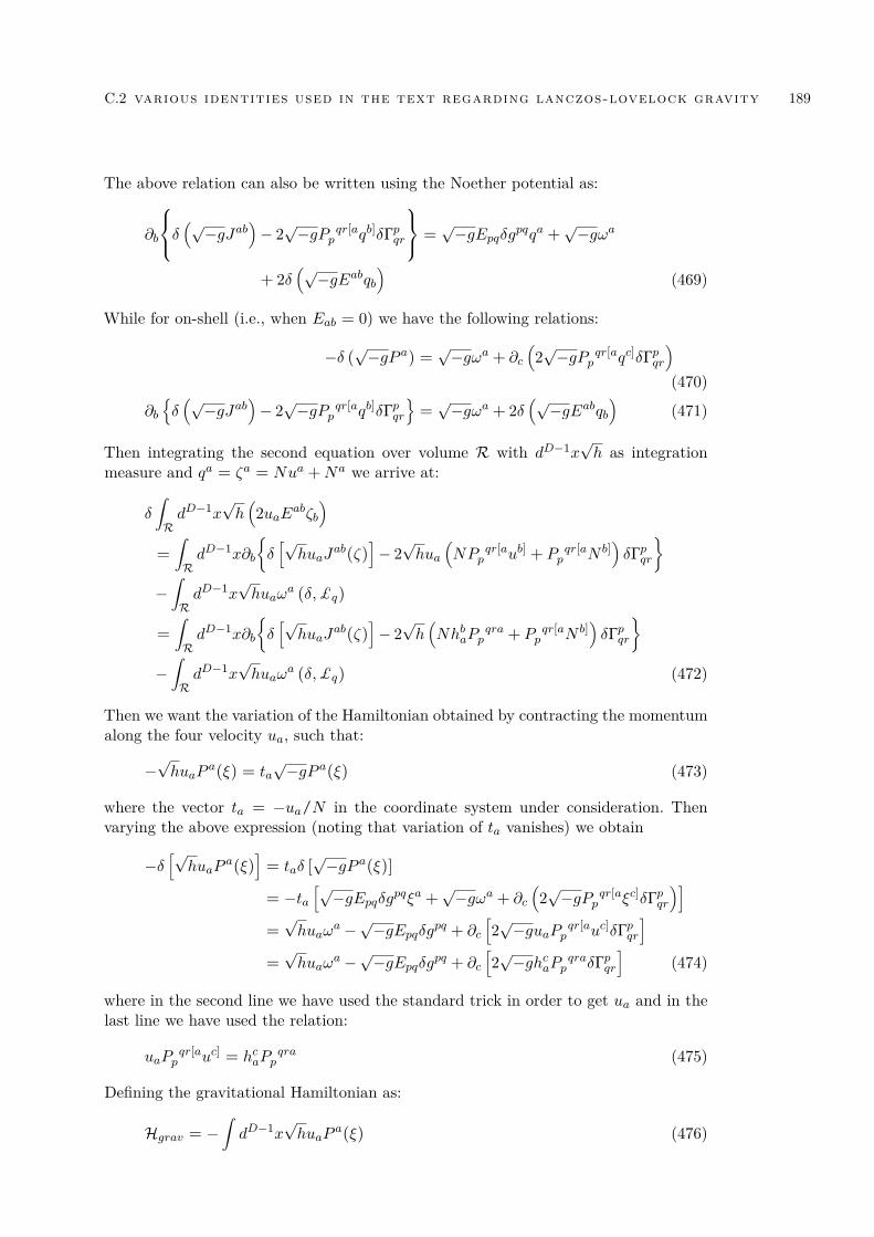
C.2 various identities used in the text regarding lanczos-lovelock gravity 189

The above relation can also be written using the Noether potential as:

∂b

δ (√−gJab)− 2√−gP qr[a

p qb]δΓpqr

=√−gEpqδgpqqa +

√−gωa

+ 2δ(√−gEabqb

)(469)

While for on-shell (i.e., when Eab = 0) we have the following relations:

−δ (√−gP a) =

√−gωa + ∂c

(2√−gP qr[a

p qc]δΓpqr)(470)

∂bδ(√−gJab

)− 2√−gP qr[a

p qb]δΓpqr=√−gωa + 2δ

(√−gEabqb

)(471)

Then integrating the second equation over volume R with dD−1x√h as integration

measure and qa = ζa = Nua +Na we arrive at:

δ

∫RdD−1x

√h(2uaEabζb

)=∫RdD−1x∂b

δ[√huaJ

ab(ζ)]− 2√hua

(NP qr[a

p ub] + P qr[ap N b]

)δΓpqr

−∫RdD−1x

√huaω

a (δ, £q)

=∫RdD−1x∂b

δ[√huaJ

ab(ζ)]− 2√h(NhbaP

qrap + P qr[a

p N b])δΓpqr

−∫RdD−1x

√huaω

a (δ, £q) (472)

Then we want the variation of the Hamiltonian obtained by contracting the momentumalong the four velocity ua, such that:

−√huaP

a(ξ) = ta√−gP a(ξ) (473)

where the vector ta = −ua/N in the coordinate system under consideration. Thenvarying the above expression (noting that variation of ta vanishes) we obtain

−δ[√huaP

a(ξ)]= taδ [

√−gP a(ξ)]

= −ta[√−gEpqδgpqξa +

√−gωa + ∂c

(2√−gP qr[a

p ξc]δΓpqr)]

=√huaω

a −√−gEpqδgpq + ∂c

[2√−guaP qr[a

p uc]δΓpqr]

=√huaω

a −√−gEpqδgpq + ∂c

[2√−ghcaP qra

p δΓpqr]

(474)

where in the second line we have used the standard trick in order to get ua and in thelast line we have used the relation:

uaPqr[ap uc] = hcaP

qrap (475)

Defining the gravitational Hamiltonian as:

Hgrav = −∫dD−1x

√huaP

a(ξ) (476)

190 appendix for chapter 6

its variation can be obtained readily from Eq. (474) as:

δHgrav =∫dD−1x

√huaω

a−∫dD−1x

√−gEpqδgpq+

∫dD−2x 2rc

√qP qrc

p δΓpqr (477)

where in order to obtain the last term we have used the result that rchca = ra and√−g = N

√h. The above results are true for arbitrary variations. Applying it to Lie

variation along ξa we arrive at the following form for Eq. (474) as:

−£ξ

[√huaP

a(ξ)]= 2√−gEpq∇pξq + ∂c

[2√−ghcaP qra

p £ξΓpqr]

(478)

In arriving at the above result we have used the relations: £ξgab = −(∇aξb +∇bξa)

and ωa(£ξ, £ξ) = 0. Now using Bianchi identity ∇aEab = 0 we arrive at:

−£ξ

[√huaP

a(ξ)]= ∂c

[2√−g

(Ecdξd + hcaP

qrap £ξΓpqr

)](479)

This is the relation used to arrive at the results in the main text.

c.2.2 Characterizing Null Surfaces

Let us now try to generalize the result for null surfaces to Lovelock gravity with thenull vector `a such that `2 = 0 everywhere. For that purpose, we start with the combi-nation:

Rab`a`b = RapqrPpqrb `a`b

= P bpqr`b (Rapqr`a)

= −P bpqr`b (∇q∇r`p −∇r∇q`p)= −2P bpqr`b∇q∇r`p= ∇q

(−2P bpqr`b∇r`p

)−S (480)

where we have defined, the entropy density as:

S = −2P bpqr∇q`b∇r`p (481)

The Einstein-Hilbert limit can be obtained easily leading to:

16πS = −(gbqgpr − gbrgpq

)∇q`b∇r`p

= ∇a`b∇b`a −(∇i`i

)2(482)

as well as,

32πP bpqr`b∇r`p =(gbqgpr − gbrgpq

)`b∇r`p

= `q∇r`r − `r∇r`q

= Θ`q (483)

However in Lanczos-Lovelock gravity, the combination, 2P bpqr`b∇r`p cannot be writtenas, φ`q, for arbitrary φ, since 2P bpqr`q`b∇r`p 6= 0. Next let us consider the object,

C.2 various identities used in the text regarding lanczos-lovelock gravity 191

`aJa (`), for which we define, `a = A∇aB. Then in Lanczos-Lovelock gravity, we arrive

at:1A`aJ

a (`) = ∇b[2P abcd`a`d∇cA

1A2

]=

1A∇b[2P abcd`a`d∇c lnA

]− 1A

[2P abcd`a`d∇c lnA∇b lnA

](484)

Let us now expand ∇c lnA in canonical null basis, such that we obtain,

∇c lnA = −κkc +A`c +BAeAc (485)

Note that we obtain, `c∇c lnA = κ. In a similar fashion, we can expand, 2P abcd`a`d∇c lnAin the following manner,

2P abcd`a`d∇c lnA = P`b +Qkb +RAebA (486)

It is evident that Q = −2P abcd`a`d`b∇c lnA = 0, due to antisymmetry of P abcd in thefirst two indices. Then it turns out that,

P = −2P abcd`akb`d∇c lnA ≡ K (487)

It is obvious from the Einstein-Hilbert limit, that

16πK = −(gacgbd − gadgbc

)`akb`d∇c lnA

= −(gacgbd − gadgbc

)`akb`d

(−κkc +BAe

Ac

)= κ (488)

Also in the expansion for, ∇c lnA, we obtain, BA is completely arbitrary. Then wecan use BA such that the following relation: BQP abcd`a`deAb eQc = κP abcd`akc`de

Ab is

satisfied, such that, RA vanishes. Thus we obtain,

2P abcd`a`d∇c lnA = K`b (489)

Again, we get,

2P abcd`a`d∇c lnA∇b lnA = K`b∇b lnA = κK (490)

Thus, finally we arrive at the following result:

`aJa (`) = ∇a (K`a)− κK (491)

Again by considering derivative on the null surface, we obtain,

Da (K`a) =(gab + `akb + `bka

)∇a (K`b)

= ∇a (K`a) + kb`a∇a (K`b)= ∇a (K`a)− κK− `a∇aK (492)

Thus the Noether current contraction can also be written as:

`aJa (`) = Da (K`a) +

dKdλ

(493)

DAPPENDIX FOR CHAPTER 7

In this appendix, we shall present the supplementary material for Chapter 7.

d.1 general analysis regarding null surfaces

We will start with a null vector `a = A∇aB, which satisfies the condition `2 = 0only over a single surface, which is the null surface under our consideration. Then weobtain

`a∇a`b = κ`b (494)

where we have the following expression for κ

κ = `a∂a lnA+ κ; κ = −12k

a∂a`2 (495)

The last relation defining κ can also be written as ∇a`2 = 2κ`a. The derivation of theresult goes as follows, let us expand ∇b`2 in canonical null basis, i.e., ∇a`2 = C`a +Dka + EAe

Aa . Then both EA = eaA∇a`2 and D = −`a∇a`2 vanishes, since variation

of `2 along the null surface vanishes. This shows that the only non-zero component of∇a`2 is along `a. Then it turns out that [202]

∇i`i = Θ + κ+ κ (496)

where, Θ = qmaqmb∇a`b. Note that the term κ enters the picture as `2 = 0 only on thenull surface. With this setup let us now find out Rab`a`b in detail, which leads to,

Rab`a`b = `j

(∇i∇j`i −∇j∇i`i

)= ∇i

(`j∇j`i

)−∇j

(`j∇i`i

)−∇i`j∇j`i +

(∇i`i

)2

= ∇i(`j∇j`i − `i∇j`j

)−(∇i`j∇j`i −

(∇i`i

)2)

(497)

However in general, `j∇j`i = κ`i is not true, it only holds on the null surface (when `2 =0 everywhere this relation is also true everywhere). Since we were doing the calculationfor the most general case, `2 6= 0 in the above expression we cannot substitute `j∇j`i =κ`i, since it appears inside the derivative. Thus for the special case when `2 = 0everywhere, we will arrive at the following result

Rab`a`b = −∇i

(Θ`i

)−(∇i`j∇j`i −

(∇i`i

)2)

(498)

193

194 appendix for chapter 7

In order to simplify things quiet a bit we will compute the last term(∇i`j∇j`i −

(∇i`i

)2)which we designate by S. Then we start by calculating the following object on the nullsurface

Θab = qamqbn∇m`n

= (δam + `akm + ka`m)(δbn + `bkn + kb`n

)∇m`n

= ∇a`b + `akm∇m`b + κka`b + `bkn∇a`n + `a`bkmkn∇m`n

− κka`b + κ`akb − κ`akb + κkakb`2

= ∇a`b + `akm∇m`b + `bkn∇a`n + `a`bkmkn∇m`n (499)

In arriving at the third line we have used the following results: `a∇a`i = κ`i and`a∇b`a = κ`b. Then we can reverse the above equation leading to

∇a`b = Θab − `akm∇m`b − `bkn∇a`n − `a`bkmkn∇m`n (500)

From the above equation we can derive two very important identity:

(∇a`b)(∇a`b

)= ΘabΘab + `a`bk

m∇m`bkn∇a`n + `a`bkn∇a`nkm∇m`b

= ΘabΘab + 2 (κkm`m) (κ`nkn)= ΘabΘab + 2κκ (501)

In the same spirit we will arrive at

(∇a`b)(∇b`a

)= ΘabΘab + `a`bkn∇a`nkm∇b`m + `a`

bkm∇m`akn∇n`b= ΘabΘab + (κkm`m) (κk

n`n) + (κ`nkn) (κ`mk

m)

= ΘabΘab + κ2 + κ2 (502)

The extrinsic curvature for null surfaces, i.e., Θab can be given a very natural interpre-tation. This essentially follows from [202]. There the expression for Θab in terms of Lievariation of qab along the null generator `a was obtained as,

Θab =12q

ma q

nb £`qmn (503)

Now expanding out the Lie derivative term we obtain,

£`qmn = `i∂iqmn + qma∂n`a + qan∂m`

a (504)

Which on being substituted in Eq. (503) immediately leads to,

Θab =12q

ma q

nb `i∂iqmn +

12qaiq

nb ∂n`

i +12qbiq

ma ∂m`

i (505)

Now on the null surface qab = qAB as the only non-zero component. Hence the aboveequation can be written as,

Θab = ΘAB =12d

dλqAB +

12qAC∂B`

C +12qBC∂A`

C (506)

D.1 general analysis regarding null surfaces 195

On the null surface qab `b = 0, which in this coordinate system leads to `A = 0 on thenull surface. Since ∂A`2 represent derivatives on the null surface it also vanishes. If`2 = 0 everywhere, then also `A is identically zero everywhere. Hence we have

Θab =12d

dλqAB (507)

There is another way to get this result. If eaA are the basis vectors on the null surfaceand if `a, eaA forms coordinate basis vectors, then qAB = qabe

aAe

bB is a scalar under

4-dimensional coordinate transformation. This immediately leads to the previous ex-pression. For more discussions along identical lines see [202].

Now the expression for the quantity S can be obtained as

S = ∇i`j∇j`i −(∇i`i

)2

= ΘabΘab + κ2 + κ2 − (Θ + κ+ κ)2

=(

ΘabΘab −Θ2)− 2Θ (κ+ κ)− 2κκ (508)

Using the general expression for Rab`a`b we obtain the following form:

Rab`a`b = ∇i

(`j∇j`i − `i∇j`j

)−S

= ∇i(`j∇j`i − `i∇j`j

)−(

ΘabΘab −Θ2)+ 2Θ (κ+ κ) + 2κκ (509)

For the situation where, `2 = 0 everywhere we finally arrive at the following simplifiedexpression

Rab`a`b = −

(ΘabΘab −Θ2

)+ 2Θκ+∇i

(κ`i − [Θ + κ] `i

)= −

(ΘabΘab −Θ2

)+ Θκ− 1

√q

d

dλ(√qΘ) (510)

Let us now try to derive the Raychaudhuri equation starting from the basic propertiesof null surfaces. We start with the following result

`a∇a (∇c`d) = `a∇a∇c`d= Rdbac`

a`b + `a∇c∇a`d= ∇c (`a∇a`d)−∇a`d∇c`a −Rbdac`b`a (511)

Then contraction of the indices c, d leads to the following result

`a∇a (∇c`c) = ∇c (`a∇a`c)−∇a`b∇b`a −Rab`a`b (512)

Otherwise we can rewrite it in a different manner which exactly coincide with Eq. (497).On using Eq. (502) and the decomposition: Θab = (1/2)Θqab + σab + ωab we arriveat

`a∇a (∇c`c)−∇c (`a∇a`c) = −ΘabΘab − κ2 − κ2 −Rab`a`b

= −12Θ2 − σabσab + ωabω

ab − κ2 − κ2 −Rab`a`b (513)

196 appendix for chapter 7

For the situation where, `2 = 0 the left hand side is just: d (Θ + κ) /dλ and the firstterm on the right hand side is dκ/dλ+ κ(Θ + κ) the above equation leads to

dΘdλ

= κΘ + κ2 −∇a`b∇b`a −Rab`a`b

= κΘ−ΘabΘab −Rab`a`b

= κΘ− 12Θ2 − σabσab + ωabω

ab −Rab`a`b (514)

where to arrive at the last line we have used the following decomposition: Θab =(1/2)Θqab+σab+ωab. This is precisely the one obtained in [232] though in a completelydifferent manner.

The next object to consider is the quantity `aJa(`). This can be obtained by using theidentity for Noether current leading to,

1A`aJ

a(`) = ∇b(`a`b − `2gab

∇aAA2

)= ∇b

[ 1A`b (κ− κ)

]−∇b

(`2∇bAA2

)

=1A∇i[(κ− κ) `i

]− 1A(κ− κ)2 − ∇

bA

A2 ∇b`2

=1A∇i[(κ− κ) `i

]− 1A(κ− κ)2 − 2

Aκ (κ− κ) (515)

This can be written in a slightly modified manner as,

`aJa(`) = ∇i

[(κ− κ) `i

]−(κ2 − κ2

)= `i∇i (κ− κ) + (κ− κ) (Θ + κ+ κ)−

(κ2 − κ2

)=

d

dλ(κ− κ) + Θ (κ− κ) (516)

The above expression can be simplified significantly by noting that Θ = d(ln√q)/dλ,which leads to

`aJa(`) =

1√q

d

dλ[(κ− κ)√q] (517)

Again, we have

Da [(κ− κ) `a] =(gab + `akb + `bka

)∇a [(κ− κ) `b]

= ∇a [(κ− κ) `a] +(`akb + `bka

)[(κ− κ)∇a`b + `b∇a (κ− κ)]

= ∇a [(κ− κ) `a]− κ (κ− κ)− κ (κ− κ)−d

dλ(κ− κ) (518)

= (κ− κ) (Θ + κ+ κ)−(κ2 − κ2

)= (κ− κ)

d ln√qdλ

(519)

D.1 general analysis regarding null surfaces 197

Thus we arrive at

`aJa(`) = Da [(κ− κ) `a] +

d

dλ(κ− κ) + (κ− κ) (κ+ κ)−

(κ2 − κ2

)= Da [(κ− κ) `a] +

d

dλ(κ− κ) (520)

From the expression of the Noether current we get,

`aJa(`) = 2Rab`a`b + `ag

ij£`Naij (521)

The above equation can be used to write, gab£`Ncab in terms of κ and Rab. For that

purpose we use Eq. (34) and insert Eq. (516) leading to

`agij£`N

aij = `aJ

a(`)− 2Rab`a`b

=d

dλ(κ− κ) + Θ (κ− κ)− 2Rab`a`b

=1√q

d

dλ[√q (κ− κ)]− 2Rab`a`b

=2√q

d

dλ(√qκ)− 2Rab`a`b −

1√q

d

dλ[√q (κ+ κ)] (522)

The above expression when integrated over the null surface with integration measure,√qd2xdλ and then being divided by 16π leads to

116π

∫d2xdλ

√q

`ag

ij£`Naij +

1√q

d

dλ[√q (κ+ κ)]

=1

8π

∫d2x√qκ|21 −

18π

∫d2xdλ

√qRab`

a`b (523)

Then on using the field equation: Rab = 8π [Tab − (1/2)gabT ] = 8πTab and then beingsubstituted in Eq. (523) we arrive at the following expression

14

∫d2x√q

(κ

2π

)|21 −

∫d2xdλ

√q Tab`

a`b

=1

16π

∫d2xdλ

√q

`ag

ij£`Naij +

1√q

d

dλ[√q (κ+ κ)]

(524)

where the last equality follows from the fact that `2 = 0 on the null surface. The aboveequation can be written in a more abstract form as

116π

∫d2xdλ

√q`ag

ij£`Naij =

[14

∫λ2d2x√q

(κ

2π

)− 1

4

∫λ1d2x√q

(κ

2π

)]−∫d2xdλ

√q Tab`

a`b − 116π

∫d2xdλ

d

dλ[√q (κ+ κ)]

(525)

198 appendix for chapter 7

As an illustration when `2 = 0 everywhere, we have κ = 0, then Eq. (525) leadsto,

116π

∫d2xdλ

√q`ag

ij£`Naij =

12

[∫λ2d2x

√q

4

(κ

2π

)−∫λ1d2x

√q

4

(κ

2π

)]−∫d2xdλ

√q Tab`

a`b (526)

We will now try to obtain an expression for the quantity `agij£`Naij independently. For

that we start with the symmetric and anti-symmetric part of the derivative ∇a`b suchthat:

Sab = ∇a`b +∇b`a, Jab = ∇a`b −∇b`a (527)

Then we have the following result:∇a`b = (1/2)(Sab+Jab), which on being substitutedin the identity:

∇b(∇a`b

)−∇a

(∇b`b

)= Rab `

b (528)

leads to the following identification:

gab£`Ncab = −∇b

(Sbc − gbcS

)(529)

Hence we arrive at the following relation:

`agbc£`N

abc = −`a∇b

[∇a`b +∇b`a − 2gab∇c`c

]= −∇b

[`a∇a`b + `a∇b`a − 2`b (∇c`c)

]+∇a`b∇b`a +∇a`b∇a`b − 2 (∇c`c)2

= −∇b[`a∇a`b + `a∇b`a − 2`b (∇c`c)

]+ 2ΘabΘab + (κ+ κ)2 − 2 (Θ + κ+ κ)2

= −∇b[`a∇a`b + `a∇b`a − 2`b (∇c`c)

]+ 2

(ΘabΘab −Θ2

)− 4Θ (κ+ κ)− (κ+ κ)2 (530)

For the case `2 = 0 the term within bracket can be written in a simplified manner suchthat Lie derivative term gets simplified leading to:

`agbc£`N

abc = 2

(ΘabΘab −Θ2

)− 4Θκ− κ2 +∇b

[(2Θ + κ) `b

]= 2

(ΘabΘab −Θ2

)− 4Θκ− κ2 + (2Θ + κ) (Θ + κ) +

d

dλ(2Θ + κ)

= 2(

ΘabΘab −Θ2)−Θκ+

d

dλκ+

2√q

d

dλ(√qΘ) (531)

If the null generator is affinely parametrized then κ = 0 and Eq. (531) reduces to:

`agbc£`N

abc = 2

(ΘabΘab −Θ2

)+

2√q

d

dλ(√qΘ) (532)

D.1 general analysis regarding null surfaces 199

While for the null generator `a in GNC we have (see Appendix D.3 Eq. (579)):

`agbc£`N

abc = 2

(ΘabΘab −Θ2

)+

2√q

d2√qdλ2 + 2dκ

dλ− 2√q

d

dλ(√qκ) (533)

Through the above analysis we have obtained expressions for `aJa(`), Rab`a`b and`ag

bc£`Nabc.

It turns out from the above analysis that ΘabΘab −Θ2 can be given a more physicalmeaning by considering Lie variation of gravitational momentum. This can be obtainedby considering variation of the gravitational momentum first:

qabδΠab = qabδ[√q(

Θab −Θqab)]

= qab√qδΘab − 2√qδΘ−√qΘqabδqab −Θδ

√q

=√qqabδΘab − 2√qδΘ + Θδ

√q (534)

Now specializing to Lie variation we arrive at:

−qab£`Πab = −Θ£`√q−√qqab£`Θab + 2√q£`Θ

= −√q£`Θ +√qΘab£`qab −Θ£`

√q+ 2√q£`Θ

= 2√q(

ΘabΘab −Θ2)+ £` (

√qΘ)

=√q`ag

bc£`Nabc −

d2√qdλ2 (535)

where in the last line we have used Eq. (532). Here the quantities Θab and Θ can be de-fined as: Θab = (1/2)£`qab and Θ = £` ln√q. In GNC parametrization: (1/2)£`qab =(1/2)∂uqab and £` ln√q = ∂u ln√q. Thus the Lie variation of gravitational momentumfor affine parametrization is directly related to D, i.e. to (ΘabΘab −Θ2).

For non-affine parametrization the gravitational momentum associated with null sur-faces can be taken as Πab =

√q(Θab − (Θ + κ)qab). Then we readily arrive at the Lie

variation expression:

−qab£`Πab = 2√q(

ΘabΘab −Θ2)+ £` (

√qΘ) + 2√q£`κ (536)

Since κ is a scalar Lie variation term can be written as: £`κ = dκ/dλ, where λ is theparameter along `a. If we consider the null generator `a from GNC then we arrive at(see Eq. (533)):

−qab£`Πab =√q`ag

bc£`Nabc −

d2√qdλ2 +

2√q

d

dλ(√qκ) (537)

while if we have defined the conjugate momenta Πab as Πab =√q(Θab −Θqab), then

the above relation could have been written as,

−qab£`Πab =√q`ag

bc£`Nabc −

d2√qdλ2 + 2κ d

dλ(√q) (538)

200 appendix for chapter 7

d.2 some useful results associated with null foliation

There are a few more geometrical quantities associated with the null vectors associ-ated with GNC, which we will introduce for ready reference later on. The first onecorresponds to the induced metric qab on the null surface, defined as,

qab ≡ gab + `akb + `bka; qab ≡ δab + `akb + `bka (539)

Note that both `aqab and kaq

ab identically vanishes on the null surface, thanks to the

relation `aka = −1; we can think of qab as a projector on to the r = 0 surface, whichis two-dimensional. Using this projector, we can define extrinsic curvature on a nullsurface:

Θab ≡ qma qnb∇m`n =12q

ma q

nb £`qmn (540)

If λ is the parameter along the null generator `a on the null surface, the only nonzerocomponents of Θab are (see Eq. (507) of Appendix D.1),

ΘAB =12d

dλqAB (541)

The trace of Θab, is Θ = qabΘab and it is useful to define the trace free shear tensorσab as,

σab ≡ Θab −12qabΘ (542)

Then, as described in Ref. [131] we can introduce shear viscosity coefficient, η = (1/16π)and the bulk viscosity coefficient ζ = −(1/16π) as well as the dissipation term by:

D ≡ 8π(2ησabσab + ζΘ2

)= ΘabΘab −Θ2 (543)

The importance of σab and D — which will occur repeatedly in our discussion — arisesfrom the following fact: It turns out that Einstein’s equations, when projected on to anynull surface in any spacetime, takes the form of a Navier-Stokes equations [186] withσab acting as a viscous tensor and η, ζ acting as bulk and shear viscosity coefficients,In that case, the apparent viscous dissipation is given by D. (The conceptual issuesrelated to this ‘dissipation without dissipation’ since there can be no real, irreversible,drain of energy are clarified in [186]). In the GNC, we have on the null surface,

D =14q

acqbd∂uqab∂uqcd − (∂u ln√q)2 (544)

which vanishes when ∂uqab = 0 on the null surface. These results have been used in themain text.

d.3 derivation of various expressions used in text

This appendix will contain derivations of most of the results that we have used in themain text. The derivations will be arranged in the same order as that in the main text.

D.3 derivation of various expressions used in text 201

First we will present derivations related to the Navier-Stokes equation and then we willpresent the requisite derivations of subsequent sections.

d.3.1 Derivation Regarding Navier-Stokes Equation

The first thing to compute is the Lie derivative of the object N cab. This can be obtained

starting from the first principle, i.e., using expression for N cab in terms of Γabc and then

using Lie variation of the connection. This immediately leads to:

£vNabc = Qadbe£vΓecd +Qadce£vΓebd= Qadbe (∇c∇dve +Redmcv

m) +Qadce (∇b∇dve +Redmbvm)

=12(δab∇c∇dvd + δac∇b∇dvd

)− 1

2 (∇b∇cva +∇c∇bva)

− 12 (Rabmc +Racmb) v

m (545)

In the above expression the second term in the last line can be written as:

(∇b∇cva +∇c∇bva) = 2∂b∂cva + 2Γabd∂cvd + 2Γacd∂bv

d − 2Γdbc∂dva

+ vd (∂bΓacd + ∂cΓabd)− 2ΓdbcΓadev

e + ΓabdΓdceve + ΓacdΓdbev

e

(546)

In order to compute the Lie variation of N cab along the transverse direction we need the

two objects £`NAur and £`N

ABC . For the evaluation of £`N

Aur the following identities

will be useful:

(∇b∇c`a +∇c∇b`a)Aur = 2∂u∂r`A + 2ΓAud∂r`d + 2ΓArd∂u`

d − 2Γdur∂d`A

+ vd(∂uΓArd + ∂rΓAud

)− 2ΓdurΓ

Ade`

e + ΓAudΓdreve + ΓArdΓdue`

e

= 2∂uβA + 4αΓAur + 2βBΓAuB − 2βAΓrur + ∂uΓAru + ∂rΓAuu− 2ΓdurΓ

Adu + ΓAudΓdur + ΓArdΓduu (547)

and

(∇b∇c`a +∇c∇b`a)Aur + [(Rabmc +Racmb) `m]Aur

= 2∂uβA + 4αΓAur + 2βBΓAuB − 2βAΓrur+ ∂uΓAru + ∂rΓAuu − 2ΓdurΓ

Adu + ΓAudΓdur + ΓArdΓduu +RAuur

= 2∂uβA + 2βBΓAuB + 2∂uΓAur= ∂uβ

A + βBqAC∂uqBC (548)

202 appendix for chapter 7

While for £`NABC we have:

(∇b∇c`a +∇c∇b`a)ABC + [(Rabmc +Racmb) `m]ABC

= −2βAΓrBC + ∂BΓAuC + ∂CΓAuB − 2ΓdBCΓAud+ ΓABdΓduC + ΓACdΓduB + ∂uΓABC − ∂CΓABu + ΓAudΓdBC− ΓACdΓduB + ∂uΓABC − ∂BΓACu + ΓAudΓdBC − ΓABdΓduC= −2βAΓrBC + 2∂uΓABC (549)

These are the expressions used to get expressions in Section 7.4.1. From the vector Ωa

given in Eq. (222) we can calculate the Lie variation along `a leading to,

£`Ωn = `m∂mΩn + Ωm∂n`m

=

(0, 1

2βAβA, 1

2∂uβA)

(550)

and equivalently,

£`Ωn = `m∂mΩn −Ωm∂m`n

=

(0, 0, 1

2∂uβA)

(551)

Also,

DmΘma = ∂BΘB

A + ∂C ln√qΘCA − ΓCABΘB

C

=12∂B

(qBC∂uqAC

)+

12q

CD∂C ln√q∂uqAD −12q

BD∂uqCDΓCAB (552)

Using these results we finally obtain,

qna£`Ωn +DmΘma + ΘΩa −Da (Θ + α)

=12∂uβA + ∂B

(12q

BC∂uqAC

)+

12q

CD∂uqAD∂C ln√q

− 12q

BD∂uqCDΓCAB + ∂u ln√q12βA − ∂A∂u ln√q− ∂Aα (553)

In raising the free index of the above equation the following identities can be use-ful

−qCDqAB∂uqBC∂D ln√q = ∂u(qAD∂D ln√q

)− qAD∂u∂D ln√q (554a)

∂u(qAD∂D ln√q

)− qAB∂uqCF∂CqBF − qAB∂D

(qCD∂uqBC

)= −∂u

(qBC ΓABC

)+ qCF∂uq

AB∂CqBF − qAB∂DqCD∂uqBC

= −∂u(qBC ΓABC

)(554b)

qABqCD∂uqEDΓEBC = ΓAFC∂uqCF − qAB∂CqBF∂uqCF (554c)

D.3 derivation of various expressions used in text 203

Moreover we also have:

Rab`aqbc = RuA = GuA

=12∂uβA − ∂Aα+

12q

BC∂u∂BqCA +12∂Bq

BC∂uqAC − ∂u∂A ln√q

+12βA∂u ln√q+ 1

2qBC∂uqAC∂B ln√q− 1

2qBD∂uqCDΓCAB (555)

It can be checked that this expression coincides exactly with Eq. (231) in Section 7.4.1as it should.

To bring out the physics associated with Noether current and its various projections wecompute the Noether potential and hence the Noether current completely in GNC forthe vector ξa. To start with we provide all the components of the tensor ∇aξb, whichare:

(∇aξb)uu = −r∂uα; (∇aξb)ur = α+ r∂rα; (∇aξb)ru = −α− r∂rα (556)(∇aξb)uA = r∂Aα− r∂uβA; (∇aξb)Au = −r∂Aα; (557)

(∇aξb)rA = −12βA −

12r∂rβA; (∇aξb)rr = 0; (∇aξb)Ar =

12βA +

12r∂rβA;

(∇aξb)AB =12∂uqAB +

12r (∂AβB − ∂BβA) ;

(∇aξb)BA =12∂uqAB −

12r (∂AβB − ∂BβA) (558)

Then components of Noether potential Jab = ∇aξb −∇bξa have the following expres-sion:

Juu = 0; Jur = 2α+ 2r∂rα; JuA = 2r∂Aα− r∂uβA (559)JrA = −βA − r∂rβA; JAB = r (∂AβB − ∂BβA) (560)

The upper components of Noether potential can be obtained as

Juu = 0; Jur = −2α− 2r∂rα− rβAβA − r2βA∂rβA (561)JuA = −βA − rqAB∂rβB; Jrr = r3βAβB (∂AβB − ∂BβA) (562)JrA = 2rqAB∂Bα− rqAB∂uβB − 2r2αqAB∂rβB − r3β2qAB∂rβB

− r2qABβC (∂BβC − ∂CβB) + 2r2βA∂rα− r3βAβB∂rβB (563)JAB = −rβAqBC (βC + r∂rβC)

+ rβBqAC (βC + r∂rβC) + rqACqBD (∂CβD − ∂DβC) (564)

Using the above components of Noether potential the components of Noether currentcan be obtained as

Ju(ξ) = −4∂rα− β2 − 2α∂r ln√q− 1√q∂A(√

qβA)

(565)

Jr(ξ) = 2α∂u ln√q+ 2∂uα (566)

JA(ξ) =1√q∂u(√

qβA)+ qAB∂uβB − 2qAB∂Bα (567)

204 appendix for chapter 7

Note that kaJa(ξ) = −Ju(ξ), qabJb(ξ) = JA(ξ) and finally `aJa(ξ) = Jr(ξ). As wewill see all of them matches with our desired expressions. Also in the stationary limitwe have ∂uα = ∂uβA = ∂uqAB = 0, which in particular tells us that Jr = 0. Hencein the static limit Noether current is on the null surface since its component along ka(which is −`aJa(ξ)) vanishes. Also in this case we have:

(∇b∇cξa +∇c∇bξa)Aur + [(Rabmc +Racmb) ξm]Aur

= ∂uΓAru + ∂rΓAuu − ΓdurΓAdu + ΓArdΓduu +RAuur

= 2∂uΓAur = −∂uβA (568)

as well as,

(∇b∇cξa +∇c∇bξa)ABC + [(Rabmc +Racmb) ξm]ABC

= ∂BΓAuC + ∂CΓAuB − 2ΓdBCΓAud+ ΓABdΓduC + ΓACdΓduB + ∂uΓABC − ∂CΓABu + ΓAudΓdBC− ΓACdΓduB + ∂uΓABC − ∂BΓACu + ΓAudΓdBC − ΓABdΓduC= 2∂uΓABC (569)

Using these two results we arrive at:

£ξNAur =

12∂uβ

A (570)

£ξNABC =

12δ

AB∂CΘ +

12δ

AC∂BΘ− ∂uΓABC (571)

These are the expressions used in Section 7.4.1.

d.3.2 Derivation Regarding Spacetime Evolution

We need to consider the object `agij£`Naij in GNC. This in turn requires us to obtain

expressions for £`Nrur and £`N

rAB. Then using the identity for Lie variation of N c

ab wecan obtain both the Lie variations. For that purpose we have:

12

(δab∇c∇d`d + δac∇b∇d`d

)rur

=12∂uΘ + ∂uα (572)(

∇b∇c`a +∇c∇b`a)rur

= 2∂uα (573)[− 1

2

(Rabmc +Racmb

)`m]rur

= 0 (574)(∇b∇c`a +∇c∇b`a

)rAB

= α∂uqAB −12q

CD∂uqAC∂uqBD (575)[− 1

2

(Rabmc +Racmb

)`m]rAB

= −12α∂uqAB +

12∂

2uqAB −

14q

CD∂uqAC∂uqBD

(576)

D.3 derivation of various expressions used in text 205

This immediately leads to

£`Nrur =

12∂

2u ln√q (577)

£`NrAB = −α∂uqAB +

12∂

2uqAB (578)

Combining all the pieces and using the results Θ = ∂u ln√q and ΘAB = (1/2)∂uqAB,which is the only non-zero component of Θab, [202] we finally obtain

`agij£`N

aij = 2£`N

rur + qAB£`N

rAB

= −2α∂u ln√q+ 2∂2u ln√q− 1

2∂uqAB∂uqAB

= 2∂uα+ 2(

ΘabΘab −Θ2)+

2√q

d2√qdu2 −

2√q

d

du(√qα) (579)

which can also be obtained from a completely different viewpoint. For sake of complete-ness we will illustrate the alternative methods as well. For the null vector `a in theadapted GNC system we have:

(`c∇c`a)u = α+ rβ2 +O(r2); (`c∇c`a)r = r∂uα+ 2rα2 +O(r2)

(`c∇c`a)A = rαβA + rqCA∂Cα+O(r2) (580)

Hence on r = 0 surface, we have κ = α, as well as, κ = −(1/2)ka∇a`2 = α. Now wewill use the Raychaudhuri equation to get Rab`a`b and hence the Lie variation term. Inthis case we have, du = dλ, thus Raychaudhuri equation reduces to the following form(see Eq. (512))

`a∇a (Θ + 2α) = ∇c (`a∇a`c)−∇a`b∇b`a −Rab`a`b (581)

Where, the Θ + 2α term comes from ∇i`i. Then we have,

∇c (`a∇a`c) = ∂c (`a∇a`c) + `a∇a`c∂c ln√q

= 2α2 + α∂u ln√q+ 2∂uα (582)

Thus non zero components of Bab = ∇a`b are as follows:

Bur = α; BrA =12βA; BAC =

12∂uqAC (583)

From which it can be easily derived that, BabBba = 2α2− (1/4)∂uqAB∂uqAB. Thus weobtain

Rab`a`b = −∂uΘ + 2α2 + Θα−BabBba

= αΘ− 12q

AB∂2uqAB −

14∂uqAB∂uq

AB

= αΘ− 1√q∂2u

√q+ (∂u ln√q)2 −ΘabΘab (584)

206 appendix for chapter 7

where Θab has the only non-zero component to be, ΘAB = (1/2)∂uqAB. For the GNCnull normal `a, the Noether current vanishes, such that Lie variation of Na

bc turns outto have the following expression

`agij£`N

aij = −2Rab`a`b

= 2∂uα+ 2(

ΘabΘab −Θ2)+

2√q

d2√qdu2 −

2√q

d

du(√qα) (585)

The components of Sab = ∇a`b +∇b`a In GNC are as follows:

Suu = 2r∂uα− 4rα2 +O(r2); Sur = 2α+ 2r∂rα+ rβ2 +O(r2)

SuA = −rβB∂uqAB + 2r∂Aα− 2rαβA +O(r2); Srr = 0SrA = βA + r∂rβA − rβC∂rqCA +O(r2)

SAB = ∂uqAB + 2rα∂rqAB + r (DAβB +DBβA) +O(r2) (586)

Thus the trace at r = 0 leads to: S = 4α+ 2∂u ln√q. Thus we arrive at the followingexpression (see Eq. (529) of Appendix D.1)

`agij£`N

aij = 2∂u (Θ + 2α)− ∂bSrb − ΓrbcS

bc − Src∂c ln√q (587)

Then the upper components of Sab necessary for the above computation are the follow-ings:

Sur = Sur + rβASrA = 2α+ 2r∂rα+ 2rβ2 +O(r2)

Srr = 2r∂uα+ 4rα2 +O(r2)

SrA = 4αrβA + 2rqAB∂Aα− 2rαβA +O(r2) (588)

The mixed components leads to nothing new so we have not presented them. FromEq. (587) the expression for Lie derivative can be obtained as:

`agij£`N

aij = 2∂u (Θ + 2α)− ∂uSru − ∂rSrr − ∂ASrA + 4α2 + 2ΘabΘab − 2αΘ

= 2(

ΘabΘab −Θ2)+

2√q

d

dλ(√qΘ)− 2αΘ + 4∂uα+ 4α2 − 4∂uα− 4α2

= 2(

ΘabΘab −Θ2)+

2√q

d

dλ(√qΘ)− 2αΘ (589)

which exactly matches with Eq. (585). The same can be ascertained for Eq. (584) bycomputing Rab`a`b on the null surface i.e. in the r → 0 limit, directly leading to:

Rab`a`b = Ruu = ∂aΓauu − ∂uΓaua + ΓauuΓbab − ΓaubΓ

bua

= ∂uΓuuu + ∂rΓruu + ∂AΓAuu − ∂2u ln√q+ Γuuu∂u ln√q− ΓaubΓ

bua

= 2α2 − ∂2u ln√q+ α∂u ln√q− ΓuubΓ

buu − ΓrubΓ

bur − ΓAubΓ

buA

= −∂2u ln√q+ α∂u ln√q−ΘabΘab (590)

D.3 derivation of various expressions used in text 207

which under some manipulations will match exactly with Eq. (584). Then in GNC weobtain in identical fashion, the following expression for heat density,

S = ∇i`j∇j`i −(∇i`i

)2

=(2α2 − (1/4)∂uqAB∂uqAB

)− (Θ + 2α)2

= −2α2 − 4αΘ−Θ2 + ΘabΘab (591)

This on integration over the null surface leads to,

18π

∫dud2x

√qS =

18π

∫dud2x

√q(

ΘabΘab −Θ2)

− 14π

∫dud2x

√qα2 − 4

∫d2xTds (592)

Let us now write the integral form of Rab`a`b, for that we note the integration measureto be dud2x

√q. Thus on integration with proper measure and (1/8π) factor leads

to

18π

∫dud2x

√qRab`

a`b = − 18π

∫dud2x

√qD− 1

8πdA⊥dλ

∣∣∣∣21

+∫d2xTs|21 −

∫d2xsdT (593)

which can be written in a slightly modified manner as:

18π

∫dud2x

√qRab`

a`b = − 18π

∫dud2x

√qD− 1

8πdA⊥dλ

∣∣∣∣21+∫d2xTds (594)

Also the Lie variation term (with all the surface contributions kept) on being integratedover the null surface we obtain

116π

∫dud2x

√q× `agij£`N

aij

=1

8π

∫dud2x

√qD+

18π

dA⊥dλ

∣∣∣∣21−∫d2x

(α

2π

)d

(√q

4

)= −

∫d2x Tds+

18π

∫dud2x

√qD+

18π

dA⊥dλ

∣∣∣∣21

(595)

To calculate Lie variation for ξa we need to calculate ∇aξb +∇bξa = Sab. This tensorhas the following components:

Suu = −2r∂uα, Sur = 0SuA = −r∂uβA, Srr = 0SrA = 0. SAB = ∂uqAB (596)

Thus in the null limit obtained from the relation: r → 0 we arrive at the result that allthe components of Sab vanishes except for the SAB components. If we want to satisfy

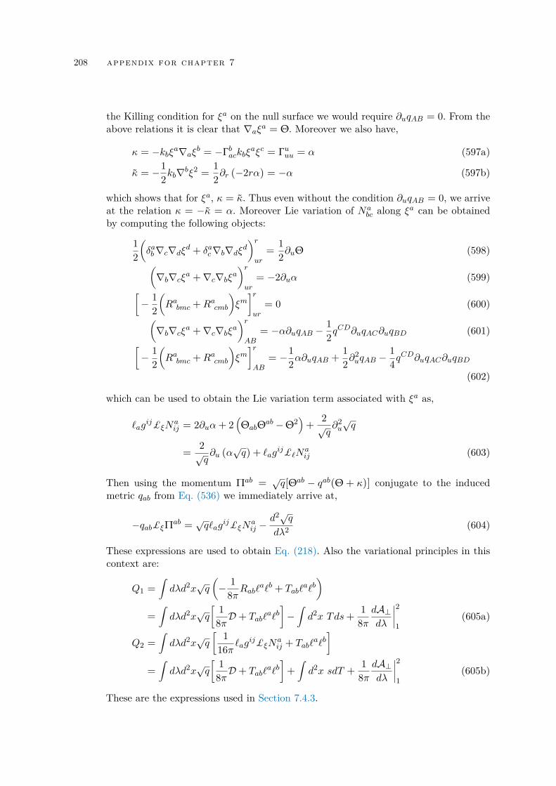
208 appendix for chapter 7

the Killing condition for ξa on the null surface we would require ∂uqAB = 0. From theabove relations it is clear that ∇aξa = Θ. Moreover we also have,

κ = −kbξa∇aξb = −Γbackbξaξc = Γuuu = α (597a)

κ = −12kb∇

bξ2 =12∂r (−2rα) = −α (597b)

which shows that for ξa, κ = κ. Thus even without the condition ∂uqAB = 0, we arriveat the relation κ = −κ = α. Moreover Lie variation of Na

bc along ξa can be obtainedby computing the following objects:

12

(δab∇c∇dξd + δac∇b∇dξd

)rur

=12∂uΘ (598)(

∇b∇cξa +∇c∇bξa)rur

= −2∂uα (599)[− 1

2

(Rabmc +Racmb

)ξm]rur

= 0 (600)(∇b∇cξa +∇c∇bξa

)rAB

= −α∂uqAB −12q

CD∂uqAC∂uqBD (601)[− 1

2

(Rabmc +Racmb

)ξm]rAB

= −12α∂uqAB +

12∂

2uqAB −

14q

CD∂uqAC∂uqBD

(602)

which can be used to obtain the Lie variation term associated with ξa as,

`agij£ξN

aij = 2∂uα+ 2

(ΘabΘab −Θ2

)+

2√q∂2u

√q

=2√q∂u (α

√q) + `ag

ij£`Naij (603)

Then using the momentum Πab =√q[Θab − qab(Θ + κ)] conjugate to the induced

metric qab from Eq. (536) we immediately arrive at,

−qab£ξΠab =√q`ag

ij£ξNaij −

d2√qdλ2 (604)

These expressions are used to obtain Eq. (218). Also the variational principles in thiscontext are:

Q1 =∫dλd2x

√q

(− 1

8πRab`a`b + Tab`

a`b)

=∫dλd2x

√q

[ 18πD+ Tab`

a`b]−∫d2x Tds+

18π

dA⊥dλ

∣∣∣∣21

(605a)

Q2 =∫dλd2x

√q

[ 116π`ag

ij£ξNaij + Tab`

a`b]

=∫dλd2x

√q

[ 18πD+ Tab`

a`b]+∫d2x sdT +

18π

dA⊥dλ

∣∣∣∣21

(605b)

These are the expressions used in Section 7.4.3.

EAPPENDIX FOR CHAPTER 8

For the sake of completeness, we derive the bracket for the Noether charge associatedwith the vectors as given in Eq. (250).

The normalized normal to r = constant surface corresponds to,

Na =

(0, 1√

2rα+ r2β2 , 0, 0)

(606)

Na =

(1√

2rα+ r2β2 ,√

2rα+ r2β2, rβA√2rα+ r2β2

)(607)

The extrinsic curvature of the r = 0 surface can be computed easily using the abovenormalized normal Na as,

K = −∇aNa = −∂aNa −Na∂a ln√−g

= −∂u

(1√

2rα+ r2β2

)− ∂r

√2rα+ r2β2

= − α√2rα+ r2β2 (608)

The corresponding non-zero component of the Noether potential associated with theNoether charge on r = 0 surface yield,

Jur = Kξunr −Kξrnu

= −(α− ∂uα

2α

)(F +

∂uF

2α

)(609)

Finally the relevant component of the Noether current for calculation of the bracketbetween Noether charges becomes

Jr = ∂uJru + ∂AJ

rA + JrA∂A ln√−g

= ∂u

[α

(F +

∂uF

2α

)]= α∂uF +

12∂

2uF (610)

The other normalized vector (the time evolution vector) corresponds to,

Ma =

( 1√2rα

, 0, 0, 0)

(611)

Ma =

(−√

2rα, 1√2rα

,− rβA√2rα

)(612)

209

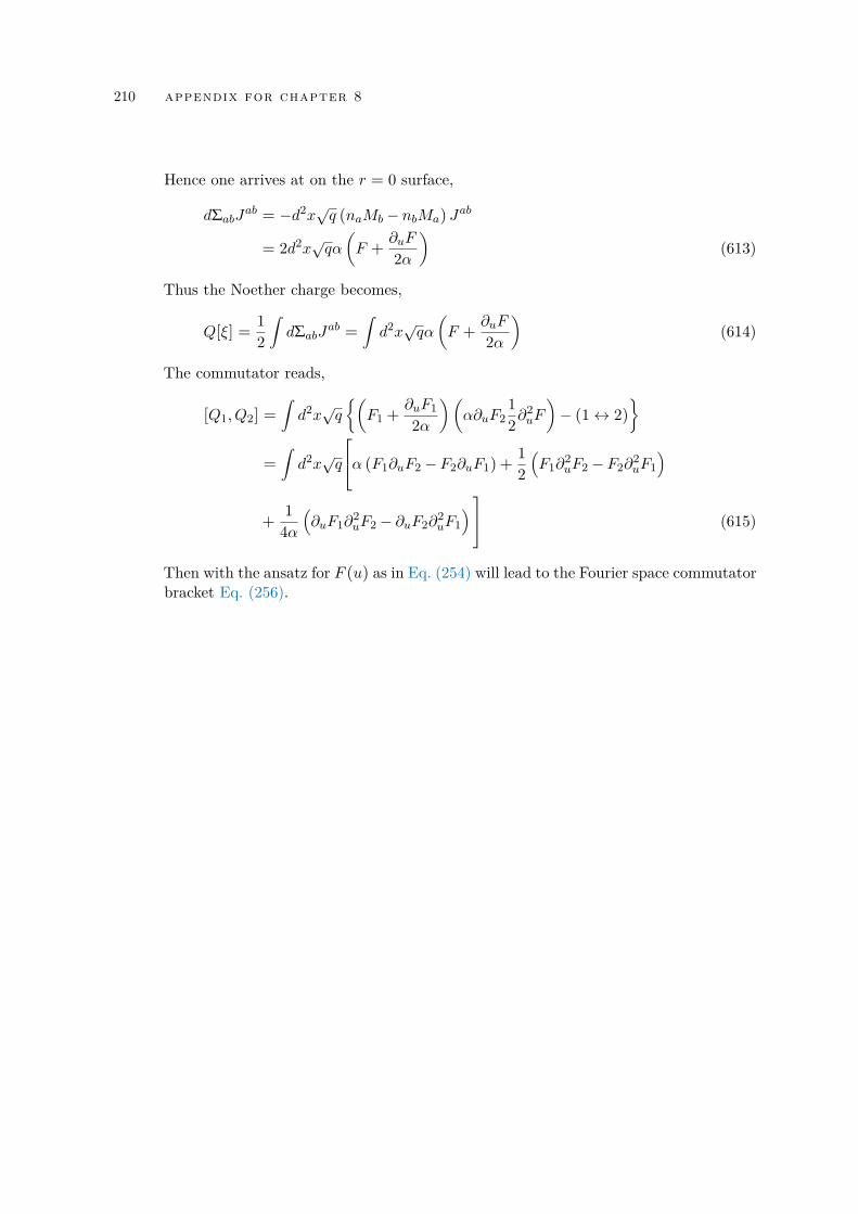
210 appendix for chapter 8

Hence one arrives at on the r = 0 surface,

dΣabJab = −d2x√q (naMb − nbMa) J

ab

= 2d2x√qα

(F +

∂uF

2α

)(613)

Thus the Noether charge becomes,

Q[ξ] =12

∫dΣabJab =

∫d2x√qα

(F +

∂uF

2α

)(614)

The commutator reads,

[Q1,Q2] =∫d2x√q

(F1 +

∂uF12α

)(α∂uF2

12∂

2uF

)− (1↔ 2)

=∫d2x√q

α (F1∂uF2 − F2∂uF1) +12(F1∂

2uF2 − F2∂

2uF1

)

+1

4α(∂uF1∂

2uF2 − ∂uF2∂

2uF1

) (615)

Then with the ansatz for F (u) as in Eq. (254) will lead to the Fourier space commutatorbracket Eq. (256).

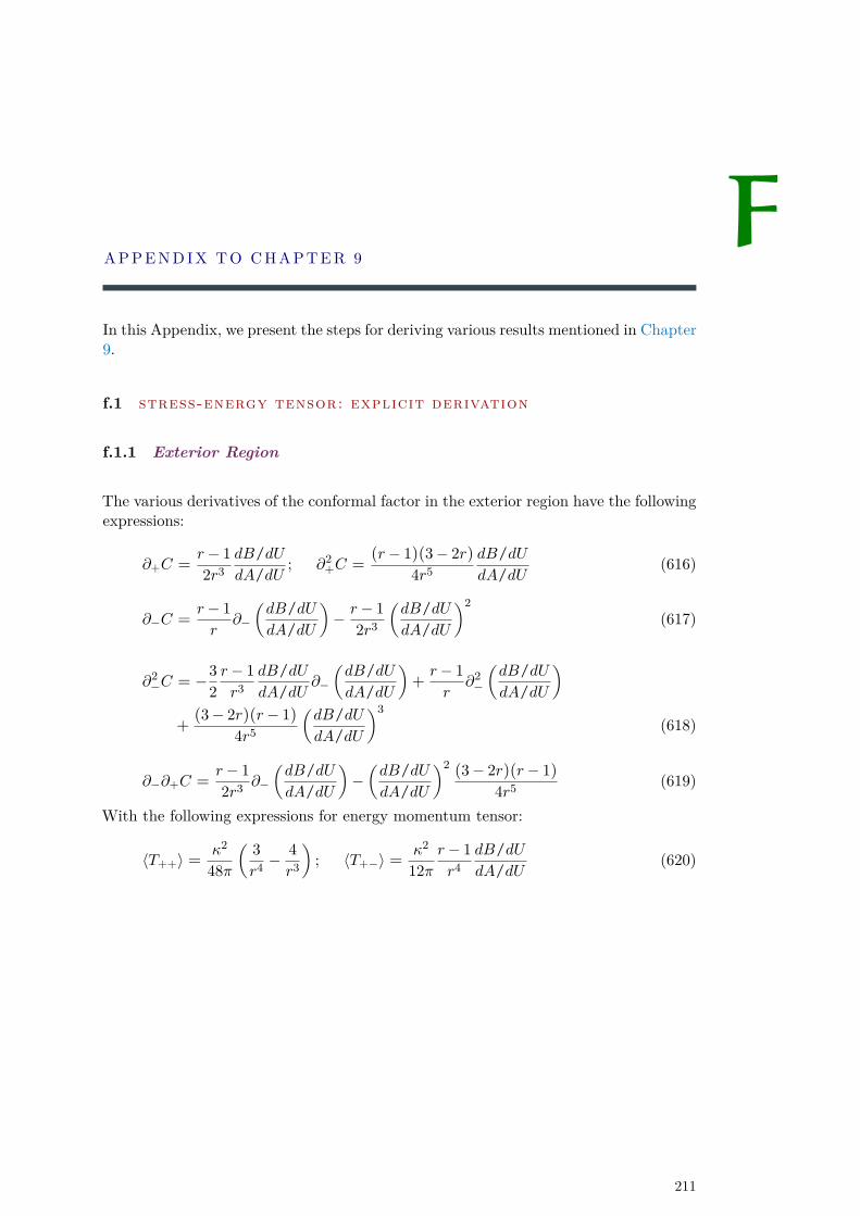
FAPPENDIX TO CHAPTER 9

In this Appendix, we present the steps for deriving various results mentioned in Chapter9.

f.1 stress-energy tensor: explicit derivation

f.1.1 Exterior Region

The various derivatives of the conformal factor in the exterior region have the followingexpressions:

∂+C =r− 12r3

dB/dUdA/dU

; ∂2+C =

(r− 1)(3− 2r)4r5

dB/dUdA/dU

(616)

∂−C =r− 1r

∂−

(dB/dUdA/dU

)− r− 1

2r3

(dB/dUdA/dU

)2(617)

∂2−C = −3

2r− 1r3

dB/dUdA/dU

∂−

(dB/dUdA/dU

)+r− 1r

∂2−

(dB/dUdA/dU

)+

(3− 2r)(r− 1)4r5

(dB/dUdA/dU

)3(618)

∂−∂+C =r− 12r3 ∂−

(dB/dUdA/dU

)−(dB/dUdA/dU

)2 (3− 2r)(r− 1)4r5 (619)

With the following expressions for energy momentum tensor:

〈T++〉 =κ2

48π

( 3r4 −

4r3

); 〈T+−〉 =

κ2

12πr− 1r4

dB/dUdA/dU

(620)

211

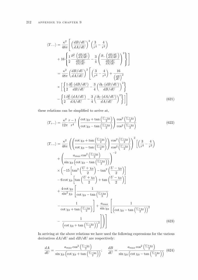
212 appendix to chapter 9

〈T−−〉 =κ2

48π

(dB/dUdA/dU

)2 ( 3r4 −

4r3

)

+ 16

12∂2−

(dB/dUdA/dU

)dB/dUdA/dU

− 34

∂−(dB/dUdA/dU

)dB/dUdA/dU

2

=κ2

48π

(dB/dUdA/dU

)2( 3

r4 −4r3

)+

16(dBdU

)2

×[1

2∂2U (dB/dU)dB/dU

− 34

(∂U (dB/dU)dB/dU

)2

−

12∂2U (dA/dU)dA/dU

− 34

(∂U (dA/dU)dA/dU

)2] (621)

these relations can be simplified to arrive at,

〈T+−〉 =κ2

12πr− 1r4

cotχ0 + tan(U−χ0

2

)cotχ0 − tan

(U+χ0

2

) cos2

(U+χ0

2

)cos2

(U−χ0

2

) (622)

〈T−−〉 =κ2

48π

cotχ0 + tan(U+χ0

2

)cotχ0 − tan

(U+χ0

2

) cos2

(U+χ0

2

)cos2

(U−χ0

2

)2 [( 3

r4 −4r3

)

+

amax cos2(U+χ0

2

)sinχ0

(cotχ0 − tan

(U+χ0

2

))−2

×(−15

[tan2

(U + χ0

2

)− tan2

(U − χ0

2

)]− 6 cotχ0

[tan

(U + χ0

2

)+ tan

(U − χ0

2

)]

+4 cotχ0sin2 χ0

1cotχ0 − tan

(U+χ0

2

)− 1

cotχ0 + tan(U−χ0

2

)+ amax

sinχ0

1(cotχ0 − tan

(U+χ0

2

))2

− 1(cotχ0 + tan

(U−χ0

2

))2

(623)

In arriving at the above relations we have used the following expressions for the variousderivatives dA/dU and dB/dU are respectively:

dA

dU=

amax cos2(U−χ0

2

)sinχ0

(cotχ0 + tan

(U−χ0

2

)) ; dB

dU=

amax cos2(U+χ0

2

)sinχ0

(cotχ0 − tan

(U+χ0

2

)) (624)

F.1 stress-energy tensor: explicit derivation 213

d2A

dU2 = −12

[1 + 2 sin2

(U−χ0

2

)+ cotχ0 sin (U − χ0)

]sin4 χ0

(cotχ0 + tan

(U−χ0

2

))2 (625)

d2B

dU2 =12

[1 + 2 sin2

(U+χ0

2

)− cotχ0 sin (U + χ0)

]sin4 χ0

(cotχ0 − tan

(U+χ0

2

))2 (626)

as well as the following derivatives:

12∂2U (dA/dU)dA/dU

− 34

(∂U (dA/dU)dA/dU

)2= − 1

16

[15 tan4

(U − χ0

2

)+ 24 cotχ0 tan3

(U − χ0

2

)+ 10 tan2

(U − χ0

2

)+ 4 cot2 χ0

1 + 2 tan2

(U − χ0

2

)+ 16 cotχ0 tan

(U − χ0

2

)− 1

] [cotχ0 + tan

(U − χ0

2

)]−2

= − 116

[15 tan2

(U − χ0

2

)− 6 cotχ0 tan

(U − χ0

2

)+ 5

(1 + sin−2 χ0

)− 4 sin−2 χ0 cotχ0

cotχ0 + tan(U−χ0

2

) − amax

sinχ0(cotχ0 + tan

(U−χ0

2

))2

](627)

and

12∂2U (dB/dU)dB/dU

− 34

(∂U (dB/dU)dB/dU

)2= − 1

16

[15 tan4

(U + χ0

2

)− 24 cotχ0 tan3

(U + χ0

2

)− 10 tan2

(U + χ0

2

)+ 4 cot2 χ0

1 + 2 tan2

(U + χ0

2

)− 16 cotχ0 tan

(U + χ0

2

)− 1

] [cotχ0 − tan

(U + χ0

2

)]−2

= − 116

[15 tan2

(U + χ0

2

)+ 6 cotχ0 tan

(U + χ0

2

)+ 5

(1 + sin−2 χ0

)− 4 sin−2 χ0 cotχ0

cotχ0 − tan(U+χ0

2

) − amax

sinχ0(cotχ0 − tan

(U+χ0

2

))2

](628)

f.1.2 Interior Region

For the interior region the various derivatives of the conformal factors are:

1C∂+C =

1(dA/dV )

[1a2da2

dV− d2A/dV 2

dA/dV

]1C∂−C =

1(dA/dU)

[1a2da2

dU− d2A/dU2

dA/dU

](629)

214 appendix to chapter 9

1C∂2+C =

1(dA/dV )2

1a2d2a2

dV 2 −3a2da2

dV

1dA/dV

d2A

dV 2

− 1dA/dV

d3A

dV 3 + 3(

1dA/dV

d2A

dV 2

)2 (630)

1C∂2−C =

1(dA/dU)2

1a2d2a2

dU2 −3a2da2

dU

1dA/dU

d2A

dU2 −1

dA/dUd3A

dU3

+ 3(

1dA/dU

d2A

dU2

)2 (631)

1C∂−∂+C =

1dAdV

dAdU

[1a2

d2a2

dUdV− 1a2da2

dU

1dA/dV

d2A

dV 2 −1a2da2

dV

1dA/dU

d2A

dU2

+1

dA/dVd2A

dV 21

dA/dUd2A

dU2

](632)

Then the components of the stress energy tensor in the inside region are:

〈T++〉 =1

12π1

(dA/dV )2

12a2

d2a2

dV 2 −34

(1a2da2

dV

)2−

12

1dA/dV

d3A

dV 3

−34

1(dA/dV )2

(d2A

dV 2

)2

=1

12π1

(dA/dV )2

− 18

3amax sinχ0

r(U+V

2

) − 2

−

12∂2V (dA/dV )

(dA/dV )− 3

4

(∂V (dA/dV )

(dA/dV )

)2 (633)

〈T−−〉 =1

12π1

(dA/dU)2

12a2

d2a2

dU2 −34

(1a2da2

dU

)2−

12

1dA/dU

d3A

dU3

−34

1(dA/dU)2

(d2A

dU2

)2

=1

12π1

(dA/dU)2

−18

3amax sinχ0

r(U+V

2

) − 2

−12∂2U (dA/dU)(dA/dU)

−34

(∂U (dA/dU)(dA/dU)

)2](634)

F.2 energy density and flux for various observers 215

〈T+−〉 =1

24π1

dA/dV1

dA/dU

[1a2

d2a2

dUdV− 1a2da2

dU

1a2da2

dV

]

= − 148π

1dA/dV

1dA/dU

11 + cos

(U+V

2

) (635)

where various derivatives of the quantity A are given in Appendix F.1.1.

f.2 energy density and flux for various observers

f.2.1 Static Observer

Below we provide the full expressions for energy density and flux calculated for staticobserver:

U = 〈T++〉(V +)2 + 〈T−−〉 (V −)2 + 2〈T+−〉V +V −

=κ2

48π

(r

r− 1

)[(− 2r4

)+

sin2 χ0

a2max cos4

(U+χ0

2

) (cotχ0 − tan(U + χ0

2

))2

×− 15

[tan2

(U + χ0

2

)− tan2

(U − χ0

2

)]− 6 cotχ0

[tan

(U + χ0

2

)+ tan

(U − χ0

2

)]

+4 cotχ0sin2 χ0

1cotχ0 − tan

(U+χ0

2

) − 1cotχ0 + tan

(U−χ0

2

)

+sinχ0

amax cos4(U+χ0

2

)1−

(cotχ0 − tan

(U+χ0

2

))2

(cotχ0 + tan

(U−χ0

2

))2

] (636)

and the expression for flux turns out to be:

F = −〈Tab〉uanb = −〈T++〉(V +)2 + 〈T−−〉 (V −)2

=κ2

48π

(r

r− 1

)[ sin2 χ0

a2max cos4

(U+χ0

2

) (cotχ0 − tan(U + χ0

2

))2

×− 15

[tan2

(U + χ0

2

)− tan2

(U − χ0

2

)]− 6 cotχ0

[tan

(U + χ0

2

)+ tan

(U − χ0

2

)]

+4 cotχ0sin2 χ0

1cotχ0 − tan

(U+χ0

2

) − 1cotχ0 + tan

(U−χ0

2

)

+sinχ0

amax cos4(U+χ0

2

)1−

(cotχ0 − tan

(U+χ0

2

))2

(cotχ0 + tan

(U−χ0

2

))2

] (637)

216 appendix to chapter 9

f.2.2 Radially In-falling Observers: Inside

The energy density for radially in-falling observer has the following expression:

U =κ2

48π1

a2 (η)

[− 8 sec2 η

2 + 4 + 12

15 tan2

(η− χ0 − χ

2

)− 6 cotχ0 tan

(η− χ0 − χ

2

)+ 5

(1 + sin−2 χ0

)− 4 sin−2 χ0 cotχ0

cotχ0 + tan(η−χ0−χ

2

) − amax

sinχ0(cotχ0 + tan

(η−χ0−χ

2

))2

+ 15 tan2(η− χ0 + χ

2

)− 6 cotχ0 tan

(η− χ0 + χ

2

)+ 5

(1 + sin−2 χ0

)− 4 sin−2 χ0 cotχ0

cotχ0 + tan(η−χ0+χ

2

) − amax

sinχ0(cotχ0 + tan

(η−χ0+χ

2

))2

](638)

while the flux has the following expression:

F =κ2

48π1

a2 (η)

12

15 tan2

(η− χ0 − χ

2

)− 6 cotχ0 tan

(η− χ0 − χ

2

)+ 5

(1 + sin−2 χ0

)− 4 sin−2 χ0 cotχ0

cotχ0 + tan(η−χ0−χ

2

)− amax

sinχ0(cotχ0 + tan

(η−χ0−χ

2

))2 − 15 tan2(η− χ0 + χ

2

)

+ 6 cotχ0 tan(η− χ0 + χ

2

)− 5

(1 + sin−2 χ0

)+

4 sin−2 χ0 cotχ0

cotχ0 − tan(η−χ0+χ

2

) +amax

sinχ0(cotχ0 + tan

(η−χ0+χ

2

))2

(639)

F.2 energy density and flux for various observers 217

f.2.3 Radially In-falling Observers: Outside

For radially in-falling observer outside the dust ball has the following expression forenergy density:

U = 〈T++〉(V +)2 + 〈T−−〉 (V −)2 + 2〈T+−〉V +V −

=κ2

48π4E2(

r

r− 1

)2 ( 3r4 −

4r3

)+

κ2

24π

(r

r− 1

)(− 7r4 +

8r3

)

+κ2

48π

(r

r− 1

)2(E +

√E2 − r− 1

r

)2

×[ sin2 χ0

a2max cos4

(η+χ0−χ

2

) (cotχ0 − tan(η+ χ0 − χ

2

))2

×− 15

[tan2

(η+ χ0 − χ

2

)− tan2

(η− χ0 − χ

2

)]− 6 cotχ0

[tan

(η+ χ0 − χ

2

)+ tan

(η− χ0 − χ

2

)]

+4 cotχ0sin2 χ0

1cotχ0 − tan

(η+χ0−χ

2

) − 1cotχ0 + tan

(η−χ0−χ

2

)

+sinχ0

amax cos4(η+χ0−χ

2

)1−

(cotχ0 − tan

(η+χ0−χ

2

))2

(cotχ0 + tan

(η−χ0−χ

2

))2

] (640)

and the flux has the following expression:

F = −〈Tab〉uanb = −〈T++〉(V +)2 + 〈T−−〉 (V −)2

=κ2

48π4E√E2 − r− 1

r

(r

r− 1

)2 ( 3r4 −

4r3

)+

κ2

48π

(r

r− 1

)2

×(E +

√E2 − r− 1

r

)2 [ sin2 χ0

a2max cos4

(η+χ0−χ

2

) (cotχ0 − tan(η+ χ0 − χ

2

))2

×− 15

[tan2

(η+ χ0 − χ

2

)− tan2

(η− χ0 − χ

2

)]− 6 cotχ0

[tan

(η+ χ0 − χ

2

)+ tan

(η− χ0 − χ

2

)]

+4 cotχ0sin2 χ0

1cotχ0 − tan

(η+χ0−χ

2

) − 1cotχ0 + tan

(η−χ0−χ

2

)

+sinχ0

amax cos4(η+χ0−χ

2

)1−

(cotχ0 − tan

(η+χ0−χ

2

))2

(cotχ0 + tan

(η−χ0−χ

2

))2

] (641)

218 appendix to chapter 9

f.3 effective temperature for various observers

In this section we present the full expression for effective temperature measured bydetectors in various trajectories. For static observer the effective temperature turns outto be:

T− =1

2π

∣∣∣∣∣ V −V −∣∣∣∣∣

=1

2π

∣∣∣∣∣∣∣u d2A

dU2

dAdU

dBdU

−d2BdU2(dBdU

)2

∣∣∣∣∣∣∣

=1

4π

√r

r− 1 sin4 χ0

×[1 + 2 sin2

(U−χ0

2

)+ cotχ0 sin (U − χ0)

] (cotχ0 − tan

(U+χ0

2

))(cotχ0 + tan

(U−χ0

2

))cos2

(U+χ0

2

)cos2

(U−χ0

2

)+

[1 + 2 sin2

(U+χ0

2

)− cotχ0 sin (U + χ0)

]cos4

(U+χ0

2

) (642)

For radially in-falling observes inside the dust sphere the effective temperature turnsout to be:

T− =1

4π

∣∣∣∣∣∣1 + 2 sin2

(η−χ0−χ

2

)+ cotχ0 sin

(η−χ0−χ

2

)cos2

(η−χ0−χ

2

)cotχ0 + tan

(η−χ0−χ

2

)∣∣∣∣∣∣ (643)

Finally, for radially in-falling observers in the Schwarzschild spacetime effective tem-perature takes the following expression:

T− =1

2π

∣∣∣∣∣∣ uu − usin4 χ02

[1 + 2 sin2(η−χ0−χ

2

)+ cotχ0 sin (η− χ0 − χ)

] (cotχ0 − tan

(η+χ0−χ

2

))(cotχ0 + tan

(η−χ0−χ

2

))cos2

(η+χ0−χ

2

)cos2

(η−χ0−χ

2

)+

[1 + 2 sin2

(η+χ0−χ

2

)− cotχ0 sin (η+ χ0 − χ)

]cos4

(η+χ0−χ

2

) ∣∣∣∣∣∣ (644)

GAPPENDIX FOR CHAPTER 10

g.1 spectrum operator

Using the expression for the correction term over the vacuum thermal spectrum, wecan obtain the distortion from thermal Hawking radiation for one particle initial stateof the field which is undergoing the collapse as,

NΩ =

[∣∣∣∣∫ ∞0

dω′√4πω′

α∗Ωω′f(ω′)

∣∣∣∣2 + ∣∣∣∣∫ ∞0

dω√4πω

βΩωf(ω)

∣∣∣∣2]

. (645)

It must be noted that the expression in Eq. (645) is general enough to include caseswhen the Bogoliubov coefficients as in Eq. (327) are modified by back-reaction, angularmomentum, quantum gravity etc. In any case, the non-vacuum part of the radiationspectra provides a constraint for f(ω) in form of Eq. (645). Using Eq. (332), we canrewrite Eq. (645) as

NΩ =1

4π1

4πκ1

sinh πΩκ

[∣∣∣∣F (Ωκ

)∣∣∣∣2 + ∣∣∣∣F (−Ωκ

)∣∣∣∣2]

. (646)

We can decompose |F (Ω/κ) |2 into symmetric S (Ω/κ) and an anti-symmetric partA (Ω/κ) ∣∣∣∣F (Ω

κ

)∣∣∣∣2 = S

(Ωκ

)+ A

(Ωκ

). (647)

With this decomposition, we realize from Eq. (646) that the symmetric part of |F (Ω/κ) |2is entirely characterized by the distribution function NΩ of the radiation,

S

(Ωκ

)= 8π2κNΩ sinh πΩ

κ. (648)

Further, if the in-state is normalized to unity, we have∫ ∞−∞

d

(Ωκ

)e−

πΩκ

[S

(Ωκ

)+ A

(Ωκ

)]= 8π2, (649)

which together with Eq. (648) regulates the integral (and hence the asymptotic behav-ior) of A (κ). Apart from this constraint, A (κ) is a completely arbitrary anti-symmetricfunction. Therefore, the radiation spectra fixes the symmetric part of the probabilitydensity in the Fourier space corresponding to z. However, the anti-symmetric part ofthis probability density remains largely unspecified.

219

220 appendix for chapter 10

In terms of the function g(z) defined in Eq. (333), the symmetric part S(

Ωκ

)can be

written as

eπΩκ ×

∫ ∞−∞

dy

∫ ∞−∞

dzg(z − y/2)g∗(z + y/2)e−iΩκy

+ e−πΩκ

∫ ∞−∞

dy

∫ ∞−∞

dzg(z − y/2)g∗(z + y/2)eiΩκy = 2S

(Ωκ

). (650)

As, we see that F (κ) is “momentum space representation" conjugate to g(z), the aboveexpression can be written in terms of the Wigner function corresponding to the phasespace of (z, Ω/κ),

eπΩκ

∫ ∞−∞

dzWg

(z, Ωκ

)+ e−π

Ωκ

∫ ∞−∞

dzWg

(z,−Ω

κ

)= 2S

(Ωκ

), (651)

where the Wigner function is defined as,

Wg

(z, Ωκ

)=∫ ∞−∞

dyg(z − y/2)g∗(z + y/2)e−iΩκy. (652)

Also, with the relation ∣∣∣∣F (Ωκ

)∣∣∣∣2 =∫ ∞−∞

dzWg

(z, Ωκ

), (653)

we obtain,

eπΩκ

∣∣∣∣F (Ωκ

)∣∣∣∣2 + e−πΩκ

∣∣∣∣F (−Ωκ

)∣∣∣∣2 = 2S(

Ωκ

), (654)

which is an obvious illustration of Eq. (648). Therefore, integrating the relation Eq. (654)over the frequency range at J + we obtain the relation

2∫ ∞

0d

(Ωκ

)S

(Ωκ

)=

∫ ∞0

d

(Ωκ

)eπΩκ

∫ ∞−∞

dzWg

(z, Ωκ

)+

∫ ∞0

d

(Ωκ

)e−

πΩκ

∫ ∞−∞

dzWg

(z,−Ω

κ

)=

∫ ∞−∞

dyeπy |F (y)|2 . (655)

Although, the state which would be completely specified, if we know F (y), remainsarbitrary apart form this constraint, the symmetric part S (Ω/κ) which is completelyspecified through the non-vacuum distortion, fixes the expectation of the exponentiatedmomenta conjugate to z(= logω/C).

For a n-particle state

|Ψ〉 =∫ ∞

0

n∏i=1

dωi√2πωi

f(ω1, ...ωn)a†(ωi)|0〉M , (656)

G.1 spectrum operator 221

the radiation profile over the thermal component fixes the expectation of a single par-ticle exponentiated momentum, i.e.,

16∫ ∞

0d

(Ωκ

)π2κ

(sinh πΩ

κ

)NΩ =

1n〈Ψ|e

πΩκ |Ψ〉. (657)

Additional information about the initial state can only be obtained from the spectrum ifthe initial state has some symmetries. We will discuss few interesting cases below.

• If F (y) is a real and symmetric function, then we see from Eq. (654) that it getscompletely specified in terms of S(Ω/κ). As, a result the initial state also getscompletely specified as g(z) can be obtained by the inverse Fourier transform.However, by virtue of the properties of Fourier transform, g(z) also happens tobe real and symmetric. This symmetry corresponds to a duality in the frequencyspace distribution about the surface gravity parameter κ. These states are veryspecial class of initial states whose information get coded entirely in the radiationfrom the black hole within the framework of standard unitary quantum mechanics.

• For a slightly more general case, the reality condition on g(z) can be traded forby imposing relation between F (Ω/κ) and F (−Ω/κ), which is to specify thesymmetry of F (y) in the positive and negative half planes. Such a specificationof symmetry constrains the distribution F (y) to remain arbitrary in one of thehalf planes and amounts to reducing the degrees of freedom by half. Let us assumeF (Ω/κ) is real, that means

g(z) = g∗(−z). (658)

Now additionally if we impose,

F (−y) = K (y)F (y) , (659)

for a specified function K(y), then∫ ∞−∞

dzg(z)e−iyz =∫ ∞−∞

dzg(z)eiyzK (y) . (660)

Therefore, using the condition Eq. (658), we can obtain from Eq. (660)

g∗(z) =∫ ∞−∞

dz′g(z′)∫ ∞−∞

dyK (y) eiy(z′−z)

=∫ ∞−∞

dz′g(z′)K(z′ − z), (661)

where K(q) is the inverse Fourier transform of K(y). Therefore, for such a sym-metry in the probability amplitude, the state can be recovered from

F 2(

Ωκ

)= 16π2κ

(sinh πΩ

κ

)eπΩκ +

(K(

Ωκ

))2e−

πΩκ

NΩ. (662)

Therefore, we see that the symmetry of the prescribed class for one particle sate encodesthe entire information of the in-state in the resulting radiation from the black hole. If

222 appendix for chapter 10

the initial condition of the collapse demands symmetry of such kinds, the resultingmixed state has enough information in the spectra to completely specify the state. Wewill further consider some other classes of symmetries in the initial data for sphericallysymmetric collapse models and their imprints in the non-vacuum distortions.

g.2 real initial distribution

For real distributions, the Fourier transform will satisfy

|F (y)|2 = |F (−y)|2 (663)

Therefore, |K(y)| = 1 and we have the relation∣∣∣∣F (Ωκ

)∣∣∣∣2 + ∣∣∣∣F (−Ωκ

)∣∣∣∣2 = 8π2κ tanh πΩκNΩ. (664)

For a symmetric algebraic operator of y

Oeven(y) = Oeven(−y), (665)

the expression

8π2κ × tanh πΩκOeven

(Ωκ

)NΩ

= Oeven

(Ωκ

) ∣∣∣∣F (Ωκ

)∣∣∣∣2 +Oeven

(−Ωκ

) ∣∣∣∣F (−Ωκ

)∣∣∣∣2 (666)

which on integration over the whole frequency range gives the expectation value of theoperator

∫ ∞0

d

(Ωκ

)8π2κ tanh πΩ

κOeven

(Ωκ

)NΩ =

∫ ∞0

d

(Ωκ

)Oeven

(Ωκ

) ∣∣∣∣F (Ωκ

)∣∣∣∣2

+ Oeven

(−Ωκ

) ∣∣∣∣F (−Ωκ

)∣∣∣∣2

=∫ ∞−∞Oeven(y)|F (y)|2. (667)

By similar logic, one can argue that expectation of all odd algebraic operators vanishin this case, i.e., with a symmetric |F (y)|2,the expectation value for an odd observ-able

〈Oodd(y)〉 =∫ ∞−∞

dyOodd(y)|F (y)|2 = 0. (668)

Thus in this scenario, expectation of all algebraic operators in y will be given in termsof spectral distortion. Any general operator O(y) can be decomposed in terms of itseven and odd parts

O(y) = Oeven(y) + Oodd(y). (669)

G.3 state for step function support 223

Therefore, to obtain 〈O(y)〉 one only requires 〈Oeven(y)〉, which can be easily obtainedfrom Eq. (667). Similarly for the generalized symmetry class

〈O(y)〉 =∫ ∞

0dy[O (y) |F (y)|2 +O (−y) |F (−y)|2

]=∫ ∞

0dy(O (y) + |K(y)|2O (−y)) |F (y)|2

= 16π2κ

∫ ∞0

dΩ[O (Ω) + |K(Ω)|2O (−Ω)] sinh Ω

eπΩκ +

∣∣K (Ω)∣∣2 e−πΩ

κ

NΩ,

(670)

where we have used the expression of |F (y)|2 in the range y ∈ (0,∞) from Eq. (662), inthe third equality. Thus even with the specified symmetry class K(y), all the algebraicoperators on the momentum space become fixed.

g.3 state for step function support

Let us excite some right-moving modes beyond x+i (for simplicity we work with singleparticle states), such that the normal ordered operator T++(x+) has support only inthe region inside the horizon, i.e.,

〈T++(x+)〉Regularized = h(x+)Θ(x+ − x+i ), (671)

for some well behaved function h(x+) and the step function Θ(x+).

If the single particle state is taken to be in the frame of observers which would havedescribed the linear dilaton vacuum, then

|Ψ〉 =∫ωf(ω)a†ω|0〉, (672)

where∫ω stands for

∫dω/√

4πω and the right-moving quantum field is given on J +L

as

f+(y+) =

∫ω(aωuω(y

+) + a†ωu∗ω(y

+)), (673)

with mode functions uω(y+). Then the equation Eq. (671) can be re-written as∣∣∣∣∫ωf(ω)u′ω(y

+)

∣∣∣∣2 = h1(y+)Θ(y+ − y+i ), (674)

where ′ denotes a derivative with respect to y+ and y+i marking the location corre-sponding to x+i . The function h1(y+) absorbs the Jacobian of transformation from x±

basis to y± basis,

T++(x+) =

∂yµ

∂x+∂yν

∂x+Tµν(y

+) =∂y+

∂x+∂y+

∂x+T++(y

+) (675)

224 appendix for chapter 10

The condition Eq. (674) can be realized by∫ωf(ω)u′ω(y

+) = h(y+)Θ(y+ − y+i ), (676)

with some other well behaved function h(y+). Owing to the conformal flatness of thetwo dimensional spacetime and the conformal nature of minimally coupled masslessscalar field, the mode functions can be written as

u′ω(y+) = −iωuω(y+). (677)

Therefore, we only require to have∫ωf(ω)ωuω(x

+) = h(x+)Θ(x+ − x+i ) = ζ(x+), (678)

where we have absorbed the factor i in the redefinition of h(x+). Taking the innerproduct of the Eq. (678) with itself and using the orthonormal properties of the modefunctions, we write ∫

ωω2|f(ω)|2 = (ζ(x+), ζ(x+)). (679)

For the states satisfying Eq. (679), the expression Eq. (678) can be inverted for givenζ(x+), using the completeness of mode functions to obtain a consistent state. Therefore,the one particle states respecting Eq. (679) will have mode excitations beyond x+i .

g.4 information retrieval for the cghs black hole

Using a particular representation of the Gamma function

Γ[z] = iz∫ ∞−∞

dqezqe−ieq , (680)

we can write down a product formula

Γ[i(ω− ω′)]Γ[−i(ω− ω′′)] = e−πωeπ2 (ω′+ω′′)

×∫ ∞−∞

dq1dq2eiω(q1−q2)ei(ω

′q1−ω′′q2)e−ieq1+ieq2 , (681)

which appears in the spectrum operator expression. The correction in the vacuumthermal radiation as received by asymptotic left moving observer can be expressedas

2πλ sinh πωNω =∫ ∞

0

∫ ∞0

dω′

ω′dω′′

ω′′Symω

[Γ[i(ω− ω′)]Γ[−i(ω− ω′′)]

Γ[−iω′]Γ[iω′′]

]×∣∣y+i ∣∣i(ω′−ω′′) f(ω′)f∗(ω′′), (682)

G.4 information retrieval for the cghs black hole 225

where Symx[f(x)] = (f(x) + f(−x))/2 with ω′ = ω′/λ. Using Eq. (371), the spectraldistortion can be re-written as,

2πλ sinh πωNω =∫ ∞

0dω′dω′′

∫ ∞−∞

dq1dq2Symω[e−πωeiω(q1−q2)]

× ei(ω′q1−ω′′q2)e−ieq1+ieq2

g(ω′)g∗(ω′′). (683)

Using, g(ω), introduce yet another function

χ(q) = e−ieq∫ ∞

0dωe−iωqg(ω), (684)

to express the spectral distortion as

2πλ sinh πωNω =∫ ∞−∞

dq1dq2Symω[e−πωeiω(q1−q2)]χ(q1)χ

∗(q2). (685)

4πλ sinh πωNω =∫ ∞−∞

dq1dq2[e−πωeiω(q1−q2) + eπωe−iω(q1−q2)]χ(q1)χ

∗(q2), (686)

which simply gives

4πλ sinh πωNω = eπω|Fχ(ω)|2 + e−πω|Fχ(−ω)|2, (687)

with Fχ(ω) being the Fourier transform of χ(q) w.r.t. ω

Fχ(ω) =∫ ∞−∞

dqe−iωqχ(q), (688)

which gives Eq. (687) as the analogue of the Eq. (654) for the spherical symmetriccollapse. Therefore, we can follow the same steps as outlined in Section 10.3 and Sec-tion 10.4 to recover informations regarding Fχ(ω). Using the inverse transformationsEq. (688), Eq. (684) and Eq. (371) we can recover the information regarding the fieldstate f(ω) using the moments of Fχ(ω).

BIBL IOGRAPHY

[1] Acquaviva, G., G. F. R. Ellis, R. Goswami, and A. I. M. Hamid (2015), Phys.Rev.D91 (6), 064017, arXiv:1411.5708 [gr-qc] .

[2] Adami, C., and G. L. Ver Steeg (2014), Class. Quant. Grav. 31, 075015, arXiv:gr-qc/0407090 [gr-qc] .

[3] Adler, S. L., and A. C. Millard (1996), Nucl. Phys. B473, 199, arXiv:hep-th/9508076 [hep-th] .

[4] Akbar, M., and R.-G. Cai (2006), Phys.Lett. B635, 7, arXiv:hep-th/0602156[hep-th] .

[5] Akhmedov, E. T., H. Godazgar, and F. K. Popov (2016), Phys. Rev. D93 (2),024029, arXiv:1508.07500 [hep-th] .

[6] Albers, M., C. Kiefer, and M. Reginatto (2008), Phys.Rev. D78, 064051,arXiv:0802.1978 [gr-qc] .

[7] Alves, M. (1995), arXiv:gr-qc/9510021 [gr-qc] .

[8] Alves, M. (1999), Int. J. Mod. Phys. D8, 687, arXiv:hep-th/9909138 [hep-th] .

[9] Ambjorn, J., A. Goerlich, J. Jurkiewicz, and R. Loll (2013), arXiv:1302.2173[hep-th] .

[10] Ambjorn, J., J. Jurkiewicz, and R. Loll (2005), Phys. Rev. D72, 064014,arXiv:hep-th/0505154 [hep-th] .

[11] Ambjorn, J., J. Jurkiewicz, and R. Loll (2005), Phys. Rev. Lett. 95, 171301,arXiv:hep-th/0505113 [hep-th] .

[12] Anderson, P. R., W. A. Hiscock, and D. J. Loranz (1995), Phys. Rev. Lett. 74,4365, arXiv:gr-qc/9504019 [gr-qc] .

[13] Anderson, P. R., W. A. Hiscock, and D. A. Samuel (1993), Phys. Rev. Lett. 70,1739.

[14] Arkani-Hamed, N., S. Dimopoulos, and G. Dvali (1998), Phys.Lett. B429, 263,arXiv:hep-ph/9803315 [hep-ph] .

[15] Ashtekar, A., J. Baez, A. Corichi, and K. Krasnov (1998), Phys. Rev. Lett. 80,904, arXiv:gr-qc/9710007 [gr-qc] .

[16] Ashtekar, A., and A. Barrau (2015), arXiv:1504.07559 [gr-qc] .

[17] Ashtekar, A., and M. Bojowald (2005), Class. Quant. Grav. 22, 3349, arXiv:gr-qc/0504029 [gr-qc] .

227

228 bibliography

[18] Ashtekar, A., F. Pretorius, and F. M. Ramazanoglu (2011), Phys. Rev. Lett.106, 161303, arXiv:1011.6442 [gr-qc] .

[19] Audretsch, J., and R. Muller (1992), Phys. Rev. D45, 513.

[20] Banerjee, K., and A. Paranjape (2009), Phys.Rev. D80, 124006, arXiv:0909.4668[gr-qc] .

[21] Barbado, L. C., C. Barcelo, and L. J. Garay (2011), Class. Quant. Grav. 28,125021, arXiv:1101.4382 [gr-qc] .

[22] Barcelo, C., S. Liberati, S. Sonego, and M. Visser (2011), Phys.Rev. D83, 041501,arXiv:1011.5593 [gr-qc] .

[23] Bardeen, J. M., B. Carter, and S. Hawking (1973), Commun.Math.Phys. 31,161.

[24] Bassi, A., and G. C. Ghirardi (2003), Phys. Rept. 379, 257, arXiv:quant-ph/0302164 [quant-ph] .

[25] Bassi, A., K. Lochan, S. Satin, T. P. Singh, and H. Ulbricht (2013), Rev. Mod.Phys. 85, 471, arXiv:1204.4325 [quant-ph] .

[26] Bekenstein, J. (1972), Lett. Nuovo Cimento Soc. Ital. Fis. 4, 737.

[27] Bekenstein, J. D. (1973), Phys.Rev. D7, 2333.

[28] Bekenstein, J. D. (1974), Phys.Rev. D9, 3292.

[29] Bekenstein, J. D. (1975), Phys. Rev. D12, 3077.

[30] Bhattacharya, S. (2016), Eur. Phys. J. C76 (3), 112, arXiv:1506.07809 [gr-qc] .

[31] Birnir, B., S. B. Giddings, J. A. Harvey, and A. Strominger (1992), Phys. Rev.D46, 638, arXiv:hep-th/9203042 [hep-th] .

[32] Birrell, N., and P. Davies (1982), Cambridge Monogr.Math.Phys. .

[33] Bloete, H. W. J., J. L. Cardy, and M. P. Nightingale (1986), Phys. Rev. Lett.56, 742.

[34] Bodendorfer, N., T. Thiemann, and A. Thurn (2013), Class. Quant. Grav. 30,045001, arXiv:1105.3703 [gr-qc] .

[35] Bodendorfer, N., T. Thiemann, and A. Thurn (2013), Class. Quant. Grav. 30,045002, arXiv:1105.3704 [gr-qc] .

[36] Bodendorfer, N., T. Thiemann, and A. Thurn (2013), Class. Quant. Grav. 30,045003, arXiv:1105.3705 [gr-qc] .

[37] Bombelli, L., R. K. Koul, J. Lee, and R. D. Sorkin (1986), Phys. Rev. D34, 373.

[38] Boulware, D. G., and S. Deser (1985), Phys. Rev. Lett. 55, 2656.

[39] Brout, R., S. Massar, R. Parentani, and P. Spindel (1995), Phys.Rept. 260, 329,arXiv:0710.4345 [gr-qc] .

bibliography 229

[40] Cai, R.-G., and S. P. Kim (2005), JHEP 0502, 050, arXiv:hep-th/0501055 [hep-th] .

[41] Calcagni, G. (2010), Phys. Rev. Lett. 104, 251301, arXiv:0912.3142 [hep-th] .

[42] Calcagni, G., D. Oriti, and J. Thurigen (2013), Class. Quant. Grav. 30, 125006,arXiv:1208.0354 [hep-th] .

[43] Calcagni, G., D. Oriti, and J. ThÃŒrigen (2014), Class. Quant. Grav. 31, 135014,arXiv:1311.3340 [hep-th] .

[44] Callan, C. G., Jr., S. B. Giddings, J. A. Harvey, and A. Strominger (1992), Phys.Rev. D45, 1005, arXiv:hep-th/9111056 [hep-th] .

[45] Cardy, J. L. (1986), Nucl. Phys. B270, 186.

[46] Carlip, S. (1999), Class. Quant. Grav. 16, 3327, arXiv:gr-qc/9906126 [gr-qc] .

[47] Carlip, S. (2007), Gen. Rel. Grav. 39, 1519, [Int. J. Mod. Phys.D17,659(2008)],arXiv:0705.3024 [gr-qc] .

[48] Carlip, S. (2008), Class.Quant.Grav. 25, 154010, arXiv:0803.3456 [gr-qc] .

[49] Carlip, S. (2009), Proceedings, 25th Max Born Symposium: The Planck Scale,AIP Conf. Proc. 1196, 72, arXiv:0909.3329 [gr-qc] .

[50] Carlip, S. (2009), in Proceedings, Foundations of Space and Time: Reflections onQuantum Gravity, pp. 69–84, arXiv:1009.1136 [gr-qc] .

[51] Carlip, S. (2014), Int. J. Mod. Phys. D23, 1430023, arXiv:1410.1486 [gr-qc] .

[52] Carlip, S., R. A. Mosna, and J. P. M. Pitelli (2011), Phys. Rev. Lett. 107, 021303,arXiv:1103.5993 [gr-qc] .

[53] Casadio, R. (1997), Nucl.Phys.Proc.Suppl. 57, 177, arXiv:gr-qc/9611062 [gr-qc].

[54] Chakraborty, S. (2015), JHEP 08, 029, arXiv:1505.07272 [gr-qc] .

[55] Chakraborty, S., and T. Padmanabhan (2014), Phys.Rev. D90 (12), 124017,arXiv:1408.4679 [gr-qc] .

[56] Chakraborty, S., and T. Padmanabhan (2014), Phys.Rev. D90 (8), 084021,arXiv:1408.4791 [gr-qc] .

[57] Chakraborty, S., and T. Padmanabhan (2015), Phys. Rev. D92 (10), 104011,arXiv:1508.04060 [gr-qc] .

[58] Chakraborty, S., and T. Padmanabhan (2016), Under Preparation .

[59] Chakraborty, S., K. Parattu, and T. Padmanabhan (2015), JHEP 10, 097,arXiv:1505.05297 [gr-qc] .

[60] Chakraborty, S., S. Singh, and T. Padmanabhan (2015), JHEP 1506, 192,arXiv:1503.01774 [gr-qc] .

230 bibliography

[61] Chandrasekhar, S. (1984), Journal of Astrophysics and Astronomy 5, 3.

[62] Charap, J., and J. Nelson (1983), J.Phys.A:Math.Gen. 16, 1661.

[63] Chatwin-Davies, A., A. S. Jermyn, and S. M. Carroll (2015), arXiv:1507.03592[hep-th] .

[64] Christensen, S. M. (1976), Phys. Rev. D14, 2490.

[65] C.Lanczos, (1932), Z.Phys 73, 147.

[66] C.Lanczos, (1938), Z.Phys 39, 842.

[67] Clunan, T., S. F. Ross, and D. J. Smith (2004), Class. Quant. Grav. 21, 3447,arXiv:gr-qc/0402044 [gr-qc] .

[68] Dadhich, N. (2010), Pramana 74, 875, arXiv:0802.3034 [gr-qc] .

[69] Damour, T. (1982), Proceedings of the Second Marcel Grossmann Meeting onGeneral Relativity .

[70] Davies, P. (1975), J.Phys. A8, 609.

[71] Davies, P., S. Fulling, and W. Unruh (1976), Phys.Rev. D13, 2720.

[72] Deser, S., and P. van Nieuwenhuizen (1974), Phys.Rev. D10, 411.

[73] Deser, S., and P. van Nieuwenhuizen (1974), Phys.Rev. D10, 401.

[74] DeWitt, B. (1964), Phys. Rev. Lett. 13, 114.

[75] DeWitt, C. M., and D. Rickles (2011), The role of gravitation in physics: reportfrom the 1957 Chapel Hill Conference, Vol. 5 (epubli).

[76] Dolan, B. P. (2011), Class. Quant. Grav. 28, 235017, arXiv:1106.6260 [gr-qc] .

[77] Dreyer, O., A. Ghosh, and A. Ghosh (2014), Phys. Rev. D89 (2), 024035,arXiv:1306.5063 [gr-qc] .

[78] Dreyer, O., A. Ghosh, and J. Wisniewski (2001), Class. Quant. Grav. 18, 1929,arXiv:hep-th/0101117 [hep-th] .

[79] Dvali, G. (2015), arXiv:1509.04645 [hep-th] .

[80] Eddington, A. (1924), The Mathematical Theory of Relativity, 2nd ed. (Cam-bridge University Press, Cambridge, UK).

[81] Einstein, A., and B. Kaufman (1955), Annals Math. 62, 128.

[82] Einstein, A., and B. Kaufman (1955), Annals Math. 62, 128.

[83] Ellis, G. F. R. (2013), arXiv:1310.4771 [gr-qc] .

[84] Esposito, G., A. Y. Kamenshchik, and G. Pollifrone (1997), Euclidean quantumgravity on manifolds with boundary, Vol. 85 (Springer Science & Business Media).

[85] Exirifard, Q., and M. M. Sheikh-Jabbari (2008), Phys. Lett. B661, 158,arXiv:0705.1879 [hep-th] .

bibliography 231

[86] Fabbri, A., and J. Navarro-Salas (2005), Modeling black hole evaporation.

[87] Ford, L., and T. A. Roman (1993), Phys.Rev. D48, 776, arXiv:gr-qc/9303038[gr-qc] .

[88] Ford, L., and T. A. Roman (1995), Phys.Rev. D51, 4277, arXiv:gr-qc/9410043[gr-qc] .

[89] Ford, L., and T. A. Roman (1996), Phys.Rev. D53, 1988, arXiv:gr-qc/9506052[gr-qc] .

[90] Frassino, A. M., D. Kubiznak, R. B. Mann, and F. Simovic (2014), JHEP 09,080, arXiv:1406.7015 [hep-th] .

[91] Freedman, D. Z., and A. Van Proeyen (2012), Supergravity (Cambridge Univer-sity Press).

[92] Gambini, R., and J. Pullin (2013), Phys.Rev.Lett. 110 (21), 211301,arXiv:1302.5265 [gr-qc] .

[93] Garay, L. J. (1995), Int. J. Mod. Phys. A10, 145, arXiv:gr-qc/9403008 [gr-qc] .

[94] Garay, L. J. (1998), Phys. Rev. Lett. 80, 2508, arXiv:gr-qc/9801024 [gr-qc] .

[95] Garcia-Islas, J. M. (2008), Class. Quant. Grav. 25, 245001, arXiv:0804.2082 [gr-qc] .

[96] Gibbons, G., and S. Hawking (1977), Phys.Rev. D15, 2752.

[97] Giddings, S. B., and W. M. Nelson (1992), Phys. Rev. D46, 2486, arXiv:hep-th/9204072 [hep-th] .

[98] Goldstein, H., C. Poole, and J. Safko (2007), Classical Mechanics, 3rd ed. (Pear-son Education).

[99] Goroff, M. H., and A. Sagnotti (1986), Nuclear Physics B 266 (3), 709.

[100] Gray, A. (1973), Michigan. Math. J 20, 329.

[101] Gray, F., S. Schuster, A. Van-Brunt, and M. Visser (2015), arXiv:1506.03975[gr-qc] .

[102] Haggard, H. M., and C. Rovelli (2015), Phys. Rev. D92 (10), 104020,arXiv:1407.0989 [gr-qc] .

[103] Hamilton, A. J., and G. Polhemus (2010), New J.Phys. 12, 123027,arXiv:1012.4043 [gr-qc] .

[104] de Haro, S., D. Dieks, E. Verlinde, et al. (2013), Foundations of Physics 43 (1),1.

[105] Hawking, S. (1974), Nature 248, 30.

[106] Hawking, S. (1975), Commun.Math.Phys. 43, 199.

[107] Hawking, S. (1976), Phys.Rev. D13, 191.

232 bibliography

[108] Hawking, S., and R. Penrose (2010), The nature of space and time (PrincetonUniversity Press).

[109] Hawking, S. W. (1992), Phys. Rev. Lett. 69, 406, arXiv:hep-th/9203052 [hep-th].

[110] Hayward, S. A. (1998), Class.Quant.Grav. 15, 3147, arXiv:gr-qc/9710089 [gr-qc].

[111] Helfer, A. D. (2003), Rept.Prog.Phys. 66, 943, arXiv:gr-qc/0304042 [gr-qc] .

[112] Hiscock, W. A., S. L. Larson, and P. R. Anderson (1997), Phys. Rev. D56, 3571,arXiv:gr-qc/9701004 [gr-qc] .

[113] ’t Hooft, G. (1973), Nucl.Phys. B62, 444.

[114] ’t Hooft, G. (1978), "Quantum gravity: A fundamental problem and some radicalideas" in Recent Developments in Gravitation (Ed. by M. Levi and S. Deser,Plenum, New York/London).

[115] ’t Hooft, G., and M. Veltman (1974), Annales Poincare Phys.Theor. A20, 69.

[116] Hooft, G. t. (2015), arXiv:1509.01695 [gr-qc] .

[117] Horava, P., and E. Witten (1996), Nucl.Phys. B475, 94, arXiv:hep-th/9603142[hep-th] .

[118] Horowitz, G. T. (1996), arXiv:gr-qc/9704072 [gr-qc] .

[119] Howard, K. W. (1984), Phys. Rev. D30, 2532.

[120] Husain, V., S. S. Seahra, and E. J. Webster (2013), Phys. Rev. D88 (2), 024014,arXiv:1305.2814 [hep-th] .

[121] Iyer, V., and R. M. Wald (1994), Phys.Rev. D50, 846, arXiv:gr-qc/9403028[gr-qc] .

[122] Jacobson, T. (1995), Phys.Rev.Lett. 75, 1260, arXiv:gr-qc/9504004 [gr-qc] .

[123] Jacobson, T., and R. C. Myers (1993), Phys. Rev. Lett. 70, 3684, arXiv:hep-th/9305016 [hep-th] .

[124] Jensen, B., and A. Ottewill (1989), Phys. Rev. D39, 1130.

[125] Julia, B., and S. Silva (1998), Class. Quant. Grav. 15, 2173, arXiv:gr-qc/9804029[gr-qc] .

[126] Kang, G., J.-i. Koga, and M.-I. Park (2004), Phys. Rev. D70, 024005, arXiv:hep-th/0402113 [hep-th] .

[127] Kastor, D., S. Ray, and J. Traschen (2009), Class. Quant. Grav. 26, 195011,arXiv:0904.2765 [hep-th] .

[128] Kiriushcheva, N., and S. V. Kuzmin (2006), Mod. Phys. Lett. A21, 899,arXiv:hep-th/0510260 [hep-th] .

bibliography 233

[129] Kolekar, S., D. Kothawala, and T. Padmanabhan (2012), Phys.Rev. D85, 064031,arXiv:1111.0973 [gr-qc] .

[130] Kolekar, S., and T. Padmanabhan (2010), Phys. Rev. D82, 024036,arXiv:1005.0619 [gr-qc] .

[131] Kolekar, S., and T. Padmanabhan (2012), Phys.Rev. D85, 024004,arXiv:1109.5353 [gr-qc] .

[132] Kothawala, D. (2011), Phys.Rev. D83, 024026, arXiv:1010.2207 [gr-qc] .

[133] Kothawala, D. (2013), Phys. Rev. D88 (10), 104029, arXiv:1307.5618 [gr-qc] .

[134] Kothawala, D., and T. Padmanabhan (2009), Phys. Rev. D79, 104020,arXiv:0904.0215 [gr-qc] .

[135] Kothawala, D., and T. Padmanabhan (2014), Phys. Rev. D90 (12), 124060,arXiv:1405.4967 [gr-qc] .

[136] Kothawala, D., and T. Padmanabhan (2015), Phys. Lett. B748, 67,arXiv:1408.3963 [gr-qc] .

[137] Kothawala, D., S. Sarkar, and T. Padmanabhan (2007), Phys.Lett. B652, 338,arXiv:gr-qc/0701002 [gr-qc] .

[138] Kubiznak, D., and R. B. Mann (2012), JHEP 07, 033, arXiv:1205.0559 [hep-th].

[139] Lanczos, C. (1932), Rev. Mod. Phys. 39, 716.

[140] Lanczos, C. (1938), Annals Math. 39, 842.

[141] Landau, L. D., and E. M. Lifshitz (1980), The Classical Theory of Fields,Fourth Edition: Volume 2 (Course of Theoretical Physics Series) (Butterworth-Heinemann).

[142] Langlois, P. (2006), Annals Phys. 321, 2027, arXiv:gr-qc/0510049 [gr-qc] .

[143] Lochan, K., S. Chakraborty, and T. Padmanabhan (2016), arXiv:1603.01964[gr-qc] .

[144] Lochan, K., S. Chakraborty, and T. Padmanabhan (2016), arXiv:1604.04987[gr-qc] .

[145] Lochan, K., S. Charaborty, and T. Padmanabhan (2016), To appear .

[146] Lochan, K., and T. Padmanabhan (2015), Phys. Rev. D91 (4), 044002,arXiv:1411.7019 [gr-qc] .

[147] Lochan, K., and T. Padmanabhan (2016), Phys. Rev. Lett. 116 (5), 051301,arXiv:1507.06402 [gr-qc] .

[148] Louko, J. (2014), JHEP 09, 142, arXiv:1407.6299 [hep-th] .

[149] Louko, J., and A. Satz (2008), Class.Quant.Grav. 25, 055012, arXiv:0710.5671[gr-qc] .

234 bibliography

[150] Lovelock, D. (1971), J. Math. Phys. 12, 498.

[151] Majhi, B. R. (2014), Phys. Rev. D90 (4), 044020, arXiv:1404.6930 [gr-qc] .

[152] Majhi, B. R. (2014), JCAP 1405, 014, arXiv:1403.4058 [gr-qc] .

[153] Majhi, B. R., and S. Chakraborty (2014), Eur.Phys.J. C74, 2867,arXiv:1311.1324 [gr-qc] .

[154] Majhi, B. R., and T. Padmanabhan (2012), Phys. Rev. D86, 101501,arXiv:1204.1422 [gr-qc] .

[155] Majhi, B. R., and T. Padmanabhan (2012), Phys. Rev. D85, 084040,arXiv:1111.1809 [gr-qc] .

[156] Majhi, B. R., and T. Padmanabhan (2013), arXiv:1302.1206 [gr-qc] .

[157] Mann, R. B., and T. G. Steele (1992), Class. Quant. Grav. 9, 475.

[158] Mathur, S. D. (2009), Strings, Supergravity and Gauge Theories. Proceedings,CERN Winter School, CERN, Geneva, Switzerland, February 9-13 2009, Class.Quant. Grav. 26, 224001, arXiv:0909.1038 [hep-th] .

[159] Mathur, S. D. (2010), Gen. Rel. Grav. 42, 113, arXiv:0805.3716 [hep-th] .

[160] Medved, A., D. Martin, and M. Visser (2004), Class.Quant.Grav. 21, 3111,arXiv:gr-qc/0402069 [gr-qc] .

[161] Mikovic, A. R., and V. Radovanovic (1996), Nucl. Phys. B481, 719, arXiv:hep-th/9606098 [hep-th] .

[162] Misner, C. W., K. S. Thorne, and J. A. Wheeler (1973), Gravitation, 3rd ed. (W.H. Freeman and Company).

[163] Modak, S. K., L. Ortiz, I. Pena, and D. Sudarsky (2015), Phys. Rev. D91 (12),124009, arXiv:1408.3062 [gr-qc] .

[164] Modesto, L. (2009), Class. Quant. Grav. 26, 242002, arXiv:0812.2214 [gr-qc] .

[165] Moncrief, V., and J. Isenberg (1983), Communications in Mathematical Physics89 (3), 387.

[166] Morales, E. M. (2008), available at http://www.theorie.physik.uni-goettingen.de/forschung/qft/theses/dipl/Morfa-Morales.pdf .

[167] Mukhanov, V., and S. Winitzki (2007), Introduction to Quantum Effects in Grav-ity, 1st ed. (Cambridge University Press).

[168] Mukhopadhyay, A., and T. Padmanabhan (2006), Phys. Rev. D74, 124023,arXiv:hep-th/0608120 .

[169] Muller, R., and C. O. Lousto (1994), Phys. Rev. D49, 1922, arXiv:gr-qc/9307001[gr-qc] .

[170] Oppenheimer, J., and H. Snyder (1939), Phys.Rev. 56, 455.

bibliography 235

[171] Ostrogradsky, M. V. (1850), Memoires de lAcademie Imperiale des Science deSaint-Petersbourg 4, 385.

[172] Padmanabhan, T. (1985), Annals Phys. 165, 38.

[173] Padmanabhan, T. (1985), Gen. Rel. Grav. 17, 215.

[174] Padmanabhan, T. (1997), Phys. Rev. Lett. 78, 1854, arXiv:hep-th/9608182 [hep-th] .

[175] Padmanabhan, T. (2000), in The Universe (Springer) pp. 239–251.

[176] Padmanabhan, T. (2002), Class.Quant.Grav. 19, 5387, arXiv:gr-qc/0204019 [gr-qc] .

[177] Padmanabhan, T. (2005), Phys.Rept. 406, 49, arXiv:gr-qc/0311036 [gr-qc] .

[178] Padmanabhan, T. (2005), Braz.J.Phys. 35, 362, arXiv:gr-qc/0412068 [gr-qc] .

[179] Padmanabhan, T. (2006), Albert Einstein century. Proceedings, InternationalConference, Paris, France, July 18-22, 2005, AIP Conf. Proc. 861, 179,[,179(2006)], arXiv:astro-ph/0603114 [astro-ph] .

[180] Padmanabhan, T. (2008), Gen.Rel.Grav. 40, 529, arXiv:0705.2533 [gr-qc] .

[181] Padmanabhan, T. (2010), AIP Conf.Proc. 1241, 93, arXiv:0911.1403 [gr-qc] .

[182] Padmanabhan, T. (2010), Mod.Phys.Lett. A25, 1129, arXiv:0912.3165 [gr-qc] .

[183] Padmanabhan, T. (2010), arXiv:1012.4476 [gr-qc] .

[184] Padmanabhan, T. (2010), Phys.Rev. D81, 124040, arXiv:1003.5665 [gr-qc] .

[185] Padmanabhan, T. (2010), Rept. Prog. Phys. 73, 046901, arXiv:0911.5004 [gr-qc].

[186] Padmanabhan, T. (2011), Phys.Rev. D83, 044048, arXiv:1012.0119 [gr-qc] .

[187] Padmanabhan, T. (2011), Phys.Rev. D84, 124041, arXiv:1109.3846 [gr-qc] .

[188] Padmanabhan, T. (2012), Res. Astron. Astrophys. 12, 891, arXiv:1207.0505[astro-ph.CO] .

[189] Padmanabhan, T. (2012), AIP Conf.Proc. 1483, 212, arXiv:1208.1375 [hep-th] .

[190] Padmanabhan, T. (2014), Gen.Rel.Grav. 46, 1673, arXiv:1312.3253 [gr-qc] .

[191] Padmanabhan, T. (2015), arXiv:1506.03814 [gr-qc] .

[192] Padmanabhan, T., and D. Kothawala (2013), Phys.Rept. 531, 115,arXiv:1302.2151 [gr-qc] .

[193] Padmanabhan, T., and H. Padmanabhan (2013), Int. J. Mod. Phys. D22,1342001, arXiv:1302.3226 [astro-ph.CO] .

[194] Padmanabhan, T., and H. Padmanabhan (2014), Int. J. Mod. Phys. D23 (6),1430011, arXiv:1404.2284 [gr-qc] .

236 bibliography

[195] Padmanabhan, T., and A. Paranjape (2007), Phys.Rev. D75, 064004, arXiv:gr-qc/0701003 [gr-qc] .

[196] Padmanabhan, T., and T. Singh (1987), Class.Quant.Grav. 4, 1397.

[197] Page, D. N. (1993), Phys. Rev. Lett. 71, 3743, arXiv:hep-th/9306083 [hep-th] .

[198] Palatini, A. (1919), Rend. Circ. Mat. Palermo 43, 203.

[199] Panangaden, P., and R. M. Wald (1977), Phys. Rev. D16, 929.

[200] Paranjape, A., and T. Padmanabhan (2009), Phys.Rev. D80, 044011,arXiv:0906.1768 [gr-qc] .

[201] Paranjape, A., S. Sarkar, and T. Padmanabhan (2006), Phys.Rev. D74, 104015,arXiv:hep-th/0607240 [hep-th] .

[202] Parattu, K., S. Chakraborty, B. R. Majhi, and T. Padmanabhan (2015),arXiv:1501.01053 [gr-qc] .

[203] Parattu, K., B. R. Majhi, and T. Padmanabhan (2013), Phys. Rev. D 87, 124011,arXiv:gr-qc/1303.1535 [gr-qc] .

[204] Parker, L. E., and D. Toms (2009), Quantum Field Theory in Curved Spacetime,Cambridge Monographs on Mathematical Physics (Cambridge University Press).

[205] Poisson, E. (2007), A Relativist’s Toolkit: The Mathematics of Black-Hole Me-chanics, 1st ed. (Cambridge University Press).

[206] Polhemus, G., and A. J. Hamilton (2010), JHEP 1008, 093, arXiv:1006.4195[gr-qc] .

[207] Randall, L., and R. Sundrum (1999), Phys.Rev.Lett. 83, 3370, arXiv:hep-ph/9905221 [hep-ph] .

[208] Regge, T., and C. Teitelboim (1974), Annals Phys. 88, 286.

[209] Rendall, A. D. (2005), 100 Years Of Relativity : space-time structure: Einsteinand beyond , 76arXiv:gr-qc/0503112 [gr-qc] .

[210] Ross, S., and R. B. Mann (1993), Phys.Rev. D47, 3319, arXiv:hep-th/9208036[hep-th] .

[211] Rovelli, C. (2011), Class.Quant.Grav. 28, 153002, arXiv:1012.4707 [gr-qc] .

[212] Rovelli, C., and L. Smolin (1995), Nuclear Physics B 442 (3), 593.

[213] Rovelli, C., and F. Vidotto (2013), Phys.Rev.Lett. 111, 091303, arXiv:1307.3228[gr-qc] .

[214] Sakharov, A. D. (1968), Soviet Physics-Doklady 12, 1040.

[215] Sakharov, A. D. (2000), General Relativity and Gravitation 32 (2), 365.

[216] Satz, A. (2007), Class.Quant.Grav. 24, 1719, arXiv:gr-qc/0611067 [gr-qc] .

[217] Schiffer, M. (1993), Phys. Rev. D48, 1652, arXiv:hep-th/9303011 [hep-th] .

bibliography 237

[218] Schrodinger, E. (1950), Space-time Structure, Cambridge Science Classics (Cam-bridge University Press, Cambridge, UK).

[219] Silva, S. (2002), Class. Quant. Grav. 19, 3947, arXiv:hep-th/0204179 [hep-th] .

[220] Singh, S. (2015), J.Phys.Conf.Ser. 600 (1), 012035, arXiv:1412.1028 [gr-qc] .

[221] Singh, S., and S. Chakraborty (2014), Phys.Rev. D90 (2), 024011,arXiv:1404.0684 [gr-qc] .

[222] Smerlak, M., and S. Singh (2013), Phys.Rev. D88 (10), 104023, arXiv:1304.2858[gr-qc] .

[223] Sorkin, R. (1987), Class. Quant. Grav. 4, L149.

[224] Sorkin, R. D. (2005), in Lectures on quantum gravity (Springer) pp. 305–327.

[225] Sriramkumar, L., and T. Padmanabhan (1996), Class. Quant. Grav. 13, 2061,arXiv:gr-qc/9408037 [gr-qc] .

[226] Stargen, D. J., and D. Kothawala (2015), Phys. Rev. D92 (2), 024046,arXiv:1503.03793 [gr-qc] .

[227] Stephens, C. R., G. ’t Hooft, and B. F. Whiting (1994), Class. Quant. Grav. 11,621, arXiv:gr-qc/9310006 [gr-qc] .

[228] Strominger, A., and C. Vafa (1996), Phys. Lett. B379, 99, arXiv:hep-th/9601029[hep-th] .

[229] Takagi, S. (1986), Prog.Theor.Phys.Suppl. 88, 1.

[230] Thorne, K. S., R. H. Price, and D. A. MacDonald (1986), Yale University Press.

[231] Tolman, R. C., and P. Ehrenfest (1930), Phys. Rev. 36 (12), 1791.

[232] T.Padmanabhan, (2010), Gravitation: Foundations and Frontiers (CambridgeUniversity Press, Cambridge, UK).

[233] Unruh, W. (1976), Phys.Rev. D14, 870.

[234] Unruh, W. G., and R. M. Wald (1984), Phys. Rev. D29, 1047.

[235] Vaz, C., S. Gutti, C. Kiefer, and T. Singh (2007), Phys.Rev. D76, 124021,arXiv:0710.2164 [gr-qc] .

[236] Vaz, C., and L. Witten (1997), Nucl. Phys. B487, 409, arXiv:hep-th/9604064[hep-th] .

[237] Visser, M. (1996), Phys.Rev. D54, 5103, arXiv:gr-qc/9604007 [gr-qc] .

[238] Visser, M. (1996), Phys.Rev. D54, 5116, arXiv:gr-qc/9604008 [gr-qc] .

[239] Visser, M. (1996), Phys.Rev. D54, 5123, arXiv:gr-qc/9604009 [gr-qc] .

[240] Visser, M. (2003), Int.J.Mod.Phys. D12, 649, arXiv:hep-th/0106111 [hep-th] .

238 bibliography

[241] Visser, M. (2015), JHEP 07, 009, arXiv:1409.7754 [gr-qc] .

[242] Wald, R. M. (1976), Phys. Rev. D13, 3176.

[243] Wald, R. M. (1984), General Relativity, 1st ed. (The University of Chicago Press).

[244] Wald, R. M. (1993), Phys. Rev. D48, 3427, arXiv:gr-qc/9307038 [gr-qc] .

[245] Wald, R. M. (2001), Living Rev.Rel. 4, 6, arXiv:gr-qc/9912119 [gr-qc] .

[246] Wald, R. M., and A. Zoupas (2000), Phys. Rev. D61, 084027, arXiv:gr-qc/9911095 [gr-qc] .

[247] Wielgus, M., M. A. Abramowicz, G. F. R. Ellis, and F. H. Vincent (2014),Phys.Rev. D90 (12), 124024, arXiv:1406.6551 [gr-qc] .

[248] Will, C. M. (2006), Living Rev.Rel. 9, 3, arXiv:gr-qc/0510072 [gr-qc] .

[249] Yale, A., and T. Padmanabhan (2011), Gen.Rel.Grav. 43, 1549, arXiv:1008.5154[gr-qc] .

[250] York, J., James W. (1972), Phys.Rev.Lett. 28, 1082.

[251] Zwiebach, B. (2006), A first course in string theory (Cambridge University Press).