Classification 1: Linear regression of indicators,linear discriminant analysis

Ryan TibshiraniData Mining: 36-462/36-662

April 2 2013

Optional reading: ISL 4.1, 4.2, 4.4, ESL 4.1–4.3

1

Classification

Classification is a predictive task in which the response takesvalues across discrete categories (i.e., not continuous), and in themost fundamental case, two categories

Examples:

I Predicting whether a patient will develop breast cancer orremain healthy, given genetic information

I Predicting whether or not a user will like a new product, basedon user covariates and a history of his/her previous ratings

I Predicting the region of Italy in which a brand of olive oil wasmade, based on its chemical composition

I Predicting the next elected president, based on various social,political, and historical measurements

2

Similar to our usual setup, we observe pairs (xi, yi), i = 1, . . . n,where yi gives the class of the ith observation, and xi ∈ Rp arethe measurements of p predictor variables

Though the class labels may actually be yi ∈ {healthy, sick} oryi ∈ {Sardinia, Sicily, ...}, but we can always encode them as

yi ∈ {1, 2, . . .K}

where K is the total number of classes

Note that there is a big difference between classification andclustering; in the latter, there is not a pre-defined notion of classmembership (and sometimes, not even K), and we are not givenlabeled examples (xi, yi), i = 1, . . . n, but only xi, i = 1, . . . n

3

Constructed from training data (xi, yi), i = 1, . . . n, we denote ourclassification rule by f̂(x); given any x ∈ Rp, this returns a classlabel f̂(x) ∈ {1, . . .K}

As before, we will see that there are two different ways of assessingthe quality of f̂ : its predictive ability and interpretative ability

E.g., train on (xi, yi), i = 1, . . . n,the data of elected presidentsand related feature measurementsxi ∈ Rp for the past n elections,and predict, given the current fea-ture measurements x0 ∈ Rp, thewinner of the current election

In what situations would we care more about prediction error? Andin what situations more about interpretation?

4

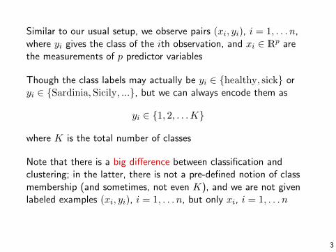
Binary classification and linear regression

Let’s start off by supposing that K = 2, so that the response isyi ∈ {1, 2}, for i = 1, . . . n

You already know a tool that you could potentially use in this casefor classification: linear regression. Simply treat the response as ifit were continuous, and find the linear regression coefficients of theresponse vector y ∈ Rn onto the predictors, i.e.,

β̂0, β̂ = argminβ0∈R, β∈Rp

n∑i=1

(yi − β0 − xTi β)2

Then, given a new input x0 ∈ Rp, we predict the class to be

f̂LS(x0) =

{1 if β̂0 + xT0 β̂ ≤ 1.5

2 if β̂0 + xT0 β̂ > 1.5

5

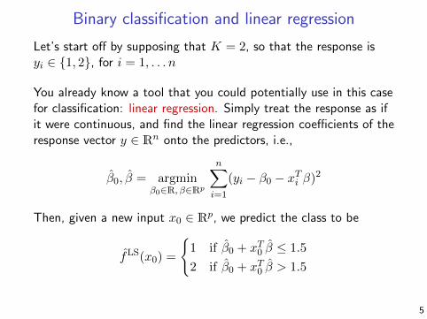
(Note: since we included an intercept term in the regression, itdoesn’t matter whether we code the class labels as {1, 2} or {0, 1},etc.)

In many instances, this actually works reasonably well. Examples:

●● ● ● ●● ●●●●● ●● ●● ●● ● ●● ● ●● ●●

● ●● ● ●● ● ●●● ●● ●● ●● ●● ●●● ●● ● ●

0.0 0.2 0.4 0.6 0.8

1.0

1.2

1.4

1.6

1.8

2.0

0 mistakes

x

y

●● ● ● ●● ●●●●● ●● ●● ●● ● ●● ● ●● ●●

● ●● ● ●● ● ●●● ●● ●● ●● ●● ●●● ●● ● ●

0.0 0.2 0.4 0.6 0.8

1.0

1.2

1.4

1.6

1.8

2.0

3 mistakes

x

y

●● ● ● ●● ●●●●● ●● ●● ●● ● ●● ● ●● ●●

●●● ● ●● ●●●● ●● ●● ●● ●● ●●● ●● ● ●

0.0 0.5 1.0 1.5

1.0

1.2

1.4

1.6

1.8

2.0

21 mistakes

x

y

Overall, using linear regression in this way for binary classification isnot a crazy idea. But how about if there are more than 2 classes?

6

Linear regression of indicators

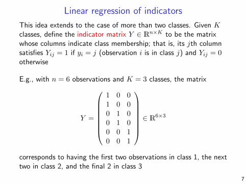
This idea extends to the case of more than two classes. Given Kclasses, define the indicator matrix Y ∈ Rn×K to be the matrixwhose columns indicate class membership; that is, its jth columnsatisfies Yij = 1 if yi = j (observation i is in class j) and Yij = 0otherwise

E.g., with n = 6 observations and K = 3 classes, the matrix

Y =

1 0 01 0 00 1 00 1 00 0 10 0 1

∈ R6×3

corresponds to having the first two observations in class 1, the nexttwo in class 2, and the final 2 in class 3

7

To construct a prediction rule, we regress each column Yj ∈ Rn(indicating the jth class versus all else) onto the predictors:

β̂j,0, β̂j = argminβj,0∈R, βj∈Rp

n∑i=1

(Yij − β0,j − βTj xi)2

Now, given a new input x0 ∈ Rp, we compute

β̂0,j + xT0 β̂j , j = 1, . . .K

take predict the class j that corresponds to the highest score. I.e.,we let each of the K linear models make its own prediction, andthen we take the strongest. Formally,

f̂LS(x0) = argmaxj=1,...K

β̂0,j + xT0 β̂j

8

The decision boundary between any two classes j, k are the valuesof x ∈ Rp for which

β̂0,j + xT β̂j = β̂0,k + xT β̂k

i.e., β̂0,j − β̂0,k + (β̂j − β̂k)Tx = 0

This defines a (p−1)-dimensionalaffine subspace in Rp. To oneside, we would always predict classj over k; to the other, we wouldalways predict class k over j

For K classes total, there are(K2

)= K(K−1)

2 decision boundaries

9

Ideal resultWhat we’d like to see when we use linear regression for a 3-wayclassification (from ESL page 105):

The plotted lines are the decision boundaries between classes 1 and2, and 2 and 3 (the decision boundary between classes 1 and 3never matters)

10

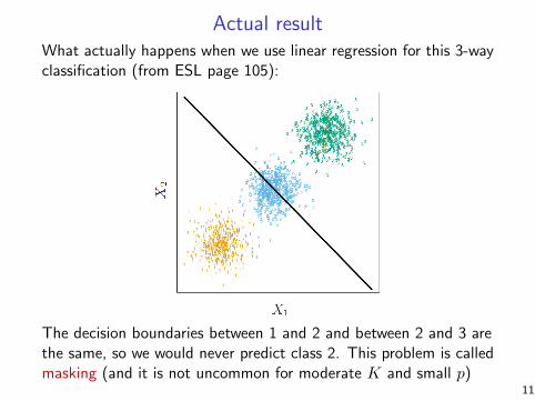
Actual resultWhat actually happens when we use linear regression for this 3-wayclassification (from ESL page 105):

The decision boundaries between 1 and 2 and between 2 and 3 arethe same, so we would never predict class 2. This problem is calledmasking (and it is not uncommon for moderate K and small p)

11

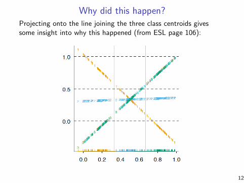
Why did this happen?Projecting onto the line joining the three class centroids givessome insight into why this happened (from ESL page 106):

12

Statistical decision theory

Let C be a random variable giving the class label of an observationin our data set. A natural rule would be to classify according to

f(x) = argmaxj=1,...K

P(C = j|X = x)

This predicts the most likely class, given the feature measurementsX = x ∈ Rp. This is called the Bayes classifier, and it is the bestthat we can do (think of overlapping classes)

Note that we can use Bayes’ rule to write

P(C = j|X = x) =P(X = x|C = j) · P(C = j)

P(X = x)

Let πj = P(C = j) be the prior probability of class j. Since theBayes classifier compares the above quantity across j = 1, . . .Kfor X = x, the denominator is always the same, hence

f(x) = argmaxj=1,...K

P(X = x|C = j) · πj

13

Linear discriminant analysis

Using the Bayes classifier is not realistic as it requires knowing theclass conditional densities P(X = x|C = j) and prior probabilitiesπj . But if estimate these quantities, then we can follow the idea

Linear discriminant analysis (LDA) does this by assuming that thedata within each class are normally distributed:

hj(x) = P(X = x|C = j) = N(µj ,Σ) density

We allow each class to have its own mean µj ∈ Rp, but we assumea common covariance matrix Σ ∈ Rp×p. Hence

hj(x) =1

(2π)p/2det(Σ)1/2exp

{− 1

2(x− µj)TΣ−1(x− µj)

}So we want to find j so that P(C = j|X = x) · πj = hj(x) · πj isthe largest

14

Since log(·) is a monotone function, we can consider maximizinglog(hj(x)πj) over j = 1, . . .K. We can define the rule:

fLDA(x) = argmaxj=1,...K

= argmaxj=1,...K

= argmaxj=1,...K

= argmaxj=1,...K

δj(x)

We call δj(x), j = 1, . . .K the discriminant functions. Note

δj(x) = xTΣ−1µj −1

2µTj Σ−1µj + log πj

is just an affine function of x

15

In practice, given an input x ∈ Rp, can we just use the rule fLDA

on the previous slide? Not quite! What’s missing: we don’t knowπj , µj , and Σ. Therefore we estimate them based on the trainingdata xi ∈ Rp and yi ∈ {1, . . .K}, i = 1, . . . n, by:

I π̂j = nj/n, the proportion of observations in class jI µ̂j = 1

nj

∑yi=j

xi, the centroid of class j

I Σ̂ = 1n−K

∑Kj=1

∑yi=j

(xi − µ̂j)(xi − µ̂j)T , the pooled samplecovariance matrix

(Here nj is the number of points in class j)

This gives the estimated discriminant functions:

δ̂j(x) = xT Σ̂−1µ̂j −1

2µ̂Tj Σ̂−1µ̂j + log π̂j

and finally the linear discriminant analysis rule,

f̂LDA(x) = argmaxj=1,...K

δ̂j(x)

16

LDA decision boundaries

The estimated discriminant functions

δ̂j(x) = xT Σ̂−1µ̂j −1

2µ̂Tj Σ̂−1µ̂j + log π̂j

= aj + bTj x

are just affine functions of x. The decision boundary betweenclasses j, k is the set of all x ∈ Rp such that δ̂j(x) = δ̂k(x), i.e.,

aj + bTj x = ak + bTk x

This defines an affine subspacein x:

aj − ak + (bj − bk)Tx = 0

17

Example: LDA decision boundaries

Example of decision boundaries from LDA (from ESL page 109):

fLDA(x) f̂LDA(x)

Are the decision boundaries the same as the perpendicular bisectors(Voronoi boundaries) between the class centroids? (Why not?)

18

LDA computations, usages, extensions

The decision boundaries for LDA are useful for graphical purposes,but to classify a new point x0 ∈ Rp we don’t use them—we simplycompute δ̂j(x0) for each j = 1, . . .K

LDA performs quite well on a wide variety of data sets, even whenpitted against fancy alternative classification schemes. Though itassumes normality, its simplicity often works in its favor. (Why?Think of the bias-variance tradeoff)

Still, there are some useful extensions of LDA. E.g.,

I Quadratic discriminant analysis: using the same normalmodel, we now allow each class j to have its own covariancematrix Σj . This leads to quadratic decision boundaries

I Reduced-rank linear discriminant analysis: we essentiallyproject the data to a lower dimensional subspace beforeperforming LDA. We will study this next time

19

Example: olive oil dataExample: n = 572 olive oils, each made in one of three regions ofItaly. On each observation we have p = 8 features measuring thepercentage composition of 8 different fatty acids. (Data from theolives data set from the R package classifly)

From the lda function in the MASS package:

●

●

●

●●●

●

●

●

●

●●

● ●

●

●

●

●

●

●●●

●

●

●

●

●

●

●●●

●

●●●●

●

●

●●

● ●●●

●

●●

●●

●

●●

●

●

●

●

●

●

●

●

●

●

●

●

●

●

●●

●●●● ●

●

●

●●

●

●

●●

●

●

●

●

●

●

●●

●●

●

●●

●

● ●

●

●

●

●

●

●

●●

●

●

●

●

●●

●

●

●

●

●●

●

●●

●

●

●

●●●●●

●

●●●

●

●

●●

●

●

●

● ●●

● ●

●

●

●

●

●●●

●

●

●●

●●

●●

●●

●

●

●

●●

●

●●

●

●

●●

●●

●

●

●●

●

●●

●

●

● ●

●

●

●

●

●●

●

●

●

●●

●

●● ●

●

●●

●

●●

● ●●

●

●

●●

●

●

●

●

●

●●

●

●●

●●

●

●

●

●

●

●

●●

●

●

● ●●

●

●●

●

●

●●

●

●

●

●

●

●

●

●

●

●

●

●

●

●

●

●

●●

●

●

●

●

●●

●

●●

●

●

●

●

●

●

●●

●

●

●●

●

●

●●

●●

●

●

●

●

●

●

●●

●

●

●●●

●

●●

●

●

●

●●

●

●●

●

●

●●

●

●

●

●

●●

●

● ●

●

●●

●●

●

●

●●●

●

●

●●

●

●

●●

●

●

●●

●

●

●●

●●

●

●

●

●●

●

●●

●

●

●

●

●

●

●

●

●

●

●

●

●●●●

●

●

●●●

●

●

●●

●

●

●

●●

●●

●●

●

●

●

●●

●

●●

●●

●●

●●

●

●●●

●

●

●●

●

●●●

●

●

●●

●

●

●

●●●

●●●

●

●

●

●

●

●●

●●

●

●●

●●●

●●

●

●●

●●

●

●

●●

●

●

●●

●

●

●

●

●

●

●

●●

●

●

●

●

●

●●

●

●●

●

●●●

●●

●

●

●

●

●● ●

●

●

●

●●

●

●

●

●

●

●

●

●

●

●

●● ●

●

●

●●

●●●

●

●

●

●

●●● ●

●

●

●●

●

●●●

●

●

●●

●

●

●

●

●●

●

●

●●●

●

●

●

● ●

●●

●●

●

●●

●

●

●

● ●

−18 −16 −14 −12 −10 −8

5254

5658

6062

LD1

LD2

This looks nice (seems that the observations are separated intoclasses), but what exactly is being shown? More next time...

20

Recap: linear regression of indicators, linear discriminantanalysis

In this lecture, we introduced the task of classification, a predictionproblem in which the outcome is categorical

We can perform classification for any total number of classes K bysimply performing K separate linear regressions on the appropriateindicator vectors of class membership. However, there can beproblems with this—when K > 2, a common problem is masking,in which one class is never predicted at all

Linear discriminant analysis also draws linear decision boundariesbut in a smarter way. Statistical decision theory tells us that wereally only need to know the class conditional densities and theprior class probabilities in order to perform classification. Lineardiscriminant analysis assumes normality of the data within eachclass, and assumes a common covariance matrix; it then replacesall unknown quantities by their sample estimates

21

Next time: more linear discriminant analysis; logisticregression

Logistic regression is a natural extension of the ideas behind linearregression and linear discriminant analysis.

●● ● ● ●● ● ●●●● ●● ●● ●● ● ●● ● ●● ●●

● ●● ● ●● ● ●●● ●● ●● ●● ●● ●●● ●● ● ●

0.0 0.2 0.4 0.6 0.8

0.0

0.2

0.4

0.6

0.8

1.0

x

y

22