This paper presents preliminary findings and is being distributed to economists

and other interested readers solely to stimulate discussion and elicit comments.

The views expressed in this paper are those of the authors and are not necessarily

reflective of views at the Federal Reserve Bank of New York or the Federal

Reserve System. Any errors or omissions are the responsibility of the authors.

Federal Reserve Bank of New York

Staff Reports

The Capital and Loss Assessment under Stress

Scenarios (CLASS) Model

Beverly Hirtle

Anna Kovner

James Vickery

Meru Bhanot

Staff Report No. 663

February 2014

The Capital and Loss Assessment under Stress Scenarios (CLASS) Model

Beverly Hirtle, Anna Kovner, James Vickery, and Meru Bhanot

Federal Reserve Bank of New York Staff Reports, no. 663

February 2014

JEL classification: G21, G17, G01

Abstract

The CLASS model is a top‐down capital stress testing framework that projects the effect of

different macroeconomic scenarios on U.S. banking firms. The model is based on simple

econometric models estimated using public data and also on assumptions about loan loss

provisioning, taxes, asset growth, and other factors. We use this framework to calculate a

projected industry capital gap relative to a target ratio at different points in time under a common

stressful macroeconomic scenario. This estimated capital gap began rising four years before the

financial crisis and peaked at the end of 2008. The gap has since fallen sharply and is now

significantly below precrisis levels. In the cross-section, firms projected to be most sensitive to

macroeconomic conditions have higher capital ratios, consistent with a “precautionary” view of

bank capital.

Key words: capital, stress testing

_________________

Bhanot, Hirtle, Kovner, Vickery: Federal Reserve Bank of New York (e-mail:

meru.bhanot@ny.frb.org, beverly.hirtle@ny.frb.org, anna.kovner@ny.frb.org,

james.vickery@ny.frb.org). The authors thank Dafna Avraham, Peter Hull, Lev Menand, and Lily

Zhou for outstanding research assistance, as well as many Federal Reserve colleagues for their

suggestions and ideas. The views expressed in this paper are those of the authors and do not

necessarily reflect the position of the Federal Reserve Bank of New York or the Federal Reserve

System.

 

1  

1. Introduction 

Central banks and bank supervisors have increasingly relied on capital stress testing as a supervisory 

and macroprudential tool. The recent financial crisis highlighted the importance of the amount and 

quality of capital at large banking companies in ensuring public confidence in individual financial 

institutions and in the financial system as a whole. Stress tests have been used by central banks and 

supervisors to assess the resilience of individual banking companies to adverse macroeconomic and 

financial market conditions, as a way of gauging additional capital needs at individual firms, and as 

means of assessing the overall capital strength of the banking system. In the United States, the first 

formal supervisory stress tests – the Supervisory Capital Assessment Program (SCAP) – were 

performed during 2009, and stress tests have since become a permanent supervisory and 

macroprudential tool through the implementation of the stress test provisions of the Dodd‐Frank 

Act (Dodd‐Frank Act Stress Tests, or DFAST) and the Comprehensive Capital Analysis and Review 

(CCAR)1. Bank supervisors in Europe conducted coordinated stress tests of the largest European 

banking companies in 2010 and 2011.2 A number of central banks have also constructed system‐

wide stress test frameworks to assess the robustness of their banking systems to adverse 

macroeconomic environments and stressed funding conditions.3 

 

In this paper, we describe a framework for assessing the impact of macroeconomic conditions on 

the capital and performance of the U.S. banking system – the Capital and Loss Assessment under 

Stress Scenarios (CLASS) model. The CLASS model is a “top‐down” model of the U.S. commercial 

banking industry that generates projections of commercial bank and bank holding company (BHC) 

income and capital under different macroeconomic scenarios. These projections are based on a set 

of 22 regression models of components of bank income, expense and loan performance, combined 

with assumptions about provisioning, dividends, asset growth and other factors. Similar to models 

produced by some other central banks, the goal of the CLASS model is to produce system‐wide 

estimates and distributions of net income and capital. To do this, the model first generates 

                                                       1See Board of Governors of the Federal Reserve System (2009a, 2009b, 2012, 2013a, 2013b) for more detail on the SCAP, CCAR and DFAST stress tests. Bookstaber et al. (2013) and Greenlaw et al. (2012) discuss use of supervisory stress tests for macroprudential purposes. 2 See Committee of European Banking Supervisors (2010) and European Banking Authority (2011) for details and results of the European stress tests. 3 For instance, Kapadia et al. (2012) describe the RAMSI model developed by the Bank of England and Wong and Hui (2009) describe a model developed at the Hong Kong Monetary Authority to assess liquidity risk. 

 

2  

projections for each of the 200 largest domestic banking institutions, as well as the aggregated 

remainder of the industry. These projections are then summed to create industry projections or 

distributions of outcomes across firms.  

 

Projections from the CLASS model provide insight into the capital resiliency of the U.S. banking 

system against severely stressed economic and financial market conditions. These projections 

suggest that the U.S. banking industry’s vulnerability to undercapitalization has declined, not only 

relative to the financial crisis of 2007‐09, but also relative to the period preceding the crisis. CLASS 

model projections indicate an increasing capital “gap” (a shortfall of capital under stressed 

economic conditions) starting in 2004, well before deterioration in market‐based measures of 

capital adequacy.  

 

Looking cross‐sectionally, CLASS model projections based on current industry data suggest that 

firms projected to experience large declines in capital under stressful economic conditions also tend 

to have higher current capital ratios. This relationship is consistent with a “precautionary” view of 

bank capital; that is, banks engaged in risky activities also hold a higher capital buffer to limit the 

likelihood of financial distress. We find no robust relationship between projected declines in capital 

ratios under stress and banking institution size or the fraction of liquid assets. 

 

The CLASS model’s top‐down approach is intended to complement more detailed supervisory 

models of components of bank revenues and expenses, such as those used in the DFAST, CCAR and 

European stress tests. Unlike such models, the CLASS model relies only on public information, 

namely macroeconomic and financial market data combined with bank and BHC regulatory report 

filings. The use of regulatory report data allows us to compute projections easily for a much larger 

number of firms and with greater frequency than is practical from detailed bottom‐up analysis using 

supervisory data collected directly from BHCs. In addition, the CLASS framework is relatively simple 

to understand, and can produce quarterly income and capital projections quickly (in only a couple 

of minutes for a single macroeconomic scenario). Thus it can, for example, be used for simulations 

or to provide immediate back‐of‐the envelope estimates of the effect of a particular 

macroeconomic shock on the U.S. banking system.  

 

 

3  

Balanced against these advantages, the CLASS model’s “top‐down” approach also has some 

significant limitations. For example, it abstracts from many idiosyncratic differences between 

individual institutions. For this reason, while the model can reasonably be used to model aggregate 

net income and capital, and the overall distribution of capital across institutions, caution should be 

exercised in using the model to project the capital of a specific bank or BHC. In addition, the model 

also does not, at least at the present time, incorporate any feedback from the banking system to 

the macroeconomy or to financial markets. Instead, the macroeconomic projections used as inputs 

to the model are essentially treated as exogenous. This paper presents a series of results illustrating 

the sensitivity of the CLASS model outcomes to certain key assumptions, such as balance sheet 

growth, dividend behavior, and the level of the allowance for loan and lease losses. These results 

are pertinent not just for the CLASS model, but have more general implications for other stress test 

frameworks that incorporate assumptions about these same factors.  

 

The rest of this paper describes the CLASS model in more detail, focusing on a macroeconomic 

scenario that repeats the economic conditions realized in the recent financial crisis. Section 2 

details the framework and analytical approach. Section 3 presents examples of the kind of output 

the model can produce, including projections of aggregate net income and post‐stress capital ratios 

for the U.S. banking system under a range of hypothetical adverse scenarios, focusing on how 

different elements and assumptions of the CLASS model affect these projections. Section 4 reviews 

the model’s sensitivity to different assumptions and Section 5 concludes. 

  

2. Details of the CLASS Model 

A. Framework and Analytical Approach 

The CLASS model is designed to project net income and capital for individual banks and BHCs over a 

future period of two to three years (the “stress test horizon”) under different macroeconomic and 

financial market scenarios. The macroeconomic scenarios are defined by a set of economic and 

financial market variables – such as GDP growth, the unemployment rate, housing prices, equity 

prices, short‐term and long‐term interest rates, and credit spreads – that are likely to influence the 

profitability of banking institutions. The key outputs of the CLASS model are projections of net 

income and capital given assumed paths for these economic and financial market variables over the 

stress test horizon. 

 

4  

 

Figure 1 presents an overview of the CLASS model’s structure and the main steps involved in 

generating projections of net income and capital. The core of the CLASS model is a series of 

regression equations that model how various financial ratios (e.g. the net interest margin (NIM), net 

chargeoff rates on different types of loans) evolve over time, given macroeconomic conditions, the 

lagged value of the financial ratio, and other controls. The regression equations dynamically 

generate forecasts of these ratios for each banking firm over the stress test horizon, using the 

macroeconomic scenario variables and current financial data for the firm as inputs. These ratio 

projections are converted to dollar values by multiplying by loan balances (in the case of loan loss 

rates), securities balances (in the case of securities losses), or assets (in the case of revenue and 

expense items). Taken together, the loss, revenue, and expense projections, combined with 

auxiliary assumptions, generate a projection of pre‐tax net income for each BHC and bank. Changes 

in regulatory capital and regulatory capital ratios are derived by combining these pre‐tax net 

income projections with assumptions about dividends, the impact of taxes, and regulatory capital 

rules, along with assumptions about growth of risk‐weighted assets (RWA). Projections for each 

firm are then summed up to generate systemwide results. 

 

Figure 2 presents a more detailed schematic of the CLASS model structure. The first key component 

of projected net income is pre‐provision net revenue (PPNR), an accounting measure defined as net 

interest income (interest income earned minus interest expense) plus non‐interest income 

(including trading income, as well as nontrading noninterest income earned from fees and other 

sources), minus non‐interest expense (compensation, expenses related to premises and fixed 

assets, and other non‐credit‐related expenses). The CLASS model includes six equations for financial 

ratios reflecting different components of PPNR. The dollar PPNR projection is computed as the 

product of each projected ratio by the balance of the relevant denominator (e.g. trading income is 

the product of the return on trading assets and the trading asset balance) for each firm and quarter 

over the forecast horizon.  

 

The next net income component is provision expense for loan and lease losses. We first compute 

projected net chargeoffs (NCOs) based on NCO rates on 15 different categories of loans. CLASS 

 

5  

includes a rule that then translates current net chargeoffs and the level of loan loss reserves into 

provision expense. This provisioning rule is described in more detail below.  

 

Pre‐tax net income equals PPNR minus provision expense for loan losses plus projected gains or 

losses on investment securities held in the firm’s available‐for‐sale (AFS) and held‐to‐maturity 

(HTM) portfolios. The model includes an econometric model for AFS returns. Returns on HTM 

portfolios, which are generally small for most firms, are assumed to be zero. After‐tax net income is 

calculated using a constant, assumed tax rate applied to all banks and BHCs. CLASS allows firms to 

accumulate deferred tax assets (DTAs) as a result of pre‐tax losses incurred. However, since US 

financial regulation limits the extent to which these DTAs can be recognized for regulatory capital 

purposes, CLASS includes an adjustment to recognize these limits, discussed below.  

 

CLASS then computes the evolution of capital for the firm, based on the path of net income 

combined with a behavioral rule for dividends and other distributions. Note that the CLASS model 

projects net income and regulatory capital ratios as they would occur over time under the particular 

macroeconomic scenario, rather than generating estimates of marked‐to‐market values of the 

banks’ assets or capital or estimating the impact of an instantaneous roll‐forward of peak‐to‐trough 

scenario conditions. As such, the CLASS model projections follow U.S. generally accepted 

accounting principles (GAAP) and U.S. regulatory capital rules. In particular, loss and revenue 

projections reflect the U.S. GAAP treatment of the underlying positions. Trading revenue (part of 

non‐interest income) is based on marked‐to‐market changes in trading account assets plus fees and 

spreads earned on trading activities; loan losses are based on projected provisions into the 

allowance for loan and lease losses (ALLL), which are in turn derived from projected loan charge‐

offs; and projected investment securities gains and losses incorporate the combination of realized 

gains and losses from sales and other than temporary impairment (OTTI) of securities in the AFS and 

HTM portfolios.  

 

Regulatory capital ratios are calculated using current U.S. regulatory capital rules, including the 

definitions of regulatory capital and rules for calculating risk‐weighted assets. In this regard, the 

 

6  

current version of the CLASS model primarily reflects Basel 1 risk weights4, since these are the rules 

under which U.S. banks and BHCs currently calculate their regulatory capital ratios. As banks and 

BHCs transition from Basel 1 to Basel 2 risk‐weights and eventually the new Basel 3 regulatory 

capital definitions over time, the CLASS model will incorporate these changes into the projections. 

Following practice in the DFAST and CCAR stress tests, the primary capital metric in the CLASS 

model projections is Tier 1 common equity, defined as common equity minus the deductions from 

Tier 1 capital (such as certain intangible assets) required under U.S. regulatory capital rules.  

 

B. Comparing CLASS to DFAST & CCAR 

A natural point of comparison for the CLASS model is the framework used in the Federal Reserve’s 

DFAST and CCAR stress tests. At a conceptual level, the analytical approach in both sets of stress 

test calculations is the same: to project net income and post‐stress regulatory capital ratios as they 

would occur, quarter‐by‐quarter, over the stress test scenario horizon, applying U.S. accounting and 

regulatory capital rules. However, there are important differences in implementation that affect the 

comparability of the results, as summarized in Table 1. 

 

To begin, the modeling approach used in CLASS is much more aggregated than the Federal 

Reserve’s stress tests. For the most part, the DFAST and CCAR stress test results are derived from 

detailed “bottom up” models based on granular risk characteristics of the loan, securities, and 

trading portfolios, often at the individual borrower, loan or position level. These models use 

detailed data provided by the BHCs describing borrower characteristics, loan or securities structure, 

and other factors likely to affect the default probability, exposure at default, and loss given default 

of the positions. In contrast, the CLASS model uses a “top down” modeling approach based on the 

historical behavior of charge‐offs, securities gains and losses, trading performance, and other 

revenue and expense variables. While the input data for these models are firm specific, regulatory 

report data, the information is less granular and detailed than the BHC‐specific data used in the 

CCAR and DFAST stress tests. 

 

                                                       4 An important exception is trading‐related risk‐weighted assets at the largest BHCs, which are calculated under “Basel 2.5” rules starting with the first quarter of 2013 and for all subsequent quarters. These rules significantly increase trading‐related risk‐weighted assets at these firms. 

 

7  

Reflecting the modeling approach in the CLASS model, the focus of the results is on the industry as a 

whole, or the overall distribution of results, rather than projections for individual BHCs. Industry‐

level results are generated by producing results for the 200 largest commercial banking firms (BHCs 

and independent banks) and aggregating the remaining institutions into a single 201st proxy BHC. In 

contrast, the most recent DFAST and CCAR stress tests were performed on 18 individual large BHCs 

and results are reported in both the aggregate for these firms and at the individual BHC level. 

Starting in 2014, the set of BHCs in the DFAST and CCAR stress tests will expand to include another 

approximately dozen BHCs with assets greater than $50 billion. 

 

There are also differences in some of the detailed modeling elements that affect both the nature of 

the loss projections and magnitude of the resulting post‐stress capital ratios.  

Trading and counterparty losses: the DFAST and CCAR stress tests include an instantaneous 

global market shock on trading and counterparty positions at the six largest BHCs, which is 

assumed to occur in the first quarter of the stress test horizon. The CLASS model does not 

include this trading shock specifically, though the trading revenue model is geared to 

produce the kind of large trading losses that were experienced during the recent financial 

crisis if the macroeconomic scenario contains financial market conditions similar to those 

experienced during the crisis. Even so, the additional global market shock included in the 

DFAST and CCAR stress tests is likely to generate larger trading and counterparty losses at 

the largest BHCs than the CLASS model.  

Balance sheets: the CLASS model includes stylized assumptions about balance sheet growth 

that do not vary across BHCs or across macroeconomic scenarios. In contrast, the CCAR and 

DFAST stress tests include balance sheet growth paths that vary across both these 

dimensions. As illustrated later in this paper, differences in balance sheet growth can have 

significant impacts on the resulting projections of post‐stress capital ratios, largely due to 

the impact on projected RWA, the denominator of those ratios.  

Dividend and capital distribution assumptions: The CLASS model makes stylized assumptions 

about common stock dividends – linking these to earnings and an assumed long‐run payout 

ratio – and repurchases. This means that the dividends in the CLASS model are sensitive to 

individual BHC performance and will change with the macroeconomic scenario; generally, 

dividends will be higher in good economic environments than in the stressed ones. The 

 

8  

DFAST stress test results also make stylized assumptions about dividends, assuming that 

they are fixed at recent historical levels. Thus, dividends do not vary across or within 

macroeconomic scenarios in the DFAST stress tests.  

Regulatory Capital Rules:The CCAR and DFAST stress tests incorporate RWA projections that 

capture the phase‐in of any new capital regulations over the stress test horizon. In contrast, 

the CLASS model RWA projections implicitly carry forward the regulatory capital rules in 

place at the time of the last historical observation, since RWAs are assumed to grow 

proportionately with assets.  

 

C. Regression equation structure 

Each CLASS regression equation models a key income or expense ratio as a function of an 

autoregressive (AR(1)) term and a parsimonious set of macroeconomic variables. Some equations 

are estimated as time‐series models using historical data summed up across all BHCs and banks. 

Other models are estimated using pooled quarterly data on individual firms, allowing us to control 

for firm characteristics such as the composition of assets. 

 

The time series specifications take the general form: 

ratiot = α + β1 ratiot‐1 + β2 macrot + εt 

 

where ratiot is the financial ratio of interest and ratiot‐1 is an AR(1) term, macrot is the set of 

macroeconomic variables appropriate to that ratio. When statistically and economically significant, 

we also include a linear time trend in the specification. The specification of each equation – in 

particular, the macroeconomic variables included and the form of those variables – was determined 

by assessing statistical significance, judging whether the sign and size of the coefficients were 

economically reasonable and consistent with economic theory, and through evaluating in‐sample 

and out‐of‐sample projection performance.  

 

For the models estimated using pooled individual BHC and bank data, we instead estimate the 

specification: 

ratiot,i = α + β1 ratiot‐1,i + β2 macrot,i + β3 Xt,i + εt , 

 

 

9  

where each observation is now indexed by firm i, and we include Xt,i , a vector of firm‐specific 

characteristics, such as shares of different types of loans in the loan portfolio5 or the share of risky 

securities in the investment securities portfolio. We estimate pooled regressions for the AFS returns 

equation, and for components of PPNR significantly affected by the composition lending activities 

or business line focus, such as net interest margin, compensation expense, and other non‐interest 

expense. 

 

The autoregressive nature of each equation implies that the projected ratio for each firm will 

converge slowly from its most recent historical value towards a long‐run steady state value. These 

paths will be significantly influenced by the assumed macroeconomic scenario. The autoregressive 

structure also means that the CLASS model projections are sensitive to the first‐lagged value of the 

bank and BHC data that are used to “seed” the model projections. The seed data is particularly 

important for income and expense categories that are estimated to be highly autoregressive (that 

is, with a large value of β1); in such categories, a low or high ratio value in the historical quarter 

used to seed the model will have persistent effects on the projected income path over the forecast 

horizon.6 On occasion, the autoregressive structure of the CLASS regression equations can create 

unrealistic shifts in projected income and capital in cases when an individual BHC or bank 

experiences an idiosyncratically large income spike that may be unlikely to be repeated in future 

quarters (e.g. realization of a large loss related to a legacy acquisition). In such cases, we apply a 

correction to the model projections so that the shock in question does not have a persistent effect 

on projected income. In practice, we make such judgmental adjustments to the model projections 

only relatively rarely. 

 

D. Data 

                                                       5 For example, the net interest margin (NIM) equation includes controls for the composition of the firm’s loan portfolio. This is necessary because interest margins vary significantly across firms (e.g. margins are higher for firms with a high concentration of credit card loans, due to the high interest rates on credit card facilities). This implies that even the long‐run NIM projection will vary across firms, reflecting differences in these portfolio shares. 6 On the whole, this persistence is realistic, given the historical dynamics of bank income, and given that our 

regression models are estimated to maximize fit to the historical data. 

 

10  

To estimate the equations described above we combine two types of data measured at a quarterly 

frequency: regulatory report data on balance sheets, income and loan performance, and 

macroeconomic and financial market data used in the macroeconomic scenarios.  

 

The BHC and bank regulatory data are drawn from Federal Reserve Y‐9C regulatory filings for BHCs 

and FFIEC Consolidated Reports of Condition and Income (Call Report) filings for commercial banks. 

The regressions are based on quarterly data from 1991 to the present for all BHCs that file the FR Y‐

9C, plus the subset of commercial banks that do not have a parent that files a FR Y‐9C.7 The data 

include all U.S.‐headquartered, top‐tier BHCs and independent commercial banks, as well as six large 

foreign‐owned BHCs subject to CCAR in 2014. Other BHCs and commercial banks whose parent is 

domiciled outside the United States are excluded, as are two BHCs that are not engaged in traditional 

commercial banking activities: DTCC and ICE Holdings.  

 

As noted above, the majority of the regression specifications are based on an aggregated time 

series for the banking system, calculated by summing data across the individual banking firms. 

These aggregate series are subject to breaks when new institutions become banks or BHCs or when 

a BHC makes a significant acquisition from outside the banking industry. For example, in the first 

quarter of 2009, the conversion of Goldman Sachs, Morgan Stanley, and other large financial firms 

to a bank holding company charter led to a significant increase in total industry assets. Similarly, 

acquisitions of non‐bank financial firms, such as JPMorgan Chase’s acquisition of Washington 

Mutual and Bear Stearns, and Bank of America’s acquisition of Merrill Lynch, also create 

discontinuities. We do not make any adjustments for these breaks, in part because the pre‐

conversion or pre‐acquisition data on the target firm needed to make such adjustments are not 

readily available in a format comparable with the Call and Y‐9C reports. However, since the 

regression variables are specified as ratios – and the newly converted or acquired institution enters 

both the numerator and denominator of the ratio – the impact of these breaks is somewhat muted. 

 

For the regression specifications based on a pooled sample of firms rather than aggregate industry 

data, we create a panel of the 200 largest banking institutions by assets in each specific quarter. The 

                                                       7 This includes both commercial banks that are self‐held and commercial banks that have holding companies that are too small to file a consolidated regulatory Y‐9C filing.  

 

11  

remaining banks and BHCs are aggregated into a single observation, resulting in a total sample of 

201 entities. 

 

The regression equations include parsimonious combinations of nine macroeconomic and financial 

market variables summarizing economic activity and financial market conditions. The variables are a 

subset of those included in the scenarios provided by the Federal Reserve for the DFAST stress 

tests, and include the 10‐year Treasury bond yield, the 3‐month Treasury bill yield, the civilian 

unemployment rate, real gross domestic product (GDP), the CoreLogic U.S. home price index, the 

BBB bond index yield, commercial real estate prices and the U.S. Dow Jones Total Stock Market 

Index. Table 2 provides a full list of macroeconomic and financial market variables included in the 

CLASS model equations and describes the transformation of each variable used in the regressions 

(e.g. that is, whether the variable is expressed in levels, changes, percent changes, or some other 

form). 

 

E. Regression model estimates 

The CLASS model includes six regression equations for components of PPNR, fifteen equations for 

net charge‐off (NCO) rates on different loan categories (e.g. first‐lien residential real estate, 

construction loans, credit cards, C&I loans), and an equation for gains and losses on the AFS 

securities portfolio. Table 3 presents summary statistics for these twenty‐two ratios that are 

projected as part of the CLASS framework. Table 4 summarizes the set of macroeconomic variables 

included in each equation, and indicates which are statistically significant. Detailed equation 

specifications and parameter estimates are presented in Appendix A. 

 

i. PPNR 

We separately model net interest income (that is, interest income minus interest expense), trading 

income (which includes both mark‐to‐market changes in value of trading positions and derivatives 

as well as fee and spread income on trading activities), non‐interest non‐trading income (such as 

deposit fees, income from fiduciary activities, and revenues from investment banking and 

insurance), and three components of noninterest expense: compensation expense, expenses 

 

12  

related to premises and fixed assets, and other non‐interest expense.8 Each of these components of 

PPNR is expressed as a ratio either of total assets (for non‐interest, non‐trading income, 

compensation expense, fixed asset expense, and other non‐interest expense), trading assets (for 

trading revenue), or interest‐earning assets (for net interest income). 

 

Each PPNR equation except for return on trading assets is estimated by weighted least squares 

using the pooled regression approach, weighting by the institution’s share of the relevant 

denominator asset balance (e.g. interest‐earning asset share in the case of net interest margin). 

Pooled regressions include controls for the composition of firm assets and firm size: namely the 

ratio of residential real estate loans, commercial real estate loans, commercial and industrial loans, 

credit card loans, trading assets, and securities to interest earning assets, and the firm’s assets 

scaled by industry assets in the quarter.  

 

Given the inclusion of these controls, the projected PPNR ratio for each BHC or bank converges to 

the long‐run conditional mean for firms with similar business focus and size, rather than the 

unconditional sample mean. These controls are particularly important for the net interest margin 

equation, since the spread between borrowing and lending rates varies significantly across types of 

loans. For example, credit card balances historically have high net interest margins, compensating 

for the higher credit risk associated with these loans.  

 

In our final specifications, the net interest margin is positively related to the slope of the yield curve, 

trading returns are sensitive to credit spreads (the change in the yield spread between BBB‐rated 

and AAA‐rated corporate bonds), and nontrading noninterest income is sensitive to stock returns. 

Compensation expense is positively correlated with stock returns, while other noninterest expense 

is sensitive to credit spreads. As shown in the detailed results presented in appendix A, most 

components of PPNR are highly autoregressive, with the exception of the return on trading assets. 

As noted above, trading revenue is a combination of ongoing revenue earned from intermediating 

trading‐related activities (e.g., market‐making) and any mark‐to‐market trading gains or losses. 

These mark‐to‐market earnings fluctuate with returns on the underlying asset classes held by the 

                                                       8 As part of the CLASS model development work, we estimated similar models for aggregate PPNR. Explanatory power and sensitivity to macroeconomic conditions are lower for the aggregate model.  

 

13  

firm, although given the complexity of the trading positions held by firms, the relationship between 

a given macroeconomic variable and mark‐to‐market trading losses is likely to vary significantly 

across firms and through time. 

 

ii. Loan Net Charge‐Off Rates 

The CLASS model includes 15 NCO models for major loan categories: first lien and junior lien 

residential mortgages, home equity lines of credit (HELOC), construction loans, multifamily and non‐

farm non‐residential commercial mortgages, credit cards, other consumer loans, commercial and 

industrial (C&I) loans, leases, loans to foreign governments, loans to depository institutions, 

agriculture loans, other real estate loans, and all other loans. In each case, dollar net charge‐offs are 

scaled by the corresponding loan balance, so that the regression dependent variables is a loss rate. 

 

NCO rates on real estate loans are primarily associated with property price downturns. From a 

theoretical perspective, mortgage default represents a put option on the underlying real estate 

used to collateralize the loan (e.g., Kau et al, 1992). Consistent with this point, we find that the 

empirical relationship between real estate price growth and real‐estate loan charge‐offs is highly 

non‐linear, with real estate price declines having a much larger effect on charge‐off rates than real 

estate price increases. For this reason, the final equations include an interaction between property 

price growth and a dummy variable for whether the change in the price index is less than zero. 

Quantitatively, this interaction term is the key macroeconomic determinant of mortgage NCO rates 

in the models. Property price growth is measured as the year‐over‐year log change in either 

residential or commercial property prices. Conversely, mortgage chargeoffs are generally less 

closely associated with the broader state of the business cycle than other loan categories.9  

 

For non‐mortgage loans, we found that the change in the unemployment rate was generally the 

macroeconomic variable most correlated with loan losses, with an increase in the unemployment 

                                                       9 This is particularly true for residential mortgage charge‐offs, which were low and relatively insensitive to macroeconomic conditions until the recent financial crisis. Although commercial real estate charge‐offs were high in the early 1990s, NCOs in this category were also low between this episode and the recent crisis. We found that business cycle indicators such as the change in the unemployment rate were generally statistically insignificant once we controlled for real estate price growth; consequently these variables were not included in the final specifications. 

 

14  

rate causing charge‐off rates to increase. Quantitatively, credit card charge‐offs are particularly 

sensitive to changes in unemployment. Across the entire spectrum of loan categories, net charge‐

off rates are highly autoregressive, with AR(1) coefficients generally ranging between 0.5 and 0.9. 

 

iii.  Returns on Available‐for‐Sale (AFS) portfolios  

Realized gains and losses in a banking firm’s AFS securities portfolios occur only when the firm sells 

those assets or the securities are deemed to have experienced “Other Than Temporary 

Impairment” or OTTI. Under current GAAP accounting, OTTI status is determined only by credit 

factors, and need not incorporate changes in market prices due to interest rate risk, liquidity or 

other factors, until the bonds are sold. Realized AFS gains and losses thus reflect a combination of 

asset price shocks, credit events, behavioral decisions about asset sales, and accounting judgment. 

Historically, AFS returns are typically low and stable, but with idiosyncratic large downward 

movements, particularly during 2008 and 2009. 

 

Our approach to modeling AFS securities recognizes the significant variation in the riskiness of these 

portfolios across firms and through time. In the spirit of the approach used in the DFAST and CCAR 

stress tests, the CLASS model categorizes AFS securities backed by the U.S. government or 

government agencies as “safe” assets that are unlikely to experience credit impairment and thus 

incur OTTI. All other AFS securities are classified as “risky,” including municipal bonds, non‐agency 

mortgage‐backed securities and asset‐backed securities, and corporate debt.10 Realized gains and 

losses on risky securities should be more sensitive to credit spreads. Consistent with this view, we 

find that an interaction term between the share of AFS securities that are risky and increases in the 

credit spread (BBB minus AAA) is a key driver of AFS securities returns. This interaction term 

captures variation in the composition of AFS portfolios both across institutions and through time – 

an important consideration given that the aggregate fraction of AFS securities consisting of risky 

assets increased from less than 30 percent in 1994 to approximately half by 2010. AFS returns are 

also found to be negatively correlated with the change in Treasury bond yields. 

 

                                                       10 Prior to 2001, BHCs and banks only reported the breakdown of risky securities into: securities issued by states and municipalities, foreign and domestic equity and debt securities. U.S. government agency and corporation obligations were reported without separately breaking out MBS. 

 

15  

F. Asset and Liability Growth 

As discussed above, the 22 regression equations produce projections of accounting ratios – losses, 

revenues or expenses scaled by a loan, securities or asset balance. To translate these ratios into 

dollar values in order to calculate net income, the CLASS model requires projections of the balance 

sheet over the stress test horizon. Balance sheet projections are also needed to project risk‐

weighted assets and to calculate capital ratios, since these ratios have either risk‐weighted assets or 

total assets in the denominator. Because of this mechanical relation between capital ratios and 

asset balances, the results of CLASS and other stress testing models based on accounting data are 

significantly sensitive to the growth path of assets over the stress test horizon, as illustrated in the 

sensitivity exercise presented in section 4 of this paper. 

 

A key question, then, is what to assume about balance sheet growth and composition over the 

stress test horizon. Historical banking industry data illustrate that both the growth rate of bank 

assets as well as the composition of the balance sheet (that is, the proportion of assets held in 

different types of loans and securities and the share of deposits and other debt in liabilities) can 

vary significantly with economic conditions.11 Developing models to capture this cyclical variation, 

as well as firm‐specific strategic and business focus considerations, is a complex challenge.  

 

Currently, the CLASS model adopts a simple approach to balance sheet projections ‐‐ each BHC or 

bank’s total assets are assumed to grow at a fixed percentage rate of 1.25% per quarter (5% per 

year) over the stress test horizon. This growth rate was chosen to be roughly consistent with the 

long‐run nominal historical growth of assets in the U.S. banking industry in the period since 

disinflation. The same growth rate is assumed for all asset balances, implying that the composition 

of the balance sheet– that is, the proportion of total assets represented by different types of loans, 

securities, cash, trading positions, other assets – stays fixed at its last historical value over the stress 

test horizon. The composition of liabilities is also assumed to stay fixed, while the book value of 

liabilities is calculated so that the balance sheet identity (assets equal liabilities plus capital) holds at 

each point in time. 

 

                                                       11 For instance, Clark et al. (2007) documents the cyclical variability in the share of retail‐related loans such as mortgages and credit cards. 

 

16  

Assuming that growth rate of assets is the same for all institutions and for all scenarios is not 

“realistic” in the sense that banking industry assets historically tend to grow more slowly in stressed 

economic environments than they do during expansions. However, assuming that banking industry 

assets continue to grow during economic stress can be seen as rigorous from both microprudential 

and macroprudential perspectives. From a macroprudential perspective, it ensures that 

assessments of banking industry capital strength are made in the context of continued availability 

of credit12, while from a microprudential perspective, firm‐level capital projections are made under 

the assumption that the firm continues to function as an active financial intermediary. 

 

G. Allowance for Loan and Lease Losses 

The CLASS framework’s net charge‐off models, combined with assumptions about the evolution of 

loan balances, allow us to calculate total dollar net charge‐offs each quarter over the forecast 

horizon. However, as already noted, under U.S. accounting rules, net charge‐offs do not directly 

affect net income. Instead, accounting rules recognize the provision expense incurred to increase 

the reserve held against loan losses, known as the allowance for loan and lease losses (ALLL). In 

brief, under U.S. GAAP, banking firms establish the ALLL to account for losses on loans or loan 

portfolios that can reasonably be expected to have occurred but have not yet been written down 

via a charge‐off. There is a direct mathematical relationship between the ALLL, charge‐offs, and 

provision expense: 

 

ALLLt = ALLLt‐1 + Provision for loan and lease lossest – Net chargeoffst 

 

Given this identity, translating the CLASS model’s projections of net charge‐offs into provision 

expense is isomorphic to determining the appropriate level of the ALLL. This is not a straightforward 

exercise, however, since ALLL is not computed mechanically, but instead is estimated by the firm 

based on a set of accounting guidelines which leave scope for managerial discretion and judgment. 

Moreover, as an empirical matter, the choice of provisioning rule has a quantitatively important 

effect on net income and thus on the regulatory capital projections (see section 4).  

 

                                                       12 Greenlaw et al. (2012) argue in favor of this approach. 

 

17  

For interested readers, a detailed discussion of issues around loan loss provisioning is presented in 

appendix B. To summarize, in setting the provisioning rule, we draw on supervisory guidance about 

the ALLL which suggests that the ALLL should generally at minimum be sufficient to cover at least 

four quarters of recent charge‐offs (Office of the Comptroller of the Currency et al., 2006; Federal 

Reserve Board, 2013). In particular, the CLASS model assumes that the ALLL is bounded in a range 

relative to projected future net charge‐offs. If the ALLL is at least equal to the next four quarters of 

projected net charge‐offs (under the macro scenario in question) but not greater than 250% of that 

level, then provision expense in the quarter is set equal to current‐quarter net charge‐offs. If the 

ALLL is below four quarters of future charge‐offs, then provision expense is set equal to an amount 

that would bring the ALLL to that level (so provisions would exceed net charge‐offs for that 

quarter). However, if the ALLL is greater than twice four quarters of future net charge‐offs, then 

provision expense is negative (an ALLL release), to bring the ALLL down to that level.  

 

If necessary, we also adjust the ALLL at the start of the forecast horizon to ensure that the starting 

value of ALLL is inside this 100% to 250% range. To maintain the accounting identity that assets are 

equal to the sum of liabilities and equity, this also involves an equal corresponding adjustment to 

firm equity. For this reason, the starting value of the projected capital ratio will sometimes vary 

(generally by a small amount) from its last historical value. This explains the gap between historical 

and projected capital ratios in the model projections presented in section 3. 

 

H. Other model assumptions 

i. Taxes  

Firms are assumed to pay tax at the 35% statutory rate. Tax losses may be carried forward for 

regulatory capital purposes, subject to regulatory limits on qualifying deferred tax asset (DTA) 

balances. There are limits on the amount of the DTA that can be counted as regulatory capital (no 

more than 10% of Tier 1 capital), as well as on the recognition of DTA relative to future taxable 

income. Due to the complexity of the accounting and regulatory capital rules, these amounts are 

 

18  

quite difficult to code precisely. The CLASS model includes a calculation of qualifying DTA based on 

regulatory report data and the model’s projections of future taxable income.13  

 

ii. Extraordinary items and minority interest  

The CLASS model assumes that extraordinary gains and losses are equal to zero over the stress test 

horizon, as is other comprehensive income, changes incident to business combinations, and 

changes in offsetting debits to the liability for ESOP debt, as well as any other adjustments to equity 

capital. Net income (loss) associated with non‐controlling minority interests are set equal to their 

most recent historical value each quarter over the forecast horizon. 

 

iii. Dividends and Other Capital Distributions 

As illustrated in Figure 2, changes in equity and regulatory capital over the stress horizon are 

determined by two primary factors: after‐tax net income and capital actions such as dividend 

payments on both common and preferred shares, share repurchases, and new share issuance. The 

CLASS model assumes that BHCs and banks do not issue new shares or make repurchases during the 

stress test horizon, and imposes a stylized rule for determining dividend payments, as illustrated in 

the sensitivity analysis presented in Section 4. 

 

The CLASS model uses a partial adjustment rule for dividends. In the long run, dividends converge 

to a payout ratio (i.e. a given fraction of net income). Historically, the industry payout ratio, 

computed as the sum of common and preferred dividends as a fraction of industry after‐tax net 

income, averaged approximately 40‐50% of net after‐tax income prior to the financial crisis. 

Therefore, our baseline assumption is that total dividends converge to a long‐run payout ratio of 

45%, following a partial adjustment mechanism: 

 

                                                       13 Given constraints on the available data, we implement some simple limits on allowable DTA. First, working with information from the FR Y‐9C reports, we compute net DTA as the maximum of deferred tax assets minus deferred tax liabilities, or zero. We then calculate allowable DTA as the difference between this value and disallowed DTA, which is reported directly on the Y‐9C. Any allowed DTA below 10% of Tier 1 capital is deemed to be dependent on future taxable income. Any excess over 10% of Tier 1 capital is deemed to be recoverable through loss carry‐backs. This latter category is held fixed over the forecast horizon, while any accumulated tax losses are applied to allowed DTA dependent on future taxable income at each point in the forecast. If at any point this balance reaches 10% of Tier 1 capital, further tax losses will not be able to be carried forward for regulatory capital purposes. 

 

19  

Dividendst = max ( Dividendst‐1 + (1‐) [ Dividendst* ‐ Dividendst‐1 ] , 0) 

 

where Dividendst* = 45% x after‐tax net incomet, and  is the speed‐of‐adjustment parameter. 

Dividends are also restricted to be non‐negative at each point in time. Given observed inertia in 

dividends for banking firms (e.g. see Berger et al., 2008), we assume that dividends adjust slowly 

towards this target ratio. Our benchmark assumption is to set  = 0.90, meaning that ten percent of 

the gap between current and target dividends is closed each quarter (or 34% after one year).  

 

iv. Closure Rule 

An additional modeling choice is how to treat banking firms that are projected to become critically 

undercapitalized during the stress test. Under severe macroeconomic conditions, projected losses 

at some BHCs can be large enough to result in very low or even negative capitalization by the end of 

the scenario. In reality, a severely undercapitalized BHC or bank would eventually fail and enter a 

resolution or liquidation procedure, rather than continuing to operate and accumulate further 

losses.  

 

Reflecting this issue, the CLASS model includes a “toggle” that turns on a closure rule in which firms 

are closed if their Tier 1 capital ratio falls below 2% of RWA (the assets and capital of the closed firm 

are then set to zero). For the purposes of this paper we turn this rule off, because this rule 

sometimes creates perverse outcomes (e.g. if an institution fails, and is removed from the sample, 

the capital ratio of the remaining industry rises mechanically). Empirically, the use or non‐use of this 

particular closure rule has only a relatively small effect on our projections. 

 

3. Model Projections 

This section presents CLASS model income and capital projections under two macroeconomic 

scenarios: a “baseline” scenario representing an expected or median path for the economy and 

financial markets, and a “crisis redux” scenario, representing a repeat of conditions experienced 

during the 2007‐09 financial crisis. The baseline scenario is the scenario stipulated by the Federal 

 

20  

Reserve for the CCAR 2014 exercise. The crisis redux scenario represents a repeat of the actual path 

of economic conditions experienced from the third quarter of 2007 onwards.14  

 

We seed the model using BHC and bank balance sheet and income data as of 2013:Q3. From this 

starting point, we use the CLASS framework to compute income and capital projections over the 

subsequent nine quarters under each scenario.15 Macroeconomic and financial conditions under 

two the first nine quarters of the baseline and crisis redux scenarios are summarized in Table 5. GDP 

growth and asset price growth under the baseline scenario is positive and steady, and the 

unemployment rate declines slowly from its starting point of 7.3%. Under the crisis redux scenario 

the unemployment rate rises sharply, reaching an average of 12.4% over the seventh to ninth 

quarters of the scenario. Home price growth is sharply negative, and the stock market declines 

rapidly before recovering in the seventh to ninth quarters of the scenario. Other macroeconomic 

variables used in CLASS but not displayed in the table follow a similar pattern (e.g. the BBB – AAA 

corporate bond spread increases sharply under the crisis redux scenario, and commercial real 

estate prices decline significantly). 

 

A. Income projections 

Figure 3 presents graphically the resulting industry‐wide CLASS projections under these scenarios 

for components of pre‐provision net income, and for loan performance as measured by the net 

charge‐off rate. Recall that the model projections are computed firm‐by‐firm and quarter‐by‐

quarter; we then calculate industry projections by summing all dollar projections across firms, and 

computing ratios based on these industry sums. 

 

The upper two‐thirds of Figure 3 presents projections for different components of PPNR: the net 

interest margin, return on trading assets, and nontrading noninterest income and noninterest 

                                                       14 Specifically, we use the historical path for the transformation of each macroeconomic variable as it is used in the CLASS model. For example, one of the macroeconomic forcing variables in the CLASS model is the quarterly change in the unemployment rate. Correspondingly, for the crisis redux scenario, we set the change in the unemployment rate from 2013:Q2 onwards equal to the historical change in the unemployment rate from 2007:Q3 onwards. 15 Note that, as already discussed, our approach to modeling loan loss provisions uses projected future net charge‐offs in the subsequent four quarters as an input into computing the value of ALLL at each point in time. Correspondingly, we actually project net charge‐offs over a longer thirteen quarter horizon, in order to calculate provision expense and ALLL over the nine quarters of the scenario proper. For this reason, each macroeconomic scenario is actually specified to be thirteen quarters in length. 

 

21  

expense scaled by total assets. The green line in each graph represents baseline scenario 

projections, while the red line represents projections under the crisis redux scenario.  

 

As the figure illustrates, the CLASS model projections are quite sensitive to the scenario, with the 

stressed economic and financial market conditions of the crisis redux scenario generating 

projections of losses, revenue and expenses that are significantly more severe than those under the 

baseline scenario. In particular, with the exception of NIM, each component of PPNR deteriorates 

significantly under the crisis redux scenario. Projected trading income is volatile, and significantly 

negative in the worst quarters of the scenario, approximately matching its behavior during the 

financial crisis. Nontrading noninterest income also deteriorates, although is less volatile quarter‐to‐

quarter due to the more highly autoregressive statistical model used for this category. In addition, 

noninterest expense scaled by total assets is significantly elevated under the crisis redux scenario.  

 

The net interest margin is in fact slightly higher under the crisis redux scenario than the baseline 

scenario. This is due to the higher short term interest rate and spread between short‐term and 

long‐term interest rates prevailing during the 2007 to 2009 crisis period, relative to 2013. The small 

positive impact of this higher NIM is however much more than offset by the combination of lower 

noninterest income and higher noninterest expense, implying that total PPNR falls sharply in the 

crisis redux scenario (bottom left panel of Figure 3). Aggregate PPNR is actually projected to be 

negative at the worst point of the scenario, an outcome not observed at any point over our 

historical sample period.  

 

The bottom‐right panel of Figure 3 plots the projected industry net charge‐off ratio, a summary 

measure of realized credit losses. This ratio rises sharply under the crisis redux scenario, 

approaching albeit not reaching the peak NCO rate realized during the financial crisis. The NCO rate 

is essentially flat in the baseline scenario, implying that the NCO ratio as of 2013:Q3 is close to its 

long‐term steady state value. Although not shown in the figure, provision expense, which is closely 

linked to NCOs via the behavioral rule discussed above, mirrors these patterns. 

 

Figure 4 plots annualized projected return on assets or ROA (defined as annualized net income as a 

percentage of total assets) for the industry. Final net income reflects the sum of the income 

 

22  

components presented in Figure 3, projections for other components of the CLASS model such as 

the model for AFS returns, and other auxiliary assumptions as described in section 2. ROA falls 

sharply under the crisis redux scenario, approximately mirroring its realized path during the 

financial crisis itself, although with some differences. This variance between the historical crisis ROA 

and the projected path under a repeat of the same macroeconomic conditions reflects two factors: 

(i) some losses experienced during the crisis are not fully captured by the CLASS framework, for 

example because they occurred during quarters when the macroeconomic forcing variables did not 

deteriorate significantly, and (ii) the set of banking data that is used to seed the model is different, 

due to changes in the banking system between 2007 and 2013 (e.g. firm entry and exit, changes in 

the composition of banking system assets and income, and shifts in loan performance, ALLL and 

income and expense ratios).  

 

B. Capital projections 

The CLASS model computes projections for several measures of capital, although for the purposes 

of this paper we focus on the ratio of Tier 1 common equity to risk‐weighted assets (the “Tier 1 

common ratio”). As noted above, Tier 1 common equity is common equity minus the deductions 

from Tier 1 capital (such as certain intangible assets) required under U.S. regulatory capital rules 

Capital projections for the Tier 1 common ratio are presented in figure 5. 

 

The industry Tier 1 common ratio (panel A) rises slowly and steadily under the baseline scenario. 

This ratio declines sharply under the crisis redux scenario, however, from a historical value of 11.9% 

in 2013:Q3 to a level of 10.1% after the ninth quarter of the scenario. This drop approximately 

matching the magnitude of the decline in industry capitalization experienced during the 2007‐09 

financial crisis period. 

 

Note that, by design, there are small gaps between the starting point of the projected Tier 1 

common ratio under each scenario and the historical 2013:Q3 Tier 1 common ratio. This is due to 

the way the ALLL is treated in the CLASS model. Recall that we adjust the initial value of each firm’s 

 

23  

ALLL according to the CLASS model’s provision rule.16 Particularly under the baseline scenario, these 

firm‐by‐firm adjustments to the starting level of ALLL lead in aggregate to downward adjustment to 

industry ALLL and an upward adjustment to Tier 1 common equity. (See Appendix B for a more 

detailed discussion of this approach to modeling loan loss provisioning.) 

 

Panel B of Figure 5 looks at the distribution of projected capital across the cross‐section of firms. 

Specifically, it plots the cumulative distribution function of capital, in other words the percentage of 

industry assets that are held in banking firms with a Tier 1 common equity ratio lower than different 

thresholds between 0% and 15% as plotted on the x‐axis of the graph. For each scenario, we 

present this function during the “worst” quarter, that is, the quarter of the scenario in which the 

projected industry capital ratio is minimized. In practice, this is the first quarter of the baseline 

scenario, and the ninth quarter of the crisis redux scenario. 

 

The cumulative distribution of Tier 1 common equity is shifted significantly to the left under the 

crisis redux scenario, relative to the baseline scenario. Reading off the graph, at the low point of the 

baseline scenario, around one‐tenth of industry assets are owned by firms with a Tier 1 common 

equity ratio of less than 10%. But under the crisis redux scenario, more than three‐quarters of 

industry assets are held in firms with a Tier 1 ratio below this same 10% threshold. Even under the 

crisis redux scenario, however, only a small fraction of industry assets are held in firms with a 

projected capital ratio below 5%, the threshold referenced in the Federal Reserve’s 2011 Capital 

Plan Rule.17 

 

Note that the leftward shift in the distribution of capital under the crisis redux scenario (relative to 

baseline) is not entirely parallel ‐‐ projected capital declines more significantly for some firms than 

                                                       16 The rule sets provision expense for each firm equal to realized net charge‐offs, unless the level of ALLL for the firm lies outside a range of 100% to 250% relative to projected future net charge‐offs over the subsequent four quarters. If the initial 2013:Q3 allowance for loan and lease losses does lie outside this range, we adjust the historical ALLL either up or down to the boundary of the range, and correspondingly adjust the equity of the firm so that assets are still equal to the sum of liabilities and equity. 17 The Capital Plan Rule requires bank holding companies to demonstrate in their capital plans how the firm will maintain a minimum tier 1 common ratio of more than 5% under stressful conditions, and provides that the Federal Reserve will evaluate the firm’s ability to do so in assessing the firm’s capital plan. This rule applies to banking firms with at least $50 billion in total assets. See Federal Register Volume 76, Number 231, December 1, 2011, pages 74631‐74648. 

 

24  

others. Reflecting this, the variability in the final projected Tier 1 common ratio across firms is more 

diffuse under the crisis redux scenario than under the baseline scenario. 

 

C. Capital gap 

We use the CLASS projections to compute an estimate of the total capital “gap” – that is, the 

projected dollar capital injection required to bring each BHC and bank up to a given threshold 

capital ratio under the scenario in question (or equivalently, the total dollar industry capital 

shortfall relative to this threshold). As in the previous figure, we calculate this capital gap firm‐by‐

firm, and then sum across firms, reflecting the fact that capital is not fungible across institutions, 

and compute the gap in the quarter in which the industry capital ratio is minimized over the 

forecast horizon. 

 

Figure 6 plots the time series evolution of the capital gap under the crisis redux scenario, relative to 

two Tier 1 common / RWA thresholds, 5% and 8%. This figure is constructed by computing the 

CLASS projections repeatedly, each time varying which historical quarter of banking data is used to 

“seed” the model (we vary this every quarter between 2002:Q1 and 2013:Q3). We hold the model 

parameters and macro scenario constant across these runs, so variation in the results only reflects 

changes in the characteristics of the banking system over time. The time series path of the resulting 

capital gap can be viewed as an index of how the vulnerability to undercapitalization of the US 

banking system has evolved, measured under a given stressful macroeconomic scenario (i.e., in this 

case, the conditions experienced during the 2007‐09 financial crisis). 

 

The capital gap relative to an 8% Tier 1 common threshold is approximately $100 billion in 2002, 

and then rises over time, particularly during 2007 and 2008, reaching a peak of $540 billion in the 

fourth quarter of 2008. To reiterate, this value implies that if we substitute 2008:Q4 balance sheet 

and income data for banking firms into the CLASS model and compute capital projections under the 

crisis redux scenario, then by the low point of the scenario, CLASS projects shortfall of $540 billion 

in projected Tier 1 common equity relative to an 8% threshold.  

 

This upward trend in the capital gap is reversed from 2009:Q1 onwards ‐‐ the capital gap falls 

sharply between 2009 and 2013, reflecting equity issuance by firms, lower dividends and other 

 

25  

capital distributions, as well as a return to profitability for most banks and BHCs. The measured 

capital gap as of 2013:Q3, the final bar on each graph, is $8.4 billion relative to an 8% capital ratio 

threshold. This is only about one‐tenth of its value in 2002, even though industry assets have grown 

significantly over the intervening period. 

 

Broadly similar trends are evident for the capital gap measured relative to a 5% threshold, although 

the level of the gap is of course smaller at each point in time. The capital gap relative to a 5% 

threshold is generally close to zero except in the period between late 2006 and 2011. This gap 

peaks at $300 billion, also in 2008:Q4. 

 

A notable feature of figure 6 is that the estimated capital gap begins to increase in 2004, well before 

the onset of the financial crisis. This increase partially reflects growth in the nominal size of the 

banking system, although this isn’t the main explanation: between 2004:Q1 and 2007:Q1 banking 

system assets increase by 33%, but the capital gap rises by a much larger 84% (from $113bn to $207 

bn). This time series path of the capital gap implies significant deterioration in the banking system’s 

capital adequacy under stressful economic conditions in the years leading up to the financial crisis.  

 

We note that the capital gap path presented in figure 6 is based on the full‐sample CLASS model 

econometric estimates, and thus is not truly “ex‐ante” in nature. Would this upward trend in the 

capital gap prior to the financial crisis have been identifiable in real time using our framework? To 

answer this question, we computed a “real‐time” version of this capital gap time‐series, using 

regression models estimated only using data up to the quarter in question, rather than the full 

sample (e.g. the capital gap as of 2002:Q1 is computed using regression models based on data from 

1991:Q1 to 2002:Q1 only). We observe a very similar build‐up in the capital gap using this point‐in‐

time approach to the results presented in figure 6. For instance, the estimated real‐time capital gap 

doubles between 2004:Q1 and 2007:Q1 (from $82bn to $164bn), an even larger percentage 

increase than the 84% change computed using the full‐sample model.18  

                                                       18 Note that the pre‐crisis level of the capital gap is somewhat lower under the point‐in‐time approach, reflecting the fact that some of the regression models exhibit lower sensitivity to macroeconomic conditions when the financial crisis period is excluded from the regression sample. For instance, residential mortgage credit losses are low and stable prior to the crisis, due to the rising home price environment. As a result, our residential mortgage NCO models exhibit little sensitivity to home price growth unless the crisis period is included.  

 

26  

 

It is interesting to compare and contrast these results with market based measures of capital 

adequacy under stress. For example, the “SRISK” measure of capital shortfall developed by 

researchers at New York University computes capital shortfalls for financial firms based on market 

equity values and time series models of stock returns (see Acharya, Engle and Richardson, 2012, 

and Acharya, Engle and Pierret, 2013)19. Like the CLASS “gap” estimates presented in Figure 6, the 

SRISK measure of capital shortfall rises sharply for U.S. firms during the financial crisis. Unlike the 

CLASS model, however, the SRISK measure of capital shortfall only begins to increase significantly in 

mid‐2007, rather than in 2004. One reason for this divergence may be the high stock market 

valuations of U.S. banking firms prior to the crisis. Calomiris and Nissim (2012) document that 

average market‐to‐book for public banking firms exceeded 200% in the seven years prior to the 

crisis, compared to around 100% in 2010 to 2011. We interpret this comparison as encouraging 

evidence that careful analysis of BHC and bank accounting data, even without the benefit of 

confidential supervisory information, can provide useful “early warning signal” information about 

capital adequacy under stressful conditions, beyond information encapsulated in market prices. 

 

D. Capital sensitivity to macroeconomic conditions: Cross‐sectional analysis 

The sensitivity of projected net income and capital to macroeconomic conditions varies significantly 

across firms, due to differences in their asset mix and income‐generating activities. To examine this 

cross‐sectional variation in more detail, we compute for each firm the change in the Tier 1 common 

equity ratio during the crisis redux scenario (i.e. the difference between the firm’s end‐of‐scenario 

ratio under the crisis redux scenario and their historical 2013:Q3 Tier 1 common equity ratio). The 

more sensitive the firm’s net income and capital to adverse macroeconomic conditions, the more 

negative this change in capital will be. 

 

Figure 7 presents scatter plots showing the correlation between this crisis redux capital change and 

four firm characteristics: i) the historical capital ratio as of 2013:Q3 (the “base” period of the 

scenario), ii) a simple measure of asset liquidity, namely the sum of cash, interest bearing balances, 

securities and federal funds expressed as a percentage of total assets, iii) a regulatory‐based 

                                                       19 Regularly updated SRISK estimates are publicly available on the NYU Stern V‐Lab website: http://vlab.stern.nyu.edu/welcome/risk/. 

 

27  

measure of asset risk, namely the ratio of risk‐weighted assets to total assets, and iv) firm size. The 

area of each circle in the scatter plots represent the size of the firm, measured by total assets as of 

2013:Q3. For the liquidity scatter plot, we measure asset liquidity as the ratio of cash, interest 

bearing balances, federal funds and securities to total assets. 

 

The projected change in the capital ratio during the crisis redux scenario is negatively correlated 

with the starting capital ratio ‐‐ in other words, more highly capitalized firms are projected to 

experience a larger decline in capital during the stress scenario. This finding is consistent with a 

“precautionary” view of bank capital structure (e.g. as discussed in Berger et al., 2008). Such a view 

argues that banking firms with more volatile or risky income will endogenously choose to hold a 

larger capital buffer, to reduce the likelihood of becoming undercapitalized. On the other hand, 

Berger and Bouwman (2013) argue that a risk‐shifting view or moral hazard view would yield the 

opposite prediction, that highly‐capitalized banks will be incentivized to hold safer asset portfolios 

in equilibrium. 

 

A higher liquid asset ratio is also correlated with a slightly larger projected capital decline during the 

crisis redux scenario (Panel B). As the scatter plot shows, this relationship is driven in part by a 

number of the largest banking firms (the largest circles), which tend to hold large securities 

portfolios, and also have significant exposure to the crisis redux scenario via their greater reliance 

on trading and other forms of noninterest income.  

 

Perhaps counterintuitively, firms with a higher ratio of risk‐weighted assets to total assets 

experience a smaller projected decline in capital during the crisis redux scenario (panel C). The 

CLASS model generally projects significant declines in the capital ratio for large diversified firms 

with significant trading operations and securities portfolios; these firms hold a smaller fraction of 

assets in the form of loans, which attract a higher risk‐weight than other types of assets under the 

largely Basel I‐based measurement of RWA currently in place in the United States. Finally, the 

projected capital decline is slightly less negative for larger firms, although the correlation is low 

(panel D). 

 

 

28  

Formalizing these scatter plots and presenting multivariate analysis, Table 6 presents least squares 

estimated correlations between the change in capital during the crisis redux scenario and firm 

characteristics. The inverse relationship between the change in capital and the starting level of 

capital is marginally statistically significant (at the 10% level) in each specification in which it is 

included. The inverse relationship between liquidity and the capital drop is not statistically 

significant, however, and changes sign when both capital and liquidity are included in the 

specification (column 3). Consistent with the scatter plot, a lower ratio of RWA to total assets is 

correlated with a larger drop (i.e. more negative change) in tier 1 common during the scenario 

(column 4). The relationship between firm size and the capital change over the scenario is 

statistically insignificant and switches sign between columns 5 and 6.  

 

We interpret these preliminary results as being consistent with a “precautionary” view of bank 

capital – banking firms that are more sensitive to macroeconomic shocks endogenously choose 

higher capital ratios, as a buffer against the possibility of future financial distress. We caution 

however that this correlation is only marginally statistically significant, and also that the R2 of the 

regressions in table 6 is low (10.6% for column 6), implying that these firm characteristics account 

for only a small fraction of the variation in the sensitivity of capital to macroeconomic shocks 

estimated by the CLASS model. 

 

4. Sensitivity to assumptions 

The CLASS model net income and capital projections are sensitive to a number of modeling 

assumptions needed to link projections of loss, revenue and expense ratios to the model’s ultimate 

projections of regulatory capital. This section highlights the sensitivity of the model’s projections to 

three of these assumptions: assumptions about asset growth, loan loss provisioning, and capital 

distributions. These sensitivity results are summarized in Figure 8.  

 

The first panel of Figure 8 presents the results for the asset growth rate assumption. Recall that the 

CLASS model assumes a fixed asset growth rate of 1.25% per quarter (5% per year). In the figure we 

compare our Tier 1 common equity ratio projections under this baseline assumption to projections 

under three other asset growth rates, ranging from 2.5% per quarter to ‐1.25% per quarter. As the 

figure shows, the path of the projected capital ratio is quantitatively very sensitive to which 

 

29  

assumption is chosen – after nine quarters, the Tier 1 common equity ratio is around 13% under a ‐

1.25% asset growth rate, but only 9% under a 2.5% growth rate. This variation is driven primarily by 

the fact that the Tier 1 common ratio is directly expressed as a ratio of risk‐weighted assets – high 

asset growth thus acts to reduce the Tier 1 common ratio, while asset shrinkage increases it. 

Projections of losses, revenues and expenses are also affected by asset growth (since the dollar 

amounts are expressed as ratios to different balance sheet components), but given the CLASS 

model’s assumption of fixed balance sheet composition, the impact on capital ratios is less 

significant than the impact via risk‐weighted assets. In general in the CLASS framework, differences 

in asset growth will also generally affect the path of the level of capital, through their effect on net 

income and dividend projections; this “net income” effect could either exacerbate or reduce the 

wedge in the capital ratio between the two scenarios shown above. In practice, in the short run, the 

impact of this “net income” effect is significantly smaller than the “denominator” effect illustrated 

in the example presented in the footnote. 20 

 

Panel B of Figure 8 illustrates how the model projections are affected by the choice of loan loss 

provisioning rule. We compare our benchmark assumption for provisions (that provision equal net 

charge‐offs as long as the ALLL is in a “tunnel” between 100% and 250% of the next four quarters of 

projected net charge‐offs) to a “four quarter rule” that sets ALLL equal to the next four quarters of 

projected net charge‐offs under the scenario in question, and to a rule that provision expense is 

always set equal to net charge‐offs. Note that, under the “four quarter rule”, the path of the capital 

projection begins at a value that is discontinuously higher than its historical 2013:Q3 value, for the 

reasons discussed earlier (i.e. that firms on average were holding reserves in excess of projected 

charge‐offs over the four quarters of the crisis redux scenario). Offsetting this higher starting point, 

the Tier 1 common ratio declines more quickly under the “four quarter” rule, reflecting that 

reserves are lower relative to the high level of NCOs realized by the end of the scenario. Although 

the “provisions = NCOs” rule and “tunnel” rule produce relatively similar outcomes, the final capital 

                                                       20 As an illustration, consider a firm that initially has $100bn in assets and $10bn in capital, and thus has a capital ratio of 10 percent. Assume for simplicity that the firm earns profit net of dividends equal to zero. For this firm, a 2.5% quarterly asset growth rate compounded over nine quarters amounts to cumulative asset growth of 24.9% and resulting total assets of $124.9bn. In contrast, compounded ‐1.25% asset growth amounts to cumulative growth of ‐11.0%, and resulting total assets of $89.0bn. Since capital after nine quarters is still $10bn, the capital ratio after nine quarters is significantly higher in the “asset shrinkage” case than the former “asset growth” case ‐‐ 11.2 percent of assets in the former compared to 8.0 percent of assets in the latter.  

 

30  

projection is lower under the tunnel rule, reflecting upward adjustments of ALLL for firms that 

would otherwise be holding less than four quarters of projected future NCOs. 

 

Finally, we vary the rule used for capital distributions, that is, the sum of dividends, share buybacks 

and equity issuance (panel C of Figure 8). We consider three alternate capital distribution rules: (i) 

dividends remain fixed at their last historical value, (ii) dividends are equal to the benchmark rule 

used by the CLASS model (i.e. dividends adjust gradually towards a payout ratio of 45% of net 

income), and (iii) dividends are set equal to zero over the entire scenario. Comparing the two 

extreme scenarios under the crisis redux scenario, the industry Tier 1 common ratio is about 75 

basis points higher under the “zero dividend” assumption than under the “constant dividends” 

assumption. The rule used by the CLASS model is in between these extremes, although closer to the 

“constant dividends” assumption, reflecting the slow adjustment speed for dividends assumed 

under CLASS. 

 

As this exercise illustrates, dividend behavior is quantitatively important for the path of capital 

during a period of stress. This point is relevant to discussions of the 2007 to 2009 financial crisis, a 

period when many commentators argue that banking firms were slow to cut dividends in response 

to large losses (e.g. see Acharya, Gujral and Shin, 2009). The dividend rule machinery within the 

CLASS model enables a simple evaluation of the quantitative impact of different behavioral rules for 

capital distributions during a stressful macroeconomic event.  

 

5. Conclusions 

The CLASS model is a top‐down capital stress testing framework designed to provide insights into 

the capital resiliency of the U.S. banking system against stressed economic and financial market 

conditions. While the CLASS model is based on public regulatory data, rather than the more 

detailed confidential data that underpins the DFAST and CCAR supervisory stress tests, the model is 

tractable and flexible in implementation. This allows it to produce results quickly, and makes it 

amenable to conducting a range of “what if” analyses. For example, by adjusting key assumptions in 

the model – for instance, those governing the rate of asset growth or the amount and timing of 

capital distributions – the model can be used to assess how the banking industry capital might 

 

31  

change under different circumstances, as well as provide some insight into how these assumptions 

might affect the more detailed, firm‐specific stress test results generated by supervisors and banks.  

 

The CLASS model projections suggest that the vulnerability of the U.S. banking industry to under‐

capitalization in stressed economic conditions has decreased significantly since the financial crisis of 

2007 to 2009. This result is consistent with the increases in regulatory capital ratios that have 

occurred since this period. What is perhaps more interesting is that CLASS model projections 

generated on banking industry data from early 2000s show increasing capital vulnerability starting 

as far back as 2004, well before either regulatory capital ratios or market indicators suggested a 

capital shortfall in the industry. These projections are based on the CLASS model calibrated on data 

through the current period and incorporating the unprecedented decline in residential real estate 

losses that occurred during the financial crisis, although results are similar if we estimate the same 

models based only on data available at the time. One avenue of further work on the CLASS model is 

to understand how its historical capital vulnerability projections would behave under different 

types of stress scenarios, those whose features differ from the developments of 2007 to 2009. 

 

In the future we plan to refine the CLASS model to facilitate additional policy analysis by improving 

the model estimates for individual banks and BHCs, and enhancing the sensitivity of the model to 

different types of macroeconomic and financial market scenarios. For instance, loan loss rate 

projections might be better tailored to individual institutions by including firm‐specific information 

about non‐performing loans to supplement lagged net charge‐off rates in “seeding” the projections. 

The models for projecting PPNR could be made more granular by further disaggregating the various 

PPNR sub‐components (e.g., separately projecting interest income on loans and interest expenses 

on deposits). We also plan to explore different approaches to projecting the balance sheet, some of 

which would allow individual balance sheet components to grow at different rates in different 

scenarios (e.g., to capture the shift from loans to securities that typically occurs during a recession). 

We could also explore simplifications to the model that would allow us to run many scenarios very 

quickly and thus to take a statistical approach to determining the underlying vulnerabilities of the 

banking system (e.g., explore the characteristics of scenarios that generate capital declines in the 

tail of the distribution, to see what these scenarios have in common). In short, the CLASS model is a 

living framework that is expected to evolve and develop over time.  

 

32  

References 

Acharya, Viral, Irvind Gujral and Hyun Song Shin, 2009, Dividends and Bank Capital in the Financial Crisis of 2007‐09. Working paper, New York University. 

Acharya, Viral, Robert Engle and Dianne Pierret, 2013, Testing Macroprudential Stress Tests: The Risk of Regulatory Risk Weights, Working Paper, NYU Stern. 

Acharya, Viral, Robert Engle and Matthew Richardson, 2012, Capital Shortfall: A New Approach to 

Ranking and Regulating Systemic Risks, American Economic Review, 102(3), 59‐64. 

Berger, Allen and Christa Bouwman, 2013, How Does Bank Capital Affect Bank Performance During 

Financial Crises? Journal of Financial Economics, 109(1), 146‐176. 

Berger, Allen, Robert DeYoung, Mark Flannery, David Lee and Ozde Oztekin, 2008, How Do Large 

Banking Organizations Manage Their Capital Ratios? Journal of Financial Services Research, 34, 123‐

149. 

Board of Governors of the Federal Reserve System. 2009a. “Supervisory Capital Assessment 

Program: Design and Implementation.” April 24, 2009. 

http://www.federalreserve.gov/newsevents/press/bcreg/20090424a.htm 

_________. 2009b. “Supervisory Capital Assessment Program: Overview of Results.” May 7, 2009. 

http://www.federalreserve.gov/newsevents/press/bcreg/20090507a.htm 

_________. 2012. “Comprehensive Capital Analysis and Review 2012: Methodology and Results for 

Stress Scenario Projections.” March 13, 3012. http://www.federalreserve.gov/bankinforeg/stress‐

tests‐capital‐planning.htm 

_________. 2013a. “Dodd‐Frank Act Stress Test 2013: Supervisory Stress Test Methodology and 

Results. March 2013. http://www.federalreserve.gov/bankinforeg/stress‐tests‐capital‐planning.htm 

________. 2013b. “Comprehensive Capital Analysis and Review 2013: Assessment Framework and 

Results. March 2013. http://www.federalreserve.gov/bankinforeg/stress‐tests‐capital‐planning.htm 

Bookstaber, Richard, Jill Cetina, Greg Feldberg, Mark Flood, and Paul Glasserman. 2013. “Stress 

Tests to Promote Financial Stability: Assessing Progress and Looking to the Future.” Office of 

Financial Research Working Paper #0010, July 18, 2013. 

Calomiris, Charles and Doron Nissim, 2012, Crisis‐related shifts in the market valuation of banking 

activities, NBER Working Paper 17868, February. 

 

33  

Clark, Timothy, Astrid Dick, Beverly Hirtle, Kevin J. Stiroh and Robard Williams. 2007. “The Role of 

Retail Banking in the U.S. Banking Industry: Risk, Return and Industry Structure.” Federal Reserve 

Bank of New York Economic Policy Review. 13:3. 

Committee on European Banking Supervision. 2010. “Aggregate Outcome of the 2010 EU wide 

Stress Test Exercise Coordinated by CEBS in Cooperation with the ECB.” 23 July 2010. 

http://www.eba.europa.eu/risk‐analysis‐and‐data/eu‐wide‐stress‐testing 

Covas, Francisco, Ben Rump and Egon Zakrajsek, 2013, Stress‐Testing U.S. Bank Holding Companies: 

A Dynamic Panel Quantile Regression Approach, International Journal of Forecasting, forthcoming. 

European Banking Authority. 2011. “2011 EU‐Wide Stress Test Aggregate Report.” July 2011. 

http://www.eba.europa.eu/risk‐analysis‐and‐data/eu‐wide‐stress‐testing 

Federal Reserve Board, 2013, Bank Holding Company Supervision Manual, Division of Banking 

Supervision and Regulation. Available online at: 

http://www.federalreserve.gov/boarddocs/supmanual/supervision_bhc.htm 

Financial Accounting Standards Board, 1975, Financial Accounting Standard 5: Accounting for 

Contingencies. 

Greenlaw, David, Anil K. Kashyap, Kermit Schoenholtz, and Hyun Song Shin. 2012. “Stressed Out: 

Macroprudential Principles for Stress Testing.” Chicago Booth Working Paper No. 12‐08, January 

2012. 

Office of the Comptroller of the Currency, Board of Governors of the Federal Reserve System, 

Federal Deposit Insurance Corporation, National Credit Union Administration, and Office of Thrift 

Supervision. 2006. “Interagency Policy Statement on the Allowance for Loan and Lease Losses.” 

December 2006. 

Kapadia, Sujit, Mathias Drehmann, John Elliott, and Gabriel Sterne. 2012. “Liquidity Risk, Cash Flow 

Constraints, and Systemic Feedbacks.” Bank of England Working Paper #456. June 21, 2012. 

Kau, James, B., Donald C. Keenan, Walter J. Muller III and James F. Epperson, A Generalized 

Valuation Model for Fixed‐Rate Residential Mortgages, Journal of Money, Credit and Banking , Vol. 

24, No. 3 (Aug., 1992), pp. 279‐299. 

Wong, Eric and Cho‐Hoi Hui. 2009. “A Liquidity Risk Stress‐Testing Framework with Interactions 

Between Market and Credit Risks.” Hong Kong Monetary Authority Working Paper 06/2009. 

 

 

34  

Appendix A: Estimated econometric models 

Appendix Table 1: PPNR Components and Securities Specifications 

Net Interest Margin

Nonint. Nontrad. Income Ratio

Return on Trading Assets

Comp. Nonint. Exp. Ratio

Fixed Asset Nonint. Exp. Ratio

Other Nonint. Exp. Ratio

Return on AFS Securities

Macroeconomic variables

Annualized Real GDP growth (%) 0.000552

(0.00067)

Term Spread (10 year minus 3 months, pct. pt)

0.0426***

(0.014)

3 Month Treasury Yield (%) 0.0220**

(0.011)

Quarterly change in 10 year Treasury yield (pct. pt)

-0.580***

(0.16)

Stock Market returns (quarterly, %)

0.00407* 0.00345***

(0.0024) (0.00089)

Quarterly change in BBB bond spread (pct. pt)

-0.671 0.179*

(0.45) (0.094)

Quarterly change in BBB Spread if change is positive (else zero)

-2.559***

(0.59) Quarterly change in BBB Spread if change is positive x Risky AFS Ratio

-0.0310***

(0.0030)

Time-series controls

Lagged dependent variable 0.793*** 0.904*** 0.284 0.894*** 0.853*** 0.816*** 0.128

(0.039) (0.014) (0.18) (0.018) (0.022) (0.034) (0.095)

Time trend (annual) -0.00528* -0.00186***

(0.0032) (0.00035)

Balance sheet ratios (as % of interest earning assets)

Residential RE Loans 0.00476*** -0.00155 -0.000722 -0.000321 -0.00227

(0.0014) (0.0018) (0.00092) (0.00021) (0.0021)

Commercial RE Loans 0.00648*** -0.00364** -0.00109* -0.000328 -0.000938

(0.0016) (0.0017) (0.00065) (0.00020) (0.0014)

C & I Loans 0.00685*** -0.000877 -0.000229 -0.000470* -0.00171

(0.0013) (0.0019) (0.0015) (0.00025) (0.0020)

Credit Card Loans 0.0184*** 0.00990*** -0.00115 -0.000554*** 0.0153***

(0.0037) (0.0024) (0.0011) (0.00017) (0.0034)

Trading Assets -0.00626*** -0.00146 -0.00252** -0.00129*** -0.000807

(0.0016) (0.0022) (0.0011) (0.00046) (0.0020)

Securities Ratio 0.00393*** 0.00309 -0.00172* -0.000853*** 0.00886***

(0.0012) (0.0020) (0.0010) (0.00024) (0.0024)

Other

Asset Share (firm assets as % of industry)

0.00743*** -0.00581*** -0.0000207 -0.0000756 -0.00369**

(0.0014) (0.0018) (0.00084) (0.00016) (0.0017)

Observations 17565 17565 67 17565 17565 17565 12875

R2 0.885 0.876 0.449 0.828 0.835 0.772 0.0352

 

35  

 

Appendix Table 2: NCO SpecificationsPanel A. Real Estate and Commercial Loans

First Lien Residential

Junior Lien Residential

HELOC Construction Multifamily Nonfarm Nonresidential

Lagged dependent variable 0.884*** 0.867*** 0.893*** 0.801*** 0.776*** 0.823*** 0.798***(0.078) (0.085) (0.050) (0.089) (0.11) (0.099) (0.068)

Home price growth (%, year-over-year) -0.00147 -0.0153 -0.00492(0.0020) (0.011) (0.0033)-0.0192** -0.0671*** -0.0284***(0.0076) (0.021) (0.0083)

-0.0473** -0.0114** -0.00928***(0.022) (0.0047) (0.0034)

Annualized change in Unemployment (%) 0.133***(0.034)

Observations 90 90 90 90 90 90 90

R2

0.917 0.911 0.955 0.878 0.765 0.797 0.820

Commercial real estate Commercial and

Industrial

Home price growth if growth is negative (else zero)

Residential real estate

Commercial Property Price Growth if negative (else zero)

Panel B. Consumer and all other loans

Credit CardOther Consumer

LeasesOther Real Estate

Depository Institutions

AgricultureForeign Governments

Other Loans

Lagged dependent variable 0.856*** 0.701*** 0.635*** 0.573*** 0.574*** 0.597*** 0.351** 0.558***(0.048) (0.099) (0.078) (0.15) (0.17) (0.14) (0.14) (0.13)

-0.00933*(0.0053)-0.00365(0.015)

Annualized change in Unemployment (%) 0.359*** 0.150*** 0.102*** 0.0870 0.0297** 0.0510 0.117***(0.079) (0.031) (0.022) (0.16) (0.012) (0.041) (0.041)

Time trend (annual) 0.0191**(0.0086)

Observations 90 90 90 90 90 90 90 90

R2

0.899 0.825 0.616 0.555 0.360 0.440 0.158 0.607

Commercial property price growth (%, year-over-year)Commercial Property Price Growth if negative (else zero)

Consumer loans All other loans

 

36  

Appendix B: Loan Losses, Reserves and Provisions 

Rather than simply expensing credit losses when they are finally realized (e.g. when the property 

securing a delinquent mortgage is sold at a foreclosure auction), BHCs and banks reserve in advance 

against future probable credit losses on their loan portfolio, in accordance with supervisory rules 

and Generally Accepted Accounting Principles. Accounting for loan and lease losses involves three 

closely related measures: 

Net charge‐offs (NCOs): NCOs are the credit losses realized by the firm in the current 

accounting period, net of any recoveries (that is, net of any payments received on loans 

previously viewed as uncollectible).  

Allowance for loan and lease losses (ALLL): The reserve held by the firm against “estimated 

credit losses”, that is, losses that have not yet occurred but are “likely to be realized” in the 

future.21 The ALLL is recorded as a contra‐asset on the firm’s balance sheet. 

Provision expense for loan and lease losses: The expense incurred in the current 

accounting period in order to set aside additional reserves against future loan losses. 

 

Note that ALLL is a stock, while NCOs and provision expense are flows. The ALLL represents the 

existing stock of reserves. The realization of NCOs reduces the ALLL over time, while provision 

expenses incurred by the firm increase the ALLL. Thus, there is a mathematical identity between 

these three accounting variables for a given firm: 

 

ALLLt = ALLLt‐1 + Provision for loan and lease lossest – net chargeoffst 

 

NCOs do not directly affect net income, but have an important indirect effect on the income 

statement, since (as seen in the above equation) higher NCOs must be offset by a higher provision 

expense in order to keep the level of loan loss reserves at a given target level. 

 

                                                       21 As stated in the Federal Reserve Bank Holding Company Supervision Manual (Federal Reserve Board, 2013): “the term estimated credit losses means an estimate of the current amount of loans that it is probable the institution will be unable to collect given facts and circumstances since the evaluation date. Thus, estimated credit losses represent net charge‐offs that are likely to be realized for a loan or group of loans”. Each BHC and bank is required to maintain and apply a consistent process for assessing the level of loan loss reserves. See also Statement of Financial Accounting Standards No. 5 (FASB, 1975), the accounting standard which deals with loss contingencies. 

 

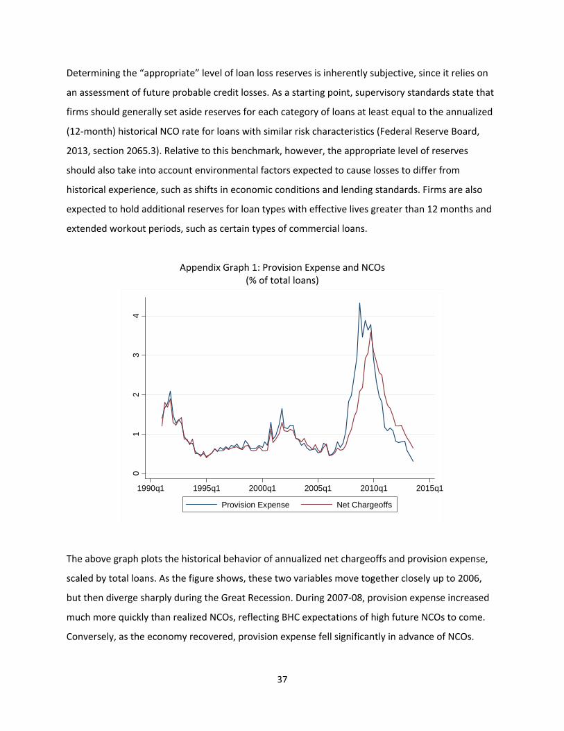
37  

Determining the “appropriate” level of loan loss reserves is inherently subjective, since it relies on 

an assessment of future probable credit losses. As a starting point, supervisory standards state that 

firms should generally set aside reserves for each category of loans at least equal to the annualized 

(12‐month) historical NCO rate for loans with similar risk characteristics (Federal Reserve Board, 

2013, section 2065.3). Relative to this benchmark, however, the appropriate level of reserves 

should also take into account environmental factors expected to cause losses to differ from 

historical experience, such as shifts in economic conditions and lending standards. Firms are also 

expected to hold additional reserves for loan types with effective lives greater than 12 months and 

extended workout periods, such as certain types of commercial loans.  

 

Appendix Graph 1: Provision Expense and NCOs (% of total loans) 

 

 

The above graph plots the historical behavior of annualized net chargeoffs and provision expense, 

scaled by total loans. As the figure shows, these two variables move together closely up to 2006, 

but then diverge sharply during the Great Recession. During 2007‐08, provision expense increased 

much more quickly than realized NCOs, reflecting BHC expectations of high future NCOs to come. 

Conversely, as the economy recovered, provision expense fell significantly in advance of NCOs. 

 

01

23

4

1990q1 1995q1 2000q1 2005q1 2010q1 2015q1

Provision Expense Net Chargeoffs

 

38  

Next we plot the level of the ALLL over time, alongside the sum of realized quarterly net chargeoffs 

over the following 12 months, as well as the average annualized NCO rate over the entire sample 

period (Box Graph 2). ALLL as a percentage of total loans trends downwards significantly between 

1990 and 2006, before rising sharply during the recession. ALLL remains elevated today compared 

to pre‐crisis levels. Note that actual ALLL almost always lies above the level predicted by a naïve 

application of the “12‐month” rule (either based on average NCOs over the entire sample period, or 

realized future NCOs over the subsequent 12 months). This appears consistent with supervisory 

guidance, which recommends that ALLL should in general be at least equal to the annualized NCO 

rate (i.e. the 12‐month rule is an approximate lower bound).  

 

Appendix Graph 2: ALLL and realized net chargeoffs (% of total loans) 

 

  

Assumptions for Reserves and Provision Expense in the CLASS Model 

Any accounting‐based stress testing model, including CLASS, must include an assumption about the 

loan loss provisioning rule used by firms. Note that for a given path of NCOs, we make an 

assumption about either ALLL or provision expense (but not both, since they are identically linked).  

 

01

23

4

1990q1 1995q1 2000q1 2005q1 2010q1 2015q1

ALLL Next 12-months NCOsAverage 12-months NCOs

 

39  

We consider three different rules for provisioning behavior. Our code allows us to toggle between 

them when calculating the capital projections. 

 

1. Provisions = NCO. Under  this approach, banks simply expense whatever net charge‐offs were 

incurred  in  the current quarter. This  is equivalent  to assuming  that  loan  loss  reserves  remain 

constant  over  the  forecast  horizon.  As  can  be  seen  above,  this  rule  is  a  reasonable 

approximation  to  bank  behavior  over  the  period  1991‐2006,  but  has  been  less  so  since  the 

financial crisis. 

2. ALLL = next four quarters of projected NCOs under the macro scenario. This rule is motivated 

by the supervisory recommendations that reserves be generally at  least equal to the historical 

annualized  NCO  rate,  and  that  the  level  of  reserves  should  be  sensitive  to macroeconomic 

conditions. Under this approach, we first forecast total NCOs in each quarter over the forecast 

horizon. We  then calculate  loan  loss  reserves as being equal  to  the next  four quarters of net 

charge‐offs. We then calculate provision expense in each quarter as: Provision expense t = NCO t 

+ [LLR t ‐ LLR t‐1 ]. 

3.   “Tunnel”: Provisions = NCO, as  long as LLR are within a range of projected NCOs. Under this 

hybrid approach, provisions are set equal to current NCOs (as in rule 1), as long as provisions do 

not deviate “too far” from being equal to the sum of future NCOs. In particular we use a range 

of 100%‐250% of projected 12‐month NCOs. 

   

  ALLL < 4 NCOs:       ALLL = 4 NCOs (and compute provisions accordingly) 

  ALLL > 250% x 4 NCOs:     ALLL = 250% x 4 NCOs (and compute provisions accordingly)  

  4 NCOs < LLR < 250% * 4 NCOs:  Provision expense = NCOs  

   

The key disadvantage of approach 1, is that setting provision expense equal to current charge‐offs is 

not  forward  looking. For example, heading  into a  recession,  loan  loss  reserves should  increase  in 

expectation of higher NCOs  in future quarters, even  if those charge‐offs have not yet occurred.  In 

contrast, approaches 2 and 3 are forward looking.  

 

 

40  

An important limitation of approach 2 (setting ALLL equal to the next four quarters of NCOs), is that 

this rule understates historical ALLL, especially during non‐recession periods, as shown in the graph 

above. Approach 3, the tunnel approach, provides one way to deal with this  issue, since  it allows 

reserves to be as much as 250% of the sum of the next four quarters of projected NCOs.  

 

A  potentially  confusing  issue  that  arises  under  approaches  2  and  3  is  that  projected  ALLL  is 

calculated using a behavioral  rule  that  is  likely  to differ  from  the most  recent historical  value of 

ALLL. For example, as can be seen under a baseline scenario, the four quarter rule (approach 2) will 

generally imply a lower projected ALLL than the most recent historical value of ALLL. Consequently, 

ALLL will shift downwards discontinuously  in the first quarter of the forecast horizon. We address 

this  issue by adjusting both  forecast and  the  current value of  reserves  to be  consistent with  the 

behavioral rule used for reserving. This  implies that the adjusted starting  level of ALLL and capital 

will differ across scenarios, and thus reserves and capital may differ across scenarios. 

 

The default provisioning rule used by  the CLASS model  is  the “tunnel”  rule described above. This 

simple rule could easily be made more sophisticated  in future versions of the CLASS model, either 

by  using  a  formula  that  is  dependent  on  the  composition  of  the  firm’s  loan  portfolio,  or  by 

estimating a formal econometric model of ALLL or provision expense. 

 

 

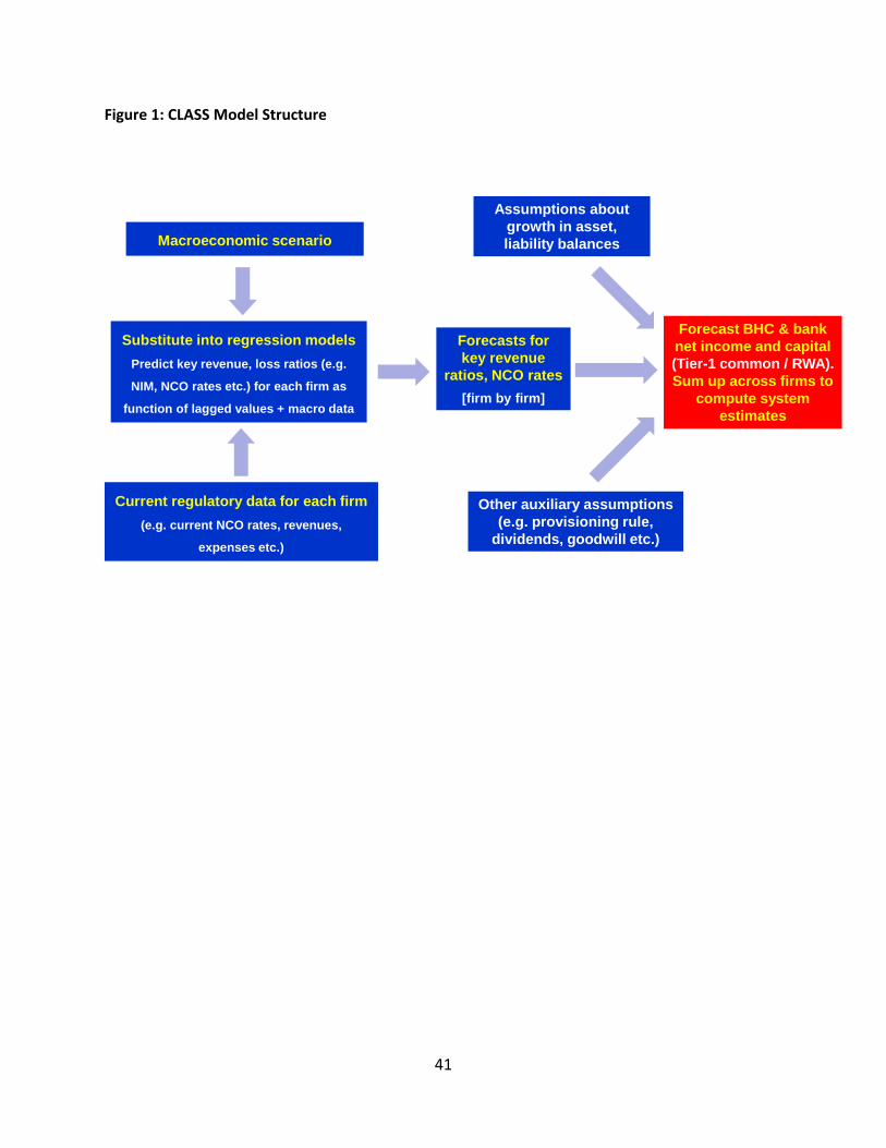
41  

Figure 1: CLASS Model Structure 

 

 

 

 

 

   

Forecasts for key revenue

ratios, NCO rates

[firm by firm]

Macroeconomic scenario

Substitute into regression models

Predict key revenue, loss ratios (e.g.

NIM, NCO rates etc.) for each firm as

function of lagged values + macro data

Current regulatory data for each firm

(e.g. current NCO rates, revenues,

expenses etc.)

Assumptions about growth in asset, liability balances

Other auxiliary assumptions (e.g. provisioning rule,

dividends, goodwill etc.)

Forecast BHC & bank net income and capital (Tier-1 common / RWA).Sum up across firms to

compute system estimates

 

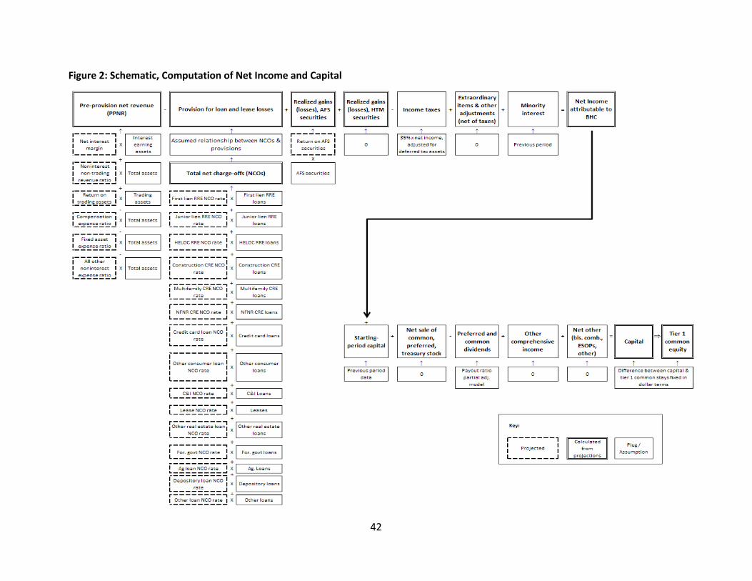
42  

Figure 2: Schematic, Computation of Net Income and Capital 

 

 

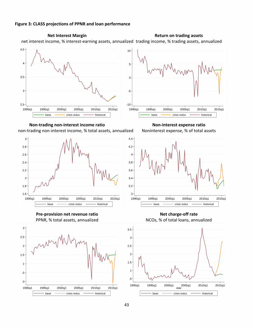
43  

Figure 3: CLASS projections of PPNR and loan performance    Net Interest Margin  Return on trading assets           net interest income, % interest‐earning assets, annualized  trading income, % trading assets, annualized 

   Non‐trading non‐interest income ratio  Non‐interest expense ratio    non‐trading non‐interest income, % total assets, annualized  Noninterest expense, % of total assets 

      Pre‐provision net revenue ratio   Net charge‐off rate     PPNR, % total assets, annualized  NCOs, % of total loans, annualized 

 

2.5

3

3.5

4

4.5

1990q1 1995q1 2000q1 2005q1 2010q1 2015q1

base crisis redux historical

-10

-5

0

5

10

1990q1 1995q1 2000q1 2005q1 2010q1 2015q1

base crisis redux historical

1.6

1.8

2

2.2

2.4

2.6

2.8

3

1990q1 1995q1 2000q1 2005q1 2010q1 2015q1

base crisis redux historical

3

3.2

3.4

3.6

3.8

4

4.2

4.4

1990q1 1995q1 2000q1 2005q1 2010q1 2015q1

base crisis redux historical

0

.5

1

1.5

2

2.5

3

1990q1 1995q1 2000q1 2005q1 2010q1 2015q1

base crisis redux historical

.5

1

1.5

2

2.5

3

3.5

1990q1 1995q1 2000q1 2005q1 2010q1 2015q1date

base crisis redux historical

 

44  

  Figure 4: Return on assets (Annualized after‐tax net income, % of total assets) 

 

 

Figure 5: Capital projections: Tier 1 common equity (percent of RWA) 

                             A. Industry aggregate                                               B. Distribution of capital across firms 

  

 

 

 

 

 

 

-2

-1.5

-1

-.5

0

.5

1

1.5

1990q1 1995q1 2000q1 2005q1 2010q1 2015q1

base crisis redux historical

56

78

910

1112

2000q1 2005q1 2010q1 2015q1

base crisis redux historical

020

4060

8010

0%

indu

stry

ass

ets

5 10 15

base crisis redux

 

45  

 

 

Figure 6: Evolution of industry capital “gap” 

A. Relative to 8% Tier 1 common / RWA threshold 

  

B. Relative to a 5% Tier 1 common / RWA threshold 

 

010

020

030

040

050

0C

api

tal G

ap

($bn

), 8

% T

hre

shol

d

2002q1 2004q1 2006q1 2008q1 2010q1 2012q1

010

020

030

040

050

0C

api

tal G

ap

($bn

), 5

% T

hre

shol

d

2002q1 2004q1 2006q1 2008q1 2010q1 2012q1

 

46  

Figure 7: Correlates of Change in Capital Ratio During Crisis Redux Scenario 

Y‐axis is the difference between the end‐of‐crisis‐redux tier 1 common equity ratio for each firm and its historical 

2013:Q3 capital ratio. The size of each circle reflects the 2013:Q3 assets of the firm. Lines of best fit are based on 

least squares using data winsorized at 1% and 99% values. 

A. Projected capital decline vs 2013:Q3 capital ratio          B. Projected capital decline vs liquid assets ratio 

 

    C. Projected capital decline vs RWA / total assets                  D. Projected capital decline vs firm size 

 

-6-4

-20

2T

ier

1 C

om

mo

n D

rop

(win

soris

ed a

t 1%

)

0 10 20 30 40Tier 1 Common: Last Historical (winsorised at 1%)

Note: The regression line is the fitted values of an OLS regressionNote: Marker size represents total assets.

-6-4

-20

2T

ier

1 C

om

mo

n D

rop

(win

soris

ed a

t 1%

)

0 20 40 60Cash + IBB + Securities + Fed Funds, % of Assets, Last Historical (winsorised at

Note: The regression line is the fitted values of an OLS regressionNote: Marker size represents total assets.

-6-4

-20

2T

ier

1 C

om

mo

n D

rop

(win

soris

ed a

t 1%

)

.4 .6 .8 1RWA/Total Assets, Last Historical (winsorised at 1%)

Note: The regression line is the fitted values of an OLS regressionNote: Marker size represents total assets.

-6-4

-20

2T

ier

1 C

om

mo

n D

rop

(win

soris

ed a

t 1%

)

0 2 4 6 8Log Total Assets (ln(Billions)), Last Historical (winsorised at 1%)

 

47  

Figure 8: Sensitivity to assumptions  A. Asset growth rate 

 B. Provisioning assumption 

 C. Payout rule 

      

67

89

1011

12T

ier

1 C

omm

on R

atio

2000q1 2005q1 2010q1 2015q1

Historical 0.00% 1.25%2.50% -1.25%

67

89

1011

12T

ier

1 C

omm

on R

atio

2000q1 2005q1 2010q1 2015q1

Historical NCOFour Quarter Tunnel

67

89

1011

12T

ier

1 C

omm

on R

atio

2000q1 2005q1 2010q1 2015q1

Historical Zero DividendsNo Change in Dividends Benchmark CLASS rule, (d=0.9)

 

48  

Table 1: Comparison and Differences Between Stress Test Frameworks  

  CLASS Model DFAST/CCAR 

Modeling Approach  Top‐down models based on outcomes (net charge‐offs) for 

broad loan and securities portfolio segments 

Bottom‐up models focused on the risk characteristics of individual loans, securities, and trading 

positions 

Data  Publicly available balance sheet and income statement regulatory report data from Call and Y‐9C 

filings 

Detailed supervisory information from individual BHCs, often at the 

level of individual loans or securities 

Coverage  The 200 largest BHCs and independent banks, plus the rest of the industry. Results reported at the aggregate industry level 

BHCs with assets exceeding $50 billion (starting in 2014). Results reported in the aggregate and at 

the individual BHC level 

Trading and Counterparty  Trading revenue modeled based on the macroeconomic scenario 

Separate instantaneous global market shock on the trading and counterparty positions of the 6 

largest BHCs 

Dividends  Stylized assumptions that result in dividends varying with BHC 

performance and macroeconomic conditions 

For DFAST, stylized assumptions that hold dividends fixed at recent historical levels 

Balance Sheet Growth  Stylized assumption for all institutions in all scenarios 

Varies across institutions and across scenarios 

Risk Weighted Assets  Changes proportionately with the balance sheet, implicitly carrying forward prevailing regulatory 

capital rules 

Changes with the macroeconomic scenario, incorporating the phase‐in of any new regulatory capital 

rules  

Regulatory Capital Model  Captures key elements, but involves approximations of certain 

complex calculations 

More detailed and precise calculations of regulatory capital 

 

49  

Table 2: Summary Statistics of Macroeconomic Variables

Variable Definition 2013:Q3 Value

Historical Mean

Historical

SD

Term Spread (10 year minus 3 months, pct. pt) 10 . 3 . 2.70 2.09 1.16

Quarterly growth in Stock market returns (%, log change) 100 5.49 1.92 8.50

Annualized Real GDP growth (%) 400 1.98 2.51 2.49

Annualized Change in the Civilian Unemployment Rate (%) % % 4 -1.20 0.05 1.20

3 Month Treasury Yield (%) 3 0.00 3.00 2.06

Spread of BBB Bond Index to 10 Year Treasury Yield in Percent 10 . 2.20 1.72 0.92

Quarterly change in BBB bond spread (pct. pt) 0.10 0.00 0.42

Quarterly change in 10 year Treasury yield (pct. pt) 10 . 10 . 0.70 -0.06 0.38

Annual House Price Index (log change) 100 9.85 3.13 7.55

Annual Commercial Property Price Index (log change) 100 7.61 2.95 11.76

 

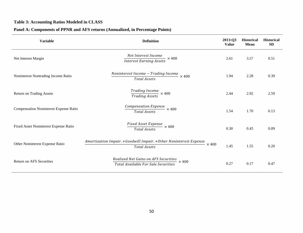
50  

Table 3: Accounting Ratios Modeled in CLASS

Panel A: Components of PPNR and AFS returns (Annualized, in Percentage Points)

Variable Definition 2013:Q3 Value

Historical Mean

Historical SD

Net Interest Margin 400 2.61 3.57 0.51

Noninterest Nontrading Income Ratio 400 1.94 2.28 0.39

Return on Trading Assets 400 2.44 2.92 2.59

Compensation Noninterest Expense Ratio 400 1.54 1.70 0.13

Fixed Asset Noninterest Expense Ratio 400 0.30 0.45 0.09

Other Noninterest Expense Ratio . .

400 1.45 1.55 0.20

Return on AFS Securities 400 0.27 0.17 0.47

 

 

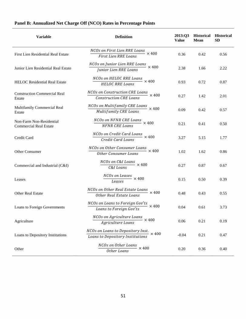
51  

Panel B: Annualized Net Charge Off (NCO) Rates in Percentage Points

Variable Definition

2013:Q3 Value

Historical Mean

Historical SD

First Lien Residential Real Estate 400 0.36 0.42 0.56

Junior Lien Residential Real Estate 400 2.38 1.66 2.22

HELOC Residential Real Estate 400 0.93 0.72 0.87

Construction Commercial Real Estate

400 0.27 1.42 2.01

Multifamily Commercial Real Estate

400 0.09 0.42 0.57

Non-Farm Non-Residential Commercial Real Estate

400 0.21 0.41 0.50

Credit Card 400 3.27 5.15 1.77

Other Consumer

400 1.02 1.62 0.86

Commercial and Industrial (C&I) &

& 400 0.27 0.87 0.67

Leases 400 0.15 0.50 0.39

Other Real Estate

400 0.48 0.43 0.55

Loans to Foreign Governments ′

′ 400 0.04 0.61 3.73

Agriculture 400 0.06 0.21 0.19

Loans to Depository Institutions . 400 -0.04 0.21 0.47

Other 400 0.20 0.36 0.40

 

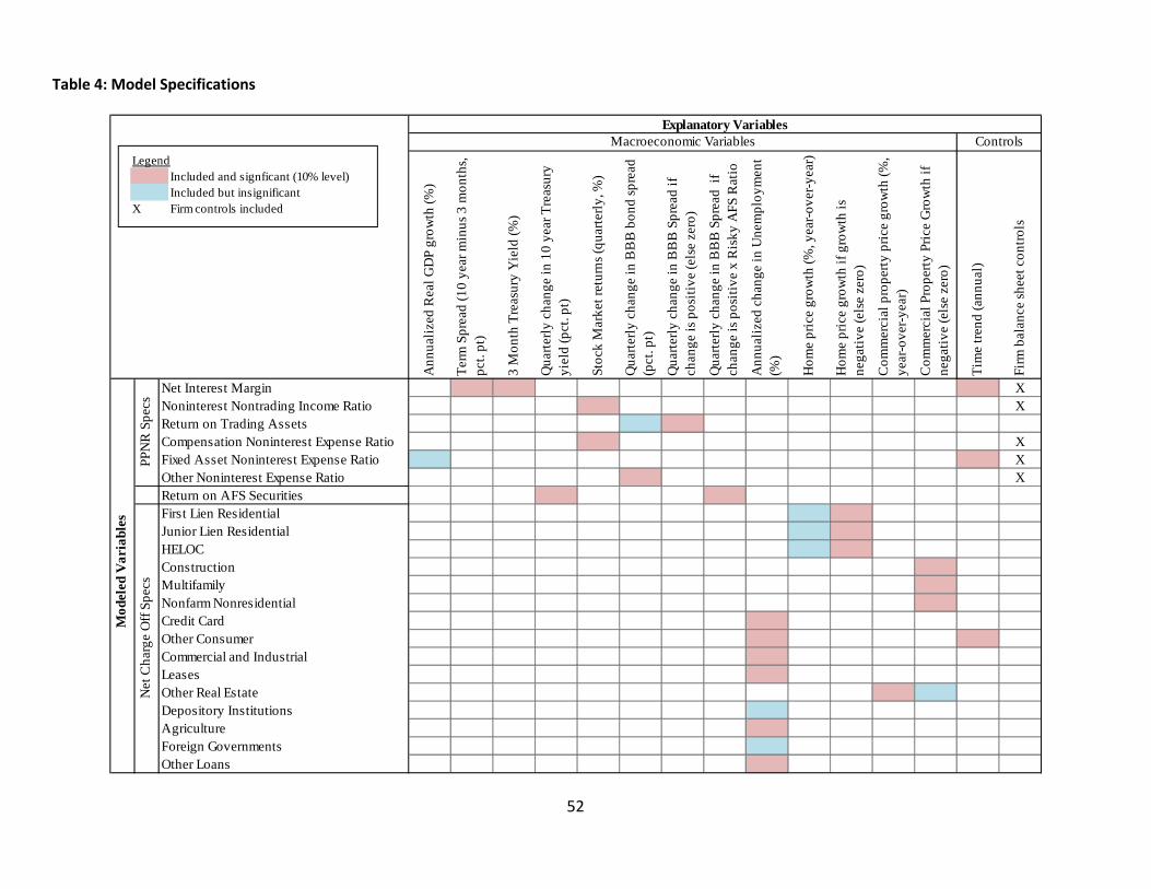
52  

Table 4: Model Specifications  

 

Ann

uali

zed

Rea

l GD

P gr

owth

(%)

Ter

m S

prea

d (1

0 ye

ar m

inus

3 m

onth

s,

pct.

pt)

3 M

onth

Tre

asur

y Y

ield

(%)

Qua

rter

ly c

hang

e in

10

year

Tre

asur

y yi

eld

(pct

. pt)

Stoc

k M

arke

t ret

urns

(qua

rter

ly, %

)

Qua

rter

ly c

hang

e in

BB

B b

ond

spre

ad

(pct

. pt)

Qua

rter

ly c

hang

e in

BB

B S

prea

d if

ch

ange

is p

osit

ive

(els

e ze

ro)

Qua

rter

ly c

hang

e in

BB

B S

prea

d if

ch

ange

is p

osit

ive

x R

isky

AFS

Rat

io

Ann

uali

zed

chan

ge in

Une

mpl

oym

ent

(%)

Hom

e pr

ice

grow

th (%

, yea

r-ov

er-y

ear)

Hom

e pr

ice

grow

th if

gro

wth

is

nega

tive

(els

e ze

ro)

Com

mer

cial

pro

pert

y pr

ice

grow

th (%

, ye

ar-o

ver-

year

)

Com

mer

cial

Pro

pert

y Pr

ice

Gro

wth

if

nega

tive

(els

e ze

ro)

Tim

e tr

end

(ann

ual)

Firm

bal

ance

she

et c

ontr

ols

Net Interest Margin XNoninterest Nontrading Income Ratio XReturn on Trading AssetsCompensation Noninterest Expense Ratio XFixed Asset Noninterest Expense Ratio XOther Noninterest Expense Ratio XReturn on AFS SecuritiesFirst Lien ResidentialJunior Lien ResidentialHELOCConstructionMultifamilyNonfarm NonresidentialCredit CardOther ConsumerCommercial and IndustrialLeasesOther Real EstateDepository InstitutionsAgricultureForeign GovernmentsOther Loans

Explanatory VariablesM

odel

ed V

aria

bles

PPN

R S

pecs

Net

Cha

rge

Off

Spe

csMacroeconomic Variables Controls

LegendIncluded and signficant (10% level)Included but insignificant

X Firm controls included

 

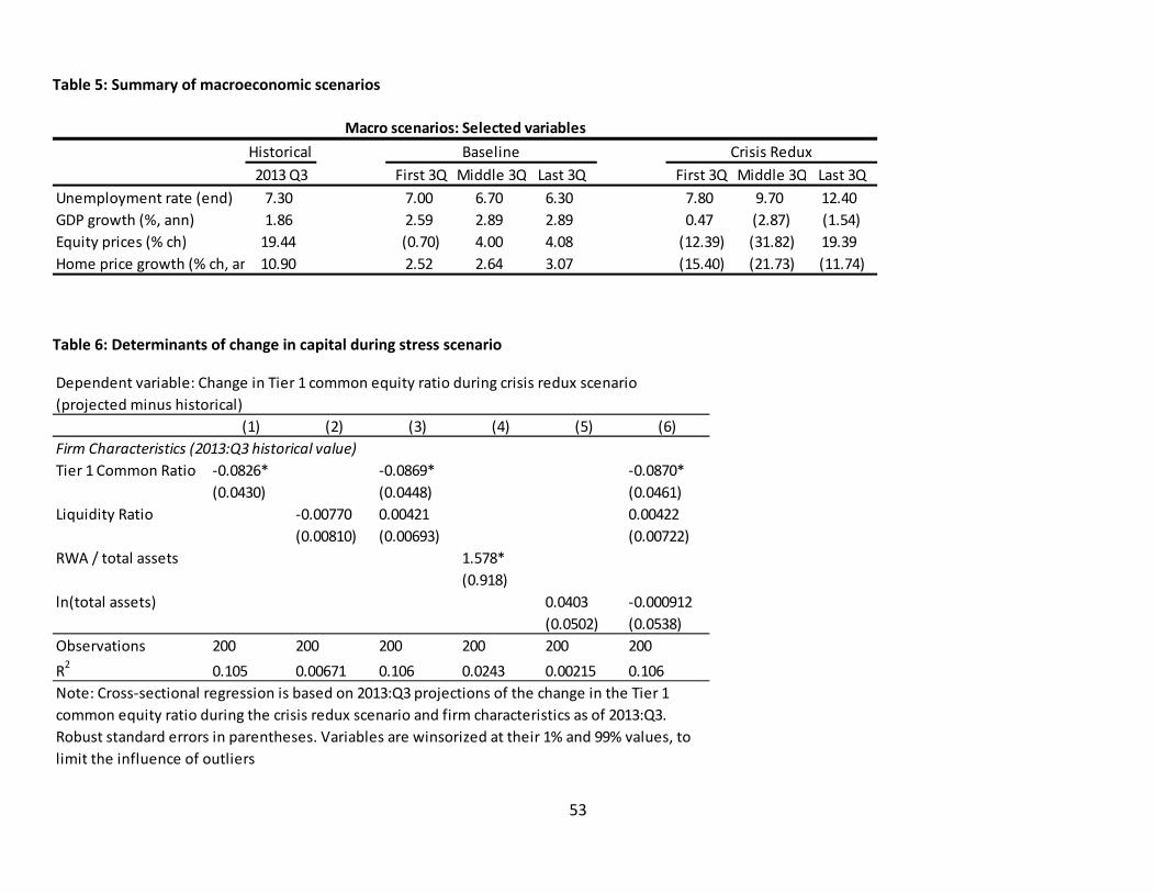
53  

Table 5: Summary of macroeconomic scenarios  

   

Table 6: Determinants of change in capital during stress scenario 

 

Historical

2013 Q3 First 3Q Middle 3Q Last 3Q First 3Q Middle 3Q Last 3Q

Unemployment rate (end) 7.30 7.00 6.70 6.30 7.80 9.70 12.40

GDP growth (%, ann) 1.86 2.59 2.89 2.89 0.47 (2.87) (1.54)

Equity prices (% ch) 19.44 (0.70) 4.00 4.08 (12.39) (31.82) 19.39

Home price growth (% ch, an 10.90 2.52 2.64 3.07 (15.40) (21.73) (11.74)

Baseline Crisis Redux

Macro scenarios: Selected variables

(1) (2) (3) (4) (5) (6)

Firm Characteristics (2013:Q3 historical value)

Tier 1 Common Ratio ‐0.0826* ‐0.0869* ‐0.0870*

(0.0430) (0.0448) (0.0461)

Liquidity Ratio ‐0.00770 0.00421 0.00422

(0.00810) (0.00693) (0.00722)

RWA / total assets 1.578*

(0.918)

ln(total assets) 0.0403 ‐0.000912

(0.0502) (0.0538)

Observations 200 200 200 200 200 200

R2

0.105 0.00671 0.106 0.0243 0.00215 0.106

Note: Cross‐sectional regression is based on 2013:Q3 projections of the change in the Tier 1 

common equity ratio during the crisis redux scenario and firm characteristics as of 2013:Q3. 

Robust standard errors in parentheses. Variables are winsorized at their 1% and 99% values, to 

limit the influence of outliers

Dependent variable: Change in Tier 1 common equity ratio during crisis redux scenario 

(projected minus historical)