CLAMI: Defect Prediction on Unlabeled Datasetslifove.github.io/files/CLAMI_ASE.pdf · CLAMI: Defect Prediction on Unlabeled Datasets Jaechang Nam and Sunghun Kim Department of Computer

CLAMI: Defect Prediction on Unlabeled Datasets

Jaechang Nam and Sunghun KimDepartment of Computer Science and Engineering

The Hong Kong University of Science and Technology, Hong Kong, ChinaEmail: {jcnam,hunkim}@cse.ust.hk

Abstract—Defect prediction on new projects or projects withlimited historical data is an interesting problem in softwareengineering. This is largely because it is difficult to collect defectinformation to label a dataset for training a prediction model.Cross-project defect prediction (CPDP) has tried to address thisproblem by reusing prediction models built by other projectsthat have enough historical data. However, CPDP does notalways build a strong prediction model because of the differentdistributions among datasets. Approaches for defect predictionon unlabeled datasets have also tried to address the problem byadopting unsupervised learning but it has one major limitation,the necessity for manual effort.

In this study, we propose novel approaches, CLA and CLAMI,that show the potential for defect prediction on unlabeled datasetsin an automated manner without need for manual effort. The keyidea of the CLA and CLAMI approaches is to label an unlabeleddataset by using the magnitude of metric values. In our empiricalstudy on seven open-source projects, the CLAMI approach ledto the promising prediction performances, 0.636 and 0.723 inaverage f-measure and AUC, that are comparable to those ofdefect prediction based on supervised learning.

I. INTRODUCTION

Defect prediction plays an important role in software qual-ity [1]. Defect prediction techniques provide a list of defect-prone source code so that quality assurance (QA) teams canfocus on the most defective parts of their products in advance.In this way, QA teams can effectively allocate limited resourceson which to review and test their software products beforereleasing them. In industry, defect prediction techniques havebeen actively adopted for software quality assurance [2], [3],[4], [5], [6].

Researchers have proposed and facilitated various defectprediction algorithms and metrics [1], [4], [7], [8], [9], [10],[11], [12], [13], [14], [15], [16], [17], [18]. Most defect predic-tion models are based on supervised learning for classification(e.g., predicting defect-proneness of a source code file) orregression (e.g., predicting the number of defects in a sourcecode file) [1], [17], [18], [19]. Rather than using a machinelearning technique, Kim et al. proposed BugCache, whichmanages defect-prone entities in source code by adapting thecache concept used in operating system [12]. Metrics for defectprediction can be divided into code and process metrics [20].Code metrics represent how the source code is complex whileprocess metrics represent how the development process iscomplex [1], [20].

In particular, studies on defect prediction metrics havebeen actively conducted as the use of software archives suchas version control systems and issue trackers has becomepopular [20]. Most metrics proposed over the last decade suchas change/code metric churn, change/code entropy, popularity,

and developer interaction have been collected from varioussoftware archives [7], [9], [10], [11], [13], [16], [17].

However, typical defect prediction techniques based onsupervised learning are designed for a single software projectand are difficult to apply to new projects or projects that havelimited historical data in software archives. Defect predictionmodels based on supervised learning can be constructed byusing a dataset with actual defect information, that is, alabeled dataset. Defect information usually accumulates in thesoftware archives, thus new projects or projects with a shortdevelopment history do not have enough defect information.This is a major limitation of the typical defect predictiontechniques based on supervised learning.

To address this limitation, researchers have proposed vari-ous approaches to enable defect prediction on projects withlimited historical data. Cross-project defect prediction thatbuilds a prediction model using data from other projects hasbeen studied by many researchers [19], [21], [22], [23], [24],[25], [26], [27]. Defect prediction techniques on unlabeleddatasets were proposed as well [28], [29]. Recently, an ap-proach to build a universal defect prediction model by usingmultiple project datasets was introduced [30].

However, there is still an issue of different distributionsamong datasets in existing approaches for cross-project defectprediction (CPDP) and universal defect prediction (UDP). InCPDP and UDP, the major task is to make the differentdistributions of datasets similar since prediction models workwell when the datasets for training and testing a model have thesame distributions [31], [32]. However, the approaches basedon making the different distributions similar between trainingand test datasets may not always be effective [22], [23].

Compared to CPDP and UDP, the existing approachesfor defect prediction on unlabeled datasets are relatively lessaffected by the issue of different distributions among datasetsbut will always require manual effort by human experts [28],[29]. Zhong et al. proposed the expert-based defect predictionon unlabeled datasets where a human expert would labelclusters from an unlabeled dataset after clustering [29]. Catalet al. proposed the threshold-based approach where labelingdatasets is conducted based on a certain threshold value of ametric [28]. A proper metric threshold for the threshold-basedapproach is decided by the intervention of human experts [28].Since these approaches on unlabeled datasets are conducted onthe test dataset itself, the issue of the different distributionsamong datasets is not affected [28], [29]. However, theseapproaches require manual effort by human experts [28], [29].

The goal of this study is to propose novel approaches,CLA and CLAMI, which can conduct defect prediction on

Classification

Software Archives

9"8"5"6"B"1"2"3"1"C"0"1"4"5"C"

8"7"5"9"B"

...

Instances with Metrics and Labels

9"8"5"B"1"2"3"C"

8"7"5"B"

...

Training Instances

(Preprocessing)

Model

7"9"9"?"New Instance Generate

Instances Build

a Model

0"1"4"C"

7"9"9"B"

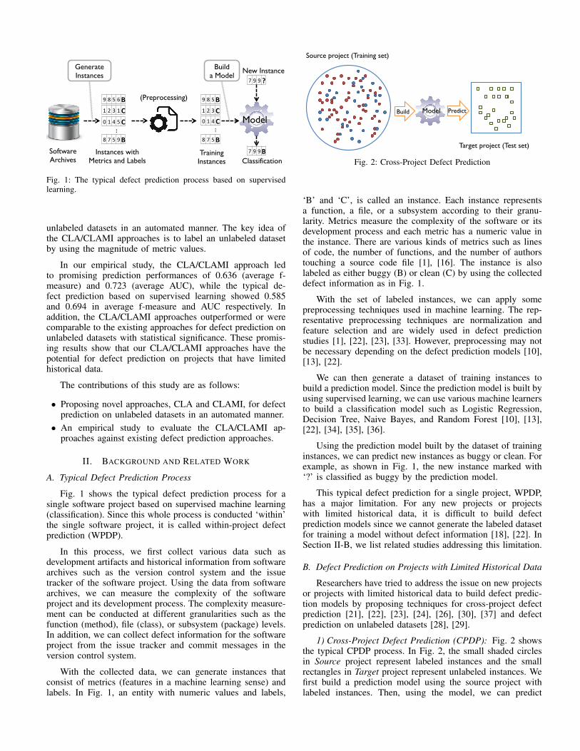
Fig. 1: The typical defect prediction process based on supervisedlearning.

unlabeled datasets in an automated manner. The key idea ofthe CLA/CLAMI approaches is to label an unlabeled datasetby using the magnitude of metric values.

In our empirical study, the CLA/CLAMI approach ledto promising prediction performances of 0.636 (average f-measure) and 0.723 (average AUC), while the typical de-fect prediction based on supervised learning showed 0.585and 0.694 in average f-measure and AUC respectively. Inaddition, the CLA/CLAMI approaches outperformed or werecomparable to the existing approaches for defect prediction onunlabeled datasets with statistical significance. These promis-ing results show that our CLA/CLAMI approaches have thepotential for defect prediction on projects that have limitedhistorical data.

The contributions of this study are as follows:

• Proposing novel approaches, CLA and CLAMI, for defectprediction on unlabeled datasets in an automated manner.• An empirical study to evaluate the CLA/CLAMI ap-

proaches against existing defect prediction approaches.

II. BACKGROUND AND RELATED WORK

A. Typical Defect Prediction Process

Fig. 1 shows the typical defect prediction process for asingle software project based on supervised machine learning(classification). Since this whole process is conducted ‘within’the single software project, it is called within-project defectprediction (WPDP).

In this process, we first collect various data such asdevelopment artifacts and historical information from softwarearchives such as the version control system and the issuetracker of the software project. Using the data from softwarearchives, we can measure the complexity of the softwareproject and its development process. The complexity measure-ment can be conducted at different granularities such as thefunction (method), file (class), or subsystem (package) levels.In addition, we can collect defect information for the softwareproject from the issue tracker and commit messages in theversion control system.

With the collected data, we can generate instances thatconsist of metrics (features in a machine learning sense) andlabels. In Fig. 1, an entity with numeric values and labels,

Cross prediction model

4

Target project (Test set)

Source project (Training set)

Model Build Predict

Fig. 2: Cross-Project Defect Prediction

‘B’ and ‘C’, is called an instance. Each instance representsa function, a file, or a subsystem according to their granu-larity. Metrics measure the complexity of the software or itsdevelopment process and each metric has a numeric value inthe instance. There are various kinds of metrics such as linesof code, the number of functions, and the number of authorstouching a source code file [1], [16]. The instance is alsolabeled as either buggy (B) or clean (C) by using the collecteddefect information as in Fig. 1.

With the set of labeled instances, we can apply somepreprocessing techniques used in machine learning. The rep-resentative preprocessing techniques are normalization andfeature selection and are widely used in defect predictionstudies [1], [22], [23], [33]. However, preprocessing may notbe necessary depending on the defect prediction models [10],[13], [22].

We can then generate a dataset of training instances tobuild a prediction model. Since the prediction model is built byusing supervised learning, we can use various machine learnersto build a classification model such as Logistic Regression,Decision Tree, Naive Bayes, and Random Forest [10], [13],[22], [34], [35], [36].

Using the prediction model built by the dataset of traininginstances, we can predict new instances as buggy or clean. Forexample, as shown in Fig. 1, the new instance marked with‘?’ is classified as buggy by the prediction model.

This typical defect prediction for a single project, WPDP,has a major limitation. For any new projects or projectswith limited historical data, it is difficult to build defectprediction models since we cannot generate the labeled datasetfor training a model without defect information [18], [22]. InSection II-B, we list related studies addressing this limitation.

B. Defect Prediction on Projects with Limited Historical Data

Researchers have tried to address the issue on new projectsor projects with limited historical data to build defect predic-tion models by proposing techniques for cross-project defectprediction [21], [22], [23], [24], [26], [30], [37] and defectprediction on unlabeled datasets [28], [29].

1) Cross-Project Defect Prediction (CPDP): Fig. 2 showsthe typical CPDP process. In Fig. 2, the small shaded circlesin Source project represent labeled instances and the smallrectangles in Target project represent unlabeled instances. Wefirst build a prediction model using the source project withlabeled instances. Then, using the model, we can predict

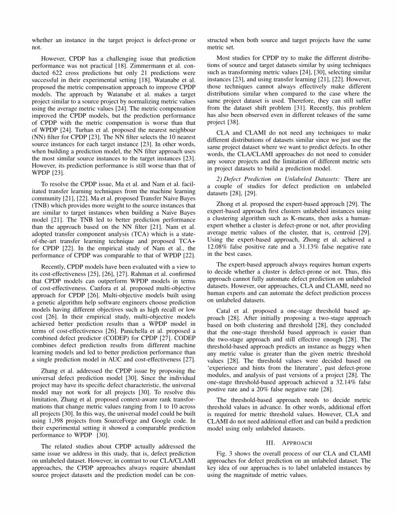
whether an instance in the target project is defect-prone ornot.

However, CPDP has a challenging issue that predictionperformance was not practical [18]. Zimmermann et al. con-ducted 622 cross predictions but only 21 predictions weresuccessful in their experimental setting [18]. Watanabe et al.proposed the metric compensation approach to improve CPDPmodels. The approach by Watanabe et al. makes a targetproject similar to a source project by normalizing metric valuesusing the average metric values [24]. The metric compensationimproved the CPDP models, but the prediction performanceof CPDP with the metric compensation is worse than thatof WPDP [24]. Turhan et al. proposed the nearest neighbour(NN) filter for CPDP [23]. The NN filter selects the 10 nearestsource instances for each target instance [23]. In other words,when building a prediction model, the NN filter approach usesthe most similar source instances to the target instances [23].However, its prediction performance is still worse than that ofWPDP [23].

To resolve the CPDP issue, Ma et al. and Nam et al. facil-itated transfer learning techniques from the machine learningcommunity [21], [22]. Ma et al. proposed Transfer Naive Bayes(TNB) which provides more weight to the source instances thatare similar to target instances when building a Naive Bayesmodel [21]. The TNB led to better prediction performancethan the approach based on the NN filter [21]. Nam et al.adopted transfer component analysis (TCA) which is a state-of-the-art transfer learning technique and proposed TCA+for CPDP [22]. In the empirical study of Nam et al., theperformance of CPDP was comparable to that of WPDP [22].

Recently, CPDP models have been evaluated with a view toits cost-effectiveness [25], [26], [27]. Rahman et al. confirmedthat CPDP models can outperform WPDP models in termsof cost-effectiveness. Canfora et al. proposed multi-objectiveapproach for CPDP [26]. Multi-objective models built usinga genetic algorithm help software engineers choose predictionmodels having different objectives such as high recall or lowcost [26]. In their empirical study, multi-objective modelsachieved better prediction results than a WPDP model interms of cost-effectiveness [26]. Panichella et al. proposed acombined defect predictor (CODEP) for CPDP [27]. CODEPcombines defect prediction results from different machinelearning models and led to better prediction performance thana single prediction model in AUC and cost-effectiveness [27].

Zhang et al. addressed the CPDP issue by proposing theuniversal defect prediction model [30]. Since the individualproject may have its specific defect characteristic, the universalmodel may not work for all projects [30]. To resolve thislimitation, Zhang et al. proposed context-aware rank transfor-mations that change metric values ranging from 1 to 10 acrossall projects [30]. In this way, the universal model could be builtusing 1,398 projects from SourceForge and Google code. Intheir experimental setting it showed a comparable predictionperformance to WPDP [30].

The related studies about CPDP actually addressed thesame issue we address in this study, that is, defect predictionon unlabeled dataset. However, in contrast to our CLA/CLAMIapproaches, the CPDP approaches always require abundantsource project datasets and the prediction model can be con-

structed when both source and target projects have the samemetric set.

Most studies for CPDP try to make the different distribu-tions of source and target datasets similar by using techniquessuch as transforming metric values [24], [30], selecting similarinstances [23], and using transfer learning [21], [22]. However,those techniques cannot always effectively make differentdistributions similar when compared to the case where thesame project dataset is used. Therefore, they can still sufferfrom the dataset shift problem [31]. Recently, this problemhas also been observed even in different releases of the sameproject [38].

CLA and CLAMI do not need any techniques to makedifferent distributions of datasets similar since we just use thesame project dataset where we want to predict defects. In otherwords, the CLA/CLAMI approaches do not need to considerany source projects and the limitation of different metric setsin project datasets to build a prediction model.

2) Defect Prediction on Unlabeled Datasets: There area couple of studies for defect prediction on unlabeleddatasets [28], [29].

Zhong et al. proposed the expert-based approach [29]. Theexpert-based approach first clusters unlabeled instances usinga clustering algorithm such as K-means, then asks a human-expert whether a cluster is defect-prone or not, after providingaverage metric values of the cluster, that is, centroid [29].Using the expert-based approach, Zhong et al. achieved a12.08% false positive rate and a 31.13% false negative ratein the best cases.

The expert-based approach always requires human expertsto decide whether a cluster is defect-prone or not. Thus, thisapproach cannot fully automate defect prediction on unlabeleddatasets. However, our approaches, CLA and CLAMI, need nohuman experts and can automate the defect prediction processon unlabeled datasets.

Catal et al. proposed a one-stage threshold based ap-proach [28]. After initially proposing a two-stage approachbased on both clustering and threshold [28], they concludedthat the one-stage threshold based approach is easier thanthe two-stage approach and still effective enough [28]. Thethreshold-based approach predicts an instance as buggy whenany metric value is greater than the given metric thresholdvalues [28]. The threshold values were decided based on‘experience and hints from the literature’, past defect-pronemodules, and analysis of past versions of a project [28]. Theone-stage threshold-based approach achieved a 32.14% falsepostive rate and a 20% false negative rate [28].

The threshold-based approach needs to decide metricthreshold values in advance. In other words, additional effortis required for metric threshold values. However, CLA andCLAMI do not need additional effort and can build a predictionmodel using only unlabeled datasets.

III. APPROACH

Fig. 3 shows the overall process of our CLA and CLAMIapproaches for defect prediction on an unlabeled dataset. Thekey idea of our approaches is to label unlabeled instances byusing the magnitude of metric values.

CLAMI Approach Overview

69

Unlabeled Dataset

(1) Clustering (2) Labeling (3) Metric Selection (4) Instance Selection

(5) Metric Selection

CLAMI Model

Build

Predict

Training dataset

Test dataset

CLA Model

(1) Clustering (2) Labeling

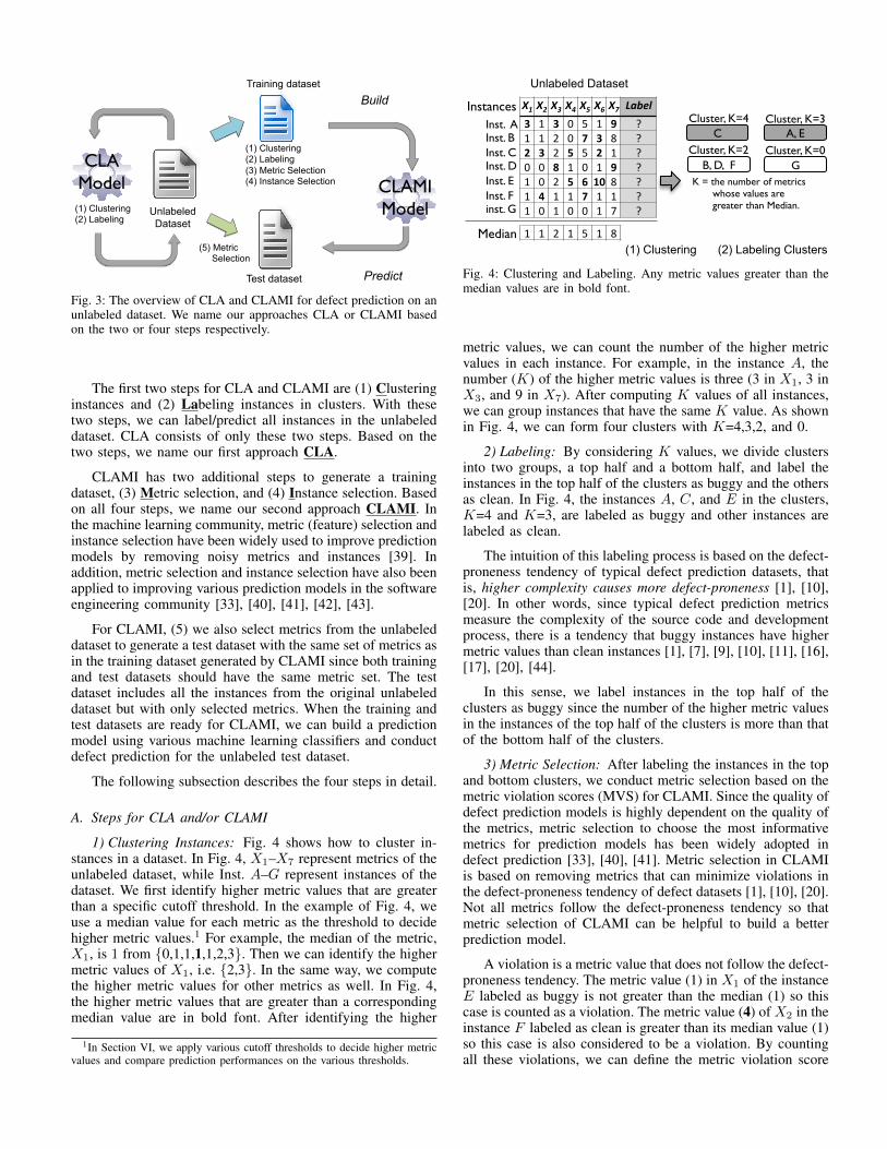
Fig. 3: The overview of CLA and CLAMI for defect prediction on anunlabeled dataset. We name our approaches CLA or CLAMI basedon the two or four steps respectively.

The first two steps for CLA and CLAMI are (1) Clusteringinstances and (2) Labeling instances in clusters. With thesetwo steps, we can label/predict all instances in the unlabeleddataset. CLA consists of only these two steps. Based on thetwo steps, we name our first approach CLA.

CLAMI has two additional steps to generate a trainingdataset, (3) Metric selection, and (4) Instance selection. Basedon all four steps, we name our second approach CLAMI. Inthe machine learning community, metric (feature) selection andinstance selection have been widely used to improve predictionmodels by removing noisy metrics and instances [39]. Inaddition, metric selection and instance selection have also beenapplied to improving various prediction models in the softwareengineering community [33], [40], [41], [42], [43].

For CLAMI, (5) we also select metrics from the unlabeleddataset to generate a test dataset with the same set of metrics asin the training dataset generated by CLAMI since both trainingand test datasets should have the same metric set. The testdataset includes all the instances from the original unlabeleddataset but with only selected metrics. When the training andtest datasets are ready for CLAMI, we can build a predictionmodel using various machine learning classifiers and conductdefect prediction for the unlabeled test dataset.

The following subsection describes the four steps in detail.

A. Steps for CLA and/or CLAMI

1) Clustering Instances: Fig. 4 shows how to cluster in-stances in a dataset. In Fig. 4, X1–X7 represent metrics of theunlabeled dataset, while Inst. A–G represent instances of thedataset. We first identify higher metric values that are greaterthan a specific cutoff threshold. In the example of Fig. 4, weuse a median value for each metric as the threshold to decidehigher metric values.1 For example, the median of the metric,X1, is 1 from {0,1,1,1,1,2,3}. Then we can identify the highermetric values of X1, i.e. {2,3}. In the same way, we computethe higher metric values for other metrics as well. In Fig. 4,the higher metric values that are greater than a correspondingmedian value are in bold font. After identifying the higher

1In Section VI, we apply various cutoff thresholds to decide higher metricvalues and compare prediction performances on the various thresholds.

{X1,X4}''

Cluster, K=3

Unlabeled Dataset

X1# X2# X3# X4# X5# X6# X7# Label#3" 1' 3" 0' 5' 1' 9" ?'1' 1' 2' 0' 7" 3" 8' ?'2" 3" 2' 5" 5' 2" 1' ?'0' 0' 8" 1' 0' 1' 9" ?'1' 0' 2' 5" 6" 10" 8' ?'1' 4" 1' 1' 7" 1' 1' ?'1' 0' 1' 0' 0' 1' 7' ?'

1' 1' 2' 1' 5' 1' 8'Median

Inst. A Inst. B Inst. C Inst. D Inst. E Inst. F inst. G

Instances

K = the number of metrics whose values are greater than Median.

C Cluster, K=4

A, E

B, D, F Cluster, K=2

G Cluster, K=0

(1) Clustering

(4) Instance Selection

X1# X2# X3# X4# X5# X6# X7# Label#3" 1' 3" 0' 5' 1' 9" Buggy"1' 1' 2' 0' 7" 3" 8' Clean"2" 3" 2' 5" 5' 2" 1' Buggy'0' 0' 8" 1' 0' 1' 9" Clean'1' 0' 2' 5" 6" 10" 8' Buggy"1' 4" 1' 1' 7" 1' 1' Clean'1' 0' 1' 0' 0' 1' 7' Clean'

Inst. A Inst. B Inst. C Inst. D Inst. E Inst. F Inst. G

1'–'7'

3'–'7'

3'–'7'

1'–'7'

4'–'7'

2'–'7'

3'–'7'

X1# X5# X7# Label#3" 5" 9" Buggy"1' 7" 8" Buggy"2' 5" 1' Clean'1' 0' 9" Clean'5" 5" 8" Buggy"0' 2' 1' Clean'

X1# X5# X7# Label#3" 5" 9" Buggy"5" 5" 8" Buggy"0' 2' 1' Clean'

Final Training Dataset

(2) Labeling Clusters

Instance Conflicts

1/7# 2/7# 3/7# 4/7#1' 3' 3' 4'0' 1' 1' 2'0' 0' 1' 3'0' 0' 1' 2'0' 1' 2' 4'1' 1' 1' 1'0' 0' 0' 1'

Metric Conflict Scores

1/7' 2/7' 3/7' 4/7'

Selected'Metrics'

X1#X4# Label#3" 0' Buggy"1' 0' Clean"2" 5" Buggy'0' 1' Clean'1' 5" Buggy"1' 1' Clean'1' 0' Clean'


2'–'7'

X1# X4# Label#1' 0' Clean"2" 5" Buggy'0' 1' Clean'1' 1' Clean'1' 0' Clean'

Inst. B Inst. C Inst. D Inst. F Inst. G


Fig. 4: Clustering and Labeling. Any metric values greater than themedian values are in bold font.

metric values, we can count the number of the higher metricvalues in each instance. For example, in the instance A, thenumber (K) of the higher metric values is three (3 in X1, 3 inX3, and 9 in X7). After computing K values of all instances,we can group instances that have the same K value. As shownin Fig. 4, we can form four clusters with K=4,3,2, and 0.

2) Labeling: By considering K values, we divide clustersinto two groups, a top half and a bottom half, and label theinstances in the top half of the clusters as buggy and the othersas clean. In Fig. 4, the instances A, C, and E in the clusters,K=4 and K=3, are labeled as buggy and other instances arelabeled as clean.

The intuition of this labeling process is based on the defect-proneness tendency of typical defect prediction datasets, thatis, higher complexity causes more defect-proneness [1], [10],[20]. In other words, since typical defect prediction metricsmeasure the complexity of the source code and developmentprocess, there is a tendency that buggy instances have highermetric values than clean instances [1], [7], [9], [10], [11], [16],[17], [20], [44].

In this sense, we label instances in the top half of theclusters as buggy since the number of the higher metric valuesin the instances of the top half of the clusters is more than thatof the bottom half of the clusters.

3) Metric Selection: After labeling the instances in the topand bottom clusters, we conduct metric selection based on themetric violation scores (MVS) for CLAMI. Since the quality ofdefect prediction models is highly dependent on the quality ofthe metrics, metric selection to choose the most informativemetrics for prediction models has been widely adopted indefect prediction [33], [40], [41]. Metric selection in CLAMIis based on removing metrics that can minimize violations inthe defect-proneness tendency of defect datasets [1], [10], [20].Not all metrics follow the defect-proneness tendency so thatmetric selection of CLAMI can be helpful to build a betterprediction model.

A violation is a metric value that does not follow the defect-proneness tendency. The metric value (1) in X1 of the instanceE labeled as buggy is not greater than the median (1) so thiscase is counted as a violation. The metric value (4) of X2 in theinstance F labeled as clean is greater than its median value (1)so this case is also considered to be a violation. By countingall these violations, we can define the metric violation score

{X1,X4}''

Cluster, K=3

Unlabeled Dataset

X1# X2# X3# X4# X5# X6# X7# Label#3" 1' 3" 0' 5' 1' 9" ?'1' 1' 2' 0' 7" 3" 8' ?'2" 3" 2' 5" 5' 2" 1' ?'0' 0' 8" 1' 0' 1' 9" ?'1' 0' 2' 5" 6" 10" 8' ?'1' 4" 1' 1' 7" 1' 1' ?'1' 0' 1' 0' 0' 1' 7' ?'

1' 1' 2' 1' 5' 1' 8'Median


Instances


C Cluster, K=4

A, E


G Cluster, K=0

(1) Clustering




1'–'7'

3'–'7'

3'–'7'

1'–'7'

4'–'7'

2'–'7'

3'–'7'





Instance Conflicts

1/7# 2/7# 3/7# 4/7#1' 3' 3' 4'0' 1' 1' 2'0' 0' 1' 3'0' 0' 1' 2'0' 1' 2' 4'1' 1' 1' 1'0' 0' 0' 1'

Metric Violation

Scores

1/7' 2/7' 3/7' 4/7'

Selected'Metrics'



2'–'7'




Fig. 5: Computing metric violation scores (MVS) and metric selec-tion. Violated metric values are shaded in dark gray. The metrics withthe minimum MVS are selected.

{X1,X4}''

Cluster, K=3

Unlabeled Dataset

X1# X2# X3# X4# X5# X6# X7# Label#3" 1' 3" 0' 5' 1' 9" ?'1' 1' 2' 0' 7" 3" 8' ?'2" 3" 2' 5" 5' 2" 1' ?'0' 0' 8" 1' 0' 1' 9" ?'1' 0' 2' 5" 6" 10" 8' ?'1' 4" 1' 1' 7" 1' 1' ?'1' 0' 1' 0' 0' 1' 7' ?'

1' 1' 2' 1' 5' 1' 8'Median


Instances


C Cluster, K=4

A, E


G Cluster, K=0

(1) Clustering




1'–'7'

3'–'7'

3'–'7'

1'–'7'

4'–'7'

2'–'7'

3'–'7'





Instance Conflicts

1/7# 2/7# 3/7# 4/7#1' 3' 3' 4'0' 1' 1' 2'0' 0' 1' 3'0' 0' 1' 2'0' 1' 2' 4'1' 1' 1' 1'0' 0' 0' 1'

Metric Violation

Scores

1/7' 2/7' 3/7' 4/7'

Selected'Metrics'



2'–'7'




Fig. 6: Instance selection and the final training dataset. Violatedmetric values are shaded in dark gray. Instances without violationsare selected.

of an i-th metric (MV Si) as follows:

MV Si =Ci

Fi(1)

, where Ci is the number of violations in the i-th metric andFi is the number of metric values in the i-th metric.

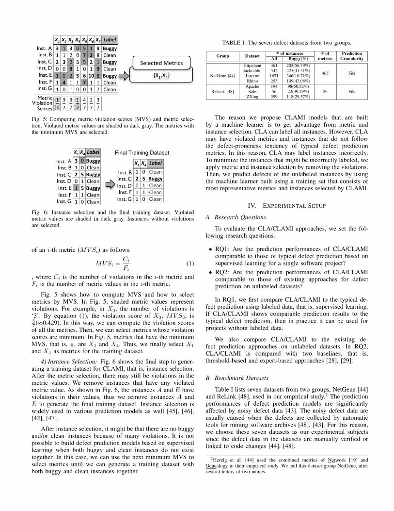
Fig. 5 shows how to compute MVS and how to selectmetrics by MVS. In Fig. 5, shaded metric values representviolations. For example, in X3, the number of violations is‘3’. By equation (1), the violation score of X3, MV S3, is37 (≈0.429). In this way, we can compute the violation scoresof all the metrics. Then, we can select metrics whose violationscores are minimum. In Fig. 5, metrics that have the minimumMVS, that is, 1

7 , are X1 and X4. Thus, we finally select X1

and X4 as metrics for the training dataset.

4) Instance Selection: Fig. 6 shows the final step to gener-ating a training dataset for CLAMI, that is, instance selection.After the metric selection, there may still be violations in themetric values. We remove instances that have any violatedmetric value. As shown in Fig. 6, the instances A and E haveviolations in their values, thus we remove instances A andE to generate the final training dataset. Instance selection iswidely used in various prediction models as well [45], [46],[42], [47].

After instance selection, it might be that there are no buggyand/or clean instances because of many violations. It is notpossible to build defect prediction models based on supervisedlearning when both buggy and clean instances do not existtogether. In this case, we can use the next minimum MVS toselect metrics until we can generate a training dataset withboth buggy and clean instances together.

TABLE I: The seven defect datasets from two groups.

Group Dataset # of instances # ofmetrics

PredictionGranularityAll Buggy(%)

NetGene [44]

Httpclient 361 205(56.79%)

465 FileJackrabbit 542 225(41.51%)Lucene 1671 346(10.71%)Rhino 253 109(43.08%)

ReLink [48]Apache 194 98(50.52%)

26 FileSafe 56 22(39.29%)ZXing 399 118(29.57%)

The reason we propose CLAMI models that are builtby a machine learner is to get advantage from metric andinstance selection. CLA can label all instances. However, CLAmay have violated metrics and instances that do not followthe defect-proneness tendency of typical defect predictionmetrics. In this reason, CLA may label instances incorrectly.To minimize the instances that might be incorrectly labeled, weapply metric and instance selection by removing the violations.Then, we predict defects of the unlabeled instances by usingthe machine learner built using a training set that consists ofmost representative metrics and instances selected by CLAMI.

IV. EXPERIMENTAL SETUP

A. Research Questions

To evaluate the CLA/CLAMI approaches, we set the fol-lowing research questions.

• RQ1: Are the prediction performances of CLA/CLAMIcomparable to those of typical defect prediction based onsupervised learning for a single software project?

• RQ2: Are the prediction performances of CLA/CLAMIcomparable to those of existing approaches for defectprediction on unlabeled datasets?

In RQ1, we first compare CLA/CLAMI to the typical de-fect prediction using labeled data, that is, supervised learning.If CLA/CLAMI shows comparable prediction results to thetypical defect prediction, then in practice it can be used forprojects without labeled data.

We also compare CLA/CLAMI to the existing de-fect prediction approaches on unlabeled datasets. In RQ2,CLA/CLAMI is compared with two baselines, that is,threshold-based and expert-based approaches [28], [29].

B. Benchmark Datasets

Table I lists seven datasets from two groups, NetGene [44]and ReLink [48], used in our empirical study.2 The predictionperformances of defect prediction models are significantlyaffected by noisy defect data [43]. The noisy defect data areusually caused when the defects are collected by automatictools for mining software archives [48], [43]. For this reason,we choose these seven datasets as our experimental subjectssince the defect data in the datasets are manually verified orlinked to code changes [44], [48].

2Herzig et al. [44] used the combined metrics of Network [19] andGenealogy in their empirical study. We call this dataset group NetGene, afterseveral letters of two names.

Experimental Settings (RQ1) - Supervised learning model -

74

Test set (50%)

Training set (50%)

Supervised Model

(Baseline1)

Training

Predict

CLA/ CLAMI Model

Training

Predict

Predict Threshold- Based

(Baseline2)

Expert- Based

(Baseline3)

Training

Predict

Training

Predict

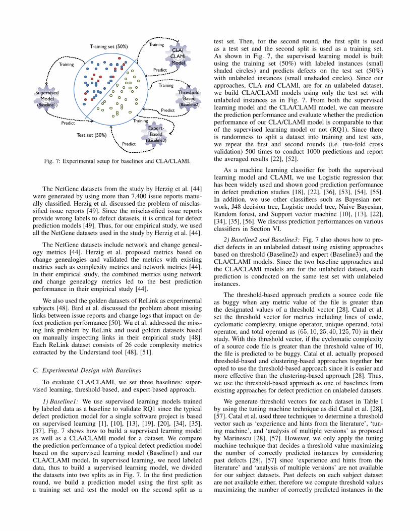
Fig. 7: Experimental setup for baselines and CLA/CLAMI.

The NetGene datasets from the study by Herzig et al. [44]were generated by using more than 7,400 issue reports manu-ally classified. Herzig et al. discussed the problem of misclas-sified issue reports [49]. Since the misclassified issue reportsprovide wrong labels to defect datasets, it is critical for defectprediction models [49]. Thus, for our empirical study, we usedall the NetGene datasets used in the study by Herzig et al. [44].

The NetGene datasets include network and change geneal-ogy metrics [44]. Herzig et al. proposed metrics based onchange genealogies and validated the metrics with existingmetrics such as complexity metrics and network metrics [44].In their empirical study, the combined metrics using networkand change genealogy metrics led to the best predictionperformance in their empirical study [44].

We also used the golden datasets of ReLink as experimentalsubjects [48]. Bird et al. discussed the problem about missinglinks between issue reports and change logs that impact on de-fect prediction performance [50]. Wu et al. addressed the miss-ing link problem by ReLink and used golden datasets basedon manually inspecting links in their empirical study [48].Each ReLink dataset consists of 26 code complexity metricsextracted by the Understand tool [48], [51].

C. Experimental Design with Baselines

To evaluate CLA/CLAMI, we set three baselines: super-vised learning, threshold-based, and expert-based approach.

1) Baseline1: We use supervised learning models trainedby labeled data as a baseline to validate RQ1 since the typicaldefect prediction model for a single software project is basedon supervised learning [1], [10], [13], [19], [20], [34], [35],[37]. Fig. 7 shows how to build a supervised learning modelas well as a CLA/CLAMI model for a dataset. We comparethe prediction performance of a typical defect prediction modelbased on the supervised learning model (Baseline1) and ourCLA/CLAMI model. In supervised learning, we need labeleddata, thus to build a supervised learning model, we dividedthe datasets into two splits as in Fig. 7. In the first predictionround, we build a prediction model using the first split asa training set and test the model on the second split as a

test set. Then, for the second round, the first split is usedas a test set and the second split is used as a training set.As shown in Fig. 7, the supervised learning model is builtusing the training set (50%) with labeled instances (smallshaded circles) and predicts defects on the test set (50%)with unlabeled instances (small unshaded circles). Since ourapproaches, CLA and CLAMI, are for an unlabeled dataset,we build CLA/CLAMI models using only the test set withunlabeled instances as in Fig. 7. From both the supervisedlearning model and the CLA/CLAMI model, we can measurethe prediction performance and evaluate whether the predictionperformance of our CLA/CLAMI model is comparable to thatof the supervised learning model or not (RQ1). Since thereis randomness to split a dataset into training and test sets,we repeat the first and second rounds (i.e. two-fold crossvalidation) 500 times to conduct 1000 predictions and reportthe averaged results [22], [52].

As a machine learning classifier for both the supervisedlearning model and CLAMI, we use Logistic regression thathas been widely used and shown good prediction performancein defect prediction studies [18], [22], [36], [53], [54], [55].In addition, we use other classifiers such as Bayesian net-work, J48 decision tree, Logistic model tree, Naive Bayesian,Random forest, and Support vector machine [10], [13], [22],[34], [35], [56]. We discuss prediction performances on variousclassifiers in Section VI.

2) Baseline2 and Baseline3: Fig. 7 also shows how to pre-dict defects in an unlabeled dataset using existing approachesbased on threshold (Baseline2) and expert (Baseline3) and theCLA/CLAMI models. Since the two baseline approaches andthe CLA/CLAMI models are for the unlabeled dataset, eachprediction is conducted on the same test set with unlabeledinstances.

The threshold-based approach predicts a source code fileas buggy when any metric value of the file is greater thanthe designated values of a threshold vector [28]. Catal et al.set the threshold vector for metrics including lines of code,cyclomatic complexity, unique operator, unique operand, totaloperator, and total operand as (65, 10, 25, 40, 125, 70) in theirstudy. With this threshold vector, if the cyclomatic complexityof a source code file is greater than the threshold value of 10,the file is predicted to be buggy. Catal et al. actually proposedthreshold-based and clustering-based approaches together butopted to use the threshold-based approach since it is easier andmore effective than the clustering-based approach [28]. Thus,we use the threshold-based approach as one of baselines fromexisting approaches for defect prediction on unlabeled datasets.

We generate threshold vectors for each dataset in Table Iby using the tuning machine technique as did Catal et al. [28],[57]. Catal et al. used three techniques to determine a thresholdvector such as ‘experience and hints from the literature’, ‘tun-ing machine’, and ‘analysis of multiple versions’ as proposedby Marinescu [28], [57]. However, we only apply the tuningmachine technique that decides a threshold value maximizingthe number of correctly predicted instances by consideringpast defects [28], [57] since ‘experience and hints from theliterature’ and ‘analysis of multiple versions’ are not availablefor our subject datasets. Past defects on each subject datasetare not available either, therefore we compute threshold valuesmaximizing the number of correctly predicted instances in the

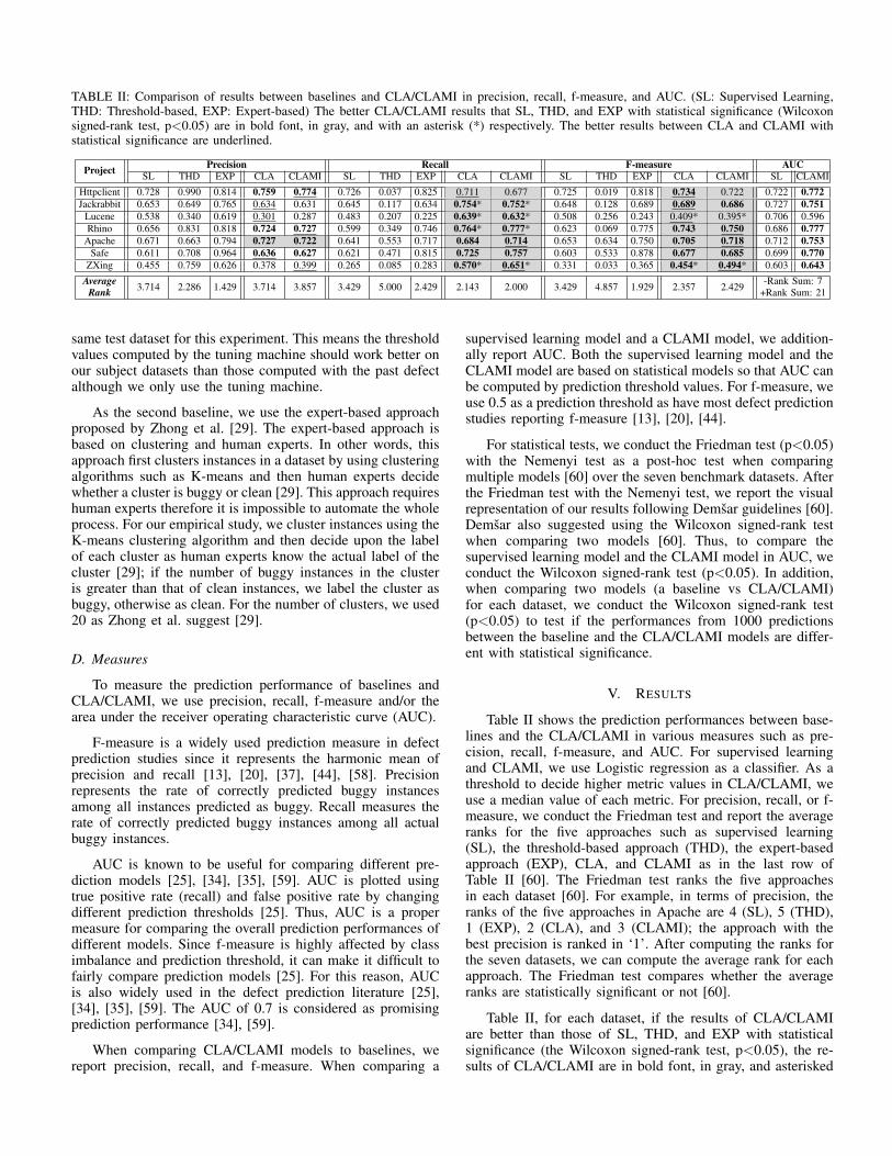
TABLE II: Comparison of results between baselines and CLA/CLAMI in precision, recall, f-measure, and AUC. (SL: Supervised Learning,THD: Threshold-based, EXP: Expert-based) The better CLA/CLAMI results that SL, THD, and EXP with statistical significance (Wilcoxonsigned-rank test, p<0.05) are in bold font, in gray, and with an asterisk (*) respectively. The better results between CLA and CLAMI withstatistical significance are underlined.

Project Precision Recall F-measure AUCSL THD EXP CLA CLAMI SL THD EXP CLA CLAMI SL THD EXP CLA CLAMI SL CLAMI

Httpclient 0.728 0.990 0.814 0.759 0.774 0.726 0.037 0.825 0.711 0.677 0.725 0.019 0.818 0.734 0.722 0.722 0.772Jackrabbit 0.653 0.649 0.765 0.634 0.631 0.645 0.117 0.634 0.754* 0.752* 0.648 0.128 0.689 0.689 0.686 0.727 0.751

Lucene 0.538 0.340 0.619 0.301 0.287 0.483 0.207 0.225 0.639* 0.632* 0.508 0.256 0.243 0.409* 0.395* 0.706 0.596Rhino 0.656 0.831 0.818 0.724 0.727 0.599 0.349 0.746 0.764* 0.777* 0.623 0.069 0.775 0.743 0.750 0.686 0.777

Apache 0.671 0.663 0.794 0.727 0.722 0.641 0.553 0.717 0.684 0.714 0.653 0.634 0.750 0.705 0.718 0.712 0.753Safe 0.611 0.708 0.964 0.636 0.627 0.621 0.471 0.815 0.725 0.757 0.603 0.533 0.878 0.677 0.685 0.699 0.770

ZXing 0.455 0.759 0.626 0.378 0.399 0.265 0.085 0.283 0.570* 0.651* 0.331 0.033 0.365 0.454* 0.494* 0.603 0.643Average

Rank 3.714 2.286 1.429 3.714 3.857 3.429 5.000 2.429 2.143 2.000 3.429 4.857 1.929 2.357 2.429 -Rank Sum: 7+Rank Sum: 21

same test dataset for this experiment. This means the thresholdvalues computed by the tuning machine should work better onour subject datasets than those computed with the past defectalthough we only use the tuning machine.

As the second baseline, we use the expert-based approachproposed by Zhong et al. [29]. The expert-based approach isbased on clustering and human experts. In other words, thisapproach first clusters instances in a dataset by using clusteringalgorithms such as K-means and then human experts decidewhether a cluster is buggy or clean [29]. This approach requireshuman experts therefore it is impossible to automate the wholeprocess. For our empirical study, we cluster instances using theK-means clustering algorithm and then decide upon the labelof each cluster as human experts know the actual label of thecluster [29]; if the number of buggy instances in the clusteris greater than that of clean instances, we label the cluster asbuggy, otherwise as clean. For the number of clusters, we used20 as Zhong et al. suggest [29].

D. Measures

To measure the prediction performance of baselines andCLA/CLAMI, we use precision, recall, f-measure and/or thearea under the receiver operating characteristic curve (AUC).

F-measure is a widely used prediction measure in defectprediction studies since it represents the harmonic mean ofprecision and recall [13], [20], [37], [44], [58]. Precisionrepresents the rate of correctly predicted buggy instancesamong all instances predicted as buggy. Recall measures therate of correctly predicted buggy instances among all actualbuggy instances.

AUC is known to be useful for comparing different pre-diction models [25], [34], [35], [59]. AUC is plotted usingtrue positive rate (recall) and false positive rate by changingdifferent prediction thresholds [25]. Thus, AUC is a propermeasure for comparing the overall prediction performances ofdifferent models. Since f-measure is highly affected by classimbalance and prediction threshold, it can make it difficult tofairly compare prediction models [25]. For this reason, AUCis also widely used in the defect prediction literature [25],[34], [35], [59]. The AUC of 0.7 is considered as promisingprediction performance [34], [59].

When comparing CLA/CLAMI models to baselines, wereport precision, recall, and f-measure. When comparing a

supervised learning model and a CLAMI model, we addition-ally report AUC. Both the supervised learning model and theCLAMI model are based on statistical models so that AUC canbe computed by prediction threshold values. For f-measure, weuse 0.5 as a prediction threshold as have most defect predictionstudies reporting f-measure [13], [20], [44].

For statistical tests, we conduct the Friedman test (p<0.05)with the Nemenyi test as a post-hoc test when comparingmultiple models [60] over the seven benchmark datasets. Afterthe Friedman test with the Nemenyi test, we report the visualrepresentation of our results following Demsar guidelines [60].Demsar also suggested using the Wilcoxon signed-rank testwhen comparing two models [60]. Thus, to compare thesupervised learning model and the CLAMI model in AUC, weconduct the Wilcoxon signed-rank test (p<0.05). In addition,when comparing two models (a baseline vs CLA/CLAMI)for each dataset, we conduct the Wilcoxon signed-rank test(p<0.05) to test if the performances from 1000 predictionsbetween the baseline and the CLA/CLAMI models are differ-ent with statistical significance.

V. RESULTS

Table II shows the prediction performances between base-lines and the CLA/CLAMI in various measures such as pre-cision, recall, f-measure, and AUC. For supervised learningand CLAMI, we use Logistic regression as a classifier. As athreshold to decide higher metric values in CLA/CLAMI, weuse a median value of each metric. For precision, recall, or f-measure, we conduct the Friedman test and report the averageranks for the five approaches such as supervised learning(SL), the threshold-based approach (THD), the expert-basedapproach (EXP), CLA, and CLAMI as in the last row ofTable II [60]. The Friedman test ranks the five approachesin each dataset [60]. For example, in terms of precision, theranks of the five approaches in Apache are 4 (SL), 5 (THD),1 (EXP), 2 (CLA), and 3 (CLAMI); the approach with thebest precision is ranked in ‘1’. After computing the ranks forthe seven datasets, we can compute the average rank for eachapproach. The Friedman test compares whether the averageranks are statistically significant or not [60].

Table II, for each dataset, if the results of CLA/CLAMIare better than those of SL, THD, and EXP with statisticalsignificance (the Wilcoxon signed-rank test, p<0.05), the re-sults of CLA/CLAMI are in bold font, in gray, and asterisked

1 2 5 4 3

THD CLA CLAMI EXP

SL

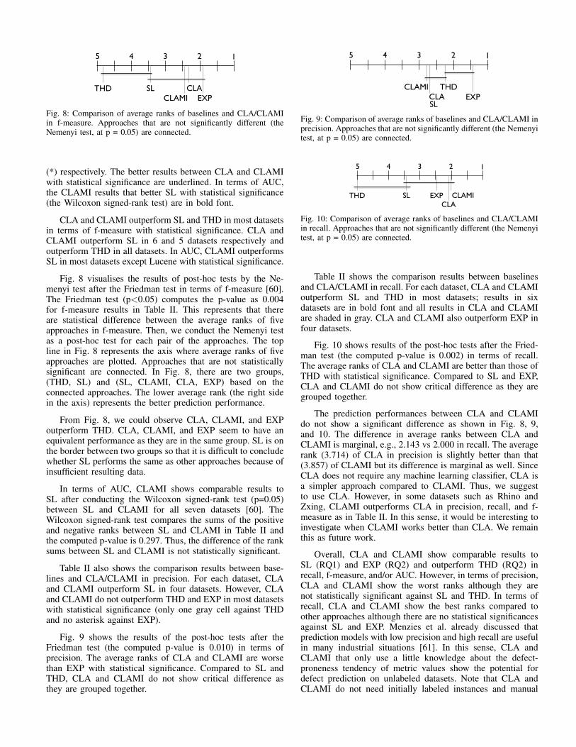
Fig. 8: Comparison of average ranks of baselines and CLA/CLAMIin f-measure. Approaches that are not significantly different (theNemenyi test, at p = 0.05) are connected.

(*) respectively. The better results between CLA and CLAMIwith statistical significance are underlined. In terms of AUC,the CLAMI results that better SL with statistical significance(the Wilcoxon signed-rank test) are in bold font.

CLA and CLAMI outperform SL and THD in most datasetsin terms of f-measure with statistical significance. CLA andCLAMI outperform SL in 6 and 5 datasets respectively andoutperform THD in all datasets. In AUC, CLAMI outperformsSL in most datasets except Lucene with statistical significance.

Fig. 8 visualises the results of post-hoc tests by the Ne-menyi test after the Friedman test in terms of f-measure [60].The Friedman test (p<0.05) computes the p-value as 0.004for f-measure results in Table II. This represents that thereare statistical difference between the average ranks of fiveapproaches in f-measure. Then, we conduct the Nemenyi testas a post-hoc test for each pair of the approaches. The topline in Fig. 8 represents the axis where average ranks of fiveapproaches are plotted. Approaches that are not statisticallysignificant are connected. In Fig. 8, there are two groups,(THD, SL) and (SL, CLAMI, CLA, EXP) based on theconnected approaches. The lower average rank (the right sidein the axis) represents the better prediction performance.

From Fig. 8, we could observe CLA, CLAMI, and EXPoutperform THD. CLA, CLAMI, and EXP seem to have anequivalent performance as they are in the same group. SL is onthe border between two groups so that it is difficult to concludewhether SL performs the same as other approaches because ofinsufficient resulting data.

In terms of AUC, CLAMI shows comparable results toSL after conducting the Wilcoxon signed-rank test (p=0.05)between SL and CLAMI for all seven datasets [60]. TheWilcoxon signed-rank test compares the sums of the positiveand negative ranks between SL and CLAMI in Table II andthe computed p-value is 0.297. Thus, the difference of the ranksums between SL and CLAMI is not statistically significant.

Table II also shows the comparison results between base-lines and CLA/CLAMI in precision. For each dataset, CLAand CLAMI outperform SL in four datasets. However, CLAand CLAMI do not outperform THD and EXP in most datasetswith statistical significance (only one gray cell against THDand no asterisk against EXP).

Fig. 9 shows the results of the post-hoc tests after theFriedman test (the computed p-value is 0.010) in terms ofprecision. The average ranks of CLA and CLAMI are worsethan EXP with statistical significance. Compared to SL andTHD, CLA and CLAMI do not show critical difference asthey are grouped together.

1 2 5 4 3

THD CLA

CLAMI EXP

SL

Fig. 9: Comparison of average ranks of baselines and CLA/CLAMI inprecision. Approaches that are not significantly different (the Nemenyitest, at p = 0.05) are connected.

1 2 5 4 3

THD CLA

CLAMI EXP SL

Fig. 10: Comparison of average ranks of baselines and CLA/CLAMIin recall. Approaches that are not significantly different (the Nemenyitest, at p = 0.05) are connected.

Table II shows the comparison results between baselinesand CLA/CLAMI in recall. For each dataset, CLA and CLAMIoutperform SL and THD in most datasets; results in sixdatasets are in bold font and all results in CLA and CLAMIare shaded in gray. CLA and CLAMI also outperform EXP infour datasets.

Fig. 10 shows results of the post-hoc tests after the Fried-man test (the computed p-value is 0.002) in terms of recall.The average ranks of CLA and CLAMI are better than those ofTHD with statistical significance. Compared to SL and EXP,CLA and CLAMI do not show critical difference as they aregrouped together.

The prediction performances between CLA and CLAMIdo not show a significant difference as shown in Fig. 8, 9,and 10. The difference in average ranks between CLA andCLAMI is marginal, e.g., 2.143 vs 2.000 in recall. The averagerank (3.714) of CLA in precision is slightly better than that(3.857) of CLAMI but its difference is marginal as well. SinceCLA does not require any machine learning classifier, CLA isa simpler approach compared to CLAMI. Thus, we suggestto use CLA. However, in some datasets such as Rhino andZxing, CLAMI outperforms CLA in precision, recall, and f-measure as in Table II. In this sense, it would be interesting toinvestigate when CLAMI works better than CLA. We remainthis as future work.

Overall, CLA and CLAMI show comparable results toSL (RQ1) and EXP (RQ2) and outperform THD (RQ2) inrecall, f-measure, and/or AUC. However, in terms of precision,CLA and CLAMI show the worst ranks although they arenot statistically significant against SL and THD. In terms ofrecall, CLA and CLAMI show the best ranks compared toother approaches although there are no statistical significancesagainst SL and EXP. Menzies et al. already discussed thatprediction models with low precision and high recall are usefulin many industrial situations [61]. In this sense, CLA andCLAMI that only use a little knowledge about the defect-proneness tendency of metric values show the potential fordefect prediction on unlabeled datasets. Note that CLA andCLAMI do not need initially labeled instances and manual

1 2 7 6 5 4 3

LMT NB LR BN

RF J48 SVM

Fig. 11: Comparison of all classifiers against each other in AUC.Approaches that are not significantly different (the Nemenyi test, atp = 0.05) are connected.

1 2 7 6 5 4 3

LMT NB LR

BN RF J48 SVM

Fig. 12: Comparison of all classifiers against each other in f-measure.Approaches that are not significantly different (the Nemenyi test, atp = 0.05) are connected.

effort but achieve comparable prediction performances to mostbaselines in terms of recall, f-measure, and AUC.

VI. DISCUSSION

A. Performance on Various Classifiers

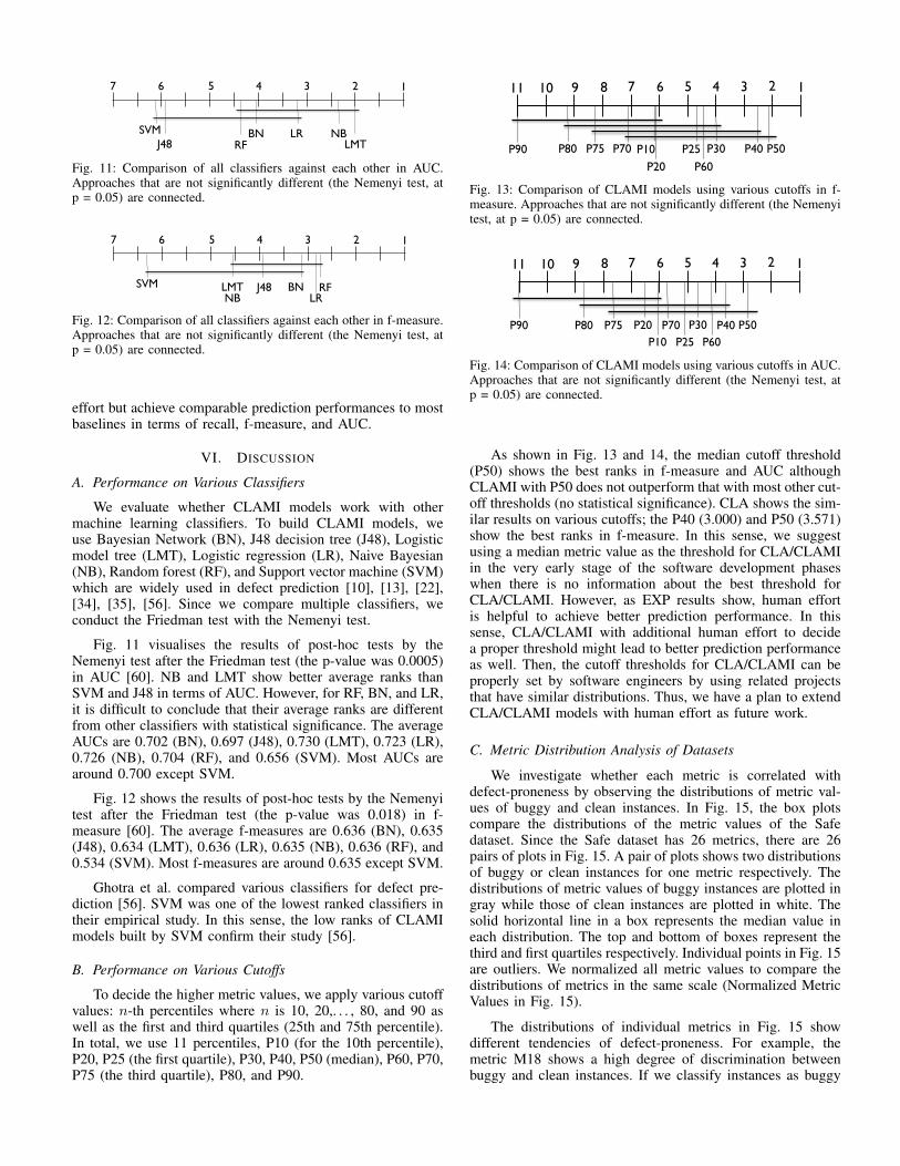
We evaluate whether CLAMI models work with othermachine learning classifiers. To build CLAMI models, weuse Bayesian Network (BN), J48 decision tree (J48), Logisticmodel tree (LMT), Logistic regression (LR), Naive Bayesian(NB), Random forest (RF), and Support vector machine (SVM)which are widely used in defect prediction [10], [13], [22],[34], [35], [56]. Since we compare multiple classifiers, weconduct the Friedman test with the Nemenyi test.

Fig. 11 visualises the results of post-hoc tests by theNemenyi test after the Friedman test (the p-value was 0.0005)in AUC [60]. NB and LMT show better average ranks thanSVM and J48 in terms of AUC. However, for RF, BN, and LR,it is difficult to conclude that their average ranks are differentfrom other classifiers with statistical significance. The averageAUCs are 0.702 (BN), 0.697 (J48), 0.730 (LMT), 0.723 (LR),0.726 (NB), 0.704 (RF), and 0.656 (SVM). Most AUCs arearound 0.700 except SVM.

Fig. 12 shows the results of post-hoc tests by the Nemenyitest after the Friedman test (the p-value was 0.018) in f-measure [60]. The average f-measures are 0.636 (BN), 0.635(J48), 0.634 (LMT), 0.636 (LR), 0.635 (NB), 0.636 (RF), and0.534 (SVM). Most f-measures are around 0.635 except SVM.

Ghotra et al. compared various classifiers for defect pre-diction [56]. SVM was one of the lowest ranked classifiers intheir empirical study. In this sense, the low ranks of CLAMImodels built by SVM confirm their study [56].

B. Performance on Various Cutoffs

To decide the higher metric values, we apply various cutoffvalues: n-th percentiles where n is 10, 20,. . . , 80, and 90 aswell as the first and third quartiles (25th and 75th percentile).In total, we use 11 percentiles, P10 (for the 10th percentile),P20, P25 (the first quartile), P30, P40, P50 (median), P60, P70,P75 (the third quartile), P80, and P90.

1 2 7 6 5 4 3

P25 P70 P80 P50 P60

P30 P20

8 9 10 11

P90 P75 P40 P10

Fig. 13: Comparison of CLAMI models using various cutoffs in f-measure. Approaches that are not significantly different (the Nemenyitest, at p = 0.05) are connected.

1 2 7 6 5 4 3

P25 P70 P80 P50

P60 P30 P20

8 9 10 11

P90 P75 P40 P10

Fig. 14: Comparison of CLAMI models using various cutoffs in AUC.Approaches that are not significantly different (the Nemenyi test, atp = 0.05) are connected.

As shown in Fig. 13 and 14, the median cutoff threshold(P50) shows the best ranks in f-measure and AUC althoughCLAMI with P50 does not outperform that with most other cut-off thresholds (no statistical significance). CLA shows the sim-ilar results on various cutoffs; the P40 (3.000) and P50 (3.571)show the best ranks in f-measure. In this sense, we suggestusing a median metric value as the threshold for CLA/CLAMIin the very early stage of the software development phaseswhen there is no information about the best threshold forCLA/CLAMI. However, as EXP results show, human effortis helpful to achieve better prediction performance. In thissense, CLA/CLAMI with additional human effort to decidea proper threshold might lead to better prediction performanceas well. Then, the cutoff thresholds for CLA/CLAMI can beproperly set by software engineers by using related projectsthat have similar distributions. Thus, we have a plan to extendCLA/CLAMI models with human effort as future work.

C. Metric Distribution Analysis of Datasets

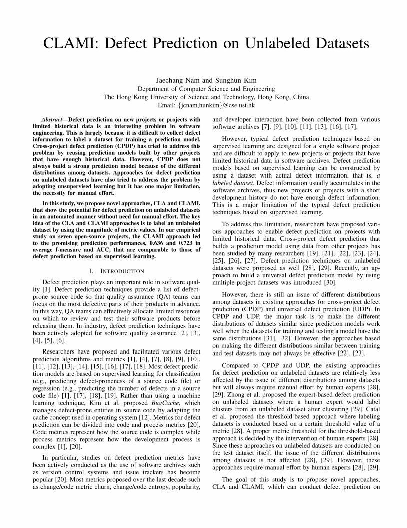
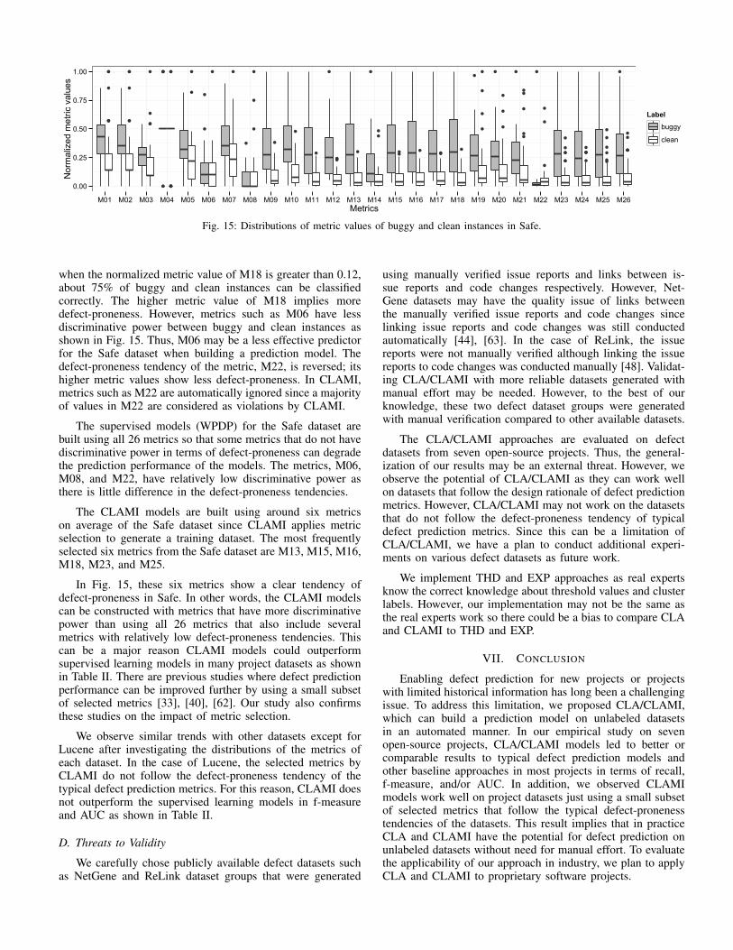
We investigate whether each metric is correlated withdefect-proneness by observing the distributions of metric val-ues of buggy and clean instances. In Fig. 15, the box plotscompare the distributions of the metric values of the Safedataset. Since the Safe dataset has 26 metrics, there are 26pairs of plots in Fig. 15. A pair of plots shows two distributionsof buggy or clean instances for one metric respectively. Thedistributions of metric values of buggy instances are plotted ingray while those of clean instances are plotted in white. Thesolid horizontal line in a box represents the median value ineach distribution. The top and bottom of boxes represent thethird and first quartiles respectively. Individual points in Fig. 15are outliers. We normalized all metric values to compare thedistributions of metrics in the same scale (Normalized MetricValues in Fig. 15).

The distributions of individual metrics in Fig. 15 showdifferent tendencies of defect-proneness. For example, themetric M18 shows a high degree of discrimination betweenbuggy and clean instances. If we classify instances as buggy

0.00

0.25

0.50

0.75

1.00

M01 M02 M03 M04 M05 M06 M07 M08 M09 M10 M11 M12 M13 M14 M15 M16 M17 M18 M19 M20 M21 M22 M23 M24 M25 M26Metrics

Nor

mal

ized

met

ric v

alue

s

Labelbuggy

clean

Fig. 15: Distributions of metric values of buggy and clean instances in Safe.

when the normalized metric value of M18 is greater than 0.12,about 75% of buggy and clean instances can be classifiedcorrectly. The higher metric value of M18 implies moredefect-proneness. However, metrics such as M06 have lessdiscriminative power between buggy and clean instances asshown in Fig. 15. Thus, M06 may be a less effective predictorfor the Safe dataset when building a prediction model. Thedefect-proneness tendency of the metric, M22, is reversed; itshigher metric values show less defect-proneness. In CLAMI,metrics such as M22 are automatically ignored since a majorityof values in M22 are considered as violations by CLAMI.

The supervised models (WPDP) for the Safe dataset arebuilt using all 26 metrics so that some metrics that do not havediscriminative power in terms of defect-proneness can degradethe prediction performance of the models. The metrics, M06,M08, and M22, have relatively low discriminative power asthere is little difference in the defect-proneness tendencies.

The CLAMI models are built using around six metricson average of the Safe dataset since CLAMI applies metricselection to generate a training dataset. The most frequentlyselected six metrics from the Safe dataset are M13, M15, M16,M18, M23, and M25.

In Fig. 15, these six metrics show a clear tendency ofdefect-proneness in Safe. In other words, the CLAMI modelscan be constructed with metrics that have more discriminativepower than using all 26 metrics that also include severalmetrics with relatively low defect-proneness tendencies. Thiscan be a major reason CLAMI models could outperformsupervised learning models in many project datasets as shownin Table II. There are previous studies where defect predictionperformance can be improved further by using a small subsetof selected metrics [33], [40], [62]. Our study also confirmsthese studies on the impact of metric selection.

We observe similar trends with other datasets except forLucene after investigating the distributions of the metrics ofeach dataset. In the case of Lucene, the selected metrics byCLAMI do not follow the defect-proneness tendency of thetypical defect prediction metrics. For this reason, CLAMI doesnot outperform the supervised learning models in f-measureand AUC as shown in Table II.

D. Threats to Validity

We carefully chose publicly available defect datasets suchas NetGene and ReLink dataset groups that were generated

using manually verified issue reports and links between is-sue reports and code changes respectively. However, Net-Gene datasets may have the quality issue of links betweenthe manually verified issue reports and code changes sincelinking issue reports and code changes was still conductedautomatically [44], [63]. In the case of ReLink, the issuereports were not manually verified although linking the issuereports to code changes was conducted manually [48]. Validat-ing CLA/CLAMI with more reliable datasets generated withmanual effort may be needed. However, to the best of ourknowledge, these two defect dataset groups were generatedwith manual verification compared to other available datasets.

The CLA/CLAMI approaches are evaluated on defectdatasets from seven open-source projects. Thus, the general-ization of our results may be an external threat. However, weobserve the potential of CLA/CLAMI as they can work wellon datasets that follow the design rationale of defect predictionmetrics. However, CLA/CLAMI may not work on the datasetsthat do not follow the defect-proneness tendency of typicaldefect prediction metrics. Since this can be a limitation ofCLA/CLAMI, we have a plan to conduct additional experi-ments on various defect datasets as future work.

We implement THD and EXP approaches as real expertsknow the correct knowledge about threshold values and clusterlabels. However, our implementation may not be the same asthe real experts work so there could be a bias to compare CLAand CLAMI to THD and EXP.

VII. CONCLUSION

Enabling defect prediction for new projects or projectswith limited historical information has long been a challengingissue. To address this limitation, we proposed CLA/CLAMI,which can build a prediction model on unlabeled datasetsin an automated manner. In our empirical study on sevenopen-source projects, CLA/CLAMI models led to better orcomparable results to typical defect prediction models andother baseline approaches in most projects in terms of recall,f-measure, and/or AUC. In addition, we observed CLAMImodels work well on project datasets just using a small subsetof selected metrics that follow the typical defect-pronenesstendencies of the datasets. This result implies that in practiceCLA and CLAMI have the potential for defect prediction onunlabeled datasets without need for manual effort. To evaluatethe applicability of our approach in industry, we plan to applyCLA and CLAMI to proprietary software projects.

REFERENCES

[1] T. Menzies, J. Greenwald, and A. Frank, “Data mining static codeattributes to learn defect predictors,” IEEE Trans. Softw. Eng., vol. 33,pp. 2–13, January 2007.

[2] E. Engstrom, P. Runeson, and G. Wikstrand, “An empirical evaluationof regression testing based on fix-cache recommendations,” in SoftwareTesting, Verification and Validation (ICST), 2010 Third InternationalConference on, April 2010, pp. 75–78.

[3] N. Nagappan, T. Ball, and A. Zeller, “Mining metrics to predictcomponent failures,” in Proceedings of the 28th InternationalConference on Software Engineering, ser. ICSE ’06. NewYork, NY, USA: ACM, 2006, pp. 452–461. [Online]. Available:http://doi.acm.org/10.1145/1134285.1134349

[4] N. Ohlsson and H. Alberg, “Predicting fault-prone software modulesin telephone switches,” Software Engineering, IEEE Transactions on,vol. 22, no. 12, pp. 886–894, Dec 1996.

[5] T. Ostrand, E. Weyuker, and R. Bell, “Predicting the location andnumber of faults in large software systems,” Software Engineering,IEEE Transactions on, vol. 31, no. 4, pp. 340–355, April 2005.

[6] P. Tomaszewski, H. Grahn, and L. Lundberg, “A method for an accurateearly prediction of faults in modified classes,” in Software Maintenance,2006. ICSM ’06. 22nd IEEE International Conference on, Sept 2006,pp. 487–496.

[7] A. Bacchelli, M. D’Ambros, and M. Lanza, “Are popular classes moredefect prone?” in Proceedings of the 13th International Conferenceon Fundamental Approaches to Software Engineering, ser. FASE’10.Berlin, Heidelberg: Springer-Verlag, 2010, pp. 59–73.

[8] V. R. Basili, L. C. Briand, and W. L. Melo, “A validation of object-oriented design metrics as quality indicators,” IEEE Trans. Softw. Eng.,vol. 22, pp. 751–761, October 1996.

[9] C. Bird, N. Nagappan, B. Murphy, H. Gall, and P. Devanbu, “Don’ttouch my code!: Examining the effects of ownership on softwarequality,” in Proceedings of the 19th ACM SIGSOFT Symposium and the13th European Conference on Foundations of Software Engineering,ser. ESEC/FSE ’11. New York, NY, USA: ACM, 2011, pp. 4–14.[Online]. Available: http://doi.acm.org/10.1145/2025113.2025119

[10] M. D’Ambros, M. Lanza, and R. Robbes, “Evaluating defect predictionapproaches: a benchmark and an extensive comparison,” EmpiricalSoftware Engineering, vol. 17, no. 4-5, pp. 531–577, 2012.

[11] A. E. Hassan, “Predicting faults using the complexity of code changes,”in Proceedings of the 31st International Conference on Software Engi-neering, ser. ICSE ’09, 2009, pp. 78–88.

[12] S. Kim, T. Zimmermann, E. J. Whitehead Jr., and A. Zeller, “Predictingfaults from cached history,” in Proceedings of the 29th internationalconference on Software Engineering, ser. ICSE ’07, 2007, pp. 489–498.

[13] T. Lee, J. Nam, D. Han, S. Kim, and I. P. Hoh, “Micro interaction met-rics for defect prediction,” in Proceedings of the 16th ACM SIGSOFTInternational Symposium on Foundations of software engineering, 2011.

[14] M. Li, H. Zhang, R. Wu, and Z.-H. Zhou, “Sample-based softwaredefect prediction with active and semi-supervised learning,” AutomatedSoftware Engineering, vol. 19, no. 2, pp. 201–230, 2012. [Online].Available: http://dx.doi.org/10.1007/s10515-011-0092-1

[15] H. Lu and B. Cukic, “An adaptive approach with active learningin software fault prediction,” in Proceedings of the 8th InternationalConference on Predictive Models in Software Engineering, ser.PROMISE ’12. New York, NY, USA: ACM, 2012, pp. 79–88.[Online]. Available: http://doi.acm.org/10.1145/2365324.2365335

[16] R. Moser, W. Pedrycz, and G. Succi, “A comparative analysis ofthe efficiency of change metrics and static code attributes for defectprediction,” in Proceedings of the 30th international conference onSoftware engineering, ser. ICSE ’08, 2008, pp. 181–190.

[17] N. Nagappan and T. Ball, “Use of relative code churn measures topredict system defect density,” in Proceedings of the 27th internationalconference on Software engineering, ser. ICSE ’05, 2005, pp. 284–292.

[18] T. Zimmermann, N. Nagappan, H. Gall, E. Giger, and B. Murphy,“Cross-project defect prediction: a large scale experiment on data vs.domain vs. process,” in Proceedings of the the 7th joint meeting ofthe European software engineering conference and the ACM SIGSOFTsymposium on The foundations of software engineering. New York,NY, USA: ACM, 2009, pp. 91–100.

[19] T. Zimmermann and N. Nagappan, “Predicting defects using networkanalysis on dependency graphs,” in Proceedings of the 30th interna-tional conference on Software engineering, 2008, pp. 531–540.

[20] F. Rahman and P. Devanbu, “How, and why, process metrics are better,”in Proceedings of the 2013 International Conference on SoftwareEngineering. Piscataway, NJ, USA: IEEE Press, 2013, pp. 432–441.

[21] Y. Ma, G. Luo, X. Zeng, and A. Chen, “Transfer learning for cross-company software defect prediction,” Inf. Softw. Technol., vol. 54, no. 3,pp. 248–256, Mar. 2012.

[22] J. Nam, S. J. Pan, and S. Kim, “Transfer defect learning,” in Proceed-ings of the 2013 International Conference on Software Engineering.Piscataway, NJ, USA: IEEE Press, 2013, pp. 382–391.

[23] B. Turhan, T. Menzies, A. B. Bener, and J. Di Stefano, “On the relativevalue of cross-company and within-company data for defect prediction,”Empirical Softw. Eng., vol. 14, pp. 540–578, October 2009.

[24] S. Watanabe, H. Kaiya, and K. Kaijiri, “Adapting a fault predictionmodel to allow inter languagereuse,” in Proceedings of the 4th Interna-tional Workshop on Predictor Models in Software Engineering. NewYork, NY, USA: ACM, 2008, pp. 19–24.

[25] F. Rahman, D. Posnett, and P. Devanbu, “Recalling the ”imprecision”of cross-project defect prediction,” in Proceedings of the ACM SIG-SOFT 20th International Symposium on the Foundations of SoftwareEngineering. New York, NY, USA: ACM, 2012, pp. 61:1–61:11.

[26] G. Canfora, A. De Lucia, M. Di Penta, R. Oliveto, A. Panichella,and S. Panichella, “Multi-objective cross-project defect prediction,”in Software Testing, Verification and Validation, 2013 IEEE SixthInternational Conference on, March 2013, pp. 252–261.

[27] A. Panichella, R. Oliveto, and A. De Lucia, “Cross-project defectprediction models: L’union fait la force,” in Software Maintenance,Reengineering and Reverse Engineering (CSMR-WCRE), 2014 SoftwareEvolution Week - IEEE Conference on, Feb 2014, pp. 164–173.

[28] C. Catal, U. Sevim, and B. Diri, “Clustering and metrics thresholdsbased software fault prediction of unlabeled program modules,” inInformation Technology: New Generations, 2009. ITNG ’09. SixthInternational Conference on, April 2009, pp. 199–204.

[29] S. Zhong, T. Khoshgoftaar, and N. Seliya, “Unsupervised learning forexpert-based software quality estimation,” in High Assurance SystemsEngineering, 2004. Proceedings. Eighth IEEE International Symposiumon, March 2004, pp. 149–155.

[30] F. Zhang, A. Mockus, I. Keivanloo, and Y. Zou, “Towards buildinga universal defect prediction model,” in Proceedings of the 11thWorking Conference on Mining Software Repositories, ser. MSR 2014.New York, NY, USA: ACM, 2014, pp. 182–191. [Online]. Available:http://doi.acm.org/10.1145/2597073.2597078

[31] B. Turhan, “On the dataset shift problem in software engineeringprediction models,” Empirical Software Engineering, vol. 17, no. 1-2,pp. 62–74, 2012. [Online]. Available: http://dx.doi.org/10.1007/s10664-011-9182-8

[32] S. J. Pan and Q. Yang, “A survey on transfer learning,” IEEE Trans. onKnowl. and Data Eng., vol. 22, pp. 1345–1359, October 2010.

[33] S. Shivaji, E. J. Whitehead, R. Akella, and S. Kim, “Reducing featuresto improve code change-based bug prediction,” IEEE Transactions onSoftware Engineering, vol. 39, no. 4, pp. 552–569, 2013.

[34] S. Lessmann, B. Baesens, C. Mues, and S. Pietsch, “Benchmarkingclassification models for software defect prediction: A proposed frame-work and novel findings,” Software Engineering, IEEE Transactions on,vol. 34, no. 4, pp. 485–496, 2008.

[35] Q. Song, Z. Jia, M. Shepperd, S. Ying, and J. Liu, “A general softwaredefect-proneness prediction framework,” Software Engineering, IEEETransactions on, vol. 37, no. 3, pp. 356–370, 2011.

[36] T. Hall, S. Beecham, D. Bowes, D. Gray, and S. Counsell, “A systematicliterature review on fault prediction performance in software engineer-ing,” Software Engineering, IEEE Transactions on, vol. 38, no. 6, pp.1276–1304, Nov 2012.

[37] T. Fukushima, Y. Kamei, S. McIntosh, K. Yamashita, and N. Ubayashi,“An empirical study of just-in-time defect prediction using cross-projectmodels,” in Proceedings of the 11th Working Conference on MiningSoftware Repositories. New York, NY, USA: ACM, 2014, pp. 172–181.

[38] M. Harman, S. Islam, Y. Jia, L. Minku, F. Sarro, and K. Srivisut,“Less is more: Temporal fault predictive performance over multiplehadoop releases,” in Search-Based Software Engineering, ser. LectureNotes in Computer Science, C. Le Goues and S. Yoo, Eds. SpringerInternational Publishing, 2014, vol. 8636, pp. 240–246.

[39] A. L. Blum and P. Langley, “Selection of relevant features andexamples in machine learning,” Artif. Intell., vol. 97, no. 1-2, pp. 245–271, Dec. 1997. [Online]. Available: http://dx.doi.org/10.1016/S0004-3702(97)00063-5

[40] K. Gao, T. M. Khoshgoftaar, H. Wang, and N. Seliya, “Choosingsoftware metrics for defect prediction: An investigation on featureselection techniques,” Softw. Pract. Exper., vol. 41, no. 5, pp. 579–606,Apr. 2011. [Online]. Available: http://dx.doi.org/10.1002/spe.1043

[41] H. Wang, T. M. Khoshgoftaar, and N. Seliya, “How manysoftware metrics should be selected for defect prediction?”in FLAIRS Conference, R. C. Murray and P. M. McCarthy,Eds. AAAI Press, 2011. [Online]. Available: http://dblp.uni-trier.de/db/conf/flairs/flairs2011.htmlWangKS11

[42] E. Kocaguneli, T. Menzies, J. Keung, D. Cok, and R. Madachy, “Activelearning and effort estimation: Finding the essential content of softwareeffort estimation data,” Software Engineering, IEEE Transactions on,vol. 39, no. 8, pp. 1040–1053, 2013.

[43] S. Kim, H. Zhang, R. Wu, and L. Gong, “Dealing with noisein defect prediction,” in Proceedings of the 33rd InternationalConference on Software Engineering, ser. ICSE ’11. NewYork, NY, USA: ACM, 2011, pp. 481–490. [Online]. Available:http://doi.acm.org/10.1145/1985793.1985859

[44] K. Herzig, S. Just, A. Rau, and A. Zeller, “Predicting defects usingchange genealogies,” in Software Reliability Engineering (ISSRE), 2013IEEE 24th International Symposium on, Nov 2013, pp. 118–127.

[45] C.-L. Chang, “Finding prototypes for nearest neighbor classifiers,”Computers, IEEE Transactions on, vol. C-23, no. 11, pp. 1179–1184,Nov 1974.

[46] E. Kocaguneli, T. Menzies, A. Bener, and J. Keung, “Exploiting theessential assumptions of analogy-based effort estimation,” SoftwareEngineering, IEEE Transactions on, vol. 38, no. 2, pp. 425–438, March2012.

[47] Y. F. Li, M. Xie, and T. N. Goh, “A study of project selection andfeature weighting for analogy based software cost estimation,” J. Syst.Softw., vol. 82, no. 2, pp. 241–252, Feb. 2009. [Online]. Available:http://dx.doi.org/10.1016/j.jss.2008.06.001

[48] R. Wu, H. Zhang, S. Kim, and S. Cheung, “Relink: Recovering linksbetween bugs and changes,” in Proceedings of the 16th ACM SIGSOFTInternational Symposium on Foundations of software engineering, 2011.

[49] K. Herzig, S. Just, and A. Zeller, “It’s not a bug, it’s a feature:How misclassification impacts bug prediction,” in Proceedings of the2013 International Conference on Software Engineering, ser. ICSE’13. Piscataway, NJ, USA: IEEE Press, 2013, pp. 392–401. [Online].Available: http://dl.acm.org/citation.cfm?id=2486788.2486840

[50] C. Bird, A. Bachmann, E. Aune, J. Duffy, A. Bernstein, V. Filkov,and P. Devanbu, “Fair and balanced?: Bias in bug-fix datasets,” inProceedings of the the 7th Joint Meeting of the European SoftwareEngineering Conference and the ACM SIGSOFT Symposium on The

Foundations of Software Engineering, ser. ESEC/FSE ’09. NewYork, NY, USA: ACM, 2009, pp. 121–130. [Online]. Available:http://doi.acm.org/10.1145/1595696.1595716

[51] Understand 2.0. [Online]. Available: http://www.scitools.com/products/[52] A. Arcuri and L. Briand, “A practical guide for using statistical tests to

assess randomized algorithms in software engineering,” in Proceedingsof the 33rd International Conference on Software Engineering. NewYork, NY, USA: ACM, 2011, pp. 1–10.

[53] A. Meneely, L. Williams, W. Snipes, and J. Osborne, “Predictingfailures with developer networks and social network analysis,” inProceedings of the 16th ACM SIGSOFT International Symposium onFoundations of software engineering, 2008, pp. 13–23.

[54] E. Shihab, A. Mockus, Y. Kamei, B. Adams, and A. E. Hassan,“High-impact defects: a study of breakage and surprise defects,” inProceedings of the 19th ACM SIGSOFT symposium and the 13thEuropean conference on Foundations of software engineering. NewYork, NY, USA: ACM, 2011, pp. 300–310.

[55] J. Nam, “Survey on software defect prediction,” Department of CompterScience and Engineerning, The Hong Kong University of Science andTechnology, Tech. Rep., 2014.

[56] B. Ghotra, S. McIntosh, and A. E. Hassan, “Revisiting the impactof classification techniques on the performance of defect predictionmodels,” in Proc. of the 37th Int’l Conf. on Software Engineering(ICSE), ser. ICSE ’15, 2015, pp. 789–800.

[57] R. Marinescu, “Detection strategies: metrics-based rules for detectingdesign flaws,” in Software Maintenance, 2004. Proceedings. 20th IEEEInternational Conference on, Sept 2004, pp. 350–359.

[58] X.-Y. Jing, S. Ying, Z.-W. Zhang, S.-S. Wu, and J. Liu, “Dictionarylearning based software defect prediction,” in Proceedings of the 36thInternational Conference on Software Engineering, ser. ICSE 2014.New York, NY, USA: ACM, 2014, pp. 414–423. [Online]. Available:http://doi.acm.org/10.1145/2568225.2568320

[59] E. Giger, M. D’Ambros, M. Pinzger, and H. C. Gall, “Method-level bugprediction,” in Proceedings of the ACM-IEEE International Symposiumon Empirical Software Engineering and Measurement. New York, NY,USA: ACM, 2012, pp. 171–180.

[60] J. Demsar, “Statistical comparisons of classifiers over multiple datasets,” J. Mach. Learn. Res., vol. 7, pp. 1–30, Dec. 2006. [Online].Available: http://dl.acm.org/citation.cfm?id=1248547.1248548

[61] T. Menzies, A. Dekhtyar, J. Distefano, and J. Greenwald, “Problemswith precision: A response to ”comments on ’data mining static codeattributes to learn defect predictors’”,” Software Engineering, IEEETransactions on, vol. 33, no. 9, pp. 637–640, Sept 2007.

[62] P. He, B. Li, X. Liu, J. Chen, and Y. Ma, “Anempirical study on software defect prediction with asimplified metric set,” Information and Software Technology,vol. 59, no. 0, pp. 170 – 190, 2015. [Online]. Available:http://www.sciencedirect.com/science/article/pii/S0950584914002523

[63] T. Zimmermann, R. Premraj, and A. Zeller, “Predicting defectsfor eclipse,” in Proceedings of the Third International Workshopon Predictor Models in Software Engineering, ser. PROMISE ’07.Washington, DC, USA: IEEE Computer Society, 2007, pp. 9–.[Online]. Available: http://dx.doi.org/10.1109/PROMISE.2007.10

Documents

CLAMI: Defect Prediction on Unlabeled Datasetslifove.github.io/files/CLAMI_ASE.pdf · CLAMI: Defect Prediction on Unlabeled Datasets Jaechang Nam and Sunghun Kim Department of Computer