Modeling Mining Economics and Materials Marketsto Inform Criticality Assessment and Mitigation

by

Claire Marie Françoise Poulizac

Diplôme d’Ingénieur de l’École Polytechnique, Palaiseau, France, 2011

Submitted to the Engineering Systems Divisionin partial fulfillment of the requirements for the degree of

Master of Science in Technology and Policy

at the

MASSACHUSETTS INSTITUTE OF TECHNOLOGY

June 2013

© Massachusetts Institute of Technology 2013. All rights reserved.

Author . . . . . . . . . . . . . . . . . . . . . . . . . . . . . . . . . . . . . . . . . . . . . . . . . . . . . . . . . . . . . . . .Engineering Systems Division

May 10, 2013

Certified by. . . . . . . . . . . . . . . . . . . . . . . . . . . . . . . . . . . . . . . . . . . . . . . . . . . . . . . . . . . .Frank R. Field, III

Senior Research EngineerSociotechnical Systems Research Center

Thesis Supervisor

Accepted by . . . . . . . . . . . . . . . . . . . . . . . . . . . . . . . . . . . . . . . . . . . . . . . . . . . . . . . . . . .Dava J. Newman

Professor of Aeronautics and Astronautics and Engineering SystemsDirector, Technology and Policy Program

2

Modeling Mining Economics and Materials Markets to InformCriticality Assessment and Mitigation

byClaire Marie Françoise Poulizac

Submitted to the Engineering Systems Divisionon May 10, 2013, in partial fulfillment of the

requirements for the degree ofMaster of Science in Technology and Policy

Abstract

Conventional criticality-assessment methods drawn from the existing literature areoften limited to evaluations of scarcity risks, or rely on price as an indicator of criticality.Such approaches, however, are ill-suited to a firm’s material procurement planning. Asimulation tool — the m:5 model — has been developed to model the behavior anddynamics of materials markets. Grounded on economic theory, the model also drawsupon the characteristics of mining economics and market imperfections, while offeringa flexible structure adaptable to different markets and requiring few inputs. The m:5model has been designed to enable manufacturers and policy-makers to compare theoutcomes of different scenarios, informing decisions about material purchasing andmarket regulation.

Model results illustrate common behaviors of materials markets viewed as critical,such as those of Rare Earth Elements and Platinum Group Metals. Analyses illustratethe interaction between demand growth rate and market concentration, as well asthe impact of price elasticity of demand on market behaviors. Moreover, an effectiverecycling stream is shown to be an efficient policy to mitigate price excursions,especially in the presence of disruptive events. A variety of potential private andpublic mitigating policies are assessed in light of model results, to address commonrisks encountered in critical materials markets. In addition, this thesis presents howthe model can be used to actually develop and compare such policies.

While the initial purposes of the model — namely, enabling scenario comparisonsand gaining qualitative insights on specific materials markets — has been fulfilled inthis work, future developments on the model could include the endogenous treatmentof recycling and adding price-responsiveness to the handling of stock, so as to refineits correspondence to actual markets’ behaviors.

Thesis Supervisor: Frank R. Field, IIITitle: Senior Research EngineerSociotechnical Systems Research Center

3

4

Acknowledgments

I would first like to thank my thesis advisor, Dr. Frank Field, for his amazing supportthroughout my project, for the countless hours we spent in his office trying to figureout how to build the model or how to talk about it, and for his dedication duringthe different phases of the project. He has largely contributed to this thesis by hiscomments, recommendations and technical knowledge of LATEX, Excel and FileMaker,as well as the implementation and maintenance of a reliable and resilient M&M’ssupply stream. I very much enjoyed all our discussions, whether they were aboutemerging system properties or about cultural differences between the US and France.

I would like to thank my other two research co-advisors, Rich and Randy, whohave been very helpful during these two years, making sure I was on track and knewwhere I was going with the project. They have both been incredibly accessible andlargely helped with the framing and the implementation of the different aspects of myproject. Additionally, I would like to thank Rich for our great and lively discussionsthat definitely contributed to my well-being at MIT. A huge thank you to Elisa, forall her help and for getting me up to speed especially at the beginning of my project.I would also like to thank Joel for his insightful inputs on model developments andresearch scope.

This research has been supported by Ford Motor Company, and I would liketo particularly thank Mark, Tim and Emily from the Ford Systems Analytics andEnvironmental Sciences Department, for their support and help during the project. Iwould like to also thank the people I had the opportunity to meet at Ford and whowere always ready to provide guidance and feedback on the project.

I would also like to thank Terra, who has been incredibly helpful during my stayat MSL, and was always ready to talk about tech issues or music — as well as therest of the Materials Systems Laboratory. It was a pleasure to work and interact withall of the MSL members.

I would like to thank all the persons who made my two years in the Technologyand Policy Program such a great and unique experience. First, thanks to Ed, Kristaand Barb for their daily support, as well as all the TPP Faculty members for sharingtheir knowledge and experiences. And last, but certainly not least, thank you to myamazing TPP friends, including — but certainly not limited to! — my two roommates,Alice and Melanie, for their support and an incredible year at 200 Charles; the rest ofthe TPSS e-board, Mark, Dara, Melanie and Justin, for the many fun and sometimesproductive moments spent planning events or discussing pretty much anything; the

5

Jelly Badgers, Mac, Amanda, Mike and Mark, for all the fun we had rehearsing and“jellying”; Nathalie, for our great “Frenglish” discussions at lab or when grabbinga coffee; but also Morgan, John, Jan, Henry, Ingrid, Dan, Donnie and the rest ofthe TPP community. I am extremely grateful to have been part of such a diverse,enthusiastic and talented group of people.

I would like to personally thank Calvin, Sonny, Joel, Kelly, Martin, Gaspard,Xavier, Joe, Gwil, Thom, Gus, Charlie and Craig for their infallible support, especiallyduring the modeling and the writing phases. Their unmatched ability to help mefocus has been of utmost importance. A huge thank you to Zak, Mac and Michael forguiding me while I was making those new acquaintances.

Adrien, thank you for your continuous support throughout this journey that startedlong ago, for being my rock at all times, and for crossing the ocean and establishingresidency only a few hours away from Boston.

This thesis is dedicated to my amazing family. I would not be where I am withoutyour support and love.

6

Contents

1 Introduction 13

2 Materials Criticality 172.1 Introduction to the Notion of Criticality . . . . . . . . . . . . . . . . 17

2.1.1 Definition and Presentation of Critical Materials . . . . . . . . 172.1.2 Functionality Constraints: Manifestation of Criticality from a

User Perspective . . . . . . . . . . . . . . . . . . . . . . . . . 192.1.3 The Structure–Conduct–Performance Paradigm Applied to Crit-

ical Materials Markets . . . . . . . . . . . . . . . . . . . . . . 212.2 Illustration of the Concept of Criticality: the Example of Palladium . 25

2.2.1 The “Palladium Crisis”: Origin and Implications . . . . . . . . 262.2.2 Risk-Mitigating Policies that were Implemented at the Time . 282.2.3 Proposed Policy Options to Lower the Impact of Information

Asymmetry on the Market . . . . . . . . . . . . . . . . . . . . 292.3 A Review of Existing Approaches to the Question of Criticality . . . 31

2.3.1 Past Work on Material Criticality . . . . . . . . . . . . . . . . 312.3.2 An Example of a Metrics-Based Framework to Assess Criticality 342.3.3 Addressing the Gaps in the Current Approaches to Criticality 40

3 Methodology 433.1 Model Design Philosophy . . . . . . . . . . . . . . . . . . . . . . . . . 43

3.1.1 The Notion of Coherence and Correspondence in the ModelingApproach . . . . . . . . . . . . . . . . . . . . . . . . . . . . . 44

3.1.2 Reflections on Supply Curves . . . . . . . . . . . . . . . . . . 443.1.3 Considerations about Market Clearing . . . . . . . . . . . . . 46

3.2 Description of the Model . . . . . . . . . . . . . . . . . . . . . . . . . 463.2.1 Description of Suppliers and Construction of Supply Curves . 473.2.2 Price-Setting Mechanism and Demand . . . . . . . . . . . . . 503.2.3 Stock and Mine Dynamics . . . . . . . . . . . . . . . . . . . . 51

7

3.3 Presentation of Existing Modeling Approaches and Comparison withthe m:5 Model . . . . . . . . . . . . . . . . . . . . . . . . . . . . . . 523.3.1 Analytical Modeling Using Economic Abstraction . . . . . . . 523.3.2 Financial-Based Modeling Approaches . . . . . . . . . . . . . 563.3.3 Simulation Tools: the Example of System Dynamics Modeling 58

3.4 Specifics of the m:5 Model and Applicability . . . . . . . . . . . . . . 613.4.1 A User “Manual” for the m:5 Model . . . . . . . . . . . . . . 613.4.2 Assumptions and Resulting Simplifications of the m:5 Model . 653.4.3 What Types of Questions Can the m:5 Model Answer? . . . . 67

4 Results 714.1 Use of the Model to Illustrate Critical Materials’ Markets Behaviors . 71

4.1.1 Influence of Structural Characteristics of Supply . . . . . . . . 714.1.2 Influence of Structural Characteristics of the Demand . . . . . 774.1.3 Influence of Different Policy Decisions . . . . . . . . . . . . . . 83

4.2 What can be Gained from the Model as Opposed to Metrics-OnlyApproaches . . . . . . . . . . . . . . . . . . . . . . . . . . . . . . . . 884.2.1 The Case of Market Concentration . . . . . . . . . . . . . . . 884.2.2 The Impact of Price Sensitivity of Demand . . . . . . . . . . . 92

4.3 Policy Implications of Materials’ Criticality . . . . . . . . . . . . . . . 954.3.1 Policies to Influence the Supply Market Structure . . . . . . . 974.3.2 Policies to Affect the Supply Market Conduct . . . . . . . . . 1014.3.3 Influence of Public Policy on the Consumers Side . . . . . . . 106

5 Conclusions and Future Work 109

A Constructing and Modeling Mining Supply Curves 115

B Derivation of the Supply Curves and Interpolation of Marginal Cost121

C Simulation Strategies 127

D Description of the Demand Scenarios 131

E Mine Expansion Theory 135

8

List of Figures

2-1 Critical elements according to recent studies . . . . . . . . . . . . . . 182-2 Space of possible design choices with cost and performance thresholds. 202-3 The major components framing of the political economy of a materials

market, resulting from the Structure–Performance–Conduct paradigm 222-4 Historical prices for palladium and platinum. Source: Kitco. . . . . . 262-5 Schematic representation of the developed criticality-assessment frame-

work . . . . . . . . . . . . . . . . . . . . . . . . . . . . . . . . . . . . 35

3-1 The aggregation of short-term supply curves resulting in a “stair-step”curve, as described by Tilton (1992, pages 53 and 55 respectively). . . 45

3-2 Overall architecture of the model . . . . . . . . . . . . . . . . . . . . 473-3 An example of aggregated supply curve . . . . . . . . . . . . . . . . . 493-4 The price is set by the market-maker where the demand meets the

“ideal" supply curve. . . . . . . . . . . . . . . . . . . . . . . . . . . . 513-5 The case of a non-renewable resource with an increasing marginal cost

of extraction, based on the theory developed by Dasgupta and Heal(1974). . . . . . . . . . . . . . . . . . . . . . . . . . . . . . . . . . . . 54

4-1 The supply and demand curves obtained by the model with a 4%demand growth rate and a moderate elasticity. . . . . . . . . . . . . . 73

4-2 Price evolutions resulting from the different supply disruption scenarios,and comparison with the base case of no disruption. . . . . . . . . . . 74

4-3 Schematic representation of the costs of all the actors — existing andnew entrants — that have been used in the analysis. . . . . . . . . . . 75

4-4 The supply and demand curves obtained by the model with a 3%demand growth rate and a moderate elasticity, with the cost structuredepicted on Figure 4-3a (mostly low cost entrants case). . . . . . . . . 76

4-5 The supply and demand curves obtained by the model with a 3%demand growth rate and a moderate elasticity, with the cost structuredepicted on Figure 4-3b (noticeably more costly entrants case). . . . . 77

9

4-6 The price evolutions obtained by the model with a 3% demand growthrate and a moderate elasticity, with three different mine opening delays. 78

4-7 The supply and demand curves obtained by the model with a 3%demand growth rate and a drop of a small demand sector (10% ofglobal demand). . . . . . . . . . . . . . . . . . . . . . . . . . . . . . . 79

4-8 The supply and demand curves obtained by the model with a 3%demand growth rate and a drop of a large demand sector (30% of globaldemand). . . . . . . . . . . . . . . . . . . . . . . . . . . . . . . . . . 79

4-9 The price evolutions obtained by the model with a 3% demand growthrate and a moderate elasticity, when either a large or a small demandsector leaves the market. . . . . . . . . . . . . . . . . . . . . . . . . . 80

4-10 The supply and demand curves obtained by the model with a 3%demand growth rate and the entry of a small demand sector (about10% of the new global demand). . . . . . . . . . . . . . . . . . . . . . 81

4-11 The supply and demand curves obtained by the model with a 3%demand growth rate and the entry of a large demand sector (about30% of the new global demand). . . . . . . . . . . . . . . . . . . . . . 81

4-12 The price evolutions obtained by the model with a 3% demand growthrate and a moderate elasticity, when either a large or a small demandsector enters the market. . . . . . . . . . . . . . . . . . . . . . . . . . 82

4-13 The supply and demand curves obtained by the model with a 4%demand growth rate and an non-concentrated market (HHI = 15%). . 84

4-14 The supply and demand curves obtained by the model with a 4%demand growth rate and a moderately concentrated market (HHI =20%). . . . . . . . . . . . . . . . . . . . . . . . . . . . . . . . . . . . . 84

4-15 The supply and demand curves obtained by the model with a 4%demand growth rate and a concentrated market (HHI = 25%). . . . . 85

4-16 The price evolutions obtained by the model with a 4% demand growthrate and a moderate elasticity, when a large supplier is exposed to amore or less stringent regulation for mining. . . . . . . . . . . . . . . 85

4-17 The supply and demand curves obtained by the model with a 4%demand growth rate and a year long supply disruption from a large actor. 87

4-18 Price evolutions resulting from the different recycling scenarios in asupply disruption case. . . . . . . . . . . . . . . . . . . . . . . . . . . 88

4-19 The supply and demand curves obtained by the model with a lowdemand growth rate and two cases of market concentrations. . . . . . 89

10

4-20 Price evolutions with a low demand growth rate, in the case of anon-concentrated market and a highly concentrated market. . . . . . 90

4-21 The supply and demand curves obtained by the model with a highdemand growth rate and two cases of market concentrations. . . . . . 90

4-22 Price evolutions with a high demand growth rate, in the case of anon-concentrated market and a highly concentrated market. . . . . . 91

4-23 Three different price sensitivity/sector size distributions of demandsectors to see the impact of price sensitivity on the overall marketbehavior. . . . . . . . . . . . . . . . . . . . . . . . . . . . . . . . . . . 93

4-24 The supply and demand curves obtained by the model when varyingprice sensitivities as indicated on Figure 4-23. . . . . . . . . . . . . . 94

4-25 The price curves obtained by the model when varying price elasticitiesas indicated on Figure 4-23. . . . . . . . . . . . . . . . . . . . . . . . 94

A-1 Schematic representation of individual average and marginal cost curves,with Q⇤ the quantity at the minimum average cost and (Q1, P1) anexample of production level where profit is maximized. . . . . . . . . 116

A-2 Aggregation of inhomogeneous supply curves following a stair-stepapproach. . . . . . . . . . . . . . . . . . . . . . . . . . . . . . . . . . 117

A-3 Aggregation of inhomogeneous supply curves following a stair-curveapproach. . . . . . . . . . . . . . . . . . . . . . . . . . . . . . . . . . 118

A-4 Aggregation of inhomogeneous supply curves following the average andmarginal cost curves. . . . . . . . . . . . . . . . . . . . . . . . . . . . 119

B-1 Illustration of the differences between a second-order Taylor seriesdevelopment and a quadratic interpolation of the marginal cost curve. 124

C-1 Illustration of the calculation of production for period t. . . . . . . . 128

11

12

Chapter 1

Introduction

One of the most important challenges facing any manufacturer is the need to carefullyplan for the procurement of the necessary materials, matching the resources on handwith anticipated demand in a timely manner while limiting inventory or undersupplycosts. This planning task not only requires a careful estimation of the type andquantity of materials required to meet demand, but also the assurance of a reliableand cost-effective source of supply for the planning horizon.

While the physical availability of materials plays a large role in production planning,other factors ought to be taken into account: price and volatility, geopolitical situationsand regulations in producing countries as well as market concentration. All of theseconcerns can have significant impacts on the costs of materials procurement.

When making production plans, manufacturers are confronted with multiple kindsof uncertainties, stemming both from the demand- and the supply-side. Demand vari-ations usually require that manufacturers maintain product and material inventories;on the other hand, uncertainties in the supply of resources for production introduceanother important set of issues. For some classes of supply risks, conventional businessstrategies and operational planning — such as contracting, hedging or stockpiling —are usually sufficient to mitigate the risks to manufacturers. However, when uncertain-ties affect the long-term reliability of the supply or arise from fundamental structuralchanges in supply or product technologies, the conventional economic understandingis that markets will “naturally” lead to efficient outcomes, provided that these mar-kets are well regulated. For an individual firm, however, knowing that markets willultimately lead to an efficient allocation is of little comfort when the consequences ofprice excursions or supply disruptions will directly affect the individual actors andtheir ability to satisfy demand — and stay in business. It hence becomes desirable todevelop decision-tools that can help manufacturers better understand market dynamics

13

and supply-related risks, as well as the impact of different demand patterns on theprice of needed resources.

What types of tools, then, can be used to identify supply uncertainties, since thoseuncertainties can have very diverse origins? In particular, firms typically rely uponprices as their main signals to inform their production and operational decisions whenfacing these uncertainties. This view derives from economic theories arguing that pricesrepresent the true social cost of a resource, under conventional market assumptions.If the conditions of a perfect market hold, price should provide all the informationnecessary for firms to make efficient decisions. However, market imperfections, suchas externalities or structural inefficiencies, can bias prices’ accuracy in reflecting theimplicit value of a resource. This suggests that a manufacturer’s response to pricesignals should be tempered by a better understanding of the nature and source of thosebiases — for example, whether the price excursion derives from natural, geopolitical orlogistical influences. As a consequence, firms seek to develop other indicators that aremore finely tuned toward assessing the causes of price fluctuations, rather than relyingsolely upon prices themselves. Such metrics — for instance, market concentrationindicators or depletion indexes — can be developed to assess different types of risks,as will be shown in this thesis. These metrics derive from models that have beendevised to develop a deeper understanding of the fundamental interactions betweensupply and demand for a specific market, in order to better inform manufacturersmaking purchasing decisions. It has been observed, however, that only a few — if any— methods adopt an economist’s point of view in order to study materials markets(Erdman and Graedel 2011).

This work presents a model that is grounded in economic theory and incorporatesknowledge about the mining industry to understand market dynamics and imperfec-tions. The main focus of this thesis is the supply of materials and the implicationsthat public policies, market structures and demand scenarios have on production andprice, and ultimately on manufacturers.

The specific case of critical materials has been chosen in this study. Materialscharacterized as “critical”, such as Rare Earth Elements (REEs) or precious metals, areelements of the periodic table that fulfill specific functionalities difficult to achieve usingother technologies, and whose supply and prices have been subjected to variability,which dramatically affects production costs. The increased demand for such materials,particularly in manufacturing sectors such as the automotive industry or renewableenergy, has increased the risks of supply disruptions, and manufacturers are more andmore concerned about their availability.

14

The fact that the markets for critical materials exhibit high volatility makesthem useful subjects for this sort of study — there is, therefore, a large numberof observations that can be tested. Moreover, the attention paid to these materialsmarkets means that considerable information, albeit collected after the fact, is availableto construct and validate modeling frameworks. The aim of this work is to use therich set of historical circumstances surrounding critical materials and illustrate howa model such as the one that has been developed can help better understand theinfluence of market dynamics on observed events.

The questions addressed in this thesis are the following: to what extent is itfeasible and beneficial to adopt an economist’s view to get new insights on materialsavailability? In the context of critical materials, how can a better understanding ofmarket dynamics inform criticality assessments and risk-mitigating strategies?

First, this thesis seeks to develop a characterization of what materials criticalitymeans, and in particular confront current approaches to materials criticality withregard to the needs of manufacturers and policy-makers. The modeling tool thathas been developed — the m:5 model — is then presented. It has been groundedin economic theory, but also incorporates imperfections that are specific both tomining and to “real world” markets in general. Chapter 3 will explain the modeland its assumptions, as well as compare it to existing modeling tools that have beenlooking at materials availability. Finally, model results are presented to illustratehow a dynamic approach to criticality enables better-informed decision-making whenconsidering material purchasing. Moreover, different risk-mitigating policies, stemmingfrom model results, are assessed in the context of the observation of real-world markets.

15

16

Chapter 2

Materials Criticality

This chapter introduces the notion of material criticality, which has been the contextof this research. The example of palladium, one of the six Platinum Group Metals(PGMs), offers an illustration of how criticality can manifests itself in a particulareconomical context, and how a better understanding of sources of concern may lead tothe development of efficient risk-mitigating strategies. Finally, existing approaches tothe question of materials availability are presented and assessed in light of the scopeof this research.

2.1 Introduction to the Notion of Criticality

This section addresses the question of materials criticality, and formalizes ways toidentify and characterize associated risks.

2.1.1 Definition and Presentation of Critical Materials

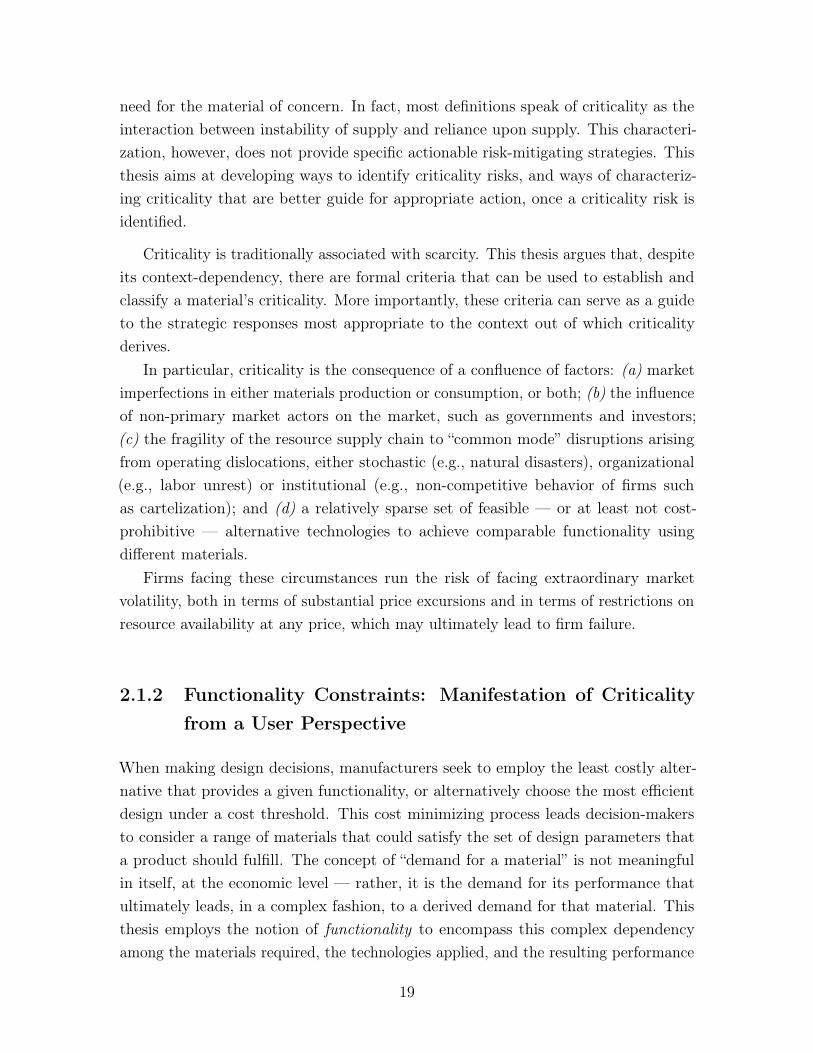
The topic of materials criticality has recently received attention largely because so-called “critical” materials, such as rare earth elements (REEs) and platinum groupmetals (PGMs), are of increasing importance for many different sectors of the economy:automotive, environmental, energy-related, high-technology etc. For instance, REEsare used in permanent magnets to make wind turbines, and PGMs are essential incatalytic converters needed to reduce car emissions. Recent studies have established alist of critical elements that is shown on Figure 2-1.

17

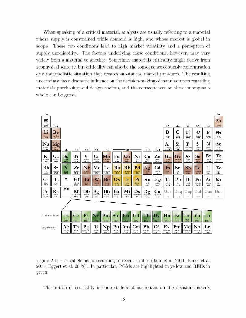
When speaking of a critical material, analysts are usually referring to a materialwhose supply is constrained while demand is high, and whose market is global inscope. These two conditions lead to high market volatility and a perception ofsupply unreliability. The factors underlying these conditions, however, may varywidely from a material to another. Sometimes materials criticality might derive fromgeophysical scarcity, but criticality can also be the consequence of supply concentrationor a monopolistic situation that creates substantial market pressures. The resultinguncertainty has a dramatic influence on the decision-making of manufacturers regardingmaterials purchasing and design choices, and the consequences on the economy as awhole can be great.

Figure 2-1: Critical elements according to recent studies (Jaffe et al. 2011; Bauer et al.2011; Eggert et al. 2008) . In particular, PGMs are highlighted in yellow and REEs ingreen.

The notion of criticality is context-dependent, reliant on the decision-maker’s

18

need for the material of concern. In fact, most definitions speak of criticality as theinteraction between instability of supply and reliance upon supply. This characteri-zation, however, does not provide specific actionable risk-mitigating strategies. Thisthesis aims at developing ways to identify criticality risks, and ways of characteriz-ing criticality that are better guide for appropriate action, once a criticality risk isidentified.

Criticality is traditionally associated with scarcity. This thesis argues that, despiteits context-dependency, there are formal criteria that can be used to establish andclassify a material’s criticality. More importantly, these criteria can serve as a guideto the strategic responses most appropriate to the context out of which criticalityderives.

In particular, criticality is the consequence of a confluence of factors: (a) marketimperfections in either materials production or consumption, or both; (b) the influenceof non-primary market actors on the market, such as governments and investors;(c) the fragility of the resource supply chain to “common mode” disruptions arisingfrom operating dislocations, either stochastic (e.g., natural disasters), organizational(e.g., labor unrest) or institutional (e.g., non-competitive behavior of firms suchas cartelization); and (d) a relatively sparse set of feasible — or at least not cost-prohibitive — alternative technologies to achieve comparable functionality usingdifferent materials.

Firms facing these circumstances run the risk of facing extraordinary marketvolatility, both in terms of substantial price excursions and in terms of restrictions onresource availability at any price, which may ultimately lead to firm failure.

2.1.2 Functionality Constraints: Manifestation of Criticalityfrom a User Perspective

When making design decisions, manufacturers seek to employ the least costly alter-native that provides a given functionality, or alternatively choose the most efficientdesign under a cost threshold. This cost minimizing process leads decision-makersto consider a range of materials that could satisfy the set of design parameters thata product should fulfill. The concept of “demand for a material” is not meaningfulin itself, at the economic level — rather, it is the demand for its performance thatultimately leads, in a complex fashion, to a derived demand for that material. Thisthesis employs the notion of functionality to encompass this complex dependencyamong the materials required, the technologies applied, and the resulting performance

19

of a manufactured good.

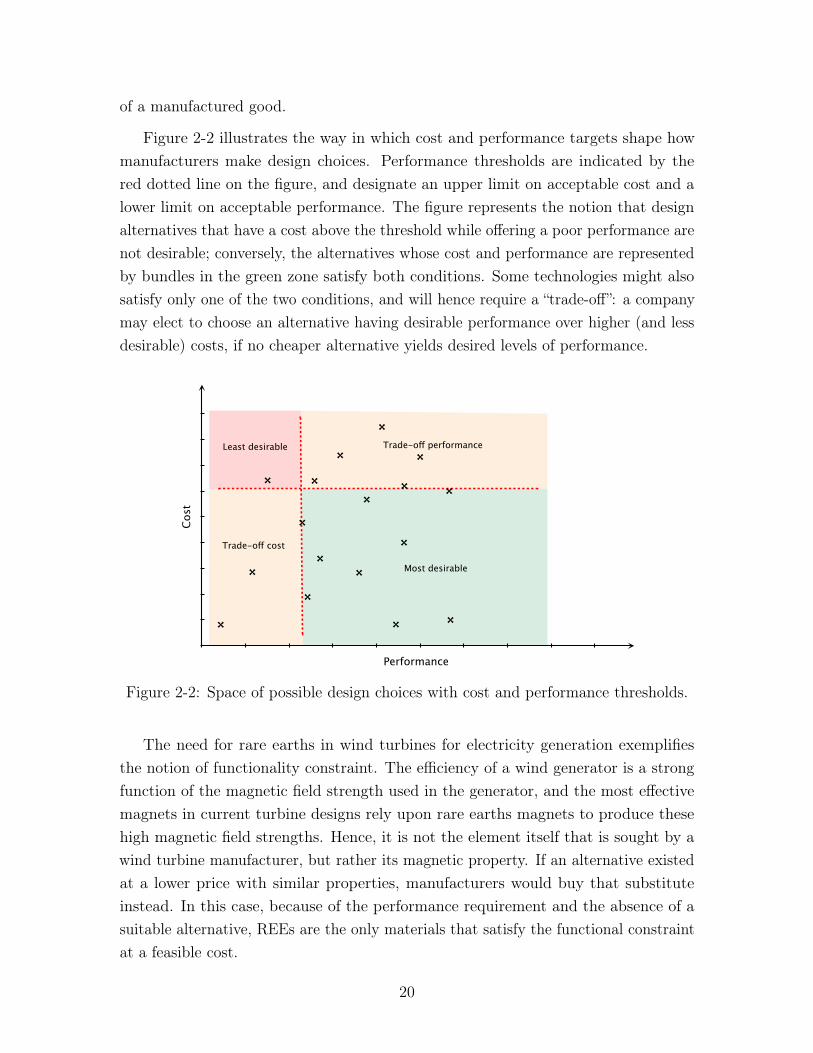
Figure 2-2 illustrates the way in which cost and performance targets shape howmanufacturers make design choices. Performance thresholds are indicated by thered dotted line on the figure, and designate an upper limit on acceptable cost and alower limit on acceptable performance. The figure represents the notion that designalternatives that have a cost above the threshold while offering a poor performance arenot desirable; conversely, the alternatives whose cost and performance are representedby bundles in the green zone satisfy both conditions. Some technologies might alsosatisfy only one of the two conditions, and will hence require a “trade-off”: a companymay elect to choose an alternative having desirable performance over higher (and lessdesirable) costs, if no cheaper alternative yields desired levels of performance.

Performance

Cos

t

Most desirable

Least desirable Trade-off performance

Trade-off cost

Figure 2-2: Space of possible design choices with cost and performance thresholds.

The need for rare earths in wind turbines for electricity generation exemplifiesthe notion of functionality constraint. The efficiency of a wind generator is a strongfunction of the magnetic field strength used in the generator, and the most effectivemagnets in current turbine designs rely upon rare earths magnets to produce thesehigh magnetic field strengths. Hence, it is not the element itself that is sought by awind turbine manufacturer, but rather its magnetic property. If an alternative existedat a lower price with similar properties, manufacturers would buy that substituteinstead. In this case, because of the performance requirement and the absence of asuitable alternative, REEs are the only materials that satisfy the functional constraintat a feasible cost.

20

Substitutes can be represented on the cost-performance matrix presented onFigure 2-2. Selecting a material over another becomes a matter of choosing which(performance–cost) bundle — represented as a black cross on the graph — is mostadvantageous, in the sense that it affords the producer the highest profitability as wellas provides the market a good that is attractive enough in terms of performance andsocial cost. In the case of critical materials however, the set of alternatives can be morelimited and constrained in specific ways that lead to criticality. In a case where thesupply for a specific material is unreliable for instance, its price may be subject to highvolatility, hence making the optimization process more challenging. More importantly,the set of alternatives may not be as abundant as it is for a non-critical material; inparticular, the functionality constraints might be predominant — in the case of REEsfor permanent magnets for instance — and hence no other known material could fulfillthe performance requirements.

Manufacturers need to account for criticality when making design and purchasingdecisions, because supply risks and price volatility greatly influence the market’sperception of availability. Failure to consider criticality might lead to situations, asin the case of palladium presented in Section 2.2, where historic price levels do notincorporate the notion that the supply for that material is constrained — for instancethe market is highly concentrated — and that this may lead to disruptive events suchas supply shortages or price excursions.

2.1.3 The Structure–Conduct–Performance Paradigm Appliedto Critical Materials Markets

As stressed in previous sections, critical elements can be of high importance to theeconomy as whole. In addition to market actors — in particular material producersand manufacturers — other stakeholders may also have a large interest in the stabilityof the market. As a result, not only do materials markets influence a large numberof stakeholders, but there can also be external influences on the market, exerted byactors outside the market, including governments.

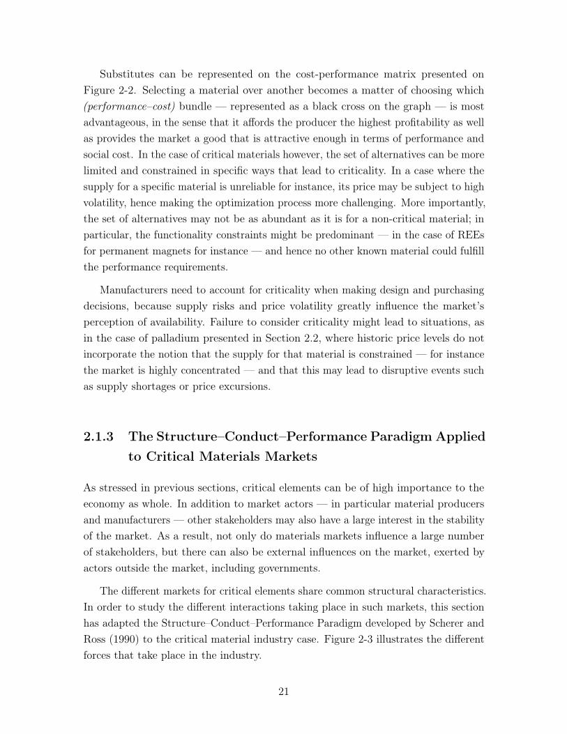
The different markets for critical elements share common structural characteristics.In order to study the different interactions taking place in such markets, this sectionhas adapted the Structure–Conduct–Performance Paradigm developed by Scherer andRoss (1990) to the critical material industry case. Figure 2-3 illustrates the differentforces that take place in the industry.

21

Market Structure

Market Conduct

Market Performance

Government Policy

Figure 2-3: The major components framing of the political economy of a materialsmarket, resulting from the Structure–Performance–Conduct paradigm. In particular,the arrows depict the ways in which the presented sectors influence one another.

The four main components of this framework are the market structure, conductand performance, as well as government policy1. The arrows on Figure 2-3 representthe influences exerted by the different blocks on each other, which will be described inthis section.

The broad definitions of each of the four components are summarized below:

Market Structure encompasses the architecture of the market: the number (andconcentration) of sellers and buyers, the barriers to entry (often very high in thecase of critical minerals since the mining industry is highly capital-intensive),and the cost structures of the different suppliers and consumers — i.e. theindividual supply and demand curves.

Market Conduct can be described, in the case of the mining industry, with firmpricing behavior, the potential for lobbying within the industry, as well as otherstructural components influencing the ways in which the market can behave —the notion of competitive advantage of different countries, for instance.

Market Performance can be described with the total materials production and theobservation of whether the market operates at the point of allocative efficiency(i.e. where marginal cost is equal to marginal benefit). Price volatility, sup-ply reliability and supply constancy are good indicators to assess the overallperformance of the market.

1One could also include the basic conditions of the market — namely the description of supplyand demand general characteristics, such as the physical constraints surrounding the material or theprice elasticity of demand. The scope of this study however is limited to the four main componentsof the paradigm.

22

Government Policy in the case of materials markets can take the form of taxes andsubsidies, international trade regulations, mining and environmental regulations,controls on the price of the commodities, or regulations against antitrust as wellas mandatory disclosure of information.

Because critical elements are important to a wide array of actors, the interactionsamong these four components will be large in number and diverse in their influence.Mapping them affords certain insights into the behavior of these markets.

Market Structure::Market Conduct The supply market for mineable materialsis generally highly concentrated — REEs are perhaps the most striking example,since 97% of the global supply is mined in China. Moreover, barriers to entryare very high in the mining industry, largely because of high investment costsand physical constraints. Monopoly or oligopoly may hence arise and lead tonon-competitive market behaviors. The monopolistic situation of China forREEs mining has given the country very strong bargaining powers, and therecent REE “crises” — in particular the setting of quotas and disruptions in thesupply (Bradsher 2010) — have arisen because of this inherent inefficiency inthe market structure. On the other hand, a concentrated demand side can leadto monopsony or oligopsony situations where a narrow sector dominates marketdemand. This can potentially increase the risk of lobbying by the main demandsector. Finally, extraction, refining and parts of the manufacturing phase can bevertically integrated for certain materials — it has recently become the case forthe permanent magnet industry using REEs for instance. The bargaining powerof one market actor may hence significantly increase and shift his behavior awayfrom what would be expected in a competitive market.

Conversely, the conduct on the market may also have an impact on the structure:demand sectors might drop out, or suppliers leave the market because of anaggressive pricing strategy that can be adopted by others. Again, the caseof REEs is striking: the monopoly situation observed until today mainly rosebecause other actors were driven out of business around 1985 when Chinaincreased its supply very significantly and drove prices down (Hurst 2010).

Government Policy::Market Structure Public policies may have a direct impacton the market structure, and this by different means. On the one hand, a materialcan be strategic to a government because of potential security implications; as aresult, the government itself may become a consumer and directly change the

23

structure of demand. On the other hand, policies can alter the very structure ofthe supply. First, governments can put in place antitrust regulations; in the caseof critical materials however, this lever can be limited in that the sometimeshighly concentrated situations on the market are due to either physical limitationsor the high financial barriers to entry. Governments may also have an incentiveto provide financial benefits to potential new entrants — via the use of subsidiesor specific taxation regimes for instance — and hence encourage the developmentof new mines that can alleviate the concentration of supply. Finally, governmentsmight be able to sanction reproved supply practices by regulating the sourcesof supply. The Dodd-Frank Act indeed requires all American manufacturers toreport any use of one of the 3TG materials (tantalum, tin, tungsten and gold)emanating from the Democratic Republic of Congo in its “Conflict Minerals”Rule (Dodd-Frank Act (2010)).

Government Policy::Market Conduct Different types of policy tools can be usedby governments to regulate critical materials markets and change their actors’behavior. One type of actions is the implementation of price controls; govern-ments may choose to either set a floor or a ceiling on the commodity price ifthey have sufficient authority, or to subsidize partly for the cost if the materialis deemed of high importance for national economy. Mining regulations mayalso be put in place so as to limit unreasonably high extraction rates that have anegative impact on (a) the environment, (b) the labor force and (c) other actorson the market that cannot operate at such high extraction rates. Public policiescan also tackle the question of asymmetric information on the market, which isa source of imperfections, and reduce this asymmetry by mandating informationdisclosures by suppliers — either directly or inferred through data collected fromthe firms comprising the overall industrial sector. Finally, regulations can beinfluenced by market actors who may benefit from a regulated environment, sincethey are usually better organized and have a greater influence on the politicalaspects of the economy. This can however weaken the efficiency of the markets,because of possible regulatory capture by private actors (Stigler 1971).

Market Conduct::Market Performance According to economic theory, the keyconditions of a perfectly competitive market are that information is perfect, thatactors behave rationally and homogeneously, and that there are no frictionsor transaction costs. Under these conditions, the market-clearing price shouldreflect the intrinsic economic value of the resource. As pointed out earlier, somemarket behaviors in the case of critical materials may lead to inefficiencies and

24

violate the assumptions of a perfectly competitive marketplace. The inefficienciesthat then arise — whether from the nature of the market, from the marketconditions specific to the material, or from external events such as conflicts — canhave an impact on the overall performance of the market. Events such as supplydisruptions, price volatility, or negative externalities, are direct consequences ofthose imperfections and can have dramatic impacts on the economy.

The market for critical materials presents systemic characteristics and inefficienciesthat make the supply chain for the resource vulnerable to risks such as supply disruptionor high price volatility.

2.2 Illustration of the Concept of Criticality: the Ex-ample of Palladium

One of the most acute market imperfections for critical materials is the incompletenessof information. The supply for critical materials is concentrated in a limited numberof countries, while their market is very often global. Concentration gives supplyingcountries additional bargaining power at the international level and increases thedependence of importing nations on the information coming from a limited numberof major actors. Manufacturers have to plan their expected consumption for theupcoming year and order an adequate quantity from the exporting countries. Contracts(short- or long-term, depending on the producing countries) can be established, butsupply disruptions are possible. Furthermore, the global demand for one materialin a year can be challenging to estimate for market strategists, since it depends ontechnological changes, new regulations — such as CAFE standards that raise theneed for PGMs in catalytic converters — investors, price etc. The incompleteness ofinformation — and in particular the asymmetry of information concerning the supplythe limited understanding of mine operations and deposits by manufacturers — leadsto inefficiencies on the market.

Palladium, one of the six PGMs, is an interesting example of critical material. Inparticular, the “Palladium Crisis” of 1998 provides a good illustration of a specificaspect of criticality, namely that of asymmetry of information perpetrated by an actorof the supply duopoly for the material, combined with an unprecedented increase indemand.

The following sections use the palladium case to illustrate how ‘criticality’ should

25

be studied specifically in order to identify the different causes and interactions thatled to a critical market.

2.2.1 The “Palladium Crisis”: Origin and Implications

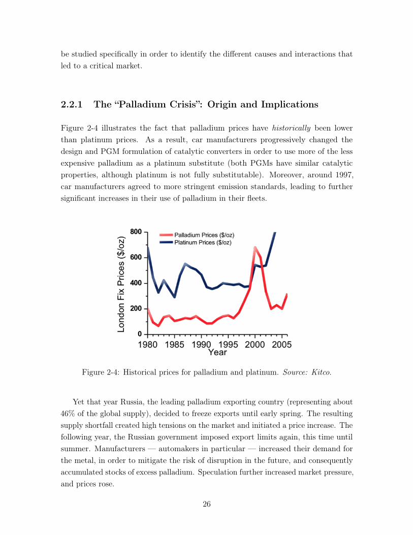
Figure 2-4 illustrates the fact that palladium prices have historically been lowerthan platinum prices. As a result, car manufacturers progressively changed thedesign and PGM formulation of catalytic converters in order to use more of the lessexpensive palladium as a platinum substitute (both PGMs have similar catalyticproperties, although platinum is not fully substitutable). Moreover, around 1997,car manufacturers agreed to more stringent emission standards, leading to furthersignificant increases in their use of palladium in their fleets.

Figure 2-4: Historical prices for palladium and platinum. Source: Kitco.

Yet that year Russia, the leading palladium exporting country (representing about46% of the global supply), decided to freeze exports until early spring. The resultingsupply shortfall created high tensions on the market and initiated a price increase. Thefollowing year, the Russian government imposed export limits again, this time untilsummer. Manufacturers — automakers in particular — increased their demand forthe metal, in order to mitigate the risk of disruption in the future, and consequentlyaccumulated stocks of excess palladium. Speculation further increased market pressure,and prices rose.

26

When the anticipated supply disruption did not take place and demand shiftedaway from palladium — some industries managed to reduce their demand by designchanges that proved very costly — the price of palladium dropped abruptly andmanufacturers with large inventories of unused palladium incurred major losses. Togive a sense of the magnitude of these losses, one major US car manufacturer lostover one billion dollars during that crisis — and on average, less than an ounce ofpalladium is used in a car.

This crisis illustrates how the combination of different events made palladiumparticularly critical:

On the one hand, expectations of actors were not met, in that the past provedinsufficient to inform the future behavior of the market. Indeed, the demand forpalladium increased significantly around that time, mainly due to the early and rapidadoption of stringent new emission regulations by car manufacturers that expectedpalladium supply to be abundant enough to meet their needs — as had always beenthe case by the past. When the Russian government cut the supply, the demand couldnot be met, the other sources of supply (mainly South African and North Americanless significantly) proved insufficient to sustain the surge in demand, leading prices torise.

On the other hand, there was a significant asymmetry of information concerningthe Russian supply.

The first manifestation of it came from the quotas set by the government. Itshould be noted that all of the Russian primary PGMs supply comes from the Norilsknickel mine (of which PGMs are byproducts). Furthermore, all the exports have tobe processed through Almazjuvelirexport, a federal state-owned unitary enterprise,exporting precious metals on a commission basis. The supply cuts that occurred in1997 and 1998 had been publicly justified as resulting from paperwork processingissues within the governmental instances. The government hence played an importantrole in the supply disruptions that occurred at that time and did not provide sufficientand accurate information about the quotas that had been set — in a timely fashionfor decision-makers to make informed purchasing decisions.

The second very important source of incomplete information in the case of theRussian palladium supply is the existence of a strategic stock in Russia. In the 1970sand 1980s, during the Cold War, a lot of palladium had been extracted in the nickelmine. Yet at the time, the demand for palladium was very slim and trading thatprecious metal only seemed secondary in the eyes of the soviet government. As a result,important quantities of that material got piled up in national reserves and remainedthere under state secrecy until the growing need for palladium provided an incentive to

27

the Russian government to start trading that stock. In the years preceding the crisis,palladium had been flowing out of that stock as well in order to meet growing exportrequirements. But the quantity remaining in that stock had always been treated asa very important state secret, and manufacturers importing Russian palladium didnot know exactly how much metal was left . Hence, purchasing teams were planningtheir import quantities based on the supply from previous years and accounting forthe strategic stock to fulfill their needs. This lack of information and transparencyfrom Russia only further increased the negative effects of the crisis, and speculatorsused it in order to deepen the pressure on the market and palladium prices.

In this case, criticality arose because of the combination of different factors. First,the historical demand data was not sufficient to inform future consumption because ofradical changes in the automotive industry that led to a significantly higher reliance onpalladium. Second, uncertainty surrounded the Russian exports, since the governmentset export quotas and the magnitude of the stock remained (and still is today) unknown.This asymmetry of information became egregious because Russia was responsible fora large part of the global supply.

Uncertainty surrounding both supply and demand, led to very high price volatility,market instability — worsened by investors — and ultimately encouraged the devel-opment of North American mines (Stillwater in particular) so as to ease the marketconcentration.

2.2.2 Risk-Mitigating Policies that were Implemented at theTime

On the one hand, palladium consumers implemented different policies to mitigate therisks and the impacts on the market.

First, manufacturers decided to stockpile when Russia announced supply disrup-tions. This policy turned out to be very harmful because that stock was constitutedwhen the price was rising, but it quickly fell at its original level, hence significantlydevaluating the investment made by the manufacturers.

Then design choices were made so as to move away from palladium as quicklyas possible; some car manufacturers developed very expensive new design strategiesto be able to meet newly established stringent regulation standards without usingas much palladium. Similarly, electronics companies tried to reduce the amount ofpalladium used. Because the decisions were made very rapidly and changes had tobe implemented sometimes in less than a one-year period, these changes were very

28

expensive to implement.Achieving increased recovery and recycling of palladium might have been an efficient

policy, since a secondary source of supply tends to mitigate supply disruption risks.However, that could not be put into place at that time because the widespread use ofpalladium in car was a very recent development. Without a stock of obsolete productfrom which to extract material, there was no palladium to recycle.

The supply side also put different policies into place. In 1999, the Russiangovernment authorized long-term contracts (10 years) with automakers in order toease the market panic, and lifted the quotas on primary exports. Exports from thestock had to be individually reviewed, but that measure eased the market to a certainextent. Finally, investors decided to expand the Stillwater mine, while other sourcesof supply emerged (in Canada and Zimbabwe), reducing market concentration via a“natural” market structural change.

2.2.3 Proposed Policy Options to Lower the Impact of Infor-mation Asymmetry on the Market

The market for critical materials, and palladium in particular, typically owes itsconcentration to natural causes: not every material can be economically extractedeverywhere, and opening a mine represents a massive investment. As a result, first-movers and countries where a material is particularly abundant and easily mineablehave a definite strategic advantage. Russia is a major player in the market forpalladium, and hence greatly influences it. The Russian government has had a stronginfluence on the treatment of palladium exports, which has increased the asymmetryof information concerning quota setting as well as quantity of stock remaining. Indeed,all exports have to go through one state-owned company and every transaction hasto be approved by the government. Moreover, the paperwork and export approvalsrequired to unfreeze the Russian supply were a very good example of what Allison(1969) qualifies as organizational inefficiencies: the government had to follow the pre-established the “standard operating procedures” despite the exceptional circumstancescreated by an increase in demand, which limited the choices and hence the strategiesthat could be adopted. Other governments cannot intervene to directly reduce theinformation asymmetry however — especially because Russia was not in the WTOat the time (it entered in August 2012) hence limiting the bargaining power of theinternational community.

Different public policies can be considered in order to mitigate the risk created

29

by the asymmetry of information. The first one is aimed at reducing the informationasymmetry by gaining more control over supply information; this can be accomplishedby the opening of a new mine — if the reserves exist — in an importing country, sincepossessing a domestic source of an expensive commodity can prove very strategic. Thisis what happened in the United States with a significant expansion of the Stillwatermine under a federal mining law that provides subsidies for purchasing of public land.The main drawback of this policy is the very high upfront cost it requires — notnecessarily by the government, but by the investors building the mine. Hence it is notalways a feasible option. Another way to accomplish that same goal yet to a lesserextent could be through the investment in an existing mine that would not have to bedomestic, hence providing a greater control on the operations of the mine. It would bechallenging to implement since mining countries may not accept other governments’investments, but could potentially be accomplished by private companies.

Another type of policy would be the creation of a federal stock of the materialsdeemed strategic. Of course, with this policy come the drawbacks of the riskyinvestments and it can be seen as an overregulation of which the costs might exceedthe benefits, if the investment proves hazardous.

One could also envision the negotiation of governmental contracts for the regulationof imports/exports that could act as insurance policies for domestic manufacturersin need of a critical material. Yet such a policy would require an important amountof coordination amongst the nations, which could be problematic in cases similar tothe one we just studied where it seemed that coordination was lacking even withinthe Russian government to get the different approvals. Moreover, one could arguethat such an insurance policy would be risky for a government to take on, and shouldbe implemented only if the material impacts industries that have a strategic role inthe domestic economy. The strategic importance of PGMs and the impact it has onseveral industries — including high-technology industry — could lead governmentsto, in fact, take action. It could however increase the risk of a Stiglerian regulatorycapture (Stigler 1971) by industries that are in need of a specific material, since thoseinterest groups would benefit from regulations favoring their own industry throughsubsidized raw products, as compared to others that may not need the same materials.

Finally, asymmetry of information could be eased by structures in charge ofmonitoring extraction and demand evolutions. Certain organizations, such as JohnsonMatthey for PGMs or the United States Geological Survey (USGS), publish periodicalreports and data about the state of the market of various materials. Yet these reportsusually provide a short-term outlook on both production and demand, which doesnot provide sufficient information for decision-makers to make purchasing decisions in

30

a timely fashion. It would hence be beneficial to have an international third-partyorganization that publishes comprehensive reports with longer-term considerations tohelp industries make decisions about materials.

Asymmetry of information in the context of extraction of critical materials isan important source of market failure; mitigating that risk can prove challengingwhen the supply is controlled by the government of main suppliers. However somepublic policies can be put in place within importing nations so as to limit the impactson manufacturers and, were the mines not directly controlled by the government,policies within mining countries could be implemented in order to maintain minimumcontractual exports, which could be supported by the WTO for instance. In any case,appropriate risk-assessment should be developed.

The example of palladium, and more specifically of the 1998 “Palladium Crisis”, isan illustration of a specific case of criticality. Indeed, palladium became critical aroundthat time because of an increased demand — fostered by the automotive industry andtightened emission regulations — as well as a complex and uncertain supply streamemanating mainly from Russia. This example hence illustrates a specific aspect ofwhat we previously defined as materials criticality.

2.3 A Review of Existing Approaches to the Ques-tion of Criticality

The notion of criticality has been formally addressed only recently (Erdman andGraedel 2011) — resource scarcity had been widely studied in the past, but the notionthat factors other than depletion can affect the reliability of materials’ supply hasonly emerged recently, with the manifestation of large economic crises such as the onepresented in Section 2.2.

This section will present an overview of existing criticality-assessment methods,and illustrate where this work adds to the existing body of methods.

2.3.1 Past Work on Material Criticality

General Considerations

The notion of criticality is difficult to formalize, since, as mentioned earlier, it is verysubjective; however existing approaches agree on a fundamental issue, namely the fact

31

that criticality is a manifestation of a supply risk and of a vulnerability to this risk(Graedel et al. 2011; Bauer et al. 2011; Jaffe et al. 2011).

The question of supply risk is now widely recognized as not limited only to scarcity(as mentioned in the report Critical Raw Materials for the EU 2010). Instead, otherconsiderations (such as geopolitical risks or sustainability concerns, as presented byGraedel et al. 2011) are often mentioned when assessing the question of supply riskscomprehensively. The sources of concern that are highlighted in recent works can bevery diverse: including relative physical availability (often evaluated by the USGS2),feasibility of extraction, regulations and societal characteristics of producing countries(Graedel et al. 2011, mentions the Human Development Index for instance), andgeopolitical considerations that can be measured using metrics such as the HHI3. Mostapproaches tackle the issue of supply risk assessment through the construction anduse of metrics, presented in the next section.

Another important notion for criticality is that of the “functionality constraints”that we mentioned in Section 2.1, or vulnerability to risk. This notion is oftenaddressed by defining the scope of the study, and in particular by specifying who thestakeholder is and what his specific current or projected demand for the material is —the scope is determinant in deciding which materials are critical and which are not(Erdman and Graedel 2011). The question of materials substitutability is also veryimportant for manufacturers, since it directly feeds into the design decision-makingprocess, and is hence helps to establish the demand-related risks of a material. Anotherimportant aspect of demand risks is the structure of the demand — more specifically,the concentration of demand sectors, and the resulting market power of suppliers overa specific decision-maker.

Finally, the notion of time dependency of criticality assessment is cited as animportant consideration (in the report Bauer et al. 2011, for instance). A criticalassessment has indeed a short ‘lifetime’, since the context in which it is establishedis subject to evolving influences. Therefore, criticality assessment must be regularlyupdated to reflect changing market contexts.

2United States Geological Survey, a scientific American agency that study among others naturalresources

3The Herfindahl–Hirschman Index that measures the relative competition of firms in a market bycomparing individual sizes to the industry as a whole, and defined in the following section.

32

Metrics-Based Approaches

A large portion of the literature on criticality relies on the use of metrics, to assess thecriticality risks presented by a specific material. In these analyses, the decision-makercollects relevant data and computes different numerical indicators that indicate towhat extent a particular aspect of the market presents a risk.

One of the particularities of such approaches is the ease of computation, since thedata necessary to calculate such metrics can be found in publicly available sources,such as the annual reports of mining operations or surveys such as the United StatesGeological Survey (USGS). Another type of resource can be annual overviews of aspecific market by private consulting firms — for instance Johnson Matthey for PGMs.

Moreover, a decision-maker can easily refine such a risk assessment to his require-ments by choosing the metrics that are most relevant to his activity and need, as wellas setting the appropriate thresholds that lead to declaring that the material is criticalfor his firm, or not. This degree of customization makes a metrics-based criticalityassessment particularly flexible, as well as quick.

Examples of metrics that are often cited and used are listed below:

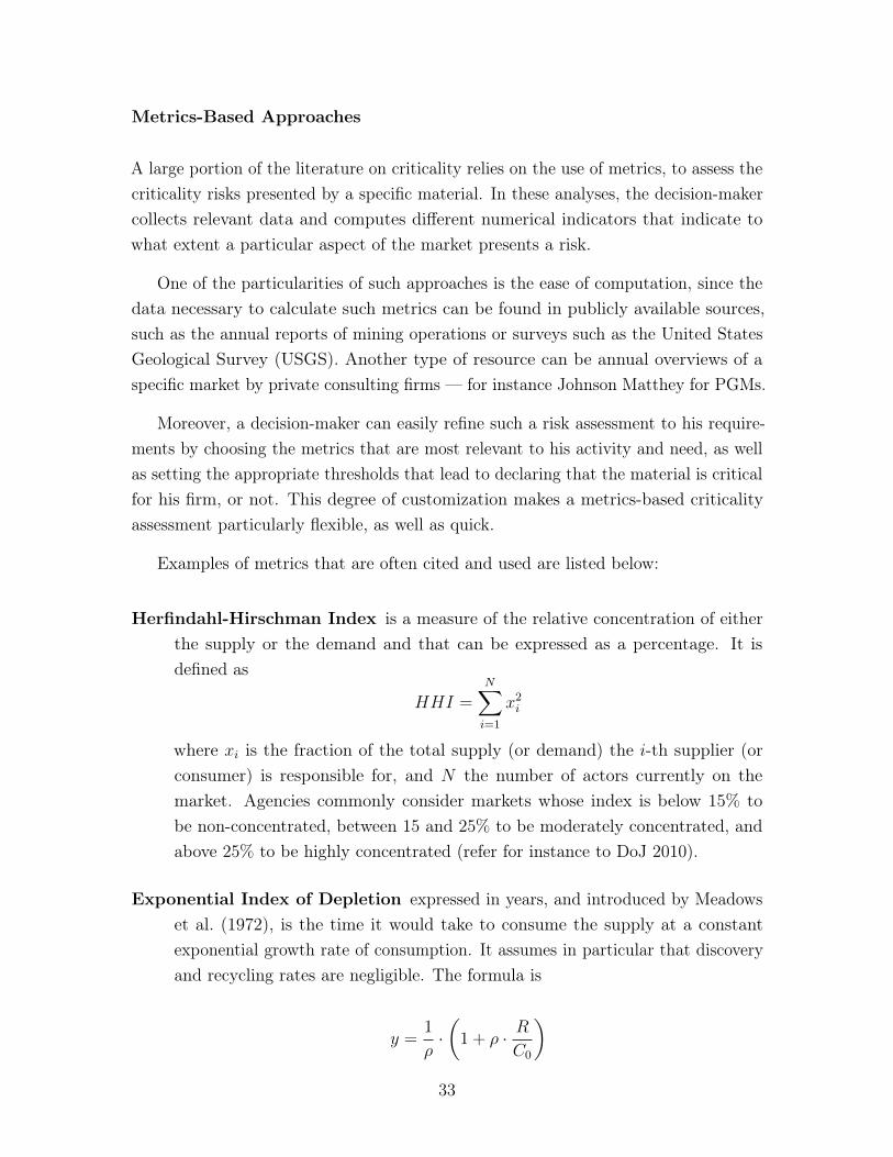
Herfindahl-Hirschman Index is a measure of the relative concentration of eitherthe supply or the demand and that can be expressed as a percentage. It isdefined as

HHI =

NX

i=1

x2i

where xi

is the fraction of the total supply (or demand) the i-th supplier (orconsumer) is responsible for, and N the number of actors currently on themarket. Agencies commonly consider markets whose index is below 15% tobe non-concentrated, between 15 and 25% to be moderately concentrated, andabove 25% to be highly concentrated (refer for instance to DoJ 2010).

Exponential Index of Depletion expressed in years, and introduced by Meadowset al. (1972), is the time it would take to consume the supply at a constantexponential growth rate of consumption. It assumes in particular that discoveryand recycling rates are negligible. The formula is

y =

1

⇢·✓1 + ⇢ · R

C0

◆

33

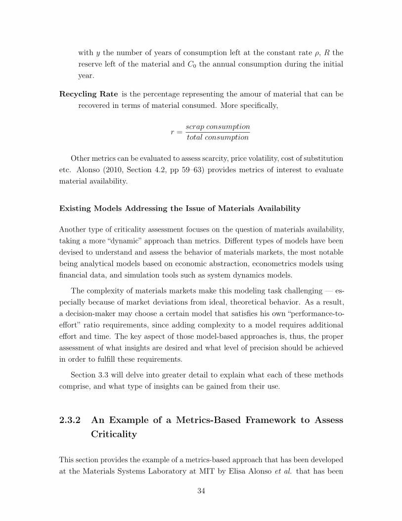
with y the number of years of consumption left at the constant rate ⇢, R thereserve left of the material and C0 the annual consumption during the initialyear.

Recycling Rate is the percentage representing the amour of material that can berecovered in terms of material consumed. More specifically,

r =scrap consumption

total consumption

Other metrics can be evaluated to assess scarcity, price volatility, cost of substitutionetc. Alonso (2010, Section 4.2, pp 59–63) provides metrics of interest to evaluatematerial availability.

Existing Models Addressing the Issue of Materials Availability

Another type of criticality assessment focuses on the question of materials availability,taking a more “dynamic” approach than metrics. Different types of models have beendevised to understand and assess the behavior of materials markets, the most notablebeing analytical models based on economic abstraction, econometrics models usingfinancial data, and simulation tools such as system dynamics models.

The complexity of materials markets make this modeling task challenging — es-pecially because of market deviations from ideal, theoretical behavior. As a result,a decision-maker may choose a certain model that satisfies his own “performance-to-effort” ratio requirements, since adding complexity to a model requires additionaleffort and time. The key aspect of those model-based approaches is, thus, the properassessment of what insights are desired and what level of precision should be achievedin order to fulfill these requirements.

Section 3.3 will delve into greater detail to explain what each of these methodscomprise, and what type of insights can be gained from their use.

2.3.2 An Example of a Metrics-Based Framework to AssessCriticality

This section provides the example of a metrics-based approach that has been developedat the Materials Systems Laboratory at MIT by Elisa Alonso et al. that has been

34

applied during this research work in order to quickly evaluate the criticality of differentmaterials for a manufacturer.

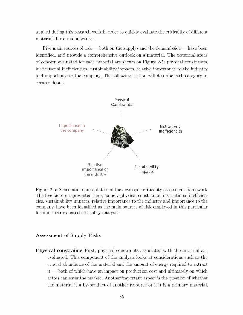
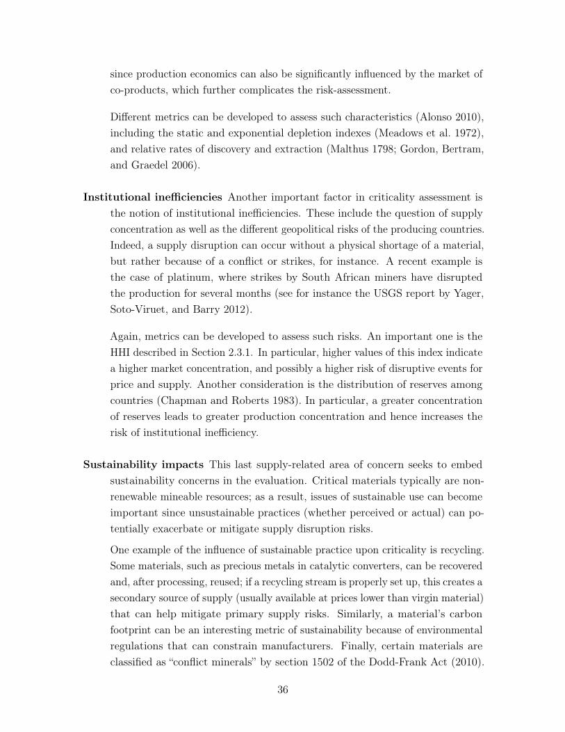
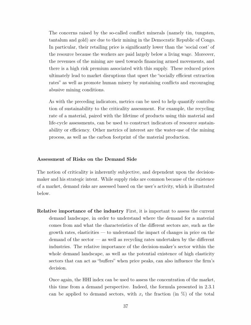
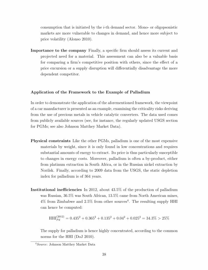
Five main sources of risk — both on the supply- and the demand-side — have beenidentified, and provide a comprehensive outlook on a material. The potential areasof concern evaluated for each material are shown on Figure 2-5: physical constraints,institutional inefficiencies, sustainability impacts, relative importance to the industryand importance to the company. The following section will describe each category ingreater detail.

Figure 2-5: Schematic representation of the developed criticality-assessment framework.The five factors represented here, namely physical constraints, institutional inefficien-cies, sustainability impacts, relative importance to the industry and importance to thecompany, have been identified as the main sources of risk employed in this particularform of metrics-based criticality analysis.

Assessment of Supply Risks

Physical constraints First, physical constraints associated with the material areevaluated. This component of the analysis looks at considerations such as thecrustal abundance of the material and the amount of energy required to extractit — both of which have an impact on production cost and ultimately on whichactors can enter the market. Another important aspect is the question of whetherthe material is a by-product of another resource or if it is a primary material,

35

since production economics can also be significantly influenced by the market ofco-products, which further complicates the risk-assessment.

Different metrics can be developed to assess such characteristics (Alonso 2010),including the static and exponential depletion indexes (Meadows et al. 1972),and relative rates of discovery and extraction (Malthus 1798; Gordon, Bertram,and Graedel 2006).

Institutional inefficiencies Another important factor in criticality assessment isthe notion of institutional inefficiencies. These include the question of supplyconcentration as well as the different geopolitical risks of the producing countries.Indeed, a supply disruption can occur without a physical shortage of a material,but rather because of a conflict or strikes, for instance. A recent example isthe case of platinum, where strikes by South African miners have disruptedthe production for several months (see for instance the USGS report by Yager,Soto-Viruet, and Barry 2012).

Again, metrics can be developed to assess such risks. An important one is theHHI described in Section 2.3.1. In particular, higher values of this index indicatea higher market concentration, and possibly a higher risk of disruptive events forprice and supply. Another consideration is the distribution of reserves amongcountries (Chapman and Roberts 1983). In particular, a greater concentrationof reserves leads to greater production concentration and hence increases therisk of institutional inefficiency.

Sustainability impacts This last supply-related area of concern seeks to embedsustainability concerns in the evaluation. Critical materials typically are non-renewable mineable resources; as a result, issues of sustainable use can becomeimportant since unsustainable practices (whether perceived or actual) can po-tentially exacerbate or mitigate supply disruption risks.

One example of the influence of sustainable practice upon criticality is recycling.Some materials, such as precious metals in catalytic converters, can be recoveredand, after processing, reused; if a recycling stream is properly set up, this creates asecondary source of supply (usually available at prices lower than virgin material)that can help mitigate primary supply risks. Similarly, a material’s carbonfootprint can be an interesting metric of sustainability because of environmentalregulations that can constrain manufacturers. Finally, certain materials areclassified as “conflict minerals” by section 1502 of the Dodd-Frank Act (2010).

36

The concerns raised by the so-called conflict minerals (namely tin, tungsten,tantalum and gold) are due to their mining in the Democratic Republic of Congo.In particular, their retailing price is significantly lower than the ‘social cost’ ofthe resource because the workers are paid largely below a living wage. Moreover,the revenues of the mining are used towards financing armed movements, andthere is a high risk premium associated with this supply. These reduced pricesultimately lead to market disruptions that upset the “socially efficient extractionrates” as well as promote human misery by sustaining conflicts and encouragingabusive mining conditions.

As with the preceding indicators, metrics can be used to help quantify contribu-tion of sustainability to the criticality assessment. For example, the recyclingrate of a material, paired with the lifetime of products using this material andlife-cycle assessments, can be used to construct indicators of resource sustain-ability or efficiency. Other metrics of interest are the water-use of the miningprocess, as well as the carbon footprint of the material production.

Assessment of Risks on the Demand Side

The notion of criticality is inherently subjective, and dependent upon the decision-maker and his strategic intent. While supply risks are common because of the existenceof a market, demand risks are assessed based on the user’s activity, which is illustratedbelow.

Relative importance of the industry First, it is important to assess the currentdemand landscape, in order to understand where the demand for a materialcomes from and what the characteristics of the different sectors are, such as thegrowth rates, elasticities — to understand the impact of changes in price on thedemand of the sector — as well as recycling rates undertaken by the differentindustries. The relative importance of the decision-maker’s sector within thewhole demand landscape, as well as the potential existence of high elasticitysectors that can act as “buffers” when price peaks, can also influence the firm’sdecision.

Once again, the HHI index can be used to assess the concentration of the market,this time from a demand perspective. Indeed, the formula presented in 2.3.1can be applied to demand sectors, with x

i

the fraction (in %) of the total

37

consumption that is initiated by the i-th demand sector. Mono- or oligopsonisticmarkets are more vulnerable to changes in demand, and hence more subject toprice volatility (Alonso 2010).

Importance to the company Finally, a specific firm should assess its current andprojected need for a material. This assessment can also be a valuable basisfor comparing a firm’s competitive position with others, since the effect of aprice excursion or a supply disruption will differentially disadvantage the moredependent competitor.

Application of the Framework to the Example of Palladium

In order to demonstrate the application of the aforementioned framework, the viewpointof a car manufacturer is presented as an example, examining the criticality risks derivingfrom the use of precious metals in vehicle catalytic converters. The data used comesfrom publicly available sources (see, for instance, the regularly updated USGS sectionfor PGMs; see also Johnson Matthey Market Data).

Physical constraints Like the other PGMs, palladium is one of the most expensivematerials by weight, since it is only found in low concentrations and requiressubstantial amounts of energy to extract. Its price is thus particularly susceptibleto changes in energy costs. Moreover, palladium is often a by-product, eitherfrom platinum extraction in South Africa, or in the Russian nickel extraction byNorilsk. Finally, according to 2009 data from the USGS, the static depletionindex for palladium is of 364 years.

Institutional inefficiencies In 2012, about 43.5% of the production of palladiumwas Russian, 36.5% was South African, 13.5% came from North American mines,4% from Zimbabwe and 2.5% from other sources4. The resulting supply HHIcan hence be computed:

HHI(2012)Pd

= 0.4352 + 0.3652 + 0.1352 + 0.042 + 0.0252 = 34.3% > 25%

The supply for palladium is hence highly concentrated, according to the commonnorms for the HHI (DoJ 2010).

4Source: Johnson Matthey Market Data

38

As mentioned in Section 2.2, this high concentration as well as the Russiangeopolitical landscape have led to supply disruption and high price volatility inthe past. Moreover, recent strikes in South Africa have added pressure on themarket5.

Sustainability impacts Russia mainly relies on nuclear, hydropower and naturalgas to produce its electricity; however, given the high energy needed to extractpalladium, as well as South Africa’s reliance on coal-powered electricity gen-eration, the palladium’s carbon footprint is very large. Recycling mitigatesthis footprint somewhat, especially because the recycling of palladium is fairlyefficient and well-established. Moreover, its use in catalytic converters also helpsreducing NO

x

and CO2

. Finally, palladium does not pose significant conflictmineral risks.

Relative importance of the industry Recent growth in car sales in Europe andSouth America has driven up the palladium demand for 2011 (a 6% increase).Moreover, the increasing Asian production of gasoline vehicles is a major influenceon palladium’s prices. Although the demand for palladium in the chemical andelectrical industries has risen, the automotive industry still constitutes themain demand driver for this metal. Jewelry demand is forecast to decrease aspalladium prices rise, acting as a “buffer” sector to a certain extent, and hencelowering the impact of price excursions or other supply disruptions on otherdemand sectors.

This cursory criticality assessment, based on metrics and qualitative data, and tobe completed with the specific needs of a given manufacturer, illustrates the criticalityof palladium as a material used massively in the automotive industry as well as inother sectors.

While the resulting risk-profile for palladium is useful to quickly realize thatpalladium can, indeed, be critical if the firm’s demand for that resource is significant,the scope of this assessment is limited, since only static measures are considered. Inparticular, devising well-informed mitigation strategies can be challenging with onlymetrics-based considerations. Section 2.3.3 below addresses in greater details thegeneral limitation of metrics-based approaches, such as the one presented here.

5A report on the impact of the strikes on the PGM industry has been published by the USGS(Yager, Soto-Viruet, and Barry 2012). An interesting analysis focused on palladium has also beenpublished by Thomson Reuters GFMS (2013).

39

2.3.3 Addressing the Gaps in the Current Approaches to Crit-icality

Limitations of Static Approaches

The metrics-based approaches present the very significant advantage of being easilycomputable, easy to compare, as well as requiring a limited amount of data. However,they present several drawbacks that reduce their efficiency at comprehensively assessingmaterials’ criticality.

First, metrics are inherently static. Some metrics may include a dynamic aspectby considering several years and including discount rate considerations, such as thedynamic depletion index. Nevertheless, metrics can only be evaluated at one pointin time and hence cannot capture the existing complex interactions among supply,demand, and price. Section 4.2 will provide examples of situations when static metricsapproaches are limited, and when the use of a dynamic approach such as a model canhelp better inform a decision-maker about the market.

In addition, the use of metrics requires a decision-maker to decide (a) what metricsto use and (b) where to set the thresholds to establish that a material is critical.It is incumbent on the decision-maker to make such “judgment calls”, which canbe difficult to make consistently. Moreover, changes in market circumstances mayrequire the establishment of new thresholds, or the use of different metrics. As aresult, metrics-based approaches may need constant revision, not only to modify thecontext as for other criticality-assessment methods, but also to adjust the frameworkitself. Moreover, metrics may not be sufficient to comprehensively understand marketdynamics and resulting risks.

Limitations of Existing Modeling Approaches

Section 3.3 will provide a more detailed overview of the limitations of existing modelingapproaches, but the main issues are that most of the tools developed are either toodata- and resource-intensive — especially system dynamics tools — or use an economicabstraction that neither accounts for market imperfections, nor provide the short-termvision that may be required by manufacturers.

40

Proposed Method to Address These Concerns

Metrics are a quick and easily computable way of assessing materials criticality, byevaluating the extent to which a material presents a given risk. Yet such approach isinherently static and ignores market dynamics that can take place and exacerbate ormitigate risks that would be harmful to a manufacturer.

While modeling tools are inherently limited in that they cannot fully replicatereality and might be extremely resource-intensive, they can address many of thelimitations of metrics-based approaches. They can at a minimum be used to augmentand complement these analyses by affording further insights. The question arises ofthe trade-off between the amount of effort required to build the modeling tool and thequality of insight that can be extracted from its use. Depending on a decision-maker’sneeds and the scope of his criticality study, different models may be favored over others.Yet it is not always straightforward to assess the criticality of multiple materials, sinceit may require a large amount of effort.

Based on those considerations, this work proposes a two-tiered approach to theassessment of materials criticality and the development of risk-mitigating policies thatcan be implemented by a decision-maker.

- First, a risk-profile of the material can be easily developed by using a frameworksimilar to the one described in the section 2.3.2. This will enable the decision-maker to quickly assess, with the use of publicly available data, whether or nota material presents a potential risk to his activity.

- Then, if the risk is deemed significant, a market model has been designed to(a) use economics theory to understand market dynamics, (b) incorporate marketimperfections that will improve the realism of the model and (c) use only alimited amount of data and be sufficiently flexible, in order to be applicable todifferent materials. The tool has been built in particular to make it easy for itsuser to compare different scenarios.

The following chapter presents the modeling tool that has been developed toanswer the need for such a modeling tool, which addresses the different concerns ofmetrics-based approaches and adds to the existing modeling approaches.

41

42

Chapter 3

Methodology

This chapter introduces the modeling tool that has been developed in order to tackle thequestion of materials criticality while taking market dynamics into account. This tool,the Materials Mining Market Model for Manufacturers (or m:5) has been groundedin economic theory, but also incorporates the knowledge we have of mining marketsand, in particular, accounts for some types of market imperfections. Moreover, themodel has been built so that it requires only a limited amount of inputs, making itequally applicable to a wide range of materials markets. Finally, the model was builton a spreadsheet platform for accessibility.

In the following description of the modeling methodology, we will first present theeconomic reasoning used to build the model, as well as the different characteristicsspecific to the mining industry that have been implemented in order to capturecharacteristic market imperfections. Then the tool developed will be compared toother existing models that also describe materials market, and the practical as well astheoretical differences that can be observed will be discussed. Finally, this section willpresent the implementation of the model, as well as the assumptions used.

3.1 Model Design Philosophy

This section addresses the motivations that lead to the elaboration of the m:5 model,especially concerning the construction of the supply curves and the market-clearingmechanism.

43

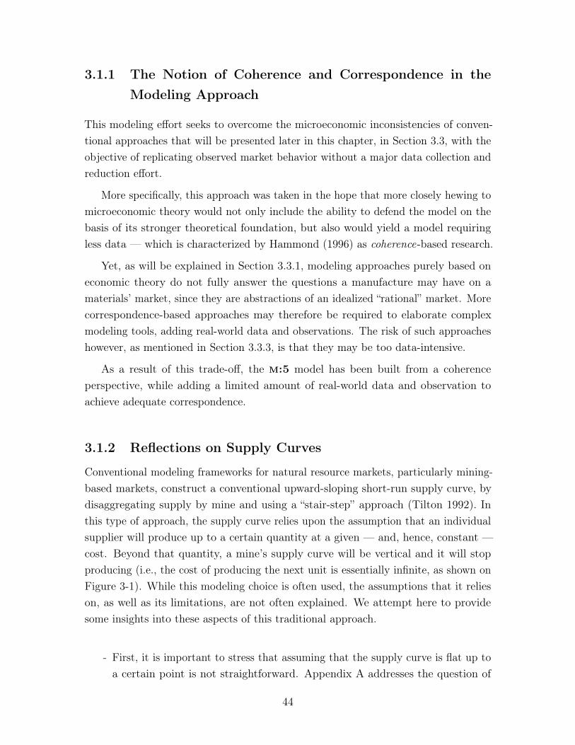
3.1.1 The Notion of Coherence and Correspondence in theModeling Approach

This modeling effort seeks to overcome the microeconomic inconsistencies of conven-tional approaches that will be presented later in this chapter, in Section 3.3, with theobjective of replicating observed market behavior without a major data collection andreduction effort.

More specifically, this approach was taken in the hope that more closely hewing tomicroeconomic theory would not only include the ability to defend the model on thebasis of its stronger theoretical foundation, but also would yield a model requiringless data — which is characterized by Hammond (1996) as coherence-based research.

Yet, as will be explained in Section 3.3.1, modeling approaches purely based oneconomic theory do not fully answer the questions a manufacture may have on amaterials’ market, since they are abstractions of an idealized “rational” market. Morecorrespondence-based approaches may therefore be required to elaborate complexmodeling tools, adding real-world data and observations. The risk of such approacheshowever, as mentioned in Section 3.3.3, is that they may be too data-intensive.

As a result of this trade-off, the m:5 model has been built from a coherenceperspective, while adding a limited amount of real-world data and observation toachieve adequate correspondence.

3.1.2 Reflections on Supply Curves

Conventional modeling frameworks for natural resource markets, particularly mining-based markets, construct a conventional upward-sloping short-run supply curve, bydisaggregating supply by mine and using a “stair-step” approach (Tilton 1992). Inthis type of approach, the supply curve relies upon the assumption that an individualsupplier will produce up to a certain quantity at a given — and, hence, constant —cost. Beyond that quantity, a mine’s supply curve will be vertical and it will stopproducing (i.e., the cost of producing the next unit is essentially infinite, as shown onFigure 3-1). While this modeling choice is often used, the assumptions that it relieson, as well as its limitations, are not often explained. We attempt here to providesome insights into these aspects of this traditional approach.

- First, it is important to stress that assuming that the supply curve is flat up toa certain point is not straightforward. Appendix A addresses the question of

44

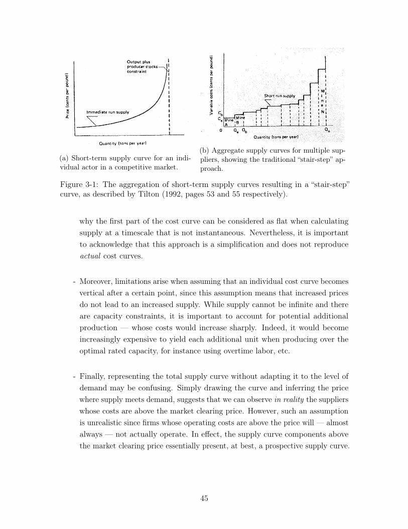
(a) Short-term supply curve for an indi-vidual actor in a competitive market.

(b) Aggregate supply curves for multiple sup-pliers, showing the traditional “stair-step” ap-proach.

Figure 3-1: The aggregation of short-term supply curves resulting in a “stair-step”curve, as described by Tilton (1992, pages 53 and 55 respectively).

why the first part of the cost curve can be considered as flat when calculatingsupply at a timescale that is not instantaneous. Nevertheless, it is importantto acknowledge that this approach is a simplification and does not reproduceactual cost curves.

- Moreover, limitations arise when assuming that an individual cost curve becomesvertical after a certain point, since this assumption means that increased pricesdo not lead to an increased supply. While supply cannot be infinite and thereare capacity constraints, it is important to account for potential additionalproduction — whose costs would increase sharply. Indeed, it would becomeincreasingly expensive to yield each additional unit when producing over theoptimal rated capacity, for instance using overtime labor, etc.

- Finally, representing the total supply curve without adapting it to the level ofdemand may be confusing. Simply drawing the curve and inferring the pricewhere supply meets demand, suggests that we can observe in reality the supplierswhose costs are above the market clearing price. However, such an assumptionis unrealistic since firms whose operating costs are above the price will — almostalways — not actually operate. In effect, the supply curve components abovethe market clearing price essentially present, at best, a prospective supply curve.

45

3.1.3 Considerations about Market Clearing

Economic theory assumes that market-clearing will occur, and in particular thatthe aggregate supply will meet the aggregate demand at each period. The actualmechanism that takes place to ensure this market clearing, as well as the way onecan implement it in a market model, are questions that are not often addressed incommon studies1.

A characteristic of markets is that actors cannot fully coordinate at each period;for practicality reasons first, since it would be extremely hard to gather all producersor alternatively all consumers to achieve such a coordination. Another reason is dueto the very regulation of markets: suppliers are not allowed to collude and fix acollaborative price, nor are groups of consumers allowed to form cartels.

Tackling the issue of market clearing in market models, while incorporating botheconomic theory and the reality of the market, hence becomes challenging. The m:5model has been built to address this issue of market clearing by using the notion ofa “market-maker” — as observed for precious metals for instance — that mediatestrades between consumers and suppliers, and computes the “fair” price consideringthe balance of current material offers and supplies. While this mechanism usuallytakes place on a daily basis with instantaneous supply and demand values, the modelassumes that, on a quarterly basis, the market-maker can infer the aggregate “real”supply and demand curves, and fix a resulting price. Section 3.2.2 will address thisnotion in more details.

3.2 Description of the Model

The m:5 model has been implemented as a spreadsheet model in Microsoft Excel®

for flexibility and transparency. For the purpose of simplifying this stage of modeldevelopment, demand is treated as exogenous, although there is no structural limitationto incorporating a full-blown demand model in the future. In order to add a certaindegree of price responsiveness to simulated demand, these “exogenous” demands canbe made price sensitive by setting a non-zero price elasticity in the model inputs for aparticular consumption sector. With demand trends and a set of inputs describingsources of supply (i.e., mines, their production economics, and their production

1There is however a formal domain, referred to as the study of the “microstructure” of a market,that studies these mechanisms. As acknowledged by Cohen et al. (1981), this field has been initiatedby the work of Stigler (1964) and the term itself has been later introduced by Garman (1976).

46

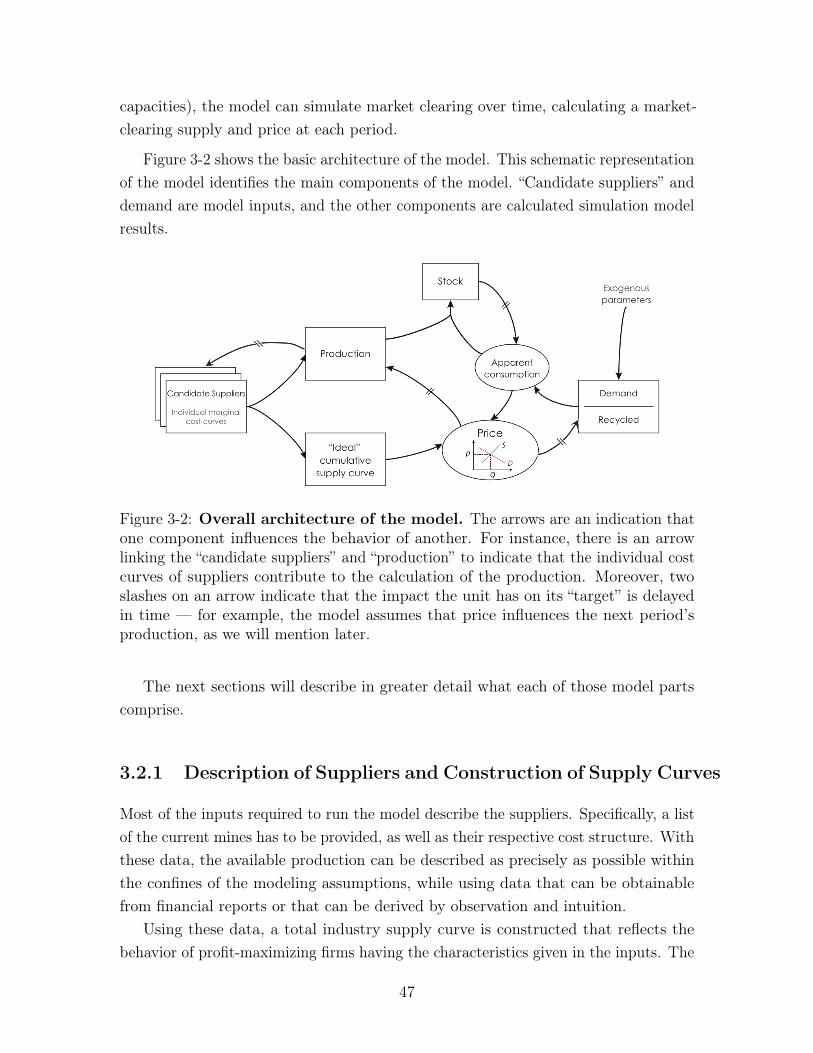
capacities), the model can simulate market clearing over time, calculating a market-clearing supply and price at each period.

Figure 3-2 shows the basic architecture of the model. This schematic representationof the model identifies the main components of the model. “Candidate suppliers” anddemand are model inputs, and the other components are calculated simulation modelresults.

Figure 3-2: Overall architecture of the model. The arrows are an indication thatone component influences the behavior of another. For instance, there is an arrowlinking the “candidate suppliers” and “production” to indicate that the individual costcurves of suppliers contribute to the calculation of the production. Moreover, twoslashes on an arrow indicate that the impact the unit has on its “target” is delayedin time — for example, the model assumes that price influences the next period’sproduction, as we will mention later.

The next sections will describe in greater detail what each of those model partscomprise.

3.2.1 Description of Suppliers and Construction of Supply Curves

Most of the inputs required to run the model describe the suppliers. Specifically, a listof the current mines has to be provided, as well as their respective cost structure. Withthese data, the available production can be described as precisely as possible withinthe confines of the modeling assumptions, while using data that can be obtainablefrom financial reports or that can be derived by observation and intuition.

Using these data, a total industry supply curve is constructed that reflects thebehavior of profit-maximizing firms having the characteristics given in the inputs. The

47

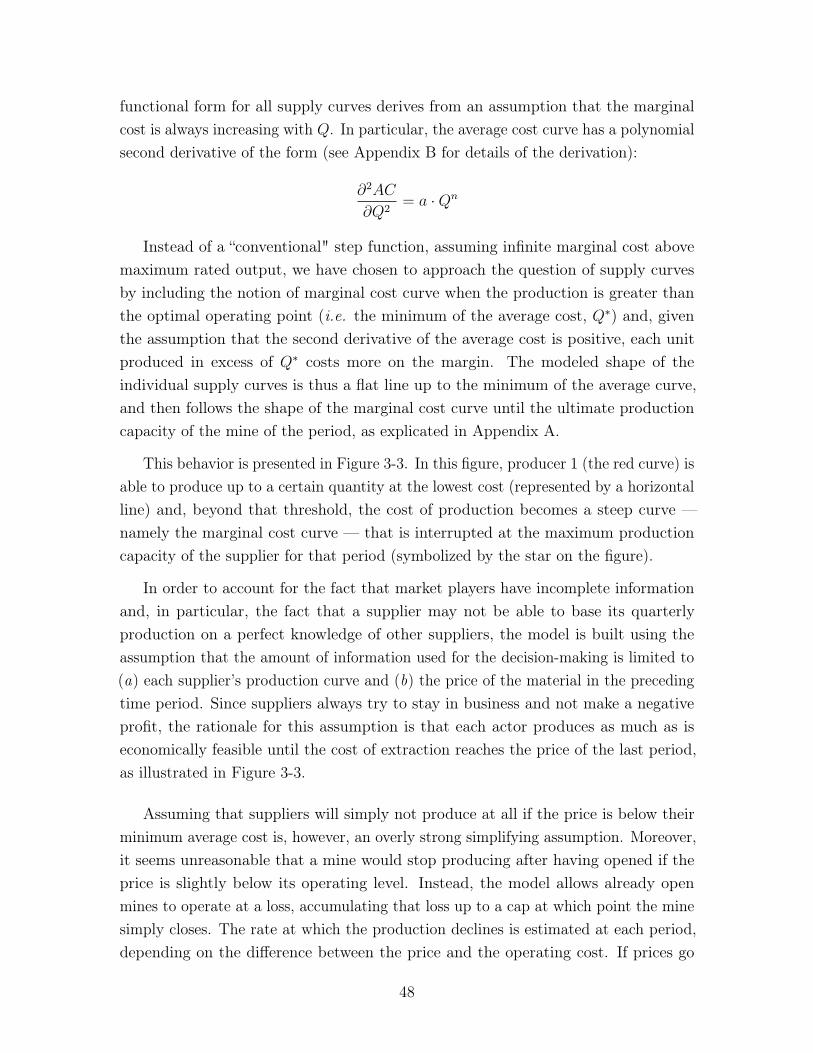
functional form for all supply curves derives from an assumption that the marginalcost is always increasing with Q. In particular, the average cost curve has a polynomialsecond derivative of the form (see Appendix B for details of the derivation):

@2AC

@Q2= a ·Qn

Instead of a “conventional" step function, assuming infinite marginal cost abovemaximum rated output, we have chosen to approach the question of supply curvesby including the notion of marginal cost curve when the production is greater thanthe optimal operating point (i.e. the minimum of the average cost, Q⇤) and, giventhe assumption that the second derivative of the average cost is positive, each unitproduced in excess of Q⇤ costs more on the margin. The modeled shape of theindividual supply curves is thus a flat line up to the minimum of the average curve,and then follows the shape of the marginal cost curve until the ultimate productioncapacity of the mine of the period, as explicated in Appendix A.

This behavior is presented in Figure 3-3. In this figure, producer 1 (the red curve) isable to produce up to a certain quantity at the lowest cost (represented by a horizontalline) and, beyond that threshold, the cost of production becomes a steep curve —namely the marginal cost curve — that is interrupted at the maximum productioncapacity of the supplier for that period (symbolized by the star on the figure).

In order to account for the fact that market players have incomplete informationand, in particular, the fact that a supplier may not be able to base its quarterlyproduction on a perfect knowledge of other suppliers, the model is built using theassumption that the amount of information used for the decision-making is limited to(a) each supplier’s production curve and (b) the price of the material in the precedingtime period. Since suppliers always try to stay in business and not make a negativeprofit, the rationale for this assumption is that each actor produces as much as iseconomically feasible until the cost of extraction reaches the price of the last period,as illustrated in Figure 3-3.

Assuming that suppliers will simply not produce at all if the price is below theirminimum average cost is, however, an overly strong simplifying assumption. Moreover,it seems unreasonable that a mine would stop producing after having opened if theprice is slightly below its operating level. Instead, the model allows already openmines to operate at a loss, accumulating that loss up to a cap at which point the minesimply closes. The rate at which the production declines is estimated at each period,depending on the difference between the price and the operating cost. If prices go

48

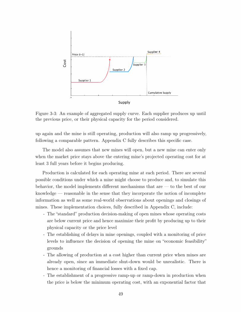
Figure 3-3: An example of aggregated supply curve. Each supplier produces up untilthe previous price, or their physical capacity for the period considered.

up again and the mine is still operating, production will also ramp up progressively,following a comparable pattern. Appendix C fully describes this specific case.

The model also assumes that new mines will open, but a new mine can enter onlywhen the market price stays above the entering mine’s projected operating cost for atleast 3 full years before it begins producing.

Production is calculated for each operating mine at each period. There are severalpossible conditions under which a mine might choose to produce and, to simulate thisbehavior, the model implements different mechanisms that are — to the best of ourknowledge — reasonable in the sense that they incorporate the notion of incompleteinformation as well as some real-world observations about openings and closings ofmines. These implementation choices, fully described in Appendix C, include:

- The “standard” production decision-making of open mines whose operating costsare below current price and hence maximize their profit by producing up to theirphysical capacity or the price level

- The establishing of delays in mine openings, coupled with a monitoring of pricelevels to influence the decision of opening the mine on “economic feasibility”grounds

- The allowing of production at a cost higher than current price when mines arealready open, since an immediate shut-down would be unrealistic. There ishence a monitoring of financial losses with a fixed cap.

- The establishment of a progressive ramp-up or ramp-down in production whenthe price is below the minimum operating cost, with an exponential factor that

49

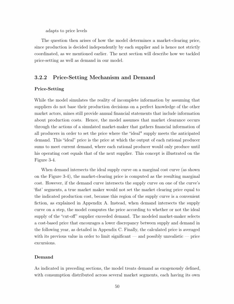
adapts to price levels

The question then arises of how the model determines a market-clearing price,since production is decided independently by each supplier and is hence not strictlycoordinated, as we mentioned earlier. The next section will describe how we tackledprice-setting as well as demand in our model.

3.2.2 Price-Setting Mechanism and Demand

Price-Setting

While the model simulates the reality of incomplete information by assuming thatsuppliers do not base their production decisions on a perfect knowledge of the othermarket actors, mines still provide annual financial statements that include informationabout production costs. Hence, the model assumes that market clearance occursthrough the actions of a simulated market-maker that gathers financial information ofall producers in order to set the price where the “ideal" supply meets the anticipateddemand. This “ideal” price is the price at which the output of each rational producersums to meet current demand, where each rational producer would only produce untilhis operating cost equals that of the next supplier. This concept is illustrated on theFigure 3-4.

When demand intersects the ideal supply curve on a marginal cost curve (as shownon the Figure 3-4), the market-clearing price is computed as the resulting marginalcost. However, if the demand curve intersects the supply curve on one of the curve’s‘flat’ segments, a true market maker would not set the market clearing price equal tothe indicated production cost, because this region of the supply curve is a convenientfiction, as explained in Appendix A. Instead, when demand intersects the supplycurve on a step, the model computes the price according to whether or not the idealsupply of the “cut-off” supplier exceeded demand. The modeled market-maker selectsa cost-based price that encourages a lower discrepancy between supply and demand inthe following year, as detailed in Appendix C. Finally, the calculated price is averagedwith its previous value in order to limit significant — and possibly unrealistic — priceexcursions.

Demand

As indicated in preceding sections, the model treats demand as exogenously defined,with consumption distributed across several market segments, each having its own

50

Figure 3-4: The price is set by the market-maker where the demand meets the “ideal"supply curve.

annual growth rate.

In order to consider the effects of differential responses to price excursions acrossthese segments, each consumption sector can be assigned a characteristic price elasticity,which imparts a limited price responsiveness to the overall sectorial growth in eachperiod. Appendix D will describe in greater detail how we accounted for elasticity.

The functional form of the supply curves — in particular the stability conventionleading to their “flat part” — combined with both incompleteness of information andlimited demand sensitivity, inevitably results in a discrepancy between supply anddemand, which the model treats by the creation of a stock. The next section describeshow stock is handled, as well as how mines evolve dynamically.

3.2.3 Stock and Mine Dynamics

Because of incomplete information and constraints on coordination, suppliers tendto produce a quantity that may not be strategically optimal to match demand. Inparticular, a profit-maximizing firm will operate at the output level where its marginalcost of production equals the market price, instead of stopping where their cost reachesthe level of the next supplier. When the production exceeds its “ideal” level (indicatedon Figure 3-4) we assign the resulting production imbalance to a running stock in the

51

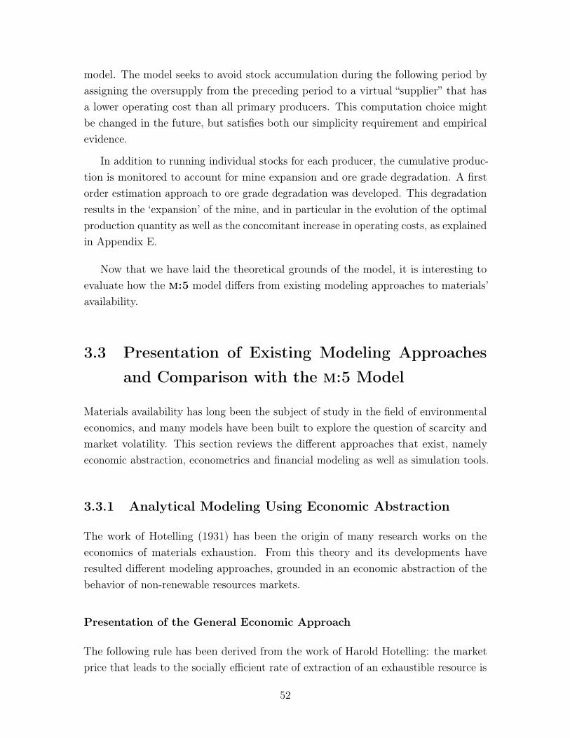
model. The model seeks to avoid stock accumulation during the following period byassigning the oversupply from the preceding period to a virtual “supplier” that hasa lower operating cost than all primary producers. This computation choice mightbe changed in the future, but satisfies both our simplicity requirement and empiricalevidence.

In addition to running individual stocks for each producer, the cumulative produc-tion is monitored to account for mine expansion and ore grade degradation. A firstorder estimation approach to ore grade degradation was developed. This degradationresults in the ‘expansion’ of the mine, and in particular in the evolution of the optimalproduction quantity as well as the concomitant increase in operating costs, as explainedin Appendix E.

Now that we have laid the theoretical grounds of the model, it is interesting toevaluate how the m:5 model differs from existing modeling approaches to materials’availability.

3.3 Presentation of Existing Modeling Approachesand Comparison with the m:5 Model

Materials availability has long been the subject of study in the field of environmentaleconomics, and many models have been built to explore the question of scarcity andmarket volatility. This section reviews the different approaches that exist, namelyeconomic abstraction, econometrics and financial modeling as well as simulation tools.

3.3.1 Analytical Modeling Using Economic Abstraction

The work of Hotelling (1931) has been the origin of many research works on theeconomics of materials exhaustion. From this theory and its developments haveresulted different modeling approaches, grounded in an economic abstraction of thebehavior of non-renewable resources markets.

Presentation of the General Economic Approach

The following rule has been derived from the work of Harold Hotelling: the marketprice that leads to the socially efficient rate of extraction of an exhaustible resource is

52

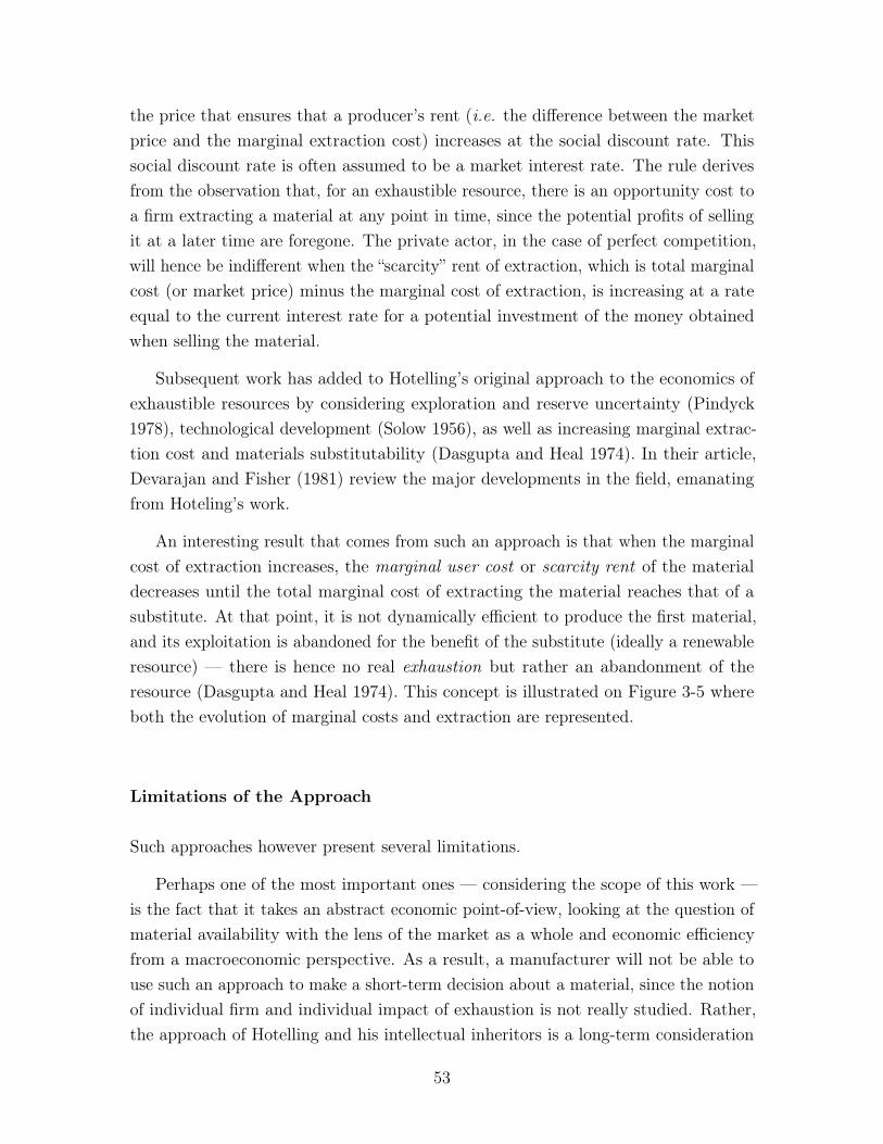
the price that ensures that a producer’s rent (i.e. the difference between the marketprice and the marginal extraction cost) increases at the social discount rate. Thissocial discount rate is often assumed to be a market interest rate. The rule derivesfrom the observation that, for an exhaustible resource, there is an opportunity cost toa firm extracting a material at any point in time, since the potential profits of sellingit at a later time are foregone. The private actor, in the case of perfect competition,will hence be indifferent when the “scarcity” rent of extraction, which is total marginalcost (or market price) minus the marginal cost of extraction, is increasing at a rateequal to the current interest rate for a potential investment of the money obtainedwhen selling the material.

Subsequent work has added to Hotelling’s original approach to the economics ofexhaustible resources by considering exploration and reserve uncertainty (Pindyck1978), technological development (Solow 1956), as well as increasing marginal extrac-tion cost and materials substitutability (Dasgupta and Heal 1974). In their article,Devarajan and Fisher (1981) review the major developments in the field, emanatingfrom Hoteling’s work.

An interesting result that comes from such an approach is that when the marginalcost of extraction increases, the marginal user cost or scarcity rent of the materialdecreases until the total marginal cost of extracting the material reaches that of asubstitute. At that point, it is not dynamically efficient to produce the first material,and its exploitation is abandoned for the benefit of the substitute (ideally a renewableresource) — there is hence no real exhaustion but rather an abandonment of theresource (Dasgupta and Heal 1974). This concept is illustrated on Figure 3-5 whereboth the evolution of marginal costs and extraction are represented.

Limitations of the Approach

Such approaches however present several limitations.

Perhaps one of the most important ones — considering the scope of this work —is the fact that it takes an abstract economic point-of-view, looking at the question ofmaterial availability with the lens of the market as a whole and economic efficiencyfrom a macroeconomic perspective. As a result, a manufacturer will not be able touse such an approach to make a short-term decision about a material, since the notionof individual firm and individual impact of exhaustion is not really studied. Rather,the approach of Hotelling and his intellectual inheritors is a long-term consideration

53

Time

Mar

gina

l Cos

t ($

/uni

t)

Total Marginal Cost

Margi

nal E

xtra

ction

Cos

t

Aband

onment of resource 1

Mar

gina

l Use

r C

ost

Resource 1 Resource 2

(a) Evolution of the marginal costs with time, when switchingfrom resource 1 (non-renewable) to resource 2 (renewable).

Time

Extr

acti

on /

Con

sum

pti

on

Consumption of resource 2

Aband

onment of resource 1

Extraction of resource 1

(b) Evolution of extraction and consumption with time, whenswitching from resource 1 (non-renewable) to resource 2 (renew-able).

Figure 3-5: The case of a non-renewable resource with an increasing marginal cost ofextraction, based on the theory developed by Dasgupta and Heal (1974).

54

based on “socially optimal extraction”, the “known” reserves for the material, and theaggregate marginal extraction cost.

Other limitations come from the adopted idealized vision of the market. Whileauthors such as Hotelling do consider the case of monopolies, other market imperfec-tions — incompleteness of information, exogenous disruptive events like conflicts orstrikes, externalities, poorly defined property rights etc. — are not usually explicitlyconsidered, which results in an assessment that does not encompass the whole pictureof the market. While it is interesting to develop this type of approach in order toframe theories about non-renewable resources, it is less relevant for a manufacturerthat needs a criticality-assessment in the short-term that considers as many criticalitysources as possible, in particular market imperfections.

Comparison of Such Approaches with the m:5 Model

The m:5 model as described in Section 3.1 differs from economic abstraction approachesby providing a tool that focuses decisions and strategies at the firm-level, both onthe supply-side and on the demand-side of the materials markets. Moreover, thetimescale considered is significantly different, since the abstract economics approachesdescribed above tend to focus on the long run, whereas the model developed duringthis work emphasizes the short-term — while still incorporating medium- to long-termconsiderations such as depletion and mine expansions.

The m:5 model is also shaped to be used by an individual decision-maker that canrefine the outputs of the model by implementing different demand scenarios; conversely,approaches grounded on an economic abstraction of markets consider the market as awhole and not the specific events leading to the abandonment of a resource, but ratherits inevitableness because of aggregate cost and finite crustal abundance. This focusderives from the desire to develop a tool that informs individual firm decision-making,which is both short-term and typically contingent upon an uncertain future.

The construction of the short-term supply curves in the m:5 model has beengrounded in standard economic theory, since much of the behavior of individualmines can be treated through conventional microeconomic arguments about profitmaximizing behavior, particularly the way in which pricing signals influence productiondecisions.

55

3.3.2 Financial-Based Modeling Approaches

The financial modeling-based approach is one that is often used by consulting firmsand some manufacturers. Instead of reliance upon economic theory to frame themodel, it employs econometric regressions of financial data to infer future demandand supply.

Presentation of the Financial Models

Mines prepare annual financial reports to present their operating results — includingtheir annual production and their operating cost — which is the main source of datafor financial models. Assuming that firm production decisions are based upon cashflow recovery, these econometric models aggregate the known capacities of existing andprospective mines, ordering them from lowest to highest operation cost to generate anindustry supply curve. Then, using demand forecasts, these models set the price levelusing the estimated industry supply curve to find where the level of industry outputfulfills forecast demand.

The timeframe considered in these approaches is very short, usually spanning fromone to four years. Supply and demand data are gathered on a yearly or bi-annual basis.Usually, a regression of either supply or demand is then run on different parameters— and in particular market price. The equilibrium point of price and output is theninferred from the other curve, so that forecasted supply can meet this consumptiontarget. It is hence a short-term approach.

These financial models are particularly useful in revealing price cycles and trends,as well as the effect of exploration or technological changes on markets, by studyinghistorical data and inferring relevant drivers and parameters (Labys, Lesourd, andBadillo 1998).

Limitations of the Approach

Financial-based models present several limitations that are different from those citedpreviously for models based on economic abstraction.

On the one hand, they are largely grounded in financial reporting data, evaluatingdemand on the one hand and supply on the other. This approach gets around theso-called “identification problem” (Koopmans 1949) when using regression to modelsupply and demand, since there is nothing in the historical data that can distinguishbetween the two — there is, in effect, only one observation than can be made which is

56

simultaneously demand and supply. The regression approach, therefore, usually relieson the very important assumption that supply and demand can be independentlydetermined and ignores potential interactions and dynamics2. In particular, demandis calculated based on historical trends of given parameters, independently from thequestion of price levels or supply constraints.

On the other hand, a regression model fundamentally assumes that the future willbe similar to the past. Hence, structural changes in the market deriving for instancefrom technological discovery, restructuring of consumer demand, or fundamentalincome effects, are not formally accounted for in the model, unless specifically treatedin the formulation — which requires technical insights that most financially-focusedanalysts are unlikely to have. The short-term aspect of such assessments thus providesgood insight when a decision needs to be made very quickly, but this limits thevisibility for a manufacturer that would like to study different scenarios and have abetter sense of medium-term market behaviors. An example would be that of a firmthat is planning on launching a new technology and would need the 10 to 15 yearsprojection of the market in order to verify whether the supply for the required materialis sufficiently well established to sustain a mass development of the technology, or not.The insights a financial model would provide in such a case would not incorporateeither the “disruptive” aspect of the demand pattern or the longer-term effect of thisincrease in demand.

Finally, the scope of the projections can sometimes be more tuned towards supplyactors, and in particular the decision for price is based on the financial data of thedifferent mines. Moreover, the way in which regression on demand is performeddepends on the modeler’s choice. In particular, demand aggregation for the differentdemand sectors can be done either prior to any regression, hence what is considered isthe total ‘consumption’ for the material; or regression can be performed for each sectorindependently and then the curves aggregated. While the second case may providemanufacturers with useful insight so as to how specific structural characteristics ofdemand may influence the market, it can be much harder to identify which sector hasa structural impact in the first case. Hence, from a manufacturer perspective, it canbe challenging to extract sector-level information to inform better decisions, while thefact that different sectors can behave differently can actually have a very significantimpact on the market, as will be discussed later in Section 4.2.2.

2There are very sophisticated techniques that are used to solve this issue — such as regressionmodels of simultaneous equations (see, for instance, Kmenta and Gilbert 1968) — but their complexitytends to limit their applicability in the real world.

57

Comparison of Such Approaches with the m:5 Model

In essence, a financial model will be similar to the modeling approach that has beenadopted in this work, since they both can be characterized as supply-demand models.In particular, the price is set at a level high enough to enable the last producer tooperate at a “reasonable” cost — namely at a cost that allows him to recover his totalcost.

Several aspects of financial models differ from this work’s approach, however. Thefirst one is that the timeframes within which the models work are different, since them:5 model aims at projecting supply and price sufficiently far out in time — about15 years — so that manufacturers can get a better picture of the market evolutionand make better-informed design and production decisions.

Another conceptual difference between the two approaches is that financial modelsdo not account for the interactions between supply and demand, nor do they adjustdemand to price levels and supply evolutions. Conversely, the supply-demand m:5model has been built so that demand would be sensitive to price evolutions, and henceindirectly to supply. The supply-demand interaction is also implemented in the m:5model via the establishment of a stock, arising when there is a discrepancy betweensupply and demand levels, and affecting the price by changing the shape of the supplycurve.

Hence the m:5 model is similar in essence to financial models, but adopts the pointof view of an individual firm or demand sector in order to devise demand decisionsthat are sustainable on the current market.

3.3.3 Simulation Tools: the Example of System DynamicsModeling

Finally, different types of simulation tools have been developed to look at materialsavailability with a dynamics perspective. These methods, and in particular systemdynamics models, are very comprehensive in that they aim at representing a complexsystem by using a system of interdependent non-linear first order differential equations.These systems are reduced to difference equations, which are then used as the basis forsimulation models that develop system behavior for a variety of initial and operatingconditions.

58

Presentation of System Dynamics Models

System dynamics models are particularly efficient when it comes to modeling thebehavior of inhomogeneous actors, as well as implementing time delays. The notion offeedback is also of great importance, and such models work with influence relationshipsbetween systems — for instance for recycling as a secondary supply stream. Inparticular, Alonso from the Materials Systems Laboratory at MIT developed a systemdynamics model for the platinum market (Alonso 2010) showing that changes inrecycling rates, resulting either from market forces or extra-market policies, cansignificantly influence market prices in materials markets subject to supply pressures.The work by Urbance of the Materials Systems Laboratory (Urbance 2001; Urbance etal. 2002) used a systems dynamics model to study the responsiveness of the magnesiumsupply chain to changes in automotive demand. The study revealed the dominantinfluence of barriers to entry — deriving from the technical and economic structure ofthe magnesium die casting industry — upon the expansion potential for the structuralmagnesium market overall.

The price-setting mechanism in the model by Alonso (2010), as well as other systemdynamics models, is driven by inventory coverage. More specifically, it is assumedthat a market-maker ensures liquidity on the market by selling and buying from aninventory in order to set the price at the level where the producers willingness-to-acceptis equal to the consumers willingness-to-pay. More specifically, the pricing mechanismformally examines the size of this inventory coverage, and adjusts prices according tothe simulated level of coverage as compared to a targeted level of coverage.

Limitations of the Approach

System dynamics models are often very thorough in their description of the market —a large amount of data is collected in order to describe as accurately as possible thebehavior of each individual actor in the market. As a result, the resources required togather enough data for such a model are extremely large. In many cases, it could takeseveral person-years of effort to gather enough information about supply, demand,recycling and speculation in order to accurately describe the market for one givenmaterial. Such an approach is incredibly time- and resource-intensive and cannotalways be used by manufacturers that need a quick assessment of market behaviorfor several materials. While it provides great insights on the market as a whole andenables the user to keep track of the different flows over time, the amount of effortrequired to build it and have it running is very large.

59

Moreover, system dynamics models frequently rely on modeling ‘fictions’ thatare elaborated by the model creator, such as the notion of “inventory coverage”, ormeasures of “willingness of an actor to make a specific decision”. Such fictions are notgrounded in reality and, while proxies can be developed, have no real either physicalor analytical analog. Hence, a third-party user might treat the model as a “black-box”tool, which lessens its effectiveness. A model that instead relies on available andreported data as well as uses generally-accepted theoretical constructs in a transparentmanner, offers a better understanding of its operations and, thus, of its results.

Comparison of Such Approaches with the Model Presented

When building the m:5 model, the intent was to implement a sufficient amount ofinformation about the market so as to accurately capture structural characteristics,while keeping it sufficiently simple and flexible in order for a manufacturer to easilyswitch from one material to another, and run insightful analyses without spendingtoo many resources to do so.

The m:5 model hence differs from system dynamics approaches by using a lessdata-intensive approach to materials markets; the downside of such an approach isthat it inherently reduces the accuracy of the modeling by limiting the amount ofprecision put into the model. Instead of requiring a full description of all the actors onthe market, the m:5 model only requires a list of suppliers with some financial datain order to describe the supply curve, but the latter has the same functional formfor each actor, even though it is parametrizable. However, this loss of accuracy is animplementation-specific design feature. If the analyst wants to increase the resolutionpower of the m:5 model, it is possible to do so by simply expanding its implementationthrough increased data. On the other hand, this design flexibility cannot be foundin system dynamics model, since the calculations are not transparent. For instance,there is no data that can reveal “inventory coverage” or other pseudo-metrics used bymodelers to describe actions.

Another difference in the system dynamics approach is the way inventory isconsidered. In the case of system dynamics models, inventory is what ultimatelysets the price, using the rationale that, if the inventory is too low, the price shouldincrease to provide a sufficient incentive for producers to enter the market and producemore, and vice versa. In the supply-demand model developed for this work however,inventory is merely an instrument for managing period-to-period imbalances in supplyand demand, and is not the dominant factor in setting the market clearing price.

60

While system dynamics models are very thorough and powerful tools that com-prehensively capture the complexity of materials markets and model the dynamicinteractions between supply, demand and price, they require a very detailed descriptionof all the individual components of the market that are endogenous to the model.As a result, the data and resources required are too high to be gathered in a timelyfashion for many different materials, putting real limits on the ability of an individualfirm to make strategic decisions across a broad spectrum of materials.

This section reviewed the existing modeling methods that tackle the question ofmaterials availability. The supply-demand model that has been developed is aimedat tackling the gaps we have identified in this section, and at providing a simple andgeneralizable tool, easily parametrizable by a manufacturer and requiring few inputs,yet still capturing the notion of market dynamics and imperfections. The followingsection will detail the different trade-offs that have been made when constructing them:5 model, in order to reach the desired level of precision while limiting the effortrequired to reach it.

3.4 Specifics of the m:5 Model and Applicability

This section presents the specifics about how a user can use the m:5 model to customizeit for the materials market of interest, as well as to assess alternative demand scenariosand policy strategies. While Section 3.1 describes the theory behind the m:5 model,here we demonstrate how it can be used in practice, as well as present the type ofquestion it can or cannot answer given its limitations and assumptions.

3.4.1 A User “Manual” for the m:5 Model

This section presents the different actions a user can perform with the model, in orderto implement different scenarios and compare their relative impact on the market. Inparticular, it describes what can be specified in the user inputs and how structuralchanges in the market — whether in the demand or the supply side — can be translatedinto parameter changes in the model.

61

Interface with the Supply Side

In the m:5 model, the list of suppliers — described using a limited set of financialdata at the desired starting point of the simulation — is defined as an input. It is thislist that makes the model specific to a given material market, since it describes thecurrent (and possibly expected) market players.

While the general shape of the supply curve is set by modeling assumptions basedon economic theory and a desire to limit the amount of information needed to run themodel, the actual parameters of the supply curve may be specified by the user.

The inputs required to describe a supplier are listed below, and fully described inAppendices A, B and E:

- Q⇤i

, the initial optimal production quantity. It is the quantity that the mineshould be producing at a given period, in order to operate at its lowest averagecost.

- A⇤i

, the initial minimum average cost of production. It is the point wherethe average cost curve and the marginal cost curve cross, and the resultingproduction is Q⇤

i

.- a, the multiplicative factor of the second derivative of the average cost function.

It is a scaling factor.- n, the polynomial exponent of the second derivative of the average cost curve.

It is possible to change it to affect the steepness of the marginal cost curve —hence allowing for more or less supply above the “optimal” production point,as explained in Section 3.2. Adjustments to this parameter could be used, forinstance, to compare the effect of a more or a less stringent environmentalmining regulation: the steeper the curve, the more stringent the policy (i.e., asteeper curve indicates that it gets increasingly more expensive to produce eachadditional unit).

- f1 and f2, the two interpolation parameters to invert the marginal cost curve.While they are mainly calculation parameters, f2 also is the multiplicative factorof Q⇤ that is the upper limit of production at each period. For instance, iff2 = 2, then the mine cannot produce more than 2 ·Q⇤ at each period — due tophysical and operational constraints.

- ↵, the rate of decline of the ore grade. The higher it is, the more quickly the oregrade will degrade when the cumulative production increases.

- gi

and gmin

, the initial and minimum ore grades, respectively. In particular, gmin

constitutes the ore grade floor, in the sense that a lower ore grade would not beeconomically profitable to exploit for the mine.

- Ktot

, the expected total cumulative output of the mine. It is the ‘reserve’ of

62

resource that investors project when opening the mine.- ⌧

life

, the projected lifetime of the mine, as established by the investors whenopening the mine — it is used to allocate the investment costs over time.

- �, the capital invested initially in the mine, discounted for its expected lifetime.

Because m:5 is a spreadsheet model, the user can easily access the individualcalculations made to simulate supply and other outputs for each time period. As aresult, the user can implement a “supply disruption” scenario, where, without impairingthe overall behavior of the model, the user can choose to let a given mine either stopproducing for a given number of periods, or produce only a fixed amount for a givenperiod of time (simulating a quota).

Finally, the m:5 model can be used to simulate the opening of new mines. Ifpotential new actors are described on the inputs page, the model will add them to thelist of suppliers if the price is high enough that they can feasibly operate. The model,of course, considers that there will be a delay in the opening of a new mine, reflectingthe influence of risk aversion on the part of the new mine operator. If these conditionsare satisfied, the model will incorporate this new mine into the market supply, andoffers a assessment of the effect this additional supply source may have on the market.

Changes in Demand

One of the design choices made when building this modeling tool was to have demandexogenously defined. While a notion of feedback has been implemented via the useof price elasticity of demand, the underlying demand trend is defined by exogenousparameters — such as the growth rate and the price elasticity of each sector. Hencethe user of the model has the ability to refine a demand scenario and evaluate theconsequences of the different parameters on the simulation results.

A user can choose to have the demand calculated at each period following thefunctional form described in Appendix D. As constructed in the model, total demandhas been segmented into different sectors that can be independently described. Byproviding a growth rate, a seasonal factor, a price elasticity, and the demand segment’srelative share of the global demand at the initial point in time, a manufacturer candescribe an existing market and use growth forecasts for each sector in order to seethe impact of such a scenario on the existing market. Additionally, recycling hasbeen implemented in the m:5 model as an exogenous mechanism whose occurrence isspecific to each demand sector, characterized by the recovery rate and the averagelifetime of products within each sector.

63

Demand can also be described fully exogenously by using a direct forecast andusing this externally estimated scenario as a time series executed by the model. Thisoperating mode is particularly useful when a decision-maker has already developeda specific demand scenario and wants to see its impact on the market. This featureexists so as to allow for more sophisticated demand scenarios, since the currentimplementation of demand is fairly simplistic.

Other Actionable Levers

Besides direct interactions with the list of suppliers and the different demand sectors’parameters, the m:5 model offers other parametrizable calculation tools. Thesefeatures have been implemented for transparency and flexibility — the model makessome general assumptions about markets, but offers the possibility to change theseassumptions.

Opening and Closing of Mines: As described in Appendix C, the model allowsfor mines to operate at a loss, since it would not be realistic to completely shutdown the mine on the sole ground that the price just went below the minimumoperating cost of the mine. The moving financial loss is monitored over a periodof time that can be set by the user, and the overall loss acceptable before thecomplete shut-down of the facility is also a modeling parameter. Moreover,production ramps up and down according to an exponential factor ⌧ (definedin Appendix C), whose evolution, given the cumulative loss, can also be tunedby the user. As a component of the model’s simulation of the “opening” of anew mine, the length of the period during which the price should be above theprojected operating cost of a new mine can also be set by the user.

Price Elasticity of Demand: Appendix D describes how price elasticity of demandis used to implement the notion of supply-demand feedback. Because this calcu-lation depends upon a weighted average of past prices, the user can incorporateadditional refinement to each demand sector’s price sensitivity, by changing boththe weights of the moving average and its length.

Price-Setting and Production: The assumptions governing the behavior of themarket-maker can be modified by the user — in particular, the values used toadjust the price level if there is an under- or an over-supply can be changed.Moreover, while the production calculation currently allows producers to extractup to the minimum of (a) the price of the previous period or (b) their ultimate

64

physical capacity at that period, that decision-making can be changed by using,for instance, an expected price value. While these calculations are not fullyparametrized yet, they are easily accessible.

3.4.2 Assumptions and Resulting Simplifications of the m:5Model

This section presents the different simplifications that have been adopted during theimplementation of the model.

Exploration and Discovery

The current version of the m:5 model is deterministic. In particular, the list ofsuppliers — current and projected — is set by the user. A mechanism has beendevised so that the entrance of a new actor on the market is delayed in time andgrounded in the rationale that the operating and investment costs are recovered overa reasonable timeframe. While the decision of opening the mine is based on the pricelevel, it is deterministic in that only the listed suppliers may be in the market.

In reality, the market for non-renewable resources presents uncertainty, especiallywhen it comes to discovery. In his paper, Pindyck (1978) introduces the notion thatthe reserve base is variable. The m:5 model incorporates an idea of exploration, inthat each mine evolves with respect to its cumulative production; specifically (a) theore grade degrades at a certain rate (set by the user), (b) the production increaseswith time while (c) the cost of extraction slightly increases as well, but this process isdeterministic.

The scope of the model is to address the short- to medium-term question ofwhether a demand scenario is sustainable given the current supply sources. Because astochastic discovery and exploration process introduces considerable complexity, thesefeatures were not implemented in this version of the model. However, future work onthe model could incorporate the question of variability in discovery of new mines andexpansion of existing ones.

The Question of Stock and Investment

One of the main assumptions of the m:5 model lies in the way material stocks havebeen implemented. In m:5, stocks are a bookkeeping instrument to account for

65

oversupply or undersupply in any time period. When stocks are nonzero, the valueof the stock is currently treated as an additional supplier having the lowest cost ofall operating suppliers so that the stock accumulated at one period will be consumedin the next period. As a result, stock as it is handled for now affects the price byshifting the supply curve “to the right”, increasing the available supply on the marketand possibly lowering the price of the resource — conversely, an undersupply leads toan increase in price.

In reality, a more strategic handling of stocks takes place in the market. On theone hand, manufacturers may have an incentive to keep a certain level of inventory asa buffer to hedge against demand when prices for feedstocks are excessive. Similarly,producers themselves might keep a positive level of inventory that they can use tomanage variable or seasonal demand — it hence becomes a safety buffer. In thecurrent version of the model, this “running stock” is held constant for each actor, andit is not elastic to price levels.

Another aspect of stock is its influence on the behavior of a third class of actors inthe resource market, that of investors or speculators. In markets like precious metals,the high stakes and material values lead to the involvement of outside actors — suchas investors — that are neither direct consumers nor suppliers. By buying stock at lowprices and selling it when prices increase, these speculative investors add an additionalcomplexity to the market and influence price levels by acting either as consumers orproducers, depending on price levels.

Such behaviors will have an impact on price levels, and can either result in exacer-bated price excursions, or conversely in a reduced price volatility. For simplificationreasons, and in order to limit the amount of necessary input data, the current modelcan only implement these behaviors in a limited fashion. Indeed, a demand sector canbe created with an upward-sloping demand curve (i.e. a positive price elasticity). Yetthis approach does not capture the full scope of an investor’s behavior and furthermodeling efforts could be oriented towards implementing it in greater detail.

The Handling of Recycling

A related modeling simplification is that m:5 implements recycling as both exogenousand deterministic. a recovery rate and an average product lifetime are modeling inputparameters for each sector. The quantity recycled at each period is then determinedas a fixed percentage of the demand at time t

i

= t� product lifetime. This approachassumes that both the recovery rate and the product lifetime are certain, hence making

66

the recycling stream deterministic. The quantity recycled at each period is then addedto the stock value and gets consumed at the next period.

A more realistic perspective on recycling could incorporate uncertainty bothconcerning the rate and the lifetime of the products. Since recycling is determinedby demand sector, the model could be improved by using probabilistic distributionsaround the average values for recycling, rendering this simulation of the secondarystream stochastic, in closer accord with reality.

As was the case for stock, the amount of material that gets recycled at each periodmay be held so as to get sold when the prices are higher. Similarly, higher priceson the market may encourage a higher recycling rate. Hence, incorporating pricesensitivity when calculating the quantity of material recycled and sold may add someadditional realism in the model and make the estimate of price at each period moreaccurate.

Yet, even with these limitations, recycling still has an impact on the overall stabilityof the market, as we will see in Section 4.1.3.

3.4.3 What Types of Questions Can the m:5 Model Answer?

Based on the description of the model that has been given in Section 3.2 and on themodel assumptions and limitations listed in the previous paragraphs, this sectionprovides insights so as to what type of questions can be treated by the m:5 modeland the insights that can be gained from the use of such a model.

First, it is important to note that the model that has been developed does nothave a predictive purpose, but rather is a tool that enables the user to comparedifferent scenarios, evaluate their relative impact, and act on different market-levellevers. Rather than giving exact values for future prices and supply, the model aimsat warning the decision-maker when there is a risk with a large potential impact, fromthe point of view of the manufacturer. It can hence be seen as a tool that (a) flagsexcessive risks and (b) compares the relative impacts different scenarios and policiescan have on the market and on a manufacturer in particular.

In the rest of this section, we will provide some sample questions the model cananswer, considering its foundations and limitations, and given the actionable leversthat have been mentioned in Section 3.4.1.

67

Questions Relative to Supply

The m:5 model offers a great flexibility in the characterization of the suppliers. As aresult, several types of questions can be addressed via the use of the model. Someexamples are provided below.

Influence of Supply Structure: By changing the distribution of suppliers — theconcentration of supply, as well as the distribution of cost levels — the usercan compare the relative impact of different structural characteristics that canreflect real-world observations of evolutions of supply sources. Moreover, theeffects of mine openings or closings can be explored.

Impact of Supply Instability By imposing supply values for particular suppliersover a given period of time (for instance, forcing a supplier to not produce fornumber of years), the decision-maker can study the effect of such a disruptionon the price and the behavior of the market in the longer-term. When lookingat critical elements, supply disruptions may occur due to external events —conflicts, strikes, governmental strategies, etc. If there is an expected risk ofsuch supply disruption, it is possible for a manufacturer to see its relative impacton the market and hence help him devise a better-informed strategies in theface of these risks.

Effect of Mine Dynamics By allowing mines to expand with respect to their cu-mulative production and the resulting depletion of the ore grade, the user cananalyze the relative impact of mine maturation and aging has on the longer-termsupply for the material, since it depends on the actual production.

Questions Relative to Demand

By treating the demand as exogenous, the m:5 model allows for a large flexibilityin the implementation of demand scenarios. Several types of questions can hence beasked by a manufacture or a policy-maker; some are listed below:

Influence of Demand Structure Launching a new technology that uses a signif-icant amount of a given material means either creating a new demand sector,or increasing the demand of an existing sector. In both cases, projecting theresulting expected demand in the m:5 model will enable a decision-maker toevaluate whether the current state of supply can sustain the increase in demandor to project the point in time when demand becomes unsustainable.

68

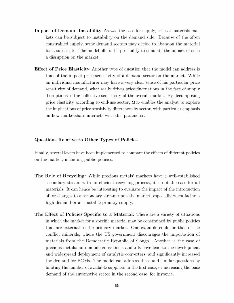
Impact of Demand Instability As was the case for supply, critical materials mar-kets can be subject to instability on the demand side. Because of the oftenconstrained supply, some demand sectors may decide to abandon the materialfor a substitute. The model offers the possibility to simulate the impact of sucha disruption on the market.

Effect of Price Elasticity Another type of question that the model can address isthat of the impact price sensitivity of a demand sector on the market. Whilean individual manufacturer may have a very clear sense of his particular pricesensitivity of demand, what really drives price fluctuations in the face of supplydisruptions is the collective sensitivity of the overall market. By decomposingprice elasticity according to end-use sector, m:5 enables the analyst to explorethe implications of price sensitivity differences by sector, with particular emphasison how marketshare interacts with this parameter.

Questions Relative to Other Types of Policies

Finally, several levers have been implemented to compare the effects of different policieson the market, including public policies.

The Role of Recycling: While precious metals’ markets have a well-establishedsecondary stream with an efficient recycling process, it is not the case for allmaterials. It can hence be interesting to evaluate the impact of the introductionof, or changes to a secondary stream upon the market, especially when facing ahigh demand or an unstable primary supply.

The Effect of Policies Specific to a Material: There are a variety of situationsin which the market for a specific material may be constrained by public policiesthat are external to the primary market. One example could be that of theconflict minerals, where the US government discourages the importation ofmaterials from the Democratic Republic of Congo. Another is the case ofprecious metals: automobile emissions standards have lead to the developmentand widespread deployment of catalytic converters, and significantly increasedthe demand for PGMs. The model can address these and similar questions bylimiting the number of available suppliers in the first case, or increasing the basedemand of the automotive sector in the second case, for instance.

69

The Impact of Environmental Mining Regulations: While critical materials’markets are not always well-regulated, it can be expected that more stringentmining standards will be imposed in the future. In particular, in the case ofREEs, the mining processes in China have put a high stress on the environment,and have recently been more stringently regulated (Situation and Policies ofChina’s Rare Earth Industry 2010). By changing the cost curve parameters, andin particular those of the marginal cost of extraction, the model user can addressthe question of relative impact of the policy on the stability of the market,since it directly implements the policy by changing the cost of extracting eachadditional unit.

70

Chapter 4

Results

This chapter presents insights that can be obtained through the use of the model, aswell as a discussion of what can be gained from the use of such a model and whatthe trade-offs are between how much effort has to be applying this type of tool andthe improvement it makes. Finally, the model and general observations of criticalmaterials markets are used to provide potential policy strategies to mitigate sometypes of material criticality.

4.1 Use of the Model to Illustrate Critical Materials’Markets Behaviors

This section presents results that have been obtained with the model to illustrate thebehavior of critical materials’ markets, and show how the m:5 model can capturesome characteristic dynamics of markets. In particular, the following paragraphs willaddress the use of m:5 to explore the structural characteristics of supply and demand,as well as the impact of different policies that have been mentioned in Section 3.4.3.

The inputs used for these analyses are fictional, yet loosely based on real preciousmetals markets and, in particular, the market for platinum.

4.1.1 Influence of Structural Characteristics of Supply

This section addresses issues of supply structure. Critical minerals markets arefrequently supply constrained, as presented in the second chapter of this thesis. It

71

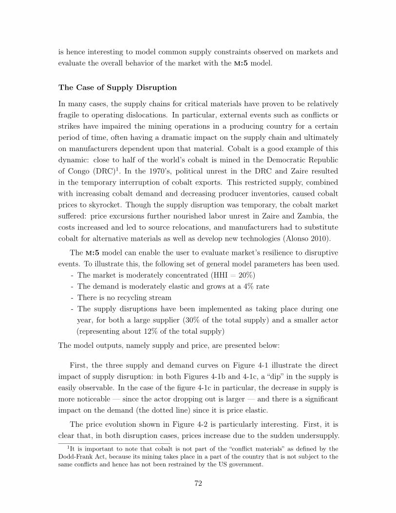
is hence interesting to model common supply constraints observed on markets andevaluate the overall behavior of the market with the m:5 model.

The Case of Supply Disruption

In many cases, the supply chains for critical materials have proven to be relativelyfragile to operating dislocations. In particular, external events such as conflicts orstrikes have impaired the mining operations in a producing country for a certainperiod of time, often having a dramatic impact on the supply chain and ultimatelyon manufacturers dependent upon that material. Cobalt is a good example of thisdynamic: close to half of the world’s cobalt is mined in the Democratic Republicof Congo (DRC)1. In the 1970’s, political unrest in the DRC and Zaire resultedin the temporary interruption of cobalt exports. This restricted supply, combinedwith increasing cobalt demand and decreasing producer inventories, caused cobaltprices to skyrocket. Though the supply disruption was temporary, the cobalt marketsuffered: price excursions further nourished labor unrest in Zaire and Zambia, thecosts increased and led to source relocations, and manufacturers had to substitutecobalt for alternative materials as well as develop new technologies (Alonso 2010).

The m:5 model can enable the user to evaluate market’s resilience to disruptiveevents. To illustrate this, the following set of general model parameters has been used.

- The market is moderately concentrated (HHI = 20%)- The demand is moderately elastic and grows at a 4% rate- There is no recycling stream- The supply disruptions have been implemented as taking place during one

year, for both a large supplier (30% of the total supply) and a smaller actor(representing about 12% of the total supply)

The model outputs, namely supply and price, are presented below:

First, the three supply and demand curves on Figure 4-1 illustrate the directimpact of supply disruption: in both Figures 4-1b and 4-1c, a “dip” in the supply iseasily observable. In the case of the figure 4-1c in particular, the decrease in supply ismore noticeable — since the actor dropping out is larger — and there is a significantimpact on the demand (the dotted line) since it is price elastic.

The price evolution shown in Figure 4-2 is particularly interesting. First, it isclear that, in both disruption cases, prices increase due to the sudden undersupply.

1It is important to note that cobalt is not part of the “conflict materials” as defined by theDodd-Frank Act, because its mining takes place in a part of the country that is not subject to thesame conflicts and hence has not been restrained by the US government.

72

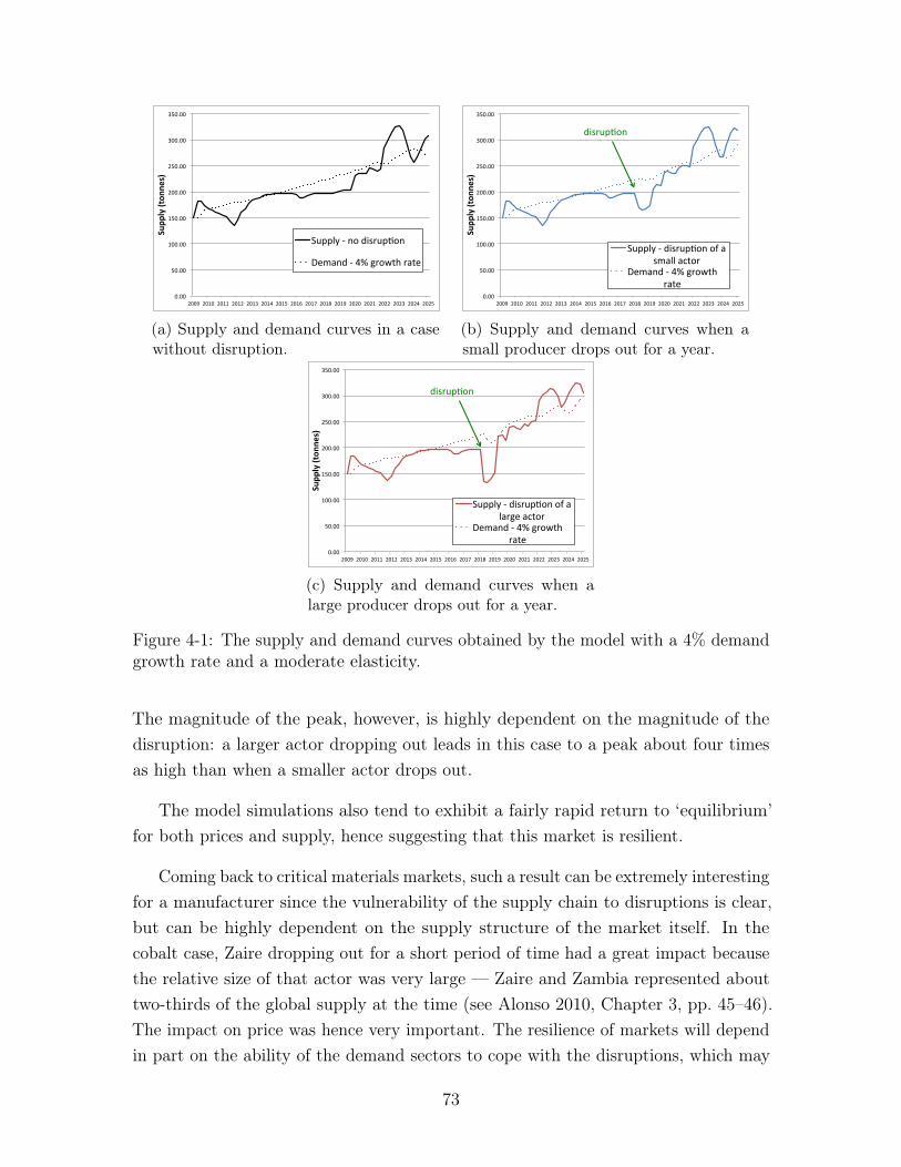
0.00#

50.00#

100.00#

150.00#

200.00#

250.00#

300.00#

350.00#

2009# 2010# 2011# 2012# 2013# 2014# 2015# 2016# 2017# 2018# 2019# 2020# 2021# 2022# 2023# 2024# 2025#

Supp

ly&(ton

nes)&

Supply#2#no#disrup9on#

Demand#2#4%#growth#rate#

(a) Supply and demand curves in a casewithout disruption.

0.00#

50.00#

100.00#

150.00#

200.00#

250.00#

300.00#

350.00#

2009# 2010# 2011# 2012# 2013# 2014# 2015# 2016# 2017# 2018# 2019# 2020# 2021# 2022# 2023# 2024# 2025#

Supp

ly&(ton

nes)&

Supply#2#disrup7on#of#a#small#actor#

Demand#2#4%#growth#rate#

disrup7on#

(b) Supply and demand curves when asmall producer drops out for a year.

0.00#

50.00#

100.00#

150.00#

200.00#

250.00#

300.00#

350.00#

2009# 2010# 2011# 2012# 2013# 2014# 2015# 2016# 2017# 2018# 2019# 2020# 2021# 2022# 2023# 2024# 2025#

Supp

ly&(ton

nes)&

Supply#2#disrup7on#of#a#large#actor#

Demand#2#4%#growth#rate#

disrup7on#

(c) Supply and demand curves when alarge producer drops out for a year.

Figure 4-1: The supply and demand curves obtained by the model with a 4% demandgrowth rate and a moderate elasticity.

The magnitude of the peak, however, is highly dependent on the magnitude of thedisruption: a larger actor dropping out leads in this case to a peak about four timesas high than when a smaller actor drops out.

The model simulations also tend to exhibit a fairly rapid return to ‘equilibrium’for both prices and supply, hence suggesting that this market is resilient.

Coming back to critical materials markets, such a result can be extremely interestingfor a manufacturer since the vulnerability of the supply chain to disruptions is clear,but can be highly dependent on the supply structure of the market itself. In thecobalt case, Zaire dropping out for a short period of time had a great impact becausethe relative size of that actor was very large — Zaire and Zambia represented abouttwo-thirds of the global supply at the time (see Alonso 2010, Chapter 3, pp. 45–46).The impact on price was hence very important. The resilience of markets will dependin part on the ability of the demand sectors to cope with the disruptions, which may

73

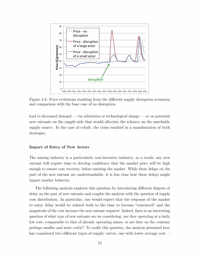
0"

10"

20"

30"

40"

50"

60"

70"

80"

90"

2009" 2010" 2011" 2012" 2013" 2014" 2015" 2016" 2017" 2018" 2019" 2020" 2021" 2022" 2023" 2024" 2025"

Price&($/grammes)&

Price"1"no"disrup8on"

Price"1"disrup8on"of"a"large"actor"

Price"1"disrup8on"of"a"small"actor"

disrup8on"

Figure 4-2: Price evolutions resulting from the different supply disruption scenarios,and comparison with the base case of no disruption.

lead to decreased demand — via substation or technological change — or on potentialnew entrants on the supply-side that would alleviate the reliance on the unreliablesupply source. In the case of cobalt, the crisis resulted in a manifestation of bothstrategies.

Impact of Entry of New Actors

The mining industry is a particularly cost-intensive industry; as a result, any newentrant will require time to develop confidence that the market price will be highenough to ensure cost recovery, before entering the market. While these delays on thepart of the new entrant are understandable, it is less clear how these delays mightimpact market behavior.

The following analysis explores this question by introducing different degrees ofdelay on the part of new entrants and couples the analysis with the question of supplycost distribution. In particular, one would expect that the response of the marketto entry delay would be related both to the time to become “convinced” and themagnitude of the cost increase the new entrant required. Indeed, there is an interestingquestion of what type of new entrants are we considering: are they operating at a fairlylow cost, comparable to that of already operating mines, or are they on the contraryperhaps smaller and more costly? To tackle this question, the analysis presented herehas considered two different types of supply curves, one with lower average cost —

74

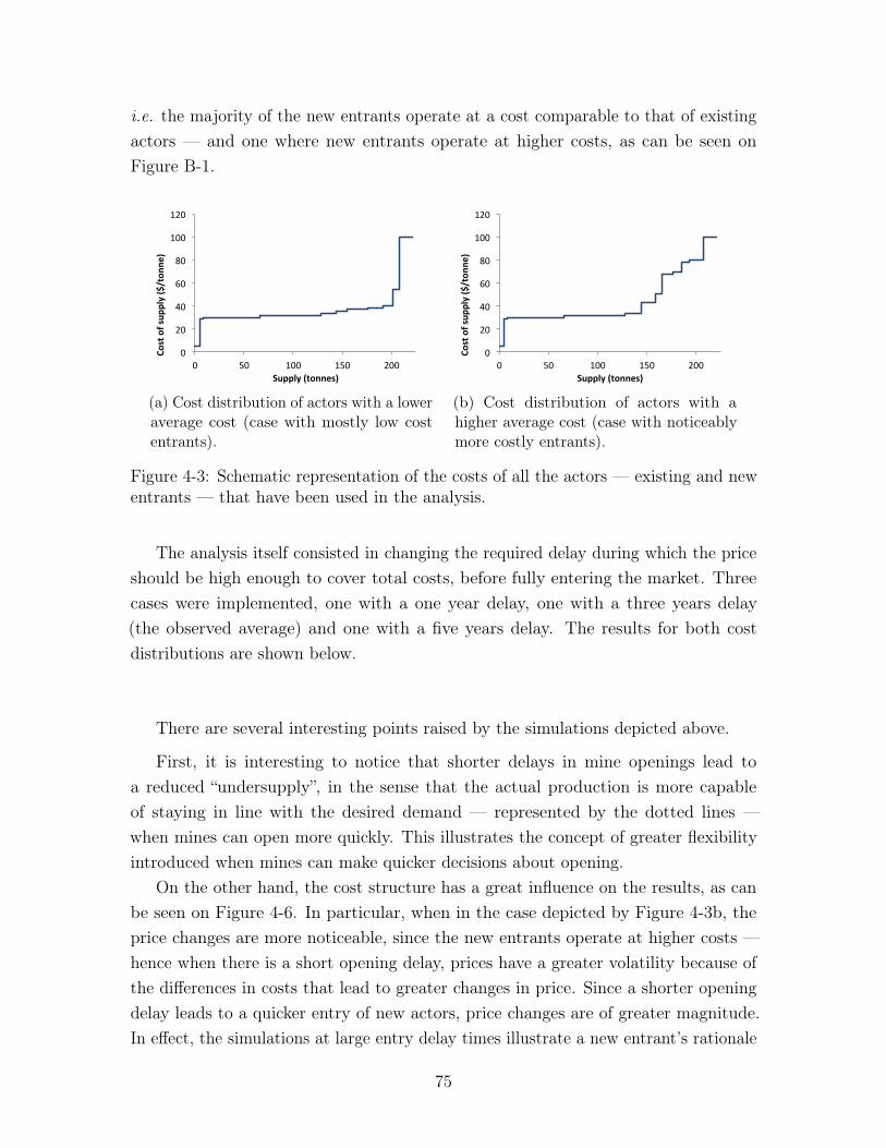
i.e. the majority of the new entrants operate at a cost comparable to that of existingactors — and one where new entrants operate at higher costs, as can be seen onFigure B-1.

0"

20"

40"

60"

80"

100"

120"

0" 50" 100" 150" 200"

Cost%of%sup

ply%($/ton

ne)%

Supply%(tonnes)%

(a) Cost distribution of actors with a loweraverage cost (case with mostly low costentrants).

0"

20"

40"

60"

80"

100"

120"

0" 50" 100" 150" 200"

Cost%of%sup

ply%($/ton

ne)%

Supply%(tonnes)%

(b) Cost distribution of actors with ahigher average cost (case with noticeablymore costly entrants).

Figure 4-3: Schematic representation of the costs of all the actors — existing and newentrants — that have been used in the analysis.

The analysis itself consisted in changing the required delay during which the priceshould be high enough to cover total costs, before fully entering the market. Threecases were implemented, one with a one year delay, one with a three years delay(the observed average) and one with a five years delay. The results for both costdistributions are shown below.

There are several interesting points raised by the simulations depicted above.

First, it is interesting to notice that shorter delays in mine openings lead toa reduced “undersupply”, in the sense that the actual production is more capableof staying in line with the desired demand — represented by the dotted lines —when mines can open more quickly. This illustrates the concept of greater flexibilityintroduced when mines can make quicker decisions about opening.

On the other hand, the cost structure has a great influence on the results, as canbe seen on Figure 4-6. In particular, when in the case depicted by Figure 4-3b, theprice changes are more noticeable, since the new entrants operate at higher costs —hence when there is a short opening delay, prices have a greater volatility because ofthe differences in costs that lead to greater changes in price. Since a shorter openingdelay leads to a quicker entry of new actors, price changes are of greater magnitude.In effect, the simulations at large entry delay times illustrate a new entrant’s rationale

75

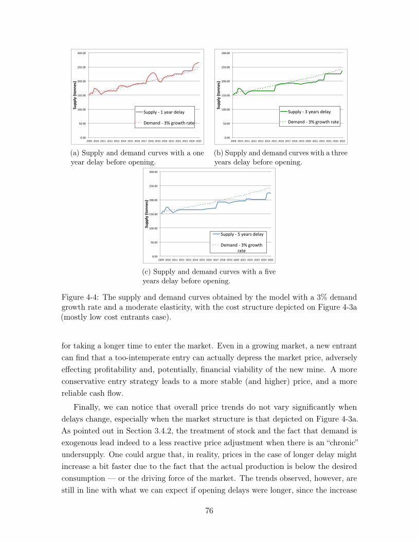
0.00#

50.00#

100.00#

150.00#

200.00#

250.00#

300.00#

2009# 2010# 2011# 2012# 2013# 2014# 2015# 2016# 2017# 2018# 2019# 2020# 2021# 2022# 2023# 2024# 2025#

Supp

ly&(ton

nes)&

Supply#2#1#year#delay#

Demand#2#3%#growth#rate#

(a) Supply and demand curves with a oneyear delay before opening.

0.00#

50.00#

100.00#

150.00#

200.00#

250.00#

300.00#

2009# 2010# 2011# 2012# 2013# 2014# 2015# 2016# 2017# 2018# 2019# 2020# 2021# 2022# 2023# 2024# 2025#

Supp

ly&(ton

nes)&

Supply#2#3#years#delay#

Demand#2#3%#growth#rate#

(b) Supply and demand curves with a threeyears delay before opening.

0.00#

50.00#

100.00#

150.00#

200.00#

250.00#

300.00#

2009# 2010# 2011# 2012# 2013# 2014# 2015# 2016# 2017# 2018# 2019# 2020# 2021# 2022# 2023# 2024# 2025#

Supp

ly&(ton

nes)&

Supply#2#5#years#delay#

Demand#2#3%#growth#rate#

(c) Supply and demand curves with a fiveyears delay before opening.

Figure 4-4: The supply and demand curves obtained by the model with a 3% demandgrowth rate and a moderate elasticity, with the cost structure depicted on Figure 4-3a(mostly low cost entrants case).

for taking a longer time to enter the market. Even in a growing market, a new entrantcan find that a too-intemperate entry can actually depress the market price, adverselyeffecting profitability and, potentially, financial viability of the new mine. A moreconservative entry strategy leads to a more stable (and higher) price, and a morereliable cash flow.

Finally, we can notice that overall price trends do not vary significantly whendelays change, especially when the market structure is that depicted on Figure 4-3a.As pointed out in Section 3.4.2, the treatment of stock and the fact that demand isexogenous lead indeed to a less reactive price adjustment when there is an “chronic”undersupply. One could argue that, in reality, prices in the case of longer delay mightincrease a bit faster due to the fact that the actual production is below the desiredconsumption — or the driving force of the market. The trends observed, however, arestill in line with what we can expect if opening delays were longer, since the increase

76

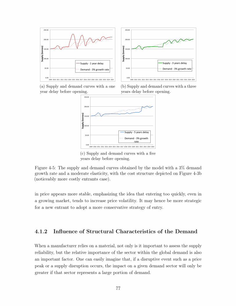
0.00#

50.00#

100.00#

150.00#

200.00#

250.00#

2009# 2010# 2011# 2012# 2013# 2014# 2015# 2016# 2017# 2018# 2019# 2020# 2021# 2022# 2023# 2024# 2025#

Supp

ly&(ton

nes)&

Supply#2#1#year#delay#

Demand#2#3%#growth#rate#

(a) Supply and demand curves with a oneyear delay before opening.

0.00#

50.00#

100.00#

150.00#

200.00#

250.00#

2009# 2010# 2011# 2012# 2013# 2014# 2015# 2016# 2017# 2018# 2019# 2020# 2021# 2022# 2023# 2024# 2025#

Supp

ly&(ton

nes)&

Supply#2#3#years#delay#

Demand#2#3%#growth#rate#

(b) Supply and demand curves with a threeyears delay before opening.

0.00#

50.00#

100.00#

150.00#

200.00#

250.00#

2009# 2010# 2011# 2012# 2013# 2014# 2015# 2016# 2017# 2018# 2019# 2020# 2021# 2022# 2023# 2024# 2025#

Supp

ly&(ton

nes)&

Supply#2#5#years#delay#

Demand#2#3%#growth#rate#

(c) Supply and demand curves with a fiveyears delay before opening.

Figure 4-5: The supply and demand curves obtained by the model with a 3% demandgrowth rate and a moderate elasticity, with the cost structure depicted on Figure 4-3b(noticeably more costly entrants case).

in price appears more stable, emphasizing the idea that entering too quickly, even ina growing market, tends to increase price volatility. It may hence be more strategicfor a new entrant to adopt a more conservative strategy of entry.

4.1.2 Influence of Structural Characteristics of the Demand

When a manufacturer relies on a material, not only is it important to assess the supplyreliability, but the relative importance of the sector within the global demand is alsoan important factor. One can easily imagine that, if a disruptive event such as a pricepeak or a supply disruption occurs, the impact on a given demand sector will only begreater if that sector represents a large portion of demand.

77

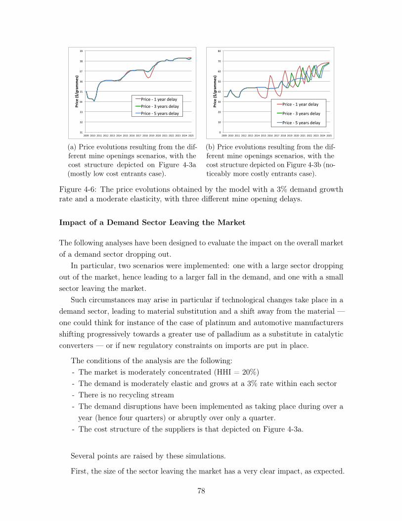
31#

32#

33#

34#

35#

36#

37#

38#

39#

2009# 2010# 2011# 2012# 2013# 2014# 2015# 2016# 2017# 2018# 2019# 2020# 2021# 2022# 2023# 2024# 2025#

Price&($/grammes)&

Price#1#1#year#delay#Price#1#3#years#delay#Price#1#5#years#delay#

(a) Price evolutions resulting from the dif-ferent mine openings scenarios, with thecost structure depicted on Figure 4-3a(mostly low cost entrants case).

0"

10"

20"

30"

40"

50"

60"

70"

80"

2009" 2010" 2011" 2012" 2013" 2014" 2015" 2016" 2017" 2018" 2019" 2020" 2021" 2022" 2023" 2024" 2025"

Price&($/grammes)&

Price"1"1"year"delay"

Price"1"3"years"delay"

Price"1"5"years"delay"

(b) Price evolutions resulting from the dif-ferent mine openings scenarios, with thecost structure depicted on Figure 4-3b (no-ticeably more costly entrants case).

Figure 4-6: The price evolutions obtained by the model with a 3% demand growthrate and a moderate elasticity, with three different mine opening delays.

Impact of a Demand Sector Leaving the Market

The following analyses have been designed to evaluate the impact on the overall marketof a demand sector dropping out.

In particular, two scenarios were implemented: one with a large sector droppingout of the market, hence leading to a larger fall in the demand, and one with a smallsector leaving the market.

Such circumstances may arise in particular if technological changes take place in ademand sector, leading to material substitution and a shift away from the material —one could think for instance of the case of platinum and automotive manufacturersshifting progressively towards a greater use of palladium as a substitute in catalyticconverters — or if new regulatory constraints on imports are put in place.

The conditions of the analysis are the following:- The market is moderately concentrated (HHI = 20%)- The demand is moderately elastic and grows at a 3% rate within each sector- There is no recycling stream- The demand disruptions have been implemented as taking place during over a

year (hence four quarters) or abruptly over only a quarter.- The cost structure of the suppliers is that depicted on Figure 4-3a.

Several points are raised by these simulations.

First, the size of the sector leaving the market has a very clear impact, as expected.

78

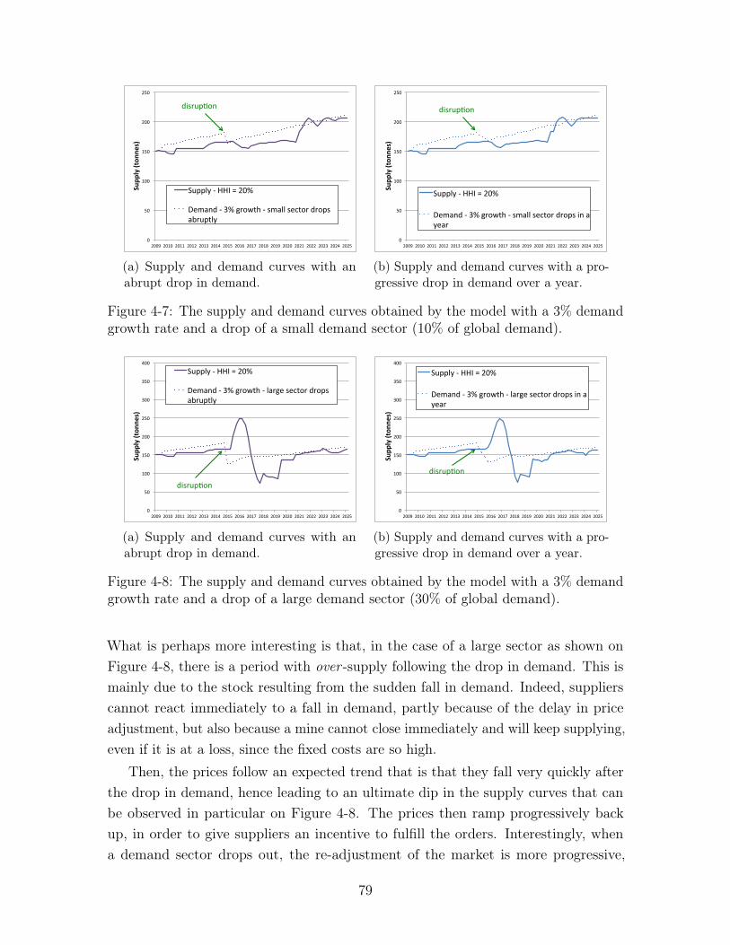
0"

50"

100"

150"

200"

250"

2009" 2010" 2011" 2012" 2013" 2014" 2015" 2016" 2017" 2018" 2019" 2020" 2021" 2022" 2023" 2024" 2025"

Supp

ly&(ton

nes)&

Supply"1"HHI"="20%"

Demand"1"3%"growth"1"small"sector"drops"abruptly"

disrupFon"

(a) Supply and demand curves with anabrupt drop in demand.

0"

50"

100"

150"

200"

250"

2009" 2010" 2011" 2012" 2013" 2014" 2015" 2016" 2017" 2018" 2019" 2020" 2021" 2022" 2023" 2024" 2025"

Supp

ly&(ton

nes)&

Supply"1"HHI"="20%"

Demand"1"3%"growth"1"small"sector"drops"in"a"year"

disrupEon"

(b) Supply and demand curves with a pro-gressive drop in demand over a year.

Figure 4-7: The supply and demand curves obtained by the model with a 3% demandgrowth rate and a drop of a small demand sector (10% of global demand).

0"

50"

100"

150"

200"

250"

300"

350"

400"

2009" 2010" 2011" 2012" 2013" 2014" 2015" 2016" 2017" 2018" 2019" 2020" 2021" 2022" 2023" 2024" 2025"

Supp

ly&(ton

nes)&

Supply"1"HHI"="20%"

Demand"1"3%"growth"1"large"sector"drops"abruptly"

disrupFon"

(a) Supply and demand curves with anabrupt drop in demand.

0"

50"

100"

150"

200"

250"

300"

350"

400"

2009" 2010" 2011" 2012" 2013" 2014" 2015" 2016" 2017" 2018" 2019" 2020" 2021" 2022" 2023" 2024" 2025"

Supp

ly&(ton

nes)&

Supply"1"HHI"="20%"

Demand"1"3%"growth"1"large"sector"drops"in"a"year"

disrupEon"

(b) Supply and demand curves with a pro-gressive drop in demand over a year.

Figure 4-8: The supply and demand curves obtained by the model with a 3% demandgrowth rate and a drop of a large demand sector (30% of global demand).

What is perhaps more interesting is that, in the case of a large sector as shown onFigure 4-8, there is a period with over -supply following the drop in demand. This ismainly due to the stock resulting from the sudden fall in demand. Indeed, supplierscannot react immediately to a fall in demand, partly because of the delay in priceadjustment, but also because a mine cannot close immediately and will keep supplying,even if it is at a loss, since the fixed costs are so high.

Then, the prices follow an expected trend that is that they fall very quickly afterthe drop in demand, hence leading to an ultimate dip in the supply curves that canbe observed in particular on Figure 4-8. The prices then ramp progressively backup, in order to give suppliers an incentive to fulfill the orders. Interestingly, whena demand sector drops out, the re-adjustment of the market is more progressive,

79

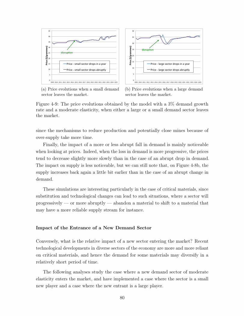
0"

5"

10"

15"

20"

25"

30"

35"

40"

45"

2009" 2010" 2011" 2012" 2013" 2014" 2015" 2016" 2017" 2018" 2019" 2020" 2021" 2022" 2023" 2024" 2025"

Price&($/grammes)&

Price"1"small"sector"drops"in"a"year"

Price"1"small"sector"drops"abruptly"

disrup>on"

(a) Price evolutions when a small demandsector leaves the market.

0"

5"

10"

15"

20"

25"

30"

35"

40"

2009" 2010" 2011" 2012" 2013" 2014" 2015" 2016" 2017" 2018" 2019" 2020" 2021" 2022" 2023" 2024" 2025"

Price&($/grammes)&

Price"1"large"sector"drops"in"a"year"

Price"1"large"sector"drops"abruptly"

disrup>on"

(b) Price evolutions when a large demandsector leaves the market.

Figure 4-9: The price evolutions obtained by the model with a 3% demand growthrate and a moderate elasticity, when either a large or a small demand sector leavesthe market.

since the mechanisms to reduce production and potentially close mines because ofover-supply take more time.

Finally, the impact of a more or less abrupt fall in demand is mainly noticeablewhen looking at prices. Indeed, when the loss in demand is more progressive, the pricestend to decrease slightly more slowly than in the case of an abrupt drop in demand.The impact on supply is less noticeable, but we can still note that, on Figure 4-8b, thesupply increases back again a little bit earlier than in the case of an abrupt change indemand.

These simulations are interesting particularly in the case of critical materials, sincesubstitution and technological changes can lead to such situations, where a sector willprogressively — or more abruptly — abandon a material to shift to a material thatmay have a more reliable supply stream for instance.

Impact of the Entrance of a New Demand Sector

Conversely, what is the relative impact of a new sector entering the market? Recenttechnological developments in diverse sectors of the economy are more and more relianton critical materials, and hence the demand for some materials may diversify in arelatively short period of time.

The following analyses study the case where a new demand sector of moderateelasticity enters the market, and have implemented a case where the sector is a smallnew player and a case where the new entrant is a large player.

80

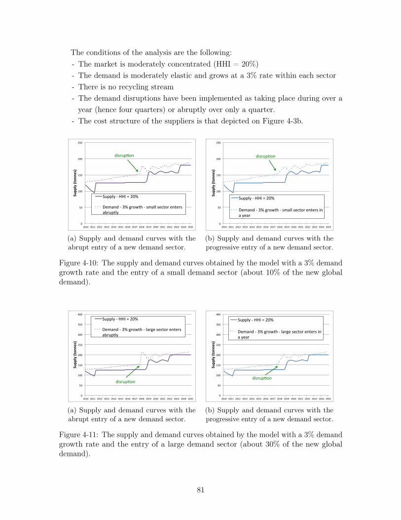
The conditions of the analysis are the following:- The market is moderately concentrated (HHI = 20%)- The demand is moderately elastic and grows at a 3% rate within each sector- There is no recycling stream- The demand disruptions have been implemented as taking place during over a

year (hence four quarters) or abruptly over only a quarter.- The cost structure of the suppliers is that depicted on Figure 4-3b.

0"

50"

100"

150"

200"

250"

2010" 2011" 2012" 2013" 2014" 2015" 2016" 2017" 2018" 2019" 2020" 2021" 2022" 2023" 2024" 2025"

Supp

ly&(ton

nes)&

Supply"1"HHI"="20%"

Demand"1"3%"growth"1"small"sector"enters"abruptly"

disrupFon"

(a) Supply and demand curves with theabrupt entry of a new demand sector.

0"

50"

100"

150"

200"

250"

2010" 2011" 2012" 2013" 2014" 2015" 2016" 2017" 2018" 2019" 2020" 2021" 2022" 2023" 2024" 2025"

Supp

ly&(ton

nes)&

Supply"1"HHI"="20%"

Demand"1"3%"growth"1"small"sector"enters"in"a"year"

disrupEon"

(b) Supply and demand curves with theprogressive entry of a new demand sector.

Figure 4-10: The supply and demand curves obtained by the model with a 3% demandgrowth rate and the entry of a small demand sector (about 10% of the new globaldemand).

0"

50"

100"

150"

200"

250"

300"

350"

400"

2010" 2011" 2012" 2013" 2014" 2015" 2016" 2017" 2018" 2019" 2020" 2021" 2022" 2023" 2024" 2025"

Supp

ly&(ton

nes)&

Supply"1"HHI"="20%"

Demand"1"3%"growth"1"large"sector"enters"abruptly"

disrupFon"

(a) Supply and demand curves with theabrupt entry of a new demand sector.

0"

50"

100"

150"

200"

250"

300"

350"

400"

2010" 2011" 2012" 2013" 2014" 2015" 2016" 2017" 2018" 2019" 2020" 2021" 2022" 2023" 2024" 2025"

Supp

ly&(ton

nes)&

Supply"1"HHI"="20%"

Demand"1"3%"growth"1"large"sector"enters"in"a"year"

disrupEon"

(b) Supply and demand curves with theprogressive entry of a new demand sector.

Figure 4-11: The supply and demand curves obtained by the model with a 3% demandgrowth rate and the entry of a large demand sector (about 30% of the new globaldemand).

81

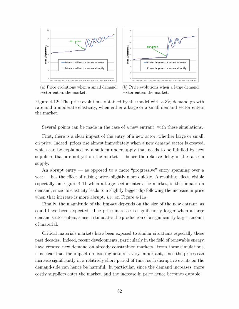
0"

10"

20"

30"

40"

50"

60"

2010" 2011" 2012" 2013" 2014" 2015" 2016" 2017" 2018" 2019" 2020" 2021" 2022" 2023" 2024" 2025"

Price&($/grammes)&

Price"1"small"sector"enters"in"a"year"

Price"1"small"sector"enters"abruptly"

disrup>on"

(a) Price evolutions when a small demandsector enters the market.

0"

10"

20"

30"

40"

50"

60"

70"

80"

2010" 2011" 2012" 2013" 2014" 2015" 2016" 2017" 2018" 2019" 2020" 2021" 2022" 2023" 2024" 2025"

Price&($/grammes)&

Price"1"large"sector"enters"in"a"year"

Price"1"large"sector"enters"abruptly"

disrup>on"

(b) Price evolutions when a large demandsector enters the market.

Figure 4-12: The price evolutions obtained by the model with a 3% demand growthrate and a moderate elasticity, when either a large or a small demand sector entersthe market.

Several points can be made in the case of a new entrant, with these simulations.

First, there is a clear impact of the entry of a new actor, whether large or small,on price. Indeed, prices rise almost immediately when a new demand sector is created,which can be explained by a sudden undersupply that needs to be fulfilled by newsuppliers that are not yet on the market — hence the relative delay in the raise insupply.

An abrupt entry — as opposed to a more “progressive” entry spanning over ayear — has the effect of raising prices slightly more quickly. A resulting effect, visibleespecially on Figure 4-11 when a large sector enters the market, is the impact ondemand, since its elasticity leads to a slightly bigger dip following the increase in pricewhen that increase is more abrupt, i.e. on Figure 4-11a.

Finally, the magnitude of the impact depends on the size of the new entrant, ascould have been expected. The price increase is significantly larger when a largedemand sector enters, since it stimulates the production of a significantly larger amountof material.

Critical materials markets have been exposed to similar situations especially thesepast decades. Indeed, recent developments, particularly in the field of renewable energy,have created new demand on already constrained markets. From these simulations,it is clear that the impact on existing actors is very important, since the prices canincrease significantly in a relatively short period of time; such disruptive events on thedemand-side can hence be harmful. In particular, since the demand increases, morecostly suppliers enter the market, and the increase in price hence becomes durable.

82

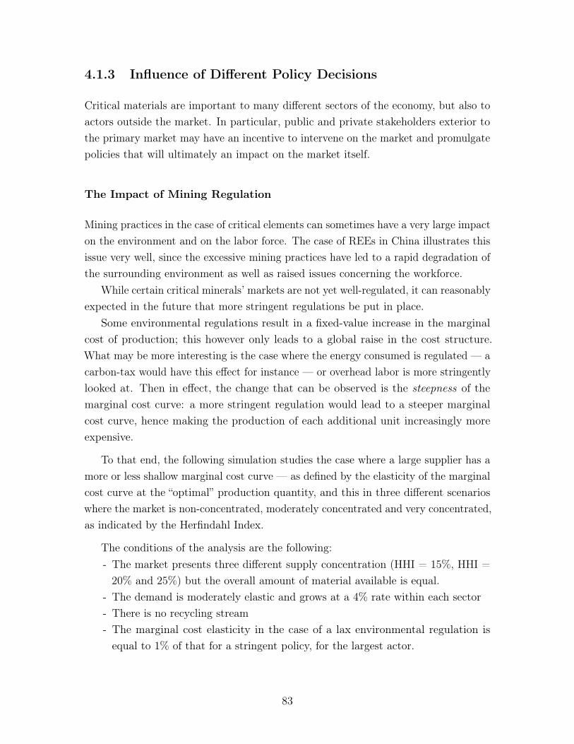
4.1.3 Influence of Different Policy Decisions

Critical materials are important to many different sectors of the economy, but also toactors outside the market. In particular, public and private stakeholders exterior tothe primary market may have an incentive to intervene on the market and promulgatepolicies that will ultimately an impact on the market itself.

The Impact of Mining Regulation

Mining practices in the case of critical elements can sometimes have a very large impacton the environment and on the labor force. The case of REEs in China illustrates thisissue very well, since the excessive mining practices have led to a rapid degradation ofthe surrounding environment as well as raised issues concerning the workforce.

While certain critical minerals’ markets are not yet well-regulated, it can reasonablyexpected in the future that more stringent regulations be put in place.

Some environmental regulations result in a fixed-value increase in the marginalcost of production; this however only leads to a global raise in the cost structure.What may be more interesting is the case where the energy consumed is regulated — acarbon-tax would have this effect for instance — or overhead labor is more stringentlylooked at. Then in effect, the change that can be observed is the steepness of themarginal cost curve: a more stringent regulation would lead to a steeper marginalcost curve, hence making the production of each additional unit increasingly moreexpensive.

To that end, the following simulation studies the case where a large supplier has amore or less shallow marginal cost curve — as defined by the elasticity of the marginalcost curve at the “optimal” production quantity, and this in three different scenarioswhere the market is non-concentrated, moderately concentrated and very concentrated,as indicated by the Herfindahl Index.

The conditions of the analysis are the following:- The market presents three different supply concentration (HHI = 15%, HHI =

20% and 25%) but the overall amount of material available is equal.- The demand is moderately elastic and grows at a 4% rate within each sector- There is no recycling stream- The marginal cost elasticity in the case of a lax environmental regulation is

equal to 1% of that for a stringent policy, for the largest actor.

83

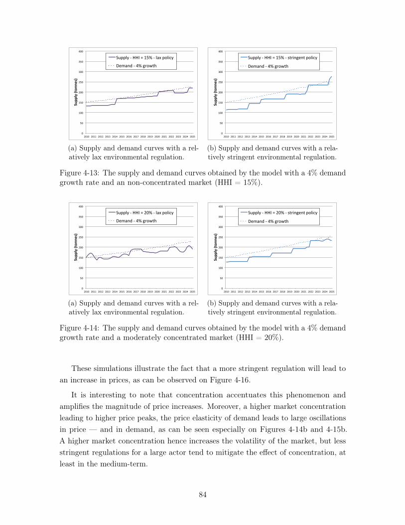
0"

50"

100"

150"

200"

250"

300"

350"

400"

2010" 2011" 2012" 2013" 2014" 2015" 2016" 2017" 2018" 2019" 2020" 2021" 2022" 2023" 2024" 2025"

Supp

ly&(ton

nes)&

Supply"1"HHI"="15%"1"lax"policy"

Demand"1"4%"growth"

(a) Supply and demand curves with a rel-atively lax environmental regulation.

0"

50"

100"

150"

200"

250"

300"

350"

400"

2010" 2011" 2012" 2013" 2014" 2015" 2016" 2017" 2018" 2019" 2020" 2021" 2022" 2023" 2024" 2025"

Supp

ly&(ton

nes)&

Supply"1"HHI"="15%"1"stringent"policy"

Demand"1"4%"growth"

(b) Supply and demand curves with a rela-tively stringent environmental regulation.

Figure 4-13: The supply and demand curves obtained by the model with a 4% demandgrowth rate and an non-concentrated market (HHI = 15%).

0"

50"

100"

150"

200"

250"

300"

350"

400"

2010" 2011" 2012" 2013" 2014" 2015" 2016" 2017" 2018" 2019" 2020" 2021" 2022" 2023" 2024" 2025"

Supp

ly&(ton

nes)&

Supply"1"HHI"="20%"1"lax"policy"

Demand"1"4%"growth"

(a) Supply and demand curves with a rel-atively lax environmental regulation.

0"

50"

100"

150"

200"

250"

300"

350"

400"

2010" 2011" 2012" 2013" 2014" 2015" 2016" 2017" 2018" 2019" 2020" 2021" 2022" 2023" 2024" 2025"

Supp

ly&(ton

nes)&

Supply"1"HHI"="20%"1"stringent"policy"

Demand"1"4%"growth"

(b) Supply and demand curves with a rela-tively stringent environmental regulation.

Figure 4-14: The supply and demand curves obtained by the model with a 4% demandgrowth rate and a moderately concentrated market (HHI = 20%).

These simulations illustrate the fact that a more stringent regulation will lead toan increase in prices, as can be observed on Figure 4-16.

It is interesting to note that concentration accentuates this phenomenon andamplifies the magnitude of price increases. Moreover, a higher market concentrationleading to higher price peaks, the price elasticity of demand leads to large oscillationsin price — and in demand, as can be seen especially on Figures 4-14b and 4-15b.A higher market concentration hence increases the volatility of the market, but lessstringent regulations for a large actor tend to mitigate the effect of concentration, atleast in the medium-term.

84

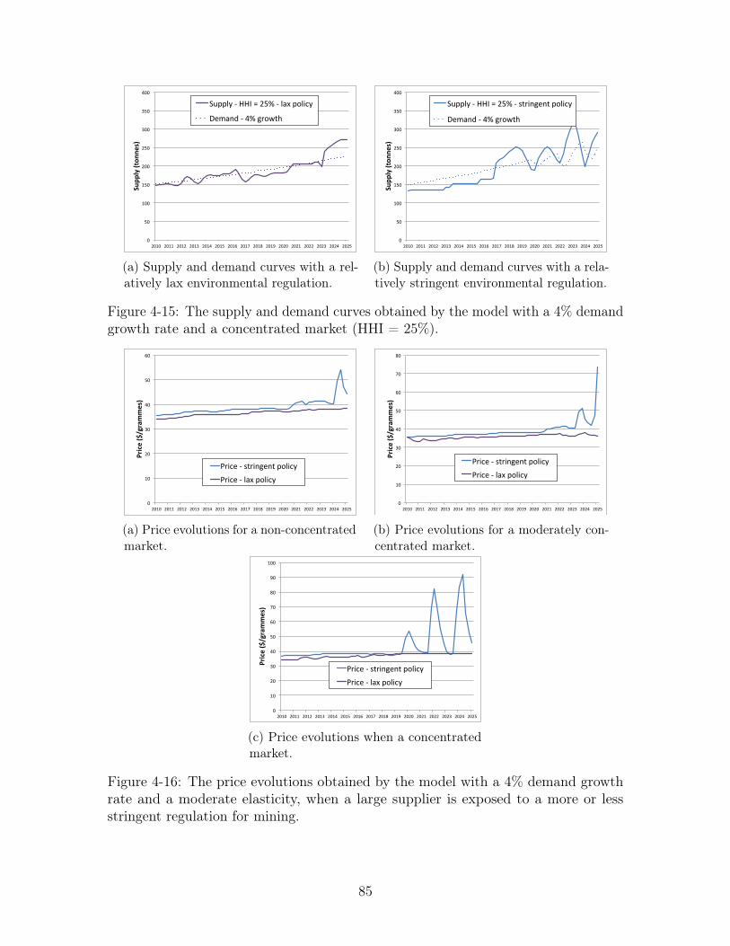
0"

50"

100"

150"

200"

250"

300"

350"

400"

2010" 2011" 2012" 2013" 2014" 2015" 2016" 2017" 2018" 2019" 2020" 2021" 2022" 2023" 2024" 2025"

Supp

ly&(ton

nes)&

Supply"1"HHI"="25%"1"lax"policy"

Demand"1"4%"growth"

(a) Supply and demand curves with a rel-atively lax environmental regulation.

0"

50"

100"

150"

200"

250"

300"

350"

400"

2010" 2011" 2012" 2013" 2014" 2015" 2016" 2017" 2018" 2019" 2020" 2021" 2022" 2023" 2024" 2025"

Supp

ly&(ton

nes)&

Supply"1"HHI"="25%"1"stringent"policy"

Demand"1"4%"growth"

(b) Supply and demand curves with a rela-tively stringent environmental regulation.

Figure 4-15: The supply and demand curves obtained by the model with a 4% demandgrowth rate and a concentrated market (HHI = 25%).

0"

10"

20"

30"

40"

50"

60"

2010" 2011" 2012" 2013" 2014" 2015" 2016" 2017" 2018" 2019" 2020" 2021" 2022" 2023" 2024" 2025"

Price&($/grammes)&

Price"1"stringent"policy"Price"1"lax"policy"

(a) Price evolutions for a non-concentratedmarket.

0"

10"

20"

30"

40"

50"

60"

70"

80"

2010" 2011" 2012" 2013" 2014" 2015" 2016" 2017" 2018" 2019" 2020" 2021" 2022" 2023" 2024" 2025"

Price&($/grammes)&

Price"1"stringent"policy"Price"1"lax"policy"

(b) Price evolutions for a moderately con-centrated market.

0"

10"

20"

30"

40"

50"

60"

70"

80"

90"

100"

2010" 2011" 2012" 2013" 2014" 2015" 2016" 2017" 2018" 2019" 2020" 2021" 2022" 2023" 2024" 2025"

Price&($/grammes)&

Price"1"stringent"policy"Price"1"lax"policy"

(c) Price evolutions when a concentratedmarket.

Figure 4-16: The price evolutions obtained by the model with a 4% demand growthrate and a moderate elasticity, when a large supplier is exposed to a more or lessstringent regulation for mining.

85

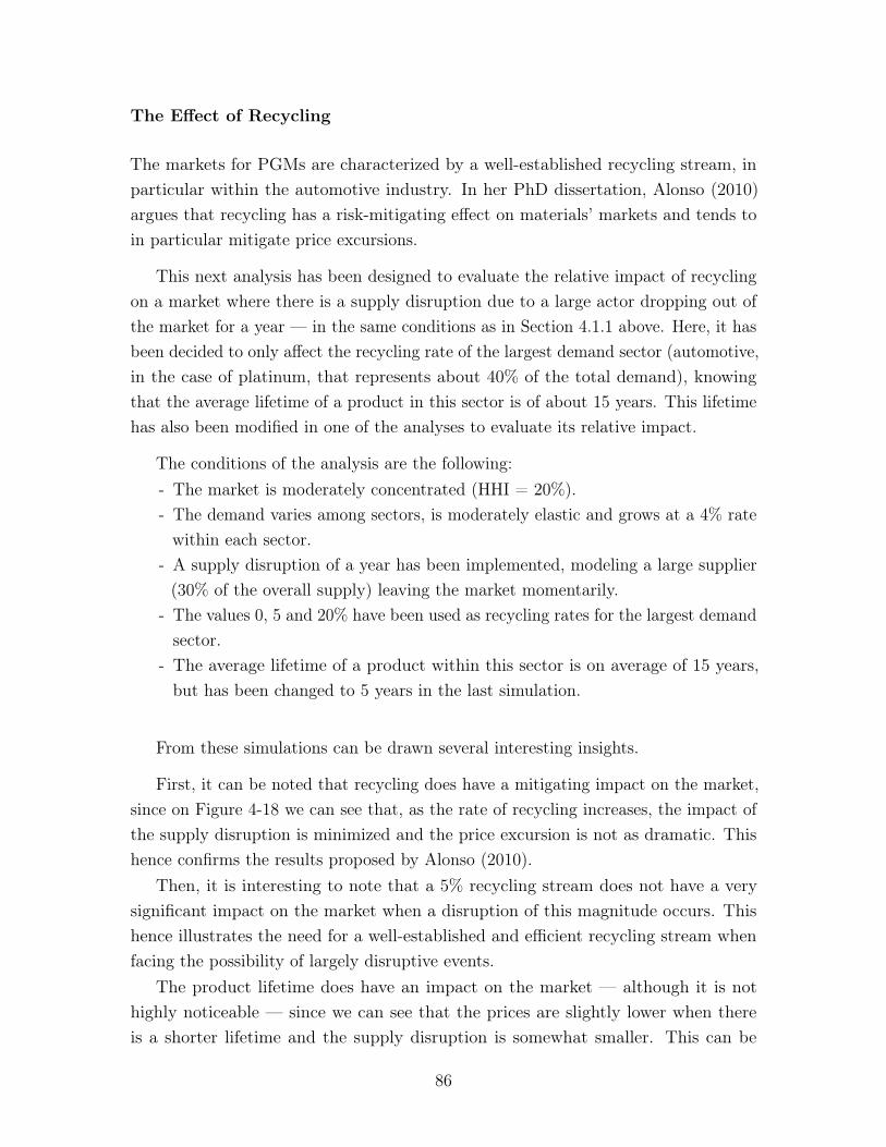
The Effect of Recycling

The markets for PGMs are characterized by a well-established recycling stream, inparticular within the automotive industry. In her PhD dissertation, Alonso (2010)argues that recycling has a risk-mitigating effect on materials’ markets and tends toin particular mitigate price excursions.

This next analysis has been designed to evaluate the relative impact of recyclingon a market where there is a supply disruption due to a large actor dropping out ofthe market for a year — in the same conditions as in Section 4.1.1 above. Here, it hasbeen decided to only affect the recycling rate of the largest demand sector (automotive,in the case of platinum, that represents about 40% of the total demand), knowingthat the average lifetime of a product in this sector is of about 15 years. This lifetimehas also been modified in one of the analyses to evaluate its relative impact.

The conditions of the analysis are the following:- The market is moderately concentrated (HHI = 20%).- The demand varies among sectors, is moderately elastic and grows at a 4% rate

within each sector.- A supply disruption of a year has been implemented, modeling a large supplier

(30% of the overall supply) leaving the market momentarily.- The values 0, 5 and 20% have been used as recycling rates for the largest demand

sector.- The average lifetime of a product within this sector is on average of 15 years,

but has been changed to 5 years in the last simulation.

From these simulations can be drawn several interesting insights.

First, it can be noted that recycling does have a mitigating impact on the market,since on Figure 4-18 we can see that, as the rate of recycling increases, the impact ofthe supply disruption is minimized and the price excursion is not as dramatic. Thishence confirms the results proposed by Alonso (2010).

Then, it is interesting to note that a 5% recycling stream does not have a verysignificant impact on the market when a disruption of this magnitude occurs. Thishence illustrates the need for a well-established and efficient recycling stream whenfacing the possibility of largely disruptive events.

The product lifetime does have an impact on the market — although it is nothighly noticeable — since we can see that the prices are slightly lower when thereis a shorter lifetime and the supply disruption is somewhat smaller. This can be

86

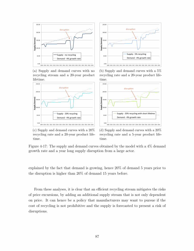
0.00#

50.00#

100.00#

150.00#

200.00#

250.00#

2009# 2010# 2011# 2012# 2013# 2014# 2015# 2016# 2017# 2018# 2019# 2020# 2021# 2022# 2023# 2024# 2025#

Supp

ly&(ton

nes)&

Supply#2#no#recycling#

Demand#2#4%#growth#rate#

disrupCon#

(a) Supply and demand curves with norecycling stream and a 20-year productlifetime.

0.00#

50.00#

100.00#

150.00#

200.00#

250.00#

2009# 2010# 2011# 2012# 2013# 2014# 2015# 2016# 2017# 2018# 2019# 2020# 2021# 2022# 2023# 2024# 2025#

Supp

ly&(ton

nes)&

Supply#2#5%#recycling#

Demand#2#4%#growth#rate#

disrupCon#

(b) Supply and demand curves with a 5%recycling rate and a 20-year product life-time.

0.00#

50.00#

100.00#

150.00#

200.00#

250.00#

2009# 2010# 2011# 2012# 2013# 2014# 2015# 2016# 2017# 2018# 2019# 2020# 2021# 2022# 2023# 2024# 2025#

Supp

ly&(ton

nes)&

Supply#2#20%#recycling#

Demand#2#4%#growth#rate#

disrupCon#

(c) Supply and demand curves with a 20%recycling rate and a 20-year product life-time.

0.00#

50.00#

100.00#

150.00#

200.00#

250.00#

2009# 2010# 2011# 2012# 2013# 2014# 2015# 2016# 2017# 2018# 2019# 2020# 2021# 2022# 2023# 2024# 2025#

Supp

ly&(ton

nes)&

Supply#2#20%#recycling#with#short#life@me#

Demand#2#4%#growth#rate#

disrup@on#

(d) Supply and demand curves with a 20%recycling rate and a 5-year product life-time.

Figure 4-17: The supply and demand curves obtained by the model with a 4% demandgrowth rate and a year long supply disruption from a large actor.

explained by the fact that demand is growing, hence 20% of demand 5 years prior tothe disruption is higher than 20% of demand 15 years before.

From these analyses, it is clear that an efficient recycling stream mitigates the risksof price excursions, by adding an additional supply stream that is not only dependenton price. It can hence be a policy that manufacturers may want to pursue if thecost of recycling is not prohibitive and the supply is forecasted to present a risk ofdisruptions.

87

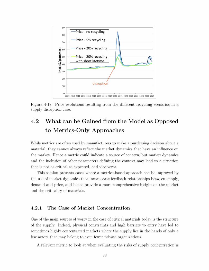
0"

10"

20"

30"

40"

50"

60"

70"

80"

90"

2009" 2010" 2011" 2012" 2013" 2014" 2015" 2016" 2017" 2018" 2019" 2020" 2021" 2022" 2023" 2024" 2025"

Price&($/grammes)&

Price"1"no"recycling"

Price"1"5%"recycling"

Price"1"20%"recycling"

Price"1"20%"recycling"with"short"life=me"

disrup=on"

Figure 4-18: Price evolutions resulting from the different recycling scenarios in asupply disruption case.

4.2 What can be Gained from the Model as Opposedto Metrics-Only Approaches

While metrics are often used by manufacturers to make a purchasing decision about amaterial, they cannot always reflect the market dynamics that have an influence onthe market. Hence a metric could indicate a source of concern, but market dynamicsand the inclusion of other parameters defining the context may lead to a situationthat is not as critical as expected, and vice versa.

This section presents cases where a metrics-based approach can be improved bythe use of market dynamics that incorporate feedback relationships between supply,demand and price, and hence provide a more comprehensive insight on the marketand the criticality of materials.

4.2.1 The Case of Market Concentration

One of the main sources of worry in the case of critical materials today is the structureof the supply. Indeed, physical constraints and high barriers to entry have led tosometimes highly concentrated markets where the supply lies in the hands of only afew actors that may belong to even fewer private organizations.

A relevant metric to look at when evaluating the risks of supply concentration is

88

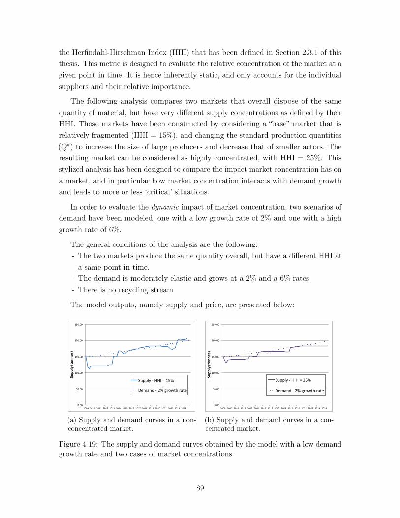
the Herfindahl-Hirschman Index (HHI) that has been defined in Section 2.3.1 of thisthesis. This metric is designed to evaluate the relative concentration of the market at agiven point in time. It is hence inherently static, and only accounts for the individualsuppliers and their relative importance.

The following analysis compares two markets that overall dispose of the samequantity of material, but have very different supply concentrations as defined by theirHHI. Those markets have been constructed by considering a “base” market that isrelatively fragmented (HHI = 15%), and changing the standard production quantities(Q⇤) to increase the size of large producers and decrease that of smaller actors. Theresulting market can be considered as highly concentrated, with HHI = 25%. Thisstylized analysis has been designed to compare the impact market concentration has ona market, and in particular how market concentration interacts with demand growthand leads to more or less ‘critical’ situations.

In order to evaluate the dynamic impact of market concentration, two scenarios ofdemand have been modeled, one with a low growth rate of 2% and one with a highgrowth rate of 6%.

The general conditions of the analysis are the following:- The two markets produce the same quantity overall, but have a different HHI at

a same point in time.- The demand is moderately elastic and grows at a 2% and a 6% rates- There is no recycling stream

The model outputs, namely supply and price, are presented below:

0.00#

50.00#

100.00#

150.00#

200.00#

250.00#

2009# 2010# 2011# 2012# 2013# 2014# 2015# 2016# 2017# 2018# 2019# 2020# 2021# 2022# 2023# 2024#

Supp

ly&(ton

nes)&

Supply#2#HHI#=#15%#

Demand#2#2%#growth#rate#

(a) Supply and demand curves in a non-concentrated market.

0.00#

50.00#

100.00#

150.00#

200.00#

250.00#

2009# 2010# 2011# 2012# 2013# 2014# 2015# 2016# 2017# 2018# 2019# 2020# 2021# 2022# 2023# 2024#

Supp

ly&(ton

nes)&

Supply#2#HHI#=#25%#

Demand#2#2%#growth#rate#

(b) Supply and demand curves in a con-centrated market.

Figure 4-19: The supply and demand curves obtained by the model with a low demandgrowth rate and two cases of market concentrations.

89

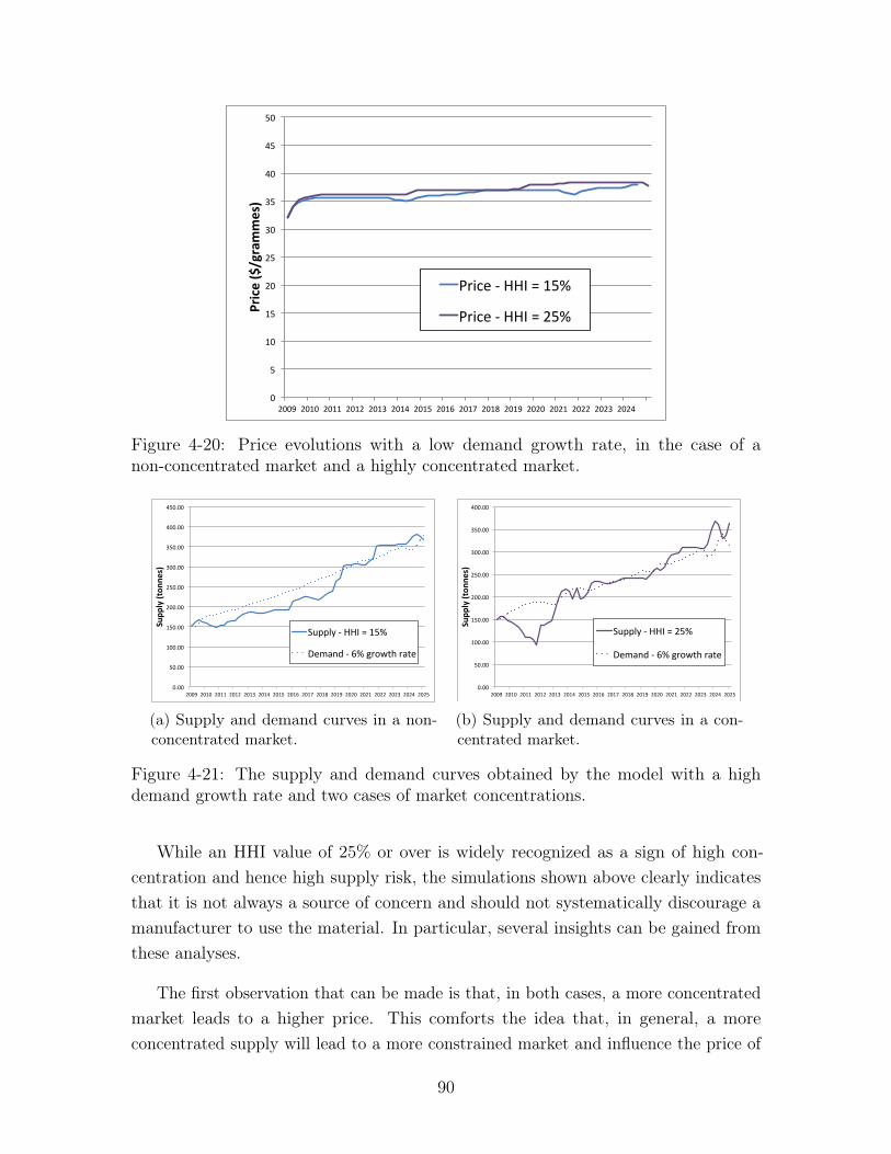
0"

5"

10"

15"

20"

25"

30"

35"

40"

45"

50"

2009" 2010" 2011" 2012" 2013" 2014" 2015" 2016" 2017" 2018" 2019" 2020" 2021" 2022" 2023" 2024"

Price&($/grammes)&

Price"1"HHI"="15%"

Price"1"HHI"="25%"

Figure 4-20: Price evolutions with a low demand growth rate, in the case of anon-concentrated market and a highly concentrated market.

0.00#

50.00#

100.00#

150.00#

200.00#

250.00#

300.00#

350.00#

400.00#

450.00#

2009# 2010# 2011# 2012# 2013# 2014# 2015# 2016# 2017# 2018# 2019# 2020# 2021# 2022# 2023# 2024# 2025#

Supp

ly&(ton

nes)&

Supply#2#HHI#=#15%#

Demand#2#6%#growth#rate#

(a) Supply and demand curves in a non-concentrated market.

0.00#

50.00#

100.00#

150.00#

200.00#

250.00#

300.00#

350.00#

400.00#

2009# 2010# 2011# 2012# 2013# 2014# 2015# 2016# 2017# 2018# 2019# 2020# 2021# 2022# 2023# 2024# 2025#

Supp

ly&(ton

nes)&

Supply#2#HHI#=#25%#

Demand#2#6%#growth#rate#

(b) Supply and demand curves in a con-centrated market.

Figure 4-21: The supply and demand curves obtained by the model with a highdemand growth rate and two cases of market concentrations.

While an HHI value of 25% or over is widely recognized as a sign of high con-centration and hence high supply risk, the simulations shown above clearly indicatesthat it is not always a source of concern and should not systematically discourage amanufacturer to use the material. In particular, several insights can be gained fromthese analyses.

The first observation that can be made is that, in both cases, a more concentratedmarket leads to a higher price. This comforts the idea that, in general, a moreconcentrated supply will lead to a more constrained market and influence the price of

90

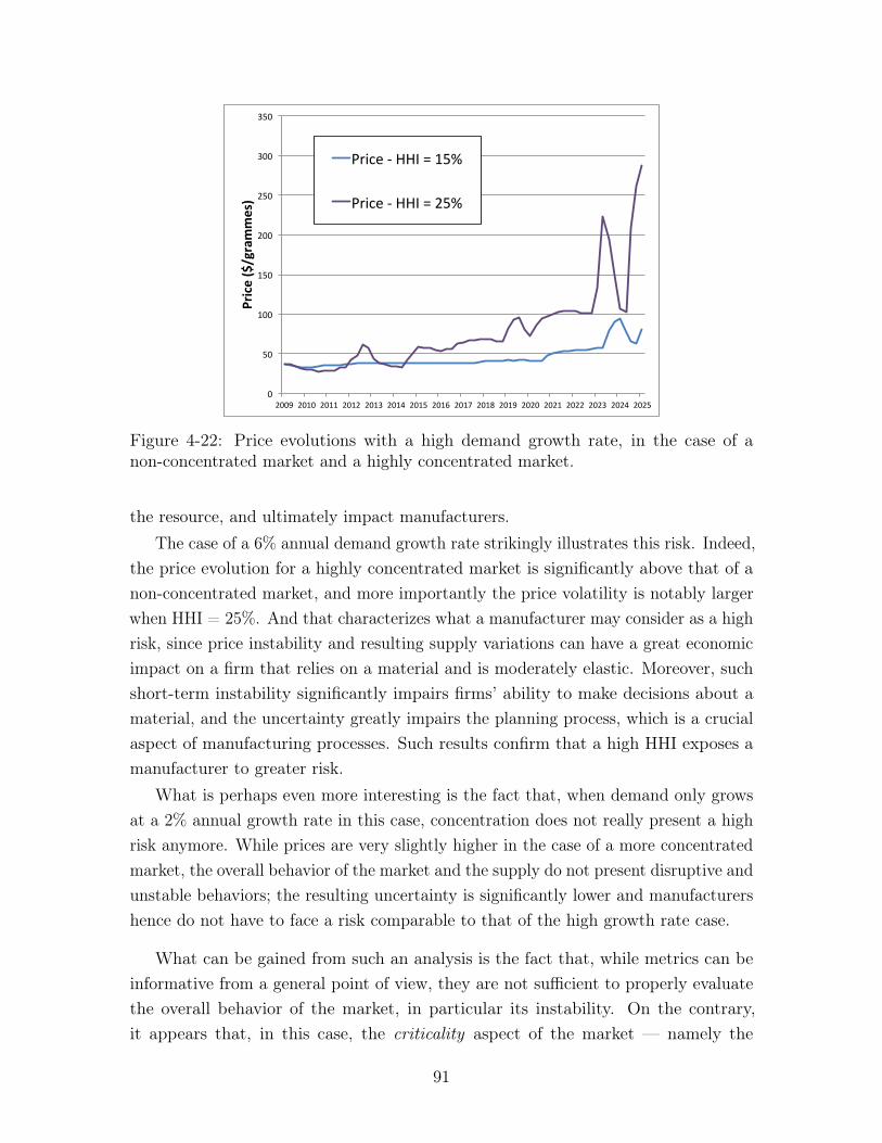
0"

50"

100"

150"

200"

250"

300"

350"

2009" 2010" 2011" 2012" 2013" 2014" 2015" 2016" 2017" 2018" 2019" 2020" 2021" 2022" 2023" 2024" 2025"

Price&($/grammes)&

Price"1"HHI"="15%"

Price"1"HHI"="25%"

Figure 4-22: Price evolutions with a high demand growth rate, in the case of anon-concentrated market and a highly concentrated market.

the resource, and ultimately impact manufacturers.The case of a 6% annual demand growth rate strikingly illustrates this risk. Indeed,

the price evolution for a highly concentrated market is significantly above that of anon-concentrated market, and more importantly the price volatility is notably largerwhen HHI = 25%. And that characterizes what a manufacturer may consider as a highrisk, since price instability and resulting supply variations can have a great economicimpact on a firm that relies on a material and is moderately elastic. Moreover, suchshort-term instability significantly impairs firms’ ability to make decisions about amaterial, and the uncertainty greatly impairs the planning process, which is a crucialaspect of manufacturing processes. Such results confirm that a high HHI exposes amanufacturer to greater risk.

What is perhaps even more interesting is the fact that, when demand only growsat a 2% annual growth rate in this case, concentration does not really present a highrisk anymore. While prices are very slightly higher in the case of a more concentratedmarket, the overall behavior of the market and the supply do not present disruptive andunstable behaviors; the resulting uncertainty is significantly lower and manufacturershence do not have to face a risk comparable to that of the high growth rate case.

What can be gained from such an analysis is the fact that, while metrics can beinformative from a general point of view, they are not sufficient to properly evaluatethe overall behavior of the market, in particular its instability. On the contrary,it appears that, in this case, the criticality aspect of the market — namely the

91

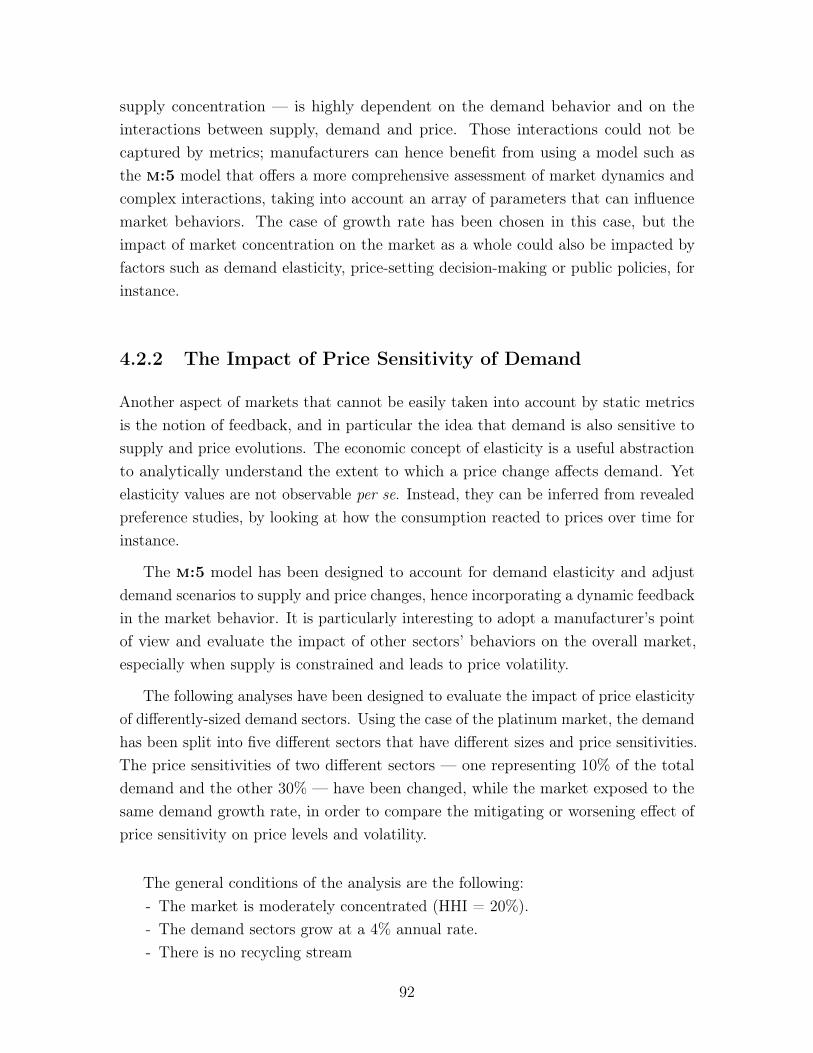
supply concentration — is highly dependent on the demand behavior and on theinteractions between supply, demand and price. Those interactions could not becaptured by metrics; manufacturers can hence benefit from using a model such asthe m:5 model that offers a more comprehensive assessment of market dynamics andcomplex interactions, taking into account an array of parameters that can influencemarket behaviors. The case of growth rate has been chosen in this case, but theimpact of market concentration on the market as a whole could also be impacted byfactors such as demand elasticity, price-setting decision-making or public policies, forinstance.

4.2.2 The Impact of Price Sensitivity of Demand

Another aspect of markets that cannot be easily taken into account by static metricsis the notion of feedback, and in particular the idea that demand is also sensitive tosupply and price evolutions. The economic concept of elasticity is a useful abstractionto analytically understand the extent to which a price change affects demand. Yetelasticity values are not observable per se. Instead, they can be inferred from revealedpreference studies, by looking at how the consumption reacted to prices over time forinstance.

The m:5 model has been designed to account for demand elasticity and adjustdemand scenarios to supply and price changes, hence incorporating a dynamic feedbackin the market behavior. It is particularly interesting to adopt a manufacturer’s pointof view and evaluate the impact of other sectors’ behaviors on the overall market,especially when supply is constrained and leads to price volatility.

The following analyses have been designed to evaluate the impact of price elasticityof differently-sized demand sectors. Using the case of the platinum market, the demandhas been split into five different sectors that have different sizes and price sensitivities.The price sensitivities of two different sectors — one representing 10% of the totaldemand and the other 30% — have been changed, while the market exposed to thesame demand growth rate, in order to compare the mitigating or worsening effect ofprice sensitivity on price levels and volatility.

The general conditions of the analysis are the following:- The market is moderately concentrated (HHI = 20%).- The demand sectors grow at a 4% annual rate.- There is no recycling stream

92

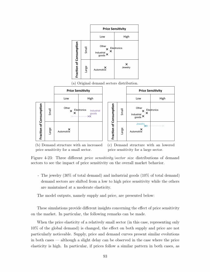
Price&Sensi*vity&

Low$ High$

Frac*o

n&of&Con

sump*

on&

Small$

Large$

Industrial goods

Other Electronics

Jewelry Automotive

(a) Original demand sectors distribution.

Price&Sensi*vity&

Low$ High$

Frac*o

n&of&Con

sump*

on&

Small$

Large$

Industrial goods

Other Electronics

Automotive

(b) Demand structure with an increasedprice sensitivity for a small sector.

Price&Sensi*vity&

Low$ High$

Frac*o

n&of&Con

sump*

on&

Small$

Large$

Industrial goods

Other Electronics

Jewelry

Automotive

(c) Demand structure with an loweredprice sensitivity for a large sector.

Figure 4-23: Three different price sensitivity/sector size distributions of demandsectors to see the impact of price sensitivity on the overall market behavior.

- The jewelry (30% of total demand) and industrial goods (10% of total demand)demand sectors are shifted from a low to high price sensitivity while the othersare maintained at a moderate elasticity.

The model outputs, namely supply and price, are presented below:

These simulations provide different insights concerning the effect of price sensitivityon the market. In particular, the following remarks can be made.

When the price elasticity of a relatively small sector (in this case, representing only10% of the global demand) is changed, the effect on both supply and price are notparticularly noticeable. Supply, price and demand curves present similar evolutionsin both cases — although a slight delay can be observed in the case where the priceelasticity is high. In particular, if prices follow a similar pattern in both cases, as

93

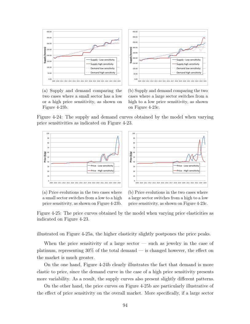
0.00#

50.00#

100.00#

150.00#

200.00#

250.00#

300.00#

350.00#

400.00#

2009# 2010# 2011# 2012# 2013# 2014# 2015# 2016# 2017# 2018# 2019# 2020# 2021# 2022# 2023# 2024# 2025#

Supp

ly&(ton

nes)&

Supply#2#Low#sensi:vity#

Supply#high#sensi:vity#

Demand#low#sensi:vity#

Demand#high#sensi:vity#

(a) Supply and demand comparing thetwo cases where a small sector has a lowor a high price sensitivity, as shown onFigure 4-23b.

0.00#

50.00#

100.00#

150.00#

200.00#

250.00#

300.00#

350.00#

400.00#

450.00#

2009# 2010# 2011# 2012# 2013# 2014# 2015# 2016# 2017# 2018# 2019# 2020# 2021# 2022# 2023# 2024# 2025#

Supp

ly&(ton

nes)&

Supply#2#Low#sensi:vity#

Supply#high#sensi:vity#

Demand#low#sensi:vity#

Demand#high#sensi:vity#

(b) Supply and demand comparing the twocases where a large sector switches from ahigh to a low price sensitivity, as shownon Figure 4-23c.

Figure 4-24: The supply and demand curves obtained by the model when varyingprice sensitivities as indicated on Figure 4-23.

0"

10"

20"

30"

40"

50"

60"

70"

80"

90"

100"

2009" 2010" 2011" 2012" 2013" 2014" 2015" 2016" 2017" 2018" 2019" 2020" 2021" 2022" 2023" 2024" 2025"

Price&($/g)&

Price"1"Low"sensi7vity"

Price"1"High"sensi7vity"

(a) Price evolutions in the two cases wherea small sector switches from a low to a highprice sensitivity, as shown on Figure 4-23b.

0"

10"

20"

30"

40"

50"

60"

70"

80"

90"

100"

2009" 2010" 2011" 2012" 2013" 2014" 2015" 2016" 2017" 2018" 2019" 2020" 2021" 2022" 2023" 2024" 2025"

Price&($/g)&

Price"1"Low"sensi7vity"

Price"1"High"sensi7vity"

(b) Price evolutions in the two cases wherea large sector switches from a high to a lowprice sensitivity, as shown on Figure 4-23c.

Figure 4-25: The price curves obtained by the model when varying price elasticities asindicated on Figure 4-23.

illustrated on Figure 4-25a, the higher elasticity slightly postpones the price peaks.

When the price sensitivity of a large sector — such as jewelry in the case ofplatinum, representing 30% of the total demand — is changed however, the effect onthe market is much greater.

On the one hand, Figure 4-24b clearly illustrates the fact that demand is moreelastic to price, since the demand curve in the case of a high price sensitivity presentsmore variability. As a result, the supply curves also present slightly different patterns.

On the other hand, the price curves on Figure 4-25b are particularly illustrative ofthe effect of price sensitivity on the overall market. More specifically, if a large sector

94

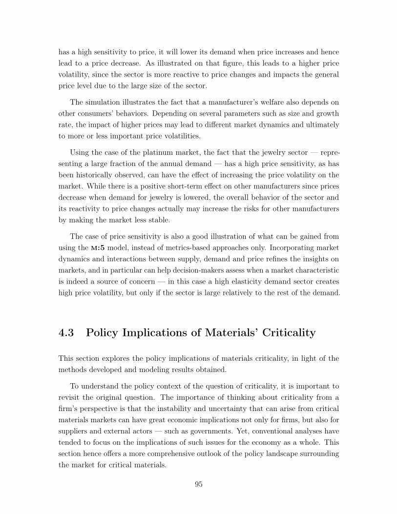
has a high sensitivity to price, it will lower its demand when price increases and hencelead to a price decrease. As illustrated on that figure, this leads to a higher pricevolatility, since the sector is more reactive to price changes and impacts the generalprice level due to the large size of the sector.

The simulation illustrates the fact that a manufacturer’s welfare also depends onother consumers’ behaviors. Depending on several parameters such as size and growthrate, the impact of higher prices may lead to different market dynamics and ultimatelyto more or less important price volatilities.

Using the case of the platinum market, the fact that the jewelry sector — repre-senting a large fraction of the annual demand — has a high price sensitivity, as hasbeen historically observed, can have the effect of increasing the price volatility on themarket. While there is a positive short-term effect on other manufacturers since pricesdecrease when demand for jewelry is lowered, the overall behavior of the sector andits reactivity to price changes actually may increase the risks for other manufacturersby making the market less stable.

The case of price sensitivity is also a good illustration of what can be gained fromusing the m:5 model, instead of metrics-based approaches only. Incorporating marketdynamics and interactions between supply, demand and price refines the insights onmarkets, and in particular can help decision-makers assess when a market characteristicis indeed a source of concern — in this case a high elasticity demand sector createshigh price volatility, but only if the sector is large relatively to the rest of the demand.

4.3 Policy Implications of Materials’ Criticality

This section explores the policy implications of materials criticality, in light of themethods developed and modeling results obtained.

To understand the policy context of the question of criticality, it is important torevisit the original question. The importance of thinking about criticality from afirm’s perspective is that the instability and uncertainty that can arise from criticalmaterials markets can have great economic implications not only for firms, but also forsuppliers and external actors — such as governments. Yet, conventional analyses havetended to focus on the implications of such issues for the economy as a whole. Thissection hence offers a more comprehensive outlook of the policy landscape surroundingthe market for critical materials.

95

The Structure-Conduct-Performance framework applied to critical materials mar-kets in Section 2.1.3, illustrated the concept that markets are influenced not only bytheir primary actors, but are also shaped by external factors such as that of govern-mental policy, and hence have wider policy implications. The following sections usecomponents of this framework to comprehensively suggest and evaluate the differenttypes of policies — whether private or public — that can be implemented, as well astheir possible limitations.

While supply disruptions and price volatility are primary manifestations of what isusually characterized as materials criticality, price volatility information alone does notafford sufficient insight for the task of devising an efficient mitigating policy. Moreover,some of the current rules of thumb for both evaluating and treating materials criticality— such as a focus on market concentration — are potentially too simplistic in bothconception and implementation when the market system as a whole is taken intoconsideration. It then becomes important to establish the circumstances under whichsuch concerns are legitimate in order to avoid unnecessary policy interventions.

The risk-assessment and mitigation process thus has to be decomposed in differentphases, namely to understand (a) whether or not there is a risk, (b) what the magnitudeand the consequences of that risk are, and (c) what types of action can be takenin order to mitigate the effects of the risk, or lower the risk, if possible. The toolsdeveloped in this research have been designed to accomplish those tasks.

A particularly interesting feature of the model is that it aims at understandingwhat the price actually means in the context of critical materials, as well as how thisunderstanding can help guide the decision-maker towards achieving the policy goal ofall market actors: surviving by making the largest profit possible.

Using a decision tool such as the m:5 model is particularly relevant when rec-ognizing that market circumstances continuously evolve and that individual actionshave a broader impact on the market as a whole because of market dynamics andinteractions. Policy-making in the context of critical materials markets should be donein an adaptive way; the use of a model such as the m:5 model, incorporating dynamics,is hence valuable in the pursuit of this goal. An individual decision-maker can usethe model to (a) know what to monitor on the market, and (b) compare the differentpolicies that can be effective or not with the different circumstances surrounding themarket, and this on a regular basis.

Given the constraints arising from the ways in which risks have to be assessed in thecase of critical materials, this section suggests and assesses risk-mitigating strategies

96

that the different market actors — namely suppliers, consumers and policy-makers —can implement, using model insights and reflections on critical materials’ markets.

4.3.1 Policies to Influence the Supply Market Structure

Historical events, reinforced by model simulations, have shown that several structuralcharacteristics of materials’ markets present inefficiencies that ultimately can leadto higher risks of supply disruptions and price excursions: the number of supplierson the market, the barriers to entry, and the cost structure of the different actors.This section aims at giving ways in which market actors may influence the structureof such markets to mitigate the risks associated with the structural inefficiencies ofmaterials’ supply.

Addressing the Issue of “Natural” Market Concentration

One of the most important concerns on the supply-side of materials markets isthe influence of high market concentration on market efficiency. Mining marketsare characterized by very constrained supply structures, arising from (a) physicalconstraints due to the geographic distribution of resources and (b) high investmentand capital requirements. Supply concentration can lead to more substantial priceexcursions during periods of rapid growth in demand, as has been seen in the case ofpalladium presented in Section 2.2 and in the results of model simulation presented inSection 4.2.1 for instance. While concentration cannot systematically be consideredas a structural market characteristic, especially if the monopolistic or oligopolisticpositions of certain suppliers have been acquired through a particular conduct, thissection only considers cases where market concentration arises due to the naturaldistribution of resources.

Policies that can be adopted in the case of a “natural” mono- or oligopoly arelimited however, because of the very nature of the problem.

Private actors, particularly suppliers and consumers, may have an incentive tointervene to mitigate the effects of a “natural” mono- or oligopolistic situation onthe market, rather than try to correct the situation itself. In particular, recyclingappears to be an efficient policy, since adding a secondary supply stream to theprimary production can have a risk-mitigating effect — particularly in the case ofsupply disruption — as observed by Alonso (2010) and shown by model simulations.Interestingly, the amount of material that can be recycled at each period depends

97

on past consumption and not directly on supply nor supply structure — though onecould expect price to influence the rate of recycling, providing a more or less attractiveincentive to develop a sustainable and efficient recycling stream.

For manufacturers, improving recycling can be a beneficial policy for additionalreasons. In particular, increasing the recyclability of material or making the recyclingprocess more efficient has a positive influence on the sustainability aspect of thematerial, which can be interesting in particular if regulations encourage the use ofsecondary material.

An important aspect to consider when implementing a recycling policy is the notionof timeframe. Indeed, materials can only be recycled once the products they wereembedded in reach their lifetime. Such lifetime may be difficult to forecast and henceit becomes difficult for manufacturers to evaluate precisely how large the secondarysupply will be at a given time. Moreover, the efficiency of recovery highly depends onthe products the material was used in, as well as on the process required to recycleand re-condition the material so that it can be used again.

Another important question arising when considering the implementation of a recy-cling stream is that of who should take on the recycling process. While manufacturershave definite advantages to encourage recycling policies in order to stabilize supplyand prices, and potentially improve the material’s sustainability impact, the cost ofrecycling may be prohibitive or the facilities to accomplish a sustainable recyclingstream too capital-intensive. On the other hand, suppliers may have an incentiveto undertake recycling operations as well; if the recovery process is compatible withmining and processing processes, it can be beneficial to increase revenues by providinga secondary supply stream.

Enforcing a more efficient recycling stream could also be undertaken by governmentswhen there is a risk of price excursion or volatility.

Using the model to estimate the adequate recycling rate may prove useful toimplement the most efficient strategy, while considering the associated cost to theindustry or external recycling companies.

Alternatively, a policy that can be adopted by manufacturers to mitigate the effectsof price instability or supply unreliability is that of stockpiling the material needed fortheir projected demand. By buying material in advance, it ensures a constant pricefor a given period of time, hereby stabilizing the supply stream and expected value ofthe material.

The risks associated with such policies is that of large potential financial losses ifthe material devaluates over time. Moreover, if many manufacturers adopt this policy,the sudden demand increase may lead to an increased instability and higher prices

98

as a result of the additional pressure on supply. Such negative effect of “safety stock”policies have been observed during the palladium crisis, as mentioned in Section 2.2and can have a dramatic effect on the economy.

The Issues Associated with Barriers to Entry

Another structural issue of critical materials markets is that of high barriers to entry.The mining industry is highly capital-intensive and, even if a large deposit of thematerial is found, it can be extremely expensive to open a new mine, not only becauseof equipment and infrastructure, but also because of the very steep learning curve thatmakes it harder for new actors to penetrate the market when there are establishedactors already operating that have acquired efficient mining techniques and knowledge.An example is that of REEs: China has been the major producer of REEs for over 20years and has acquired a very broad and deep knowledge concerning the mining andprocessing of those materials, since the government had made the mining of REEsa national priority (Program 863, 1986). Other nations with natural deposits needto promote the procurement of this knowledge by their indigenous firms in order torapidly become competitive at a cost comparable to the current market price.

Governments of consuming countries can put in place policy strategies to lowerthose barriers to entry, and hence allow for new actors to enter the market.

On the one hand, direct subsidies can be provided to prospective suppliers in orderto lower the financial requirements for the opening of a new mine. The risks associatedwith such policies however are the financial risk if the prices of the materials fall beforethe mines are able to reach a sustainable supply level, as well as possible Stiglerianregulatory capture (Stigler 1971) by affected industries and mining groups that couldcreate institutional inefficiencies. However it can be urgent to quickly diversify thesources of supply of some critical materials, and subsidies or favorable tax regimes canhelp achieve that goal in order to at least get the mines to a good functioning level.

On the other hand, governments may decide to fund research for the developmentof the mining industry in order to lower the barriers to entry that have to do withknowledge requirements. As mentioned in the previous section, the broad impact ofREEs on many different industrial sectors for instance would motivate governmentsto subsidize that industry (Busch 1999). Little risk is associated with such a strategythat can benefit the overall competitiveness of a nation when the material consideredis very strategic.

Such decisions can be informed by the use of a model such as the m:5, since itprovides guidance to evaluate the extent to which the entrance of a new actor will

99

mitigate the criticality risks, and what the required cost level might be. The usershould however acknowledge the fact that the m:5 model is currently designed toperform qualitative analyses, and that its quantitative aspect may be refined by furthermodeling developments, as suggested for instance in Section 3.4.3.

The Impact of Cost Structure

Finally, the cost distribution of the suppliers is another feature of market structurethat can have a great impact on market behaviors. This has been illustrated with themodel in Section 4.1.1, where we show that price volatility is dramatically influencedby the scale and efficiency of the marginal producers. If those producers are bothsmall and costly, then small demand changes can lead to major price swings. A directconsequence of higher costs is of course higher price levels, which can have a dramaticimpact on manufacturers if demand increases.

One avenue for suppliers to mitigate this effect would be policies promoting tech-nology change, particularly technologies improving mining and extraction efficiencies.More efficient mining techniques will lower the costs of extraction and ultimately leadto increased rates of extractions and possibly lower price levels. Suppliers have anincentive to lower their operating costs since it increases their marginal profit as wellas helps maintain the prices at a lower level and hence limiting the entry of new actors.Distortions may be introduced when promoting such policies however; in particular,more ‘aggressive’ pricing policies may lead to non-competitive market behaviors, aswill be mentioned in Section 4.3.2. The case of REEs is an extreme illustration ofsuch a distortion, yet one would not expect in general that technology changes wouldsystematically lead to monopolistic behaviors.

The shape of the aggregate supply curve has large policy implications for suppliers;indeed, price evolutions are directly influenced by suppliers’ extraction costs, which hasan effect on profitability and production decisions. Policy implications for suppliersare related to extraction choices — more specifically, cost levels of operating suppliershave a direct impact on individual mines, and may encourage either a higher or alower rate of extraction. It can even lead to the closure of a mine, if prices are drivendown too far.

More generally, the cost structure of suppliers may have a large impact on theoverall behavior of the market. In particular, simulations have shown that variousoperating cost levels as well as marginal cost curve steepness may lead to significantlydifferent price evolutions, and governments of supplying countries may consider thathelping the suppliers to become more cost-efficient can help the overall economy.

100

Busch (1999) would argue that, in the case of REEs for instance, their importancefor many different industrial sectors for instance would justify the establishment ofsubsidies for that mining industry.

On the one hand, favorable tax regimes and subsidies for existing mines can changethe shape of the aggregate supply curve and as a result lower the risks of supplydisruption and price volatility. Using the m:5 model can prove useful for governmentsto establish the levels of subsidies or taxes to put in place in order to have a significantrisk-mitigating impact on the market.

On the other hand, one could envision the establishment of transfer paymentsbetween consuming and supplying countries to favor a change in the shape of theaggregate market supply curve and hence lower the risks to the economy and consumers.Distortions may arise from such a policy, if the recipient country does not use thepayment to its intended end.

4.3.2 Policies to Affect the Supply Market Conduct

Many manifestations of criticality arise due to the conduct of suppliers. This sectionseeks to present ways in which private as well as public actors may influence theconduct of critical materials markets actors, to mitigate the risks associated with theinefficiencies of materials’ supply.

Tackling Market Concentration Resulting from Suppliers Conduct

First, market concentration can result from a particular conduct. In the case of REEsfor instance, the monopolistic position of China has been acquired not only becauseof a particularly large reserve of inexpensively extractable materials, but mostly fromthe adoption of a very aggressive mining strategy coupled with a certain laxity inaccounting for environmental damages. Discovered in 1787, significant production ofREEs only became important around 1965, and dramatically increased in 1985 whenChina started large-scale production. This is mainly attributed to the implementationof the Program 863 in 1986. According to China’s Ministry of Science and Technology,that program was created to “gain a foothold in the world arena; to strive to achievebreakthroughs in key technical fields that concern the national economic lifeline andnational security; and to achieve ‘leap-frog’ development in key high-tech fields inwhich China enjoys relative advantages or should take strategic positions in order toprovide high-tech support to fulfill strategic objectives in the implementation of thethird step of China’s modernization process” (Program 863, 1986). As a result, a lot of

101

money was directed at the mining and processing of REEs that appeared very strategicat that time. While the world demand was significantly increasing as more and moreuses for those materials were discovered, China became better and better at miningthem, increasing their output while driving prices down significantly. As a result, othersuppliers — including American companies that were market leaders beforehand —were driven out of business (Hurst 2010) because of a lesser efficiency in the extractionand processing of the materials. This led to the monopolistic position that is stillunchanged today. Moreover, large environmental costs are associated with the miningof REEs. For instance, the exploitation of Mountain Pass’s deposits lead to thoriumtailings, whose disposal is expensive. The Chinese government has been fairly lax — atleast until recently — in the enforcement of most relevant environmental regulations,hence helping to cement a dependency upon the Chinese supply by undercuttingcompetitors.

Governments first have a possibility of directly sanctioning the monopolisticbehavior of the supplier. In the case of REEs, it seems very plausible that the quotasand other policies impairing exports were designed by the government in order to favorthe competitiveness of China. If true, this behavior could lead to the presentationof a case at the WTO, with sanctions are a potential result. Using an internationalorganization such as the WTO in order to regulate and control the behavior of a marketactor behaving in a way that impedes competition can help mitigate the negativeeffects on the market. However recent developments have shown that this is not aneasy or rapid process and seems to be slowed down by bureaucratic issues. Indeed,Japan, the United States and the European Union jointly brought a dispute case to theWTO in March 2012, regarding China’s policy concerning the rare materials’ supply(China’s Rare Earth Industry and Export Regime: Economic and Trade Implicationsfor the United States 2012). The WTO agreed in late July to consider the claim andverify whether or not China is constraining exports in order to favor its domesticproduction in a non-competitive way, but no actual measures have been taken as oftoday, however.

Another policy would be that of international coordination. In a monopolisticsituation, all the countries rely on one single nation whose mining industry can bevery much controlled by its government — in the case of both REEs and palladium,for instance. In order to mitigate the risks, the importing countries need to coordinatetheir demands and together find arrangements in order to ease the pressure on thesupply side; hence Japan establishing a new import contract with Kazakhstan forinstance.

If international coordination is key in such situations, it is however insufficient to

102

fully mitigate the risks because it does not solve the fact that most of the supply cannotcome from other places, at least not in the short-term. But common claims and importpolicies can help add pressure on the monopolistic supplier and accelerate the processof establishing competition. Such policies might however lead to an Olsonian collectiveaction dilemma (Olson 1984) since the issue of a critical material’s supply can affectmany countries and the chosen common action might not be in the best interest of theactors; diffuse interests and concentrated costs of accomplishing increased coordinationand fruitful negotiation among actors may not lead to an socially optimal outcome.

One could also envision the creation of an international stockpile to mitigate theimpact of generalized supply disruptions; however, this policy would require an evengreater amount of coordination and raises many issues in terms of where the stockshould be located, how it should be split between actors, how it should be regulated etc.There are hence many challenges associated with greater international coordination.

Using the m:5 model to compare several scenarios of disruptions and their impacton the market — due to a high market concentration — can help governments makedecisions as to which of the aforementioned strategies to adopt given the marketcontext characteristics.

Private actors, particularly suppliers and consumers, may also have an incentiveto intervene to mitigate the impact of a mono- or oligopolistic situation.

A natural strategy to accomplish this goal would be supporting activities thatwould lead to the development and introduction of new mines that have the potentialto operate at a comparable cost and produce a significant amount of material. Theimpediment to the implementation of such policies is the high cost of opening a mine,though high prices as well as a high demand for the material can provide a goodenough incentive to encourage the opening of new mines. Public policies, such as taxcredits to favor exploration (i.e., an investment tax credit), accelerated depreciationof operating mines (i.e., a depletion allowance or tax credit) or the development ofinformation collecting activities that would lower the cost of discovery (such as theUSGS) could be put in place to reduce the impediments to such policies. As mentionedearlier, distortions may arise due to a possible regulatory capture by private actors forinstance. One could expect the overall benefits of diversifying supply sources to belarger than the risks associated with it, however. A tool such as the m:5 model mayprove useful in evaluating whether the benefits of investing in such strategies are largeenough to justify such interventions.

103

Addressing Asymmetric Information

Another aspect of critical materials’ markets that arises from actors’ conduct is theasymmetry of information. The case of palladium and the Russian stockpile is oneexample of such asymmetry and the palladium crisis is an illustration of the type ofrisk that can arise from this market imperfection.

Consumers can be directly impacted by this market imperfection, since the asym-metry of information arises when one or several suppliers have an incentive to limitthe information about their production or their stock. There are several policies thatcan be envisioned to remediate the effect of asymmetric information on consumers.

First, private actors such as consulting firms can be hired and paid to reportfinancial information about the operations of different mines. While mines are usuallyrequired to publish annual financial reports, private companies may be able to obtainmore thorough data through established partnerships with mining companies, andcan hence be hired by manufacturers.

Asymmetric information can often lead to an unreliable supply stream, hencegiving manufacturers an incentive to also establish a stockpile in order to mitigate theeffect of potential disruptive events in the supply chain. Such strategies had been putin place during the “Palladium crisis” as seen in Section 2.2 and proved particularlyrisky since the value of the stock exhibited very high volatility. If a price collar oranother type of policy protecting against price volatility can be put in place, or if thevalue is not expected to change too drastically, stockpiling can still be an interestingrisk-mitigating strategy for consumers to insure a reliable source of supply.

Alternatively, another policy that could be adopted by consumers is that ofsubstitution, which would imply a change in the technology design. Such a strategy —which will be further discussed in Section 4.3.3 — can be very costly for manufacturersand not always feasible, if the functionality constraints imposed by the product cannoteasily be met with a different material (as discussed in Section 2.1.2).

On the other hand, suppliers themselves may have an incentive to mitigate thepotential supply unreliability resulting from asymmetric information. Indeed, theresulting risk premium on price may well lead to lower demand for the material.Policy decisions that can be made by suppliers to mitigate such disruptive events —that are for the most part unpredictable — may include business decisions such asthe establishment of long-term contracts with manufacturers. This was done by theRussian government in the context of the palladium crisis, in order to ease the market.Indeed, insuring a reliable supply stream for a period of time spanning over severalyears reduces the uncertainty surrounding the market and hence limits price volatility,

104

which can be harmful both to suppliers and manufacturers. There are potential risksassociated with such a policy, in particular for manufacturers if the contract is bindingbut technological changes occur, or if prices vary too much — in either direction —from their value of when the contract was established.

Finally, governments may also have an incentive to gain more information aboutthe supply of the material, if the resource is deemed important for the country’seconomy, as has been presented in Section 2.2 and is summarized below.

First, governments may encourage the opening of a new domestic mine — if thereserves exist — in an importing country, since possessing a domestic source of anexpensive commodity can prove very strategic. As mentioned in Section 2.2, theAmerican government adopted that strategy by favoring the expansion the Stillwatermine. The up-front costs required for such a policy are large, yet its cost-effectivenesscan be evaluated through the use of the m:5 model, since the model can provideinsights on how valuable a new mine will be on the current market to mitigate therisks encountered. Investing in an existing mine if the costs are deemed too high couldbe a less-costly alternative that would still enhance the strategic positioning of theimporting country. Such an investment might be politically challenging to justify forpublic actors, but could be undertaken by private companies.

Finally, governments may also encourage the establishment of regular marketreports, to enhance the knowledge of the industry. Structures such as the USGSprovide regular outlooks on commodities, but usually in a way that is too focusedon the short-term and may not be directly usable by firms to make better decisions.Comprehensive reports with longer-term considerations, for instance through thecreation of an international third-party structure, may improve the data available tomanufacturers to help make better-informed decisions, especially if used in conjunctionwith a modeling tool such as the m:5 model.

The Issue of Rent-Seeking and Regulatory Capture

Different policies that can be put in place to mitigate the risks associated with criticalmaterials markets may lead to rent-seeking behaviors that can be particularly harmfulfor markets (Krueger 1974). For instance, the creation of a stockpile for a strategicmaterial may lead to rent-seeking behavior that would undermine the efficiency of themitigating policy. This issue has also arisen in the case of REEs for instance, with theestablishment of export quotas and the hold put on Japanese exports. Such behaviorcould potentially be mitigated through the use of transfer payments. Indeed, the mainreasons put forward by the Chinese government for the implementation of stricter

105

quotas is the domestic environmental impact of mining; one could hence envisiontransfers from importing countries in order to compensate for those externalities andreduce the pressure added on the market. Yet other factors are certainly at stake,including the need to save REEs for domestic production, as well as possible politicalconflicts that may not be easily solved via transfer payments.

Related to the notion of rent-seeking is that of regulatory capture. According toStigler (1971), firms may have an incentive to encourage governmental intervention inorder to limit the entry of new actors in the market as well as establish tariff regulations.In particular, if the commodity is important for a large portion of the economy ofa country, it can lead the government to undertake important regulatory actions,subsequently increasing the risk of regulatory capture by the industry. Similarly,existing mines may have incentive to encourage tightened mining regulations since itmay drive up costs and concomitant barriers to entry, hence limiting competition.

4.3.3 Influence of Public Policy on the Consumers Side

Several policies can also be developed to affect the consumers’ side of the market,particularly if the material is of strategic importance to different stakeholders or thatthere are security externalities associated with its extraction and use.

Strategic Importance of the Material

As mentioned in Section 2.1, critical materials can be of significant importance tonumerous actors of the economy, both private and public.

The core challenge of materials criticality for manufacturers is, of course, thereliance of the product and the resulting production strategy on reliable availability ofa critical material. For instance, a car manufacturer is directly impacted by a supplydisruption in the PGMs’ markets since there is a heavy use of precious metals incatalytic converters.

Manufacturers need to make decisions about materials on a regular basis, andhence forecast their future need for a given material depending both on the design andproduction requirements, and on the supply stream reliability. As model simulations— as well as historical trends — show, higher rates of demand lead to greater risksof supply disruptions and resulting price excursions. Comparing different demandscenarios and evaluating their relative impact on the market, in order to assess thebest use of materials in product design hence becomes an important policy aspect forcritical materials’ users.

106

If a material’s market appears to present a high risk of supply disruption or priceexcursion, a manufacturer can hence adopt different types of policies to mitigatethe effects of criticality on itself. One can be the adjustment of the demand forthe material, so as to lower the reliance on the material. This can be accomplishedthrough the elaboration of a different product design that does not use as muchmaterial. Another possibility, which is often adopted, is that of material substitution.Section 2.1.2 has raised the question of functionality constraints and the trade-offbetween material’s performance and cost that needs to be evaluated by manufacturers,in order to make more comprehensive decisions about materials and product design.In particular, these policies are better informed by the incorporation of supply-relatedinformation about materials. The main risk associated with such polices are that ofcost, since changes in product design as well as finding feasible alternatives may bechallenging for manufacturers.

The strategic importance of critical materials and the impact they have on severalindustries could also lead governments to develop risk-mitigating strategies addresseddirectly to consumers.

First, creating a domestic stockpile of the element in order to sustain the country fora long period of time could greatly increase security of supply and insure a continuousproduction of manufactured goods using the material. There is however a financial riskassociated with it since the material might get devalued because of market fluctuations,as mentioned in Section 4.3.1. Yet, if there is a high risk of price volatility — arisingfrom different circumstances and informed by the implementation of different scenariosin the m:5 model for instance — having such a stockpile for domestic manufacturerswould stimulate the industry without impairing the economic health of firms.

It could however increase the risk of a Stiglerian regulatory capture by industriesthat are in need of a specific material, since those interest groups would benefit fromregulations favoring their own industry through subsidized raw products, as comparedto others that may not need the same materials (Stigler 1971). One could hence arguethat such an insurance policy should only be implemented if the material has animpact on industries that have a strategic role in the domestic economy; this relates toBusch’s discussion (Busch 1999) about national champions since it raises the questionof whether or not governments should favor certain industries as opposed to others.

A perhaps more radical strategy would be that of material substation since themodel shows that lower demand reduces the risks of disruptions and price volatility.Governments could in particular fund research and development to mitigate the riskscoming from the functionality constraints that lead a specific industry to rely heavilyon a particular material. For instance, one could envision federally funded research on

107

permanent magnets to lower the reliance on REEs, since they are the only economicallyand technically viable option to reach the level of magnetism to sustain wind turbinesoperations, and yet are inherently highly critical due to their constrained supply.

Security Externalities

Critical materials can also have strategic implications in that they are often timesheavily used in industries that supply national security infrastructures and technologies,such as military equipment. The government influence is hence not that of simplymitigating risks, but rather the addition of a new demand sector. It can hence beimportant to use a model such as the m:5 model, in order to compare the effect ofthe addition of a governmental demand sector to the market and evaluate the relativeimpact of growth rate and elasticity, before making purchasing and deploymentdecisions.

Additionally, security externalities may arise because of where the material ismined. The nature of the mining industry is such that the distribution of supplysources depends upon geological properties. As a result, countries with limited orinexistent natural deposits are mostly reliant on imports to procure the necessarycommodities for industry actors — private or public.

Security risks such as labor or political unrest in supplying nations may addfrictions on the market and have a negative impact on the supply chain for thematerial, potentially leading to disruptive events. Such events can be harmful tomarkets, as was the case with the recent strikes in South Africa as mentioned previouslyin Section 2.3.2, but also violate domestic or international rights. The Dodd-FrankAct (2010) is an example of policy that governments may adopt to mitigate suchexternalities. By labeling gold, tantalum, tin and tungsten as conflict minerals becauseextracted in the Democratic Republic of Congo (DRC) where the political unrestis great, the U.S. government insured that its domestic manufacturers would limitcontracts with suppliers from the DRC and hence limit the negative impact of theexternality on the American economy. Such policies present the risk of affectingdomestic production, since it directly constrains the supply stream and may result inincreased procurement costs — if for instance new (and more expensive) mines arerequired to satisfy the demand.

Mitigating the negative effects of security externalities may also require interna-tional coordination, especially if the geopolitical situations of the supplying countriesare against international regulations such as those of the WTO. Yet internationalcoordination also presents limits, as mentioned in Section 4.3.2.

108

Chapter 5

Conclusions and Future Work

In a economy that increasingly relies on materials for productivity and new energysources, it is essential to be able to make informed purchasing and design decisionswhen it comes to material use. While some materials markets are well-established andregulated, and hence can sustain the demand with a reliable stream of supply, othersexhibit constrained behaviors that can emerge from many different sources. Materialsbecome critical when the supply unreliability or price volatility become too risky fora manufacturer, given his own demand.

The review done of current approaches to criticality shows that existing approachesare inadequate to the challenges faced by firms making decisions about materials.

On the one hand, static — or metrics-based — approaches are useful in that theyquickly and easily provide an overview on the market. However, their static naturelimits their ability to reflect the interactions between supply, demand and price, and,thus, runs the risk of overlooking their potentially mitigating or risk-enhancing effectson the market.

As illustrated in Section 4.2, metrics can be misleading when indicating a source ofconcern — such as market concentration — since the impact of such market structuresupon the market is dependent on the entire context.

As a result, while metrics provide a good way of quickly screening for potentialrisks on a material’s market, they are not sufficient to grasp the full picture and, thus,make a well-informed decision about a material.

Although static approaches are limited, it is also the case that the current dynamicapproaches to criticality do not necessarily provide the flexibility and insights requiredfor manufacturers to make decisions about materials.

First, while economic abstractions are useful to reflect on markets in general andlong-term market trends, they do not provide a short- to medium-term approach to

109

criticality that would help manufacturers make a decision about a material in a timelyfashion. Moreover, most of the economics literature exploring the issues of criticalityhas used as its unit of analysis the economy as a whole. Thus, conclusions of suchanalyses speak to the actions necessary to sustain and maintain that economy. Whathas been missing, however, is an approach that takes the firm as the unit of analysis,which is a challenging thing to do because of the amount of specificity (treated byfinancial models) and detail (addressed by system dynamics models) required to obtainmeaningful insights.

Financial-based models are restrictive in the sense that they focus on very short-term reflections on market and rely on regression-based forecasts to infer either demandor supply, and hence are lacking the notion of feedback and a longer-term perspectivethat is necessary for firm operational planning.

System dynamics models offer the most comprehensive overview of materials’markets and incorporate a large number of actors, behaviors and trends. As a resulthowever, the time and resources required to build such models for one individualmaterial make it difficult for manufacturers to gather enough information about allnecessary materials and make informed decision in a timely fashion.

This gap in the existing literature and work on materials criticality led to thecurrent research effort, which was focused on the development of a tool that could beeasily used by manufacturers to make quick, yet sufficiently well-informed, decisionson different materials.

One of the questions motivating this work can be summarized as follows:To what extent is it feasible and beneficial to adopt the tools of microeconomic theoryto get new insights into the dynamics of materials availability?

An adaptive tool was developed to model materials markets and provide insightsabout mining economics to manufacturers. The model, fully explained in the textand appendices, has been grounded upon economic theory, and is framed as a supply-demand model. It also draws on observations of mining markets to incorporatecommon imperfections, and implements a market pricing strategy that was deemedmost suitable.

While the m:5 model has limitations, results and analyses show that it is a usefultool to advance understanding of market dynamics and behaviors, while while makinglimited data requirements of the analyst. Such an approach thus appears both feasibleand beneficial, since — as shown in Section 4.2 — it can inform decision-makers betterthan static metrics, and has the advantage of being both tuned for manufacturers andrequiring only a limited amount of data.

110

A second question motivating this work was:In the context of critical materials, how can a better understanding of market dynamicsinform criticality assessments and risk-mitigating strategies?

To answer this question, many scenarios were developed and simulated using themodel. Chapter 4 (a) presents some of the obtained results, (b) identifies potentialsources of concern — and associated contextual parameters — for manufacturers, and(c) offers risk-mitigation strategies.

Two key findings of these analyses revealed that subtle interactions among materi-als markets structure lead to important contingencies that must be explored whenconsidering criticality risks. First, while market concentration is widely viewed asincreasing the risk of unexpected price excursions in critical materials markets, theseeffects are only significant under circumstances when consumption is expanding rapidly(i.e., high demand growth rates). Second, the structure and composition of demandmust be taken into consideration when exploring criticality risk. Differential priceelasticities of demand, in conjunction with the overall market shares of consumingsectors, have a strong influence on the apparent volatility of a materials market.

Moreover, some mitigation strategies have been identified in this work.First, recycling has the effect of reducing price excursions and mitigating severe

supply disruptions. The efficiency of recycling has a large impact on the mitigatingeffects of this potential strategy.

Second, the model analyses confirm that new mine openings can be beneficial toreduce the market concentration and hereby mitigate disruptive events on the market.Yet this benefit is only apparent under the contingencies as mentioned previously, forinstance under circumstances where consumption is increasing rapidly.

Finally, policies that change the cost curves of mines, for instance regulation orsubsidies, have a great impact on the market behavior. Scenarios should hence bedeveloped and implemented in the model to compare the relative effect of these policieson the market and evaluate their benefits versus their costs.

This work has produced and tested a tool designed so that manufacturers and policy-makers can make better-informed market decisions about materials. By modelingmarket dynamics and allowing for the implementation of different demand scenarios,this tool enables a decision-maker to compare the relative impact of various policieson a materials market. Since the model does not require a large amount of inputs, itis flexible enough to be used for many different materials, and in a timely manner.

Assumptions about markets behavior and model simplifications — for resourceconstraints — have been made, and limit to some extent the model’s applicability to

111

every situation. During the development of the model, we identified a trade-off toassess between an increased model complexity — and concomitant increased accuracy— and the resources needed to (1) implement it and (2) apply it to different materials.Since the motivation of the work was to provide a flexible tool that incorporatesmarket dynamics but can easily be used by firms on a short-term basis for planningrequirements, this trade-off has led some simplifying assumptions. The followingsection hence makes suggestions for possible improvements and extensions of the tool,based on the observations of its limitations, pointed out in Section 3.4.2.

Future Work

Design choices made during the development of the m:5 model present limitationsthat could be reduced in future model developments. In particular, these modelingimplementation decisions limit the utility of the model when seeking to constructreliable quantitative forecasts. As has been described in this document, the focusof the model development was, instead, upon constructing a tool whose theoreticalfoundation would facilitate the development of useful scenario analyses and theinsightful evaluation and comparison of qualitative market features for decision-makers.However, should an analyst have on hand greater supply and demand information thanthe m:5 model requires, there are several opportunities for model refinement whatwould help to improve the model’s suitability for the exploration of more quantitativeresults.

One of the main assumptions of the model is related to the handling of stock.The current model treats the stock as a simple bookkeeping instrument, with a verysimple strategy, when material stocks are in fact held by a variety of actors pursuantto a variety of strategies, almost all of which are driven by short term price changes.Instead, in the m:5 model, stock is aggregated at each period and is virtually “sold” —as an additional supplier — at the next period. One improvement could hence be tomake the decision of selling the stock price sensitive, and hence incorporate the notionof opportunity costs and investment. Speculation and investment are indeed importantaspects of critical materials markets, since they may exacerbate price excursions byincreasing demand when prices are higher and increasing supply when prices falldown — for profit-making reasons. Incorporating such behavior in the model couldincrease the sophistication of the price level calculation; making the selling of stockprice-sensitive could be an insightful first improvement to that end.

112

Similarly to stock, recycling is handled simplistically. Indeed, the m:5 model doesnot yet consider that recycling is actually a function of all the material on hand, in thatany material not recycled but still on hand could be recycled in the future. Instead, thecurrent model assumes that only some fraction of material found in products producedexactly one (average) product lifetime ago in the past is systematically recycled ata given rate. While an average recycling rate and an average product lifetime foreach sector are a legitimate assumption given the complexity of the recycling streamand the underlying decision-making process, one could envision as a first step theintroduction of a price sensitivity for recycling. The recycling industry appears indeedto be highly dependent on materials’ prices and on the efficiency of the recyclingprocess, and it could be insightful to capture this notion of opportunity cost whenhandling recycling.

The current model introduces new mines in a deterministic fashion, set in size andcapacity and introduced according to a price trigger. A more sophisticated treatmentcould model a stochastic implementation of exploration and discovery. In particular,higher prices tend to lead to higher exploration efforts and hence to the openingof additional supply sources. While the list of potential new mines is currently anexogenous input of the model, it could be made endogenous and non-deterministic.This would further enhance the coherence of the discovery side of the model, bymaking use of observational data (developed by the USGS for instance) that suitablyparametrizes the theoretical framing of it.

Finally, the price-setting mechanism that has been put in place follows a givenrationale, but one could think about exploring other market maker strategies thatreflect different market microstructures, such as pure trades, contracts-based markets,cartels, etc. For each material, there are specific various real institutions whosebehavior is monitored and regulated, and whose structures are likely not strictlyidentical. Hence, one could envision the implementation of some flexibility in theway for the market-maker chooses price at each period. While this can be done bydirectly modifying the formula, it could also be made a model parameter and enablepolicy-makers to make the price-setting mechanism more finely tuned to the specificmarket considered.

The high flexibility of the tool, combined with the ease of use due to the spreadsheetformat, make it simple for users to tune it and adapt it to their needs. The underlyingtheory provides a theoretical foundation that already provides good insight on materials’markets, and can be built upon to obtain more refined results if desired.

113

114

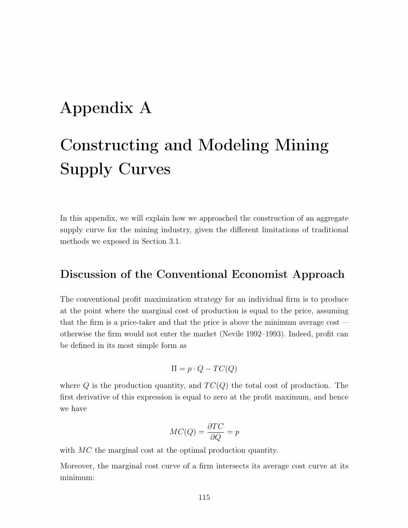
Appendix A

Constructing and Modeling Mining

Supply Curves

In this appendix, we will explain how we approached the construction of an aggregatesupply curve for the mining industry, given the different limitations of traditionalmethods we exposed in Section 3.1.

Discussion of the Conventional Economist Approach

The conventional profit maximization strategy for an individual firm is to produceat the point where the marginal cost of production is equal to the price, assumingthat the firm is a price-taker and that the price is above the minimum average cost —otherwise the firm would not enter the market (Nevile 1992–1993). Indeed, profit canbe defined in its most simple form as

⇧ = p ·Q� TC(Q)

where Q is the production quantity, and TC(Q) the total cost of production. Thefirst derivative of this expression is equal to zero at the profit maximum, and hencewe have

MC(Q) =

@TC

@Q= p

with MC the marginal cost at the optimal production quantity.

Moreover, the marginal cost curve of a firm intersects its average cost curve at itsminimum:

115

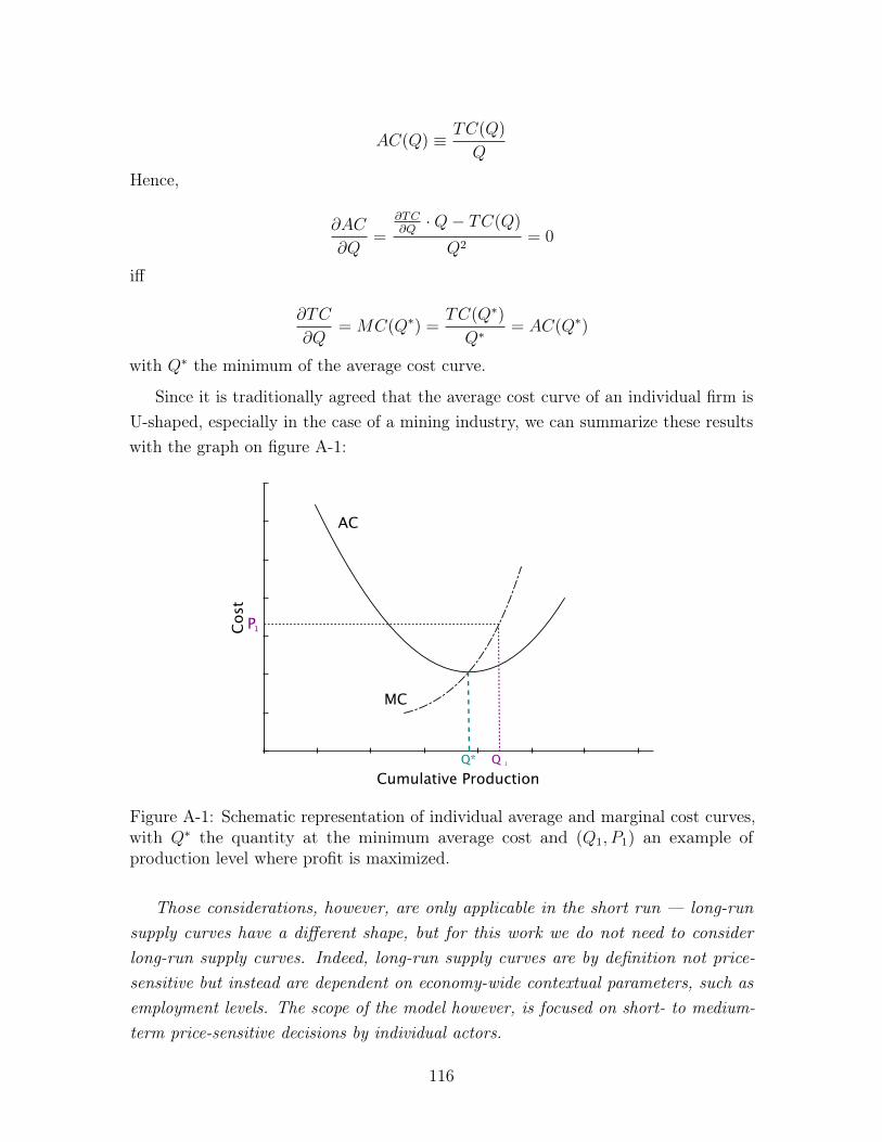
AC(Q) ⌘ TC(Q)

Q

Hence,

@AC

@Q=

@TC

@Q

·Q� TC(Q)

Q2= 0

iff

@TC

@Q= MC(Q⇤

) =

TC(Q⇤)

Q⇤ = AC(Q⇤)

with Q⇤ the minimum of the average cost curve.

Since it is traditionally agreed that the average cost curve of an individual firm isU-shaped, especially in the case of a mining industry, we can summarize these resultswith the graph on figure A-1:

Cumulative Production

Cos

t

AC

MC

Q* Q 1

P1

Figure A-1: Schematic representation of individual average and marginal cost curves,with Q⇤ the quantity at the minimum average cost and (Q1, P1) an example ofproduction level where profit is maximized.

Those considerations, however, are only applicable in the short run — long-runsupply curves have a different shape, but for this work we do not need to considerlong-run supply curves. Indeed, long-run supply curves are by definition not price-sensitive but instead are dependent on economy-wide contextual parameters, such asemployment levels. The scope of the model however, is focused on short- to medium-term price-sensitive decisions by individual actors.

116

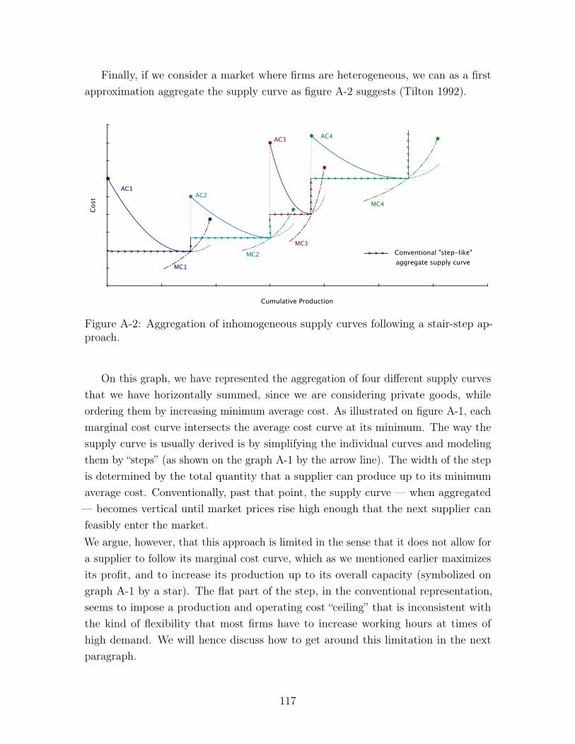
Finally, if we consider a market where firms are heterogeneous, we can as a firstapproximation aggregate the supply curve as figure A-2 suggests (Tilton 1992).

Cumulative Production

Cos

t

AC1

MC1

AC2

MC2

AC3

MC3

AC4

MC4

Conventional "step-like"aggregate supply curve

Figure A-2: Aggregation of inhomogeneous supply curves following a stair-step ap-proach.

On this graph, we have represented the aggregation of four different supply curvesthat we have horizontally summed, since we are considering private goods, whileordering them by increasing minimum average cost. As illustrated on figure A-1, eachmarginal cost curve intersects the average cost curve at its minimum. The way thesupply curve is usually derived is by simplifying the individual curves and modelingthem by “steps” (as shown on the graph A-1 by the arrow line). The width of the stepis determined by the total quantity that a supplier can produce up to its minimumaverage cost. Conventionally, past that point, the supply curve — when aggregated— becomes vertical until market prices rise high enough that the next supplier canfeasibly enter the market.We argue, however, that this approach is limited in the sense that it does not allow fora supplier to follow its marginal cost curve, which as we mentioned earlier maximizesits profit, and to increase its production up to its overall capacity (symbolized ongraph A-1 by a star). The flat part of the step, in the conventional representation,seems to impose a production and operating cost “ceiling” that is inconsistent withthe kind of flexibility that most firms have to increase working hours at times ofhigh demand. We will hence discuss how to get around this limitation in the nextparagraph.

117

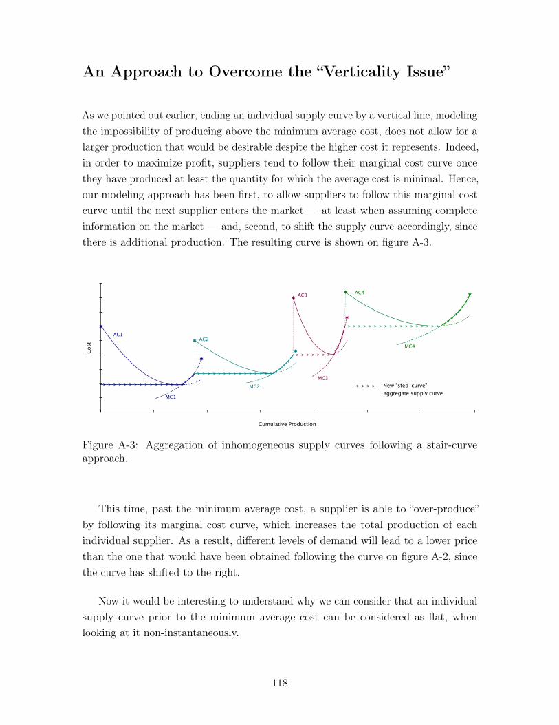
An Approach to Overcome the “Verticality Issue”

As we pointed out earlier, ending an individual supply curve by a vertical line, modelingthe impossibility of producing above the minimum average cost, does not allow for alarger production that would be desirable despite the higher cost it represents. Indeed,in order to maximize profit, suppliers tend to follow their marginal cost curve oncethey have produced at least the quantity for which the average cost is minimal. Hence,our modeling approach has been first, to allow suppliers to follow this marginal costcurve until the next supplier enters the market — at least when assuming completeinformation on the market — and, second, to shift the supply curve accordingly, sincethere is additional production. The resulting curve is shown on figure A-3.

Cumulative Production

Cos

t

AC1

MC1

AC2

MC2

AC3

MC3

AC4

MC4

New "step-curve"aggregate supply curve

Figure A-3: Aggregation of inhomogeneous supply curves following a stair-curveapproach.

This time, past the minimum average cost, a supplier is able to “over-produce”by following its marginal cost curve, which increases the total production of eachindividual supplier. As a result, different levels of demand will lead to a lower pricethan the one that would have been obtained following the curve on figure A-2, sincethe curve has shifted to the right.

Now it would be interesting to understand why we can consider that an individualsupply curve prior to the minimum average cost can be considered as flat, whenlooking at it non-instantaneously.

118

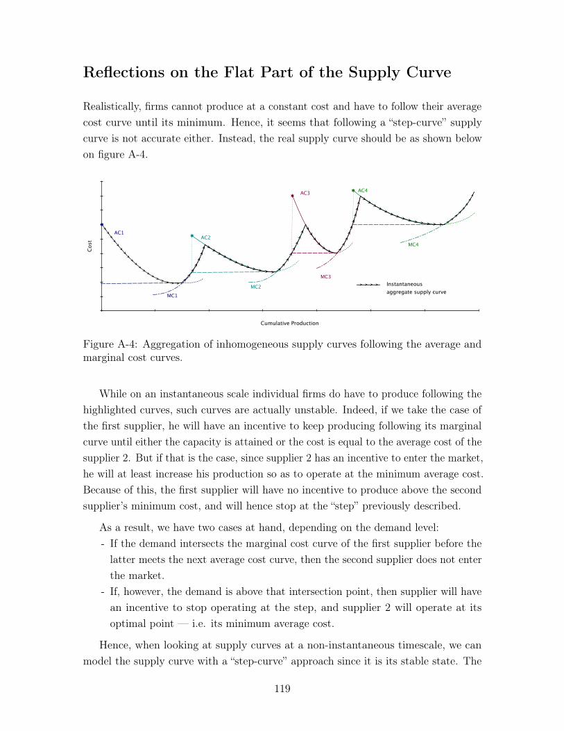
Reflections on the Flat Part of the Supply Curve

Realistically, firms cannot produce at a constant cost and have to follow their averagecost curve until its minimum. Hence, it seems that following a “step-curve” supplycurve is not accurate either. Instead, the real supply curve should be as shown belowon figure A-4.

Cumulative Production

Cos

t

AC1

MC1

AC2

MC2

AC3

MC3

AC4

MC4

Instantaneousaggregate supply curve

Figure A-4: Aggregation of inhomogeneous supply curves following the average andmarginal cost curves.

While on an instantaneous scale individual firms do have to produce following thehighlighted curves, such curves are actually unstable. Indeed, if we take the case ofthe first supplier, he will have an incentive to keep producing following its marginalcurve until either the capacity is attained or the cost is equal to the average cost of thesupplier 2. But if that is the case, since supplier 2 has an incentive to enter the market,he will at least increase his production so as to operate at the minimum average cost.Because of this, the first supplier will have no incentive to produce above the secondsupplier’s minimum cost, and will hence stop at the “step” previously described.

As a result, we have two cases at hand, depending on the demand level:- If the demand intersects the marginal cost curve of the first supplier before the

latter meets the next average cost curve, then the second supplier does not enterthe market.

- If, however, the demand is above that intersection point, then supplier will havean incentive to stop operating at the step, and supplier 2 will operate at itsoptimal point — i.e. its minimum average cost.

Hence, when looking at supply curves at a non-instantaneous timescale, we canmodel the supply curve with a “step-curve” approach since it is its stable state. The

119

curve depicted on figure A-3 is thus relevant in the short run, for non-instantaneousdecisions, which is appropriate in our study.

120

Appendix B

Derivation of the Supply Curves and

Interpolation of Marginal Cost

This appendix explains how the individual cost curves were constructed and, morespecifically, how the inverse function of the marginal cost curve — used to calculatethe production at each period as presented in Appendix C — was implemented.

Modeling Design Objectives

The general design objectives of the model in terms of supply curve algorithms havebeen as follows:

• The implementation of a relatively simple analytical functional form for thesupply curves that can still cover a wide range of behaviors in terms of supplyquantity and cost, while remaining easy to parametrize;

• Ensuring that the simulated average cost curves are U-shaped and have continu-ous first and second derivatives; and

• To use a functional form so that the marginal cost curve can be easily inverted,so that the level of production that a mine could achieve for a given price isreadily computable.

121

Derivation of the Average Cost Curve

Following standard microeconomic assumptions, the average cost curve of each minewas assumed to be ‘U-shaped’, with a clearly defined minimum. Mathematicalformulations satisfying this condition were employed to develop a general formula thatcould be parametrized to reflect a wide range of operating conditions.

Condition on the Second Derivative

The very first analytic condition the general cost curve must meet derives from thecondition that the second derivative of the average cost curve should be positive whenaverage cost is at a minimum, so that the marginal cost curve is upward-sloping whenit intersects the average cost curve. Starting with the definition of marginal cost:

MC(Q) =

@TC

@Q(B.1)

yet TC(Q) ⌘ AC(Q) ·Q by definition

hence MC(Q) = Q · @AC@Q

+ AC(Q) (B.2)

From the assumption stated above, the first derivative of the marginal cost should bepositive at Q⇤, the minimum average cost:

@MC(Q)

@Q

����Q

⇤> 0

ie@2AC

@Q2

����Q

⇤+ 2 · @AC

@Q

����Q

⇤> 0 (B.3)

By definition, @AC

@Q

��Q

⇤ = 0. The condition is hence

@2AC

@Q2

����Q

⇤> 0 (B.4)

While the condition given in Equation B.4 is only necessary at Q⇤, it can be generalizedto hold for the function generally, since it carries the desirable condition that theaverage cost function is convex.

122

Functional Form of the Average Cost Curve

The condition given in Equation B.4 on the second derivative, as explained in theprevious section, is the only condition required for initial modeling purposes. Whilemany functional forms can satisfy this condition, a pseudo-polynomial function fulfillingthe condition has been adopted, for it can be tuned depending on the mines and cancover a wide range of production quantities and costs:

@2AC

@Q2= a ·Qn (B.5)

where a > 0 and n � 0

Integrating Equation B.4 and using the following condition and formalism

@AC

@Q

����Q

⇤= 0

and

AC(Q⇤) = A⇤

lead to@AC

@Q=

a

n+ 1

·⇥Qn+1 � (Q⇤

)

n+1⇤ (B.6)

and

AC(Q) =

a

n+ 1

·Qn+2

n+ 2

� (Q⇤)

n+1 ·Q�+ A⇤

+

a

n+ 2

· (Q⇤)

n+2 (B.7)

Total cost and marginal cost hence become

TC(Q) =

a

n+ 1

·Qn+3

n+ 2

� (Q⇤)

n+1 ·Q2

�+

A⇤

+

a

n+ 2

· (Q⇤)

n+2

�·Q (B.8)

MC(Q) =

a

n+ 1

·n+ 3

n+ 2

·Qn+2 � 2 · (Q⇤)

n+1 ·Q�+ A⇤

+

a

n+ 2

· (Q⇤)

n+2 (B.9)

Equations B.8 and B.9 yield an analytic form that can be used to compute totaland marginal cost for a mine, given appropriate parameters, over the entire rangeof possible mine outputs. For modeling purposes, an explicit way of calculating theinverse function of the marginal cost is required in order to be able to compute theoutput of each mine at a given market price, which must be greater than or equal to

123

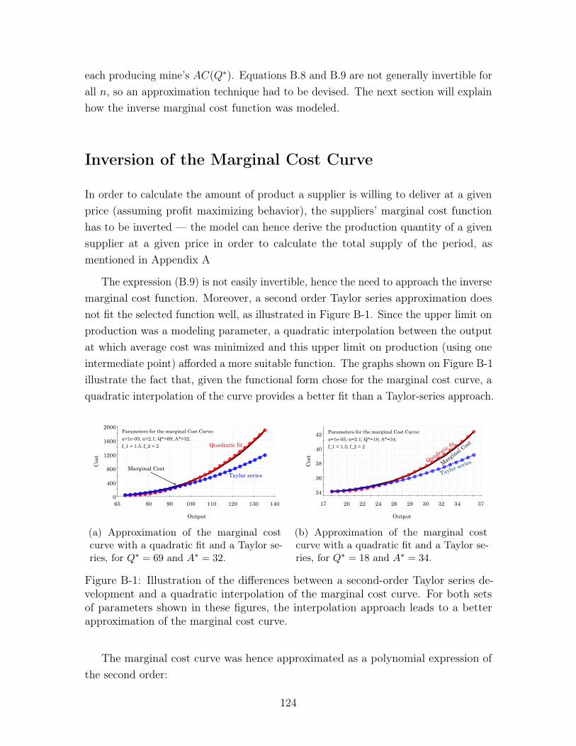
each producing mine’s AC(Q⇤). Equations B.8 and B.9 are not generally invertible for

all n, so an approximation technique had to be devised. The next section will explainhow the inverse marginal cost function was modeled.

Inversion of the Marginal Cost Curve

In order to calculate the amount of product a supplier is willing to deliver at a givenprice (assuming profit maximizing behavior), the suppliers’ marginal cost functionhas to be inverted — the model can hence derive the production quantity of a givensupplier at a given price in order to calculate the total supply of the period, asmentioned in Appendix A

The expression (B.9) is not easily invertible, hence the need to approach the inversemarginal cost function. Moreover, a second order Taylor series approximation doesnot fit the selected function well, as illustrated in Figure B-1. Since the upper limit onproduction was a modeling parameter, a quadratic interpolation between the outputat which average cost was minimized and this upper limit on production (using oneintermediate point) afforded a more suitable function. The graphs shown on Figure B-1illustrate the fact that, given the functional form chose for the marginal cost curve, aquadratic interpolation of the curve provides a better fit than a Taylor-series approach.

14065 80 90 100 110 120 130

2000

0

400

800

1200

1600

Output

Cos

t

Marginal Cost

Parameters for the marginal Cost Curve:

a=1e-05; n=2.1; Q*=69; A*=32;

f_1 = 1.5; f_2 = 2

Taylor series

Quadratic fit

(a) Approximation of the marginal costcurve with a quadratic fit and a Taylor se-ries, for Q

⇤ = 69 and A

⇤ = 32.

3717 20 22 24 26 28 30 32 34

34

36

38

40

42

Output

Cos

t

Marginal Cost

Taylor seriesQuadratic fit

Parameters for the marginal Cost Curve:

a=1e-05; n=2.1; Q*=18; A*=34;

f_1 = 1.5; f_2 = 2

(b) Approximation of the marginal costcurve with a quadratic fit and a Taylor se-ries, for Q

⇤ = 18 and A

⇤ = 34.

Figure B-1: Illustration of the differences between a second-order Taylor series de-velopment and a quadratic interpolation of the marginal cost curve. For both setsof parameters shown in these figures, the interpolation approach leads to a betterapproximation of the marginal cost curve.

The marginal cost curve was hence approximated as a polynomial expression ofthe second order:

124

gMC(Q) = a ·Q2+ b ·Q+ c (B.10)

such that gMC(Q⇤) = A⇤ (B.11)

gMC(f1 ·Q⇤) = MC(f1 ·Q⇤

) = M1 (B.12)gMC(f2 ·Q⇤

) = MC(f2 ·Q⇤) = M2 (B.13)

with 1 < f1 < f2

This approach uses “generic” interpolation points (given by f1 and f2) since f2 isalso the factor defining the upper limit of production at each period as a multipleof Q⇤. While producers are able to extract more material — at a higher cost thanthe lowest average cost point — there is still a physical capacity constraint in theshort-term production (Tilton 1992).

In general, we rarely observe a mine operating at twice its rated production capacity,but it can vary from mine to mine — a bigger mine may for instance be able to takeon a larger portion of “over”-production compared to a smaller mine that hence wouldhave a smaller f2. Those parameters have been made flexible, and can even vary overtime as the mine slowly depletes.

The three parameters a, b and c of the expression (B.10) can hence be derived,since there are three equations — namely (B.11), (B.12) and (B.13) — and threeunknown parameters:

a =

1

Q⇤ 2 · 1

f2 � f1· M2 � A⇤

f2 � 1

� M1 � A⇤

f1 � 1

!(B.14)

b and c can be inferred from this expression:

b =1

Q⇤ ·M2 � A⇤ �

�f 22 � 1

�· (Q⇤

)

2 · af2 � 1

(B.15)

c = A⇤ � (Q⇤)

2 · a�Q⇤ · b (B.16)

Once those parameters implemented, the quantity produced at a specific marginalcost of production can be easily inferred by using the Quadratic Formula, given theexpression (B.10) and the fact that we only want a positive production quantity:

125

Q =

�b+pb2 � 4 · a · c2 · a (B.17)

126

Appendix C

Simulation Strategies

The simulation strategy employed in the dynamic market model is built upon the notionthat the market is driven by suppliers independently making production decisionsbased on apparent price.

Calculation of production for operating mines

1. Start with a given price from the preceding time period, Pt�1

2. If Pt�1 � A⇤

i

for the i-th supplier, compute the quantity the i-th supplier willproduce, MC�1

(Pt�1), as illustrated on Figure C-1. Note that, because of

computational complexity, this inverse function is typically an approximation(refer to Appendix C).

3. Sum over all suppliers to get the supply in the current period, i.e., for all i suchthat P

t�1 � A⇤i

;P

i

MC�1i

(Pt�1) = S

t

.

Price-setting mechanism adopted by a market-maker

A market maker with perfect knowledge of the supply curve could take this approach:

1. Given demand at time t, Dt

2. Find the cost at which ideal supply equals demand:

(a) Order the suppliers in ascending order of A⇤

127

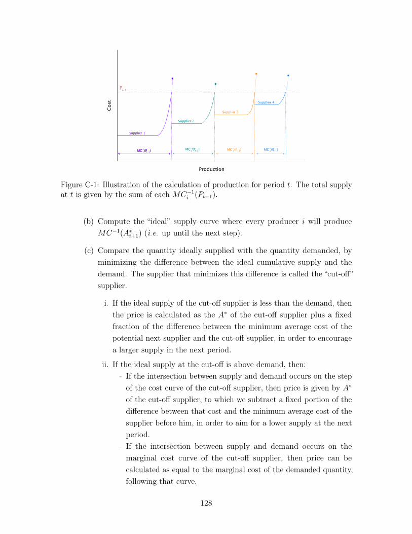
Production

Cost

Pt-1

Supplier 1

Supplier 2

Supplier 3

Supplier 4

MC (P )1 t-1-1 MC (P )2 t-1

-1MC (P ) MC (P )3 t-1-1 MC (P )4 t-1

-1

Figure C-1: Illustration of the calculation of production for period t. The total supplyat t is given by the sum of each MC�1

i

(Pt�1).

(b) Compute the “ideal” supply curve where every producer i will produceMC�1

(A⇤i+1) (i.e. up until the next step).

(c) Compare the quantity ideally supplied with the quantity demanded, byminimizing the difference between the ideal cumulative supply and thedemand. The supplier that minimizes this difference is called the “cut-off”supplier.

i. If the ideal supply of the cut-off supplier is less than the demand, thenthe price is calculated as the A⇤ of the cut-off supplier plus a fixedfraction of the difference between the minimum average cost of thepotential next supplier and the cut-off supplier, in order to encouragea larger supply in the next period.

ii. If the ideal supply at the cut-off is above demand, then:- If the intersection between supply and demand occurs on the step

of the cost curve of the cut-off supplier, then price is given by A⇤

of the cut-off supplier, to which we subtract a fixed portion of thedifference between that cost and the minimum average cost of thesupplier before him, in order to aim for a lower supply at the nextperiod.

- If the intersection between supply and demand occurs on themarginal cost curve of the cut-off supplier, then price can becalculated as equal to the marginal cost of the demanded quantity,following that curve.

128

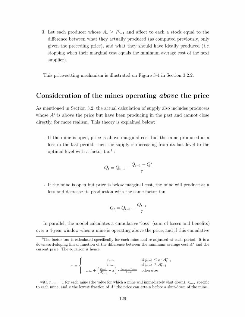
3. Let each producer whose A⇤ � Pt�1 and affect to each a stock equal to the

difference between what they actually produced (as computed previously, onlygiven the preceding price), and what they should have ideally produced (i.e.stopping when their marginal cost equals the minimum average cost of the nextsupplier).

This price-setting mechanism is illustrated on Figure 3-4 in Section 3.2.2.

Consideration of the mines operating above the price

As mentioned in Section 3.2, the actual calculation of supply also includes producerswhose A⇤ is above the price but have been producing in the past and cannot closedirectly, for more realism. This theory is explained below:

- If the mine is open, price is above marginal cost but the mine produced at aloss in the last period, then the supply is increasing from its last level to theoptimal level with a factor tau1 :

Qt

= Qt�1 �

Qt�1 �Q⇤

⌧

- If the mine is open but price is below marginal cost, the mine will produce at aloss and decrease its production with the same factor tau:

Qt

= Qt�1 �

Qt�1

⌧

In parallel, the model calculates a cumulative “loss” (sum of losses and benefits)over a 4-year window when a mine is operating above the price, and if this cumulative

1The factor tau is calculated specifically for each mine and re-adjusted at each period. It is adownward-sloping linear function of the difference between the minimum average cost A

⇤ and thecurrent price. The equation is hence:

⌧ =

8><

>:

⌧

min

if pt�1 x ·A⇤

t�1

⌧

max

if pt�1 � A

⇤t�1

⌧

min

+⇣

p

t�1

A

⇤t�1

� x

⌘· ⌧

max

�⌧

min

1�x

otherwise

with ⌧

min

= 1 for each mine (the value for which a mine will immediately shut down), ⌧max

specificto each mine, and x the lowest fraction of A⇤ the price can attain before a shut-down of the mine.

129

loss exceeds a certain factor (specific to each mine) times the “optimal” revenue Q⇤ ·A⇤,then the mine shuts down.

Finally, a process runs to monitor closings and openings of mines. In particular,mines that have not yet opened will only operate after a certain number of periods(monitored by the user on the inputs page) where the price is above its projectedminimum average cost.

130

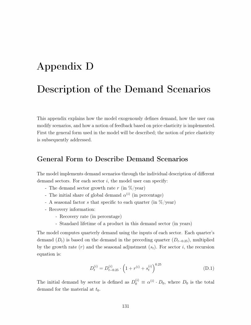
Appendix D

Description of the Demand Scenarios

This appendix explains how the model exogenously defines demand, how the user canmodify scenarios, and how a notion of feedback based on price elasticity is implemented.First the general form used in the model will be described; the notion of price elasticityis subsequently addressed.

General Form to Describe Demand Scenarios

The model implements demand scenarios through the individual description of differentdemand sectors. For each sector i, the model user can specify:

- The demand sector growth rate r (in %/year)- The initial share of global demand ↵(i) (in percentage)- A seasonal factor s that specific to each quarter (in %/year)- Recovery information:

- Recovery rate (in percentage)- Standard lifetime of a product in this demand sector (in years)

The model computes quarterly demand using the inputs of each sector. Each quarter’sdemand (D

t

) is based on the demand in the preceding quarter (Dt�0.25), multiplied

by the growth rate (r) and the seasonal adjustment (st

). For sector i, the recursionequation is:

D(i)t

= D(i)t�0.25 ·

⇣1 + r(i) + s

(i)t

⌘0.25(D.1)

The initial demand by sector is defined as D(i)0 ⌘ ↵(i) · D0, where D0 is the total

demand for the material at t0.

131

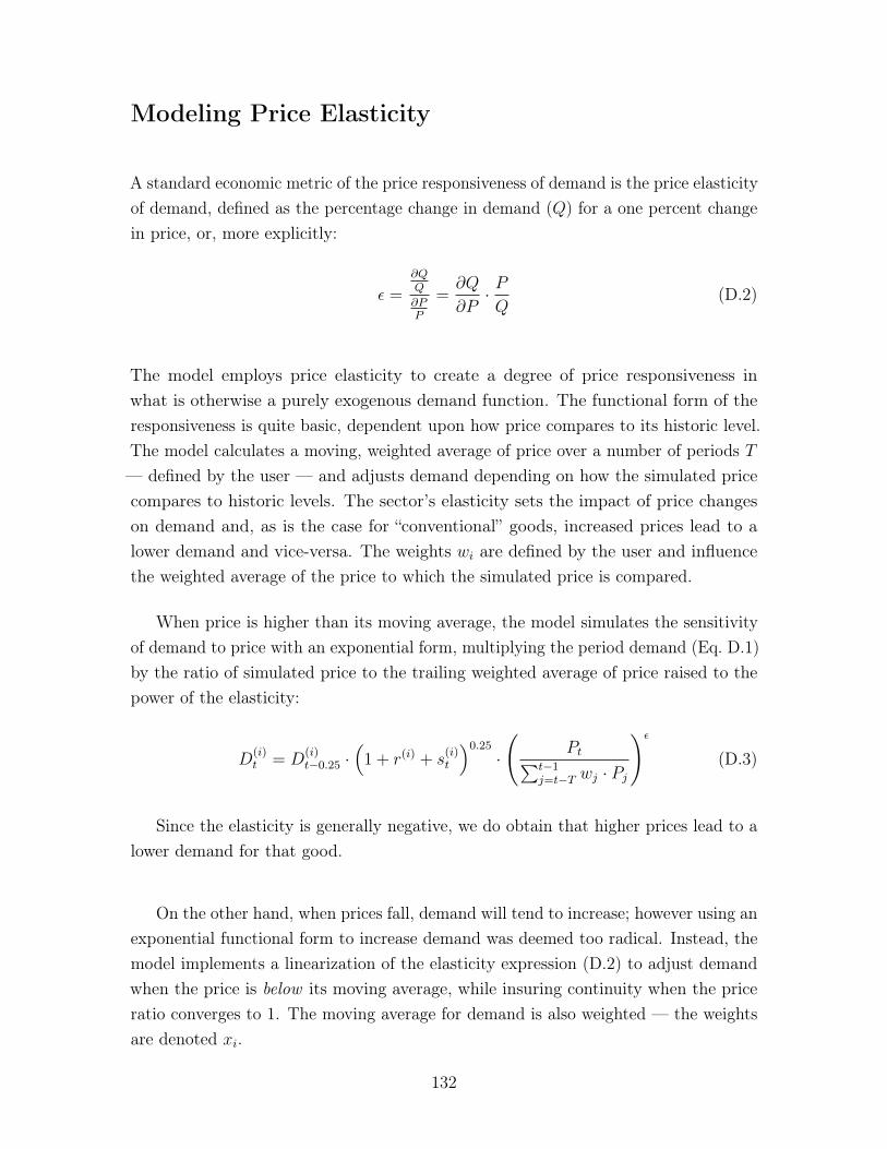
Modeling Price Elasticity

A standard economic metric of the price responsiveness of demand is the price elasticityof demand, defined as the percentage change in demand (Q) for a one percent changein price, or, more explicitly:

✏ =

@Q

Q

@P

P

=

@Q

@P· PQ

(D.2)

The model employs price elasticity to create a degree of price responsiveness inwhat is otherwise a purely exogenous demand function. The functional form of theresponsiveness is quite basic, dependent upon how price compares to its historic level.The model calculates a moving, weighted average of price over a number of periods T

— defined by the user — and adjusts demand depending on how the simulated pricecompares to historic levels. The sector’s elasticity sets the impact of price changeson demand and, as is the case for “conventional” goods, increased prices lead to alower demand and vice-versa. The weights w

i

are defined by the user and influencethe weighted average of the price to which the simulated price is compared.

When price is higher than its moving average, the model simulates the sensitivityof demand to price with an exponential form, multiplying the period demand (Eq. D.1)by the ratio of simulated price to the trailing weighted average of price raised to thepower of the elasticity:

D(i)t

= D(i)t�0.25 ·

⇣1 + r(i) + s

(i)t

⌘0.25·

PtP

t�1j=t�T

wj

· Pj

!✏

(D.3)

Since the elasticity is generally negative, we do obtain that higher prices lead to alower demand for that good.

On the other hand, when prices fall, demand will tend to increase; however using anexponential functional form to increase demand was deemed too radical. Instead, themodel implements a linearization of the elasticity expression (D.2) to adjust demandwhen the price is below its moving average, while insuring continuity when the priceratio converges to 1. The moving average for demand is also weighted — the weightsare denoted x

i

.

132

✏ =

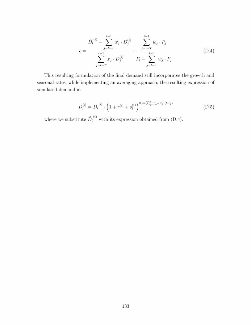
˜Dt

(i) �t�1X

j=t�T

xj

·D(i)j

t�1X

j=t�T

xj

·D(i)j

·

t�1X

j=t�T

wj

· Pj

Pt

�t�1X

j=t�T

wj

· Pj

(D.4)

This resulting formulation of the final demand still incorporates the growth andseasonal rates, while implementing an averaging approach; the resulting expression ofsimulated demand is:

D(i)t

=

˜Dt

(i) ·⇣1 + r(i) + s

(i)t

⌘0.25·Pt�1j=t�T xj ·(t�j)

(D.5)

where we substitute ˜Dt

(i) with its expression obtained from (D.4).

133

134

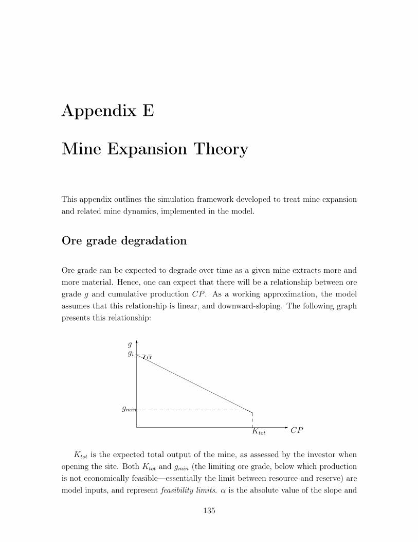
Appendix E

Mine Expansion Theory

This appendix outlines the simulation framework developed to treat mine expansionand related mine dynamics, implemented in the model.

Ore grade degradation

Ore grade can be expected to degrade over time as a given mine extracts more andmore material. Hence, one can expect that there will be a relationship between oregrade g and cumulative production CP . As a working approximation, the modelassumes that this relationship is linear, and downward-sloping. The following graphpresents this relationship:

-

6

HHHHHHHHHHHHHHHHHHgmin

gi

g

CPKtot

↵

Ktot

is the expected total output of the mine, as assessed by the investor whenopening the site. Both K

tot

and gmin

(the limiting ore grade, below which productionis not economically feasible—essentially the limit between resource and reserve) aremodel inputs, and represent feasibility limits. ↵ is the absolute value of the slope and

135

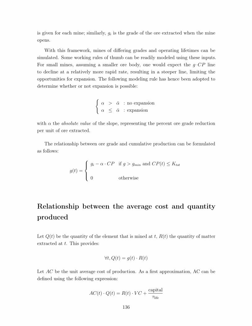
is given for each mine; similarly, gi

is the grade of the ore extracted when the mineopens.

With this framework, mines of differing grades and operating lifetimes can besimulated. Some working rules of thumb can be readily modeled using these inputs.For small mines, assuming a smaller ore body, one would expect the g–CP lineto decline at a relatively more rapid rate, resulting in a steeper line, limiting theopportunities for expansion. The following modeling rule has hence been adopted todetermine whether or not expansion is possible:

(↵ > ↵̄ : no expansion↵ ↵̄ : expansion

with ↵ the absolute value of the slope, representing the percent ore grade reductionper unit of ore extracted.

The relationship between ore grade and cumulative production can be formulatedas follows:

g(t) =

8><

>:

gi

� ↵ · CP if g > gmin

and CP (t) Ktot

0 otherwise

Relationship between the average cost and quantityproduced

Let Q(t) be the quantity of the element that is mined at t, R(t) the quantity of matterextracted at t. This provides:

8t, Q(t) = g(t) ·R(t)

Let AC be the unit average cost of production. As a first approximation, AC can bedefined using the following expression:

AC(t) ·Q(t) = R(t) · V C +

capital⌧life

136

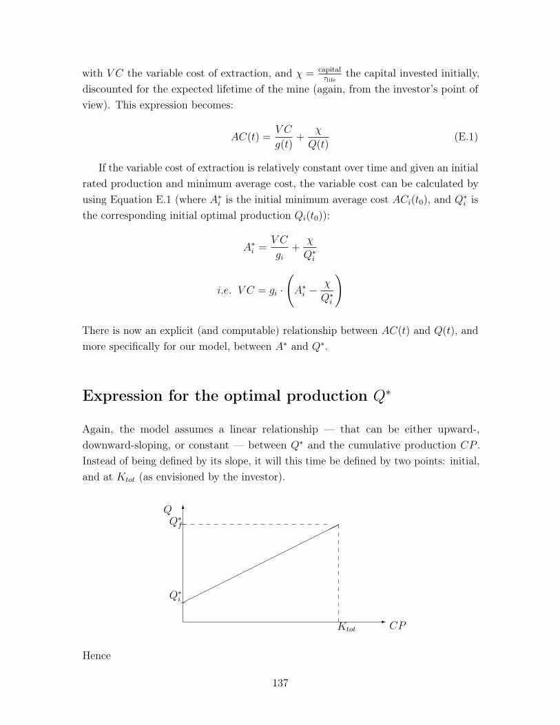
with V C the variable cost of extraction, and � =

capital

⌧lifethe capital invested initially,

discounted for the expected lifetime of the mine (again, from the investor’s point ofview). This expression becomes:

AC(t) =V C

g(t)+

�

Q(t)(E.1)

If the variable cost of extraction is relatively constant over time and given an initialrated production and minimum average cost, the variable cost can be calculated byusing Equation E.1 (where A⇤

i

is the initial minimum average cost ACi

(t0), and Q⇤i

isthe corresponding initial optimal production Q

i

(t0)):

A⇤i

=

V C

gi

+

�

Q⇤i

i.e. V C = gi

· A⇤

i

� �

Q⇤i

!

There is now an explicit (and computable) relationship between AC(t) and Q(t), andmore specifically for our model, between A⇤ and Q⇤.

Expression for the optimal production Q⇤

Again, the model assumes a linear relationship — that can be either upward-,downward-sloping, or constant — between Q⇤ and the cumulative production CP .Instead of being defined by its slope, it will this time be defined by two points: initial,and at K

tot

(as envisioned by the investor).

-

6

������������������

Q⇤i

Q⇤f

Q

CPKtot

Hence

137

Q(t) = Q⇤i

+

Q⇤f

�Q⇤i

Ktot

· CP (t)

Now Q⇤f

should be calculated. From the assumption that the investor envisionsa production at Q⇤

(t) at each period, Q can be replaced by Q⇤. Moreover, CP (t) =Rt

tiQ(t)dt.

Deriving the expression for Q(t) once with respect to t, we obtain a first-order lineardifferential equation:

@Q⇤

@t=

Q⇤f

�Q⇤i

Ktot

·Q⇤(t)

The solution is hence:

Q⇤(t) = Q⇤

i

· exp Q⇤

f

�Q⇤i

Ktot

· t!

Finally, at t = ⌧life

, we have Q⇤(⌧

life

) = Q⇤f

. The following equation provides a meansto calculate Q⇤

f

:

lnQ⇤f

� lnQ⇤i

Q⇤f

�Q⇤i

=

⌧life

Ktot

Using the function Goal Seek in Excel®, Q⇤f

can be estimated numerically withinthe model.

Derivation of the minimum average cost A⇤

Given the expression (E.1), A⇤(t) can be derived from the calculation of Q⇤

(t) bysimply applying this formula to the point where the average cost is minimal, and wehence obtain:

A⇤(t) =

V C

g(t)+

�

Q⇤(t)

This mine dynamics approach is implemented in the model and is used to account formine expansion when running simulations over several years.

138

Bibliography

Abraham, David (Mar. 2012). “The Battle for New Resources: Minor minerals ingreen technologies”. In: RIETI Policy Discussion Papers 12-P-005.

Allison, Graham T. (Sept. 1969). “Conceptual Models and the Cuban Missile Crisis”.In: The American Political Science Review 63.3, pp. 689–718.

Alonso, Elisa (2010). “Materials Scarcity from the Perspective of Manufacturing Firms:Case Studies of Platinum and Cobalt”. Doctor of Philosophy in MaterialsScience and Engineering. Massachusetts Institute of Technology. 216 pp.

Banks Ferdinand, E. (June 1983). “Primary commodity prices — a pedagogical note”.In: Resources Policy 9.2, pp. 141–142. doi: 10.1016/0301-4207(83)90055-7.

Bauer, Diana et al. (2011). Critical Materials Strategy. Office of Policy and InternationalAffairs. U.S. Department of Energy. url: http://energy.gov/sites/prod/files/DOE_CMS2011_FINAL_Full.pdf.

Bradsher, Keith (Nov. 2010). “China Restarts Rare Earth Shipments to Japan”. In:The New York Times (The New York Edition). url: http://www.nytimes.com/2010/11/20/business/global/20rare.html?_r=0.

Busch, Marc (1999). Trade Warriors – States, Firms, and Strategic-Trade Policy inHigh-Technology Competition. Cambridge University Press.

Chapman, P.F. and F. Roberts (Apr. 1983). Metal Resources and Energy. Butterworth-Heinemann Ltd.

China’s Rare Earth Industry and Export Regime: Economic and Trade Implicationsfor the United States (2012). Report for Congress. Congressional ResearchService.

Cohen, Kalman J. et al. (Apr. 1981). “Transaction Costs, Order Placement Strategy,and Existence of the Bid-Ask Spread”. In: Journal of Political Economy 89.2,pp. 287–305.

139

Critical Raw Materials for the EU (2010). Report of the ad-hoc working group ondefining critical raw materials. European Commission.

Dasgupta, Partha and Geoffrey Heal (1974). “The Optimal Depletion of ExhaustibleResources”. In: The Review of Economic Studies. Symposium on the Economicsof Exhaustible Resources 3.28. Ed. by The Review of Economic Studies Ltd.

Deng, Xiaoping (1986). Program 863. National High-Tech R&D Program. Scienceand Technology Program. Ministry of Science and Technology of the People’sRepublic of China. url: http://web.archive.org/web/20130326102142/http://www.most.gov.cn/eng/programmes1/200610/t20061009_36225.htm.

Devarajan, Shantayanan and Anthony C. Fisher (Mar. 1981). “Hotelling’s "Eco-nomics of Exhaustible Resources": Fifty Years Later”. In: Journal of EconomicLiterature 19.1, pp. 65–73.

Dodd-Frank Act (2010) (Jan. 2010). Dodd-Frank Wall Street Reform and ConsumerProtection Act. Congress of the United States of America. Chap. Title XV,Sec. 1502.

Eggert, R. et al. (2008). Minerals, critical minerals, and the U.S. economy. NationalResearch Council (U.S.)

Eggert, Roderick G. (June 1991). “An empirical and conceptual introduction”. In:Resources Policy 17.2, pp. 91–99. doi: 10.1016/0301-4207(91)90033-R.

Erdman, L. and T.E. Graedel (Aug. 2011). “Criticality of Non-Fuel Minerals: a Reviewof Major Approaches and Analyses”. In: Environmental Science and Technology45, pp. 7620–7630.

Garman, Mark B. (June 1976). “Market microstructure”. In: Journal of FinancialEconomics 3 (3), pp. 257–275.

Gordon, R. B., M. Bertram, and T. E. Graedel (2006). “Metal stocks and sustainability”.In: Proceedings of the National Academy of Sciences of the United States ofAmerica 103.5, pp. 1209–1214.

Graedel, T et al. (Dec. 2011). “Methodology of Metal Criticality Determination”. In:Environmental Science and Technology 10.1021.

Grossman, S (June 1980). “On the Impossibility of Informationally Efficient Markets”.In: The American Economic Review 70 (3), pp. 393–408.

140

Hammond, Kenneth R. (1996). Human Judgment and Social Policy: Irreducible Un-certainty, Inevitable Error, Unavailable Injustice. New York: Oxford UniversityPress, p. 106.

Hartman, Howard L., ed. (1992). SME Mining Engineering Handbook. 2nd. Vol. 1.Littleton, Colorado: Society for Mining, Metallurgy, and Exploration, Inc. isbn:0-87335-100-2.

Hotelling, H (1931). “The Economics of Exhaustible Resources”. In: The Journal ofPolitical Economy 39 (2), pp. 137–175.

Hurst, Cindy (Mar. 2010). China’s Rare Earth Elements Industry: What Can theWest Learn? Institute for the Analysis of Global Security (IAGS).

Jaffe, R et al. (2011). Energy Critical Elements: Securing Materials for Emerging Tech-nologies. Panel on Public Affairs and the Materials Research Society’s Govern-ment Affairs Committee. APS. url: http://www.aps.org/policy/reports/popa-reports/loader.cfm?csModule=security/getfile&PageID=236337.

Johnson Matthey. PGMs Market data tables. url: http://www.platinum.matthey.com/publications/market-data-tables/. last checked on May 6th 2013 at2:46pm.

Kmenta, Jan and Roy F. Gilbert (1968). “Small Sample Properties of AlternativeEstimators of Seemingly Unrelated Regressions”. In: Journal of the AmericanStatistical Association 63.324, pp. 1180–1200.

Koopmans, Tjalling C. (Apr. 1949). “Identification Problems in Economic ModelConstruction”. In: Econometrica 17.2, pp. 125–144.

Krueger, Anne O. (June 1974). “The Political Economy of the Rent-Seeking Society”.In: The American Economic Review 64.3, pp. 291–303.

Labys, Walter C., J. B. Lesourd, and D. Badillo (1998). “Existence of metal pricecycles”. In: Resources Policy 24.3, pp. 147–155.

Malthus, Thomas (1798). An Essay on the Principle of Population. An Essay on thePrinciple of Population, as it Affects the Future Improvement of Society withRemarks on the Speculations of Mr. Godwin, M. Condorcet, and Other Writers.London.

Meadows, Donella H. et al. (1972). The Limits to growth; a report for the Club ofRome’s project on the predicament of mankind. 1st. New York: Universe Books,p. 60.

141

Morrison, Wayne M. and Rachel Tang (Apr. 2012). China’s Rare Earth Industry andExport Regime: Economic and Trade Implications for the United States. CRSReport for Congress. Congressional Research Service.

Nevile, J. W. (1992–1993). “Notes on Keynes’ Aggregate Suply Curve”. In: Journalof Post Keynesian Economics 15.2 (Winter), pp. 255–260. url: http://www.jstor.org/stable/4538338.

Olson, Mancur (1984). The Rise and Decline of Nations – Economic Growth, Stagfla-tion, and Social Rigidities. Yale University Press.

Pindyck, Robert S. (Oct. 1978). “Optimal Exploration and Production of a Non-Renewable Resource”. In: Journal of Political Economy 86.5. Ed. by TheUniversity of Chicago Press, pp. 841–861.

Rezaei, Jafar and Roland Ortt (2012). “A multi-variable approach to supplier seg-mentation”. In: International Journal of Production Research 50.16, pp. 4593–4611.

Scherer, Frederic M. and David Ross (1990). Industrial Market Structure and EconomicPerformance. 3rd.

Situation and Policies of China’s Rare Earth Industry (2010). Information Office ofthe State Council – The People’s Republic of China.

Solow, Robert M. (1956). “A Contribution to the Theory of Economic Growth”. In:The Quarterly Journal of Economics 70.1, pp. 65–94.

Stigler, George T. (Apr. 1964). “Public Regulation of the Securities Markets”. In: TheJournal of Business 37.2, pp. 117–142.

Stigler, Georges (1971). “The Theory of Economic Regulation”. In: The Bell Journalof Economics and Management Science 2.1, pp. 3–21.

Thomson Reuters GFMS (2013). Palladium Market Outlook. url: http://www.monex.com/gfms/2013/palladium-market-outlook-overview.html. lastchecked on May 6th 2013 at 2.46pm.

Tilton, John E. (1992). “Economics of the Mineral Industries”. In: SME MiningEngineering Handbook. Ed. by Howard L. Hartman. 2nd. Vol. 1. Littleton,Colorado: Society for Mining, Metallurgy, and Exploration, Inc. Chap. 2.1,pp. 47–62. isbn: 0-87335-100-2.

142

Torries Thomas, F. (Sept. 1988). “Competitive cost analysis in the mineral industries:The example of nickel”. In: Resources Policy 14.3, pp. 193–204. doi: 10.1016/0301-4207(88)90005-0.

United States Geological Survey. Platinum-Group Metals Statistics and Information.url: http://minerals.usgs.gov/minerals/pubs/commodity/platinum/.last checked on May 6th 2013 at 2:47pm.

Urbance, Randall J. (2001). “The Impact of Increased Automotive Interest on theWorld Magnesium Market: Dynamic Market SImulation”. Master of Sciencein Materials Science and Engineering. Massachusetts Institute of Technology.143 pp.

Urbance, Randall J. et al. (2002). “Economics: Market Model Simulation: The Impactof Increased Automotive Interest in Magnesium”. In: Journal of Minerals Metalsand Materials Society 54.8, pp. 25–33.

U.S. Department of Justice and The Federal Trade Commission (Aug. 2010). HorizontalMerger Guidelines. Tech. rep. Government of the United States of America.Chap. 5.3, pp. 18–19. url: http://web.archive.org/web/20130113154737/http://www.justice.gov/atr/public/guidelines/hmg-2010.pdf.

Yager, Thomas R., Yadira Soto-Viruet, and James J. Barry (2012). Recent Strikes inSouth Africa’s Platinum-Group Metal Mines: Effects Upon World Platinum-Group Metal Supplies. Open-File Report. Reston, Virginia: U.S. Departmentof the Interior and U.S. Geological Survey.

143