Conta t analysis and overlappingdomain de omposition methods fordynami and nonlinear problemsVon der Fakultät Mathematik und Physik der Universität Stuttgartzur Erlangung der Würde eines Doktors derNaturwissens haften (Dr. rer. nat.) genehmigte Abhandlung

Vorgelegt vonStephan Brunÿenaus Varel i.O.Hauptberi hter: Prof. Dr. B. WohlmuthMitberi hter: Prof. Dr. C. WienersProf. Dr. M. S häferTag der mündli hen Prüfung: 4. April 2008

Institut für Angewandte Analysis und Numeris he SimulationUniversität Stuttgart2008

D93 (Diss. Universität Stuttgart)

A knowledgmentsThis thesis summarizes the results of my resear h a tivities during the years 2003 to2008 at the hair `Numeris he Mathematik für Hö hstleistungsre hner' of the Institut fürAngewandte Analysis und Numeris he Simulation (IANS), Universität Stuttgart.The resear h work was funded by the German Resear h Foundation (DFG) whi h isgratefully a knowledged.I would like to express my extraordinary gratitude to my supervisor and a ademi tea herProf. Dr. Barbara Wohlmuth for her mentoring, support and enduring en ouragementof my work. Her outstanding dedi ation to the resear h a tivities of the whole group hasbeen truly inspiring for me. I would also like to thank her for giving me the opportunityto present my work on international onferen es.My spe ial thanks go to Prof. Dr. Christian Wieners and Prof. Dr. Mi hael S häfer fortheir eorts to provide the referee reports for this thesis. I am very grateful to Prof. Dr.Barbara Kaltenba her for parti ipating in the oral defense. I also would like to thank thes ientists with whom I had the pleasure to o-author several ontributions: Dr. MarkusBamba h, Prof. Dr. Gerhard Hirt and in parti ular Prof. Dr. Ekkehard Ramm andagain Prof. Dr. Mi hael S häfer.I thank Dr. Florian S hmid and Dr. Stefan Hartmann not only for writing publi ationswith me but also for their lose and very pleasant ollaboration.I am mu h obliged to the supervisors of my Diploma thesis Dr. Henning Behnke andProf. Dr. Ulri h Mertins for arousing my interest in the Finite Element method.Thanks to Dr. Paul Lyons and his o-workers for most stimulating dis ussions about onta t problems in an industrial ontext and also to Dr. Uwe-Jens Görke for his help onnite plasti ity. Thanks also to the LASSO GmbH for giving software te hni al support.During my employment at the IANS, I greatly enjoyed the inspiring and ooperativeatmosphere. I thank Dr. Andreas Klimke, Dr. Bishnu Lami hhane, Mi hael Mair, BritSteiner and Alexander Weiÿ for always being available and oering help and advi e fora omplishing the various theoreti al, te hni al and administrative tasks onne ted withthis thesis. I would espe ially like to thank Corinna Hager and Dr. Bernd Flemis h fortheir ooperation in domain de omposition methods and for proofreading parts of mythesis and Stefan Hüeber for his help on onta t problems.I am deeply indebted to my family and espe ially to my parents for always supporting mewith all their strength and goodwill. Finally I would like to express my deepest gratitudeto my wife Haixia for her onstant moral support and en ouragement. Without her loveand patien e, it would not have been possible to omplete this work.Stuttgart, April 2008 Stephan Brunÿeniii

ContentsAbstra t ixZusammenfassung xiNotations xiii1 Introdu tion 11.1 Deep-rolling . . . . . . . . . . . . . . . . . . . . . . . . . . . . . . . . . . 11.2 In remental sheet metal forming . . . . . . . . . . . . . . . . . . . . . . . 21.3 Aim and outline of this work . . . . . . . . . . . . . . . . . . . . . . . . 32 Classi al 1-grid dis retization: Plasti ity 72.1 Introdu tion . . . . . . . . . . . . . . . . . . . . . . . . . . . . . . . . . . 72.2 Governing equations and notations . . . . . . . . . . . . . . . . . . . . . 72.3 Global equilibrium iteration and Finite Element dis retization . . . . . . 82.4 A Gauss point se tion: Radial Return for linear isotropi hardening . . . 102.4.1 Consistent elastoplasti tangent module . . . . . . . . . . . . . . . 122.4.2 Plasti onsisten y parameter . . . . . . . . . . . . . . . . . . . . 132.5 A Gauss point se tion: The Tangent Cutting Plane algorithm . . . . . . 142.5.1 Fulllment of the yield ondition . . . . . . . . . . . . . . . . . . 162.5.2 Dis ussion . . . . . . . . . . . . . . . . . . . . . . . . . . . . . . . 172.6 A Gauss point se tion: Sequential quadrati programming . . . . . . . . 172.6.1 Denitions . . . . . . . . . . . . . . . . . . . . . . . . . . . . . . . 172.6.2 Derivation of the SQP step . . . . . . . . . . . . . . . . . . . . . . 182.6.3 The SQP step and the algorithm . . . . . . . . . . . . . . . . . . 182.7 Comparison of the Gauss point algorithms . . . . . . . . . . . . . . . . . 202.8 Numeri al results . . . . . . . . . . . . . . . . . . . . . . . . . . . . . . . 212.9 Some tensor al ulus . . . . . . . . . . . . . . . . . . . . . . . . . . . . . 232.10 Summary . . . . . . . . . . . . . . . . . . . . . . . . . . . . . . . . . . . 233 Classi al 1-grid dis retization: Conta t 253.1 Conta t algorithms in the literature . . . . . . . . . . . . . . . . . . . . 253.2 The primal dual a tive set strategy with dual Lagrange multipliers . . . . 273.2.1 Basi idea . . . . . . . . . . . . . . . . . . . . . . . . . . . . . . . 273.2.2 Continuous equations . . . . . . . . . . . . . . . . . . . . . . . . 283.2.3 A tive Set Strategy and Algebrai Multigrid Methods . . . . . . . 313.2.4 Dis retized form . . . . . . . . . . . . . . . . . . . . . . . . . . . 32v

Contents3.2.5 Nonlinear algorithm for 1-grid dis retization . . . . . . . . . . . . 333.2.6 Inexa t strategy . . . . . . . . . . . . . . . . . . . . . . . . . . . 363.3 Numeri al results for onta t . . . . . . . . . . . . . . . . . . . . . . . . 363.3.1 Blo k indention test . . . . . . . . . . . . . . . . . . . . . . . . . 363.3.2 Comparison of both onta t approa hes in onne tion with AMG 373.3.3 A tive set versus adaptive penalty strategies . . . . . . . . . . . . 383.3.4 A eleration by AMG-inexa t strategy . . . . . . . . . . . . . . . 403.4 Summary . . . . . . . . . . . . . . . . . . . . . . . . . . . . . . . . . . . 424 Dynami onta t 434.1 Introdu tion . . . . . . . . . . . . . . . . . . . . . . . . . . . . . . . . . . 434.2 Problem des ription . . . . . . . . . . . . . . . . . . . . . . . . . . . . . 444.2.1 One-body onta t with rigid obsta le . . . . . . . . . . . . . . . . 444.2.2 Boundary value problem of nonlinear elastodynami s . . . . . . . 464.3 Spatial dis retization of onta t virtual work . . . . . . . . . . . . . . . 464.3.1 Dis rete dual Lagrange multipliers for arbitrary shaped elements . 474.3.2 Semidis rete initial value problem . . . . . . . . . . . . . . . . . . 494.4 Time dis retization . . . . . . . . . . . . . . . . . . . . . . . . . . . . . . 504.4.1 Linearization and iterative solution strategy . . . . . . . . . . . . 514.4.2 Global system with onta t manipulation . . . . . . . . . . . . . 524.5 Spatial dis retization by a nite shell element . . . . . . . . . . . . . . . 534.6 Energy onservation for fri tionless onta t . . . . . . . . . . . . . . . . 534.7 Examples . . . . . . . . . . . . . . . . . . . . . . . . . . . . . . . . . . . 564.7.1 Weak non-penetration . . . . . . . . . . . . . . . . . . . . . . . . 574.7.2 Toss rule . . . . . . . . . . . . . . . . . . . . . . . . . . . . . . . . 574.7.3 Ball . . . . . . . . . . . . . . . . . . . . . . . . . . . . . . . . . . 604.7.4 Torus . . . . . . . . . . . . . . . . . . . . . . . . . . . . . . . . . 614.8 Con lusions . . . . . . . . . . . . . . . . . . . . . . . . . . . . . . . . . . 625 Velo ity based onta t problems 656 Coupling algorithm 716.1 Dynami ODDM, main on epts . . . . . . . . . . . . . . . . . . . . . . 716.2 Review of the literature . . . . . . . . . . . . . . . . . . . . . . . . . . . 736.3 Coupling s heme . . . . . . . . . . . . . . . . . . . . . . . . . . . . . . . 746.3.1 Fine domain . . . . . . . . . . . . . . . . . . . . . . . . . . . . . 756.3.2 Coarse domain . . . . . . . . . . . . . . . . . . . . . . . . . . . . 756.3.3 Solving the nonlinear problem with a oarse global and a ne lo almesh . . . . . . . . . . . . . . . . . . . . . . . . . . . . . . . . . 776.4 Numeri al results . . . . . . . . . . . . . . . . . . . . . . . . . . . . . . . 796.4.1 Material data . . . . . . . . . . . . . . . . . . . . . . . . . . . . . 796.4.2 Elasti example, non-hierar hi al ase . . . . . . . . . . . . . . . 796.4.3 Numeri al testing of the mortar operator . . . . . . . . . . . . . . 806.4.4 Relative error . . . . . . . . . . . . . . . . . . . . . . . . . . . . . 84vi

Contents6.4.5 Update strategies . . . . . . . . . . . . . . . . . . . . . . . . . . 866.4.6 Deep-rolling like example . . . . . . . . . . . . . . . . . . . . . . . 876.5 Con lusions and future work . . . . . . . . . . . . . . . . . . . . . . . . 877 An inexa t Newton blo k s heme 917.1 Motivation . . . . . . . . . . . . . . . . . . . . . . . . . . . . . . . . . . . 917.2 Blo k iterative s heme: Linear elasti ity . . . . . . . . . . . . . . . . . . 917.3 Newton Blo k iterative s heme: Elasti ity with onta t . . . . . . . . . . 937.4 Newton Blo k iterative s heme: Plasti ity with onta t . . . . . . . . . . 947.5 Blo k iterative s hemes . . . . . . . . . . . . . . . . . . . . . . . . . . . . 967.6 S hur omplement method . . . . . . . . . . . . . . . . . . . . . . . . . . 967.6.1 S hur omplement method, elasti ase . . . . . . . . . . . . . . 967.6.2 S hur omplement method, plasti ase . . . . . . . . . . . . . . . 987.7 Inexa t Newton methods . . . . . . . . . . . . . . . . . . . . . . . . . . 997.7.1 Avoiding oversolving . . . . . . . . . . . . . . . . . . . . . . . . . 997.7.2 Iterative solver . . . . . . . . . . . . . . . . . . . . . . . . . . . . 997.8 Complete algorithm . . . . . . . . . . . . . . . . . . . . . . . . . . . . . . 1017.9 Numeri al results . . . . . . . . . . . . . . . . . . . . . . . . . . . . . . . 1017.9.1 Model example . . . . . . . . . . . . . . . . . . . . . . . . . . . . 1017.9.2 S hur omplement method . . . . . . . . . . . . . . . . . . . . . . 1027.9.3 Blo k Gauss Seidel . . . . . . . . . . . . . . . . . . . . . . . . . . 1027.10 Summary . . . . . . . . . . . . . . . . . . . . . . . . . . . . . . . . . . . 1038 Large deformations 1058.1 Denitions . . . . . . . . . . . . . . . . . . . . . . . . . . . . . . . . . . 1058.1.1 Stress and strain tensors . . . . . . . . . . . . . . . . . . . . . . . 1068.1.2 Multipli ative de omposition . . . . . . . . . . . . . . . . . . . . 1068.1.3 Appli ations of pull-ba k and push-forward . . . . . . . . . . . . 1078.1.4 Additive de omposition of Green's strain . . . . . . . . . . . . . . 1078.2 Equilibrium, Total Lagrange . . . . . . . . . . . . . . . . . . . . . . . . 1088.3 Constitutive law . . . . . . . . . . . . . . . . . . . . . . . . . . . . . . . 1108.4 Consistent linearization of the onstitutive law . . . . . . . . . . . . . . 1118.5 A Gauss point se tion: Generalized proje tion method . . . . . . . . . . 1128.6 Updated Lagrange . . . . . . . . . . . . . . . . . . . . . . . . . . . . . . 1138.6.1 Some iteration for UL . . . . . . . . . . . . . . . . . . . . . . . . 1158.7 Conta t Total Lagrange . . . . . . . . . . . . . . . . . . . . . . . . . . . 1168.7.1 Transformation of the onta t stresses . . . . . . . . . . . . . . . 1168.7.2 Mortar oupling ne to oarse in the large deformation regime . . 1178.8 Con lusions . . . . . . . . . . . . . . . . . . . . . . . . . . . . . . . . . . 1189 Con lusions 119Bibliography 121vii

Abstra tThis thesis is on erned with the development of e ient numeri al s hemes for the FiniteElement simulation of elastoplasti in remental metal forming pro esses. Two examplesof this new and promising manufa turing te hnology are introdu ed to motivate the re-sear h work. Some basi te hnology is provided to a elerate the impli it Finite Elementsimulation whi h is still very ostly for this kind of operations due to the small but verymobile forming zone and due to the highly nonlinear eld equations and inequalities tobe solved. For this purpose, the underlying equations and inequalities are reviewed. Themain idea to meet these hallenges it to use a `divide and onquer' approa h: The work-pie e is dis retized with a global oarse mesh and the forming zone is meshed with a smallne grid. Unlike in adaptive Finite Elements, no sophisti ated remeshing pro edures arene essary and the two grids are omputationally independent from ea h other. The in-terfa e between oarse and ne omputation is small su h that a blo k iterative solutionwith two dierent Finite Element programs is possible. To hide the nonlinearities fromthe global omputation, the two meshes inter hange information about the plasti defor-mation and about the onta t stresses. Results and algorithms from several dis iplines ofnumeri al mathemati s and omputational me hani s ( onta t, domain de omposition,iterative solvers, plasti ity et .) are ombined to a omplish this task.

ix

ZusammenfassungDur h die CNC-gesteuerte inkrementelle Umformte hnik können dur h wiederholte Ein-wirkung einfa her Werkzeuge kostengünstig Bauteile mit komplexen Geometrien her-gestellt werden. Wi htige Eigens haften dieses neuen Fertigungsverfahrens sind die ho-he Flexibilität und der geringe Kraftbedarf. Neue Umformmas hinen, Materialien undSteuerungste hniken haben zu einer Te hnologie geführt, die eine interessante Alterna-tive zu klassis hen Umformverfahren, wie z.B. dem Tiefziehen, bieten. Aufgrund derVielzahl an Gröÿen, die auf Umformprozesse Einuss nehmen, seitens des Materials, sei-tens vielerlei geometris her Nebenbedingungen usw. stellt si h die Frage na h optimalenUmformstrategien. Daher besteht ein groÿer Bedarf na h einer ezienten Modellierungund Simulation dieser Vorgänge. Um implizite Finite Element Pakete für die Simulationinkrementeller Umformungen auf industrieller Skala nutzbar zu ma hen, müssen die der-zeit no h sehr langen Re henzeiten dramatis h verkürzt werden.Im einleitenden Kapitel 1 werden zwei Beispiele für inkrementelle Umformung eingeführt,um die Fors hungsarbeit zu motivieren. Die bes hriebenen Verfahren sind grundsätzli hsehr s hwer zu steuern. Dur h das inkrementelle Vorgehen addieren si h Verfahrensfehlersehr s hnell auf und führen na h und na h zu immer mehr Abwei hung von der Sollkonturdes Werkstü kes. Ziel dieser Arbeit ist es, die implizite Finite Element Simulation sol herProzesse zu vers hnellern, so dass es in naher Zukunft mögli h sein wird, Werkzeugpfa-de und andere Prozessparameter per Simulation zu testen und gegebenenfalls `online'abzuändern. Gegenwärtiger Stand der Te hnik bei den gängigen Softwarepaketen ist esimmer no h, mit expliziter Zeitintegration zu arbeiten und die Re hnung dur h Te hnikenwie zum Beispiel Massenskalierung drastis h zu bes hleunigen. Es ist allerdings bekannt,dass derartige Methoden insbesondere in den Spannungen zu sehr ungenauen Ergebnis-sen führen, spätestens sobald dynamis he Eekte die Lösung dominieren. Andererseitsenthält die implizite Finite Elemente Simulation zahlrei he Herausforderungen. Die Sy-stemmatrizen sind häug s hle ht konditioniert, unter anderem dur h die Nutzung einesPenaltyparameters für den Kontakt. Daraus resultieren S hwierigkeiten bei der dringendnötigen Verwendung von iterativen Lösern.Die Umformzone ist sehr klein aber au h sehr mobil, da das Werkzeug fast jeden Oberä- henpunkt des Werkstü kes im Verlaufe des Vorgangs mindestens einmal berührt. Dahermüsste bei einer ni ht-adaptiven Re hnung die Anzahl der Elemente sehr groÿ sein. Au hdie Anzahl der Zeits hritte ist sehr groÿ, da allein die E htzeitdauer mindestens mehrereMinuten beträgt. Die Grundidee, diese Herausforderungen anzugehen, ist im wesentli henreduzierbar auf das Motto `Teile und herrs he': Eine dynamis he überlappende Gebiets-zerlegungsmethode wird dergestalt angewendet, dass das Bauteil mit einem globalen,xi

Zusammenfassunggroben Gitter vernetzt wird und die Umformzone mit einem davon weitestgehend unab-hängigen lokalen, feinen Gitter, siehe Kapitel 6. In den Kapiteln 2 und 3 wird ein kurzerÜberbli k über den klassis hen Lösungsprozess mit Finiten Elementen ohne Adaptivitätgegeben. Desweiteren werden Denitionen und S hreibweisen eingeführt, die für die Be-s hreibung des Informationsaustaus hes zwis hen den beiden Gittern gebrau ht werden.Die wi htigsten Aspekte dieser Kopplung, nämli h die elastoplastis he und die Kontakt-kopplung werden in Kapitel 6 behandelt, und ein erster Ansatz für eine blo kweise Lösungwird vorgestellt.In Kapitel 7 wird dieser Ansatz verbessert und mit dem klassis hen inexakten Newton-verfahren in Einklang gebra ht.Grundsätzli h besteht der Wuns h, Metallumformsimulationen dynamis h also au h mitTrägheitseekten dur hzuführen. Hierfür ist eine energiekonsistente Zeitintegration desKontaktproblems eine wi htige Voraussetzung. Dies wird in Kapitel 4 im Rahmen derBehandlung dünnwandiger Strukturen behandelt.Komplexe Linearisierungen ergeben si h dur h vers hiebungsbasierte (Kapitel 3) undges hwindigkeitsbasierte (Kapitel 5) Kontaktprobleme, dur h ein elastoplastis hes Mate-rialgesetz (Kapitel 2) und dur h groÿe Deformationen (Kapitel 8).In Kapitel 9 werden abs hlieÿende Bemerkungen gema ht.

xii

NotationsThe following notations and abbreviations will be used in this thesis repeatedly.Abbreviations, alphabeti alAMG Algebrai Multigrid(pd)ASeS (primal dual) a tive set strategyCAD omputer aided designCC urrent ongurationCNC omputerized numeri al ontroldof degree(s) of freedomFEM nite element methodGEMM Generalized energy momentum methodGen-α Generalized α methodGP Gauss pointGS Gauss SeidelIBF Institut für Bildsame FormgebungIC intermediate ongurationISF in remental sheet metal forminglhs left hand sideLM Lagrange multiplierNCP nonlinear omplementarity fun tionODDM overlapping domain de omposition methodpb push-ba kpf push-forwardPK Piola-Kir hhoRC referen e ongurationrhs right hand sideRR radial return methodSQP sequential quadrati programmingTCP tangent utting plane algorithmTL total LagrangeUL updated Lagrangexiii

NotationsWZL Werkzeugmas hinenlaborSmall latin letters, alphabeti ala0 dimension dependent s aling fa tor for the von Mises yield riterionc onta t onstantd ∈ 2, 3 spatial (problem) dimensione deviatori strainer rth unit ve tor in Rd

f int bivariate form of internal for esf int

n bivariate form of internal for es in the updated Lagrange for-mulationf g

n bivariate form of the geometri stiness in the updated La-grange formulationf ext density of external body for esg onta t gapj index of Newton iterationk index of oarse-ne iterationl either index for linear solver loop or index for UL looplext linear form, dened by f ext

lgn linear form of geometri residual in the updated Lagrangeformulationlpc linear form of plasti load orre tionnc number of potential onta t nodesn index of the (last known) time/load stepnh number of ne grid nodesnH number of oarse grid nodesn dire tion of plasti own s aled dire tion of plasti owp pressures deviatori stressstr trial deviatori stresst time parametertn tool feed in step nu ontinuous displa ement elduh displa ement eld, dis retized on the FE mesh Th

v test fun tionvc Laursen/Love velo ity orre tionxiv

xref onta t referen e pointxt oordinates of the material points in onguration ΩtCapital latin letters, alphabeti alAH,Ah oarse and ne linear elasti stinessAT transformation matrix for the dual Lagrange multipliersA set of a tive onta t nodesB onta t stinessC global damping matrixCel Hooke tensorC

ep,(j)n elastoplasti tangent module at time n and in Newton step j

D Diri hlet nodes/dofD diagonal part of the onta t stiness B

Eh,n,Eh,n set of plasti history data on Th,n and on Th

E Young's modulusEtot total energyE(u;v) Gâteaux-derivative of E in dire tion of vE(u; ∆∆u,v) Gâteaux-derivative of E(u;v) in dire tion of ∆∆uF con onta t residual ve torF int standard nite element assembly of the internal for esF int,∆ standard nite element assembly of in remental internal for es

tn → tn+1

F ext standard nite element assembly of the external for esF

plH standard nite element assembly of lpl

c

F overall Newton residualFT element mappingFt

0 deformation gradient for the deformation from Ω0 → Ωt

Gh,n,Gh,GH sets of Gauss pointsGp nodal gap and nodal velo ity gapG global gap ve torH history term for dynami omputationsH1

0 (Ω) spa e of test fun tions with zero Diri hlet boundary ondi-tionsI fourth order identity tensorIdev fourth order deviatori tensorI set of ina tive onta t nodesJ = JT Ja obian, determinant of the element mapping FT

J t0 Ja obian, determinant of the deformation gradient

xv

NotationsJ Ja obi matrix of ZK onstant parameter for linear isotropi hardeningK Ja obi matrix of F int

Kgn geometri stiness UL, tn → tn+1

Mρ global mass matrixM Mortar operatorMT mass matrix of element TM spa e of (dual) LMN set of all stru ture nodes/dofN p nodal normal ve torN global onta t normal matri esN number of grid nodesP 1st Piola-Kir hho stress tensor and standard prolongationoperatorPν global ve tor of normal impulsesPGPS→C ,PGPS→F ,PGPF→S interpolation operators for plasti dataS set of potential onta t nodesT surfa e element on the onta t boundary, physi al spa e orend of interval of interest in time dependent omputationsT surfa e element on the onta t boundary, isoparametri spa eT 2nd Piola-Kir hho stress tensorTξ

p,Tηp tangential ve tors normal to N p

Tξ,Tη global onta t tangent matri esTH ,Th,n,Th oarse, ne and storage mesh at time step nU p nodal displa ement ve torU h global oe ient ve tor of uh

Y fun tion of isotropi hardeningZ ee tive dynami stru tural for esSmall greek letters, alphabeti alα hardening parameterαm, αf GEMM and Gen-α parameterβ Newmark parameterγ Newmark parameterδpq Krone ker symbolε linearized strain tensorεe, εp elasti and plasti part of the linearized strain tensorκ bulk modulusκplas volume penalty in the rigid plasti onstitutive lawλ plasti onsisten y parameterxvi

λ s aled plasti onsisten y parameterλ = λn+1 urrent onta t stress w.r.t. time tn+1

λL Lamé parameterµL Lamé parameterµplas vis osity oe ient of the plasti owν Poisson ratioν onta t normal on the toolρ either onta t penalty or mass densityρ∞ dissipation oe ientσ0 (initial) yield stressσtr trial stressσt = σn = σ(un) urrent (Cau hy) stress at time t(= tn) and with respe t totime tφi s alar FE ansatzfun tion at the ith node, linear if not statedotherwiseφi FE ansatzfun tion at the ith node, isoparametri spa eϕt pla ement referen e onguration into Ωt

ψi s alar valued dual LM at node iψi s alar valued dual LM at node i, isoparametri spa eCapital greek letters, alphabeti alΓcon potential onta t zoneΓtool tool boundaryΓc oarse potential (referen e) onta t domainΓd

c oarse Diri hlet boundaryΓf,n ne potential (referen e) onta t domain at pro ess step nΓd

f,n ne potential (referen e) Diri hlet boundary at pro ess stepn

∆Enum pure numeri al hange in energy∆t time step size∆U Newton in rement or time in rement (depending on the on-text)Λp nodal ve tor of onta t stressesΛν global ve tor of normal onta t stressesΛν,p normal part of Λp

Λτ,p tangential part of Λp

Φ yield fun tionΨe elasti potentialΩ = Ω0 referen e onguration

xvii

NotationsΩc global referen e domainΩf,n ne referen e domain at pro ess step nΩt = Ωn last known ongurationΩ = Ωt+∆t = Ωn+1 unknown ongurationΩp,n zone of plasti deformationMathemati al and other symbols∇t(·) = ∂

∂xt(·) gradient w.r.t. the deformed oordinates of Ωt

[·]i,j=1,2,... i row index, j olumn index∂Ω boundary of the domain/workpie eQ[i] = Qi ith omponent of the ve tor Q1 se ond order identity tensor(·) either equivalent strain/stress or urrent onguration

xviii

1 Introdu tionCNC- ontrolled in remental metal forming pro esses have a great innovative potentialfor the ost-ee tive manufa turing of workpie es with omplex geometries. Important hara teristi s are the high exibility and the small power requirements. New pro essingma hines, materials and ontrol te hniques have led to a te hnology, whi h is supposed toprovide a very interesting alternative to onventional forming te hniques as for exampledeep drawing. As these new pro esses are very di ult to ontrol, there is a need for themodelling and simulation. For extending the usability of impli it Finite Element (FE) odes to large s ale in remental metal forming simulations, the omputation time hasto be de reased dramati ally. Two in remental pro esses are introdu ed to motivate theresear h work on the subje t, and the main hallenges of the impli it FE simulation andsolution methods are presented.In this work, the results of the resear h a tivities within the subproje t `Entwi klungezienter numeris her Simulationsalgorithmen für CNC-gesteuerte inkrementelle Umfor-mverfahren' of the DFG priority program SPP 1146 `Modellierung inkrementeller Um-formverfahren' are presented. It is should be stated that parts of this work have alreadybeen published in [17, 18, 19, 20, 50, see Se tion 1.3.1.1 Deep-rolling

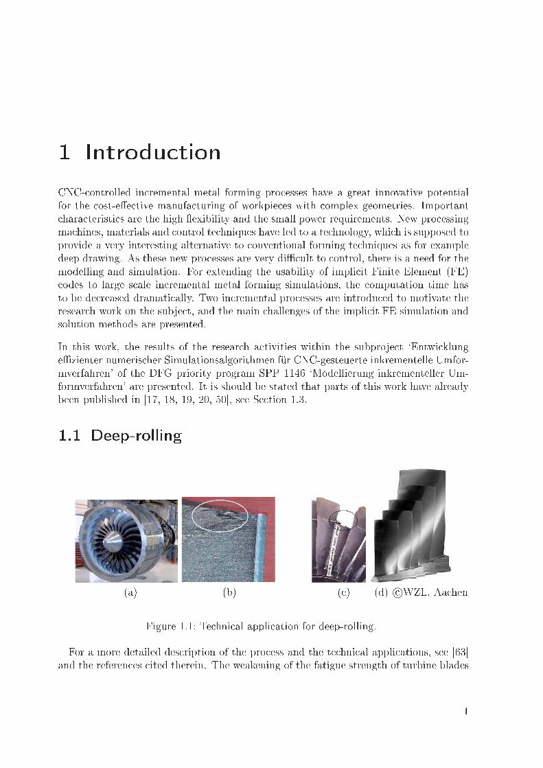
(a) (b) ( ) (d) ©WZL, Aa henFigure 1.1: Te hni al appli ation for deep-rolling.For a more detailed des ription of the pro ess and the te hni al appli ations, see [63and the referen es ited therein. The weakening of the fatigue strength of turbine blades1

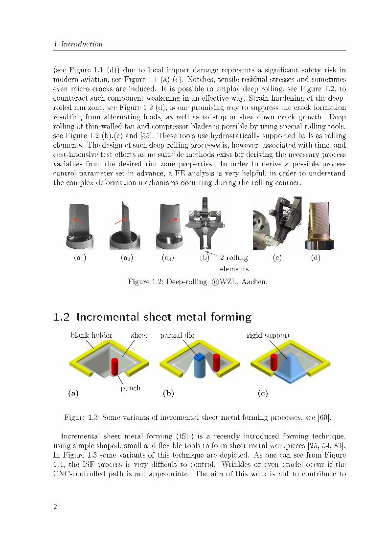
1 Introdu tion(see Figure 1.1 (d)) due to lo al impa t damage represents a signi ant safety risk inmodern aviation, see Figure 1.1 (a)-( ). Not hes, tensile residual stresses and sometimeseven mi ro ra ks are indu ed. It is possible to employ deep rolling, see Figure 1.2, to ountera t su h omponent weakening in an ee tive way. Strain hardening of the deep-rolled rim zone, see Figure 1.2 (d), is one promising way to suppress the ra k formationresulting from alternating loads, as well as to stop or slow down ra k growth. Deeprolling of thin-walled fan and ompressor blades is possible by using spe ial rolling tools,see Figure 1.2 (b),( ) and [55. These tools use hydrostati ally supported balls as rollingelements. The design of su h deep-rolling pro esses is, however, asso iated with time- and ost-intensive test eorts as no suitable methods exist for deriving the ne essary pro essvariables from the desired rim zone properties. In order to derive a possible pro ess ontrol parameter-set in advan e, a FE analysis is very helpful, in order to understandthe omplex deformation me hanisms o urring during the rolling onta t.(a1) (a2) (a3) (b) ( ) (d)PPi 2 rollingelementsFigure 1.2: Deep-rolling, ©WZL, Aa hen.1.2 In remental sheet metal forming

Vollpatrize

Umformkopf

Vollpatrizeblank holder sheet partial die rigid supportpun h(a) (b) ( )Figure 1.3: Some variants of in remental sheet metal forming pro esses, see [60.In remental sheet metal forming (ISF) is a re ently introdu ed forming te hnique,using simple shaped, small and exible tools to form sheet metal workpie es [25, 54, 83.In Figure 1.3 some variants of this te hnique are depi ted. As one an see from Figure1.4, the ISF pro ess is very di ult to ontrol. Wrinkles or even ra ks o ur if theCNC- ontrolled path is not appropriate. The aim of this work is not to ontribute to2

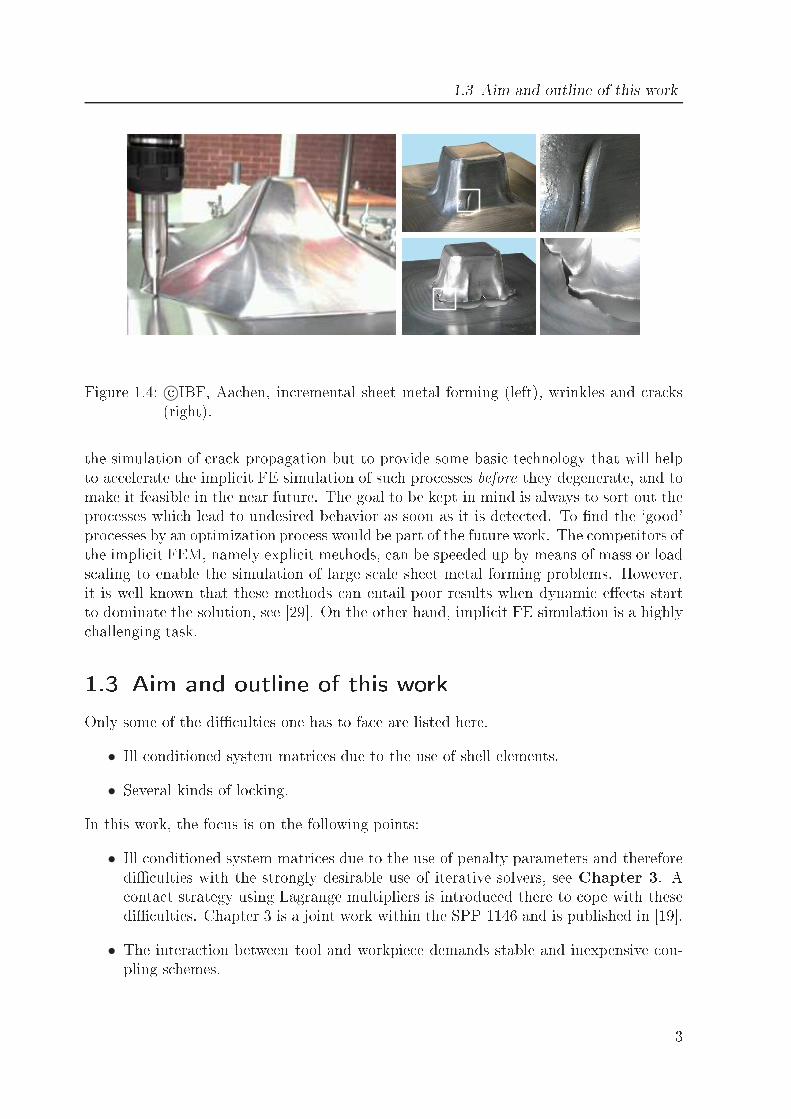
1.3 Aim and outline of this work

Figure 1.4: ©IBF, Aa hen, in remental sheet metal forming (left), wrinkles and ra ks(right).the simulation of ra k propagation but to provide some basi te hnology that will helpto a elerate the impli it FE simulation of su h pro esses before they degenerate, and tomake it feasible in the near future. The goal to be kept in mind is always to sort out thepro esses whi h lead to undesired behavior as soon as it is dete ted. To nd the `good'pro esses by an optimization pro ess would be part of the future work. The ompetitors ofthe impli it FEM, namely expli it methods, an be speeded up by means of mass or loads aling to enable the simulation of large s ale sheet metal forming problems. However,it is well known that these methods an entail poor results when dynami ee ts startto dominate the solution, see [29. On the other hand, impli it FE simulation is a highly hallenging task.1.3 Aim and outline of this workOnly some of the di ulties one has to fa e are listed here.• Ill onditioned system matri es due to the use of shell elements.• Several kinds of lo king.In this work, the fo us is on the following points:• Ill onditioned system matri es due to the use of penalty parameters and thereforedi ulties with the strongly desirable use of iterative solvers, see Chapter 3. A onta t strategy using Lagrange multipliers is introdu ed there to ope with thesedi ulties. Chapter 3 is a joint work within the SPP 1146 and is published in [19.• The intera tion between tool and workpie e demands stable and inexpensive ou-pling s hemes. 3

1 Introdu tion• The forming zone is small but very mobile. The pun h is tou hing almost everypoint of the workpie e surfa e at some time in the pro ess. Therefore the numberof degrees of freedom (dof) has to be very large in a non-adaptive omputation.Also the number of time steps is very large sin e the total duration of an in re-mental shaping pro edure is at least several minutes. The main idea to ta klethese problems is to use a `divide and onquer' approa h: A dynami overlappingdomain de omposition (ODDM) is employed by dis retizing the global workpie ewith a oarse mesh and the small forming zone with a relatively ne mesh, seeChapter 6. In Chapter 2 and Chapter 3, a short review of the lassi al FEsolution pro ess without any adaptive omputation is re alled. Parts of Chapter2 have been published in [17. The purpose of these two hapters is also to pro-vide denitions and notations whi h are needed in the des ription of the ouplingalgorithm. The two main aspe ts of this algorithm, the treatment of the materialnonlinearity and the treatment of the onta t are explained in Chapter 6 and rst onsiderations are made about the blo kwise (rst blo k: oarse system, se ondblo k: ne system) solution pro ess. The results of this hapter are published in[20. In Chapter 7, the solution pro ess is improved and put into the perspe tiveof lassi al inexa t Newton s hemes.• Sometimes ISF simulations are performed dynami ally and with an impli it timeintegration for two reasons:1. ISF an a tually be regarded as a dynami pro ess sin e elasti waves aretravelling through the material and dynami springba k (movement of theworkpie e due to a sudden load hange or after it is released from the lamping)o urs.2. It seems to be a reasonable hope that a omputation with a lumped mass ma-trix will improve the ondition number of the overall ee tive stiness matrix[84 and will help to over ome di ulties in the pre-bu kling phase.These two points are not ompletely within the s ope of this work, however energy onsistent time integration of the onta t problem is a prerequisite for these pointsand is treated in Chapter 4. For the energy onsistent treatment of plasti ity inthe regime of large deformations, pioneering work has been done, see for example[86 and the referen es therein.• First steps were taken for the dynami onta t analysis of thin walled stru tures,see Chapter 4 whi h is a result of a ooperation with Ramm/Hartmann [50.• Complex linearization problems arise due to1. displa ement based (Chapter 3) and velo ity based (Chapter 5, publishedin [18) onta t problems (boundary nonlinearity)2. the elastoplasti onstitutive law, Chapter 2 (material nonlinearity)3. large deformations, Chapter 8 (geometri nonlinearity)4

1.3 Aim and outline of this work• Finally, the a eleration of the omputation by using iterative solvers e ientlyespe ially in the framework of inexa t Newton methods is a topi of Chapter 3and Chapter 7.In Chapter 9, on luding remarks are made. One last word on the itations: Worksfrom several dis iplines of omputational me hani s and numeri al mathemati s are itedhere. Although all quoted works are important ontributions to these elds, the list israther fragmentary, and the author apologizes to those who had deserved to be quotedhere and are not.

5

2 Classi al 1-grid dis retization:Plasti ityA short review of the lassi al FEM solution pro ess of elastoplasti problems without anymesh-adaptivity is re alled in this hapter. Some basi on epts of metal plasti ity willbe onsidered and the need for onsistent linearization of the onstitutive relations. Inorder to keep the des ription of the oupling te hnique in Chapter 6 lear, a quite simplematerial model was used, namely elastoplasti ity for small deformations, see lassi altextbooks on omputational me hani s and plasti ity [10, 49, 97, 109 and the referen es ited therein.2.1 Introdu tionIn many large s ale forming simulation FE pa kages there is the problem that the mod-eling of elastoplasti ity is only validated well with examples like deep-drawing or otherexamples where the plasti strain, here in this work taken as the driving variable, isin reasing in every time step. In remental forming operations, make greater demandson the elastoplasti simulation be ause of the permanently hanging loading situation.In this hapter, the linearization of the onstitutive equations emphasized and not thelarge deformations. In Se tion 2.2 and Se tion 2.3, a simple plasti ity model the niteelement dis retization are detailed. In Se tion 2.4, a lassi al return mapping algorithmis dis ussed and the so alled onsistently linearized material tangent is derived. InSe tion 2.5, the tangent utting plane algorithm is dis ussed whi h is implemented inLARSTRAN/SHAPE [33, a FE pa kage dedi ated to metal forming simulations. Ina quite dierent dire tion goes the sequential quadrati programming (SQP) approa h.This is presented in Se tion 2.6. In Se tion 2.7 the dierent approa hes for the algorith-mi treatment of the onstitutive law are briey ompared. In Se tion 2.8 and in Se tion2.9, numeri al results and some rules for tensor al ulus are given.2.2 Governing equations and notationsIt is assumed here, that an additive de omposition of the linearized strain tensor ε ∈ Rd×d(d ∈ 2, 3 is the problem dimension) into an elasti part εe and a plasti part εp is valid.7

2 Classi al 1-grid dis retization: Plasti ityThe governing equations for the onstitutive law are the following:εe := ε− εp (2.1)σ = Celεe (2.2)εp = λ∂σΦ(σ, α) (2.3)α = λ (2.4)

λ ≥ 0, Φ(σ, α) ≤ 0 and λΦ(σ, α) = 0with σ ∈ Rd×d the a tual Cau hy stress, λ ∈ R the plasti onsisten y parameter.The 4th order tensor Cel(µL, λL) is the isotropi elasti material tensor with the Laméparameters (µL, λL) and Φ : Rd×d × R→ R is the yield fun tion dened byΦ(σ, α) = σ − Y (α) (2.5)By Y : R→ R, the fun tion of isotropi hardening with the hardening parameter α ∈ Ris denoted. The equivalent stress (·) : Rd×d → R an be dened by

σ :=

a0

√devσ : devσ von Mises

(

12

[

a|K1 +K2|M + a|K1 −K2|M + (2− a)|2K2|M])1/M Barlat/Lian, [7... ... (2.6)with

K1 :=1

2(σxx + hσyy), K2 :=

√

1

4(σxx − hσyy)2 + p2σ2

xyand a, h, p,M material parameters for the Barlat/Lian yield fun tion and with the di-mension dependent s aling fa tora0 :=

√

d

d− 1for the von Mises yield fun tion. The fun tion of isotropi hardening an be dened byY (α) :=

Y (0) +Kα linear isotropi ... ... (2.7)with K ∈ R+ the slope of the linear isotropi hardening urve. There is a vast literatureabout other possible yield fun tions, see [3.2.3 Global equilibrium iteration and Finite Elementdis retizationGiven a grid with N nodes and with FE ansatz fun tions φ1, . . . , φN , it is re alled brieyhow the global equilibrium iteration is set up: Sin e small deformations are assumed, all8

2.3 Global equilibrium iteration and Finite Element dis retizationintegrations an be arried out with respe t to the referen e onguration Ω. By H10 (Ω),the spa e of test fun tions with zero-Diri hlet boundary onditions 1 is denoted. Therelation σ = σ(u) is nonlinear and not even dierentiable in the strong sense. A losedform of the relation is not needed here. Usually, before spatial dis retization a timedis retization is performed. In addition to ommonly used Euler rst-order methods,whi h are used here, higher order methods with step size ontrol have gained in reasingattention in the last years, see for example [36 and the referen es therein. Throughoutthis hapter, the general trapezoidal rule (γ ∈ [0, 1])

zn+1 = zn + ∆t(γΦ(zn+1) + (1− γ)Φ(zn))is used with γ = 1 (ba kward, impli it Euler). The time step tn → tn+1 is onsidered andthe global equilibrium at the urrent time step tn+1 with the external for es f extn+1 a tingon the body is enfor ed. Strong emphasis should be pla ed on the fa t that the stress σndoes not only depend on the urrent displa ements un but also on the omplete path. Sothere is also a dependen e on un−1,un−2, . . . ,u1. The global equilibrium equation readsin weak form

f int(un+1,v) :=

∫

Ω

σn+1(un+1) : ε(v) =

∫

Ω

f extn+1 · v =: lext

n+1(v), v ∈ [H10 (Ω)]d (2.8)Dis retize un+1 by uh

n+1 and dene the ve tors F int(Un+1) and F ext as standard FEassemblies of f int and lext and the ve tor F (Un+1) asF (Un+1) := F int(Un+1)− F extA few remarks on the notation: The di tions F [i] and Fi mean the same, namely the

ith omponent of the ve tor F . Often FE fun tions, for example uh, are identied withtheir oe ient ve tor U , and sometimes the time index n is omitted. With this, theequilibrium equation (2.8) in the dis rete form is formulated now:F (Un+1) = 0 (2.9)After onsistent linearization [97, 99, one arrives at a global system of linear equationswith the tangential stiness K

(j)n+1 in the jth Newton step dened as

K(j)n+1[ik] :=

∂F (U(j)n+1)[i]

∂U (j)[k]=∂F int(U

(j)n+1)[i]

∂U (j)[k](2.10)1 onvenient abuse of notation in order to keep the notation simple in the ase when more than oneDiri hlet boundary is involved 9

2 Classi al 1-grid dis retization: Plasti ityThe orresponding derivative is determined as follows (sometimes the relation σ = σ(u)is not written expli itly):K

(j)ik =

∂F inti (U

(j)n+1)

∂U(j)k

=

∫

Ω

∂

∂U(j)k

σ(j)n+1 : ε(φi)

=

∫

Ω

ε(φk) : Cep,(j)n+1 : ε(φi) (2.11)In the last equality, the hain rule was used with the inner derivative ∂

∂Ukε(Un+1) = ε(φk)and the outer derivative, whi h shall be dened as the 4th order tensor

Cep,(j)n+1 :=

∂σ(j)n+1

∂ε(U(j)n+1)

(2.12)whi h is denoted as elastoplasti tangent. Finally, the zone of plasti deformation Ωp,n ⊂Ω at the time step tn is dened as the zone where new plasti deformation takes pla e:

Ωp,n := x ∈ Ω : εp(x, tn) 6= εp(x, tn−1) (2.13)This denition will be needed in the oupling algorithm.The following se tions are basi ally on erned with the elastoplasti tangent in Equation(2.12) and the fulllment of the yield ondition.Remark: The notation in (2.12) is a little bit sloppy: It turns out that F is only aLips hitz ontinuous fun tion. Thus, Cep,(j)n+1 annot be viewed as a unique total derivativebut it is one element of the generalized Ja obian as it is introdu ed by Clarke, see forexample [62.2.4 A Gauss point se tion: Radial Return for linearisotropi hardeningNow the radial return (RR) algorithm for linear isotropi hardening is des ribed. Thepurpose of this algorithm is to fulll the onstitutive Equations (2.1) - (2.4) at the end ofea h load step. One sees that within the framework of this stress integration algorithm, a onsistent material tangent an be readily obtained. Ex ept for minor te hni al details,the resulting algorithm is the same as do umented in, e.g., [97.Denitions The yield fun tion is now spe ied to a von-Mises type of yield fun tionwith linear isotropi hardening (the rst ase in (2.6) and in (2.7)). Some abbreviations10

2.4 A Gauss point se tion: Radial Return for linear isotropi hardeninghave to be made.λ := a2

0λ s aled plasti onsisten y parameter (2.14)s := dev(σ) deviatori stress

||σ|| :=√σ : σ Frobenius normBe ause of the stru ture of Φ, the ordinary dierential equation for the evolution of theplasti strain an be written expli itly in terms of the stress:

εp = λa0s

||s|| = λs

s(2.15)Here is s = a0

√dev s : dev s = a0||s|| a ording to Equation (2.6)1. In the followingalgorithm, the notations 1, I and

Idev := I− 1

d1⊗ 1are used for the se ond order identity tensor, the fourth order symmetri identity tensorand the fourth order deviatori tensor.Algorithm [ε

p,(j)n+1 ,σ

(j)n+1,C

ep,(j)n+1 , α

(j)n+1] = RADIAL_RETURN(ε(j−1)

n+1 , εpn, αn,Φ)1. Compute trial stress

κ := λL −2

dµL bulk modulus

en+1 := Idevε(j−1)n+1 deviatori strain

strn+1 := 2µL(en+1 − εp

n) trial deviatori stress2. Che k yield onditionΦtr

n+1 := strn+1 − Y (αn) evaluation of the yield fun tionIF Φtr

n+1 6 0 THEN:σ

(j)n+1 := κ tr(ε

(j−1)n+1 ) + str

n+1

εp,(j)n+1 := εp

n

Cep,(j)n+1 := Cel

α(j)n+1 := αnAND EXIT 11

2 Classi al 1-grid dis retization: Plasti ity3. Compute ow dire tion nn+1 and plasti onsisten y parameter λλ := root[g(λ) = 0] plasti onsisten y parameter, see Se tion 2.4.2

nn+1 :=1

||strn+1||

strn+1 ow dire tion

nn+1 := a−10 nn+1 s aled ow dire tion

α(j)n+1 := αn + λ ba kward Euler for (2.4) (2.16)4. Update plasti strain and stress a ording to (2.15)

εp,(j)n+1 := εp

n + λnn+1

σ(j)n+1 := κ tr(ε

(j−1)n+1 )1 + str

n+1 − 2µLλnn+1

= κ tr(ε(j−1)n+1 )1 + str

n+1 − 2µLa0λnn+1 (2.17)5. Compute the onsistent elastoplasti tangent module Cep,(j)n+1 a ording to Equation(2.18)2.4.1 Consistent elastoplasti tangent moduleFor the sake of brevity, the index for the Newton iteration (j) is omitted in the following.With (2.21) and some equations from tensor al ulus, see Se tion 2.9, the followingderivatives an be omputed:

∂εn+1(tr(εn+1)1) = 1⊗ 1

∂εn+1(λnn+1) = nn+1 ⊗∂λ

∂εn+1− λ∂nn+1

∂εn+1

∂λ

∂εn+1=

a−10

a−20 K + 2µL

strn+1

||strn+1||

:∂str

n+1

∂εn+1=

a−10

a−20 K + 2µL

2µL

strn+1

||strn+1||

= 2µLa−1

0

a−20 K + 2µL

nn+1Using the fa t that nn+1 is tra e-free:∂εn+1nn+1 =

∂nn+1

∂strn+1

∂strn+1

∂εn+1

=1

||strn+1||

(I− nn+1 ⊗ nn+1)∂str

n+1

∂εn+1

=1

||strn+1||

(I− nn+1 ⊗ nn+1)2µLIdev

=2µL

||strn+1||

(Idev − nn+1 ⊗ nn+1)12

2.4 A Gauss point se tion: Radial Return for linear isotropi hardeningWith this, one arrives at the desired tangent module:C

epn+1 =

∂σn+1

∂εn+1

= κ 1⊗ 1 + 2µL Idev − 2µL a0

[

nn+1 ⊗∂λ

∂εn+1

+ λ∂nn+1

∂εn+1

]

= Cel − 2µL a0 nn+1 ⊗2µL a

−10

a−20 K + 2µL

nn+1 − 2µL a02µLλ

||strn+1||

(Idev − nn+1 ⊗ nn+1)

= Cel −Cpn+1 (2.18)with the abbreviations

θ :=2µL

a−20 K + 2µL

− 2µL λ

strn+1

Cpn+1 := 2µL

2µL λ

strn+1

Idev − 2µLa20θ nn+1 ⊗ nn+1 (2.19)2.4.2 Plasti onsisten y parameterThe aim of this se tion is to ompute an expression for the plasti onsisten y parameter

λ. The deviatori part of Equation (2.17) is:sn+1 − str

n+1 + 2µLa0λ nn+1 = 0Multiplying this with n⊤n+1 and using that

nn+1 =strn+1

||strn+1||

=sn+1

||sn+1||one gets:g(λ) := ||sn+1|| − ||str

n+1||+ 2µLa0λ = 0 (2.20)Using that the yield ondition is fullled at tn+1 and with the aid of (2.16), one an ompute:g(λ) = a−1

0 Y (αn+1)− ||strn+1||+ 2µLa0λ

= a−10 Y (0) + a−1

0 Kαn+1 − ||strn+1||+ 2µLa0λ

= a−10 Y (0) + a−1

0 K(αn + λ)− ||strn+1||+ 2µLa0λThe onsisten y parameter λ an be written expli itly here as root of g.

λ =a−1

0 Y (0) + ||strn+1|| − a−1

0 Kαn

a−10 K + 2a0µL

(2.21)⇔ λ =

−Y (0)−Kαn + strn+1

a−20 K + 2µL

(2.22)Note that onsistent linearization of the RR algorithm is also straightforward in the ase of nonlinear isotropi and kinemati hardening, see [97, as long as the ontext ofJ2-plasti ity is not left. 13

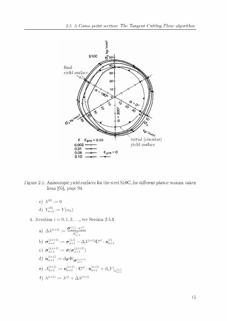
2 Classi al 1-grid dis retization: Plasti ity2.5 A Gauss point se tion: The Tangent CuttingPlane algorithmThe following algorithm is given in [3. It is based on works on tangent utting plane(TCP) algorithms like for example [98. A need for the tangent utting plane algorithmis given when1. anisotropi plasti ity o urs, e.g. the se ond ase of (2.6) applies. See the situationin Figure 2.1 (observe that the yield surfa e does not only hange the lo ationund size due to kinemati und isotropi hardening but also the shape due to theanisotropy), where lassi al return mapping algorithms do not apply any more2. and when the user annot or is not willing to provide twi e dierentiable yieldfun tions in order to make general return mapping algorithms ([97, Chapter 3)appli able.Unlike in Se tion 2.4, this Se tion is not restri ted to the ase of a von-Mises type yieldfun tion (2.6)1. Thus the deviatori parts of the stress and the strain tensors are not omputed in the TCP algorithm. Another dieren e to RR is that in this method a losed expression for λ like in Equation (2.21) annot be derived sin e the yield fun tionis supposed to be more general. Hen e, a lo al Newton iteration, see Se tion 2.5.1, mustbe performed to guarantee the fulllment of the yield ondition and the starting iterateσ

(j,0)n+1 takes the role of the trial stress.Algorithm [σ

(j)n+1, ε

p,(j)n+1 ,C

ep,(j)n+1 , α

(j)n+1] = CUTTING_PLANE(ε(j−1)

n+1 , εpn, αn,Φ)1. Trial values

σ(j,0)n+1 := Cel : (ε

(j−1)n+1 − εp

n)

εp,(j,0)n+1 := εp

n

α(j,0)n+1 := αn2. Che k yield onditionIF σ(j,0)

n+1 − Y (αn) 6 0 THENSET (•)(j)n+1 := (•)(j,0)

n+1 AND Cep,(j)n+1 := CelAND EXIT3. Initializationa) n

(0)n+1 := ∂σΦ|σ(j,0)

n+1∈ Rd×db) A(0)

n+1 := n(0)n+1 : Cel : n

(0)n+1 + ∂αΦ|

α(j,0)n+114

2.5 A Gauss point se tion: The Tangent Cutting Plane algorithm

@@

@I initial ( ir ular)yield surfa e

@@R

nalyield surfa e

Figure 2.1: Anisotropi yield surfa es for the steel S10C, for dierent plasti strains, takenfrom [65, page 94. ) λ(0) := 0d) Y (0)n+1 := Y (αn)4. Iteration i = 0, 1, 2, . . ., see Se tion 2.5.1a) ∆λ(i+1) :=

σ(j,i)n+1−Y

(i)n+1

A(i)n+1b) σ(j,i+1)

n+1 := σ(j,i)n+1 −∆λ(i+1)Cel : n

(i)n+1 ) σ(j,i+1)

n+1 := σ(σ(j,i+1)n+1 )d) n

(i+1)n+1 := ∂σΦ|σ(j,i+1)

n+1e) A(i+1)n+1 := n

(i+1)n+1 : Cel : n

(i+1)n+1 + ∂αY |α(j,i)

n+1f) λ(i+1) := λ(i) + ∆λ(i+1) 15

2 Classi al 1-grid dis retization: Plasti ityg) α(j,i+1)n+1 := α

(j,i)n+1 + ∆λ(i+1)h) εp,(j,i+1)

n+1 := εp,(j,i)n+1 + ∆λ(i+1)n

(i+1)n+1i) Y (i+1)

n+1 := Y (α(j,i+1)n+1 )j) IF σ(j,i+1)

n+1 − Y (i+1)n+1 < TOLΦ THENINNER ITERATION FINISHED, GOTO 5ELSE i = i+ 1 GOTO 4ENDIF5. Elastoplasti module C

ep,(j)n+1 := Cel − 1

An+1(Cel : nn+1)⊗ (Cel : nn+1)Details about the ba kground an be found in [3. Only a few points are dis ussed here,espe ially the fulllment of the yield ondition and the elastoplasti tangent whi h arethe two most important dieren es to the RR algorithm in Se tion (2.4).2.5.1 Fulllment of the yield onditionAn equation for the plasti onsisten y parameter has to be developed, su h that theyield ondition is fullled in the urrent Newton step.

Φ(j)n+1(λ) = Φ(σ

(j)n+1(λ), α

(j)n+1(λ))

!= 0 (2.23)From this and Equations (2.4), (2.5) follows:

Φ(j)n+1 = σ

(j)n+1(λ)− Y (α

(j)n+1(λ))

∂λΦ(j)n+1 = ∂σΦ

(j)n+1 : ∂λσ

(j)n+1 − ∂αY

(j)n+1 ∂λα

(j)n+1

= −∂σΦ(j)n+1 : Cel

n+1 : ∂σΦ(j)n+1 − ∂αY

(j)n+1 (2.24)The last equation is obtained with the aid of

εp,(j)n+1 − εp

n = λ ∂σΦ(j)n+1 (ba kward Euler s heme for Equation (2.1))

σ(j)n+1 − σn = Cel : [εn+1 − εp,(j)

n+1 − εn + εpn]

= Cel : [εn+1 − εn − λ ∂σΦ(j)n+1]

∂λσ(j)n+1 = −Cel : ∂σΦ

(j)n+1Note that the total strain εn+1 does not depend on λ. So, with the aid of (2.24), theNewton s heme for nding the root of Φ reads like this:

∂λΦ(j)n+1|λ(i) ∆λ(i+1) = −Φ

(j)n+1(λ

(i))with∆λ(i+1) =

Φ(j)n+1(λ

(i))[

∂σΦ(j)n+1 : Cel : ∂σΦ

(j)n+1 + ∂αY

(j)n+1

]

λ(i)16

2.6 A Gauss point se tion: Sequential quadrati programming2.5.2 Dis ussionOne of the problems arising here is that the yield ondition is fullled but Cep,(j)n+1 in Point5 of Algorithm CUTTING_PLANE is not the onsistent material tangent. Indeed one ansee that (2.12) is not fullled by the tangent utting plane algorithm presented here. Infa t it is derived from the time- ontinuous tangent

Cep =∂σ

∂εsee for example [3. This is done be ause it is very di ult to obtain a losed expression forthe nal σ(j)n+1, see line 4b, sin e there is no expli it expression for a root λ of the nonlinearEquation (2.23). As it is shown in the results in Se tion 2.8, no good onvergen e isa hievable using this tangent, even in the ase of the simple von Mises yield fun tion.2.6 A Gauss point se tion: Sequential quadrati programmingIn this se tion, another method for solving the onstrained optimization problem is given,namely sequential quadrati programming (SQP). In [105 the method is des ribed andapplied to perfe t plasti ity (no hardening, Φ = Φ(σ)). The basi idea is to use the fa tthat it is not ne essary to fulll the yield ondition in ea h semismooth Newton step.The Newton iteration is repla ed by a sequen e of quadrati minimization problems withlinearized onstraints (`linearized proje tion step'). The advantage of the SQP method isthe large exibility whi h allows to enhan e it to more general plasti ity models, where thegeneralization of the Radial Return algorithm is not straightforward. Another importantpoint is the mesh independent onvergen e of the SQP loop.2.6.1 DenitionsSome denitions have to be made: Let K be the set of admissible stresses

K := τ ∈ Sd×d : Φ(τ ) 6 0Let Sd×d denote the subset of symmetri matri es in Rd×d. Some variables for the lin-earized proje tion step j, namely the linearized ow rule Φ

(j)n+1, the quadrati dual en-ergy fun tional E (j)

n+1, the elastoplasti module Csqp,(j)n+1 , the half-spa e K

(j)n+1 of admissiblestresses with respe t to Φ

(j)n+1, the inner produ t e(j)n+1(·, ·) and the asso iated energy E(j)

n+117

2 Classi al 1-grid dis retization: Plasti ityare dened byΦ

(j)n+1(σ) := Φ(σ

(j−1)n+1 ) + ∂σΦ|σ(j−1)

n+1: (σ − σ(j−1)

n+1 ) (2.25)E (j)

n+1(σ) :=

∫

Ω

E(j)n+1

(

σ −Csqp,(j)n+1 : (εp

n + λ(j−1)∂σσΦ|σ(j−1)n+1

: σ(j−1)n+1 )

) (2.26)C

sqp,(j)n+1 := (I + λ(j−1)Cel ∂σσΦ|σ(j−1)

n+1)−1 Cel (2.27)

K(j)n+1 := τ ∈ S

d×d : Φ(j)n+1(τ ) 6 0 (2.28)

e(j)n+1(σ, τ ) := σ : (C

sqp,(j)n+1 )−1 : τ (2.29)

E(j)n+1(σ) :=

1

2σ : (C

sqp,(j)n+1 )−1 : σ (2.30)The trial stress θ(j)

n+1 is dened by:θ

(j)n+1(u) := C

sqp,(j)n+1 :

(

ε(u)− εpn + λ(j−1)∂σσΦ|σ(j−1)

n+1: σ

(j−1)n+1

) (2.31)2.6.2 Derivation of the SQP stepStarting point of the SQP step is the original system ontaining ow rule, omplementary onditions and equilibrium whi h is to be solved at the end of the load step:σn+1 −Cel :

(

ε(un+1)− εpn + λ∂σΦ|σn+1

)

= 0 (2.32)Φ(σn+1) 6 0, λΦ(σn+1) = 0, λ > 0 (2.33)∫

Ω

σn+1 : ε(v) = lextn+1(v), v ∈ [H1

0 (Ω)]d (2.34)Linearizing Equation (2.32) with respe t to (σn+1, λ,un+1), using the denitions (2.25)and (2.31) and using the equality∂σΦ|σ(j−1)

n+1= ∂σΦ

(j)n+1|σ(j)

n+1(Φ(j)n+1 is linear), one arrives after some algebrai manipulations at the result whi h willbe dis ussed in Se tion 2.6.3. Equation (2.33) and (2.34) are reformulated with thelinearized ow fun tion and the linearized material response, respe tively.2.6.3 The SQP step and the algorithmSo in ea h SQP step, the linearized ow rule and the linearized omplementary onditions

σ(j)n+1 − θ(j)

n+1 − λ(j)Csqp,(j)n+1 : ∂σΦ

(j)n+1|σ(j)

n+1= 0 (2.35)

Φ(j)n+1 6 0, λ(j)Φ

(j)n+1 = 0, λ(j) > 0 (2.36)18

2.6 A Gauss point se tion: Sequential quadrati programmingare solved at ea h integration point for (σ(j)n+1, λ

(j)) and this linearized material responseis inserted into the equilibrium equation:∫

Ω

σ(j)n+1 : ε(v) = lext

n+1(v), v ∈ [H10 (Ω)]d (2.37)The System (2.35)-(2.37) represents indeed a SQP step as it is equivalent to:Find a minimizer σ(j)

n+1 of E (j)n+1(·) subje t to the linear onstraints σ ∈ K

(j)n+1 and theequilibrium equation.In ontrary to σ ∈ K, the onstraint σ ∈ K

(j)n+1 is indeed linear sin e K

(j)n+1 is a half-spa e.Lemma 7 in [105 states that a unique solution σ(j)

n+1 of this problem exists sin e E (j)n+1(·)is uniformly onvex. So (without giving a formal proof) mesh-independent onvergen e an be expe ted.The nonlinear problem (2.37) is to be solved with an inner Newton iteration. Fortu-nately, the appli ation of an inexa t method is possible: It is not ne essary to iterate theinner Newton loop until onvergen e in ea h SQP step. Further inexa t methods willbe presented in the following hapters. SQP would insofar t very well to the divide-and- onquer approa h of this work: The di ulties of fullling the yield ondition andthe equilibrium ondition are separated in su h a way that omputational ost an beredu ed.A onsistent tangent module has to be omputed. For this purpose, problem (2.37) isslightly reformulated with the aid of Lemma 1 in [105, whi h states that the solution

σ(j)n+1 of [(2.35),(2.36) is uniquely determined as

σ(j)n+1 = Π

(j)n+1(θ

(j)n+1) (2.38)where Π

(j)n+1 is the e(j)n+1(·, ·)-orthogonal proje tion onto the half-spa e K

(j)n+1. Then

fint,(j)n+1 (u,v) :=

∫

Ω

Π(j)n+1(θ

(j)n+1(u)) : ε(v)− lext

n+1(v)!= 0 (2.39)is equivalent to (2.37). By deriving ∂uf int,(j)

n+1 |u(j,i)n+1

, one gets the onsistent tangent moduleC

ep,(j,i)n+1 :=

∂Π(j)n+1

∂θ|θ

(j)

n+1(u(j,i)n+1)

Csqp,(j)n+1 (2.40)in the inner Newton step i. Now, the solution algorithm is given; note that j is in this ontext the index of the SQP iteration and i index of the inner Newton iteration.Algorithm [σn+1, ε

pn+1] = SQP(εp

n,Φ, λn,σn,un)1. Init. u(0)n+1 := un,σ

(0)n+1 := σn, λ

(0)n+1 := λn and j := 1 19

2 Classi al 1-grid dis retization: Plasti ity2. Init. u(j,0)n+1 := u

(j−1)n+1 and i := 13. Compute the trial stress

θ(j)n+1(u

(j,i−1)n+1 )a ording to Equation (2.31) and the linearized proje tion

σ(j,i−1)n+1 = Π

(j)n+1(θ

(j)n+1(u

(j,i−1)n+1 ))a ording to Equation (2.38) for the Newton residual of the nonlinear problem(2.39).4. If |f int,(j,i−1)

n+1 | is not small enough then goto step 5 else goto step 6.5. Compute Cep,(j,i)n+1 a ording to (2.40) and ompute ∆u

(j,i)n+1 as Newton step in thesolution of the nonlinear problem (2.39) with the residual, omputed in step (3).Update

u(j,i)n+1 := u

(j,i−1)n+1 + ∆u

(j,i)n+1set i := i+ 1 and goto step 3.6. Set u(j)

n+1 := u(j,i)n+1,σ

(j)n+1 := σ

(j,i)n+1 and λ(j) := λ(j,i)7. If

||σ(j)n+1 −Cel :

(

ε(u(j)n+1)− εp

n + λ(j)∂σΦ|σ(j)n+1

)

||whi h is the residual of Equation (2.32), is not small enough, set j := j + 1 andgoto step 3 else goto step 88. Set un+1 := u(j)n+1,σn+1 := σ

(j)n+1, λ := λ(j) and εp

n+1 := εpn + λ∂σΦ|σn+1 and exit.2.7 Comparison of the Gauss point algorithmsThe dierent algorithms for stress integration are ompared in some headwords. Thegeneralized proje tion method will be explained in the ontext of nite plasti ity. Thereare more possibilities to solve the onstrained optimization problem whi h are not listedhere, for example the interior point method whi h has been applied to plasti ity in [69.Consistently linearized RR, see Se tion 2.4

• For ertain types of yield fun tions easy to linearize onsistently.• Di ult to adapt to general yield fun tions. In the general ase, onsistent lin-earization di ult.20

2.8 Numeri al resultsTCP, see Se tion 2.5• Appli able to many kinds of ow laws, in luding anisotropi plasti ity.• Consistent linearization very di ult.SQP, see Se tion 2.6• The fa t that the yield ondition does not need to be fullled in ea h Newton step an be used to save omputation time.• Outer SQP loop and inner Newton loop.• Appli able to many kinds of ow laws, in luding anisotropi plasti ity sin e in ea hSQP step a ba k proje tion onto a simple half-spa e is performed.• Mesh independent and good onvergen e of the outer SQP loop.Generalized proje tion, see Se tion 8.5• Appli able to many kinds of ow laws, in luding anisotropi plasti ity.• Consistent linearization easy.• Fulllment of the yield ondition more ostly sin e a Newton iteration has to beperformed to ompute the stresses and the plasti data.2.8 Numeri al results

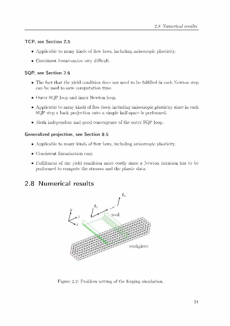
tool

workpie ey

z

x

t1

tn

Figure 2.2: Problem setting of the forging simulation. 21

2 Classi al 1-grid dis retization: Plasti ityIn this se tion, TCP and RR are ompared by means of an elastoplasti forging-likesimulation, depi ted in Figure 2.2. The assumptions are J2 plasti ity, linear isotropi hardening and small deformations. So, ea h FE element with TCP, whi h is formulatedfor the more general ase of anisotropi plasti ity, is expe ted to behave like an elementwith the onsistently formulated RR algorithm. Results for (tn = tool feed in step n)t1,...,5 =

[

0−0.05

0

]

, t6,...,50 =[

00

0.1

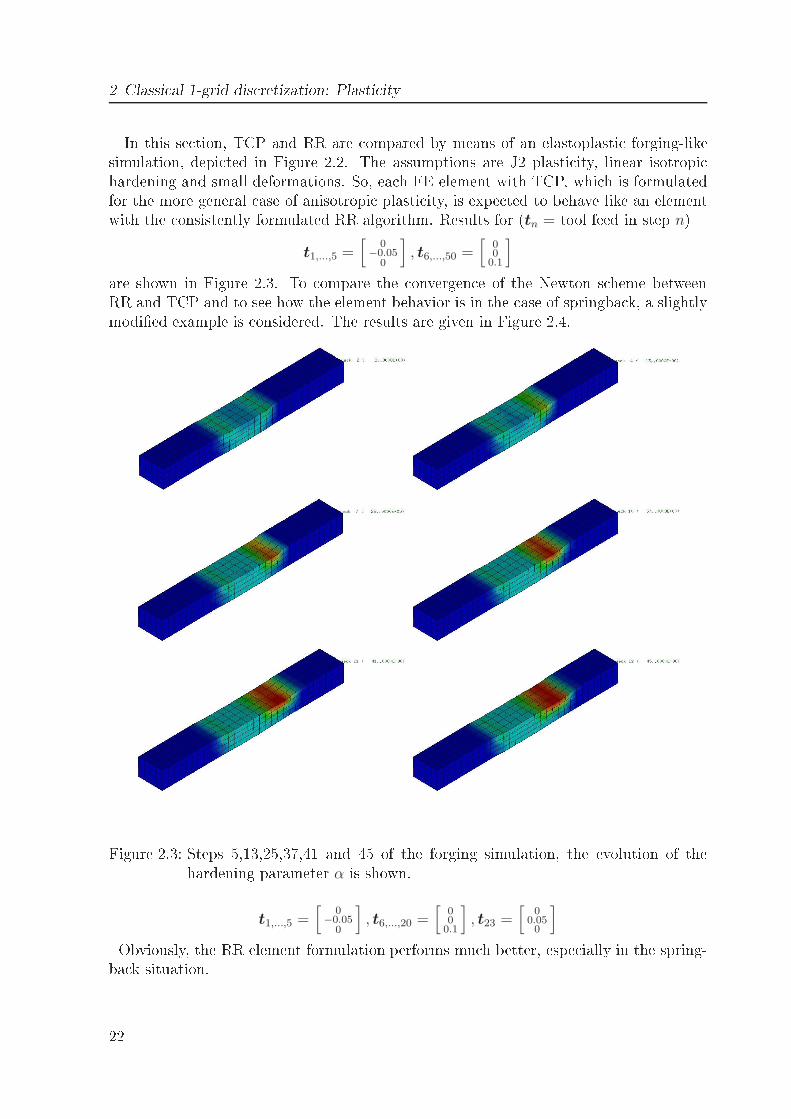
]are shown in Figure 2.3. To ompare the onvergen e of the Newton s heme betweenRR and TCP and to see how the element behavior is in the ase of springba k, a slightlymodied example is onsidered. The results are given in Figure 2.4.

Figure 2.3: Steps 5,13,25,37,41 and 45 of the forging simulation, the evolution of thehardening parameter α is shown.t1,...,5 =

[

0−0.05

0

]

, t6,...,20 =[

00

0.1

]

, t23 =[

00.050

]Obviously, the RR element formulation performs mu h better, espe ially in the spring-ba k situation.22

2.9 Some tensor al ulus0 10 20 30 40

10−15

10−10

10−5

100

iteration

New

ton−

erro

r (d

ispl

c)

Step 1, representative

RRTCP

0 2 4 6 8 10 1210

−8

10−6

10−4

10−2

100

iteration

New

ton−

erro

r (d

ispl

c)

Step 11, best performance of TCP

RRTCP

0 2 4 6 810

−15

10−10

10−5

100

105

1010

iteration

New

ton−

erro

r (d

ispl

c)

Step 23, springback, divergence of TCP

RRTCP

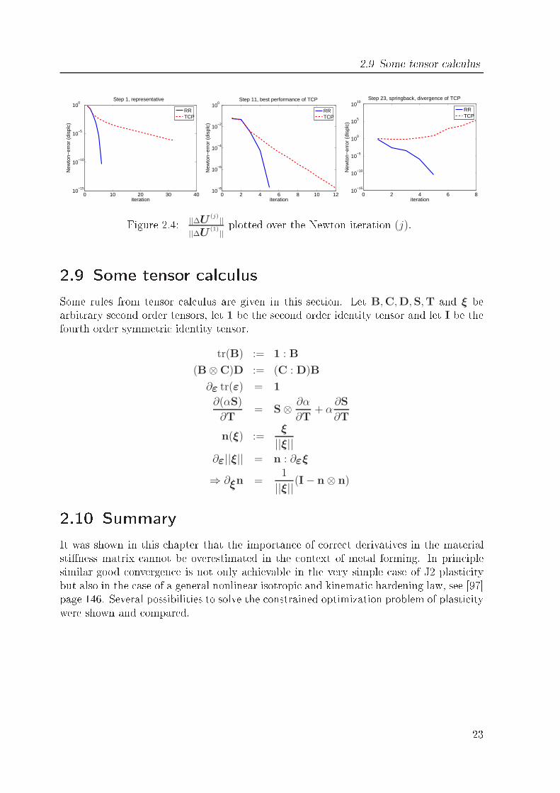
Figure 2.4: ||∆U(j)

||

||∆U(1)

||plotted over the Newton iteration (j).2.9 Some tensor al ulusSome rules from tensor al ulus are given in this se tion. Let B,C,D,S,T and ξ bearbitrary se ond order tensors, let 1 be the se ond order identity tensor and let I be thefourth order symmetri identity tensor.

tr(B) := 1 : B

(B⊗C)D := (C : D)B

∂ε tr(ε) = 1

∂(αS)

∂T= S⊗ ∂α

∂T+ α

∂S

∂T

n(ξ) :=ξ

||ξ||∂ε||ξ|| = n : ∂εξ

⇒ ∂ξn =1

||ξ||(I− n⊗ n)2.10 SummaryIt was shown in this hapter that the importan e of orre t derivatives in the materialstiness matrix annot be overestimated in the ontext of metal forming. In prin iplesimilar good onvergen e is not only a hievable in the very simple ase of J2 plasti itybut also in the ase of a general nonlinear isotropi and kinemati hardening law, see [97page 146. Several possibilities to solve the onstrained optimization problem of plasti itywere shown and ompared.23

3 Classi al 1-grid dis retization:Conta tThe intera tion between tool and workpie e is modelled as one-body onta t problemwith a rigid obsta le. Fri tion is negle ted throughout this work but Tres a and Coulombfri tion an be in orporated in any of the algorithms presented here [56. For extendingthe usability of impli it FE odes for large s ale forming simulations, the omputationtime has to be de reased dramati ally. In prin iple, this an be a hieved by using iterativesolvers. In order to fa ilitate the use of this kind of solvers, one needs a onta t algorithmwhi h does not deteriorate the ondition number of the system matrix and thereforedoes not slow down the onvergen e of iterative solvers like penalty formulations do.Additionally, an algorithm is desirable whi h does not blow up the size of the systemmatrix like methods using standard Lagrange multipliers. The work detailed in [19shows that a onta t algorithm based on a primal-dual a tive set strategy (pdASeS)provides these advantages and is therefore highly e ient with respe t to omputationtime in ombination with fast iterative solvers, espe ially algebrai multigrid methods.3.1 Conta t algorithms in the literatureE ient onta t algorithms have been developed in re ent years, see [75, 92, 110, 111, 112and the referen es therein. For more omplex onta t problems where the onta t area isnot known in advan e, a tive set strategies are well established nowadays. Four importantvariants of them are listed with their advantages (+) and disadvantages (−), see forexample Willner [106 and the referen es therein.Penalty formulation+ Pure displa ement based formulation, no hange in the system size.− For small values of the penalty parameter, the penetration is quite large.− For large values of the penalty parameter, the ondition number of the systemmatrix is deteriorated.Standard Lagrange multipliers+ Exa t fulllment of the orresponding dis rete non-penetration ondition.+ No deterioration of the ondition number of the stiness matrix. 25

3 Classi al 1-grid dis retization: Conta t− The multipliers are additional unknowns, the size of the system matrix in reases.− Only global elimination of the LM is possible leading to dense matri es.Perturbed Lagrangian formulation+ Very sti onstitutive laws pose no numeri al problems.+ No deterioration of the ondition number of the stiness matrix.− Mixed method, the size of the system matrix in reases.− Only global elimination of the LM is possible leading to dense matri es.Augmented Lagrangian formulation+ Nearly exa t fulllment of the non-penetration ondition with low penalties.+ No hange in the system size.+ No deterioration of the ondition number of the stiness matrix.− Higher numeri al osts due to extra augmentation loop.The algorithm, proposed here, whi h goes ba k to [2, 53, unies the advantages ofLagrange multipliers and the penalty method:Dual Lagrange multipliers+ No hange in the system size due to the use of dual Lagrange multipliers, whi hmakes the method very useful even for large ommer ial FE pa kages.+ Exa t fulllment of the geometri onstraints of the tool in a weak integral sense.+ No deterioration of the ondition number of the stiness matrix.There exists in the literature a large number of alternative methods su h as e.g. FETItype algorithms [34 and monotone methods [67, 70. In this work, the omparisonbetween the primal-dual a tive set strategy and the penalty method is emphasized, sin eone an see from the survey given above that the problems of the penalty formulationare somehow preserved in the other algorithms and just assume a dierent shape.26

3.2 The primal dual a tive set strategy with dual Lagrange multipliers3.2 The primal dual a tive set strategy with dualLagrange multipliersIn the following, the primal-dual a tive set strategy will be sometimes referred to as a tiveset strategy, keeping in mind that there are dierent kinds of a tive set strategies givenin the literature. It turns out that this strategy is very attra tive for the use in metalforming, espe ially in ombination with iterative solvers, as their onvergen e behaviorstrongly depends on the ondition number of the system matrix. Due to steady in reasein the problem size and the need for a robust, highly a urate and s alable solutionmethod, algebrai multigrid methods [31, 102 are the main fo us of this investigation.In [19, the a tive set strategy was adapted for nonlinear material behavior and somedetails were given about the implementation in LARSTRAN. It will be shown that in ombination with the a tive set strategy, the well-known good omplexity of multigridmethods an be a hieved. By using algebrai multigrid, problem dependen y an beover ome su h that the used solver provides a bla k-box hara ter. It will be shown thatthe Newton and the solver loop of the algebrai multigrid method an be merged. Thisinexa t strategy provides a further de rease in omputation time.To handle the nonlinearity of the KarushKuhnTu ker onta t onditions, a primal-dual a tive set strategy based on dual Lagrange multipliers [57, 108 is applied. This anbe interpreted as a Newton method [2, 53. In ontrast to the ommonly used penaltymethod [61, the a tive set strategy allows to adjust the geometri onstraints of the toolexa tly in a weak integral sense. This point will be explained in more detail in Chapter4. The onta t stress an be easily re overed from the displa ements in a variationally onsistent way and does not depend on a tuning parameter.3.2.1 Basi ideaJust to give a rst impression, a simple re tangular workpie e is onsidered whi h isindented by a rigid, hemispheri al pun h, see Figure 3.1a. By S the set of potential onta t nodes is denoted, see Figure 3.1a. Here, j is the iteration index for the a tive setloop. Let Aj ⊂ S be the a tive set, for whi h the body is in onta t with the obsta le.The omplementary set Ij := S − Aj is alled the ina tive set. The following simpletest example shows how the sets Ij+1 and Aj+1 are orre tly determined. The followingsituation is assumed, see Figure 3.1b, in the j-th step: Nodes 1,2 are a tive, nodes3,4 are ina tive. The tool geometry is then adjusted to the a tive nodes, no matter ifthe a tive set is already orre t or not, see Figure 3.1 . Now the nodal for es and thedete ted penetration are used to update the a tive and ina tive node sets:Aj+1 := p ∈ Ij : p penetrates ∪ p ∈ Aj : p under ompressionIj+1 := p ∈ Ij : no penetration ∪ p ∈ Aj : p under tensionThen the restri tions from the tool geometry are again adjusted to the orre t a tivenodes and the ina tive nodes are released, see Figure 3.1d. The step from ( ) to (d) is27

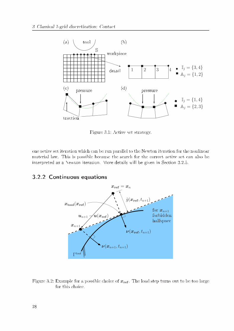
3 Classi al 1-grid dis retization: Conta t

tool workpie edetailS

1

PPPPPPPPPq2 3 4

Aj = 1, 2Ij = 3, 4

Aj = 2, 3Ij = 1, 4

?

pressure6tra tion ? ?

pressure(a) (b)( ) (d)

Figure 3.1: A tive set strategy.one a tive set iteration whi h an be run parallel to the Newton iteration for the nonlinearmaterial law. This is possible be ause the sear h for the orre t a tive set an also beinterpreted as a Newton iteration. More details will be given in Se tion 3.2.5.3.2.2 Continuous equations

xn+1

g(xref , tn+1)

xref = xn

xtool(xref )

ν(xref , tn+1)

ν(xn+1, tn+1)

Γtool

un+1 − u(xref )for xn+1forbiddenhalfspa e

Figure 3.2: Example for a possible hoi e of xref . The load step turns out to be too largefor this hoi e.28

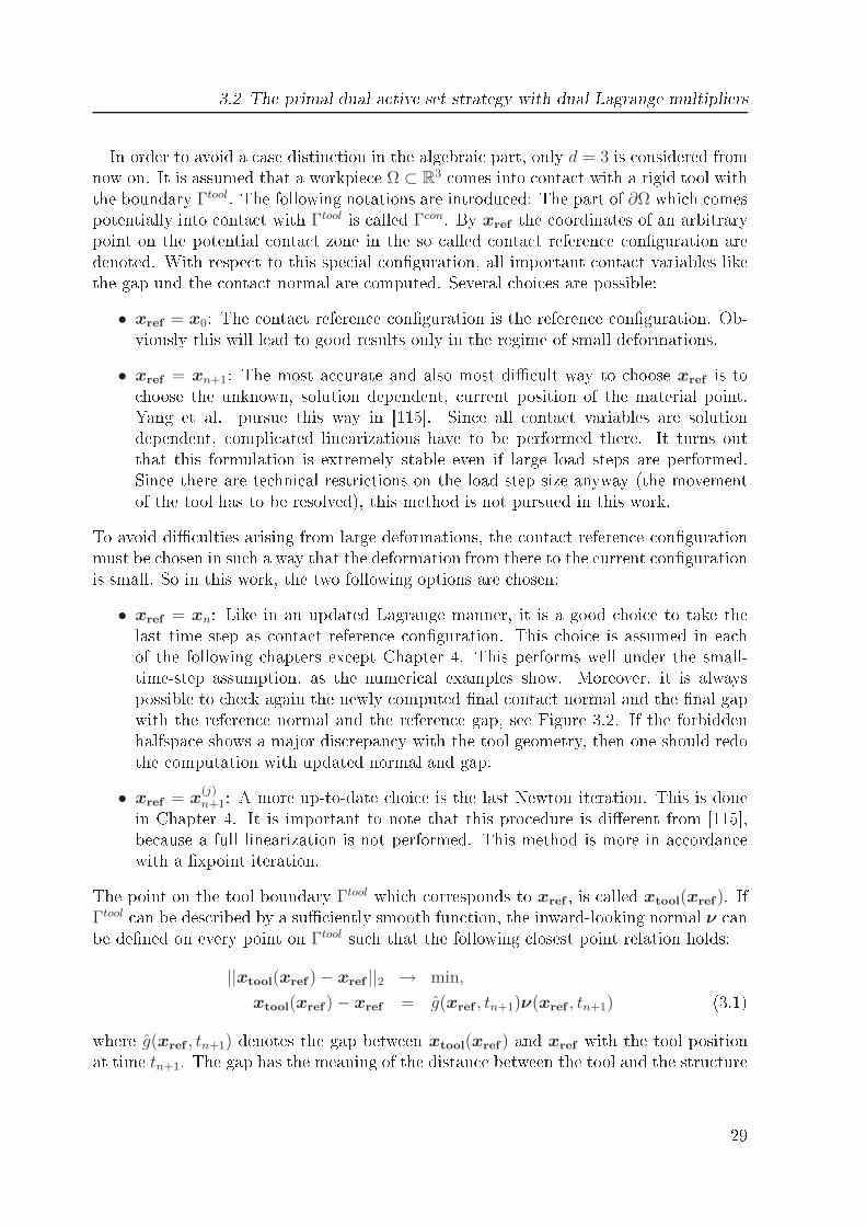
3.2 The primal dual a tive set strategy with dual Lagrange multipliersIn order to avoid a ase distin tion in the algebrai part, only d = 3 is onsidered fromnow on. It is assumed that a workpie e Ω ⊂ R3 omes into onta t with a rigid tool withthe boundary Γtool. The following notations are introdu ed: The part of ∂Ω whi h omespotentially into onta t with Γtool is alled Γcon. By xref the oordinates of an arbitrarypoint on the potential onta t zone in the so alled onta t referen e onguration aredenoted. With respe t to this spe ial onguration, all important onta t variables likethe gap und the onta t normal are omputed. Several hoi es are possible:• xref = x0: The onta t referen e onguration is the referen e onguration. Ob-viously this will lead to good results only in the regime of small deformations.• xref = xn+1: The most a urate and also most di ult way to hoose xref is to hoose the unknown, solution dependent, urrent position of the material point.Yang et al. pursue this way in [115. Sin e all onta t variables are solutiondependent, ompli ated linearizations have to be performed there. It turns outthat this formulation is extremely stable even if large load steps are performed.Sin e there are te hni al restri tions on the load step size anyway (the movementof the tool has to be resolved), this method is not pursued in this work.To avoid di ulties arising from large deformations, the onta t referen e ongurationmust be hosen in su h a way that the deformation from there to the urrent ongurationis small. So in this work, the two following options are hosen:• xref = xn: Like in an updated Lagrange manner, it is a good hoi e to take thelast time step as onta t referen e onguration. This hoi e is assumed in ea hof the following hapters ex ept Chapter 4. This performs well under the small-time-step assumption, as the numeri al examples show. Moreover, it is alwayspossible to he k again the newly omputed nal onta t normal and the nal gapwith the referen e normal and the referen e gap, see Figure 3.2. If the forbiddenhalfspa e shows a major dis repan y with the tool geometry, then one should redothe omputation with updated normal and gap.• xref = x

(j)n+1: A more up-to-date hoi e is the last Newton iteration. This is donein Chapter 4. It is important to note that this pro edure is dierent from [115,be ause a full linearization is not performed. This method is more in a ordan ewith a xpoint iteration.The point on the tool boundary Γtool whi h orresponds to xref , is alled xtool(xref ). If

Γtool an be des ribed by a su iently smooth fun tion, the inward-looking normal ν anbe dened on every point on Γtool su h that the following losest point relation holds:||xtool(xref )− xref ||2 → min,

xtool(xref )− xref = g(xref , tn+1)ν(xref , tn+1) (3.1)where g(xref , tn+1) denotes the gap between xtool(xref ) and xref with the tool positionat time tn+1. The gap has the meaning of the distan e between the tool and the stru ture29

3 Classi al 1-grid dis retization: Conta tin the onta t referen e onguration. The sign of this gap fun tion will dene whethera material point on the potential onta t zone will ome into onta t with the rigidobsta le or not. A positive value of g(x, t) indi ates that there is no onta t, whereas anegative value des ribes an interpenetration, whi h is prohibited. In the following, it willbe always written ν instead of ν(xref , tn+1) and g instead of g(xref , tn+1), and it will beassumed that the relation (3.1) holds. By u, the unknown displa ements xn+1 − x0 aredenoted, and by u(xref) the known displa ements xref − x0. Finally, the s alar valuednormal part σν(u) of the stresses on Γcon and the tangential stress ve tor στ (u) ∈ Rdare dened byσν(u) := (σ (u)ν) · ν, στ (u) := σ (u)ν − σν(u)ν (3.2)The well known onta t onditions for all xref in the potential onta t zone Γcon aregiven by (the time index n is omitted in this subse tion):

(u− u(xref )) · ν − g ≤ 0

σν(u) ≤ 0

σν(u) ((u− u(xref )) · ν − g) = 0

στ (u) = 0Hiding all the known information ing := g + u(xref ) · νthe onta t onditions an be written as

u · ν − g ≤ 0 (3.3)σν(u) ≤ 0 (3.4)

σν(u) (u · ν − g) = 0 (3.5)στ (u) = 0 (3.6)The onditions (3.3)-(3.6) an be interpreted in the following way:(3.3) means that no penetration is allowed.(3.4) allows only ompression but no tension, sin e there is no adhesion.(3.5) is the omplementary ondition that means that either non-zero onta t stressesare present and the gap is zero or the gap is non-zero and there are no onta tstresses.(3.6) nally means that the stress in tangential dire tion is zero, sin e there is no fri tion.The equilibrium is given by (for simpli ity volume for es and other external for es areassumed to be zero ex ept from the onta t for es): Find u ∈ [H1

0 (Ω)]3 su h thatf int(u,v) +

∫

Γcon

λ · v != 0 (3.7)30

3.2 The primal dual a tive set strategy with dual Lagrange multipliersfor arbitrary test fun tions v ∈ [H10 (Ω)]3 and with the internal for es f int dependingnonlinearly on u. The Lagrange multiplier λ := −σ(u)ν is exa tly the onta t stress,whi h is ne essary to adjust the onta t displa ements on the onta t boundary Γcon. Itis introdu ed as additional unknown to fulll the onta t onditions.3.2.3 A tive Set Strategy and Algebrai Multigrid MethodsLater in this hapter, the task will be to solve the linearized equation system (3.24).Multigrid methods have proven to be highly e ient for problems arising from niteelement dis retizations of partial dierential equations, see e.g. [48 and espe ially for onta t problems, see Kornhuber and Krause [68, 70. Due to the fa t that lo ally renedmeshes are widely used throughout engineering pra ti e for su h kind of problems, ahierar hi al grid stru ture might be very di ult to a hieve on large unstru tured grids.For that reason the fo us is on algebrai multigrid methods. They preserve the mainmultigrid properties but require only the system matrix of the (ne) omputational gridas input and thus appear to be very attra tive.Algebrai multigrid, rst introdu ed by Brandt, M Cormi k, Ruge and Stüben in the1980's, has re eived steady progress in its development, to be ome a robust and e ienttool in numeri s (see e.g. [31 and the referen es therein). It has been applied to a wideeld of appli ations, in luding stru tural me hani s. Although the initial attempts wererestri ted to M-matri es, it has been shown that the method works well also for othermatri es in many ases. For the a ording theory, the reader is referred to [16, 95, 102.A vital property of a method for its usage in engineering is a generalized appli abilityto dierent problems. Therefore, the redu tion of parameters whi h have to be hosenin advan e is inevitable. Thus, a ompromise has to be found to fulll that demand andstill maintain good performan e. In order to do so, for the numeri al examples in Se tion3.3, the lassi al Ruge-Stüben AMG method is used in a s alar approa h to preserve theproperty of a total bla k-box solver and ensure a generalized appli ability.In the same way as geometri multigrid, the AMG uses a number of grid levels to a hievean ee tive relaxation of all error omponents iteratively in the omputed solution. In ontrast to its geometri ounterpart, algebrai multigrid does not need any geometri mesh information to establish a grid hierar hy. Instead the system matrix entries serveas verti es and the matrix topology determines their onne tivity a ording to ideas fromgraph theory. All multigrid omponents in luding the oarse levels are then omputedalgebrai ally. For further a eleration, the AMG will be used as a pre onditioner for a onjugate gradient method, whi h has proven to be very e ient [13, 102. In onne tionwith the a tive set strategy, the emerging system matri es are slightly unsymmetri . Forthat reason a BiCGStab method is used when ne essary. For simpli ity, the a ordingAMG-pre onditioned CG method is denoted simply by AMG method in the rest of thiswork. In the following, it will be examined how those methods perform in ombinationwith the des ribed a tive set strategy, and the developed algorithms are dis ussed. 31

3 Classi al 1-grid dis retization: Conta t3.2.4 Dis retized formThe Lagrange multiplier λ is approximated byλh =

∑

i∈S

Λiψi ∈ R3 (3.8)with dual Lagrange multipliers ψi ∈ Mh and S the set of all potential onta t nodes on

Γcon. For literature about dual Lagrange multipliers, the reader is referred to [41, 108.Furthermore φp, restri ted to Γcon, and ψq are the s alar-valued basis fun tions, asso iatedwith the node p respe tively node q. See espe ially [50 and the referen es therein for thesituation when Γcon is two-dimensional and meshed with quadrilaterals. The algebrai representation of (3.7) has the formF int(U) + BΛ = 0 (3.9)with

B[p, q] :=

∫

Γcon

φpψq 13, p ∈ N, q ∈ Swhere N ⊃ S is the set of all stru ture nodes. The biorthogonality of the basis fun tionsyields∫

Γcon

φpψq = δpq

∫

Γcon

φp (3.10)with the Krone ker symbol δpq understood in the way thatδpq =

1 stru ture node p oin ides with potential onta t node q0 otherwiseNow, using an appropriate node numbering, B has the form

B = (0 D)⊤ (3.11)Due to (3.10) the entries of the diagonal matrix D are given byD[p, q] = δpq13 ·

∫

Γcon

φp (3.12)Then the onta t onditions have to be dis retized. The strong pointwise non-penetration ondition (3.3) is repla ed by the weaker integral ondition∫

Γcon

(u · ν)ψp ≤∫

Γcon

g ψp, p ∈ S (3.13)If the right hand side is dened by Gp and using (3.12), the algebrai representation ofthe weak non-penetration ondition an be written asUν,p := N⊤

p D[p, p]Up ≤ Gp, p ∈ S (3.14)32

3.2 The primal dual a tive set strategy with dual Lagrange multiplierswhere U p ∈ R3 denotes the oe ient ve tor of uh asso iated with the vertex p. Thenormal ve tor at the vertex p is denoted byN p. Condition (3.4) is dis retized by Λν,p ≥ 0at ea h vertex p ∈ S, where Λν,p is dened a ording to (3.14) byΛν,p := N⊤

p D[p, p]Λp, Λp ∈ R3Introdu ing the tangential part of the Lagrange multiplier λ at the vertex p ∈ S by

Λτ,p := Λp − (Λp ·N p)N p, the dis rete algebrai version of (3.3) - (3.6) is:Uν,p ≤ Gp, Λν,p ≥ 0, Λν,p(Uν,p −Gp) = 0, p ∈ S (3.15)Λτ,p = 03.2.5 Nonlinear algorithm for 1-grid dis retizationThe tangential ve tors are given by T ξ

p⊥N p and T ηp := T ξ

p ×N p with ||Np|| = ||T ξp|| =

||T ηp|| = 1. After introdu ing

T(m)S

= diag(

T (m)p

)

∈ R|S|×3|S|, m = ξ, η, p ∈ S (3.16)it an be readily shown, that the system (3.15) is equivalent to the following nonlinearproblem:

F con :=

[

F conν

TS ΛS

]

!= 0with

F conν (U ,Λ)[p] := Λν,p − (Λν,p + c(Uν,p −Gp))+ = 0, p ∈ S (3.17)where (x)+ := 1

2(|x| + x). The meaning of the onstant c will be explained in Se tion3.2.6. Now the nonlinear equation system (3.9) is expanded to the following one:

F int(U) + BΛ = 0

F con(U ,Λ) = 0(3.18)The set of potential onta t nodes S an be split up into two parts:

I(j) := p ∈ S : Λ(j)

ν,p + c(U (j)ν,p −Gp) 6 0 (3.19)

A(j) := p ∈ S : Λ(j)

ν,p + c(U (j)ν,p −Gp) > 0 (3.20)where, as before, A(j) and I(j) refer to the a tive and ina tive set, respe tively. The nexttask is to linearize (3.18) onsistently. To do so, the diagonal matrix D is de omposedinto

D =

[

DI 0

0 DA

]Moreover, the global normal matrix NA ∈ R|A|×3|A|, where |A| denotes the number ofverti es in A, is dened byNA := diag (wppN p) , p ∈ A (3.21)33

3 Classi al 1-grid dis retization: Conta tThe weighting fa tor wpp is an abbreviation for D[p, p]1,1 = · · · = D[p, p]3,3 =∫

Γcon φp.Finally, onsistent linearization gives:

KNN KNI KNA 0 0

KIN KII KIA DI 0

KAN KAI KAA 0 DA

0 0 0 1I 0

0 0 −NA 0 0

0 0 0 0 TA

(j−1)

∆U(j)N

∆U(j)

I(j−1)

∆U(j)

A(j−1)

∆Λ(j)

I(j−1)

∆Λ(j)

A(j−1)

= −

F intN

(U)F int

I (U) + DIΛI

F intA (U) + DAΛA

ΛI

−(NA UA −GA)TAΛA

(j−1)(3.22)with

TA :=

[

T(ξ)A

T(η)A

] and with K := Ja obian of F int in terms of (2.11).Here, GA denotes the ve tor ontaining the entries Gp asso iated with the a tive vertexp ∈ A. One remark has to be made to the linearization of (3.18)2. From (3.17), one ansee that

[

F conν [I]

F conν [A]

]

=

[

ΛI

−c(NA UA −GA)

]Finally, one gets∂F con

ν [I]

∂(U ,Λ)⇒ 4th line of (3.22)and

∂F conν [A]

∂(U ,Λ)⇒ 5th line of (3.22)System (3.22) is not solved dire tly, sin e this would mean in the ontext of a FE pa kagethat the size of the system to be solved always hanges if the size of S is variable fromtime step to time step. This would be ine ient, but due to the diagonal stru ture of

D, Λ an be eliminated:Λ(j) = D−1

(

[KU (j−1)]S − [KU (j)]S − F intS

(U (j−1))) (3.23)With this, a lo al stati ondensation of the Lagrange multipliers an be performed toget the redu ed system for the displa ements ∆U . The resulting system, written as anin remental Newton s heme, is then:

KNN KNI KNA

KIN KII KIA

0 0 −NA

TAKAN TAKAI TAKAA

(j−1)

∆U(j)N

∆U(j)

I(j−1)

∆U(j)

A(j−1)

= −

F intN (U)

F intI (U)

GA −NAUA

TAFintA

(U)

(j−1) (3.24)with∆U (j) := U (j) −U (j−1)Due to the onsistent linearization, superlinear onvergen e an be expe ted. An im-portant on lusion of this se tion is that the two nonlinearities of material behavior and34

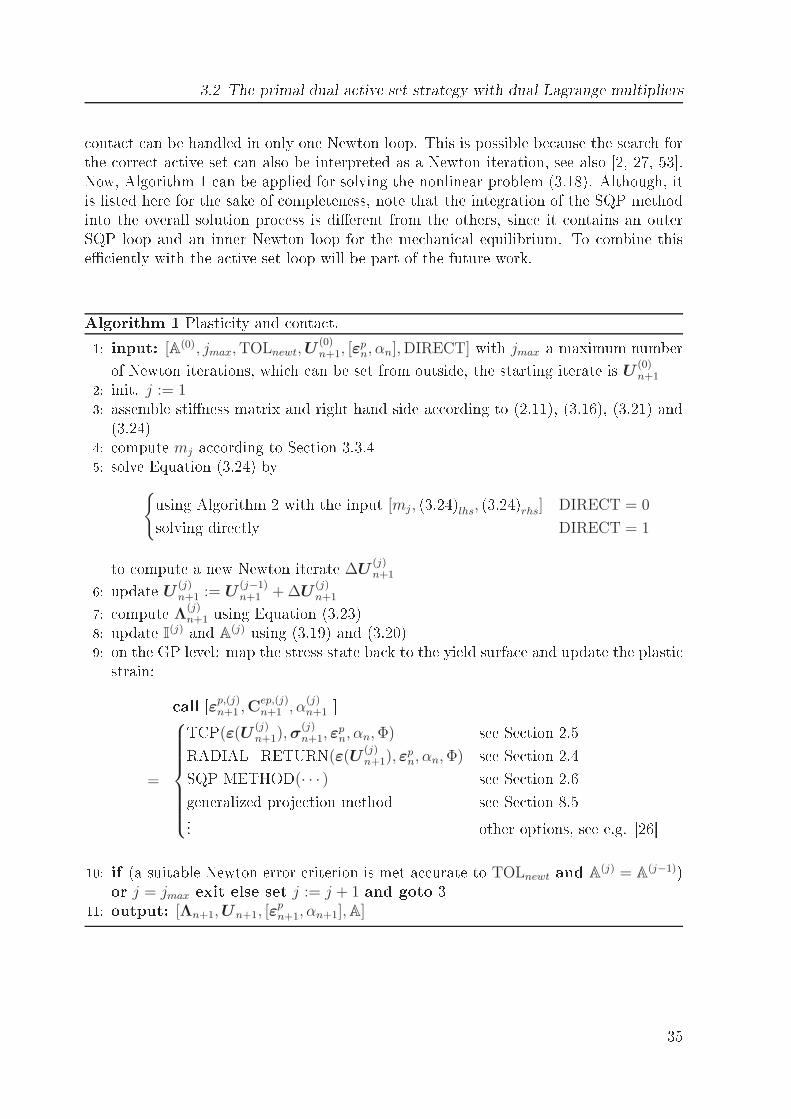
3.2 The primal dual a tive set strategy with dual Lagrange multipliers onta t an be handled in only one Newton loop. This is possible be ause the sear h forthe orre t a tive set an also be interpreted as a Newton iteration, see also [2, 27, 53.Now, Algorithm 1 an be applied for solving the nonlinear problem (3.18). Although, itis listed here for the sake of ompleteness, note that the integration of the SQP methodinto the overall solution pro ess is dierent from the others, sin e it ontains an outerSQP loop and an inner Newton loop for the me hani al equilibrium. To ombine thise iently with the a tive set loop will be part of the future work.Algorithm 1 Plasti ity and onta t.1: input: [A(0), jmax,TOLnewt,U(0)n+1, [ε

pn, αn],DIRECT] with jmax a maximum numberof Newton iterations, whi h an be set from outside, the starting iterate is U (0)

n+12: init. j := 13: assemble stiness matrix and right hand side a ording to (2.11), (3.16), (3.21) and(3.24)4: ompute mj a ording to Se tion 3.3.45: solve Equation (3.24) byusing Algorithm 2 with the input [mj , (3.24)lhs, (3.24)rhs] DIRECT = 0solving dire tly DIRECT = 1to ompute a new Newton iterate ∆U

(j)n+16: update U (j)

n+1 := U(j−1)n+1 + ∆U

(j)n+17: ompute Λ

(j)n+1 using Equation (3.23)8: update I(j) and A(j) using (3.19) and (3.20)9: on the GP level: map the stress state ba k to the yield surfa e and update the plasti strain: all [εp,(j)

n+1 ,Cep,(j)n+1 , α

(j)n+1

=

TCP(ε(U(j)n+1),σ

(j)n+1, ε

pn, αn,Φ) see Se tion 2.5RADIAL_RETURN(ε(U

(j)n+1), ε

pn, αn,Φ) see Se tion 2.4SQP METHOD(· · · ) see Se tion 2.6generalized proje tion method see Se tion 8.5... other options, see e.g. [2610: if (a suitable Newton error riterion is met a urate to TOLnewt and A

(j) = A(j−1))or j = jmax exit else set j := j + 1 and goto 311: output: [Λn+1,Un+1, [ε

pn+1, αn+1],A]

35

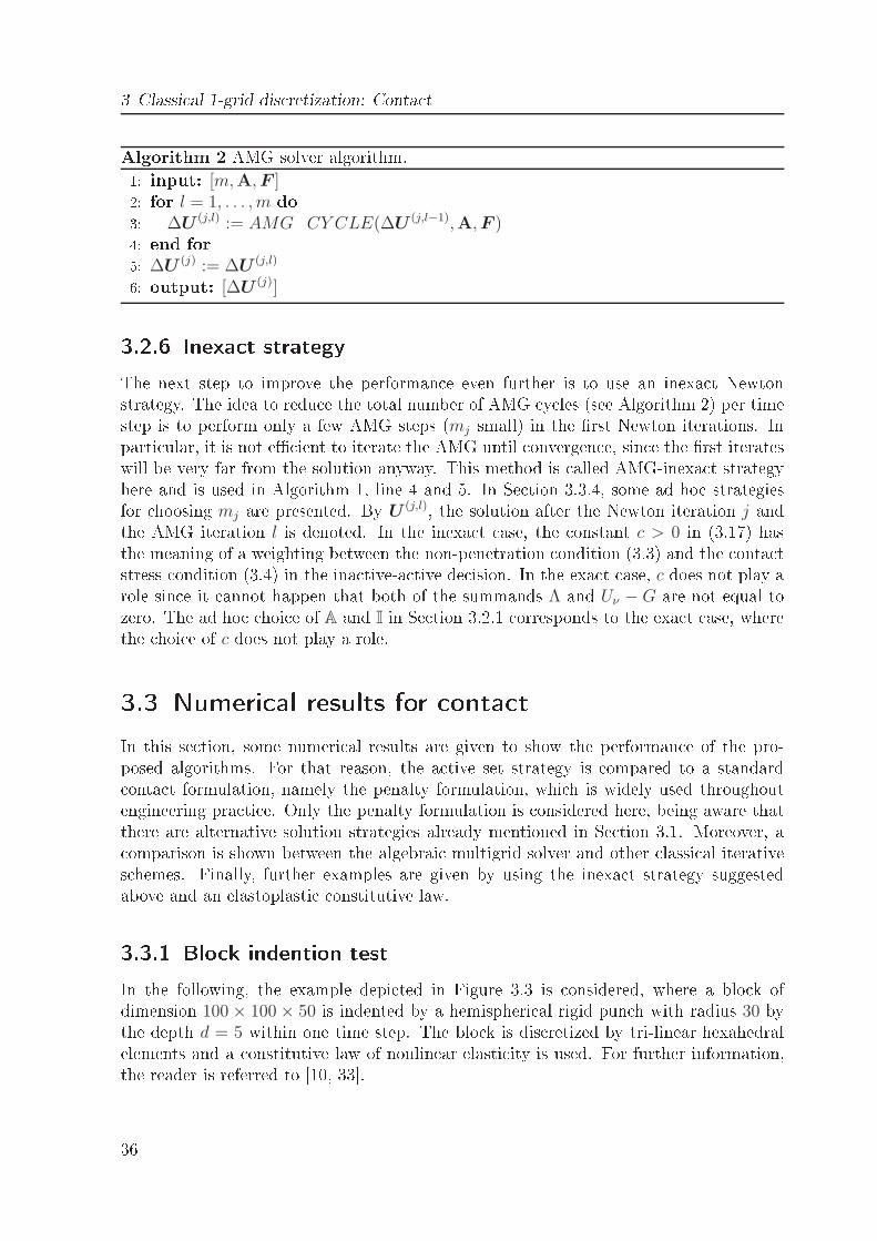
3 Classi al 1-grid dis retization: Conta tAlgorithm 2 AMG solver algorithm.1: input: [m,A,F ]2: for l = 1, . . . , m do3: ∆U (j,l) := AMG_CY CLE(∆U (j,l−1),A,F )4: end for5: ∆U (j) := ∆U (j,l)6: output: [∆U (j)]3.2.6 Inexa t strategyThe next step to improve the performan e even further is to use an inexa t Newtonstrategy. The idea to redu e the total number of AMG y les (see Algorithm 2) per timestep is to perform only a few AMG steps (mj small) in the rst Newton iterations. Inparti ular, it is not e ient to iterate the AMG until onvergen e, sin e the rst iterateswill be very far from the solution anyway. This method is alled AMG-inexa t strategyhere and is used in Algorithm 1, line 4 and 5. In Se tion 3.3.4, some ad ho strategiesfor hoosing mj are presented. By U (j,l), the solution after the Newton iteration j andthe AMG iteration l is denoted. In the inexa t ase, the onstant c > 0 in (3.17) hasthe meaning of a weighting between the non-penetration ondition (3.3) and the onta tstress ondition (3.4) in the ina tive-a tive de ision. In the exa t ase, c does not play arole sin e it annot happen that both of the summands Λ and Uν − G are not equal tozero. The ad ho hoi e of A and I in Se tion 3.2.1 orresponds to the exa t ase, wherethe hoi e of c does not play a role.3.3 Numeri al results for onta tIn this se tion, some numeri al results are given to show the performan e of the pro-posed algorithms. For that reason, the a tive set strategy is ompared to a standard onta t formulation, namely the penalty formulation, whi h is widely used throughoutengineering pra ti e. Only the penalty formulation is onsidered here, being aware thatthere are alternative solution strategies already mentioned in Se tion 3.1. Moreover, a omparison is shown between the algebrai multigrid solver and other lassi al iteratives hemes. Finally, further examples are given by using the inexa t strategy suggestedabove and an elastoplasti onstitutive law.3.3.1 Blo k indention testIn the following, the example depi ted in Figure 3.3 is onsidered, where a blo k ofdimension 100× 100× 50 is indented by a hemispheri al rigid pun h with radius 30 bythe depth d = 5 within one time step. The blo k is dis retized by tri-linear hexahedralelements and a onstitutive law of nonlinear elasti ity is used. For further information,the reader is referred to [10, 33.36

3.3 Numeri al results for onta t

X

Y

ZFigure 3.3: Setting of the onta t problem with rigid tool.Table 3.1: Comparison of results with de reasing penalty fa tor and a tive set strategy(ASeS).method displa ement dy,min Mises equiv. stress σmax

ρ = 105 -2.79 5665ρ = 107 -4.86 8370ρ = 109 -4.89 8399ASeS -4.99 83983.3.2 Comparison of both onta t approa hes in onne tion withAMGIn this se tion, the a tive set strategy is ompared with a standard penalty approa h.The penalty method an be formulated for the potential onta t nodes p ∈ S:

[F int(U)]⊤p ·N p + ρ(U p ·N p −Gp)+ = 0, p ∈ SThus, the penetration in the normal dire tion is penalized by the arti ial spring for ewith the spring rate ρ. This onstant must be of signi ant size (108− 1010 are ommonvalues in metal forming simulation) to avoid too large penetration of the bodies andensure high a ura y. Figure 3.4 and Table 3.1 illustrate the mentioned behavior.Unfortunately, the need for a large penalty value ρ is ontradi tory to the requirementsof iterative solvers. The penalty fa tor deteriorates the ondition numbers of the emergingequation systems, and thus leads to bad onvergen e rates of the iterative solvers. Thisproblem an be signi antly improved by using the primal-dual a tive set strategy asillustrated below. Figure 3.5 shows the onvergen e histories for the solution of the37

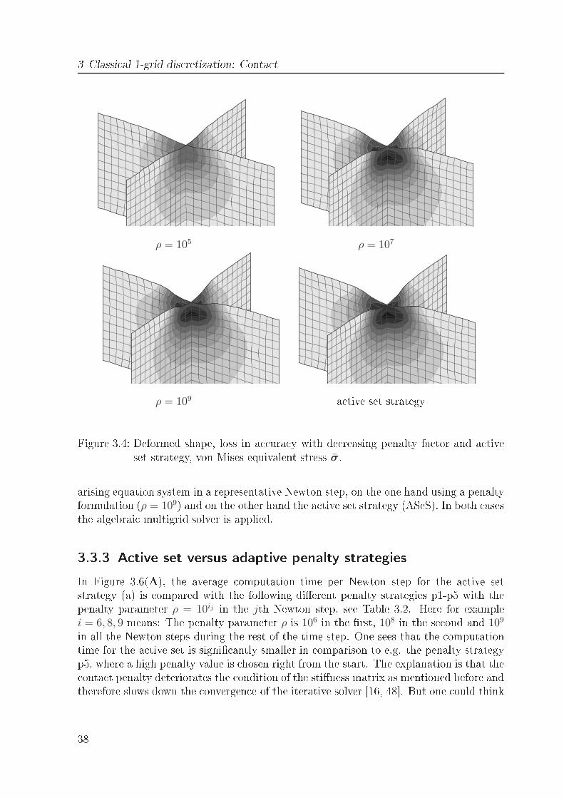
3 Classi al 1-grid dis retization: Conta t

ρ = 105 ρ = 107

ρ = 109 a tive set strategyFigure 3.4: Deformed shape, loss in a ura y with de reasing penalty fa tor and a tiveset strategy, von Mises equivalent stress σ.arising equation system in a representative Newton step, on the one hand using a penaltyformulation (ρ = 109) and on the other hand the a tive set strategy (ASeS). In both asesthe algebrai multigrid solver is applied.3.3.3 A tive set versus adaptive penalty strategiesIn Figure 3.6(A), the average omputation time per Newton step for the a tive setstrategy (a) is ompared with the following dierent penalty strategies p1-p5 with thepenalty parameter ρ = 10ij in the jth Newton step, see Table 3.2. Here for examplei = 6, 8, 9 means: The penalty parameter ρ is 106 in the rst, 108 in the se ond and 109in all the Newton steps during the rest of the time step. One sees that the omputationtime for the a tive set is signi antly smaller in omparison to e.g. the penalty strategyp5, where a high penalty value is hosen right from the start. The explanation is that the onta t penalty deteriorates the ondition of the stiness matrix as mentioned before andtherefore slows down the onvergen e of the iterative solver [16, 48. But one ould think38

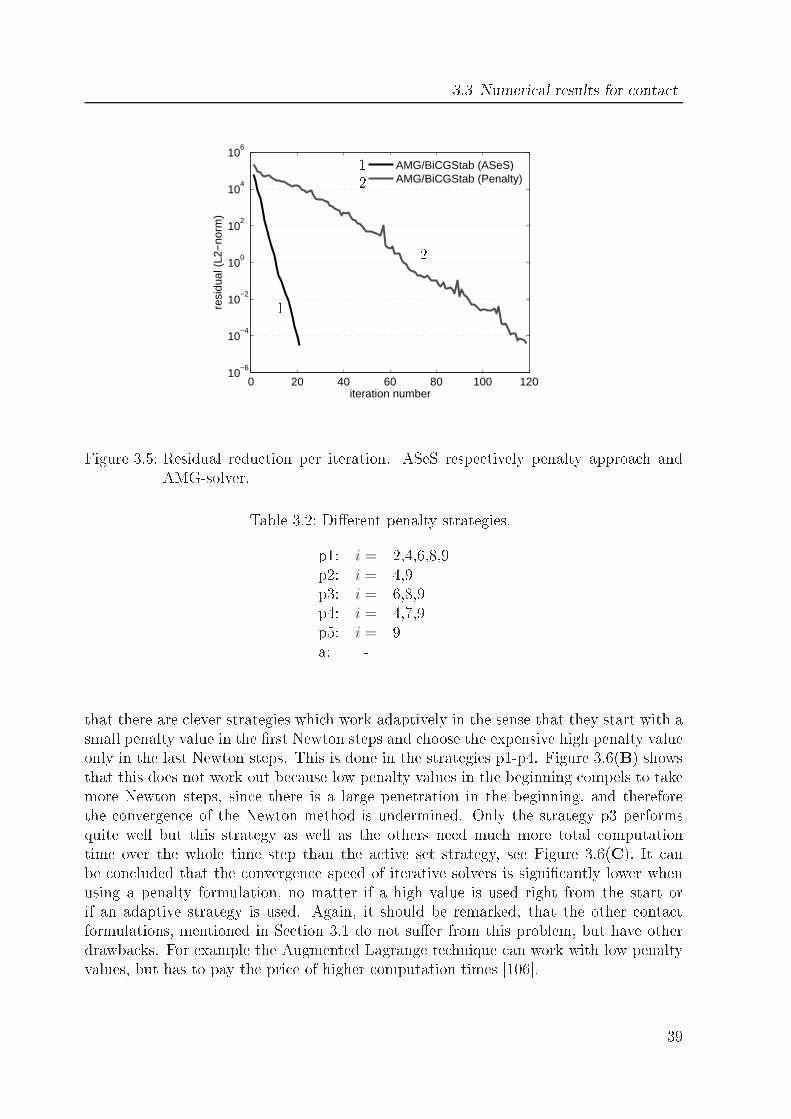
3.3 Numeri al results for onta t

0 20 40 60 80 100 12010

−6

10−4

10−2

100

102

104

106

iteration number

resi

dual

(L2

−no

rm)

AMG/BiCGStab (ASeS)AMG/BiCGStab (Penalty)

12 21Figure 3.5: Residual redu tion per iteration. ASeS respe tively penalty approa h andAMG-solver.Table 3.2: Dierent penalty strategies.p1: i = 2,4,6,8,9p2: i = 4,9p3: i = 6,8,9p4: i = 4,7,9p5: i = 9a: -that there are lever strategies whi h work adaptively in the sense that they start with asmall penalty value in the rst Newton steps and hoose the expensive high penalty valueonly in the last Newton steps. This is done in the strategies p1-p4. Figure 3.6(B) showsthat this does not work out be ause low penalty values in the beginning ompels to takemore Newton steps, sin e there is a large penetration in the beginning, and thereforethe onvergen e of the Newton method is undermined. Only the strategy p3 performsquite well but this strategy as well as the others need mu h more total omputationtime over the whole time step than the a tive set strategy, see Figure 3.6(C). It anbe on luded that the onvergen e speed of iterative solvers is signi antly lower whenusing a penalty formulation, no matter if a high value is used right from the start orif an adaptive strategy is used. Again, it should be remarked, that the other onta tformulations, mentioned in Se tion 3.1 do not suer from this problem, but have otherdrawba ks. For example the Augmented Lagrange te hnique an work with low penaltyvalues, but has to pay the pri e of higher omputation times [106. 39

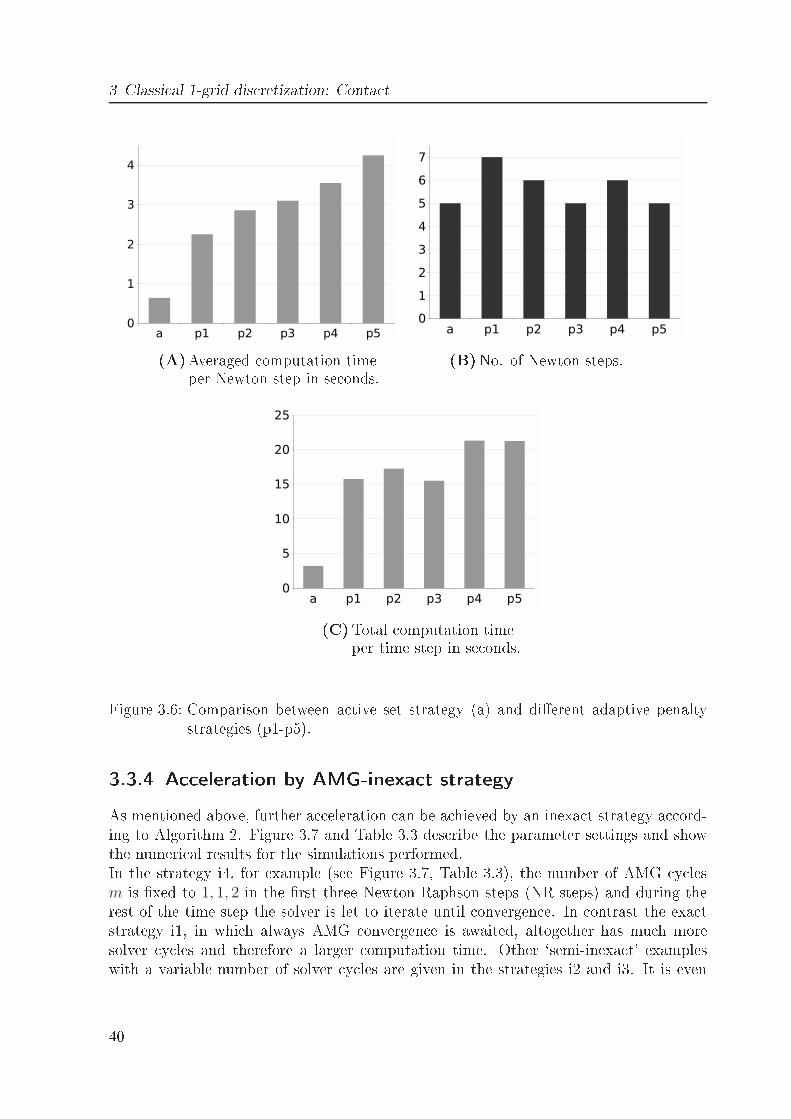
3 Classi al 1-grid dis retization: Conta t

(A)Averaged omputation timeper Newton step in se onds. (B)No. of Newton steps.

(C)Total omputation timeper time step in se onds.Figure 3.6: Comparison between a tive set strategy (a) and dierent adaptive penaltystrategies (p1-p5).3.3.4 A eleration by AMG-inexa t strategyAs mentioned above, further a eleration an be a hieved by an inexa t strategy a ord-ing to Algorithm 2. Figure 3.7 and Table 3.3 des ribe the parameter settings and showthe numeri al results for the simulations performed.In the strategy i4, for example (see Figure 3.7, Table 3.3), the number of AMG y lesm is xed to 1, 1, 2 in the rst three Newton-Raphson steps (NR steps) and during therest of the time step the solver is let to iterate until onvergen e. In ontrast the exa tstrategy i1, in whi h always AMG onvergen e is awaited, altogether has mu h moresolver y les and therefore a larger omputation time. Other `semi-inexa t' exampleswith a variable number of solver y les are given in the strategies i2 and i3. It is even40

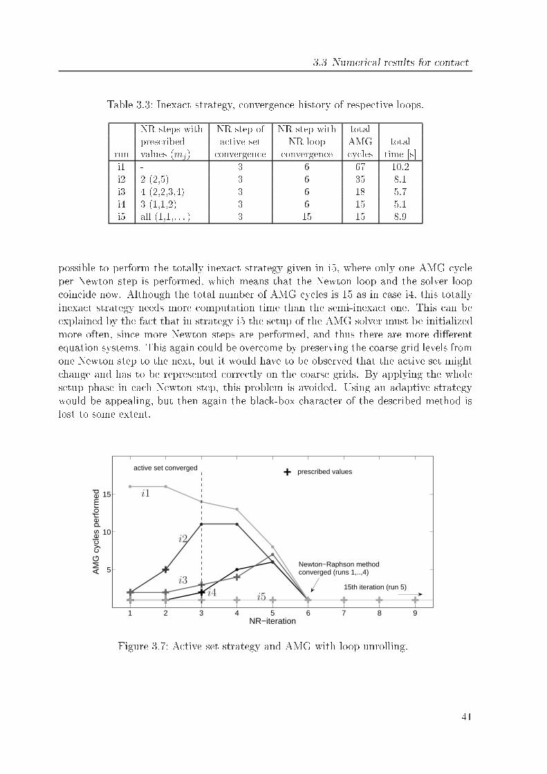
3.3 Numeri al results for onta tTable 3.3: Inexa t strategy, onvergen e history of respe tive loops.NR steps with NR step of NR step with totalpres ribed a tive set NR loop AMG totalrun values (mj) onvergen e onvergen e y les time [si1 - 3 6 67 10.2i2 2 (2,5) 3 6 35 8.1i3 4 (2,2,3,4) 3 6 18 5.7i4 3 (1,1,2) 3 6 15 5.1i5 all (1,1,. . . ) 3 15 15 8.9possible to perform the totally inexa t strategy given in i5, where only one AMG y leper Newton step is performed, whi h means that the Newton loop and the solver loop oin ide now. Although the total number of AMG y les is 15 as in ase i4, this totallyinexa t strategy needs more omputation time than the semi-inexa t one. This an beexplained by the fa t that in strategy i5 the setup of the AMG solver must be initializedmore often, sin e more Newton steps are performed, and thus there are more dierentequation systems. This again ould be over ome by preserving the oarse grid levels fromone Newton step to the next, but it would have to be observed that the a tive set might hange and has to be represented orre tly on the oarse grids. By applying the wholesetup phase in ea h Newton step, this problem is avoided. Using an adaptive strategywould be appealing, but then again the bla k-box hara ter of the des ribed method islost to some extent.

1 2 3 4 5 6 7 8 9

5

10

15

NR−iteration

AM

G c

ycle

s pe

rfor

med

Newton−Raphson methodconverged (runs 1,..,4)

15th iteration (run 5)

active set converged + prescribed values

i1

i2

i3i4 i5Figure 3.7: A tive set strategy and AMG with loop unrolling.

41

3 Classi al 1-grid dis retization: Conta t3.4 SummaryIt an be on luded that the proposed onta t algorithm allows to apply fast iterativesolvers on nonlinear problems in a very e ient way. It was shown, that the dis ussedalgebrai multigrid methods signi antly gain in e ien y in omparison to standardpenalty approa hes when used in ombination with a primal-dual a tive set strategy. Itwill be part of the future work to ompare this method with the other onta t formulationsmentioned in Se tion 3.1. Furthermore it was shown that omputation time an be furtherde reased by merging the otherwise nested loops of ea h method into a single solver loopby the des ribed inexa t strategies. The theory explained exhibits the hara ter of themethod and a way to implement the method in a pra ti al manner into a FE pa kage.The study is based on a very simple approa h for the algebrai multigrid in order topreserve the bla k-box appli ability of the method to a maximum extent.The remark has to be made, that there are many reasons for a bad ondition numberof the system matrix, not only the onta t penalty. For example, also bu kling tends todeteriorate the ondition number but it is not addressed in this work. The reason is thathere, it is assumed, that a metal forming pro ess whi h is near to bu kling or any kindof bifur ation behavior 1 belongs already to the ill- ontrolled pro esses whi h are not tobe simulated here. Nevertheless, it stays part of the future work to1. validate this assumption arefully and, if it proves to be true,2. to in orporate the dete tion of undesired bifur ation behavior into the algorithmsof this work.

1to su h an extent that the ondition number gets signi antly deteriorated (at the bifur ation point,the Ja obian is singular)42

4 Dynami onta tThe e ient modeling of dynami , thin-walled, large deformation 3D onta t problemsis still a hallenge in nonlinear impli it stru tural analysis.4.1 Introdu tionA great number of onta t algorithms developed in the past enfor e the onta t on-straints at spe i ollo ation points. Using a node-to-segment approa h, the main ideais that a spe i node on the slave side must not penetrate the opposing master sidesegment. Although this approa h is quite popular and available in numerous ommer ialnite element odes, the robustness of these methods is still a limitation in ertain appli- ations. So- alled single pass algorithms do not satisfy the onta t pat h test [89, wherea at onta t surfa e should be able to transmit a spatially onstant onta t pressure fromone body to the other. Using low order nite elements, the nonsmooth representationof the real geometry will have a signi ant inuen e on the performan e of a node-to-segment approa h. It will ause jumps in the onta t for es on e a slave node slides othe onta ting master segment. Various smoothing algorithms have been proposed toover ome these de ien ies, e.g. [88, 91, 100. Proposed two-pass algorithms indeed passthe onta t pat h test for 2D and some 3D mesh ongurations, but they suer in turnfrom lo king.Due to these drawba ks of the lassi al onta t algorithms, the resear h on segment-to-segment onta t strategies be ame quite a tive in re ent years. Most of these newapproa hes use the so- alled mortar method, initially introdu ed as a domain de ompo-sition method by Bernardi and o-workers [14. The reader is referred to [9, 11, 12 andthe referen es therein for an overview of the mortar method in the ontext of onta tproblems. Yang et al. [115 des ribe a onta t method for two dimensional large deforma-tion fri tional sliding. Puso and Laursen [92, 93 develop a mortar segment-to-segment onta t method for large deformation solid me hani s for three dimensional appli ations.M Devitt and Laursen [82 introdu e an intermediate mortar surfa e to proje t the on-ta t onditions between two onta ting surfa es. A 2D mortar formulation was also usedby Fis her and Wriggers [38.In this formulation, a primal-dual a tive set strategy [2, 27, 53 is used whi h allows toenfor e the onta t onstraints without any additional parameter. The su ess of thisstrategy is based on the introdu tion of dual Lagrange multipliers [107 to dis retize the onta t pressure. Following the approa h des ribed in Hüeber and Wohlmuth [57, oneends up with an algebrai stru ture of the problem whi h allows to lo ally eliminate the43

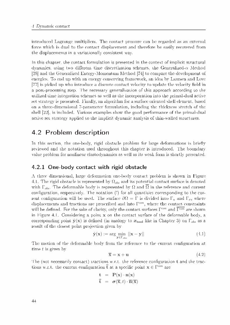
4 Dynami onta tintrodu ed Lagrange multipliers. The onta t pressure an be regarded as an externalfor e whi h is dual to the onta t displa ement and therefore be easily re overed fromthe displa ements in a variationally onsistent way.In this hapter, the onta t formulation is presented in the ontext of impli it stru turaldynami s, using two dierent time dis retization s hemes, the Generalized-α Method[28 and the Generalized Energy-Momentum Method [74 to ompare the development ofenergies. To end up with an energy onserving framework, an idea by Laursen and Love[77 is pi ked up who introdu e a dis rete onta t velo ity to update the velo ity eld ina post-pro essing step. The ne essary generalization of this approa h a ording to theutilized time integration s hemes as well as the in orporation into the primal-dual a tiveset strategy is presented. Finally, an algorithm for a surfa e oriented shell element, basedon a three-dimensional 7-parameter formulation, in luding the thi kness stret h of theshell [22, is in luded. Various examples show the good performan e of the primal-duala tive set strategy applied to the impli it dynami analysis of thin-walled stru tures.4.2 Problem des riptionIn this se tion, the one-body, rigid obsta le problem for large deformations is brieyreviewed and the notation used throughout this hapter is introdu ed. The boundaryvalue problem for nonlinear elastodynami s as well as its weak form is shortly presented.4.2.1 One-body onta t with rigid obsta leA three dimensional, large deformation one-body onta t problem is shown in Figure4.1. The rigid obsta le is represented by Ωobs and its potential onta t surfa e is denotedwith Γobs. The deformable body is represented by Ω and Ω in the referen e and urrent onguration, respe tively. The notation (·) for all quantities orresponding to the ur-rent onguration will be used. The surfa e ∂Ω = Γ is divided into Γu and Γσ, wheredispla ements and tra tions are pres ribed and into Γcon, where the onta t onstraintswill be dened. For the sake of larity, only the onta t surfa es Γcon and Γcon are shownin Figure 4.1. Considering a point x on the onta t surfa e of the deformable body, a orresponding point y(x) is dened (in analogy to xtool like in Chapter 3) on Γobs as aresult of the losest point proje tion given byy(x) := arg min

y∈Γobs

||x− y|| (4.1)The motion of the deformable body from the referen e to the urrent onguration attime t is given byx = x + u (4.2)The (not ne essarily onta t) tra tions w.r.t. the referen e onguration t and the tra -tions w.r.t. the urrent onguration t at a spe i point x ∈ Γcon are

t = P(x) · n(x)

t = σ(x, t) · n(x)44

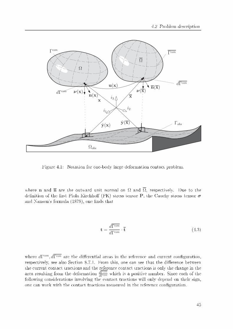
4.2 Problem des riptionPSfrag repla ementsΓcon

Γcon

Γobs

Ω

Ω

Ωobs

u(x)

xx

y(x)y(x)

ν(x) ν(x)n(x)

n(x)dΓcon

dΓcon

i1i2

i3

Figure 4.1: Notation for one-body large deformation onta t problem.where n and n are the outward unit normal on Ω and Ω, respe tively. Due to thedenition of the rst Piola Kir hho (PK) stress tensor P, the Cau hy stress tensor σand Nanson's formula (1878), one nds thatt =

dΓcon

dΓcon· t (4.3)

where dΓcon, dΓcon are the dierential areas in the referen e and urrent onguration,respe tively, see also Se tion 8.7.1. From this, one an see that the dieren e betweenthe urrent onta t tra tions and the referen e onta t tra tions is only the hange in thearea resulting from the deformation dΓcon

dΓcon whi h is a positive number. Sin e ea h of thefollowing onsiderations involving the onta t tra tions will only depend on their sign,one an work with the onta t tra tions measured in the referen e onguration. 45

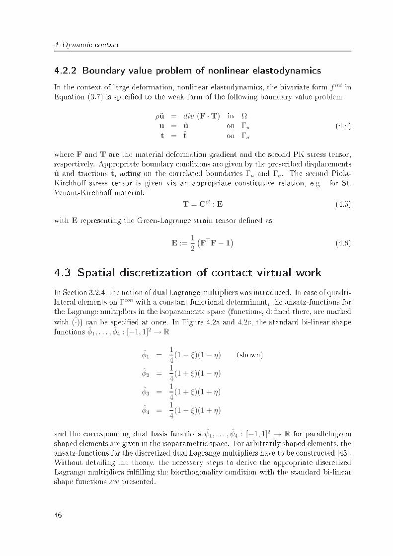
4 Dynami onta t4.2.2 Boundary value problem of nonlinear elastodynami sIn the ontext of large deformation, nonlinear elastodynami s, the bivariate form f int inEquation (3.7) is spe ied to the weak form of the following boundary value problemρu = div (F ·T) in Ωu = u on Γu

t = t on Γσ

(4.4)where F and T are the material deformation gradient and the se ond PK stress tensor,respe tively. Appropriate boundary onditions are given by the pres ribed displa ementsu and tra tions t, a ting on the orrelated boundaries Γu and Γσ. The se ond Piola-Kir hho stress tensor is given via an appropriate onstitutive relation, e.g. for St.Venant-Kir hho material:

T = Cel : E (4.5)with E representing the Green-Lagrange strain tensor dened asE :=

1

2

(

F⊤F− 1) (4.6)4.3 Spatial dis retization of onta t virtual workIn Se tion 3.2.4, the notion of dual Lagrange multipliers was introdu ed. In ase of quadri-lateral elements on Γcon with a onstant fun tional determinant, the ansatz-fun tions forthe Lagrange multipliers in the isoparametri spa e (fun tions, dened there, are markedwith (·)) an be spe ied at on e. In Figure 4.2a and 4.2 , the standard bi-linear shapefun tions φ1, . . . , φ4 : [−1, 1]2 → R

φ1 =1

4(1− ξ)(1− η) (shown)

φ2 =1

4(1 + ξ)(1− η)

φ3 =1

4(1 + ξ)(1 + η)

φ4 =1

4(1− ξ)(1 + η)and the orresponding dual basis fun tions ψ1, . . . , ψ4 : [−1, 1]2 → R for parallelogramshaped elements are given in the isoparametri spa e. For arbitrarily shaped elements, theansatz-fun tions for the dis retized dual Lagrange multipliers have to be onstru ted [43.Without detailing the theory, the ne essary steps to derive the appropriate dis retizedLagrange multipliers fullling the biorthogonality ondition with the standard bi-linearshape fun tions are presented.46

4.3 Spatial dis retization of onta t virtual work4.3.1 Dis rete dual Lagrange multipliers for arbitrary shapedelementsDene with T and T = [−1, 1]2 a 4-noded element on the onta t boundary Γcon, givenin the physi al and the isoparametri spa e, respe tively. Furthermore byFT : T → T ⊂ R

3the element mapping su h that φi = φi FT is denoted. The aim is now to nd fun tionsψi su h that the biorthogonality ondition (3.10) holds element-wise on T ⊂ Γcon:

∫

T

ψiφj dT = δij

∫

T

φj dT (4.7)Therefore, one onstru ts the ansatz-fun tions for the Lagrange multipliers in the follow-ing way:ψi :=

∑

k

aikφk, with AT := aij := DT M−1T ∈ R

4×4 (4.8)and thereinDT := δij

∫

T

φjdT, MT :=

∫

T

φiφjdTthe desired diagonal matrix and the element mass matrix without density and sets ψi :=ψi F−1

T . Then one veries:∫

T

ψiφjdT =

∫

T

JψiφjdT

=

∫

T

J∑

k

aikφkφjdT

=∑

k

aik

∫

T

JφkφjdT

=∑

k

aik[MT ]kj

= [ATMT ]ij = [DT ]ijHerein J := JT := det(FT ) is the Ja obian of an element T . To further illustrate thispro edure, one dis rete ansatz-fun tion for the dual Lagrange multipliers for two dierentelement shapes is exemplarily al ulated. The rst one has a regular shape, resulting ina onstant Ja obian determinant J = const whereas the se ond one is of arbitrary shapewith J 6= const.PSfrag repla ementsUndistorted Element:

0 2 2 00 0 2 20 0 0 0

x1

x2

00

1

1

2

2 47

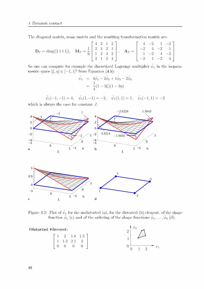
4 Dynami onta tThe diagonal matrix, mass matrix and the resulting transformation matrix are:DT = diag([1 1 1 1]), MT =

1

9

4 2 1 22 4 2 11 2 4 22 1 2 4

, AT =

4 −2 1 −2−2 4 −2 1

1 −2 4 −2−2 1 −2 4

So one an ompute for example the dis retized Lagrange multiplier ψ1 in the isopara-metri spa e [ξ, η] ∈ [−1, 1]2 from Equation (4.8):ψ1 = 4φ1 − 2φ2 + 1φ3 − 2φ4

=1

4(1− 3ξ)(1− 3η)

ψ1(−1,−1) = 4, ψ1(1,−1) = −2, ψ1(1, 1) = 1, ψ1(−1, 1) = −2whi h is always the ase for onstant J .which is always the case for constant J .

−10

1 −1

0

1

−4

−2

0

2

4

ηξ

−10

1 −1

0

1

−4

−2

0

2

4

ηξ

−10

1 −1

0

10

0.5

1

ηξ

4

−2

−2

1

@@

3.8214@

@@

−1.9035

1.3043

@@@

−2.6228

1

2

3

4

a b

c dFigure 4.2: Plot of ψ1 for the undistorted (a), for the distorted (b) element, of the shapefun tion φ1 ( ) and of the ordering of the shape fun tions φ1, . . . , φ4 (d).PSfrag repla ementsDistorted Element:

1 2 1.8 1.51 1.3 2.1 20 0 0 0

x1

x2

00

1

1

2

248

4.3 Spatial dis retization of onta t virtual workThe diagonal matrix and mass matrix are:DT = diag

0.16330.16420.11420.1133

, MT =

0.0781 0.0392 0.0154 0.03070.0392 0.0786 0.0310 0.01540.0154 0.0310 0.0453 0.02250.0307 0.0154 0.0225 0.0447

The resulting transformation matrix is:AT =

3.8214 −1.9035 1.3043 −2.6228−1.9132 3.8118 −2.6075 1.3109

0.9116 −1.8133 4.6024 −2.3161−1.8199 0.9050 −2.2992 4.6280

Again, one an ompute the dis retized Lagrange multiplier ψ1:ψ1 = 3.8214φ1 − 1.9035φ2 + 1.3043φ3 − 2.6228φ4

ψ1(−1,−1) = 3.8214 ψ1(1,−1) = −1.9035 ψ1(1, 1) = 1.3043 ψ1(−1, 1) = −2.6228In Figure 4.2a and 4.2b the ansatz-fun tions ψ1 is shown for the undistorted and the dis-torted element, respe tively. The general stru ture of the interpolation fun tions remainsthe same, but the basis values at the nodes of the elements vary.4.3.2 Semidis rete initial value problemStarting from the weak form of the nonlinear dynami onta t problem (4.4), the semidis- rete equation of motion is derived introdu ing the spatial dis retization via nite ele-ments.MρU + CU + F int(U) + F c = F ext (4.9)Herein, Mρ represents the mass matrix, C the vis ous damping matrix, F int(U) thedeformation dependent internal for es, F c the onta t for es and F ext the external for es.

U are the nodal velo ities and U the nodal a elerations. Consequently, the inertia for esand damping for es are given by MρU and CU , respe tively. The damping matrix isassumed to be a linear ombination of the mass matrix and the elasti stiness matrixA whi h orresponds to the so- alled proportional or Rayleigh damping.After appropriate ordering of the variables, the onta t for es an be expressed in exa tlythe same manner as in Equation (3.9)

F c = B Λ (4.10)It is worth noting that the determination of the entries of B an be performed in thereferen e onguration. This will have the advantage that the weighting fa tors have tobe al ulated only on e, thus no linearization is ne essary for the al ulation of B. 49

4 Dynami onta t4.4 Time dis retizationTo integrate the semidis rete problem (4.9), the time interval of interest [0, T ] is subdi-vided into typi al time intervals [tn, tn+1] with the orresponding time step ∆t = tn+1−tn.Given the state variables Un, Un and Un at time tn, Equation (4.9) is solved in an im-pli it way to obtain the solution of the state variables Un+1, Un+1 and Un+1 at the endof ea h time step. To redu e the set of unknown variables to the displa ements Un+1,the lassi al Newmark approximations are used.Un+1(Un+1) = Un + ∆t Un + 1−2β

2∆t2 Un + β∆t2 Un+1

Un+1(Un+1) = Un + (1− γ)∆t Un + γ∆t Un+1

(4.11)Equivalently the velo ities and a elerations are rewritten in terms of the displa ementat time tn+1.Un+1(Un+1) = γ

β∆t(Un+1 −Un)−

(

γβ− 1)

Un −(

γ2β− 1)

∆t Un

Un+1(Un+1) = 1β∆t2

(Un+1 −Un)− 1β∆tUn −

(

12β− 1)

Un

(4.12)In the following, two slightly dierent time integration s hemes are des ribed, both basedon the given Newmark s heme. The Generalized-α Method (Gen-α), originally proposedfor linear dynami al systems by Chung and Hulbert [28 and the Generalized Energy-Momentum Method (GEMM) developed by Kuhl and Criseld [73 for trusses and lateradapted for nonlinear shell dynami s by Kuhl and Ramm [74. Both methods apply thesemidis rete equation of motion (4.9) at a generalized mid-point ongurationMρ Un+1−αm

+ C Un+1−αf+ F int

n+1−αf+ F c

n+1−αf= F ext

n+1−αf(4.13)des ribed via two shift parameters αm and αf . Herein, the subs ripts denote the timedis rete ombinations of the a elerations, velo ities, displa ements, internal, onta t andexternal for es.

Un+1−αm= (1− αm)Un+1 + αmUn

Un+1−αf= (1− αf)Un+1 + αf Un

Un+1−αf= (1− αf)Un+1 + αfUn

F intn+1−αf

=

(1− αf)Fintn+1 + αfF

intn for Gen-α

F int ((1− αf)Un+1 + αfUn) for GEMMF ext

n+1−αf= (1− αf)F

extn+1 + αfF

extn

(4.14)The ru ial dieren e between the Generalized-α Method and the Generalized Energy-Momentum Method is the al ulation of the internal for es at the generalized mid-point onguration. In the Generalized-α Method, the internal for es are approximated usingthe general trapezoidal rule, whereas in the General Energy-Momentum Method, theinternal for es are al ulated at the mid-point onguration. This is essential for this50

4.4 Time dis retizationmethod and will have signi ant inuen e on the derivation of the deformation dependentalgorithmi tangential stiness matrix, whi h will be dis ussed separately when des ribingthe surfa e oriented shell element in Se tion 4.5. A ording to Equation (4.10), the ontribution of the onta t for es in Equation (4.13) an be expressed asF c

n+1−αf= B Λn+1−αf

(4.15)Combining the approximations of the velo ities and a elerations (4.12) and (4.14) withthe equation of motion (4.13) together with (4.15) yields the ee tive stru tural equationwhi h is nonlinear in the unknown displa ements Un+1

Z(Un+1) := F intn+1−αf

(Un+1) +1− αm

β∆t2Mρ Un+1 +

(1− αf)γ

β∆tC Un+1 −

H(Un, Un, Un) + B Λn+1−αf− F ext

n+1−αf= 0 (4.16)where H(Un, Un, Un), the history term, is only dependent on the given state variablesat time tn.

H(Un, Un, Un) := Mρ

[

1− αm

β∆t2Un +

1− αm

β∆tUn +

1− αm − 2β

2βUn

]

+ (4.17)C

[

(1− αf)γ

β∆tUn +

(1− αf)γ − ββ

Un +(γ − 2β)(1− αf )

2β∆tUn

]4.4.1 Linearization and iterative solution strategyThe nonlinearity of the ee tive stru tural equation needs an iterative solution pro edure.Therefore Equation (4.16) is linearized in dire tion of∆U (j+1) = U

(j+1)n+1 −U (j)

n+1 (4.18)and the Newton-Raphson iteration te hnique is applied. This leads to the ee tive iter-ative stru tural equationJ(j)∆U (j+1) = −Z(U

(j)n+1) (4.19)where J(j) is the ee tive algorithmi tangential stiness matrix

J(j) :=∂F int(Un+1−αf

(Un+1))

∂Un+1

+1− αm

β∆t2Mρ +

(1− αf )γ

β∆tC (4.20)and Z(U

(j)n+1) are the out-of-balan e for es at iteration step j. Now, all these matri esare sorted a ording to the denition of the subsets N and S, and the onta t term

B Λn+1−αfis put onto the left hand side. With the ordering (3.11), one arrives at thefollowing in remental representation of the ee tive stru tural Equation (4.16)

[

JNN JNS 0

JSN JSS D

](j)

∆UN

∆U S

∆Λn+1−αf

(j+1)

= −[

ZN

ZS + DΛn+1−αf

](j) (4.21)51

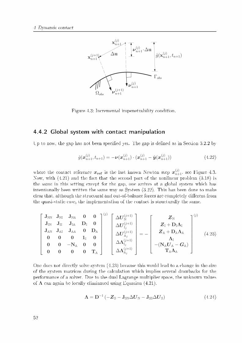
4 Dynami onta tPSfrag repla ementsν

(j+1)n+1

ν(j)n+1

ν(j)n+1 ·∆u

Ωobs

∆u g(x(j)n+1, tn+1)

x(j)n+1

x(j+1)n+1

Γobs

Figure 4.3: In remental impenetrability ondition.4.4.2 Global system with onta t manipulationUp to now, the gap has not been spe ied yet. The gap is dened as in Se tion 3.2.2 byg(x

(j)n+1, tn+1) = −ν(x

(j)n+1) · (x(j)

n+1 − y(x(j)n+1)) (4.22)where the onta t referen e xref is the last known Newton step x(j)

n+1, see Figure 4.3.Now, with (4.21) and the fa t that the se ond part of the nonlinear problem (3.18) isthe same in this setting ex ept for the gap, one arrives at a global system whi h hasintentionally been written the same way as System (3.22). This has been done to make lear that, although the stru tural and out-of-balan e for es are ompletely dierent fromthe quasi-stati ase, the implementation of the onta t is stru turally the same.

JNN JNI JNA 0 0

JIN JII JIA DI 0

JAN JAI JAA 0 DA

0 0 0 1I 0

0 0 −NA 0 0

0 0 0 0 TA

(j)

∆U(j+1)N

∆U(j+1)Ij

∆U(j+1)Aj

∆Λ(j+1)Ij

∆Λ(j+1)Aj

= −

ZN

ZI + DIΛI

ZA + DAΛA

ΛI

−(NAUA −GA)TAΛA

(j) (4.23)One does not dire tly solve system (4.23) be ause this would lead to a hange in the sizeof the system matri es during the al ulation whi h implies several drawba ks for theperforman e of a solver. Due to the dual Lagrange multiplier spa e, the unknown valuesof Λ an again be lo ally eliminated using Equation (4.21).

Λ = D−1 (−ZS − JSN∆UN − JSS∆U S) (4.24)52

4.5 Spatial dis retization by a nite shell elementA stati ondensation yields the redu ed system

JNN JNI JNA

JIN JII JIA

0 0 −NA

TAJAN TAJAI TAJAA

(j)

∆U(j+1)N

∆U(j+1)Ij

∆U(j+1)Aj

= −

ZN

ZI

GA −NAUA

TAZA

(j) (4.25)to be solved in ea h Newton step j. As mentioned before, the size of this system remains onstant during the al ulation and is determined only by the nite element dis retiza-tion. In the present approa h, the onta t for es are al ulated from the displa ementsin a variationally onsistent way in a post pro essing step. The geometri onta t on-straint of an a tive node in Aj is dire tly introdu ed as a Diri hlet boundary onditionin a weak integral sense. Therefore no user dened parameter like a penalty parameteris needed in this approa h.4.5 Spatial dis retization by a nite shell elementThe spatial dis retization of the deformable body is realized by an eight noded, hexahe-dral surfa e oriented nite shell element of the Reissner/Mindlin type. Its formulation isbased on the shell element presented by Bü hter et al. ([22, [23). A detailed des riptionand several enhan ements to this shell formulation are presented by Bis ho [15.For the appli ation to onta t problems, the original des ription of the shell geometrywas modied. In the original formulation, the kinemati s of the nonlinear shell element isdes ribed via a displa ement eld of the shell mid-surfa e plus an extensible shell dire toreld. Having the nite element nodes situated in the shell mid-surfa e, the formulationof onta t problems be omes quite ompli ated as all the onta t integrals have to be al ulated with respe t to the real surfa e of the shell body. Thus, onta t for es a tingon the a tual shell surfa e have to be transmitted to the degrees of freedom living in themid-surfa e. Although this approa h has been su essfully applied for a lassi al node-to-segment onta t formulation by Gee [44, the geometry des ription is reformulated,leading to a surfa e-oriented shell element. With the nite element nodes now lying onthe shell surfa e, one an apply the onta t approa h without any further modi ationas for any standard hexahedral solid element.4.6 Energy onservation for fri tionless onta tIt is known [52, 59, 75 that the appli ation of the presented time integration algorithms,without any spe ial treatment of the onta t onstraints will not result in an energy onservative method. Dealing with fri tionless dynami onta t problems, it is wellknown that the fulllment of the so- alled persisten y ondition(λ(x, t) · ν(x, t))g(x, t) = 0 (4.26)53

4 Dynami onta twill lead to an energy onserving s heme. Here, the gap g is the urrent gapg(x, t) = −ν(x) · (x− y(x)), t ∈ [0, T ]instead of the gap in Equation (4.22). Considering the time ontinuous ase, the per-sisten y ondition is automati ally fullled if the Karush-Kuhn-Tu ker onditions aresatised. Various strategies to fulll this additional onstraint (e.g. [5 and [76) havethe drawba k of violating the geometri admissibility instead. This work follows the ideaof Laursen and Love [77 by introdu ing a dis rete onta t velo ity V c into the velo ityupdate:

Uupd

n+1 = Un+1 + V cThis additional term is motivated by the fa t that the analyti al solution of a simple one-dimensional onta t problem is hara terized by dis rete velo ity jumps o urring withinone dis rete time step. Without an expli it omplian e of an algorithmi persisten y ondition, this strategy allows the treatment of the geometri onta t onstraints inan unmodied manner. Thus the impenetrability ondition is still satised in a weakintegral sense. The framework des ribed in [77 onsiders the lassi al midpoint rule.This approa h is generalized a ording to the Generalized-α and the Generalized Energy-Momentum Method, leading to the following form of the velo ity update, see Equation(4.12)U

upd

n+1 =γ

β∆t(Un+1 −Un)−

(

γ

β− 1

)

Un −(

γ

2β− 1

)

∆t Un + V c (4.27)To derive the energy onservation onditions, a spe ial variation of the dis retized prob-lem (4.13) is performed, ex luding the damping term and the external for es sin e energy onservation only makes sense in this setting. Due to the orre tion term, the dynami equilibriumMρ

(

Un+1−αm− 1− αm

γ∆tV c

)

+ F intn+1−αf

+ F cn+1−αf

= 0 (4.28)is solved and this equation is multiplied with (see Equation (4.27))∆U = ∆U upd − β∆t

γV c (4.29)with

∆U upd :=β∆t

γ

[

Uupd

n+1 +

(

γ

β− 1

)

Un +

(

γ

2β− 1

)

∆t Un

] (4.30)In the absen e of onta t, the hange in total energy an be expressed asU

⊤

n+1−αmMρ∆U

upd + (F intn+1−αf

)⊤∆U = ∆Etot (4.31)In the following, only the terms arising from the onta t for es and the dis rete velo ityupdate are onsidered to arrive at a ondition whi h satises energy onservation for the onta t part. Therefore Equation (4.28) is multiplied with ∆U (Equation (4.29))0 = (4.28)lhs ·∆U = ∆Etot + ∆Enum54

4.6 Energy onservation for fri tionless onta twith the pure numeri al gain or loss of energy∆Enum := (4.32)(

−1− αm

γ∆t∆Uupd +

β(1− αm)

γ2V c − β∆t

γUn+1−αm

)⊤

MρVc + (F c

n+1−αf)⊤∆USo the ondition

∆Enum = 0 (4.33)guarantees energy onservation for the onta t part. Therefore, the total energy onser-vation depends on the used time integration s heme.After inserting all ne essary interpolation denitions into Equation (4.33) and after somealgebrai modi ations, one an express the onta t energy onservation ondition interms of known variables(

R1∆U +R2Un +R3Un +R4Vc)⊤

Mρ Vc + (F c

n+1−αf)⊤∆U = 0 (4.34)Herein the onstants Ri are dened as

R1 :=2(1− αm)

γ∆t, R2 := −(1− αm)

γ, R3 := −∆t

2γ(2β + αm − 1), R4 :=

β(1− αm)

γ2(4.35)Dene now the ve tor of nodal normal onta t for es Λν ∈ Rnc and the matrixNn :=

Nn,1 . . .Nn,nc

∈ R

3nc×nc (4.36)whi h is the same matrix as in Equation (3.21) but without the weighting wpp. Thenumber of potential onta t nodes is abbreviated by nc. To solve Equation (4.34) withrespe t to the unknown dis rete velo ity jump V c, Equation (4.10) is usedF c

n+1−αf= B Nn+1−αf

Λν (4.37)to express the onta t for es and similarlyMρV

c = B Nn+ανP ν (4.38)to represent the magnitude of the impulses P ν a ross the onta t surfa e, presumed tobe a ting in the dire tion of the surfa e normal as well. Using Equation (4.38), one anexpress the dis rete nodal velo ity jump as

V c = M−1ρ B Nn+1 P ν (4.39)Now the expressions (4.37), (4.38) and (4.39) are inserted into Equation (4.34) to end upwith a quadrati expression for the unknown nodal impulse values P ν on Γcon.

P⊤ν ALLP ν +BLL⊤P ν + cLL = 0 (4.40)55

4 Dynami onta twithALL := R4 N⊤

n+1 B⊤ M−1ρ B Nn+1

BLL := (R1 ∆U +R2 Un +R3 Un)⊤ B Nn+1

cLL := ∆U⊤ B Nn+1−αfΛν

(4.41)Of ourse, the quadrati Equation (4.40) does not have a unique solution, as the setof solutions P is an ellipsoid in Rnc. But the solution is unique if (4.40) is fullledindividually for ea h nodal point i ∈ Γcon, see (4.42), and Equation (4.44), given below,is satised.nc∑

j=1

(ALLij Pν,i pν,j) +BLL

i Pν,i + cLL = 0 (4.42)A reorganization of this equation will yield a simple quadrati formALL

ii (Pν,i)2+

[

nc∑

j=1,j 6=i

ALLij Pν,j +BLL

i

]

Pν,i+cLL = ALL

ii (Pν,i)2+BLL

i Pν,i+cLL = 0 (4.43)whi h an easily be solved, giving two real-valued solutions. Laursen and Love [77showed that enfor ing the ondition

sign(Pν,i) = sign(Bi) (4.44)guarantees that Pν,i = 0 if Λν,i = 0 whi h is physi ally meaningful. On e the values ofthe nodal impulses have been determined, the dis rete velo ity jump an be al ulatedusing Equation (4.39), and nally, the update of the velo ity eld (4.27) is performedin a post pro essing step to ensure total energy onservation. For further details of thisapproa h, the reader is referred to the work by Laursen and Love [77. It must be notedthat in ase of impa t problems the Lagrange multiplier must appropriately be smoothedin time sin e the a elerations and therefore the onta t for es are a Dira impulse whi hleads to a highly os illating λ, see Hauret and Le Talle [52 where a penalty formulationis used whi h shows the problem for high penalty values. So the onta t de ision has tobe modied a ordingly.4.7 ExamplesFour examples are hosen to examine the performan e of the primal-dual a tive setstrategy applied to the des ribed time integration s hemes. All implementations weredone in CCARAT by Dr. Ing. Stefan Hartmann and Dipl. Ing. Thomas Ci hosz.CCARAT is a s ienti FE pa kage at the Institute for Stru tural Me hani s in Stuttgart.Various sets of integration parameters are analyzed in view of the evolution of the totalenergy and the ee t of the velo ity update. No physi al damping has been assumed.The time integration parameters β, γ, αm and αf an be expressed as fun tions of thespe tral radius or of the high frequen y dissipation oe ient ρ∞ ∈ [0, 1] asαm :=

2ρ∞ − 1

ρ∞ + 1, αf :=

ρ∞ρ∞ + 1

, β :=1

4(1− αm + αf )

2, γ :=1

2− αm + αf (4.45)56

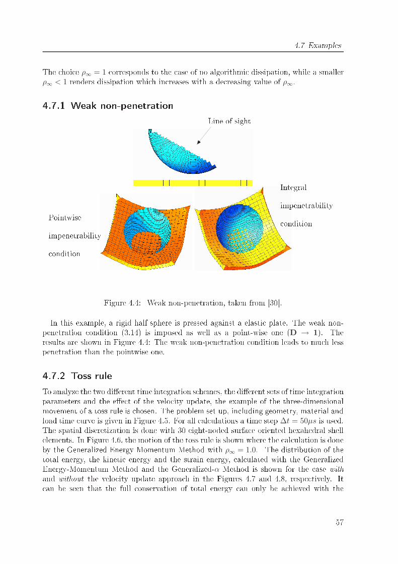
4.7 ExamplesThe hoi e ρ∞ = 1 orresponds to the ase of no algorithmi dissipation, while a smallerρ∞ < 1 renders dissipation whi h in reases with a de reasing value of ρ∞.4.7.1 Weak non-penetration Line of sightPointwiseimpenetrability ondition

Integralimpenetrability onditionFigure 4.4: Weak non-penetration, taken from [30.In this example, a rigid half sphere is pressed against a elasti plate. The weak non-penetration ondition (3.14) is imposed as well as a point-wise one (D → 1). Theresults are shown in Figure 4.4: The weak non-penetration ondition leads to mu h lesspenetration than the pointwise one.4.7.2 Toss ruleTo analyze the two dierent time integration s hemes, the dierent sets of time integrationparameters and the ee t of the velo ity update, the example of the three-dimensionalmovement of a toss rule is hosen. The problem set up, in luding geometry, material andload time urve is given in Figure 4.5. For all al ulations a time step ∆t = 50µs is used.The spatial dis retization is done with 30 eight-noded surfa e oriented hexahedral shellelements. In Figure 4.6, the motion of the toss rule is shown where the al ulation is doneby the Generalized Energy-Momentum Method with ρ∞ = 1.0. The distribution of thetotal energy, the kineti energy and the strain energy, al ulated with the GeneralizedEnergy-Momentum Method and the Generalized-α Method is shown for the ase withand without the velo ity update approa h in the Figures 4.7 and 4.8, respe tively. It an be seen that the full onservation of total energy an only be a hieved with the57

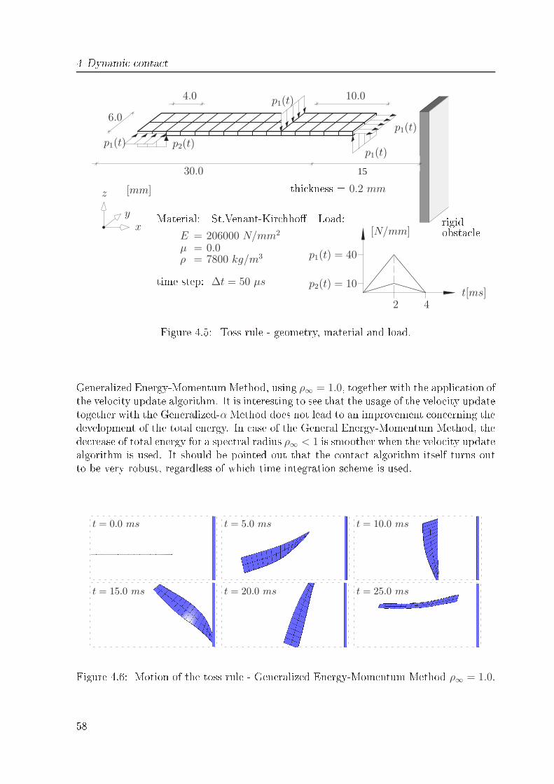
4 Dynami onta t15

PSfrag repla ements

6.0

4.0 10.0

30.0

[mm]

p1(t)

p1(t)p1(t)

p1(t)

p2(t)

xy

z thi kness = 0.2 mmMaterial: St.Venant-Kir hhoE 206000 N/mm2

µ 0.0ρ 7800 kg/m3=

==time step: ∆t = 50 µs

Load:p1(t) = 40

p2(t) = 10

[N/mm]

t[ms]2 4

rigidobsta leFigure 4.5: Toss rule - geometry, material and load.Generalized Energy-MomentumMethod, using ρ∞ = 1.0, together with the appli ation ofthe velo ity update algorithm. It is interesting to see that the usage of the velo ity updatetogether with the Generalized-αMethod does not lead to an improvement on erning thedevelopment of the total energy. In ase of the General Energy-Momentum Method, thede rease of total energy for a spe tral radius ρ∞ < 1 is smoother when the velo ity updatealgorithm is used. It should be pointed out that the onta t algorithm itself turns outto be very robust, regardless of whi h time integration s heme is used.

PSfrag repla ements t = 0.0 ms t = 5.0 ms t = 10.0 ms

t = 15.0 ms t = 20.0 ms t = 25.0 ms

Figure 4.6: Motion of the toss rule - Generalized Energy-Momentum Method ρ∞ = 1.0.58

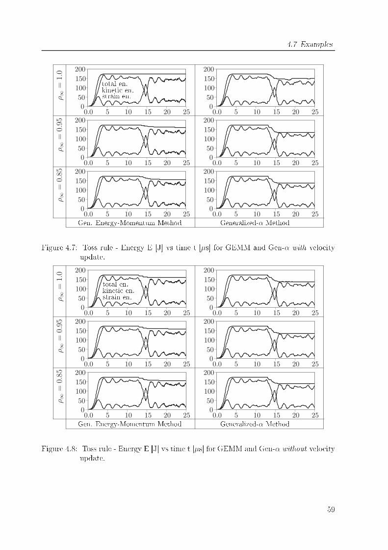
4.7 ExamplesPSfrag repla ements0.0

0.0

0.0 0.0

0.0

0.05

5

5 5

5

510

10

10 10

10

1015

15

15 15

15

1520

20

20 20

20

2025

25

25 25

25

250

0

0 0

0

0

50

50

50 50

50

50

100

100

100 100

100

100

150

150

150 150

150

150

200

200

200 200

200

200

Gen. Energy-Momentum Method Generalized-α Method

ρ∞

=1.

0ρ∞

=0.

95ρ∞

=0.

85

total en.kineti en.strain en.

Figure 4.7: Toss rule - Energy E [J vs time t [µs for GEMM and Gen-α with velo ityupdate.PSfrag repla ements0.0

0.0

0.0 0.0

0.0

0.05

5

5 5

5

510

10

10 10

10

1015

15

15 15

15

1520

20

20 20

20

2025

25

25 25

25

250

0

0 0

0

0

50

50

50 50

50

50

100

100

100 100

100

100

150

150

150 150

150

150

200

200

200 200

200

200

Gen. Energy-Momentum Method Generalized-α Method

ρ∞

=1.

0ρ∞

=0.

95ρ∞

=0.

85

total en.kineti en.strain en.

Figure 4.8: Toss rule - Energy E [J vs time t [µs for GEMM and Gen-α without velo ityupdate.59

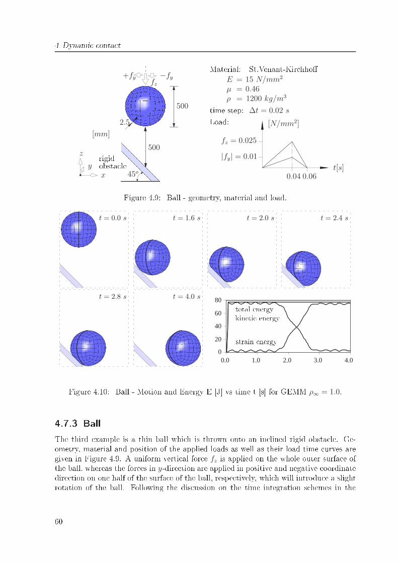
4 Dynami onta t

PSfrag repla ements

−fy+fyfz

Material: St.Venant-Kir hhoE 15 N/mm2

µ 0.46ρ 1200 kg/m3=

==time step: ∆t = 0.02 sLoad:

500

500

2.5

45o

[mm]

xy

z rigidobsta le fz = 0.025

|fy| = 0.01

0.04 0.06

[N/mm2]

t[s]Figure 4.9: Ball - geometry, material and load.

0.0 1.0 2.0 3.0 4.0

20

40

60

80

0

PSfrag repla ements t = 0.0 s t = 1.6 s t = 2.0 s t = 2.4 s

t = 2.8 s t = 4.0 s total energykineti energystrain energyFigure 4.10: Ball - Motion and Energy E [J vs time t [s for GEMM ρ∞ = 1.0.4.7.3 BallThe third example is a thin ball whi h is thrown onto an in lined rigid obsta le. Ge-ometry, material and position of the applied loads as well as their load time urves aregiven in Figure 4.9. A uniform verti al for e fz is applied on the whole outer surfa e ofthe ball, whereas the for es in y-dire tion are applied in positive and negative oordinatedire tion on one half of the surfa e of the ball, respe tively, whi h will introdu e a slightrotation of the ball. Following the dis ussion on the time integration s hemes in the60

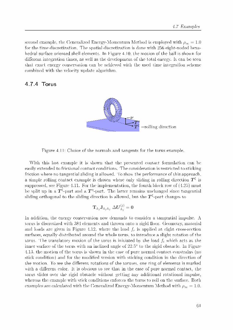
4.7 Examplesse ond example, the Generalized Energy-Momentum Method is employed with ρ∞ = 1.0for the time dis retization. The spatial dis retization is done with 256 eight-noded hexa-hedral surfa e oriented shell elements. In Figure 4.10, the motion of the ball is shown fordierent integration times, as well as the development of the total energy. It an be seenthat exa t energy onservation an be a hieved with the used time integration s heme ombined with the velo ity update algorithm.4.7.4 TorusT ξ =rolling dire tionT η

−ν

Figure 4.11: Choi e of the normals and tangents for the torus example.With this last example it is shown that the presented onta t formulation an beeasily extended to fri tional onta t onditions. The onsideration is restri ted to sti kingfri tion where no tangential sliding is allowed. To show the performan e of this approa h,a simple rolling onta t example is hosen where only sliding in rolling dire tion T ξ issuppressed, see Figure 4.11. For the implementation, the fourth blo k row of (4.25) mustbe split up in a T ξ-part and a T η-part. The latter remains un hanged sin e tangentialsliding orthogonal to the sliding dire tion is allowed, but the T ξ-part hanges toTAj

JAjAj∆U

(j)Aj

= 0In addition, the energy onservation now demands to onsider a tangential impulse. Atorus is dis retized with 384 elements and thrown onto a rigid oor. Geometry, materialand loads are given in Figure 4.12, where the load fr is applied at eight ross-se tionsurfa es, equally distributed around the whole torus, to introdu e a slight rotation of thetorus. The translatory motion of the torus is initiated by the load ft whi h a ts at theinner surfa e of the torus with an in lined angle of 22.5o to the rigid obsta le. In Figure4.13, the motion of the torus is shown in the ase of pure normal onta t onstrains (nosti k ondition) and for the modied version with sti king ondition in the dire tion ofthe motion. To see the dierent rotations of the toruses, one ring of elements is markedwith a dierent olor. It is obvious to see that in the ase of pure normal onta t, thetorus slides over the rigid obsta le without getting any additional rotational impulse,whereas the example with sti k onditions enfor es the torus to roll on the surfa e. Bothexamples are al ulated with the Generalized Energy-Momentum Method with ρ∞ = 1.0.61

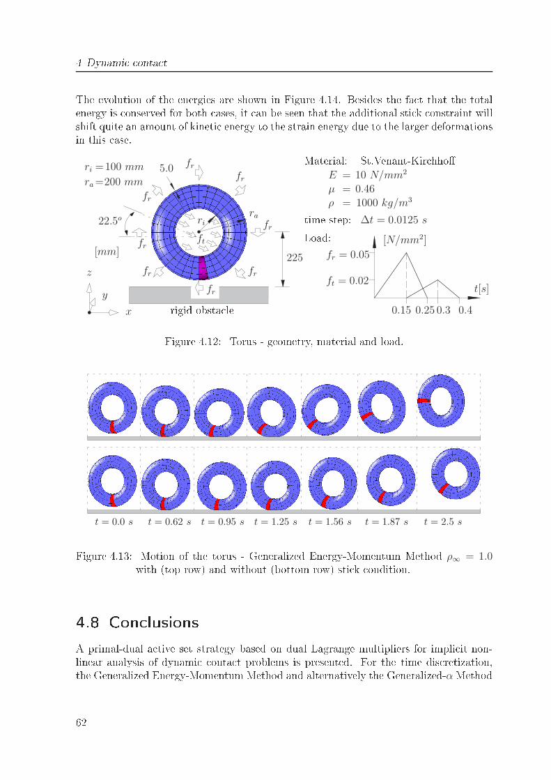
4 Dynami onta tThe evolution of the energies are shown in Figure 4.14. Besides the fa t that the totalenergy is onserved for both ases, it an be seen that the additional sti k onstraint willshift quite an amount of kineti energy to the strain energy due to the larger deformationsin this ase.

PSfrag repla ements

ft

fr

fr

fr

fr

fr

fr

fr

fr

Material: St.Venant-Kir hhoE 10 N/mm2

µ 0.46

ρ 1000 kg/m3=

==

==time step: ∆t = 0.0125 sLoad:

225

100 mm

200 mm5.0ri

ri

ra

ra

[mm]

x

y

z rigid obsta le ft = 0.02

fr = 0.05

0.15 0.25 0.3 0.4

[N/mm2]

t[s]

22.5o

Figure 4.12: Torus - geometry, material and load.PSfrag repla ements

t = 0.0 s t = 0.62 s t = 0.95 s t = 1.25 s t = 1.56 s t = 1.87 s t = 2.5 sFigure 4.13: Motion of the torus - Generalized Energy-Momentum Method ρ∞ = 1.0with (top row) and without (bottom row) sti k ondition.4.8 Con lusionsA primal-dual a tive set strategy based on dual Lagrange multipliers for impli it non-linear analysis of dynami onta t problems is presented. For the time dis retization,the Generalized Energy-Momentum Method and alternatively the Generalized-αMethod62

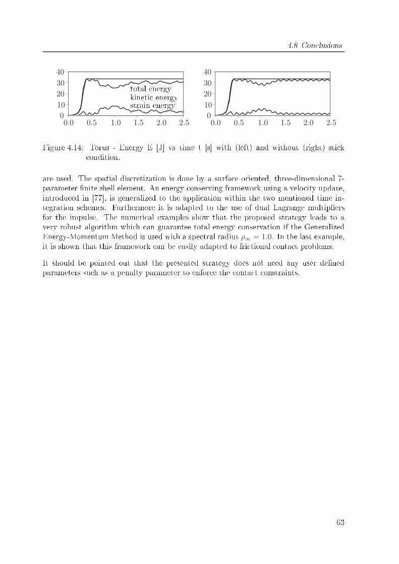
4.8 Con lusionsPSfrag repla ements

0.00.0 0.50.5 1.01.0 1.51.5 2.02.0 2.52.500

1010

2020

3030

4040 total energykineti energystrain energyFigure 4.14: Torus - Energy E [J vs time t [s with (left) and without (right) sti k ondition.are used. The spatial dis retization is done by a surfa e oriented, three-dimensional 7-parameter nite shell element. An energy onserving framework using a velo ity update,introdu ed in [77, is generalized to the appli ation within the two mentioned time in-tegration s hemes. Furthermore it is adapted to the use of dual Lagrange multipliersfor the impulse. The numeri al examples show that the proposed strategy leads to avery robust algorithm whi h an guarantee total energy onservation if the GeneralizedEnergy-Momentum Method is used with a spe tral radius ρ∞ = 1.0. In the last example,it is shown that this framework an be easily adapted to fri tional onta t problems.It should be pointed out that the presented strategy does not need any user denedparameters su h as a penalty parameter to enfor e the onta t onstraints.

63

5 Velo ity based onta t problemsThe aim of this hapter is to show the appli ability of the pdASeS to velo ity drivenproblems. The method is applied to the ring rolling of external spur gears, whi h is a rigid-plasti metal forming simulation. The existing displa ement based onta t formulationis adapted to a velo ity based one. A numeri al example is presented. The problemis restri ted again to the ase without inertia for es. Let ϕ be the urrent, unknowndeformation and dene the Almansi strain E byE :=

1

2

(

∇ϕ(x0)(u)⊤ +∇ϕ(x0)(u)−∇ϕ(x0)(u)⊤∇ϕ(x0)(u))Here is only important that E is a strain measure whi h is suited for the large deformation

ϕ, the workpie e is undergoing. The body Ω gets into onta t with a rigid obsta le Ωobswhi h has the boundary Γobs. By µplas, the vis osity oe ient for the plasti ow isdenoted and the bulk modulus κplas a ts as a volume penalty whi h is usually set to avery high value to nearly guarantee the plasti in ompressibilitytr(E)→ 0By p := −1

dtr(σ), the pressure is denoted, and s := σ + p1 is the deviatori stress.A ording to this, the onstitutive law [4 formulated in the a tual Cau hy stresses readsas

s = 2µplas dev(E), p = κplas tr(E)Sin e the material law is velo ity-driven, the Diri hlet boundary ondition has to be givenfor the velo ity u. The bivariate form of the internal energy isf rp(u,v) :=

∫

ϕ(Ω)

σ(u) : E(v)Sin e the stru tural term f rp(·, ·) is velo ity-driven, whereas the onta t onditions aredispla ement-driven, one has to express (3.15) in terms of the velo ity un+1. Therefore,a generalized trapezoidal rule is used with the parameter γ ∈ [0, 1]

∆un+1 = un+1 − un = (1− γ) ∆t un + γ ∆t un+1 (5.1)The di ulty of the large deformations is ta kled in an updated Lagrange manner. Thus,the gap g and the onta t normal ν are hosen with respe t to the last known ongu-ration at time tn. This means that g(xn, tn+1) is the distan e between the position xnat time tn and its losest point proje tion onto Γobs(tn+1). By ν(xn, tn+1), the dire tion65

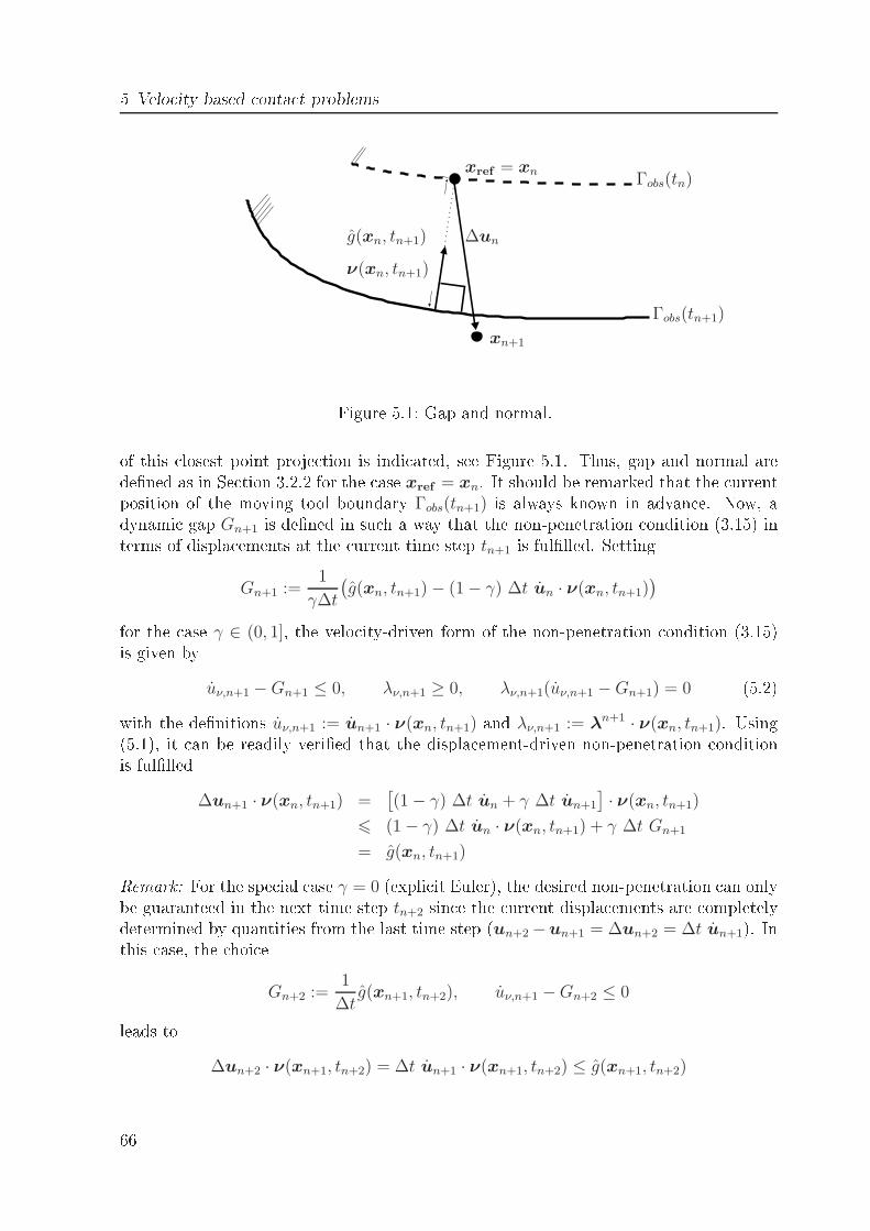
5 Velo ity based onta t problemsΓobs(tn+1)

Γobs(tn)xref = xn

xn+1

g(xn, tn+1)

ν(xn, tn+1)

∆un

Figure 5.1: Gap and normal.of this losest point proje tion is indi ated, see Figure 5.1. Thus, gap and normal aredened as in Se tion 3.2.2 for the ase xref = xn. It should be remarked that the urrentposition of the moving tool boundary Γobs(tn+1) is always known in advan e. Now, adynami gap Gn+1 is dened in su h a way that the non-penetration ondition (3.15) interms of displa ements at the urrent time step tn+1 is fullled. SettingGn+1 :=

1

γ∆t

(

g(xn, tn+1)− (1− γ) ∆t un · ν(xn, tn+1))for the ase γ ∈ (0, 1], the velo ity-driven form of the non-penetration ondition (3.15)is given by

uν,n+1 −Gn+1 ≤ 0, λν,n+1 ≥ 0, λν,n+1(uν,n+1 −Gn+1) = 0 (5.2)with the denitions uν,n+1 := un+1 · ν(xn, tn+1) and λν,n+1 := λn+1 · ν(xn, tn+1). Using(5.1), it an be readily veried that the displa ement-driven non-penetration onditionis fullled∆un+1 · ν(xn, tn+1) =

[

(1− γ) ∆t un + γ ∆t un+1

]

· ν(xn, tn+1)

6 (1− γ) ∆t un · ν(xn, tn+1) + γ ∆t Gn+1

= g(xn, tn+1)Remark: For the spe ial ase γ = 0 (expli it Euler), the desired non-penetration an onlybe guaranteed in the next time step tn+2 sin e the urrent displa ements are ompletelydetermined by quantities from the last time step (un+2−un+1 = ∆un+2 = ∆t un+1). Inthis ase, the hoi eGn+2 :=

1

∆tg(xn+1, tn+2), uν,n+1 −Gn+2 ≤ 0leads to

∆un+2 · ν(xn+1, tn+2) = ∆t un+1 · ν(xn+1, tn+2) ≤ g(xn+1, tn+2)66

As only the fri tionless ase is onsidered, the LM one M+ is given by (W is the tra espa e of [H10 ]d restri ted to the potential onta t boundary, M is its dual spa e)

M+ := µ ∈M : 〈µ,η〉 ≤ 0, η ∈W with ην ≤ 0The time dis retized variational formulation for the time step tn+1 reads as follows: nd

(un+1,λn+1) ∈ [H10 ]d ×M+ su h that

f rp(un+1,v) + 〈v,λn+1〉 = 0, v ∈ [H10 ]d

〈uν,n+1, µν − λν,n+1〉 ≤ 〈Gn+1, µν − λν,n+1〉, µ ∈M+(5.3)Let Krp be the rigid plasti stiness matrix resulting from the bivariate form f rp(·, ·)after dis retization in spa e and onsistent linearization of the geometri nonlinearity.Then, in analogy to (3.22), the algebrai form of (5.3) is given by

KrpUn+1 +

[

0

D

]

Λn+1 = 0together with the onta t onditionsUn+1

pν −Gn+1p ≤ 0, Λn+1

pν ≥ 0, (Un+1pν −Gn+1

p )Λn+1pν = 0, Λn+1

pτ = 0Along with the denition Nn+1p := ν(xn

p , tn+1), the abbreviationsUn+1

pν := Un+1

p ·Nn+1p , Λn+1

pν := Λn+1p ·Nn+1

p , Λn+1pτ := Λn+1

p − Λn+1pν Nn+1

pwere used. As a numeri al example, an in remental metal forming pro ess is onsidered,see the left upper pi ture in Figure 5.2. One mobile tool presses the material into arigid mold and forms a spur gear within 6000 time steps. The simulation was done inLARSTRAN. In Figures 5.2 and 5.3, one an see some snapshots out of the simulationpro ess. The movement of the mobile inner tool is not plotted, but at the rigid outertool, one an re ognize that the method is performing well.

67

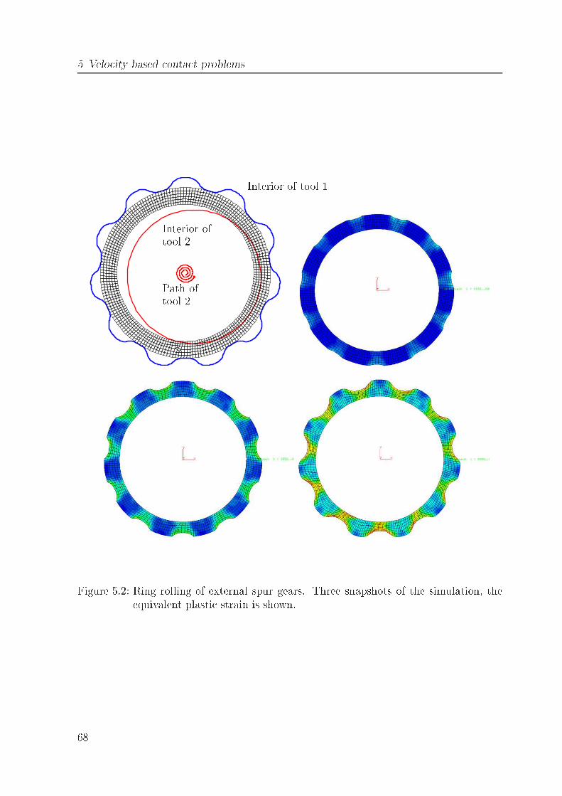
5 Velo ity based onta t problems

Interior oftool 2 Interior of tool 1Path oftool 2

Figure 5.2: Ring rolling of external spur gears. Three snapshots of the simulation, theequivalent plasti strain is shown.68

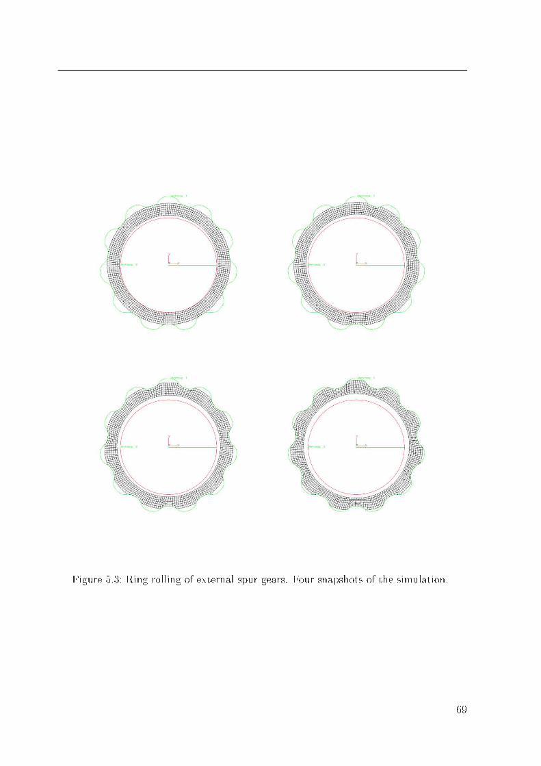
Figure 5.3: Ring rolling of external spur gears. Four snapshots of the simulation.69

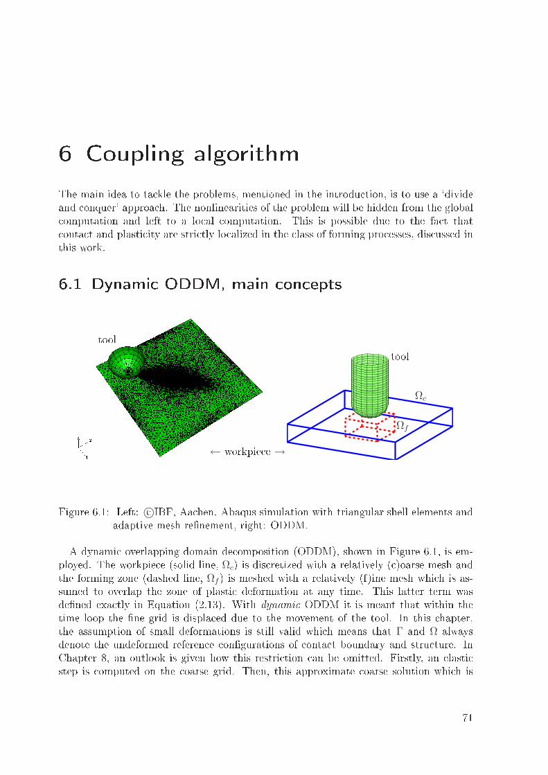
6 Coupling algorithmThe main idea to ta kle the problems, mentioned in the introdu tion, is to use a `divideand onquer' approa h. The nonlinearities of the problem will be hidden from the global omputation and left to a lo al omputation. This is possible due to the fa t that onta t and plasti ity are stri tly lo alized in the lass of forming pro esses, dis ussed inthis work.6.1 Dynami ODDM, main on eptstool

Ωc

Ωf

tool← workpie e →

Figure 6.1: Left: ©IBF, Aa hen, Abaqus simulation with triangular shell elements andadaptive mesh renement, right: ODDM.A dynami overlapping domain de omposition (ODDM), shown in Figure 6.1, is em-ployed. The workpie e (solid line, Ωc) is dis retized with a relatively ( )oarse mesh andthe forming zone (dashed line, Ωf ) is meshed with a relatively (f)ine mesh whi h is as-sumed to overlap the zone of plasti deformation at any time. This latter term wasdened exa tly in Equation (2.13). With dynami ODDM it is meant that within thetime loop the ne grid is displa ed due to the movement of the tool. In this hapter,the assumption of small deformations is still valid whi h means that Γ and Ω alwaysdenote the undeformed referen e ongurations of onta t boundary and stru ture. InChapter 8, an outlook is given how this restri tion an be omitted. Firstly, an elasti step is omputed on the oarse grid. Then, this approximate oarse solution whi h is71

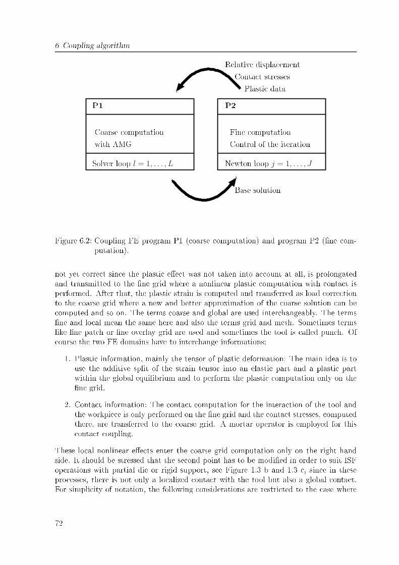
6 Coupling algorithmP1Coarse omputationwith AMGSolver loop l = 1, . . . , L Base solution

Relative displa ementConta t stressesPlasti dataP2Fine omputationControl of the iterationNewton loop j = 1, . . . , J

Figure 6.2: Coupling FE program P1 ( oarse omputation) and program P2 (ne om-putation).not yet orre t sin e the plasti ee t was not taken into a ount at all, is prolongatedand transmitted to the ne grid where a nonlinear plasti omputation with onta t isperformed. After that, the plasti strain is omputed and transferred as load orre tionto the oarse grid where a new and better approximation of the oarse solution an be omputed and so on. The terms oarse and global are used inter hangeably. The termsne and lo al mean the same here and also the terms grid and mesh. Sometimes termslike ne pat h or ne overlay grid are used and sometimes the tool is alled pun h. Of ourse the two FE domains have to inter hange informations:1. Plasti information, mainly the tensor of plasti deformation: The main idea is touse the additive split of the strain tensor into an elasti part and a plasti partwithin the global equilibrium and to perform the plasti omputation only on thene grid.2. Conta t information: The onta t omputation for the intera tion of the tool andthe workpie e is only performed on the ne grid and the onta t stresses, omputedthere, are transferred to the oarse grid. A mortar operator is employed for this onta t oupling.These lo al nonlinear ee ts enter the oarse grid omputation only on the right handside. It should be stressed that the se ond point has to be modied in order to suit ISFoperations with partial die or rigid support, see Figure 1.3 b and 1.3 , sin e in thesepro esses, there is not only a lo alized onta t with the tool but also a global onta t.For simpli ity of notation, the following onsiderations are restri ted to the ase where72

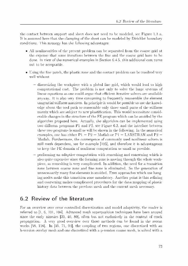
6.2 Review of the literaturethe onta t between support and sheet does not need to be modeled, see Figure 1.3 a.It is assumed here that the lamping of the sheet an be modeled by Diri hlet boundary onditions. This strategy has the following advantages:• All nonlinearities of the present problem an be separated from the oarse grid atthe expense that some iterations between the ne and the oarse grid have to bedone. In view of the numeri al examples in Se tion 6.4.5, this additional ost turnsout to be a eptable.• Using the ne pat h, the plasti zone and the onta t problem an be resolved verywell without dis retizing the workpie e with a global ne grid, whi h would lead to high omputational ost. The problem is not only to solve the large systems oflinear equations as one ould argue that e ient iterative solvers are availableanyway. It is also very time onsuming to frequently reassemble the elementtangential stiness matri es. In prin iple it would be possible to use the knowl-edge about the tool path to reassemble only those small parts of the stinessmatrix whi h are subje t to new plasti ation. This would ne essitate onsid-erable hanges in the stru ture of the FE program whi h an be avoided by thealgorithm proposed here. A tually, the algorithm an be implemented usingtwo dierent programs P1 and P2, see Figure 6.2, and the interfa e betweenthese two programs is small as will be shown in the following. In the numeri alexamples, one has either P1 = P2 = Matlab or P1 = LARSTRAN and P2 =Matlab. Furthermore, the onvergen e of ommonly used nonlinear solvers isstill mesh dependent, see for example [105, and therefore it is advantageousto keep the FE domain of nonlinear omputation as small as possible. performing an adaptive omputation with remeshing and oarsening whi h isalso quite expensive sin e the forming zone is moving through the whole work-pie e, so remeshing is very ompli ated. In addition, the need for a transitionzone between oarse zone and ne zone is eliminated. So the generation ofunne essarily many ne elements is avoided. Even approa hes whi h use hang-ing nodes make this transition zone mandatory. Another point is that reningand oarsening makes ompli ated pro edures for the data mapping of plasti history data between the previous mesh and the urrent mesh ne essary.6.2 Review of the literatureFor an overview over error ontrolled dis retization and model adaptivity, the reader isreferred to [1, 6, 101, 104. Advan ed mesh superposition te hniques have been aroundsin e the early nineties [39, 40, 80, often but not ex lusively in the ontext of ra kpropagation. A very good overview over those methods an be found in the re entworks [58, 116. In [35, 71, 94, the oupling of two regions, one dis retized with anh-version overlay mesh and one dis retized with a p-version oarse mesh, is solved with a73

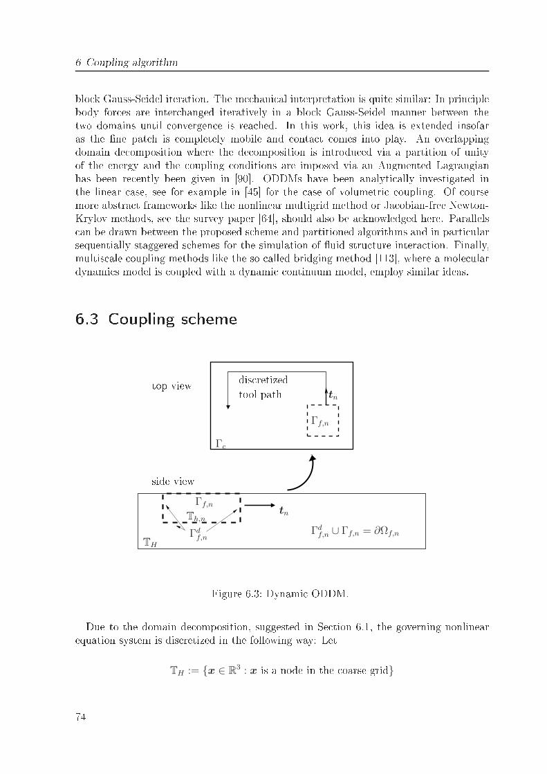
6 Coupling algorithmblo k Gauss-Seidel iteration. The me hani al interpretation is quite similar: In prin iplebody for es are inter hanged iteratively in a blo k Gauss-Seidel manner between thetwo domains until onvergen e is rea hed. In this work, this idea is extended insofaras the ne pat h is ompletely mobile and onta t omes into play. An overlappingdomain de omposition where the de omposition is introdu ed via a partition of unityof the energy and the oupling onditions are imposed via an Augmented Lagrangianhas been re ently been given in [90. ODDMs have been analyti ally investigated inthe linear ase, see for example in [45 for the ase of volumetri oupling. Of oursemore abstra t frameworks like the nonlinear multigrid method or Ja obian-free Newton-Krylov methods, see the survey paper [64, should also be a knowledged here. Parallels an be drawn between the proposed s heme and partitioned algorithms and in parti ularsequentially staggered s hemes for the simulation of uid-stru ture-intera tion. Finally,multis ale oupling methods like the so alled bridging method [113, where a mole ulardynami s model is oupled with a dynami ontinuum model, employ similar ideas.6.3 Coupling s heme

Th,n

TH

tn

Γdf,n

Γf,n

Γdf,n ∪ Γf,n = ∂Ωf,n

top viewΓf,n

tn

dis retizedtool pathΓcside viewFigure 6.3: Dynami ODDM.Due to the domain de omposition, suggested in Se tion 6.1, the governing nonlinearequation system is dis retized in the following way: Let

TH := x ∈ R3 : x is a node in the oarse grid74

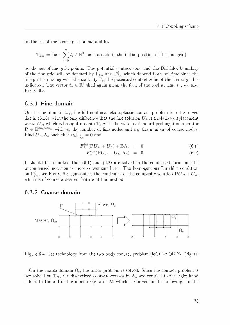
6.3 Coupling s hemebe the set of the oarse grid points and letTh,n := x+

n∑

i=0

ti ∈ R3 : x is a node in the initial position of the ne gridbe the set of ne grid points. The potential onta t zone and the Diri hlet boundaryof the ne grid will be denoted by Γf,n and Γd

f,n whi h depend both on time sin e thene grid is moving with the tool. By Γc, the potential onta t zone of the oarse grid isindi ated. The ve tor tn ∈ R3 shall again mean the feed of the tool at time tn, see alsoFigure 6.3.6.3.1 Fine domainOn the ne domain Ωf , the full nonlinear elastoplasti onta t problem is to be solvedlike in (3.18), with the only dieren e that the ne solution Uh is a relative displa ementw.r.t. UH whi h is brought up onto Th with the aid of a standard prolongation operator

P ∈ R3nh×3nH with nh the number of ne nodes and nH the number of oarse nodes.Find U h,Λh su h that uh|Γdf,n

= 0 and:F int

h (PUH +Uh) + BΛh = 0 (6.1)F con

h (PUH +Uh,Λh) = 0 (6.2)It should be remarked that (6.1) and (6.2) are solved in the ondensed form but theun ondensed notation is more onvenient here. The homogeneous Diri hlet onditionon Γdf,n, see Figure 6.3, guarantees the ontinuity of the omposite solution PUH +Uh,whi h is of ourse a desired feature of the method.6.3.2 Coarse domain

PSfrag repla ements Slave, ΩsMaster, Ωm

Γ

PSfrag repla ementsΩc

ΩfSlave,Master,Figure 6.4: Use te hnology from the two body onta t problem (left) for ODDM (right).On the oarse domain Ωc, the linear problem is solved. Sin e the onta t problem isnot solved on TH , the dis retized onta t stresses in Λh are oupled to the right handside with the aid of the mortar operator M whi h is derived in the following: In the75

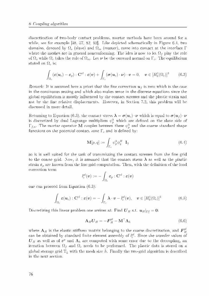
6 Coupling algorithmdis retization of two-body onta t problems, mortar methods have been around for awhile, see for example [38, 57, 82, 92. Like depi ted s hemati ally in Figure 6.4, twodomains, denoted by Ωs (slave) and Ωm (master), ome into onta t at the interfa e Γwhere the meshes are in general non onforming. The idea is now to let Ωf play the roleof Ωs while Ωc takes the role of Ωm. Let ν be the outward normal on Γc. The equilibriumstated on Ωc is:∫

Ωc

(ε(uc)− εp) : Cel : ε(v) +

∫

Γc

(σ(uc) · ν) · v = 0, v ∈ [H10 (Ωc)]

3 (6.3)Remark: It is assumed here a priori that the ne orre tion uf is zero whi h is the asein the ontinuous setting and whi h also makes sense in the dis rete equations sin e theglobal equilibrium is mostly inuen ed by the onta t stresses and the plasti strain andnot by the ne relative displa ements. However, in Se tion 7.2, this problem will bedis ussed in more detail.Returning to Equation (6.3), the onta t stress λ = σ(uc) ·ν whi h is equal to σ(uf) ·νis dis retized by dual Lagrange multipliers ψhp whi h are dened on the slave side of

Γf,n. The mortar operator M ouples between these ψhp and the oarse standard shapefun tions on the potential onta t zone Γc and is dened by:

M[p, q] :=

∫

Γc

ψhpφ

Hq I3 (6.4)so it is well suited for the task of transmitting the onta t stresses from the ne gridto the oarse grid. Now, it is assumed that the onta t stress λ as well as the plasti strain εp are known from the ne grid omputation. Then, with the denition of the load orre tion term

lplc (v) := −

∫

Ωc

εp : Cel : ε(v)one an pro eed from Equation (6.3):∫

Ωc

ε(uc) : Cel : ε(v) = −∫

Γc

λ · v − lplc (v), v ∈ [H1

0 (Ωc)]3 (6.5)Dis retizing this linear problem one arrives at: Find UH s.t. uH |Γd

c= 0:

AHUH = −F plH −M⊤Λh (6.6)where AH is the elasti stiness matrix belonging to the oarse dis retization, and F pl

H an be obtained by standard nite element assembly of lplc . Sin e the transfer values of

UH as well as of εp and Λh are omputed with some error due to the de oupling, aniteration between Ωf and Ωc needs to be performed. The plasti data is stored on aglobal storage grid Th with the mesh size h. Finally the two-grid algorithm is des ribedin the next se tion.76

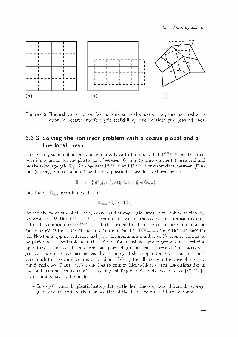
6.3 Coupling s heme

(a) (b) ( )Figure 6.5: Hierar hi al situation (a), non-hierar hi al situation (b), unstru tured situ-ation ( ), oarse interfa e grid (solid line), ne interfa e grid (dashed line).6.3.3 Solving the nonlinear problem with a oarse global and ane lo al meshFirst of all, some denitions and remarks have to be made: Let PGPS→C be the inter-polation operator for the plasti data between (G)auss (p)oints on the ( )oarse grid andon the (s)torage grid Th. Analogously PGPS→F and PGPF→S transfer data between (f)ineand (s)torage Gauss points. The dis rete plasti history data denes the setEh,n := [εp(ξ, tn), α(ξ, tn)] : ξ ∈ Gh,nand the set Eh,n a ordingly. Herein

Gh,n,GH and Ghdenote the positions of the ne, oarse and storage grid integration points at time tn,respe tively. With (·)(k), the kth iterate of (·) within the oarse-ne iteration is indi- ated. If a notation like (·)(•,⋆) is used, then • denotes the index of a oarse-ne iterationand ⋆ indi ates the index of the Newton iteration. Let TOLnewt denote the toleran e forthe Newton stopping riterion and jmax the maximum number of Newton iterations tobe performed. The implementation of the aforementioned prolongation and restri tionoperators in the ase of stru tured, axis-parallel grids is straightforward (`do-not-sear h-just- ompute'). As a onsequen e, the assembly of those operators does not ontributevery mu h to the overall omputation time. To keep the e ien y in the ase of unstru -tured grids, see Figure 6.5( ), one has to employ hierar hi al sear h algorithms like intwo body onta t problems with very large sliding or rigid body motions, see [87, 114.Two remarks have to be made:• In step 6, when the plasti history data of the last time step is read from the storagegrid, one has to take the new position of the displa ed ne grid into a ount. 77

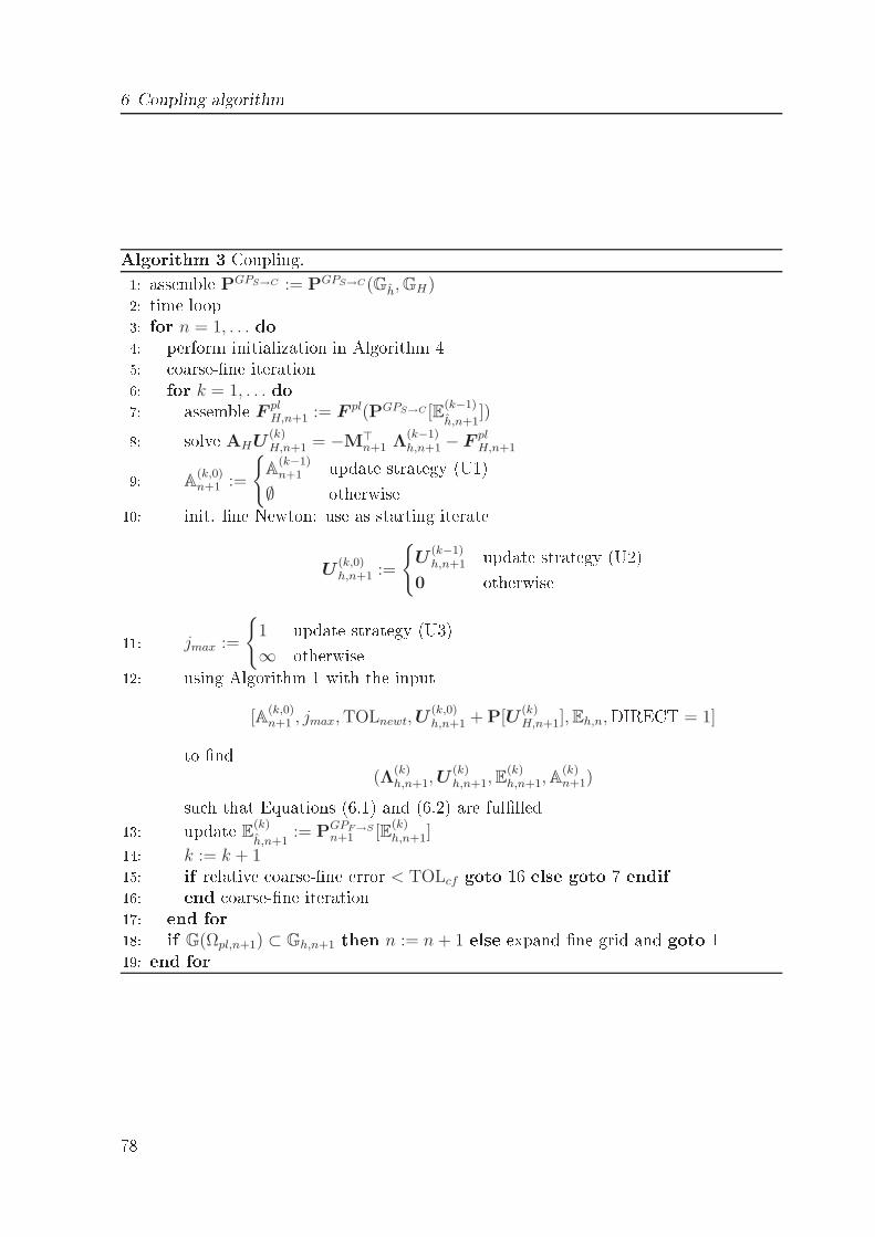
6 Coupling algorithmAlgorithm 3 Coupling.1: assemble PGPS→C := PGPS→C(Gh,GH)2: time loop3: for n = 1, . . . do4: perform initialization in Algorithm 45: oarse-ne iteration6: for k = 1, . . . do7: assemble F pl

H,n+1 := F pl(PGPS→C [E(k−1)

h,n+1])8: solve AHU

(k)H,n+1 = −M⊤

n+1 Λ(k−1)h,n+1 − F pl

H,n+19: A(k,0)n+1 :=

A(k−1)n+1 update strategy (U1)∅ otherwise10: init. ne Newton: use as starting iterate

U(k,0)h,n+1 :=

U(k−1)h,n+1 update strategy (U2)

0 otherwise11: jmax :=

1 update strategy (U3)∞ otherwise12: using Algorithm 1 with the input

[A(k,0)n+1 , jmax,TOLnewt,U

(k,0)h,n+1 + P[U

(k)H,n+1],Eh,n,DIRECT = 1]to nd

(Λ(k)h,n+1,U

(k)h,n+1,E

(k)h,n+1,A

(k)n+1)su h that Equations (6.1) and (6.2) are fullled13: update E

(k)

h,n+1:= P

GPF→S

n+1 [E(k)h,n+1]14: k := k + 115: if relative oarse-ne error < TOLcf goto 16 else goto 7 endif16: end oarse-ne iteration17: end for18: if G(Ωpl,n+1) ⊂ Gh,n+1 then n := n + 1 else expand ne grid and goto 119: end for

78

6.4 Numeri al resultsAlgorithm 4 Initialization.1: displa e ne grid Th,n+1 := Th,n + tn+12: assemble mortar operator Mn+1 := M(Th,n+1,TH)3: assemble Pn+1 := P(TH ,Th,n+1)4: assemble PGPF→S

n+1 := PGPF→S(Gh,n+1,Gh)5: assemble PGPS→F

n+1 := PGPS→F (Gh,Gh,n+1)6: read ne data from Gh : Eh,n := PGPS→F

n+1 [Eh,n]7: init. E(0)

h,n+1:= Eh,n, A

(0)n+1 := An, Λ

(0)h,n+1 := 0, U

(0)h,n+1 = 0

• Without going into details: In step 18, it is he ked whether plasti ation o urssomewhere outside the ne domain. In this ase, one has to distinguish betweentwo ases:1. The plasti zone is just a bit larger than assumed: Expand the ne domaina ordingly.2. New plasti ation o urred far outside the ne domain: The omputation hasto be stopped, sin e the intention of in remental forming pro esses is to haveplasti ation only in the forming zone, otherwise it is impossible to ontrolthese operations. In this ase, the tool path has to be re onsidered arefully.With the remark that a areful use of the update strategies (U1)-(U3) is ru ial to theperforman e of the algorithm, see the numeri al example in Part 6.4.5, this se tion is on luded.6.4 Numeri al resultsIn this se tion, some numeri al examples are presented to show the performan e of theproposed oupling methods.6.4.1 Material dataThe following set of material data is hosen for all the subsequent numeri al exam-ples: E = 69000, ν = 0.33. For the examples with elastoplasti material behavior,linear isotropi hardening is assumed with Y (α) = σ0 + Kα and with the additionalparameters K = 2538.930 and σ0 = 279.618. The pro ess ontrol parameters areTOLnewt = TOLcf = 10−8.6.4.2 Elasti example, non-hierar hi al aseIt will be demonstrated in this example that if one onsiders only the onta t problem andnot the material nonlinearity, the ne grid is able to move independently from the oarsegrid and does not ne essarily have to be a lo al renement of the global oarse grid. A79

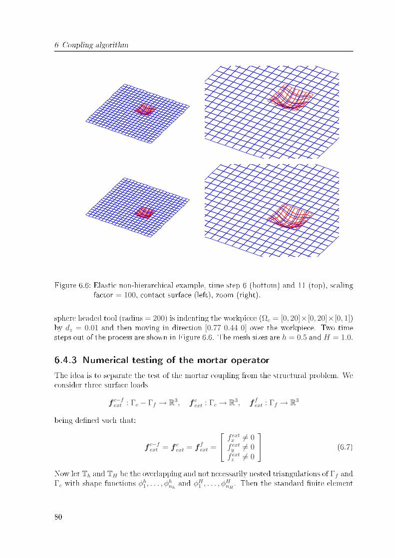
6 Coupling algorithm

Figure 6.6: Elasti non-hierar hi al example, time step 6 (bottom) and 11 (top), s alingfa tor = 100, onta t surfa e (left), zoom (right).sphere headed tool (radius = 200) is indenting the workpie e (Ωc = [0, 20]×[0, 20]×[0, 1])by dz = 0.01 and then moving in dire tion [0.77 0.44 0] over the workpie e. Two timesteps out of the pro ess are shown in Figure 6.6. The mesh sizes are h = 0.5 and H = 1.0.6.4.3 Numeri al testing of the mortar operatorThe idea is to separate the test of the mortar oupling from the stru tural problem. We onsider three surfa e loadsf

c−fext : Γc − Γf → R

3, f cext : Γc → R

3, ffext : Γf → R

3being dened su h that:f

c−fext = f c

ext = ffext =

f extx 6= 0f ext

y 6= 0f ext

z 6= 0

(6.7)Now let Th and TH be the overlapping and not ne essarily nested triangulations of Γf andΓc with shape fun tions φh

1 , . . . , φhnh

and φH1 , . . . , φ

HnH. Then the standard nite element80

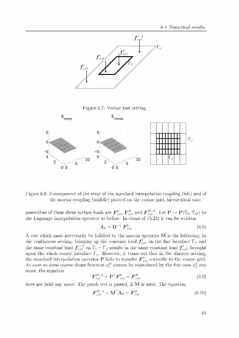
6.4 Numeri al resultsf c

ext

f cext

fc−fext

ffext

Γf

Γc

Figure 6.7: Mortar test setting.0

510

02

4−5

0

5

Einterp

05

10

02

4−5

0

5

Emortar

Γf

Γc

Figure 6.8: Z- omponent of the error of the standard interpolation oupling (left) and ofthe mortar oupling (middle) plotted on the oarse grid, hierar hi al ase.assemblies of these three surfa e loads are F hext,F

Hext and FH−h

ext . Let P := P(Th,TH) bethe Lagrange interpolation operator as before. In terms of (3.23) it an be written:Λh = D−1 F h

ext (6.8)A test whi h must ne essarily be fullled by the mortar operator M is the following: Inthe ontinuous setting, bringing up the onstant load f fext on the ne interfa e Γf andthe same onstant load f c−f

ext on Γc − Γf results in the same onstant load f cext, broughtupon the whole oarse interfa e Γc. However, it turns out that in the dis rete setting,the standard interpolation operator P fails to transfer F h

ext orre tly to the oarse grid.As soon as some oarse shape fun tion φHi annot be reprodu ed by the ne ones φh

j anymore, the equationFH−h

ext + P⊤F hext = FH

ext (6.9)does not hold any more. The pat h test is passed, if M is used: The equationFH−h

ext + M⊤Λh = FHext (6.10)81

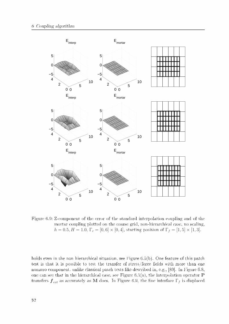
6 Coupling algorithm

05

10

02

4−5

0

5

Einterp

05

10

02

4−5

0

5

Emortar

05

10

02

4−5

0

5

Einterp

05

10

02

4−5

0

5

Emortar

05

10

02

4−5

0

5

Einterp

05

10

02

4−5

0

5

Emortar

Figure 6.9: Z- omponent of the error of the standard interpolation oupling and of themortar oupling plotted on the oarse grid, non-hierar hi al ase, no s aling,h = 0.5, H = 1.0, Γc = [0, 6]× [0, 4], starting position of Γf = [1, 5]× [1, 3].

holds even in the non-hierar hi al situation, see Figure 6.5(b). One feature of this pat htest is that it is possible to test the transfer of stress/for e elds with more than onenonzero omponent, unlike lassi al pat h tests like des ribed in, e.g., [89. In Figure 6.8,one an see that in the hierar hi al ase, see Figure 6.5(a), the interpolation operator Ptransfers f ext as a urately as M does. In Figure 6.9, the ne interfa e Γf is displa ed82

6.4 Numeri al resultsby the ve tor 0.05 d, 0.1 d and 0.2 d withd :=

[

0.770.4

]Even in this non-hierar hi al situation, the transfer error produ ed by M is zero whilethat stemming from P is in reasing. It is possible to pass this pat h test in the totallyunstru tured situation with methods introdu ed in [42. The onstant test load wasf ext = [20 37 100] in this example. In the left pi ture of Figure 6.9, the z- omponent ofthe error

Einterp := FH−hext + P⊤ F h

ext − FHextis plotted on the oarse grid of Γc, while in the middle, the z- omponent of the error

Emortar := FH−hext + M⊤ Λh − FH

ext (6.11)is displayed.Remark to the meaning of the pat h test Although the proof that Emortar = 0 isa dire t onsequen e of the theory of the mortar method, it is written down here in adire t form to explain what the pra ti al meaning of the mortar operator is. It turnsout that M is onstru ted in su h a way that it in orporates the information about thenon- onforming overlap between Γh and ΓH . The notations φir := φier and ψjr:= ψjerwith the unit ve tors er, r = 1, 2, 3 are introdu ed. Due to the test setting and (6.7), it an be stated that the following ontinuous equation is true:

fc−fext + f f

ext − f cext ≡ 0 ∈ R

3So for all i = 1, . . . , nh, r = 1, 2, 3 holds:∫

ΓH

fc−fext · φH

ir +

∫

ΓH

ffext · φH

ir −∫

ΓH

f cext ·φH

ir = 0

⇒∫

ΓH−Γh

fc−fext ·φH

ir +

∫

Γh

ffext · φH

ir −∫

ΓH

f cext ·φH

ir = 0The onstant for e density f fext an be reprodu ed by dual Lagrange multipliers ψjr

ffext =

∑

j∈Th,r=1,2,3

Λh[jr]ψhjr

(6.12)as well as the standard LMs whi h are identi al to the ne standard shape fun tions φjrin this setting:f

fext =

∑

j∈Th,r=1,2,3

F hext[jr]φ

hjr

(6.13)For example with the rst variant, one an pro eed:∫

ΓH−Γh

fc−fext · φH

ir +

∫

Γh

(

∑

j∈Th,r=1,2,3

Λh[jr]ψjr

)

· φHir −

∫

ΓH

f cext · φH

ir = 0

83

6 Coupling algorithmDue to the denitions, this is:FH−h

ext [ir] +∑

j∈Th,r=1,2,3

M⊤[ir, jr]Λh[jr]− FHext[ir] = 0 (6.14)For the omplete ve tors:

FH−hext + M⊤Λh − FH

ext = 0 (6.15)By omparing (6.12) and (6.13), one an easily see thatM⊤Λh = M⊤D−1F h

extNote that it is also possible to use the standard LMs for dis retizing f fext. Then the oupling operator is not M⊤ but M⊤D−1 sin e the oe ients in F h

ext are dierent fromthose in Λh. Only in the hierar hi al situation, the oupling operator M⊤D−1 equals thestandard pointwise interpolation operator P as one an easily derive using the Equations(3.10). By xhp , the oordinates of the p-th ne node are denoted.

M[p, q] =

∫

ΓH

ψhpφ

Hq 1

=

∫

ΓH

ψhp

(

4∑

k=1

φHq (xh

k)φhk

)

1

= φHq (xh

p)

∫

ΓH

φhp 1

= φHq (xh

p)D[p, p]

= P[p, q]D[p, p]With the operator P dened a ordingly:P[p, q] = φH

q (xhp)1 (6.16)6.4.4 Relative errorThis numeri al example onsiders the relative error of the two-grid solution w.r.t. aglobal ne one-grid solution. Four two-grid solutions, see Table 6.1, all with H = 1 and

h = 0.5, are ompared with the one-grid displa ement solution U ref with H = 0.5 forthe oarse domain Ωc = [0, 30]× [0, 10]× [0, 1]. In all four examples, only one time stepis omputed, elastoplasti material behavior is hosen, the geometry of the tool and theindention depth are the same as in Se tion 6.4.2. The relative error||U i −U ref ||∞||U ref ||∞

, i = 1, . . . , 4is shown in Figure 6.11. The expe ted behavior is that the relative error of a oarsegrid solution (0 nodes in the ne mesh) w.r.t the global ne solution an be already84

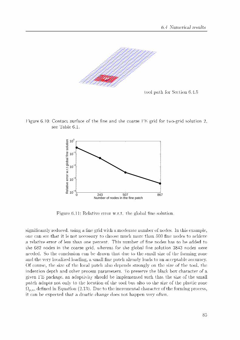
6.4 Numeri al results

tool path for Se tion 6.4.5Figure 6.10: Conta t surfa e of the ne and the oarse FE grid for two-grid solution 2,see Table 6.1.

0 243 507 86710

−4

10−3

10−2

10−1

100

Number of nodes in the fine patch

Rel

ativ

e er

ror

w.r

.t gl

obal

fine

sol

utio

n

Figure 6.11: Relative error w.r.t. the global ne solution.signi antly redu ed, using a ne grid with a moderate number of nodes. In this example,one an see that it is not ne essary to hoose mu h more than 500 ne nodes to a hievea relative error of less than one per ent. This number of ne nodes has to be added tothe 682 nodes in the oarse grid, whereas for the global ne solution 3843 nodes wereneeded. So the on lusion an be drawn that due to the small size of the forming zoneand the very lo alized loading, a small ne pat h already leads to an a eptable a ura y.Of ourse, the size of the lo al pat h also depends strongly on the size of the tool, theindention depth and other pro ess parameters. To preserve the bla k box hara ter of agiven FE pa kage, an adaptivity should be implemented su h that the size of the smallpat h adapts not only to the lo ation of the tool but also to the size of the plasti zoneΩp,n, dened in Equation (2.13). Due to the in remental hara ter of the forming pro ess,it an be expe ted that a drasti hange does not happen very often. 85

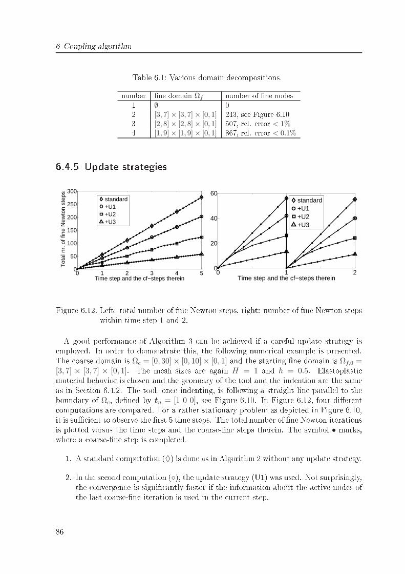
6 Coupling algorithmTable 6.1: Various domain de ompositions.number ne domain Ωf number of ne nodes1 ∅ 02 [3, 7] × [3, 7] × [0, 1] 243, see Figure 6.103 [2, 8] × [2, 8] × [0, 1] 507, rel. error < 1%4 [1, 9] × [1, 9] × [0, 1] 867, rel. error < 0.1%6.4.5 Update strategies

0 1 2 3 4 50

50

100

150

200

250

300

Time step and the cf−steps therein

Tot

al n

r. o

f fin

e N

ewto

n st

eps

standard+U1+U2+U3

0 1 20

20

40

60

Time step and the cf−steps therein

standard+U1+U2+U3

Figure 6.12: Left: total number of ne Newton steps, right: number of ne Newton stepswithin time step 1 and 2.A good performan e of Algorithm 3 an be a hieved if a areful update strategy isemployed. In order to demonstrate this, the following numeri al example is presented.The oarse domain is Ωc = [0, 30]× [0, 10]× [0, 1] and the starting ne domain is Ωf,0 =[3, 7] × [3, 7] × [0, 1]. The mesh sizes are again H = 1 and h = 0.5. Elastoplasti material behavior is hosen and the geometry of the tool and the indention are the sameas in Se tion 6.4.2. The tool, on e indenting, is following a straight line parallel to theboundary of Ωc, dened by tn = [1 0 0], see Figure 6.10. In Figure 6.12, four dierent omputations are ompared. For a rather stationary problem as depi ted in Figure 6.10,it is su ient to observe the rst 5 time steps. The total number of ne Newton iterationsis plotted versus the time steps and the oarse-ne steps therein. The symbol • marks,where a oarse-ne step is ompleted.1. A standard omputation (♦) is done as in Algorithm 2 without any update strategy.2. In the se ond omputation (), the update strategy (U1) was used. Not surprisingly,the onvergen e is signi antly faster if the information about the a tive nodes ofthe last oarse-ne iteration is used in the urrent step.86

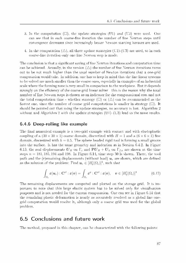
6.5 Con lusions and future work3. In the omputation (), the update strategies (U1) and (U2) were used. One an see that in ea h oarse-ne iteration the number of ne Newton steps until onvergen e de reases sin e in reasingly better Newton starting iterates are used.4. In the omputation (), all three update strategies (U1)-(U3) are used, so in ea h oarse-ne iteration only one ne Newton step is made.The on lusion is that a signi ant saving of ne Newton iterations and omputation time an be a hieved. A tually, in the version () the number of ne Newton iterations turnsout to be not mu h higher than the total number of Newton iterations that a one-grid omputation would take. In addition, one has to keep in mind that the ne linear systemsto be solved are mu h smaller than the oarse ones, espe ially in examples of an industrials ale where the forming zone is very small in omparison to the workpie e. But it dependsstrongly on the e ien y of the oarse grid linear solver - this is the reason why the totalnumber of ne Newton steps is hosen as an indi ator for the omputational ost and notthe total omputation time - whether strategy () or () an be re ommended as thefastest one, sin e the number of oarse grid omputations is smaller in strategy (). Itshould be pointed out that using the update strategies, no a ura y is lost. Algorithm 2without and Algorithm 2 with the update strategies (U1)(U3) lead to the same results.6.4.6 Deep-rolling like exampleThe nal numeri al example is a two-grid example with onta t and with elastoplasti oupling of a (30× 30× 1) oarse domain, dis retized with H = 1 and a (6× 6× 1) nedomain, dis retized with h = 0.5. The sphere headed rigid tool is forming a small grooveinto the surfa e. It has the same geometry and indention as in Se tion 6.4.2. In Figure6.13, the real displa ements UH on Γc and PUH + Uh on Γf,n are shown at the timesteps n = 181, 185, 194 and 198. In Figure 6.14, time step 30 is shown. There, the toolpath and the (r)emaining displa ements (without load) ur are shown, whi h are denedas the solution of the problem: Find ur ∈ [H10 (Ωc)]

3, su h that∫

Ωc

ε(ur) : Cel : ε(v) =

∫

Ωc

εp : Cel : ε(v), v ∈ [H10 (Ωc)]

3 (6.17)The remaining displa ements are omputed and plotted on the storage grid. It is im-portant to note that this large elasti system has to be solved only for visualizationpurposes and is not needed for the urrent omputation. One an see in Figure 6.14 thatthe remaining plasti deformation is nearly as a urately resolved as a global ne one-grid omputation would resolve it, although only a oarse grid was used for the globalproblem.6.5 Con lusions and future workThe method, proposed in this hapter, an be hara terized with the following points:87

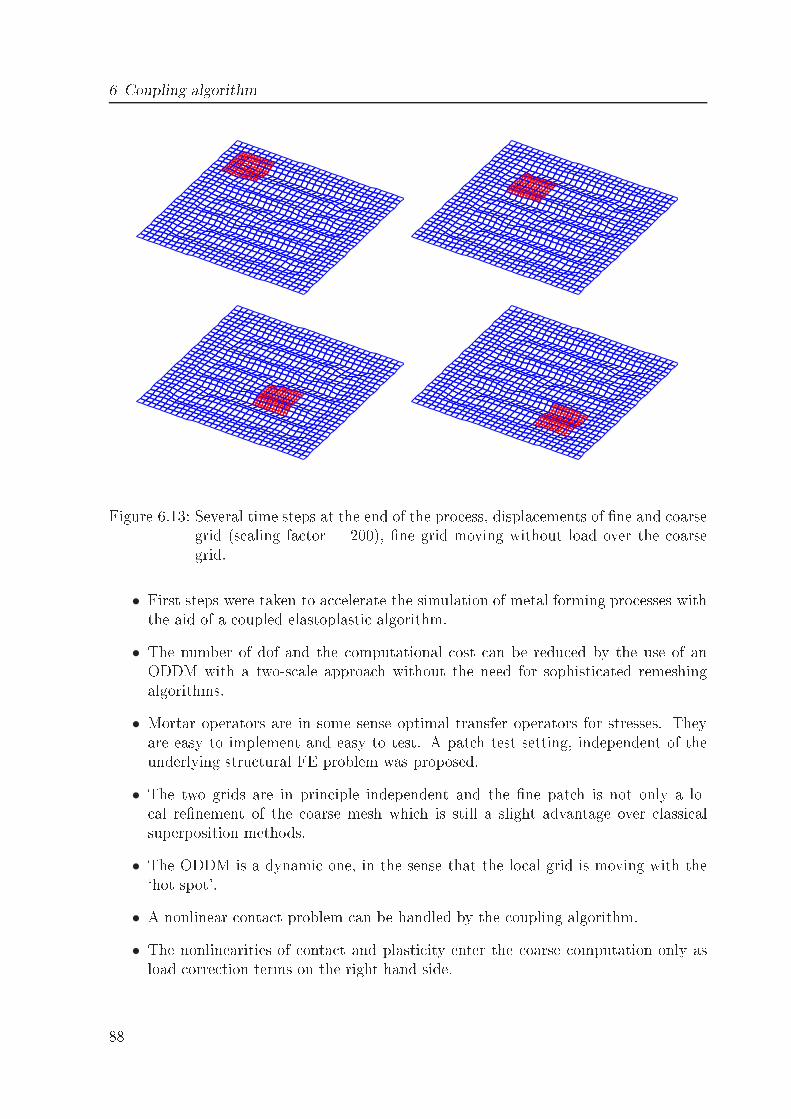
6 Coupling algorithm

Figure 6.13: Several time steps at the end of the pro ess, displa ements of ne and oarsegrid (s aling fa tor = 200), ne grid moving without load over the oarsegrid.• First steps were taken to a elerate the simulation of metal forming pro esses withthe aid of a oupled elastoplasti algorithm.• The number of dof and the omputational ost an be redu ed by the use of anODDM with a two-s ale approa h without the need for sophisti ated remeshingalgorithms.• Mortar operators are in some sense optimal transfer operators for stresses. Theyare easy to implement and easy to test. A pat h test setting, independent of theunderlying stru tural FE problem was proposed.• The two grids are in prin iple independent and the ne pat h is not only a lo- al renement of the oarse mesh whi h is still a slight advantage over lassi alsuperposition methods.• The ODDM is a dynami one, in the sense that the lo al grid is moving with the`hot spot'.• A nonlinear onta t problem an be handled by the oupling algorithm.• The nonlinearities of onta t and plasti ity enter the oarse omputation only asload orre tion terms on the right hand side.88

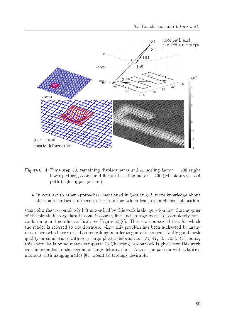
6.5 Con lusions and future work

510

1520

25

010

2030

−0.01

−0.005

0

zoomtool path andplotted time steps

plasti andelasti deformation

−3

−2

−1

0

1

2

3

4

5x 10

−330181184194198

Figure 6.14: Time step 30, remaining displa ements and α, s aling fa tor = 300 (rightlower pi ture), oarse and ne grid, s aling fa tor = 200 (left pi tures), toolpath (right upper pi ture).• In ontrast to other approa hes, mentioned in Se tion 6.2, more knowledge aboutthe nonlinearities is utilized in the iterations whi h leads to an e ient algorithm.One point that is ompletely left untou hed by this work is the question how the mappingof the plasti history data is done if oarse, ne and storage mesh are ompletely non- onforming and non-hierar hi al, see Figure 6.5( ). This is a non-trivial task for whi hthe reader is referred to the literature, sin e this problem has been addressed by manyresear hers who have worked on remeshing in order to guarantee a persistently good meshquality in simulations with very large plasti deformation [24, 47, 79, 103. Of ourse,this short list is by no means omplete. In Chapter 8, an outlook is given how this work an be extended to the regime of large deformations. Also a omparison with adaptivemethods with hanging nodes [85 would be strongly desirable.

89

7 An inexa t Newton blo k s hemeThe aim of this hapter is to review some algorithmi aspe ts of the oupling method inSe tion 6. For simpli ity, the notation is still restri ted to the regime of small deforma-tions.7.1 MotivationThe stru ture of Algorithm 3 was basi ally this one: oarse-neloop oarse linearsystemsystem solver loopne NewtonIn this se tion, also this stru ture is investigated:Newton oarse tangentialsystemsystem solver loopne tangential systemIt turns out that, organized in this manner, the numeri al s heme an be put mu h easierinto the perspe tive of more lassi al inexa t Newton s hemes. This is expe ted to makethe algorithm more reliable and easier to globalize in the sense that damping s hemesfrom the literature an be employed to guarantee global onvergen e. The questionswhi h arise are:• Is this method still e ient?• Is the algorithmi interfa e between oarse and ne still small?• Is it even possible to omit the oarse-ne iteration?7.2 Blo k iterative s heme: Linear elasti ityThe following dis rete FE spa es are introdu ed:

Vh ⊂ [H1(Ωf )]d, VH ⊂ [H1(Ωc)]

d, V0h ⊂ [H10 (Ωf)]

d, V0H ⊂ [H10 (Ωc)]

d 91

7 An inexa t Newton blo k s hemeThe subje t of publi ations like for instan e [45 is to solve multis ale ellipti problemson a lo ally enri hed spa e. Written in weak form: Find u ∈ V0h ⊕ V0H su h thata(u,v) =

∫

Ω

f ext · v, v ∈ V0h ⊕ V0HIn [45, the bilinear form a(·, ·) omes from the weak formulation of the Lapla e equa-tion, whereas here it stems from the weak formulation of the elasti ity equation. Afterdis retization one arrives at[

Ah AhH

AHh AH

] [

Uh

UH

]

=

[

Fext

h

Fext

H

] (7.1)with AhH the FE assembly of a(u,v) in VH × Vh and AHh the FE assembly of a(u,v)in Vh×VH . With the hat symbol is meant that the (zero) Diri hlet boundary onditionsare not yet in luded in this system, so, for exampleAh =

[

Ah Ah,NfDf

Ah,DfNfAh,DfDf

] and Uh =

[

Uh

0

]with Nf and Df denoting the free stru ture dof and the Diri hlet dof of the ne systemwith Nf ∩Df = ∅. After the removal of Diri hlet rows and olumns, the following redu edsystem is obtained:[

Ah AhH,NfNc

AHh,NcNfAH

] [

Uh

UH

]

=

[

F exth

F extH

] (7.2)In [45, the mixed matri es AhH and AHh are set up orre tly, whi h involves omput-ing the interse tions of elements of the dis retization of Vh and VH . After that, a Xutype su essive subspa e orre tion method is employed to solve this 2× 2 blo k systemiteratively. This way is not pursued entirely in this work:1. First of all, the oupling AHh is negle ted ompletely, sin e it is assumed that thene grid orre tion does not substantially inuen e the oarse grid solution apartfrom the onta t stresses and the plasti deformation history. A blo k iterativesolution of (7.2) is then not ne essary any more, be ause of the blo k triangularstru ture whi h saves a lot of omputation time. Another reason for these simpli- ations is to avoid algorithmi di ulties arising from the ne essity to guaranteethat the sum of Vh(tn) and VH is a dire t sum at any time tn, whi h is a ne essaryrequirement that the matrix in (7.2)lhs is invertible. Due to the movement of thetool, the spa e Vh(tn) depends on the position of the tool and therefore it anhappen very easily that the sum of the spa es is not dire t any more. Therefore,the assumption of a dire t sum is omitted.2. Se ondly, the oupling AhH is approximated by AhP with P from Equation (6.16),so the omputation of element interse tions is not ne essary any more, whi h isin parti ular in 3D advantageous, when it omes to the use of general hexahedralelements.92

7.3 Newton Blo k iterative s heme: Elasti ity with onta tWith this and the auxiliary omputationAhH,NfNc

UH = [AhP]NfNcUH = [AhPUH ]Nf

= Ah[PUH ]Nf+ Ah,NfDf

[PUH ]Df(7.3)(here it is assumed that P maps only the free oarse stru ture dof in Nc and not Dc tothe ne grid, so P ∈ RNf+Df×Nc), one ends up with the blo k iterative s heme

[

Ah [AhP]NfNc

0 AH

] [

Uh

UH

]

=

[

F exth

F extH

] (7.4)Thus, the fo us of this work is not a very high resolution of the underlying ellipti problem, but an e ient formulation whi h is able to hide the di ulties of onta t andplasti ity from the global domain. This will be explained in more detail in the followingse tions, where System (7.4) is extended by two blo k rows and blo k olumns to a ountfor onta t and material nonlinearity.7.3 Newton Blo k iterative s heme: Elasti ity with onta tDue to the reasons illustrated in Se tion 7.2 it is not attempted here, to start from aweak form over the lo ally enri hed spa e, although this would be desirable for analyti alreasons. The starting point here is rather a slightly simplied, full, dis rete, nonlinearproblem:F (Uh,Λh,UH) :=

[

F h

FH

]

:=

AhUh + [AhPUH ]Nf+ BΛh

F conh (Uh + PUH ,Λh)AHUH + M⊤Λh

!= 0Herein, Ah and AH are the elasti stinesses of Th and TH . Meaning of the three linesof the system:1. Fine equilibrium with the ne solution as orre tion of the oarse solution a ordingto the rst blo k row of (7.4) and with the onta t for es.2. Nonlinear omplementarity (NCP) fun tion.3. Coarse equilibrium a ording to the se ond blo k row of (7.4) with the load or-re tion due to onta t.Now, following Equations (3.16),(3.21) and (3.22), this nonlinear system an be onsis-tently linearized: With

K :=∂F

∂(U h,Λh,UH)the Ja obi matrixK =

[

Khh KhH

KHh KHH

]

=

Ah B [AhP]Nf•

Nh Th NhPNf•

0 M⊤ AH

(7.5)93

7 An inexa t Newton blo k s hemeis dened with the abbreviations:Nh :=

∂F conh

∂U=

0 0 0

0 0 −NA

0 0 0

, using the ordering U =

UN

UA

U I

Th :=∂F con

h

∂Λh

=

1 0

0 0

0 TA

, using the ordering Λh =

[

ΛI

ΛA

]

U := U(Uh,UH) := Uh + PUHFinally, in every Newton step j, the 2× 2 blo k system[

Khh KhH

KHh KHH

](j−1) [∆Xh

∆XH

](j)

= −[

F h

FH

](j−1) (7.6)has to be solved. Here, the following denitions were made:∆X

(j)h :=

[

∆U(j)h,N, ∆U

(j)h,Ij−1

, ∆U(j)h,Aj−1

, ∆Λ(j)h,Ij−1

, ∆Λ(j)h,Aj−1

]⊤

, ∆X(j)H := ∆U

(j)HThus, the domain de omposition into oarse and ne denes in a very natural way theblo k de omposition for the blo k iterative s heme, like des ribed in [96 and the refer-en es therein.7.4 Newton Blo k iterative s heme: Plasti ity with onta tIn this se tion, also the material nonlinearity is taken into a ount. The idea is tointrodu e an additional unknown up

f ∈ [H10 (Ωf )]

d as the Galerkin proje tion of the plasti strain in rement with respe t to the elasti ity bilinear form a(·, ·) (see also formula (6.17))∫

Ωf

ε(upf ) : Cel : ε(v) =

∫

Ωf

∆εpf,n+1 : Cel : ε(v), v ∈ V0hand to dene utr

f su h that uf an be split up additively into uf = utrf − up

f . This isa purely titious de omposition. In parti ular ∇symupf = ε

pf,n+1 − εp

f,n does not hold.Another problem is that the plasti dislo ations whi h are aptured by the in ompatible[72 strain eld εpf , are now smoothed out by this proje tion. In parti ular, also the eigenstrains are ontained in up

f . This is the reason why nally the upf will not be stored onthe storage grid but the plasti strain εp

f . With this, the overall nonlinear problem is:F (X) := F (Xh,XH) := F (U tr

h ,Λh,Uph,UH)

:=

[

F h(Utrh ,Λh,U

ph,UH)

FH(Λh,Uph,UH)

]

:=

Ah(Utrh −U p

h) + [AhPUH ]Nf+ BΛh + F pl

h,n

F conh (U tr

h + PUH ,Λh)

F inth (U tr

h + PUH)−Ah(Utrh −U p

h)− [AhPUH ]Nf− F pl

h,n

AHUH −P⊤Ah,•NfU

ph + M⊤Λh + F pl

H,n

!= 0 (7.7)

94

7.4 Newton Blo k iterative s heme: Plasti ity with onta twith F inth the standard nite element assembly of

∫

Ωf

σ(u) : ε(v), relation σ(u) fully nonlinear=

∫

Ωf

(ε(utrf + uc)− εp

f,n −∆εpf,n+1) : Cel : ε(v)and with F pl

h,n the standard nite element assembly oflplf := −

∫

Ωf

εpf,n : Cel : ε(v)The latter term is in luded in the rst and in the third blo k row of system (7.7) toa ount for the plasti deformation history until time step tn. The meaning of the fourlines of system (7.7) is:1. Fine equilibrium with the ne solution as orre tion of the oarse solution andwith the onta t for es. Under the assumption that up

f is known, this would be anequation for the nonlinear relation σ(u).2. NCP fun tion.3. This is again the spatial dis retization of the ne equilibrium. Now under theassumption that the nonlinear relation σ(u) is known, this would be an equationfor upf . In this blo k row, the plasti onstitutive law omes into play.4. Coarse equilibrium with the load orre tion terms due to onta t and plasti ity.With

K :=∂F

∂(U trh ,Λh,U

ph,UH)the Ja obi matrix is dened:

K =

[

Khh KhH

KHh KHH

]

=

Ah B −Ah [AhP]Nf•

Nh Th 0 NhPNf•

Kph 0 Ah [Kp

hP]Nf•

0 M⊤ −P⊤Ah,•NfAH

(7.8)Herein, Kp is dened as the FE assembly of−∫

Ωf

ε(u) : Cp : ε(v)with the fourth order tensor Cp dened in Equation (2.19).Remark: If one an els the third row and the third olumn of (7.8) (problem withoutplasti ity) one arrives again at (7.5). 95

7 An inexa t Newton blo k s heme7.5 Blo k iterative s hemesFor the solution of problem (7.6), several blo k iterative s hemes are appli able. Two ofthem are given here:Blo k-Ja obi: Fix j, for k = 1, . . . , K solveK

(j−1)hh ∆X

(j,k)h = −F (j−1)

h −K(j−1)hH ∆X

(j,k−1)H (7.9)

K(j−1)HH ∆X

(j,k)H = −F (j−1)

H −K(j−1)Hh ∆X

(j,k−1)h (7.10)In prin iple it is possible to parallelize (7.9), (7.10). But also the solving of the oarselinear system an be parallelized on its part.

K asesome value Kj inexa t Newton, see [37 and Se tion 7.71 Newton = oarse-ne iteration, in luded inAlgorithm 3 when update strategy (U3) isusednot xed iteration stops when onvergen e riterion ismetBlo k Gauss Seidel: Fix j, for k = 1, . . . , K solve

K(j−1)hh ∆X

(j,k)h = −F (j−1)

h −K(j−1)hH ∆X

(j,k−1)H (7.11)

K(j−1)HH ∆X

(j,k)H = −F (j−1)

H −K(j−1)Hh ∆X

(j,k)h (7.12)As before, (7.11) an be solved in the ondensed form (3.24).7.6 S hur omplement methodHaving a loser look at the Equations (7.11) and (7.12), one re ognizes that it is possibleto make the oarse-ne iteration obsolete at the expense that the appli ation of A−1

hon the matrix B has to be omputed. Furthermore, good onvergen e of the Newtoniteration annot be a hieved, as it will be shown.7.6.1 S hur omplement method, elasti aseEquation (7.11), written expli itly is[

Ah B(j−1)

N(j−1)h T

(j−1)h

] [

∆U h

∆Λh

](j,k)

= −[

F h,1

F h,2

](j−1)

−[

[AhP]Nf•

NhPNf•

](j−1)

∆U(j,k−1)H (7.13)96

7.6 S hur omplement methodUsing 1 a S hur omplement formula from standard textbooks like e.g. [96, the Newtonin rement of the onta t stresses an be omputed using Equation (7.3):(Th −NhA

−1h B)(j−1)∆Λ

(j,k)h

= −F (j−1)h,2 −N

(j−1)h PNf•∆U

(j,k−1)H + N

(j−1)h A−1

h F(j−1)h,1 + N

(j−1)h A−1

h [AhP∆U(j,k−1)H ]Nf

= −F (j−1)h,2 + N

(j−1)h A−1

h F(j−1)h,1 + F

(j,k−1)h,Df

(7.14)with the abbreviationF

(j,k−1)h,Df

:= N(j−1)h A−1

h Ah,NfDf[P∆U

(j,k−1)H ]DfThe matrix

Th −NhA−1h B (7.15)is nonsingular as long as the matrix in Equation (7.13)lhs is nonsingular, see page 457 of[96. Equation (7.14) reveals that, ex ept from

F(j,k−1)h,Dfall parts of the right hand side, ontaining ∆UH an be eliminated. Negle ting thisterm, the right hand does not depend on k any more whi h means that approximationsof ∆Λh,∆UH and ∆Uh an be omputed dire tly in this order:

(Th −NhA−1h B)(j−1)∆Λ

(j)

h = −F (j−1)h,2 + N

(j−1)h A−1

h F(j−1)h,1 (7.16)

AH∆U(j)

H = −AHU(j−1)

H −M⊤Λ(j−1)

h −M⊤∆Λ(j)

h (7.17)Ah∆U

(j)

h = −Ah(Uh + PUH)(j−1)

−B(Λ(j−1)

h + ∆Λ(j)

h )−AhP∆U(j)

H (7.18)For the Equations (7.17) and (7.18), the formulas (7.11) and (7.12) were just resolvedafter the desired variables. This an be simplied to:(Th −NhA

−1h B)(j−1)∆Λ

(j)

h = −F (j−1)h,2 + N

(j−1)h A−1

h F(j−1)h,1 (7.19)

AHU(j)

H = −M⊤Λ(j)

h (7.20)Ah∆U

(j)

h = −Ah(U(j−1)

h + PU(j)

H )−BΛ(j)

h (7.21)Negle ting the boundary term F(j,k−1)h,Df

will of ourse deteriorate the onvergen e of theNewton iteration signi antly, see Figure 7.2 in Se tion 7.9.3. Nevertheless, this method an be used to ompute a very good starting iterate for the inexa t Newton blo k GaussSeidel (GS) method, as des ribed in Se tion 7.7.1Idea from Dipl. Math. Corinna Hager, IANS, Stuttgart 97

7 An inexa t Newton blo k s heme7.6.2 S hur omplement method, plasti aseIn the plasti ase, Equation (7.11) is written expli itly with the aid of Equations (7.7)and (7.8),[

Ah Z1

Z2 Z3

](j−1) [∆U tr

h

∆Ξ

](j,k)

=

[

−F h,1

−F h,[2;3]

](j−1)

−[

[AhP]Nf•

Z2

]

∆U(j,k−1)H (7.22)with the abbreviations

Z1 := [B −Ah], Z2 :=

[

Nh

Kph

]

, Z2 :=

[

NhPNf•[

KphP]

Nf•

]

, Z3 :=

[

Th 0

0 Ah

]andΞ :=

[

Λh

Uph

]Setting up the S hur omplement leads to:(Z3 − Z2A

−1h Z1)

(j−1)∆Ξ(j,k)

= −F (j−1)h,[2;3] + Z2A

−1h F

(j−1)h,1 + Z2A

−1h AhP∆U

(j,k−1)H − Z2∆U

(j,k−1)HIn analogy to (7.16), Z2 is substituted by Z2P. Then the terms with ∆U

(j,k−1)H are an elled out again, su h that the approximations ∆Ξ,∆UH ,∆U

tr

h an be omputed inthis order:S

(j−1)h ∆Ξ

(j)= −F (j−1)

h,[2;3] + Z2A−1h F

(j−1)h,1 (7.23)

AH∆U(j)

H = P⊤Ah,•Nf∆U

p,(j)

h −M⊤∆Λ(j)

h − F (j−1)h,4 (7.24)

Ah∆Utr,(j)

h = Ah(∆Up,(j)

h −P∆U(j)

H )−B∆Λ(j)

h − F (j−1)h,1 (7.25)with the S hur matrix Sh dened by

Sh := Z3 − Z2A−1h Z1It has the form

Sh =

[

Th 0

0 Ah

]

−[

NhA−1h B −Nh

KphA

−1h B −K

ph

]

=

[

Th −NhA−1h B Nh

−KphA

−1h B Ah + K

ph

] (7.26)Not surprisingly, Sh,11 turns out to be the S hur omplement dened in (7.15). Oneremark on e ien y: Sin e it is ne essary to perform the appli ation of A−1h on B (solve

3|S| linear equations), this method is only e ient if the small pat h is signi antlysmaller than the oarse domain.98

7.7 Inexa t Newton methods7.7 Inexa t Newton methodsA very important issue in ombining the Newton method for the nonlinear blo k-problemF (U) = 0 with an iterative linear solver is to avoid the so- alled oversolving, an ee t,extensively illustrated in [37. Oversolving an happen on two dierent levels:1. Intera tion between Newton loop and blo k Gauss Seidel iteration.2. For the large oarse part (7.12), the use of the AMG solver is again an attra tivealternative to the dire t solution pro ess.7.7.1 Avoiding oversolvingAlgorithm 5 Inexa t Newton Method.1: input: [X(j−1),F (X(j−1)),K(X(j−1)), ηj]2: for ITER = 1, . . . do3: ∆X (j,ITER) := ITERATIVE_SOLVER(∆X (j,ITER−1),K,F )4: if ||F (X(j−1)) + K(X(j−1))∆X (j,ITER)))|| 6 ηj ||F (X(j−1))|| break5: end for6: output: X(j) := X(j−1) + ∆X(j,ITER)Oversolving means that too mu h a ura y is imposed on the omputation of theNewton step su h that the nonlinear fun tion and its lo al linear model disagree toomu h. Several hoi es for the so alled for ing terms are proposed to over ome thisproblem. Algorithm 5 is based on [32. The last Newton iterate, the residual, the Ja obimatrix of the last Newton step and the for ing term for the urrent Newton step are theinput for the algorithm. The for ing term ηj is omputed a ording to suggestions madein [37. Only one of the possible hoi es is presented here:

ηj := min

||F (X(j−1))− F (X(j−2))−K(X(j−2))∆X(j−1)||||F (X(j−2))||

, 1− ǫ (7.27)with a small number ǫ. This riterion ree ts the agreement between F and its lo allinear model at the previous Newton step. Only if

F (X(j−1)) ≈ F (X(j−2)) + K(X(j−2))∆X (j−1)(and in onsequen e ηj small), then it is worth it to perform many linear solver iterationssin e otherwise X(j) will be too far away from the nonlinear solution path. In thenumeri al examples of this hapter, the maximum norm || · ||∞ is used as long as notstated otherwise.7.7.2 Iterative solverAs an example for a solver in Algorithm 5, the following ombined iterative solvers aregiven: 99

7 An inexa t Newton blo k s hemeS hur omplement method If one wants to use the S hur omplement method, despiteof the loss of superlinear onvergen e, then one has to perform the following steps:• Small deformations, elasti and onta t: Solve in this order:1. (7.19) dire tly2. (7.20) using the AMG solver3. (7.21) dire tly with the approximation U (j,lfin)

H (lfin = nal AMG step)• Small deformations, plasti and onta t: Solve in this order:1. (7.23) dire tly2. (7.24) using the AMG solver3. (7.25) dire tly with the approximation U (j,lfin)

HBlo k Gauss Seidel If one does not want to work with the S hur omplement, thenone has to iterate the Blo k-GS and solve1. (7.11) dire tly2. (7.12) using the AMG solverThen, a good strategy to oordinate the oarse-ne loop (index k) and the AMG solverloop (index l) has to be found to avoid oversolving now with respe t to the Blo kGauss Seidel and the AMG solver. Therefore, the residual ||R(j,k,l)||∞ of the system[(7.11), (7.12)] in the jth Newton step, in the kth Blo k-GS step and in the lth AMGstep is investigated,

R(j,k,l) :=

[

R(j,k,l)h

R(j,k,l)AMG

]The ne part of the residual is due to (7.11)R

(j,k,l)h = K

(j−1)hh ∆X

(j,k)h + F

(j−1)h + K

(j−1)hH ∆X

(j,k,l)Hwhere ∆X

(j,k,l)H is the lth iteration in the solution of (7.12). The oarse part is due to(7.12)

R(j,k,l)AMG = K

(j−1)HH ∆X

(j,k,l)H + F

(j−1)H + K

(j−1)Hh ∆X

(j,k)hSin e

||R(j,k,l)||∞ = max||R(j,k,l)h ||∞, ||R(j,k,l)

AMG||∞ (7.28)a straightforward strategy to avoid oversolving would be to stop the AMG iteration assoon as||R(j,k,l)

AMG||∞ 6 ||R(j,k,l)h ||∞two times in a row.100

7.8 Complete algorithm7.8 Complete algorithmThe omplete improved oupling algorithm for the plasti ase is given in Algorithm 6.Algorithm 6 Improved oupling algorithm, plasti ase.1: assemble PGPS→C := PGPS→C(Gh,GH)2: time loop3: for n = 1, . . . do4: displa e ne grid Th,n+1 := Th,n + tn+15: assemble mortar operator Mn+1 := M(Th,n+1,TH)6: assemble Pn+1 := P(TH ,Th,n+1)7: assemble PGPF→S

n+1 := PGPF→S(Gh,n+1,Gh)8: assemble PGPS→F

n+1 := PGPS→F (Gh,Gh,n+1)9: read ne data from Gh : Eh,n := PGPS→F

n+1 [Eh,n]10: Newton iteration11: for j = 1, . . . do12: assemble F plH,n := F pl(PGPS→C [Eh,n])13: assemble F plh,n := F pl(Eh,n)14: assemble Equations (7.7) and (7.8)15: use Algorithm 5 with the input

[X(j−1),F (X(j−1)),K(X(j−1)), ηj]to ompute [X (j),E(j)h,n+1]16: if ||F (X(j))|| < TOLnewt goto 17 else goto 12 endif17: end for18: update Eh,n+1 := P

GPF→S

n+1 [E(jfin)h,n+1]19: end for

7.9 Numeri al resultsTwo numeri al results are presented in this se tion. The setting is des ribed in Se tion7.9.1.7.9.1 Model exampleFor the two numeri al examples in this Se tion, the same test setting is onsidered, seeFigure 7.1. The oarse domain is Ωc = [0, 50]×[0, 50]×[0, 1] and Ωf = [2, 8]×[2, 8]×[0, 1].The material parameters and the tool geometry are the same as in the hapters before.The mesh sizes are again H = 1.0 and h = 0.5. Only the rst load step where the toolindents the workpie e by 0.01 is onsidered. 101

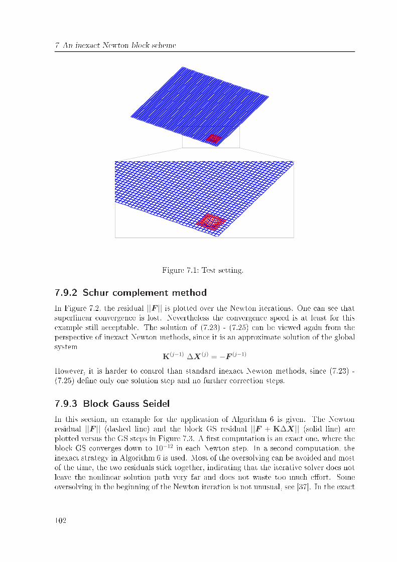
7 An inexa t Newton blo k s heme

Figure 7.1: Test setting.7.9.2 S hur omplement methodIn Figure 7.2, the residual ||F || is plotted over the Newton iterations. One an see thatsuperlinear onvergen e is lost. Nevertheless the onvergen e speed is at least for thisexample still a eptable. The solution of (7.23) - (7.25) an be viewed again from theperspe tive of inexa t Newton methods, sin e it is an approximate solution of the globalsystemK(j−1) ∆X (j) = −F (j−1)However, it is harder to ontrol than standard inexa t Newton methods, sin e (7.23) -(7.25) dene only one solution step and no further orre tion steps.7.9.3 Blo k Gauss SeidelIn this se tion, an example for the appli ation of Algorithm 6 is given. The Newtonresidual ||F || (dashed line) and the blo k GS residual ||F + K∆X|| (solid line) areplotted versus the GS steps in Figure 7.3. A rst omputation is an exa t one, where theblo k GS onverges down to 10−12 in ea h Newton step. In a se ond omputation, theinexa t strategy in Algorithm 6 is used. Most of the oversolving an be avoided and mostof the time, the two residuals sti k together, indi ating that the iterative solver does notleave the nonlinear solution path very far and does not waste too mu h eort. Someoversolving in the beginning of the Newton iteration is not unusual, see [37. In the exa t102

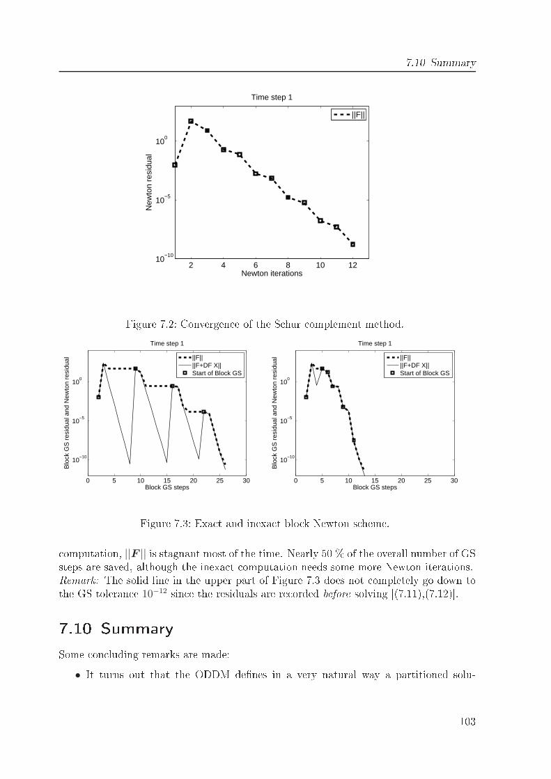
7.10 Summary

2 4 6 8 10 1210

−10

10−5

100

Newton iterations

New

ton

resi

dual

Time step 1

||F||

Figure 7.2: Convergen e of the S hur omplement method.

0 5 10 15 20 25 30

10−10

10−5

100

Blo

ck G

S r

esid

ual a

nd N

ewto

n re

sidu

al

Block GS steps

Time step 1

||F||||F+DF X||Start of Block GS

0 5 10 15 20 25 30

10−10

10−5

100

Blo

ck G

S r

esid

ual a

nd N

ewto

n re

sidu

al

Block GS steps

Time step 1

||F||||F+DF X||Start of Block GS

Figure 7.3: Exa t and inexa t blo k Newton s heme. omputation, ||F || is stagnant most of the time. Nearly 50 % of the overall number of GSsteps are saved, although the inexa t omputation needs some more Newton iterations.Remark: The solid line in the upper part of Figure 7.3 does not ompletely go down tothe GS toleran e 10−12 sin e the residuals are re orded before solving [(7.11),(7.12).7.10 SummarySome on luding remarks are made:• It turns out that the ODDM denes in a very natural way a partitioned solu-103

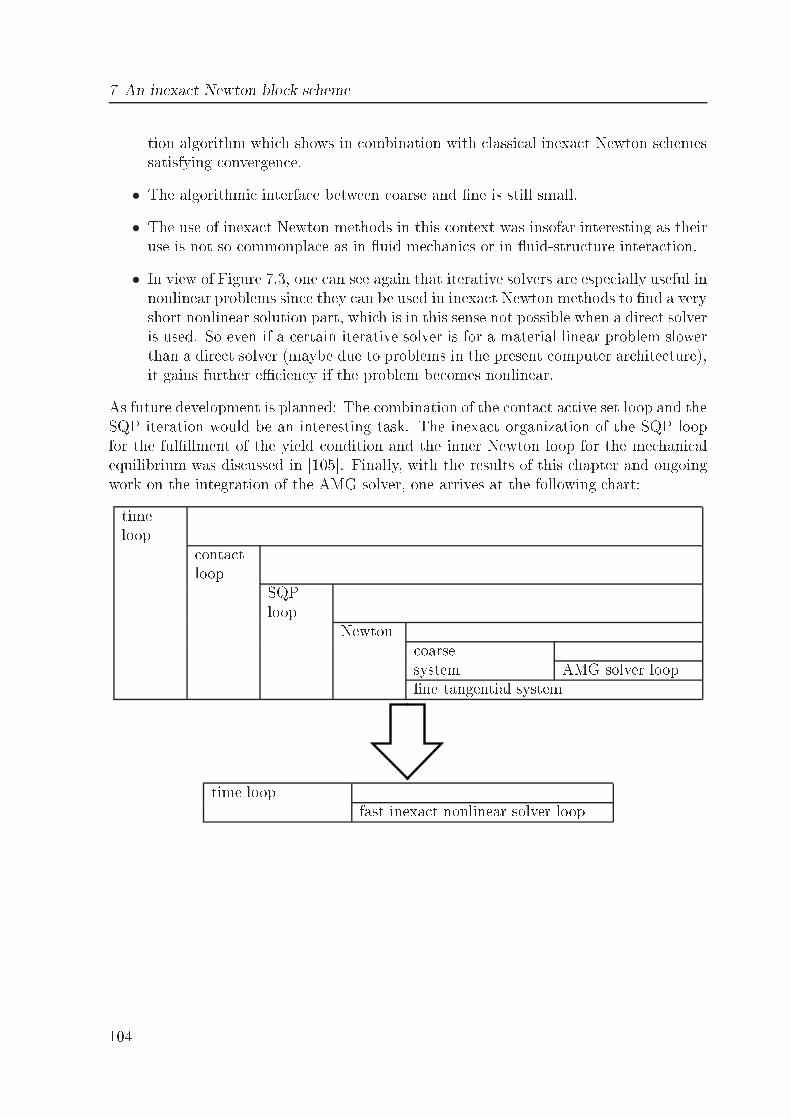
7 An inexa t Newton blo k s hemetion algorithm whi h shows in ombination with lassi al inexa t Newton s hemessatisfying onvergen e.• The algorithmi interfa e between oarse and ne is still small.• The use of inexa t Newton methods in this ontext was insofar interesting as theiruse is not so ommonpla e as in uid me hani s or in uid-stru ture intera tion.• In view of Figure 7.3, one an see again that iterative solvers are espe ially useful innonlinear problems sin e they an be used in inexa t Newton methods to nd a veryshort nonlinear solution part, whi h is in this sense not possible when a dire t solveris used. So even if a ertain iterative solver is for a material linear problem slowerthan a dire t solver (maybe due to problems in the present omputer ar hite ture),it gains further e ien y if the problem be omes nonlinear.As future development is planned: The ombination of the onta t a tive set loop and theSQP iteration would be an interesting task. The inexa t organization of the SQP loopfor the fulllment of the yield ondition and the inner Newton loop for the me hani alequilibrium was dis ussed in [105. Finally, with the results of this hapter and ongoingwork on the integration of the AMG solver, one arrives at the following hart:timeloop onta tloop SQPloop Newton oarsesystem AMG solver loopne tangential system

time loop fast inexa t nonlinear solver loop

104

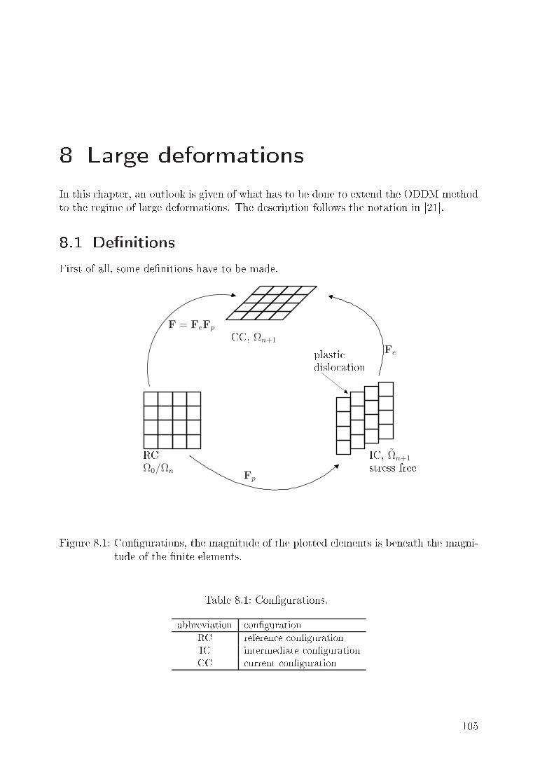
8 Large deformationsIn this hapter, an outlook is given of what has to be done to extend the ODDM methodto the regime of large deformations. The des ription follows the notation in [21.8.1 DenitionsFirst of all, some denitions have to be made.CC, Ωn+1

F = FeFp

Feplasti dislo ationIC, Ωn+1stress free

Fp

RCΩ0/Ωn

Figure 8.1: Congurations, the magnitude of the plotted elements is beneath the magni-tude of the nite elements.Table 8.1: Congurations.abbreviation ongurationRC referen e ongurationIC intermediate ongurationCC urrent onguration105

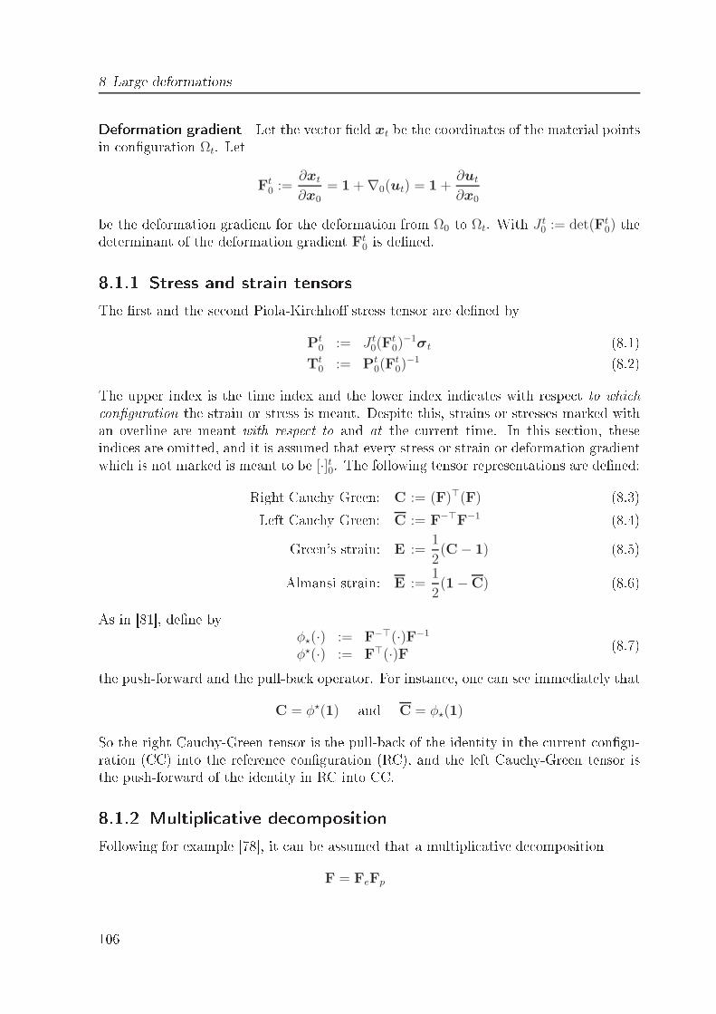
8 Large deformationsDeformation gradient Let the ve tor eld xt be the oordinates of the material pointsin onguration Ωt. LetFt

0 :=∂xt

∂x0

= 1 +∇0(ut) = 1 +∂ut

∂x0be the deformation gradient for the deformation from Ω0 to Ωt. With J t0 := det(Ft

0) thedeterminant of the deformation gradient Ft0 is dened.8.1.1 Stress and strain tensorsThe rst and the se ond Piola-Kir hho stress tensor are dened by

Pt0 := J t

0(Ft0)

−1σt (8.1)Tt

0 := Pt0(F

t0)

−1 (8.2)The upper index is the time index and the lower index indi ates with respe t to whi h onguration the strain or stress is meant. Despite this, strains or stresses marked withan overline are meant with respe t to and at the urrent time. In this se tion, theseindi es are omitted, and it is assumed that every stress or strain or deformation gradientwhi h is not marked is meant to be [·]t0. The following tensor representations are dened:Right Cau hy Green: C := (F)⊤(F) (8.3)Left Cau hy Green: C := F−⊤F−1 (8.4)Green's strain: E :=1

2(C− 1) (8.5)Almansi strain: E :=

1

2(1−C) (8.6)As in [81, dene by

φ⋆(·) := F−⊤(·)F−1

φ⋆(·) := F⊤(·)F (8.7)the push-forward and the pull-ba k operator. For instan e, one an see immediately thatC = φ⋆(1) and C = φ⋆(1)So the right Cau hy-Green tensor is the pull-ba k of the identity in the urrent ongu-ration (CC) into the referen e onguration (RC), and the left Cau hy-Green tensor isthe push-forward of the identity in RC into CC.8.1.2 Multipli ative de ompositionFollowing for example [78, it an be assumed that a multipli ative de omposition

F = FeFp106

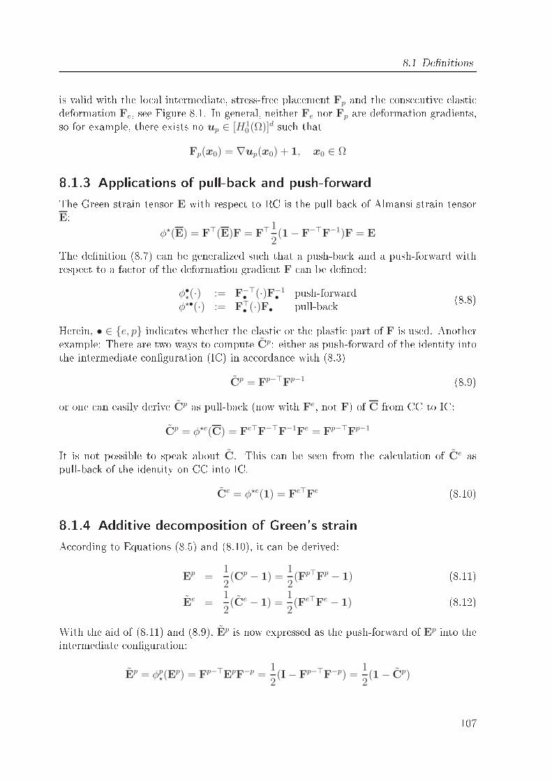
8.1 Denitionsis valid with the lo al intermediate, stress-free pla ement Fp and the onse utive elasti deformation Fe, see Figure 8.1. In general, neither Fe nor Fp are deformation gradients,so for example, there exists no up ∈ [H10 (Ω)]d su h that

Fp(x0) = ∇up(x0) + 1, x0 ∈ Ω8.1.3 Appli ations of pull-ba k and push-forwardThe Green strain tensor E with respe t to RC is the pull ba k of Almansi strain tensorE:

φ⋆(E) = F⊤(E)F = F⊤ 1

2(1− F−⊤F−1)F = EThe denition (8.7) an be generalized su h that a push-ba k and a push-forward withrespe t to a fa tor of the deformation gradient F an be dened:

φ•⋆(·) := F−⊤

• (·)F−1• push-forward

φ⋆•(·) := F⊤• (·)F• pull-ba k (8.8)Herein, • ∈ e, p indi ates whether the elasti or the plasti part of F is used. Anotherexample: There are two ways to ompute Cp: either as push-forward of the identity intothe intermediate onguration (IC) in a ordan e with (8.3)

Cp = Fp−⊤Fp−1 (8.9)or one an easily derive Cp as pull-ba k (now with Fe, not F) of C from CC to IC:Cp = φ⋆e(C) = Fe⊤F−⊤F−1Fe = Fp−⊤Fp−1It is not possible to speak about C. This an be seen from the al ulation of Ce aspull-ba k of the identity on CC into IC.

Ce = φ⋆e(1) = Fe⊤Fe (8.10)8.1.4 Additive de omposition of Green's strainA ording to Equations (8.5) and (8.10), it an be derived:Ep =

1

2(Cp − 1) =

1

2(Fp⊤Fp − 1) (8.11)

Ee =1

2(Ce − 1) =

1

2(Fe⊤Fe − 1) (8.12)With the aid of (8.11) and (8.9), Ep is now expressed as the push-forward of Ep into theintermediate onguration:

Ep = φp⋆(E

p) = Fp−⊤EpF−p =1

2(I− Fp−⊤F−p) =

1

2(1− Cp) 107

8 Large deformationsFurthermore, Ee an be understood with the aid of (8.11) and (8.12) as pull-ba k of Eefrom IC to RC.Ee = φ⋆p(Ee) = Fp⊤EeFp =

1

2(Fp⊤Fe⊤FeFp − Fp⊤Fp) =

1

2(C−Cp) (8.13)Remark: It is not possible to ompute Ee in terms of (8.5) as 1

2(F⊤

e Fe − I), sin e Ee isvalid with respe t to RC whereas Fe is living on RC.If one tries now to nd a meaningful additive de omposition of Green's strain tensor, onegets with (8.11) and (8.13) the following result:E =

1

2(C− 1) =

1

2(C−Cp) +

1

2(Cp − 1) = Ee + Ep (8.14)8.2 Equilibrium, Total LagrangeWith the results gathered in the last se tions, the Total Lagrange (TL) equilibrium anbe stated. At rst, some notations have to be laried. Let Ωn = Ωt be the last known onguration and let Ωn+1 = Ωt+∆t be the unknown onguration. By E(u;v), thedire tional derivative of E at u in dire tion of v is denoted:

E(u;v) := limk→0

1

k(E(u+ kv)−E(u))

= limk→0

1

2k(∇(kv) +∇(kv)⊤ +∇(kv)∇(kv)⊤ +∇(u)∇(kv)⊤ +∇(kv)∇(u)⊤)

= sym(∇(v)⊤ +∇(u)∇(v)⊤) (8.15)withsym(A) :=

1

2(A + A⊤)The main problem in the regime of large deformations is that the domain, where thesolution of the PDE has to be found, is solution dependent itself. This means that theweak form is stated with respe t to the unknown onguration Ωt+∆t. At the moment,only the internal for es are onsidered. Using

dΩt = J t0dΩ0 (8.16)

A : B = tr(AB) (8.17)∇t(·) = (Ft

0)−⊤∇0(·) (8.18)108

8.2 Equilibrium, Total Lagrangeand (8.1) as well as (8.2), it an be derived:f int(un+1,v) (8.19)

=

∫

Ωn+1

σn+1 : ∇n+1(v)⊤dΩn+1

=

∫

Ω0

Jn+10 σn+1 : ∇n+1(v)⊤dΩ0

=

∫

Ω0

(Fn+10 Pn+1

0 ) : ∇0(v)⊤(Fn+10 )−1dΩ0 (8.20)

=

∫

Ω0

Pn+10 : ∇0(v)⊤dΩ0

=

∫

Ω0

Tn+10 : (Fn+1

0 )⊤∇0(v)⊤dΩ0

=

∫

Ω0

Tn+10 : (1 +∇0(un+1))∇0(v)⊤dΩ0

=

∫

Ω0

Tn+10 : E(un+1;v) dΩ0 (8.21)The last equality holds be ause the se ond Piola Kir hho (PK) stress is a symmetri matrix. The gradient ∇n+1 omes from the strong form of the me hani al problem,where a divergen e operator is a ting with respe t to the urrent onguration. It isimportant to note, that if one writes ∇n+1(v) it is indeed meant ∇n+1(v ϕ−1) sin ethe test fun tion v is dened on the referen e domain Ω0. With this notation, Equation(8.20) be omes apparent (ϕ−1(xn+1) = x0):

∇n+1(v(ϕ−1(xn+1))) = ∇0(v)dϕ−1

dxn+1

= ∇0(v)(Fn+10 )−1In the following, this notation is omitted most of the time. In view of (8.21), it isinvestigated if the TL formulation is suitable for the ODDM. Therefore, the plasti statevariable Fp is assumed to be known in this se tion. If the St.Venant-Kir hho materiallaw T = CelEe is appli able, then the global equilibrium an be stated in this way:

∫

Ω0

E(un+1) : Cel : E(un+1;v) dΩ0 =

∫

Ω0

Ep : Cel : E(un+1;v) dΩ0 + ext. for es⇔

∫

Ω0

E(un+1) : Cel : E(un+1;v)−Ep : Cel : ∇0(un+1)∇0(v)⊤ dΩ0

=

∫

Ω0

Ep : Cel : ∇0(v)⊤dΩ0 + ext. for esTherefore, one nally arrives at a linear material (for known Ep), but still the followingdi ulties arise:1. A geometri nonlinear problem (expensive reassemblations of the oarse system inea h Newton step). 109

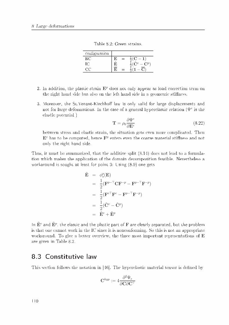
8 Large deformations Table 8.2: Green strains. ongurationRC E = 12(C− 1)IC E = 12(Ce −Cp)CC E = 12(1−C)2. In addition, the plasti strain Ep does not only appear as load orre tion term onthe right hand side but also on the left hand side in a geometri stiness.3. Moreover, the St.Venant-Kir hho law is only valid for large displa ements andnot for large deformations. In the ase of a general hyperelasti relation (Ψe is theelasti potential )

T = ρ0∂Ψe

∂Ee(8.22)between stress and elasti strain, the situation gets even more ompli ated. Then

Ee has to be omputed, hen e Fp enters even the oarse material stiness and notonly the right hand side.Thus, it must be summarized, that the additive split (8.14) does not lead to a formula-tion whi h makes the appli ation of the domain de omposition feasible. Nevertheless aworkaround is sought at least for point 3: Using (8.9) one getsE = φp

⋆(E)

=1

2(Fp−⊤CF−p − Fp−⊤F−p)

=1

2(Fe⊤Fe − Fp−⊤F−p)

=1

2(Ce − Cp)

= Ee + EpIn Ee and Ep, the elasti and the plasti part of F are learly separated, but the problemis that one annot work in the IC sin e it is non onforming. So this is not an appropriateworkaround. To give a better overview, the three most important representations of Eare given in Table 8.2.8.3 Constitutive lawThis se tion follows the notation in [46. The hyperelasti material tensor is dened byChyp := 4

∂2Ψe

∂C∂C⊤110

8.4 Consistent linearization of the onstitutive lawWithout deriving the onstitutive law, the four equations for the four unknown variablesT,α, Ep and λ are given:

T + λChyp :∂Φ

∂T− 1

2Chyp : C = 0 (8.23)

α+ λQ1(T,α) = 0 (8.24)Ep + λQ2(T,α) = 0 (8.25)

Φ(Ep,T,α) = 0 (8.26)withQ1 and Q2 denoting general onstitutive fun tions for the evolution of the ba kstressα and the plasti ar length Ep. The fun tion Q2 is assumed to be negative valued. Allother variables have been dened before. The KKT onditions have already entered(8.23)- (8.26). Of spe ial interest is (8.23), sin e it is an extra evolution equation forthe stress whi h does not appear in ommon plasti ity formulations. It is based on [51and enhan ed in [46. The advantage of this extra equation is that there is no longer aneed for an expli it ba k proje tion step whi h ne essitates in many ases an awkwardlinearization. With this method, only a full linearization of system (8.23) − (8.26) isne essary to ompute a stress whi h fullls the yield ondition.8.4 Consistent linearization of the onstitutive lawAfter time dis retization, two options are possible. Both options lead nally to the samelinear tangential stinesses:1. First linearize the ontinuous nonlinear bivariate form f int(u,v) in dire tion of aNewton in rement ∆u, and then dis retize the resulting bilinear and linear formsspatially.2. Perform the spatial dis retization before performing the Newton linearizations.In this hapter, the rst way is pursued, sin e it leads to a ompa t notation and itsupersedes the ne essity to write down the spatial dis retizations. Using (8.15) and thefa t that the dire tional derivative of ∇0(u) in dire tion of ∆u is ∇0(∆u) sin e thegradient is a linear fun tional, an auxiliary al ulation gives:

E(un+1; ∆u,v) = sym(∇0(∆u)∇0(v)⊤) (8.27)For omputing the Ja obian of f int(un+1;v) in Equation (8.19), one has to ompute thedire tional derivative in dire tion of the Newton in rement ∆u:f int(un+1,v; ∆u)

=

∫

Ω0

T(un+1; ∆u) : E(un+1;v) + T(un+1) : E(un+1;v,∆u) dΩ0

=

∫

Ω0

E(un+1; ∆u) : Cep : E(un+1;v) + T(un+1) : E(un+1;v,∆u) dΩ0

=

∫

Ω0

E(un+1; ∆u) : Cep : E(un+1;v) + T(un+1) :[

∇0(∆u)∇(v)⊤]

dΩ0 (8.28)111

8 Large deformationsAbove, (8.27) was used, as well as the denitionCep :=

dT(E)

dEwhi h is the subje t of the next se tion. The rst summand of (8.28) is the materialstiness and the se ond summand is the geometri stiness.8.5 A Gauss point se tion: Generalized proje tionmethodIt is explained in this last Gauss point se tion, how the elastoplasti tangent in (8.28) anbe omputed for a very general plasti ity model. It an be expe ted that the method, al-ready mentioned in Se tion 8.3 and whi h shall be named here as `generalized proje tion'method, will gain new interest in the FE simulation of in remental forming pro esses:The main disadvantage of the method is that a Newton iteration has to be performed forthe stress tensor and for the plasti data at ea h integration point. Sin e the zone, whereplasti state variables evolve, is relatively small in in remental pro esses, this disadvan-tage is outbalan ed by the advantage of the less omplex linearizations to be performed.Some notations: Let G be the nonlinear fun tional dened by the time dis retized versionof (8.23)-(8.26) and letz := (T,α, Ep, λ)⊤n+1 ∈ R

14be the ve tor 1 of unknowns. So the task is to nd some z⋆ su h thatG(z⋆(E⋆

n+1),E⋆n+1) = 0 (8.29)see [51 and the referen es therein. Herein, E⋆n+1 has the meaning of the total Greenstrain in the urrent Newton step. The impli it fun tion theorem states that there existopen sets U0 ⊃ E⋆

n+1 and V0 ⊃ z⋆(E⋆n+1) and an inje tive C1 mapping

z : U0 → V0su h thatG(z(En+1),En+1) = 0, En+1 ∈ U0Thus

dG

dEn+1|En+1=E⋆

n+1= 0

⇒ ∇zGdz

dEn+1|En+1=E⋆

n+1= − ∂G

∂En+1|En+1=E⋆

n+1(8.30)1It is not expli itly stated in this hapter when tensor values variables are meant to be in Voigt notation112

8.6 Updated LagrangeAlgorithm [T(j)n+1,C

ep,(j)n+1 ,α

(j)n+1] = GENERALIZED_PROJEC(E(j−1)

n+1 ,En,αn,Φ,Chyp)1. Compute trial values

Ttrn+1 := Tn + Chyp(E

(j−1)n+1 − En),C

ep,trn+1 := Chyp,αtr

n+1 := αn2. Che k yield onditionΦtr

n+1 := Φ(Ttrn+1,αn)IF Φtr

n+1 6 0 THEN: SET (•)(j)n+1 := (•)tr

n+1 AND EXITENDIF3. Solve problem (8.29) for [T(j)n+1,α

(j)n+1]4. Solve the 6 linear equation systems in (8.30) to get the onsistent elastoplasti tangent module as part of

dz(j)n+1

dE(j)n+1

= [Cep,(j)n+1 , . . .]

⊤8.6 Updated LagrangeFor a more detailed des ription of the updated Lagrange (UL) te hnique, see textbookslike for instan e [66 and the referen es therein. Let ∆un+1 := un+1−un be the in remen-tal displa ement from Ωn to Ωn+1. The main assumption of UL is that the ongurationsΩn and Ωn+1 are similar in the sense that in the load step tn → tn+1 the deformation isassumed to be small:

∫

Ωn+1

∆σn+1 : ∇n+1(v)⊤dΩn+1 ≈∫

Ωn

∆σn+1 : ∇n(v)⊤dΩn (8.31)It is important to note here, that ∆σn+1 on the left hand side is indeed related to the urrent onguration Ωn+1, a tually it is the push-forward of ∆Tn+1n , whereas ∆σn+1 onthe right hand side is related to Ωn and is meant in a small deformation manner. In thissense it should be made lear that ∆σn+1 = σn+1−σn is meaningless, sin e two stressesare subtra ted here whi h are measured with respe t to two dierent ongurations.Equation (8.31) shall be alled the assumption of small time steps. It means that thestress in rement ∆σn+1 whi h would be only valid with respe t to Ωn+1 in the ontextof large deformations between Ωn and Ωn+1, is assumed to be valid with respe t to Ωn.The assumption of small load steps an be justied, sin e otherwise the tool path is notresolved properly, see Figure 8.2. If the tool path is not resolved adequately then even themost sophisti ated impli it time integration of the onstitutive law and full linearizationof all bivariate forms will not redu e the error in the boundary onditions. On the other113

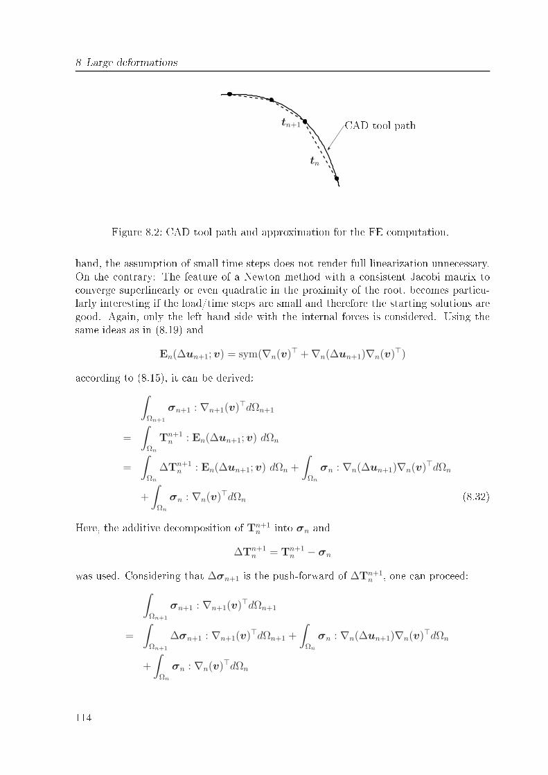
8 Large deformations

tn

tn+1 CAD tool pathFigure 8.2: CAD tool path and approximation for the FE omputation.hand, the assumption of small time steps does not render full linearization unne essary.On the ontrary: The feature of a Newton method with a onsistent Ja obi matrix to onverge superlinearly or even quadrati in the proximity of the root, be omes parti u-larly interesting if the load/time steps are small and therefore the starting solutions aregood. Again, only the left hand side with the internal for es is onsidered. Using thesame ideas as in (8.19) and

En(∆un+1;v) = sym(∇n(v)⊤ +∇n(∆un+1)∇n(v)⊤)a ording to (8.15), it an be derived:∫

Ωn+1

σn+1 : ∇n+1(v)⊤dΩn+1

=

∫

Ωn

Tn+1n : En(∆un+1;v) dΩn

=

∫

Ωn

∆Tn+1n : En(∆un+1;v) dΩn +

∫

Ωn

σn : ∇n(∆un+1)∇n(v)⊤dΩn

+

∫

Ωn

σn : ∇n(v)⊤dΩn (8.32)Here, the additive de omposition of Tn+1n into σn and

∆Tn+1n = Tn+1

n − σnwas used. Considering that ∆σn+1 is the push-forward of ∆Tn+1n , one an pro eed:

∫

Ωn+1

σn+1 : ∇n+1(v)⊤dΩn+1

=

∫

Ωn+1

∆σn+1 : ∇n+1(v)⊤dΩn+1 +

∫

Ωn

σn : ∇n(∆un+1)∇n(v)⊤dΩn

+

∫

Ωn

σn : ∇n(v)⊤dΩn114

8.6 Updated LagrangeWith the assumption (8.31), one arrives at:∫

Ωn+1

σn+1 : ∇n+1(v)⊤dΩn+1

≈∫

Ωn

∆σn+1 : ∇n(v)⊤ + σn : ∇n(∆un+1)∇n(v)⊤dΩn

+

∫

Ωn

σn : ∇n(v)⊤dΩn (8.33)=: f int

n (∆un+1;v) + f gn(∆un+1;v) + lgn(v) (8.34)The advantage of the formulation of the equilibrium in an updated Lagrange manner

f intn (∆un+1;v) + f g

n(∆un+1;v) = −lgn(v) + onta t for esis that on the left hand side, there is a problem, whi h is material nonlinear only in ∆u.With the aid of the ODDM, this an again be brought to the right hand side of the global oarse problem as load orre tion term. The ee tive stiness of the global problem hasto be updated in every load step due to the geometri stiness, whi h is still on the lefthand side, ontaining σn. But this is nevertheless far more advantageous than the TLformulation, sin e that would demand a global reassembly in ea h Newton step. One hasto onsider that the geometri nonlinearity is always a global one.8.6.1 Some iteration for ULOne an easily observe how large the error of the small-time-step assumption is, by he king the norm of the residual RUL whi h is dened as the standard FE assembly of∫

Ωn

∆σn+1 : ∇n(v)−∫

Ω(1)n+1

∆σn+1 : ∇n+1(v)withΩ

(1)n+1 := Ωn + ∆un+1Obviously, Ω

(1)n+1 is in general not equal to Ωn+1 sin e the in remental solution ∆un+1is only an approximation be ause the domain, where it was omputed, was Ωn and notthe orre t Ωn+1. A further development would be to perform an extra loop above thestru tural nonlinear solution pro ess and make the residualRUL,(l), whi h is the standardFE assembly of

∫

Ω(l−1)n+1

∆σ(l)n+1 : ∇n+1,l−1(v)−

∫

Ω(l)n+1

∆σ(l)n+1 : ∇n+1,l(v)vanish for l →∞. Here, Ω

(l)n+1 is dened byΩ

(0)n+1 := Ωn (8.35)

Ω(l)n+1 := Ωn + ∆u

(l)n+1, l = 1, . . . (8.36)115

8 Large deformationsPro eeding like this, the domain is updated in every step of the extra UL loop. Bathe [8states that it is possible to unroll the extra UL loop and the Newton loop su h the update(8.36) is performed in ea h Newton step. Of ourse in this ase, superlinear onvergen e annot be guaranteed anymore and for an a eptable onvergen e rate, the assumption(8.31) is again needed.8.7 Conta t Total LagrangeThe main issue of this se tion is the transmission of the onta t stresses from ne to oarse in the large deformation regime. Due to the large deformations and rigid bodymotions of the workpie e, the following question arises: In whi h onguration do themortar operator D and M need to be assembled? This question is answered exemplarilyfor M, sin e D depends only on the ne onta t interfa e whi h means that a hange ofthe onguration would not ause severe problems. However it is mu h more onvenientto set up M in the referen e onguration for the following reason: For many importantexamples for the ISF pro ess, the unma hined sheet an be assumed to be planar, su hthat ne grid and oarse grid t very well in the referen e onguration and translationalmovement of the ne grid with the tool auses no problem. This ni e property is lost,as soon as the oarse grid deforms due to the UL formulation. Then the biorthogonalityrelation hanges due to the fa t that a proje tion has to be performed to ompute theentries of M like it has to be done in the two-body onta t with urved interfa es. Inthe next se tion, it will be shown how the important integrals for M an be pulled ba kinto the referen e onguration.8.7.1 Transformation of the onta t stressesLet λn+1 be urrent onta t stress with respe t to time tn+1 and ϕ is the mappingΩ0 → Ωn+1. Then pro eed in this way:

∫

Γconn+1

λn+1(ϕ−1(xn+1)) · v(ϕ−1(xn+1)) dΓ

conn+1

=

∫

Γconn+1

[σn+1νn+1] (ϕ−1(xn+1)) · v(ϕ−1(xn+1)) dΓ

conn+1

=

∫

Γcon0

[

σn+1Jn+10 (Fn+1

0 )−1ν0

]

(x0) · v(x0) dΓcon0

=

∫

Γcon0

[

Pn+10 ν0

]

(x0) · v(x0) dΓcon0

=

∫

Γcon0

λn+10 (x0) · v(x0) dΓ

con0 (8.37)Again, Nanson's formula was used here in the form

νn+1dΓconn+1 = Jn+1

0 (Fn+10 )−1ν0 dΓ

con0116

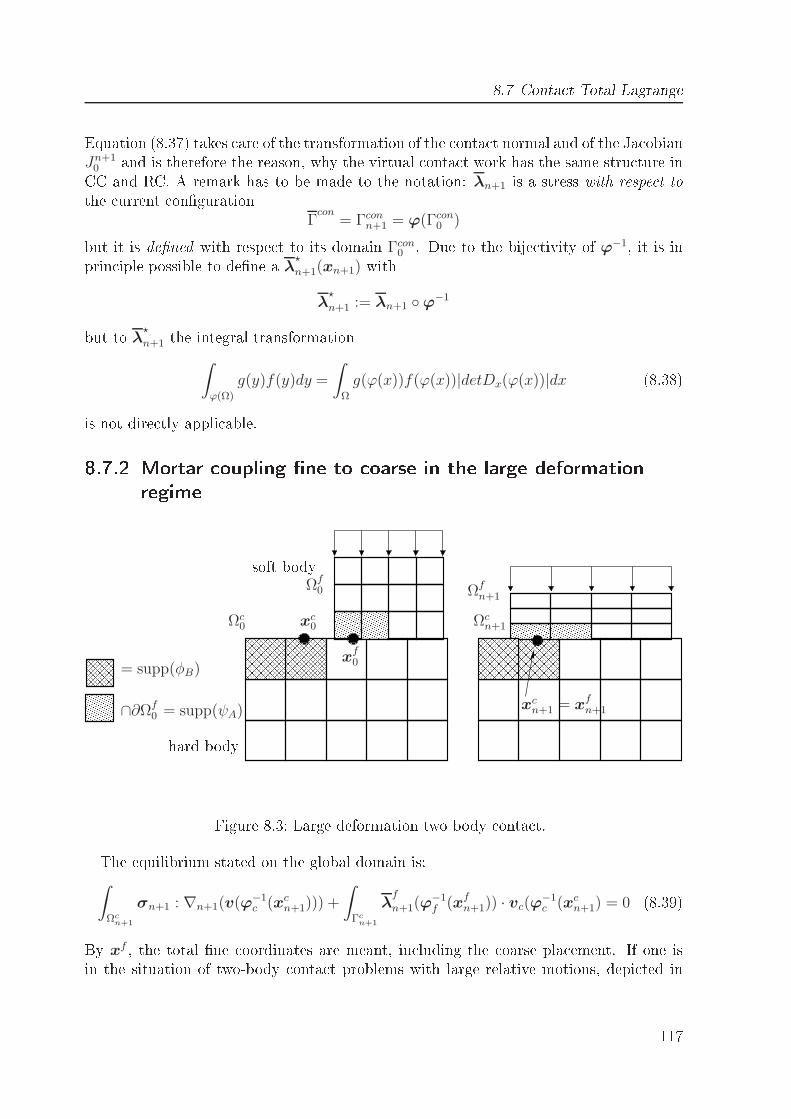
8.7 Conta t Total LagrangeEquation (8.37) takes are of the transformation of the onta t normal and of the Ja obianJn+1

0 and is therefore the reason, why the virtual onta t work has the same stru ture inCC and RC. A remark has to be made to the notation: λn+1 is a stress with respe t tothe urrent ongurationΓ

con= Γcon

n+1 = ϕ(Γcon0 )but it is dened with respe t to its domain Γcon

0 . Due to the bije tivity of ϕ−1, it is inprin iple possible to dene a λ⋆

n+1(xn+1) withλ

⋆

n+1 := λn+1 ϕ−1but to λ⋆

n+1 the integral transformation∫

ϕ(Ω)

g(y)f(y)dy =

∫

Ω

g(ϕ(x))f(ϕ(x))|detDx(ϕ(x))|dx (8.38)is not dire tly appli able.8.7.2 Mortar oupling ne to oarse in the large deformationregime

= supp(φB)

∩∂Ωf0 = supp(ψA)

xc0

xcn+1 = x

fn+1

xf0

Ωc0 Ωc

n+1

Ωfn+1

Ωf0

hard bodysoft body

Figure 8.3: Large deformation two body onta t.The equilibrium stated on the global domain is:∫

Ωcn+1

σn+1 : ∇n+1(v(ϕ−1c (xc

n+1))) +

∫

Γcn+1

λf

n+1(ϕ−1f (xf

n+1)) · vc(ϕ−1c (xc

n+1) = 0 (8.39)By xf , the total ne oordinates are meant, in luding the oarse pla ement. If one isin the situation of two-body onta t problems with large relative motions, depi ted in117

8 Large deformationsFigure 8.3, then it is impossible to apply (8.38) to the se ond summand and to pull itba k into the referen e onguration, sin e ϕ−1f 6= ϕ−1

c . For example in publi ations like[115, the operator M has to be set up in Γcn+1

M[A,B] =

∫

Γcn+1

ψB(ϕ−1f (xf

n+1))φA(ϕ−1c (xc

n+1))whi h means that it is solution dependent with all the awkward impli ations on erning onsistent linearization. In the ontext of this work, large relative motions of the twogrids are impossible sin e the ne grid solution does not substantially inuen e the oarsegrid solution. Therefore, the se ond summand of Problem (8.39) an be pulled ba k withthe aid of (8.37) into Γc0, and an be dis retized there. The ve tor Λ is then keeping thedis retized onta t stresses of λn+1

0 , whi h does not play a role for the evaluation of F con,as λn+10 and λn+1 dier only in a positive (even though spatially not onstant) fa tor.With Λ being meant in this way, one has to take are that the mortar operator D whi hdis retizes the oupling

∫

Γfn+1

λf

n+1(ϕ−1f (xf

n+1)) · vf (ϕ−1f (xf

n+1)has to be pulled ba k into RC, too. Otherwise the two mortar ouplings do not ttogether. On the other hand, the weak nonpenetration ondition has to be set up on Ωn,be ause the in remental displa ements are dis retized there.8.8 Con lusionsIt an be on luded that in the regime of large deformations, the ODDM is in prin iplepossible with a ne balan ed ombination of Total Lagrange and Updated Lagrangemethods, but both the volumetri and the surfa e oupling of the ne and the oarsegrid are di ult.• In prin iple, the mortar oupling of the onta t stress between ne and oarse gridis possible if1. The workpie e is planar and the assemblation is done in the referen e ong-uration or:2. Alternatively, one works with ompli ated proje tions.• Due to the deformation of the oarse grid and the ne grid, also the onstru tionof the data mapping operators PGP be omes very di ult.• The ODDM together with a purely total Lagrange approa h is not e ient sin ethe nonlinearities are not separated from the oarse grid omputation as it an bea hieved in the small deformation regime.

118

9 Con lusionsThis thesis is devoted to the Finite Element simulation of in remental metal formingpro esses. Several methods have been proposed to a elerate the Finite Element simula-tion whi h is very important to make it an attra tive alternative to trying out formingstrategies `by hand'.A large part has been dedi ated to the improvement of ommonly used onta t formu-lations, another one to the development of a partitioned solution approa h with a neFinite Element grid in the small and mobile forming zone and a oarse mesh for theglobal workpie e. In detail:• The importan e of orre t linearization of the elastoplasti onstitutive law in the ontext of metal forming pro esses has been underlined.• Several possibilities to solve the onstrained optimization problem of plasti ity havebeen shown and ompared.• The use of the primal dual a tive set strategy with dual Lagrange multipliers hasbeen studied, and its advantage over standard penalty methods has been shown innumeri al examples.• The onta t algorithm allows to apply fast iterative solvers on nonlinear problemsin a very e ient way.• It an be ombined with energy onservative s hemes in the impli it omputationof dynami al problems and it has been applied to a velo ity driven, rigid plasti problem.• The above mentioned divide-and- onquer approa h has been introdu ed to redu ethe number of unknowns in the Finite Element omputation.• The nonlinearities of the simulation, namely the onta t and the elastoplasti prob-lem have been hidden from the global omputation.• Due to lear data stru tures and a small interfa e, it turns out, that the ne gridand the oarse grid omputation an be distributed to two dierent FE odes.• The domain de omposition method is a dynami one, in the sense that the ne gridis travelling with the forming zone. 119

9 Con lusions• It denes in a very natural way a partitioned solution s heme whi h shows in ombination with inexa t Newton s hemes good onvergen e and nds a very shortnonlinear solution path.Based on the results of this work, several future developments are desirable.• The energy onsistent treatment of plasti ity in the regime of large deformationsshould be taken into a ount.• It should be intended to in orporate fri tional onta t into the proposed onta talgorithms.• A numeri al example in the ontext of an elasti problem showed that the ne and oarse grid are in prin iple independent. This result has to be extended to theelastoplasti ase by improving the data transfer operators.• It would be strongly desirable that the work is extended to the regime of largedeformations.• The proposed two-grid method should be ompared to adaptive methods with hang-ing nodes in terms of e ien y and a ura y. Nevertheless, the ODDM shouldnot be regarded as a method whi h is ompeting against more lassi al adaptives hemes. On the ontrary: It should be investigated, if both methods an ompleteone another.Overall, a signi ant speed in rease has been a hieved, by using several iterative solutionstrategies and domain de omposition methods. The proposed methods turn out to bepromising and worth to be tested in the framework of a ommer ial FEM pa kage tovalidate them for industrial appli ations.First steps in this dire tion have already been taken, for this thesis has been also intendedto make the nowadays still large gap between existing advan ed numeri al s hemes andthe needs of today's FEM software development a little bit smaller.

120

Bibliography[1 M. Ainsworth and J.T. Oden. A posteriori error estimation in nite element anal-ysis. Chi hester: Wiley, 2000. 73[2 P. Alart and A. Curnier. A mixed formulation for fri tional onta t problems proneto Newton like solution methods. Comput. Methods Appl. Me h. Engrg., 92:353375, 1991. 26, 27, 35, 43[3 H. Aretz. Modellierung des anisotropen Materialverhaltens von Ble hen mit Hilfeder Finite-Elemente-Methode. PhD thesis, Fakultät für Bergbau, Hüttenwesen undGeowissens haften, RWTH Aa hen, 2003. 8, 14, 16, 17[4 J.H. Argyris and J.S. Doltsinis. A primer on superplasti ity in natural formulation.Comput. Methods Appl. Me h. Engrg., 46:83131, 1984. 65[5 F. Armero and E. Peto z. A new lass of onserving algorithms for dynami onta tproblems. Comput. Methods Appl. Me h. Engrg., 158:269300, 1998. 54[6 I. Babu²ka and T. Strouboulis. The nite element method and its reliability. Oxford:Clarendon Press, 2001. 73[7 F. Barlat and J. Lian. Plasti behaviour and stret hibility of sheet metals. Part I:A yield fun tion for orthotropi sheets under plane stress ondition. InternationalJournal of Plasti ity, 95:1529, 1989. 8[8 K.J. Bathe. Finite Elemente Methoden. Springer, 1986. 116[9 F. Ben Belga em and Y. Renard. Hybrid nite element methods for the Signoriniproblem. Mathemati s of Computation, 72(243):11171145, 2003. 43[10 T. Belyts hko, W.K. Liu, and B. Moran. Nonlinear Finite Elements for Continuaand Stru tures. John Wiley & Sons, 2000. 7, 36[11 F. Ben Belga em, P. Hild, and P. Laborde. Approximation of the unilateral onta tproblem by the mortar nite element method. C. R. A sd. S i. Paris, 324:123127,1997. 43[12 F. Ben Belga em, P. Hild, and P. Laborde. Extension of the mortar nite ele-ment method to a variational inequality modeling unilateral onta t. Mathemati alModels and Methods in Applied S ien es, 9:287303, 1999. 43 121

Bibliography[13 M. Benzi. Pre onditioning te hniques for large linear systems: a survey. J. Comput.Phys., 182:418477, 2002. 31[14 C. Bernardi, Y. Maday, and A.T. Patera. A new non onforming approa h todomain de omposition: the mortar element method. In H. Brezzi et al., editor, In:Nonlinear partial dierential equations and their appli ations, pages 1351. Paris,1994. 43[15 M. Bis ho and E. Ramm. On the physi al signi an e of higher order kinemati and stati variables in a three-dimensional shell formulation. Internat. J. SolidsStru tures, 37:69336960, 2000. 53[16 W.L. Briggs, V.E. Henson, and S. M Cormi k. A Multigrid Tutorial, 2nd Edition.SIAM, Philadelphia, 2000. 31, 38[17 S. Brunssen. Modeling and simulation of elastoplasti forming pro esses. Te hni alReport 014, Universität Stuttgart, SPP 1146, 2006. 1, 4[18 S. Brunssen, S. Hüeber, and B. Wohlmuth. Conta t Dynami s with LagrangeMultipliers. In P. Wriggers and U. Na kenhorst, editors, Computational Methodsin Conta t Me hani s, volume 3 of IUTAM Bookseries, pages 1732. Springer, 2007.1, 4[19 S. Brunssen, F. S hmid, M. S häfer, and B. Wohlmuth. A fast and robust methodfor onta t problems by ombining a primal-dual a tive set strategy and algebrai multigrid. Internat. J. Numer. Methods Engrg., 69:524543, 2007. 1, 3, 25, 27[20 S. Brunssen and B. Wohlmuth. An overlapping domain de omposition method forthe simulation of elastoplasti in remental forming pro esses. Te hni al report,Universität Stuttgart, SPP 1146, 2007. Internat. J. Numer. Methods Engrg., toappear. 1, 4[21 A. Bu her. Deformationsgesetze für groÿe elastis h-plastis he Verzerrungen unterBerü ksi htigung einer Substruktur. PhD thesis, TU Chemnitz, 2001. 105[22 N. Bü hter and E. Ramm. 3D-extension of nonlinear shell equations based on theenhan ed assumed strain on ept. In C. Hirs h, editor, Computational Methods inApplied S ien es, pages 5562. Elsevier, 1992. 44, 53[23 N. Bü hter, E. Ramm, and D. Roehl. Three-dimensional extension of nonlinear shellformulation based on the enhan ed assumed strain on ept. Internat. J. Numer.Methods Engrg., 37:25512568, 1994. 53[24 G.T. Cama ho and M. Ortiz. Adaptive Lagrangian modelling of ballisti pene-tration of metalli targets. Comput. Methods Appl. Me h. Engrg., 142:347, 1997.89122

Bibliography[25 E. Ceretti, C. Giardini, and A. Attanasio. Sheet in remental forming on CNCma hines. In Pro eedings of the SheMet 2003, pages 4956, April 2003. 2[26 P.W. Christensen. A nonsmooth Newton method for elastoplasti problems. Com-put. Methods Appl. Me h. Engrg., 191:11891219, 2002. 35[27 P.W. Christensen and J.S. Pang. Fri tional onta t algorithms based on semis-mooth Newton methods. Internat. J. Numer. Methods Engrg., 42:145173, 1998.35, 43[28 J. Chung and G.M. Hulbert. A time integration algorithm for stru tural dynami swith improved numeri al dissipation: The Generalized-α method. J. Appl. Me h.,60:371375, 1993. 44, 50[29 W.J. Chung, J.W. Cho, and T. Belyts hko. On the dynami ee ts of expli it FEMin sheet metal forming analysis. Computational Me hani s, 15(6):750776, 1998. 3[30 T. Ci hosz. Simulation von inkrementellen Ble humformprozessen. Master's thesis,Institute of Stru tural Me hani s, Stuttgart, 2006. 57[31 A.J. Cleary, R.D. Falgout, V.E. Henson, J.E. Jones, T.A. Manteuel, S.F. M -Cormi k, G.N. Miranda, and J.W. Ruge. Robustness and s alability of algebrai multigrid. SIAM J. S i. Comput., 21(5):18861908, 2000. 27, 31[32 R.S. Dembo, S.C. Eisenstat, and T. Steighaug. Inexa t Newton methods. SIAMJ. Numer. Anal., 19:400408, 1982. 99[33 R. Diez, U. Hindenlang, and A. Kurz. LARSTRAN user's manual LARSTRANdo umentation. Te hni al report, Lasso GmbH, Stuttgart, 1996. 7, 36[34 Z. Dostal, A. Friedlander, and S.A. Santos. Solution of oer ive and semi oer ive onta t problems by FETI domain de omposition. Contemporary Mathemati s,218, 1998. 26[35 A. Düster, E. Rank, G. Steinl, and W. Wunderli h. A ombination of an h- and ap-version of the nite element method for elasti -plasti problems. In Pro eedingsof the ECCM 1999, September 1999. 73[36 S. E kert, H. Baaser, D. Gross, and O. S herf. A BDF2 integration method withstep size ontrol for elasto-plasti ity. Comput. Me h., 34:377386, 2004. 9[37 S.C. Eisenstat and H.F. Walker. Choosing the for ing terms in an inexa t Newtonmethod. SIAM J. S i. Comput., 17(1):1632, 1996. 96, 99, 102[38 K.A. Fis her and P. Wriggers. Fri tionless 2D onta t formulations for nite de-formations based on the mortar method. Comput. Me h., 36:226244, 2005. 43,76 123

Bibliography[39 J. Fish. The s-version of the nite element method. Computers and Stru tures,43:539547, 1992. 73[40 J. Fish and S. Markolefas. Adaptive s-method for linear elastostati s. Comput.Methods Appl. Me h. Engrg., 104:363396, 1993. 73[41 B. Flemis h. Non-mat hing Triangulations of Curvilinear Interfa es Applied toEle tro-Me hani s and Elasto-A ousti s. PhD thesis, Universität Stuttgart, ShakerVerlag, Aa hen, 2007. 32[42 B. Flemis h, J.M. Melenk, and B. Wohlmuth. Mortar methods with urved inter-fa es. Appl. Numer. Math., 54(3-4):339361, 2005. 83[43 B. Flemis h and B. Wohlmuth. Stable Lagrange multipliers for quadrilateral meshesof urved interfa es in 3D. Comput. Methods Appl. Me h. Engrg., 196(8):15891602,2007. 46[44 M. Gee, W.A. Wall, and E. Ramm. Parallel multilevel solution of nonlinear shellstru tures. Comput. Methods Appl. Me h. Engrg., 194:25132533, 2005. 53[45 R. Glowinski, J. He, A. Lozinski, J. Rappaz, and J. Wagner. Finite element ap-proximations of multis ale ellipti problems using pat hes of elements. Numer.Math., 101:663687, 2005. 74, 92[46 U.J. Görke, A. Bu her, Kreiÿig, and D. Mi hael. Ein Beitrag zur Lösung vonAnfangs-Randwert-Problemen eins hlieÿli h der Materialmodellierung bei nitenelastis h-plastis hen Verzerrungen mit Hilfe der FEM. Te hni al report, Preprint00-09 SFB 393, TU Chemnitz, 2000. 110, 111[47 A.M. Habraken and S. Ces otto. An automati remeshing te hnique for niteelement simulation of forming pro esses. Internat. J. Numer. Methods Engrg.,30:15031525, 1990. 89[48 W. Ha kbus h. MultiGrid Methods and Appli ations. Springer, 1985. 31, 38[49 W. Han and B.D. Reddy. Plasti ity, Mathemati al Theory and Numeri al Analysis.Springer, 1999. 7[50 S. Hartmann, S. Brunssen, E. Ramm, and B. Wohlmuth. A primal-dual a tive setstrategy for unilateral non-linear dynami onta t problems of thin-walled stru -tures. Internat. J. Numer. Methods Engrg., 70:883912, 2007. 1, 4, 32[51 S. Hartmann, G. Lührs, and P. Haupt. An e ient stress algorithm with ap-pli ations in vis oplasti ity and plasti ity. Internat. J. Numer. Methods Engrg.,40:9911013, 1997. 111, 112[52 P. Hauret and P. Le Talle . Energy- ontrolling time integration methods for nonlin-ear elastodynami s and low-velo ity impa t. Comput. Methods Appl. Me h. Engrg.,195:48904916, 2006. 53, 56124

Bibliography[53 M. Hintermüller, K. Ito, and K. Kunis h. The primal-dual a tive set strategy asa semismooth Newton method. SIAM Journal on Optimization, 13(3):865888,2003. 26, 27, 35, 43[54 G. Hirt, M. Bamba h, and S. Junk. Modelling of the in remental CNC sheet metalforming pro ess. In Pro eedings of the SheMet 2003, pages 495502, April 2003. 2[55 http://www.e oroll.de. 2[56 S. Hüeber, G. Stadler, and B. Wohlmuth. A primal-dual a tive set algorithm forthree-dimensional onta t problems with Coulomb fri tion. SIAM J. S i. Comput.,30(2):572596, 2008. 25[57 S. Hüeber and B. Wohlmuth. A primaldual a tive set strategy for nonlinearmultibody onta t problems. Comput. Methods Appl. Me h. Engrg., 194:31473166, 2005. 27, 43, 76[58 A. Hund and E. Ramm. Lo ality onstraints within multis ale model for non-linearmaterial behaviour. Internat. J. Numer. Methods Engrg., 70:16131632, 2007. 73[59 Simo J. and T.A. Laursen. Augmented Lagrangian treatment of onta t problemsinvolving fri tion. Comput. Stru t., 42:97116, 1992. 53[60 S. Junk. Inkrementelle Ble humformung mit CNC Werkzeugmas hinen: Ver-fahrensgrenzen und Umformstrategien. PhD thesis, Universität des Saarlandes,2003. 2[61 N. Kiku hi and Y. Joon Song. Penalty/nite-element approximations of a lass ofunilateral problems in linear elasti ity. Quarterly of Applied Mathemati s, 39:122,1981. 27[62 D. Klatte and B. Kummer. Nonsmooth Equations in Optimization, volume 60 ofNon onvex Optimization and Its Appli ations. Springer, 2002. 10[63 F. Klo ke and S. Mader. Fundamentals of the deep rolling of ompressor blades forturbo air raft engines. In Pro eedings of the 9th international onferen e on shotpeening, pages 125130, Paris, 2005. 1[64 D.A. Knoll and D.E. Keyes. Ja obian-free Newton-Krylov methods: a survey ofapproa hes and appli ations. J. Comput. Phys., 193:357397, 2004. 74[65 D.P. Koistinen and N.M. Wang. Me hani s of sheet metal forming - materialbehavior and deformation analysis. Plenum Press, 1978. 15[66 M. Koji¢ and K.J. Bathe. Inelasti Analysis of Solids and Stru tures. Springer,2005. 113[67 R. Kornhuber. Monotone multigrid methods for ellipti variational inequalities, I.Numer. Math., 69(2):167184, 1994. 26 125

Bibliography[68 R. Kornhuber and R. Krause. Adaptive multigrid methods for Signorini's problemin linear elasti ity. CVS, 4:920, 2001. 31[69 L. Krabbenhoft, A.V. Lyamin, S.W. Sloan, and P. Wriggers. An interior pointalgorithm for elastoplasti ity. Internat. J. Numer. Methods Engrg., 69:592626,2007. 20[70 R. Krause. Monotone Multigrid Methods for Signorini's Problem with Fri tion.PhD thesis, Freie Universität Berlin, 2001. 26, 31[71 R. Krause and E. Rank. Multis ale omputations with a ombination of the h-and p-versions of the nite element method. Comput. Methods Appl. Me h. Engrg.,192:39593983, 2003. 73[72 E. Kröner. Benets and short omings of the ontinuous theory of dislo ations.Internat. J. Solids Stru tures, 38:11151134, 2001. 94[73 D. Kuhl and M.A. Criseld. Energy onserving and de aying algorithms in non-linear stru tural dynami s. Internat. J. Numer. Methods Engrg., 45:569599, 1999.50[74 D. Kuhl and E. Ramm. Generalized energy-momentum method for non-linearadaptive shell dynami s. Comput. Methods Appl. Me h. Engrg., 178:343366, 1999.44, 50[75 T.A. Laursen. Computational Conta t and Impa t Me hani s. Springer, 2002. 25,53[76 T.A. Laursen and V. Chawla. Design of energy onserving algorithms for fri tionlessdynami onta t problems. Internat. J. Numer. Methods Engrg., 40:863886, 1997.54[77 T.A. Laursen and G.R. Love. Improved impli it integrators for transient impa tproblems - geometri admissibility within the onserving framework. Internat. J.Numer. Methods Engrg., 53:245274, 2002. 44, 54, 56, 63[78 E.H. Lee. Elasti -plasti deformation at nite strains. J. Appl. Me h., 36:16, 1969.106[79 N.S. Lee and K.J. Bathe. Error indi ators and adaptive remeshing in large defor-mation nite element analyis. Fin. El. in Analysis and Design, 116:99139, 1994.89[80 S.H Lee, J.H. Song, Y.C. Yoon, G. Zi, and T. Belyts hko. Combined extendedand superimposed nite element method for ra ks. Internat. J. Numer. MethodsEngrg., 59:11191136, 2004. 73126

Bibliography[81 J.E. Marsden and T.J.R. Hughes. Mathemati al Foundations of Elasti ity. Prenti e-Hall International In ., 1983. 106[82 T.W. M Devitt and T.A. Laursen. A mortar nite element formulation for fri tional onta t problems. Internat. J. Numer. Methods Engrg., 48:15251547, 2000. 43, 76[83 K. M Loughlin, A. Cognot, and E. Quigley. Dieless manufa turing of sheet metal omponents with non rigid support. In Pro eedings of the SheMet 2003, pages123130, April 2003. 2[84 T. Meinders, A.H. van den Boogaard, and J. Huétink. Improvement of impli itnite element ode performan e in deep drawing simulations by dynami s ontri-butions. J. of Materials Pro essing Te hnology, 134:413420, 2003. 4[85 A. Meyer. Proje ted PCGM for handling hanging nodes in adaptive nite elementpro edures. Te hni al report, Preprint 99-25 SFB 393, TU Chemnitz, 1999. 89[86 R. Mohr, A. Menzel, and P. Steinmann. Conservation properties of galerkin-basedtime-stepping s hemes for nite elasto-plasto-dynami s. In R. Owen, E. Onate,and B. Suarez, editors, Computational Plasti ity IX, pages 948951. Int. Center forNumeri al Methods in Engrg., CIMNE, September 2007. 4[87 M. Oldenburg and L. Nilsson. The position ode algorithm for onta t sear hing.Internat. J. Numer. Methods Engrg., 37:359386, 1994. 77[88 V. Padmanabhan and T.A. Laursen. Surfa e smoothing pro edure for large defor-mation onta t analysis. Finite Elem. Anal. Des., 37:173198, 2001. 43[89 P. Papadopoulos and R. Taylor. A mixed formulation for the nite element solutionof onta t problems. Comput. Methods Appl. Me h. Engrg., 94:373389, 1992. 43,82[90 J. Pebrel, P. Gosselet, and C. Rey. Multis ale analysis of stru tures using overlap-ping nonlinear pat hes. In E. Onate, M. Papadrakakis, and B. S hreer, editors,Computational Methods for Coupled Problems in S ien e and Engineering II, pages453456. Int. Center for Numeri al Methods in Engrg., CIMNE, May 2007. 74[91 M.A. Puso and T.A. Laursen. A 3D onta t smoothing method using Gregorypat hes. Internat. J. Numer. Methods Engrg., 54:11611194, 2002. 43[92 M.A. Puso and T.A. Laursen. A mortar segmenttosegment onta t method forlarge deformation solid me hani s. Comput. Methods Appl. Me h. Engrg., 193:601629, 2004. 25, 43, 76[93 M.A. Puso and T.A. Laursen. A mortar segment-to-segment fri tional onta tmethod for large deformations. Comput. Methods Appl. Me h. Engrg., 193:48914913, 2004. 43 127

Bibliography[94 E. Rank, A. Düster, D. Ledentsov, I. Heinle, W. Volk, and M. Wagner. A uniedapproa h to multis ale simulation and dimensional adaptivity: basi prin iples andindustrial appli ations. In E. Onate, M. Papadrakakis, and B. S hreer, editors,Computational Methods for Coupled Problems in S ien e and Engineering II, pages649652. Int. Center for Numeri al Methods in Engrg., CIMNE, May 2007. 73[95 J.W. Ruge and K. Stüben. Multigrid Methods, Frontiers in Applied Mathemati s,volume 3, hapter Algebrai Multigrid, pages 73130. SIAM, Philadelphia, 1987.31[96 Y. Saad. Iterative Methods for Sparse Linear Systems, 2nd Edition. SIAM, Philadel-phia, 2003. 94, 97[97 J.C. Simo and T.J.R. Hughes. Computational Inelasti ity. Springer, 1998. 7, 9, 10,13, 14, 23[98 J.C. Simo and M. Ortiz. A unied approa h to nite deformation elastoplasti analysis based on the use of hyperelasti onstitutive equations. Comput. MethodsAppl. Me h. Engrg., 49:221245, 1985. 14[99 J.C. Simo and R.L. Taylor. Consistent tangent operators for rate independentelasto-plasti ity. Comput. Methods Appl. Me h. Engrg., 48:101118, 1985. 9[100 M. Stadler and G.A. Holzapfel. Subdivision s hemes for smooth onta t surfa es ofarbitrary mesh topology in 3D. Internat. J. Numer. Methods Engrg., 60:11611195,2004. 43[101 E. Stein and M. Rüter. Finite element methods for elasti ity with error- ontrolleddis retization and model adaptivity. In E. Stein, R. de Borst, and J.R. Hughes,editors, En y lopedia of Computational Me hani s, volume 2, hapter 2, pages 558. John Wiley & Sons, 2004. 73[102 K. Stüben. A review of algebrai multigrid. J. Comput. Appl. Math., 128:281309,2001. 27, 31[103 M. Tabbara, T. Bla ker, and T. Belyts hko. Finite element derivative re overy bymoving least square interpolants. Comput. Methods Appl. Me h. Engrg., 117:211223, 1994. 89[104 R. Verfürth. A review of a posteriori error estimation and adaptive mesh-renementte hniques. WileyTeubner Series Advan es in Numeri al Mathemati s. WileyTeubner, Chi hester, Stuttgart, 1996. 73[105 C. Wieners. Nonlinear solution methods for innitesimal perfe t plasiti ity. Z.Angew. Math. Me h., 87(8):643660, 2007. 17, 19, 73, 104[106 K. Willner. Kontinuums- und Kontaktme hanik. Springer, 2003. 25, 39128

Bibliography[107 B. Wohlmuth. A mortar nite element method using dual spa es for the Lagrangemultiplier. SIAM J. Numer. Anal., 38:9891012, 2000. 43[108 B. Wohlmuth. Dis retization te hniques and iterative solvers based on domainde omposition. Le ture Notes in Computational S ien e and Engineering, 17, 2001.Springer. 27, 32[109 P. Wriggers. Ni htlineare Finite-Element-Methoden. Springer, 2001. 7[110 P. Wriggers. Computational Conta t Me hani s. John Wiley & Sons, 2002. 25[111 P. Wriggers and K. Fis her. Re ent new developments in onta t me hani s. InPro eedings of the 4th European LS-DYNA Users Conferen e, Ulm, 2003. 25[112 P. Wriggers and G. Zavarise. En y lopedia of Computational Me hani s, volume 2, hapter Computational Conta t Me hani s. John Wiley & Sons, 2004. 25[113 S.P. Xiao and T. Belyts hko. A bridging domain method for oupling ontinuawith mole ular dynami s. Comput. Methods Appl. Me h. Engrg., 193:16451669,2004. 74[114 B. Yang and T.A. Laursen. A onta t sear hing algorithm in luding bounding vol-ume trees applied to nite sliding mortar formulations. Computational Me hani s,41:189205, 2008. 77[115 B. Yang, T.A. Laursen, and X.N. Meng. Two dimensional mortar onta t meth-ods for large deformation fri tional sliding. Internat. J. Numer. Methods Engrg.,62:11831225, 2005. 29, 43, 118[116 Z. Yue and D.H. Robbins. Adaptive superposition of nite element meshes inelastodynami problems. Internat. J. Numer. Methods Engrg., 63(11):16041635,2005. 73

129