CIVE 702 MIDTERM WINTER 2015

Cyle Teal CIVE 702 February 12, 2015

Table of Contents INTRODUCTION .......................................................................................................... 1

FLEXIBILITY MATRIX COMPUTATION .................................................................... 2

Beam length ............................................................................................................... 2

Geometric centroid .................................................................................................... 2

Principal Second Moments of Area ........................................................................... 2

Polar Second Moment of Area .................................................................................. 2

Shear Center ............................................................................................................... 3

Material Properties .................................................................................................... 3

Flexibility Matrix ........................................................................................................ 3

SECTION PROPERTY COMPARISON......................................................................... 3

Discussion .................................................................................................................. 4

STRESS COMPUTATION ............................................................................................. 4

Bending ....................................................................................................................... 4

Shear Stress ................................................................................................................ 5

Shear Area .................................................................................................................. 6

Torsion ........................................................................................................................ 7

DISPLACEMENT COMPUTATION ............................................................................. 7

Comparison .............................................................................................................. 10

CONCLUSION ............................................................................................................ 10

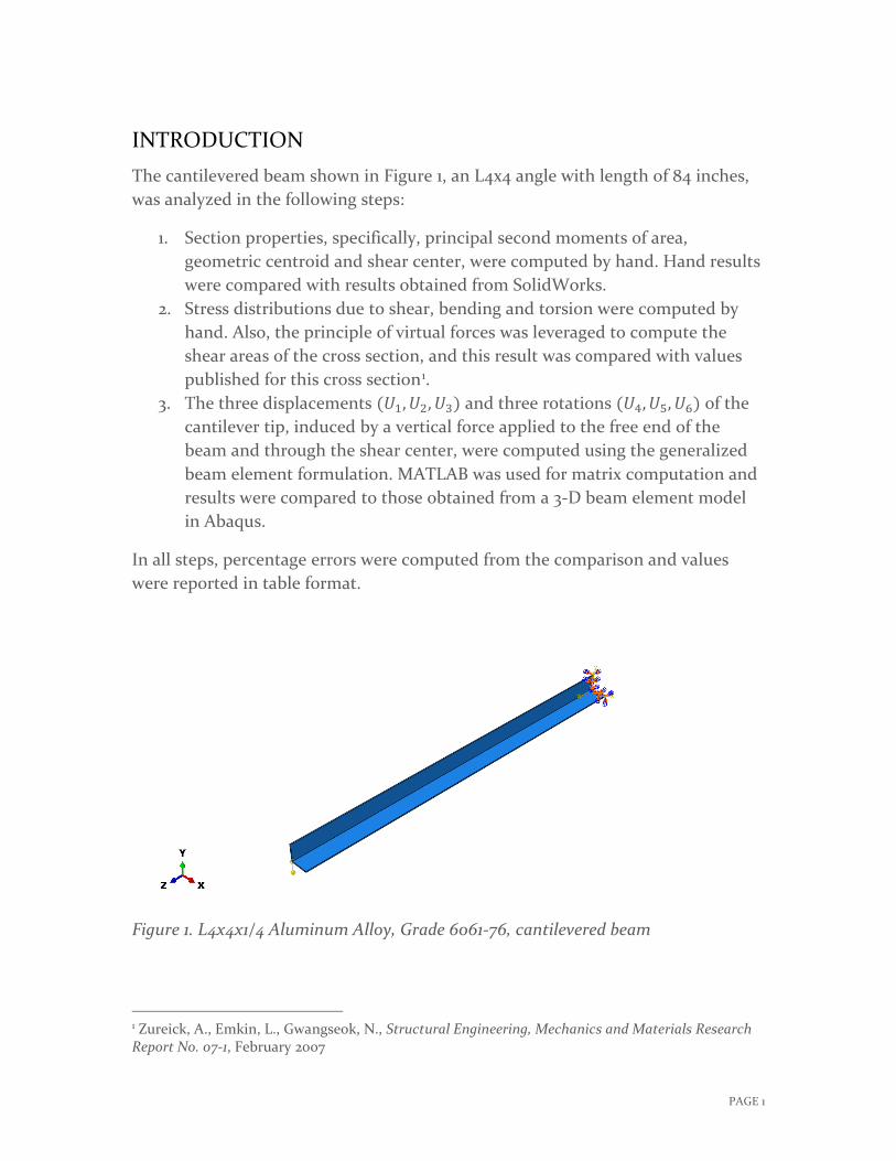
INTRODUCTION The cantilevered beam shown in Figure 1, an L4x4 angle with length of 84 inches, was analyzed in the following steps:

1. Section properties, specifically, principal second moments of area, geometric centroid and shear center, were computed by hand. Hand results were compared with results obtained from SolidWorks.

2. Stress distributions due to shear, bending and torsion were computed by hand. Also, the principle of virtual forces was leveraged to compute the shear areas of the cross section, and this result was compared with values published for this cross section1.

3. The three displacements (𝑈𝑈1,𝑈𝑈2,𝑈𝑈3) and three rotations (𝑈𝑈4,𝑈𝑈5,𝑈𝑈6) of the cantilever tip, induced by a vertical force applied to the free end of the beam and through the shear center, were computed using the generalized beam element formulation. MATLAB was used for matrix computation and results were compared to those obtained from a 3-D beam element model in Abaqus.

In all steps, percentage errors were computed from the comparison and values were reported in table format.

Figure 1. L4x4x1/4 Aluminum Alloy, Grade 6061-76, cantilevered beam

1 Zureick, A., Emkin, L., Gwangseok, N., Structural Engineering, Mechanics and Materials Research Report No. 07-1, February 2007

PAGE 1

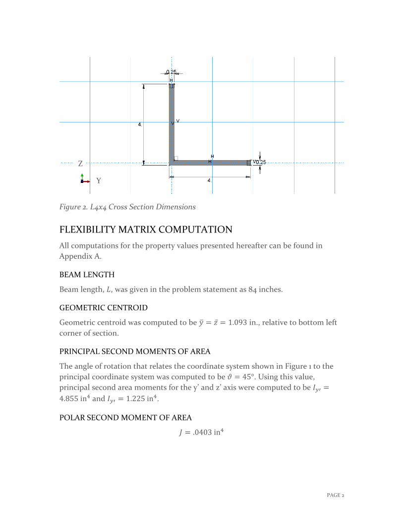
Figure 2. L4x4 Cross Section Dimensions

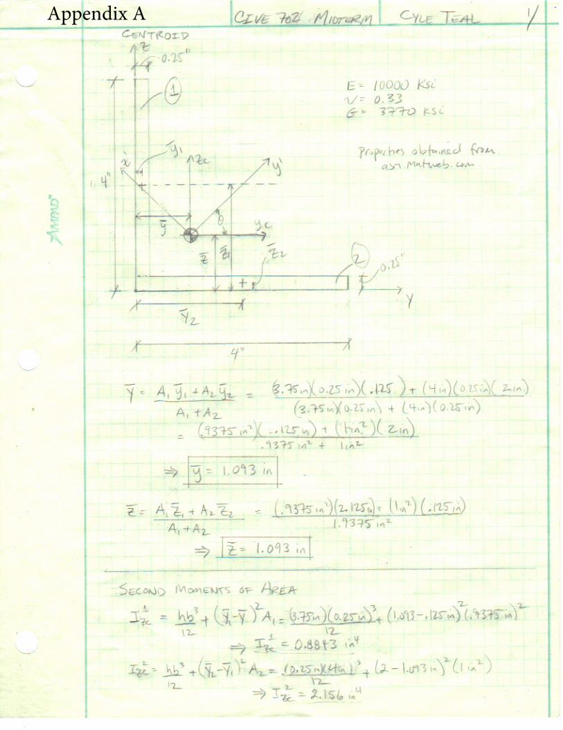
FLEXIBILITY MATRIX COMPUTATION All computations for the property values presented hereafter can be found in Appendix A.

BEAM LENGTH

Beam length, 𝐿𝐿, was given in the problem statement as 84 inches.

GEOMETRIC CENTROID

Geometric centroid was computed to be 𝑦𝑦� = 𝑧𝑧̅ = 1.093 in., relative to bottom left corner of section.

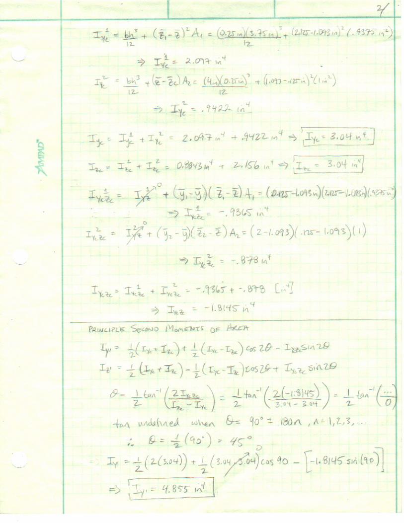
PRINCIPAL SECOND MOMENTS OF AREA

The angle of rotation that relates the coordinate system shown in Figure 1 to the principal coordinate system was computed to be 𝜗𝜗 = 45°. Using this value, principal second area moments for the y’ and z’ axis were computed to be 𝐼𝐼𝑦𝑦′ =4.855 in4 and 𝐼𝐼𝑦𝑦′ = 1.225 in4.

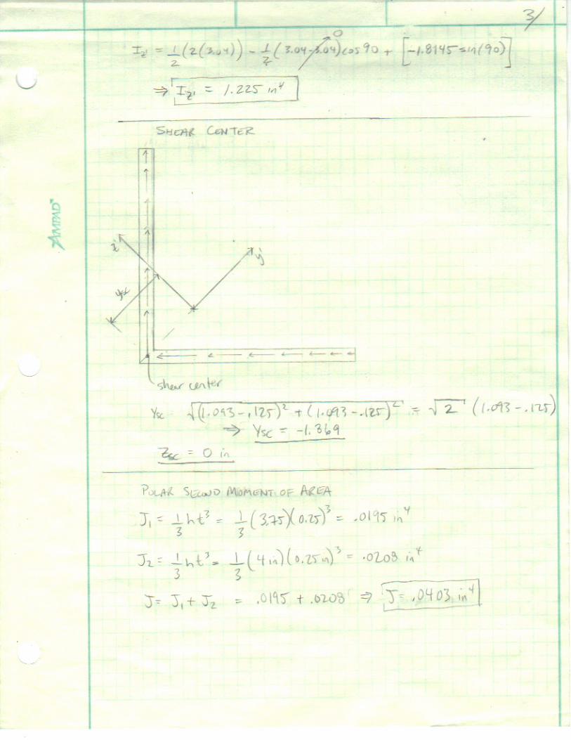
POLAR SECOND MOMENT OF AREA

𝐽𝐽 = .0403 in4

Y

Z

PAGE 2

SHEAR CENTER

The following values for location of the shear center are given in the principal coordinate system with origin located at geometric centroid

𝑦𝑦𝑠𝑠𝑠𝑠 = −1.369 in

𝑧𝑧𝑠𝑠𝑠𝑠 = 0 in

MATERIAL PROPERTIES

Modulus of Elasticity, Shear Modulus, and Poisson’s ratio for Grade 6061-T6 aluminum obtained from asm.matweb.com

𝐸𝐸 = 10E + 07 psi

𝐺𝐺 = 3.77E + 06 psi

𝜈𝜈 = 0.33

FLEXIBILITY MATRIX

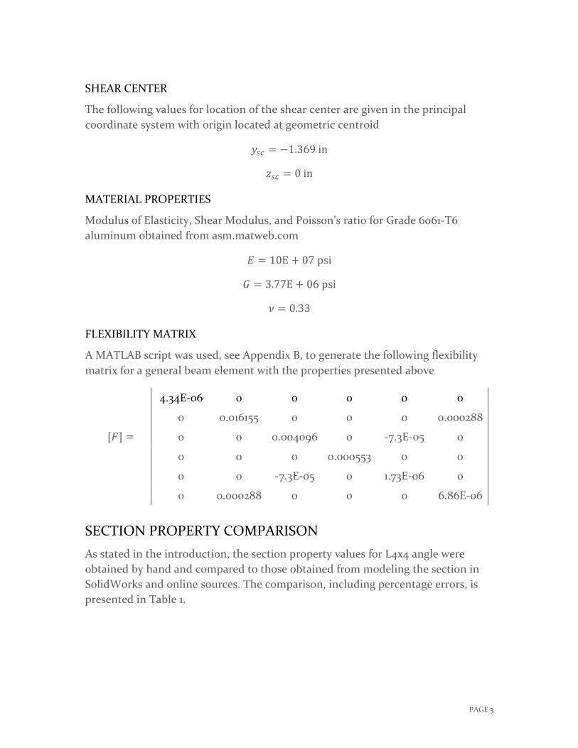
A MATLAB script was used, see Appendix B, to generate the following flexibility matrix for a general beam element with the properties presented above

4.34E-06 0 0 0 0 0

0 0.016155 0 0 0 0.000288

[𝐹𝐹] = 0 0 0.004096 0 -7.3E-05 0

0 0 0 0.000553 0 0

0 0 -7.3E-05 0 1.73E-06 0

0 0.000288 0 0 0 6.86E-06

SECTION PROPERTY COMPARISON As stated in the introduction, the section property values for L4x4 angle were obtained by hand and compared to those obtained from modeling the section in SolidWorks and online sources. The comparison, including percentage errors, is presented in Table 1.

PAGE 3

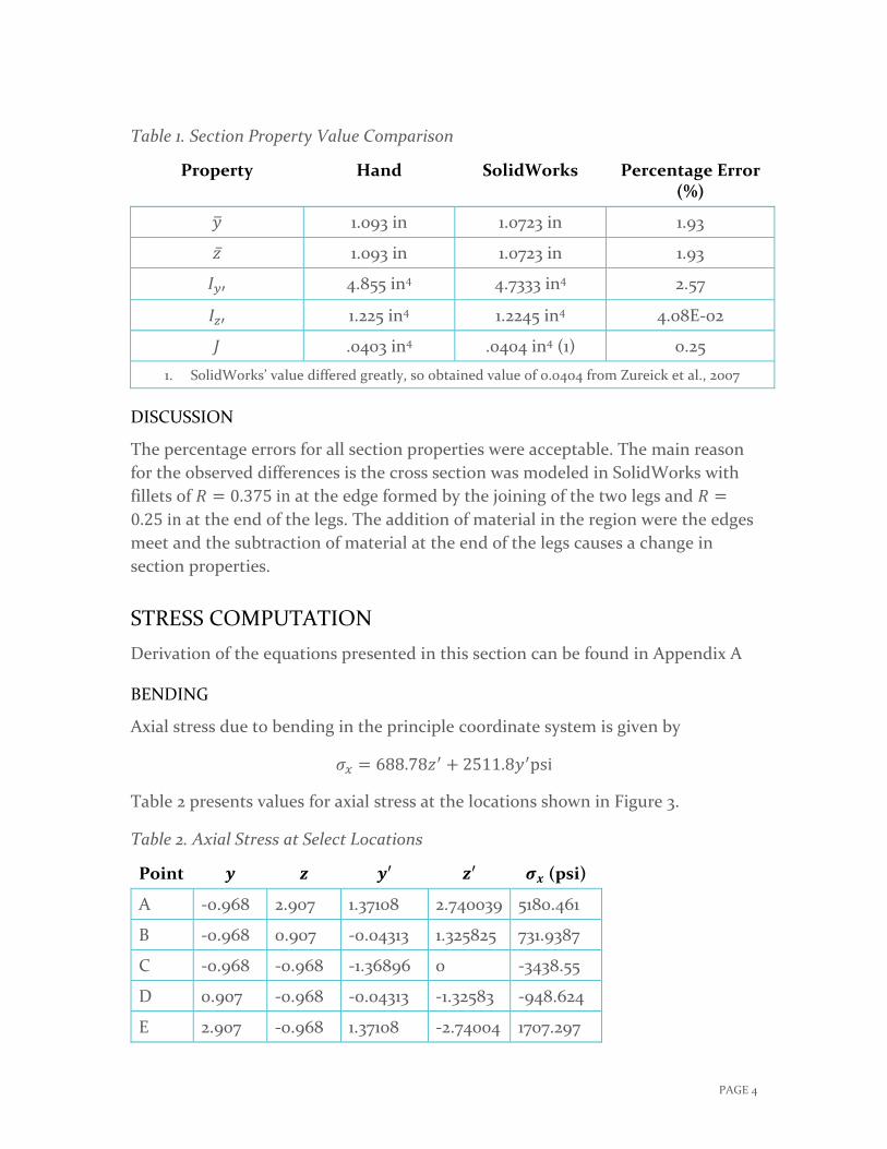
Table 1. Section Property Value Comparison

Property Hand SolidWorks Percentage Error (%)

𝑦𝑦� 1.093 in 1.0723 in 1.93

𝑧𝑧̅ 1.093 in 1.0723 in 1.93

𝐼𝐼𝑦𝑦′ 4.855 in4 4.7333 in4 2.57

𝐼𝐼𝑧𝑧′ 1.225 in4 1.2245 in4 4.08E-02

𝐽𝐽 .0403 in4 .0404 in4 (1) 0.25

1. SolidWorks’ value differed greatly, so obtained value of 0.0404 from Zureick et al., 2007

DISCUSSION

The percentage errors for all section properties were acceptable. The main reason for the observed differences is the cross section was modeled in SolidWorks with fillets of 𝑅𝑅 = 0.375 in at the edge formed by the joining of the two legs and 𝑅𝑅 =0.25 in at the end of the legs. The addition of material in the region were the edges meet and the subtraction of material at the end of the legs causes a change in section properties.

STRESS COMPUTATION Derivation of the equations presented in this section can be found in Appendix A

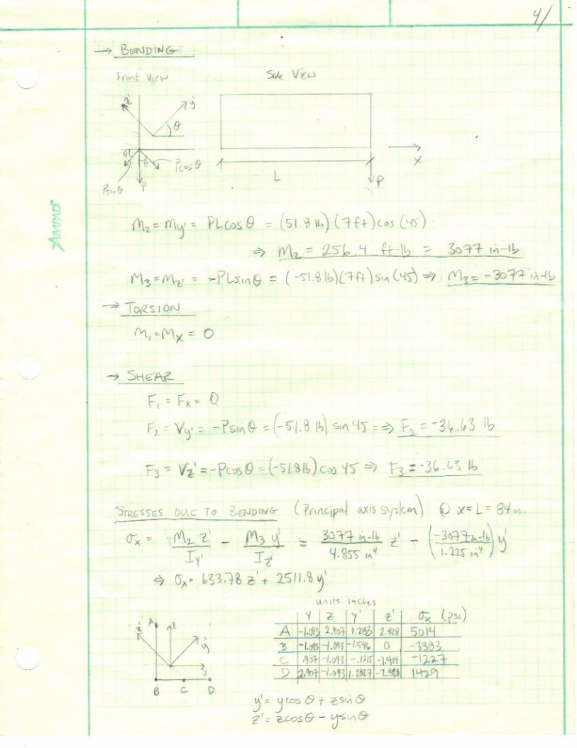
BENDING

Axial stress due to bending in the principle coordinate system is given by

𝜎𝜎𝑥𝑥 = 688.78𝑧𝑧′ + 2511.8𝑦𝑦′psi

Table 2 presents values for axial stress at the locations shown in Figure 3.

Table 2. Axial Stress at Select Locations

Point 𝒚𝒚 𝒛𝒛 𝒚𝒚′ 𝒛𝒛′ 𝝈𝝈𝒙𝒙 (psi)

A -0.968 2.907 1.37108 2.740039 5180.461

B -0.968 0.907 -0.04313 1.325825 731.9387

C -0.968 -0.968 -1.36896 0 -3438.55

D 0.907 -0.968 -0.04313 -1.32583 -948.624

E 2.907 -0.968 1.37108 -2.74004 1707.297

PAGE 4

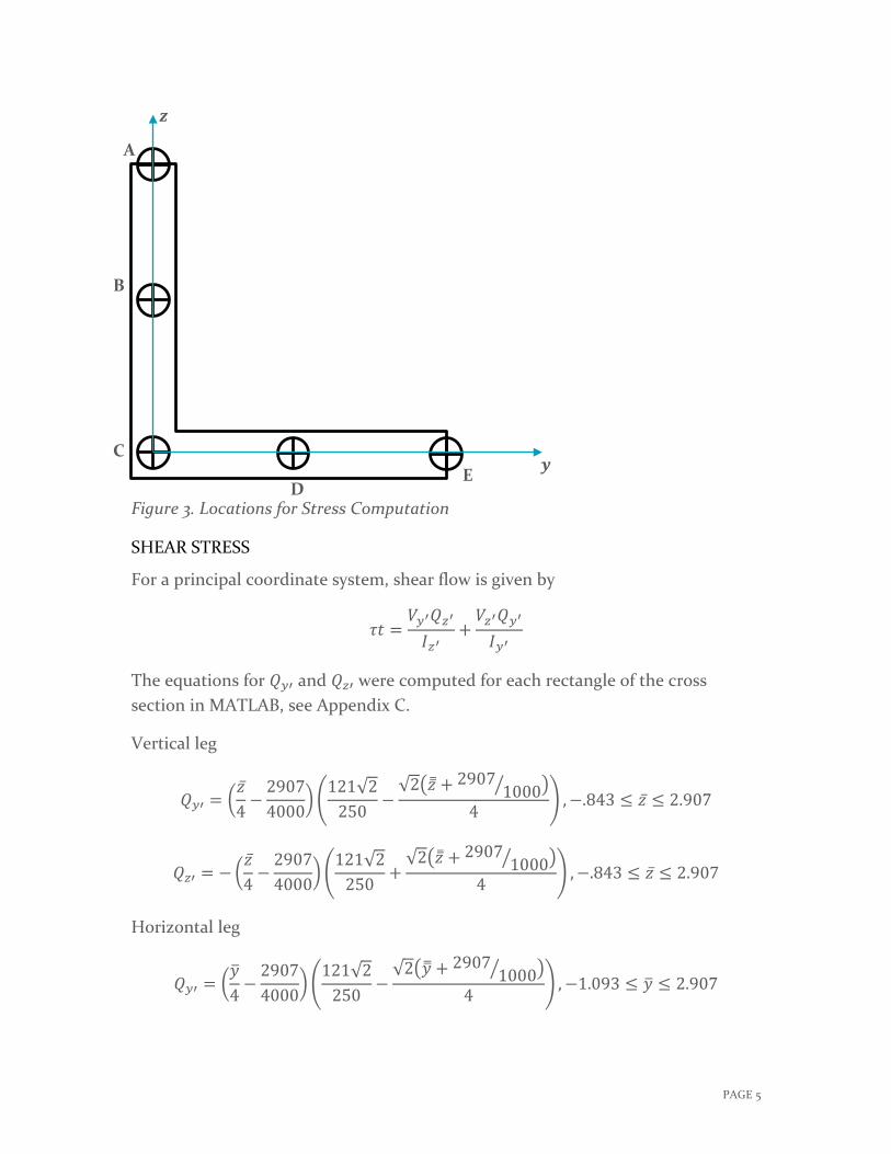
Figure 3. Locations for Stress Computation

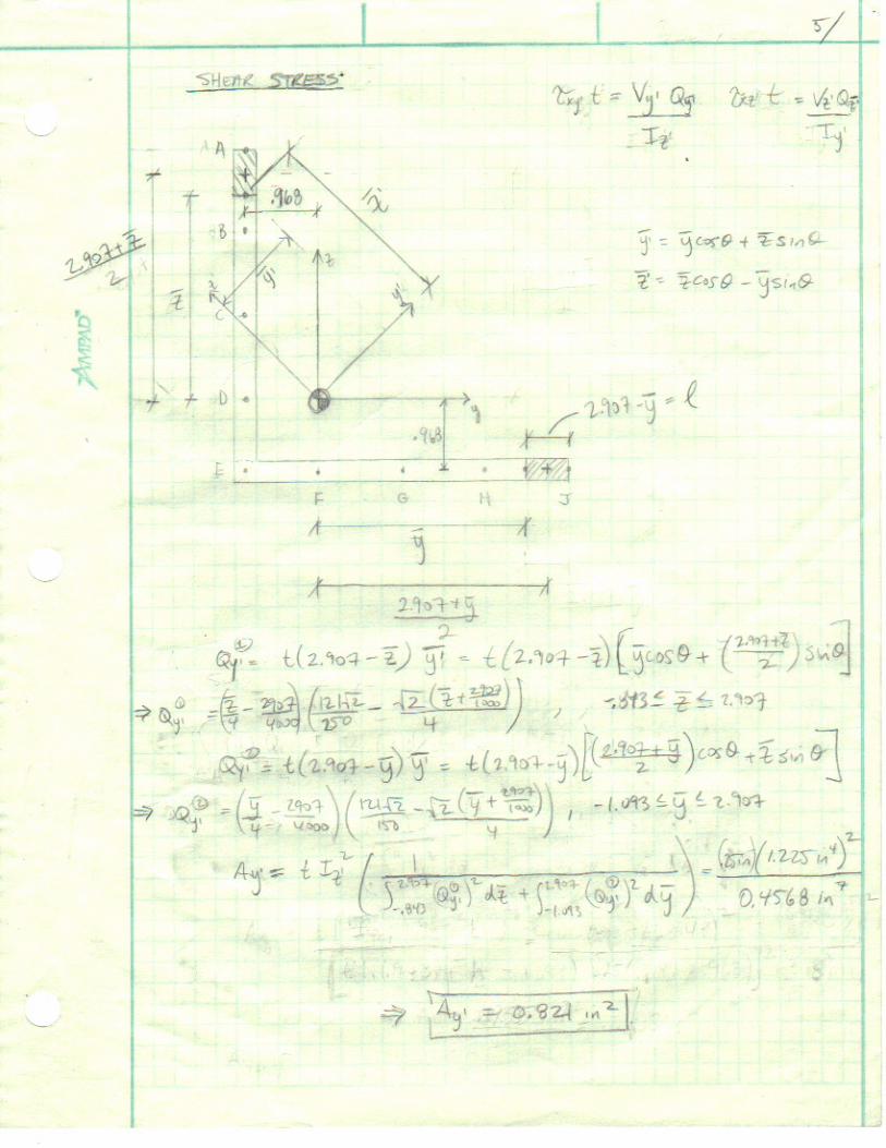
SHEAR STRESS

For a principal coordinate system, shear flow is given by

𝜏𝜏𝜏𝜏 =𝑉𝑉𝑦𝑦′𝑄𝑄𝑧𝑧′𝐼𝐼𝑧𝑧′

+𝑉𝑉𝑧𝑧′𝑄𝑄𝑦𝑦′𝐼𝐼𝑦𝑦′

The equations for 𝑄𝑄𝑦𝑦′ and 𝑄𝑄𝑧𝑧′ were computed for each rectangle of the cross section in MATLAB, see Appendix C.

Vertical leg

𝑄𝑄𝑦𝑦′ = �𝑧𝑧̅4−

29074000

� �121√2

250−√2�𝑧𝑧̿ + 2907

1000� �4

� ,−.843 ≤ 𝑧𝑧̅ ≤ 2.907

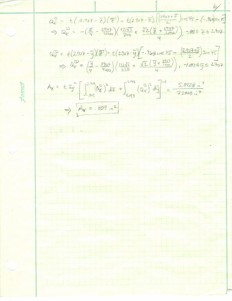
𝑄𝑄𝑧𝑧′ = −�𝑧𝑧̅4−

29074000

� �121√2

250+√2�𝑧𝑧̿ + 2907

1000� �4

� ,−.843 ≤ 𝑧𝑧̅ ≤ 2.907

Horizontal leg

𝑄𝑄𝑦𝑦′ = �𝑦𝑦�4−

29074000

� �121√2

250−√2�𝑦𝑦� + 2907

1000� �4

� ,−1.093 ≤ 𝑦𝑦� ≤ 2.907

A

C

B

D E

𝒛𝒛

𝒚𝒚

PAGE 5

𝑄𝑄𝑧𝑧′ = �𝑦𝑦�4−

29074000

� �121√2

250+√2�𝑦𝑦� + 2907

1000� �4

� ,−1.093 ≤ 𝑦𝑦� ≤ 2.907

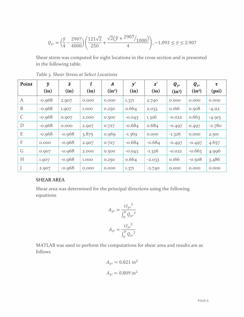
Shear stress was computed for eight locations in the cross section and is presented in the following table.

Table 3. Shear Stress at Select Locations

Point 𝒚𝒚� (in)

𝒛𝒛� (in)

𝒍𝒍 (in)

𝑨𝑨 (in2)

𝒚𝒚′ (in)

𝒛𝒛′ (in)

𝑸𝑸𝒚𝒚′ (in3)

𝑸𝑸𝒛𝒛′ (in3)

𝝉𝝉 (psi)

A -0.968 2.907 0.000 0.000 1.371 2.740 0.000 0.000 0.000

B -0.968 1.907 1.000 0.250 0.664 2.033 0.166 0.508 -4.112

C -0.968 0.907 2.000 0.500 -0.043 1.326 -0.022 0.663 -4.915

D -0.968 0.000 2.907 0.727 -0.684 0.684 -0.497 0.497 -2.780

E -0.968 -0.968 3.875 0.969 -1.369 0.000 -1.326 0.000 2.501

F 0.000 -0.968 2.907 0.727 -0.684 -0.684 -0.497 -0.497 4.657

G 0.907 -0.968 2.000 0.500 -0.043 -1.326 -0.022 -0.663 4.996

H 1.907 -0.968 1.000 0.250 0.664 -2.033 0.166 -0.508 3.486

J 2.907 -0.968 0.000 0.000 1.371 -2.740 0.000 0.000 0.000

SHEAR AREA

Shear area was determined for the principal directions using the following equations

𝐴𝐴𝑦𝑦′ =𝜏𝜏𝐼𝐼𝑦𝑦′2

∫ 𝑄𝑄𝑦𝑦′2𝑏𝑏𝑎𝑎

𝐴𝐴𝑧𝑧′ =𝜏𝜏𝐼𝐼𝑧𝑧′2

∫ 𝑄𝑄𝑧𝑧′2𝑏𝑏𝑎𝑎

MATLAB was used to perform the computations for shear area and results are as follows

𝐴𝐴𝑦𝑦′ = 0.821 in2

𝐴𝐴𝑧𝑧′ = 0.809 in2

PAGE 6

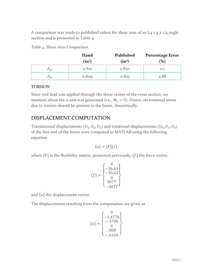
A comparison was made to published values for shear area of an L4 x 4 x 1/4 angle section and is presented in Table 4.

Table 4. Shear Area Comparison

Hand (in2)

Published (in2)

Percentage Error (%)

𝐴𝐴𝑦𝑦′ 0.821 0.820 0.1

𝐴𝐴𝑧𝑧′ 0.809 0.833 2.88

TORSION

Since end load was applied through the shear center of the cross section, no moment about the x-axis was generated (i.e., 𝑀𝑀1 = 0). Hence, no torsional stress due to torsion should be present in the beam, theoretically.

DISPLACEMENT COMPUTATION Translational displacements (𝑈𝑈1,𝑈𝑈2,𝑈𝑈3) and rotational displacements (𝑈𝑈4,𝑈𝑈5,𝑈𝑈6) of the free end of the beam were computed in MATLAB using the following equation

{𝑢𝑢} = [𝐹𝐹]{𝑓𝑓}

where [𝐹𝐹] is the flexibility matrix, presented previously, {𝑓𝑓} the force vector,

{𝑓𝑓} =

⎩⎪⎨

⎪⎧

0−36.63−36.63

03077−3077⎭

⎪⎬

⎪⎫

and {𝑢𝑢} the displacement vector.

The displacements resulting from the computation are given as

{𝑢𝑢} =

⎩⎪⎨

⎪⎧

0−1.4778−.3736

0. 008−.0316 ⎭

⎪⎬

⎪⎫

PAGE 7

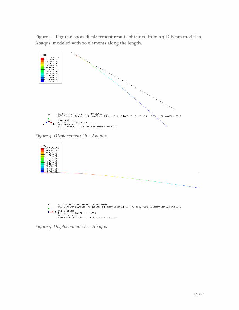
Figure 4 - Figure 6 show displacement results obtained from a 3-D beam model in Abaqus, modeled with 20 elements along the length.

Figure 4. Displacement U1 – Abaqus

Figure 5. Displacement U2 – Abaqus

PAGE 8

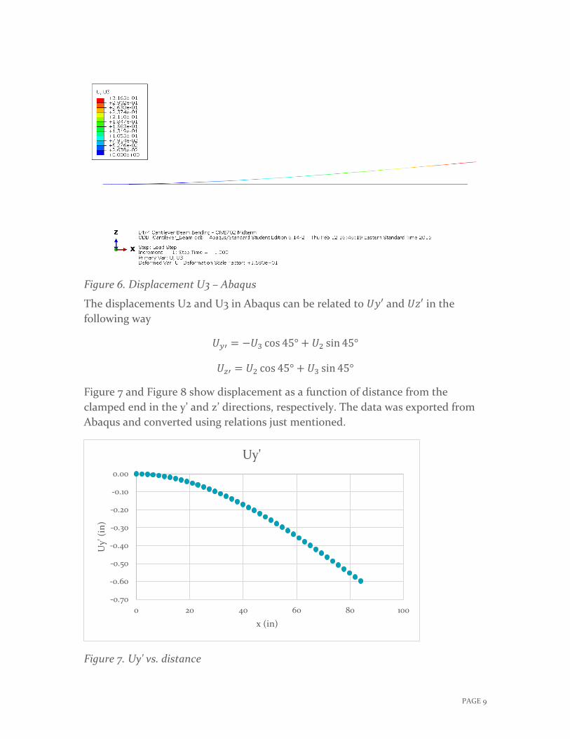
Figure 6. Displacement U3 – Abaqus

The displacements U2 and U3 in Abaqus can be related to 𝑈𝑈𝑦𝑦′ and 𝑈𝑈𝑧𝑧′ in the following way

𝑈𝑈𝑦𝑦′ = −𝑈𝑈3 cos 45° + 𝑈𝑈2 sin 45°

𝑈𝑈𝑧𝑧′ = 𝑈𝑈2 cos 45° + 𝑈𝑈3 sin 45°

Figure 7 and Figure 8 show displacement as a function of distance from the clamped end in the y’ and z’ directions, respectively. The data was exported from Abaqus and converted using relations just mentioned.

Figure 7. Uy' vs. distance

-0.70

-0.60

-0.50

-0.40

-0.30

-0.20

-0.10

0.00

0 20 40 60 80 100

Uy'

(in)

x (in)

Uy'

PAGE 9

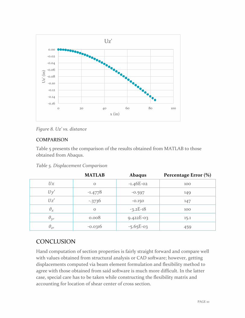
Figure 8. Uz' vs. distance

COMPARISON

Table 5 presents the comparison of the results obtained from MATLAB to those obtained from Abaqus.

Table 5. Displacement Comparison

MATLAB Abaqus Percentage Error (%)

𝑈𝑈𝑈𝑈 0 -1.46E-02 100

𝑈𝑈𝑦𝑦′ -1.4778 -0.597 149

𝑈𝑈𝑧𝑧′ -.3736 -0.150 147

𝜗𝜗𝑥𝑥 0 -3.2E-18 100

𝜗𝜗𝑦𝑦′ 0.008 9.422E-03 15.1

𝜗𝜗𝑧𝑧′ -0.0316 -5.65E-03 459

CONCLUSION Hand computation of section properties is fairly straight forward and compare well with values obtained from structural analysis or CAD software; however, getting displacements computed via beam element formulation and flexibility method to agree with those obtained from said software is much more difficult. In the latter case, special care has to be taken while constructing the flexibility matrix and accounting for location of shear center of cross section.

-0.16

-0.14

-0.12

-0.10

-0.08

-0.06

-0.04

-0.02

0.00

0 20 40 60 80 100

Uz'

(in)

x (in)

Uz'

PAGE 10

Appendix A

1

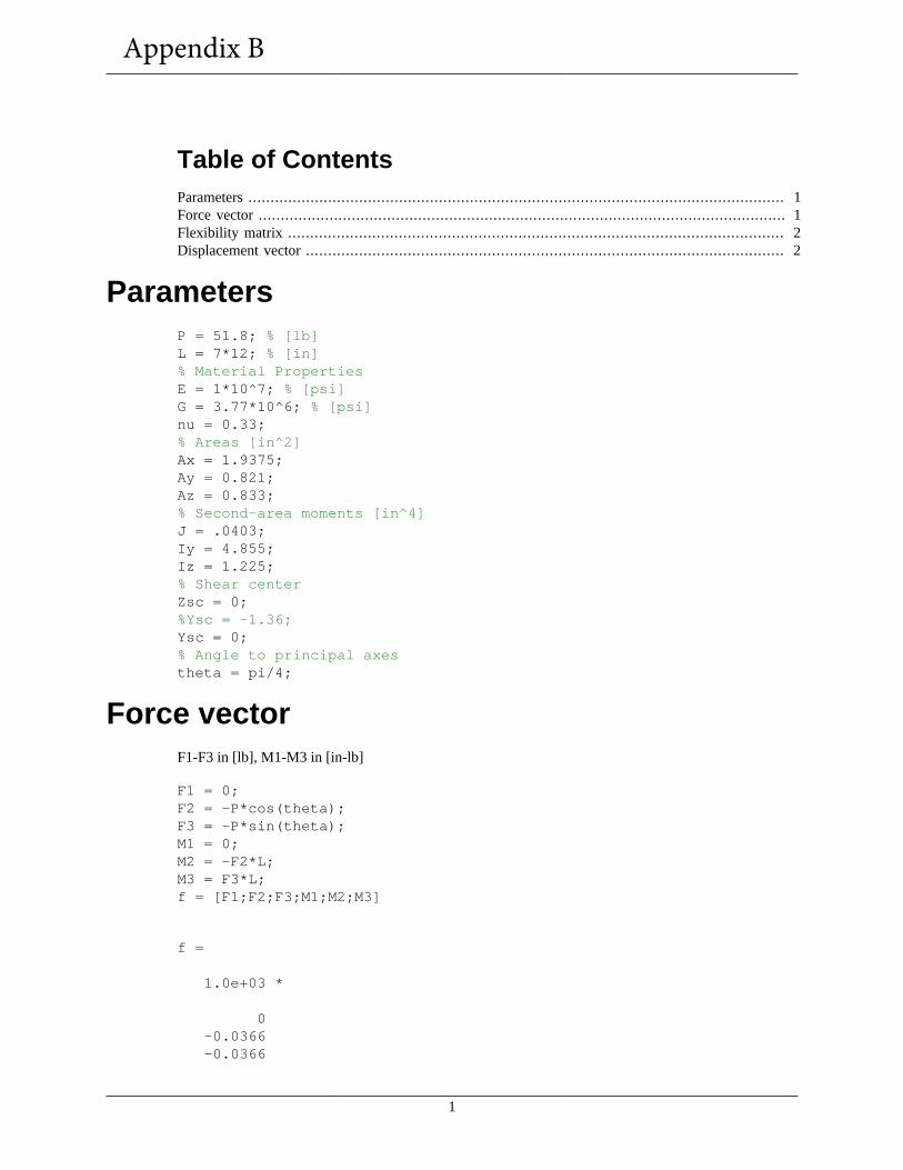
Table of ContentsParameters ......................................................................................................................... 1Force vector ....................................................................................................................... 1Flexibility matrix ................................................................................................................ 2Displacement vector ............................................................................................................ 2

ParametersP = 51.8; % [lb]L = 7*12; % [in]% Material PropertiesE = 1*10^7; % [psi]G = 3.77*10^6; % [psi]nu = 0.33;% Areas [in^2]Ax = 1.9375;Ay = 0.821;Az = 0.833;% Second-area moments [in^4]J = .0403;Iy = 4.855;Iz = 1.225;% Shear centerZsc = 0;%Ysc = -1.36;Ysc = 0;% Angle to principal axestheta = pi/4;

Force vectorF1-F3 in [lb], M1-M3 in [in-lb]

F1 = 0;F2 = -P*cos(theta);F3 = -P*sin(theta);M1 = 0;M2 = -F2*L;M3 = F3*L;f = [F1;F2;F3;M1;M2;M3]

f =

1.0e+03 *

0 -0.0366 -0.0366

Appendix B

2

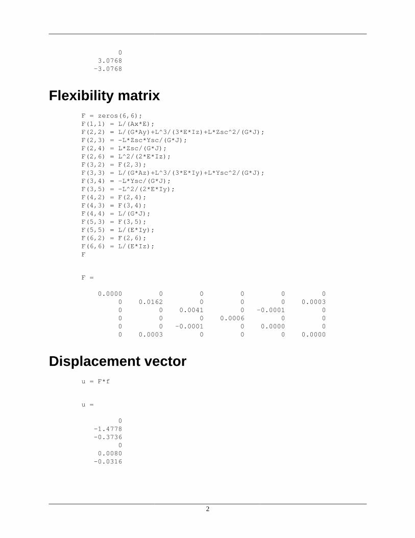
0 3.0768 -3.0768

Flexibility matrixF = zeros(6,6);F(1,1) = L/(Ax*E);F(2,2) = L/(G*Ay)+L^3/(3*E*Iz)+L*Zsc^2/(G*J);F(2,3) = -L*Zsc*Ysc/(G*J);F(2,4) = L*Zsc/(G*J);F(2,6) = L^2/(2*E*Iz);F(3,2) = F(2,3);F(3,3) = L/(G*Az)+L^3/(3*E*Iy)+L*Ysc^2/(G*J);F(3,4) = -L*Ysc/(G*J);F(3,5) = -L^2/(2*E*Iy);F(4,2) = F(2,4);F(4,3) = F(3,4);F(4,4) = L/(G*J);F(5,3) = F(3,5);F(5,5) = L/(E*Iy);F(6,2) = F(2,6);F(6,6) = L/(E*Iz);F

F =

0.0000 0 0 0 0 00 0.0162 0 0 0 0.00030 0 0.0041 0 -0.0001 00 0 0 0.0006 0 00 0 -0.0001 0 0.0000 00 0.0003 0 0 0 0.0000

Displacement vectoru = F*f

u =

0 -1.4778 -0.3736

0 0.0080 -0.0316

1

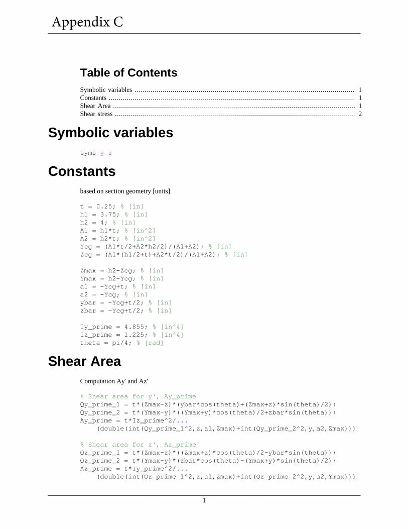
Table of ContentsSymbolic variables .............................................................................................................. 1Constants ........................................................................................................................... 1Shear Area ......................................................................................................................... 1Shear stress ........................................................................................................................ 2

Symbolic variablessyms y z

Constantsbased on section geometry [units]

t = 0.25; % [in]h1 = 3.75; % [in]h2 = 4; % [in]A1 = h1*t; % [in^2]A2 = h2*t; % [in^2]Ycg = (A1*t/2+A2*h2/2)/(A1+A2); % [in]Zcg = (A1*(h1/2+t)+A2*t/2)/(A1+A2); % [in]

Zmax = h2-Zcg; % [in]Ymax = h2-Ycg; % [in]a1 = -Ycg+t; % [in]a2 = -Ycg; % [in]ybar = -Ycg+t/2; % [in]zbar = -Ycg+t/2; % [in]

Iy_prime = 4.855; % [in^4]Iz_prime = 1.225; % [in^4]theta = pi/4; % [rad]

Shear AreaComputation Ay' and Az'

% Shear area for y', Ay_primeQy_prime_1 = t*(Zmax-z)*(ybar*cos(theta)+(Zmax+z)*sin(theta)/2);Qy_prime_2 = t*(Ymax-y)*((Ymax+y)*cos(theta)/2+zbar*sin(theta));Ay_prime = t*Iz_prime^2/... (double(int(Qy_prime_1^2,z,a1,Zmax)+int(Qy_prime_2^2,y,a2,Zmax)))

% Shear area for z', Az_primeQz_prime_1 = t*(Zmax-z)*((Zmax+z)*cos(theta)/2-ybar*sin(theta));Qz_prime_2 = t*(Ymax-y)*(zbar*cos(theta)-(Ymax+y)*sin(theta)/2);Az_prime = t*Iy_prime^2/... (double(int(Qz_prime_1^2,z,a1,Zmax)+int(Qz_prime_2^2,y,a2,Ymax)))

Appendix C

2

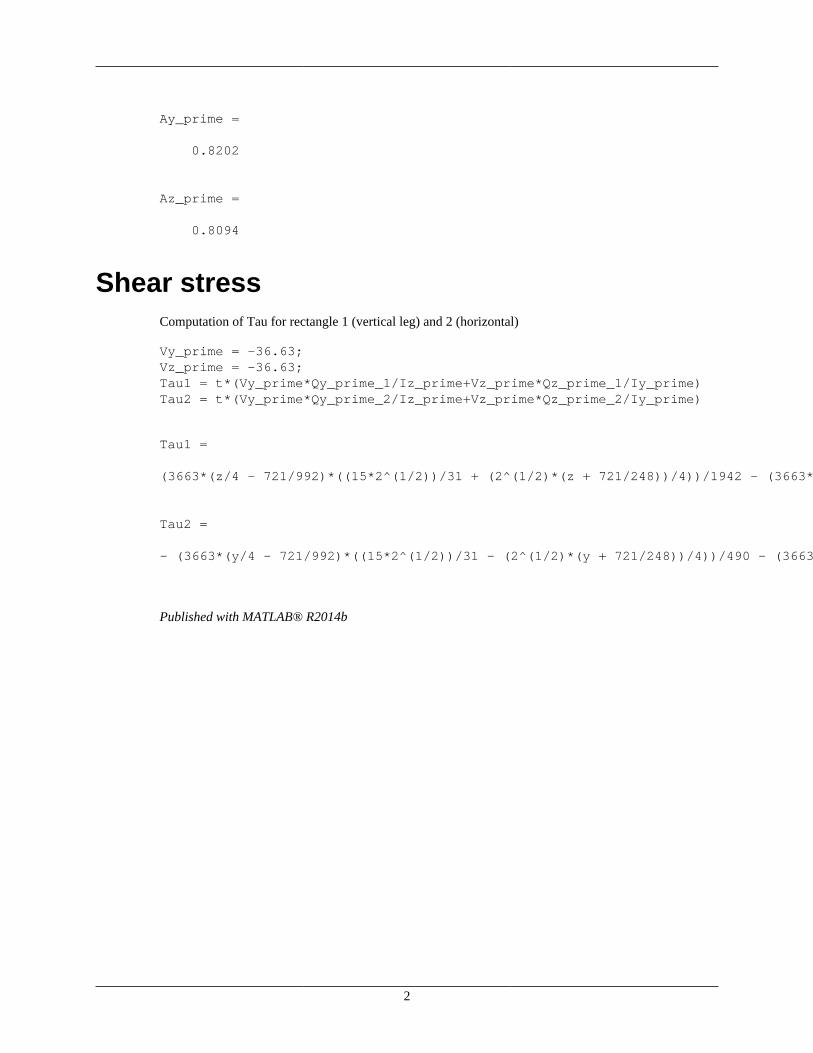
Ay_prime =

0.8202

Az_prime =

0.8094

Shear stressComputation of Tau for rectangle 1 (vertical leg) and 2 (horizontal)

Vy_prime = -36.63;Vz_prime = -36.63;Tau1 = t*(Vy_prime*Qy_prime_1/Iz_prime+Vz_prime*Qz_prime_1/Iy_prime)Tau2 = t*(Vy_prime*Qy_prime_2/Iz_prime+Vz_prime*Qz_prime_2/Iy_prime)

Tau1 = (3663*(z/4 - 721/992)*((15*2^(1/2))/31 + (2^(1/2)*(z + 721/248))/4))/1942 - (3663*(z/4 - 721/992)*((15*2^(1/2))/31 - (2^(1/2)*(z + 721/248))/4))/490 Tau2 = - (3663*(y/4 - 721/992)*((15*2^(1/2))/31 - (2^(1/2)*(y + 721/248))/4))/490 - (3663*(y/4 - 721/992)*((15*2^(1/2))/31 + (2^(1/2)*(y + 721/248))/4))/1942

Published with MATLAB® R2014b