Water Distribution Network for the Municipality of Barrhead, Alberta

Proposal Submitted by Hydrofour

Zoe Martiniak (260446300) Reid Hadaway (260518382)

Diane Kim (260462152) Svetlana Zdanovich (260482402)

April 6th, 2016

CIVE 421 Municipal Systems McGill University

Presented to Dr. Ronald Gehr

i

Abstract The primary objective of this report is to design a water distribution system to service the Town

of Barrhead, Alberta for a 20-year period. A population of 6295 was forecasted for the year 2036

using the exponential method. The designed water distribution system will supply the demands

of residential, commercial, and industrial sectors and the water demand per sector was calculated

based on existing and future developments in the town. Paddle River, which runs across the

south end of the town, was chosen as the water source. The intake location was determined based

on a calculated intake depth of 1.18 m. The critical fire flow was predicted to occur at the

Barrhead Healthcare Centre, close to the school district, and would require a total fire flow of

6750 L/min for a duration of 2 hours. Two storage units, a ground reservoir and an elevated

reservoir, were designed. The elevated reservoir, located across the industrial sector north of the

town, will provide the equalizing, fire, and emergency storages. The ground reservoir, attached

to the water treatment plant and located south of the town, will supply the average and maximum

daily flows. The water distribution network was designed using AquaCAD. Five scenarios were

modeled including average day, minimum hours, maximum hour, maximum day, and maximum

day + fire. The network was designed with respect to pressure limitations and minimal head

losses. The selected pipe sizes are: 200 mm, 300 mm and 480 mm. The pumping system, which

includes two continuously operating pumps in parallel and a third backup diesel pump, was

designed based on the required pressures of the network.

ii

Acknowledgements

We at HydroFour would like to graciously thank Professor Ronald Gehr along with Sarah El

Outayek, Angela Huston, and Martine Lavallée for their support and instruction throughout the

preparation and completion of this project and report.

iii

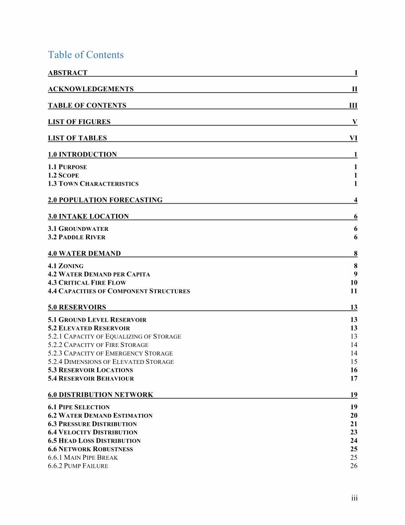
Table of Contents ABSTRACT I

ACKNOWLEDGEMENTS II

TABLE OF CONTENTS III

LIST OF FIGURES V

LIST OF TABLES VI

1.0 INTRODUCTION 11.1 PURPOSE 11.2 SCOPE 11.3 TOWN CHARACTERISTICS 1

2.0 POPULATION FORECASTING 4

3.0 INTAKE LOCATION 63.1 GROUNDWATER 63.2 PADDLE RIVER 6

4.0 WATER DEMAND 84.1 ZONING 84.2 WATER DEMAND PER CAPITA 94.3 CRITICAL FIRE FLOW 104.4 CAPACITIES OF COMPONENT STRUCTURES 11

5.0 RESERVOIRS 135.1 GROUND LEVEL RESERVOIR 135.2 ELEVATED RESERVOIR 135.2.1 CAPACITY OF EQUALIZING OF STORAGE 135.2.2 CAPACITY OF FIRE STORAGE 145.2.3 CAPACITY OF EMERGENCY STORAGE 145.2.4 DIMENSIONS OF ELEVATED STORAGE 155.3 RESERVOIR LOCATIONS 165.4 RESERVOIR BEHAVIOUR 17

6.0 DISTRIBUTION NETWORK 196.1 PIPE SELECTION 196.2 WATER DEMAND ESTIMATION 206.3 PRESSURE DISTRIBUTION 216.4 VELOCITY DISTRIBUTION 236.5 HEAD LOSS DISTRIBUTION 246.6 NETWORK ROBUSTNESS 256.6.1 MAIN PIPE BREAK 256.6.2 PUMP FAILURE 26

iv

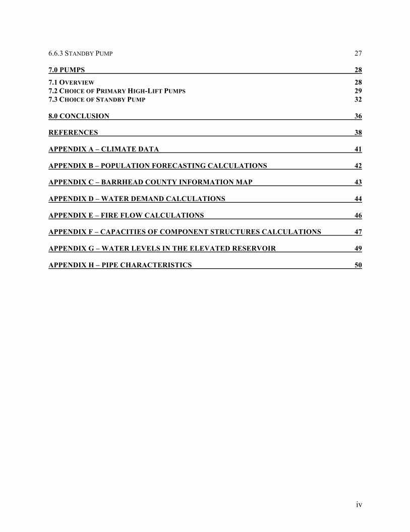
6.6.3 STANDBY PUMP 27

7.0 PUMPS 287.1 OVERVIEW 287.2 CHOICE OF PRIMARY HIGH-LIFT PUMPS 297.3 CHOICE OF STANDBY PUMP 32

8.0 CONCLUSION 36

REFERENCES 38

APPENDIX A – CLIMATE DATA 41

APPENDIX B – POPULATION FORECASTING CALCULATIONS 42

APPENDIX C – BARRHEAD COUNTY INFORMATION MAP 43

APPENDIX D – WATER DEMAND CALCULATIONS 44

APPENDIX E – FIRE FLOW CALCULATIONS 46

APPENDIX F – CAPACITIES OF COMPONENT STRUCTURES CALCULATIONS 47

APPENDIX G – WATER LEVELS IN THE ELEVATED RESERVOIR 49

APPENDIX H – PIPE CHARACTERISTICS 50

v

List of Figures Figure 1 – Map of Barrhead, AB (Google Maps, 2016) ................................................................. 2Figure 2 – Topography of Barrhead, AB (Toporama, 2016) .......................................................... 2Figure 3 – Barrhead Projected Population ...................................................................................... 5Figure 4 - Intake Location in the Paddle River (Google Maps, 2016) ........................................... 7Figure 5 – Barrhead Zoning Map .................................................................................................... 8Figure 6 – Simplified Schematic of the Water Distribution System of Barrhead ........................ 11Figure 7 – Equalizing Storage Mass Diagram .............................................................................. 14Figure 8 – Elevation View of the Elevated Reservoir .................................................................. 15Figure 9 – Plan View of the Elevated Reservoir ........................................................................... 16Figure 10 – Locations of Ground and Elevated Reservoirs (Town of Barrhead, 2016) ............... 17Figure 11 – Proposed Water Distribution Network ...................................................................... 20Figure 12 – Pressure Distribution at Nodes for Average Day Simulation .................................... 22Figure 13 – Distribution Pressures ................................................................................................ 23Figure 14 – Main Pipe Break ........................................................................................................ 25Figure 15 – Pump Failure ............................................................................................................. 26Figure 16 - Distribution of Pressures During a Standby Pump Scenario ..................................... 27Figure 17 - Parallel Arrangement of Pumps (Integrated Publishing Inc., 2016) .......................... 28Figure 18 – Primary Pump Characteristic Curve and Operating Point ......................................... 30Figure 19 – Two Identical Parallel Pumps' Operating Point ........................................................ 32Figure 20 – Standby Pump Characteristic Curve and Operating Point ........................................ 33Figure 21 – Pressure Distribution Under Maximum Day + Fire Flows, Standby Pump Alone ... 35Figure 22 – Barrhead Climate Data (ACIS, 2016) ....................................................................... 41Figure 23 – Barrhead County Information Map (Town of Barrhead, 2016) ................................ 43

vi

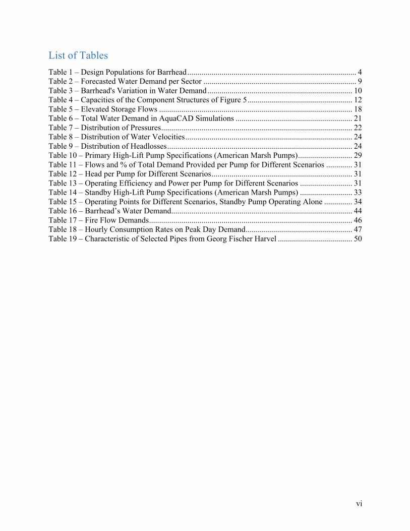
List of Tables Table 1 – Design Populations for Barrhead .................................................................................... 4Table 2 – Forecasted Water Demand per Sector ............................................................................ 9Table 3 – Barrhead's Variation in Water Demand ........................................................................ 10Table 4 – Capacities of the Component Structures of Figure 5 .................................................... 12Table 5 – Elevated Storage Flows ................................................................................................ 18Table 6 – Total Water Demand in AquaCAD Simulations .......................................................... 21Table 7 – Distribution of Pressures ............................................................................................... 22Table 8 – Distribution of Water Velocities ................................................................................... 24Table 9 – Distribution of Headlosses ............................................................................................ 24Table 10 – Primary High-Lift Pump Specifications (American Marsh Pumps) ........................... 29Table 11 – Flows and % of Total Demand Provided per Pump for Different Scenarios ............. 31Table 12 – Head per Pump for Different Scenarios ...................................................................... 31Table 13 – Operating Efficiency and Power per Pump for Different Scenarios .......................... 31Table 14 – Standby High-Lift Pump Specifications (American Marsh Pumps) .......................... 33Table 15 – Operating Points for Different Scenarios, Standby Pump Operating Alone .............. 34Table 16 – Barrhead’s Water Demand .......................................................................................... 44Table 17 – Fire Flow Demands ..................................................................................................... 46Table 18 – Hourly Consumption Rates on Peak Day Demand ..................................................... 47Table 19 – Characteristic of Selected Pipes from Georg Fischer Harvel ..................................... 50

1

1.0 Introduction

1.1 Purpose

The purpose of this project is to design a water distribution system for the town of Barrhead,

Alberta that is capable of meeting the current and projected water demand for a 20-year period.

The longevity of the designed system is based on the life expectancy of the PVC pipe, which is

typically 20 years.

1.2 Scope

This report documents the process of designing a water distribution system for the town of

Barrhead. The distribution network will provide water for residential, commercial, and industrial

uses, and will ensure that adequate flows can be provided during emergencies. The design

process is based on the following:

• Population forecasting

• Intake location

• Evaluation of component structure capacities

• Design of storage

• Design of distribution network

• Evaluation of pumps

1.3 Town Characteristics

Located 120 km Northwest of Edmonton, Barrhead has an overall area of 8.10 km2 with a

slightly varying elevation around 640m (Figure 1 and Figure 2) (CityData, 2016). The town has a

humid continental climate with typically warm summers and cold winters. Due to its high

altitude and close proximity to the Rocky Mountains, warm, dry chinook winds can greatly

increase the temperature during the winter months. The detailed climatic data is of Barrhead can

be found in Appendix A. Barrhead’s landscape consists of boreal forest and natural sand hill

while being close in proximity to the Athabasca, Pembina and Paddle river (Hydrogeological

consultants Ltd, 1998). The Paddle River, which runs across the town, will act as the water

source for the water distribution network.

2

Figure 1 – Map of Barrhead, AB (Google Maps, 2016)

Figure 2 – Topography of Barrhead, AB (Toporama, 2016)

Barrhead, Alberta is a town with a population of 4432 and is expected to have a current

population of 4542 (Statistics Canada, 2012). Despite its small population size, Barrhead is home

3

to a golf course, campground, several healthcare centers, multiple community facilities, and

commercial businesses. Schools in Barrhead include the Barrhead Elementary School, Barrhead

Composite High School, and the Vista Virtual school (Town of Barrhead, 2016).

The main sources of industry that support Barrhead’s economy are oil and gas, forestry and

agriculture. Regarding the regional industry, agriculture is of major importance to the Barrhead

economy. They pride themselves on their highly competitive hog operations and cattle feedlots.

The town of Barrhead serves as the regional trading and service center for the County of

Barrhead and the surrounding area, which services over 500 businesses in the region (Alberta

Community Profiles, 2016). Some of the manufactured products in the county of Barrhead

include animal feeds, chemicals and herbicides, concrete, fertilizers, and many more.

In terms of non-domestic development, the municipality of Barrhead has proposed for the

construction of the Barrhead Regional Aquatics Centre. This will greatly increase the amount of

water that the town will need and will have to be accounted for in the calculations for the water

distribution network.

4

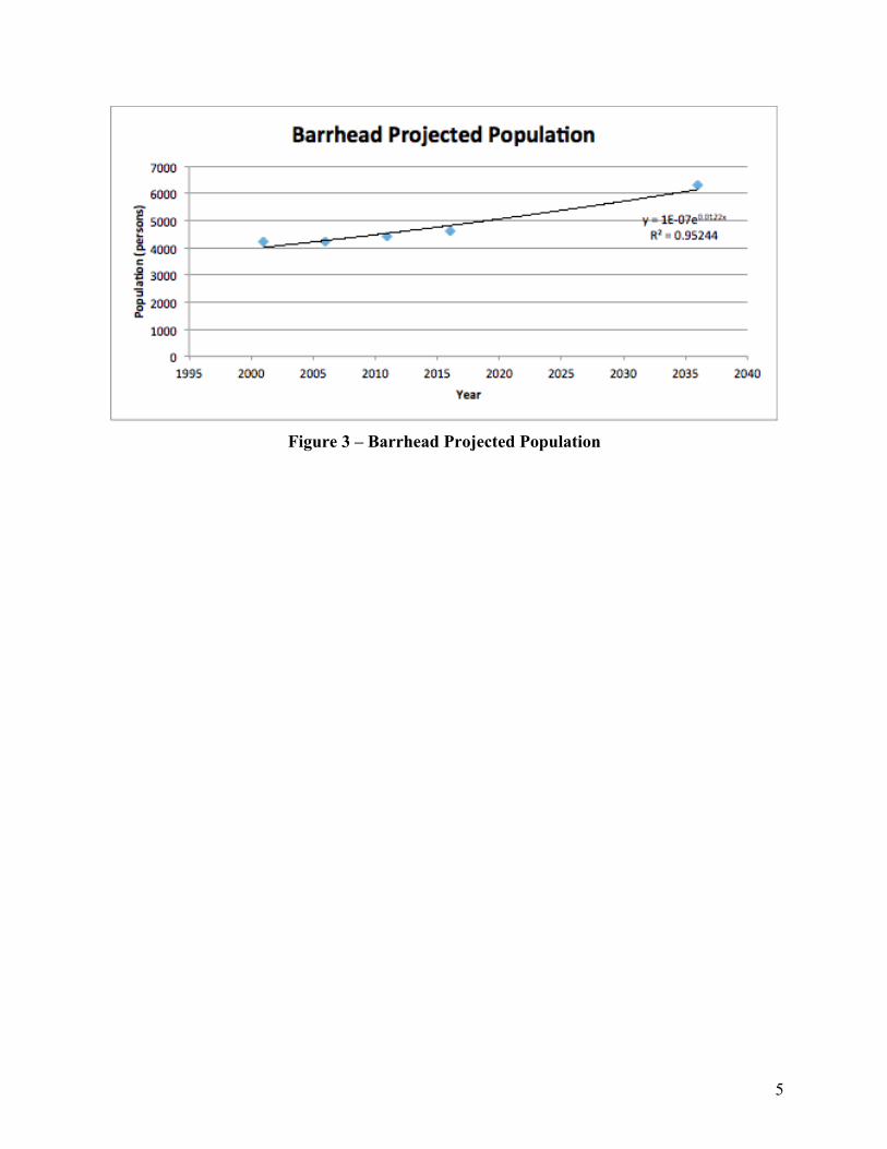
2.0 Population Forecasting The population of Barrhead was 4,432 in 2011, according to the Canadian census of population

in Alberta (Statistics Canada, 2012). Assuming exponential growth, the current population in

2016 is 4,618 people and is projected to be 6,295 people in 2036 (Figure 3). Detailed

calculations can be found on Appendix B. In the recent months, Alberta has been experiencing a

sizeable amount of lay-offs in the oil and gas industry. However, with the current federal

government investing in renewable energy coupled with worker-led initiatives such as Iron &

Earth, who aims to retrain electricians from the oilsand sector to install solar panels, there is a

new niche market to be exploited (Lazzrino, 2016). This trend will retain current population and

potentially attract more skilled workers in smaller towns. Barrhead is planning two large housing

expansion projects that allow for accommodation for this future population growth, as well as

potentially welcome more population to settle in Barrhead. These housing expansion projects are

the Hillcrest Home and Beaver Brooke Estates, which are located at points 23 and 24 on the

Barrhead County information map in Appendix C.

Using the Exponential Method (with an acceptable R2 of 0.95244), we determine the current and

future population as indicated in Table 1.

Table 1 – Design Populations for Barrhead

Year 2001 2006 2011 2016* 2036*

Population 4213 4209 4432 4618 6295

*Projected using exponential method. (Source: Statistics Canada, 2012)

5

Figure 3 – Barrhead Projected Population

6

3.0 Intake Location

3.1 Groundwater

According to the Alberta Ministry of Environment and Sustainable Resource Development,

water level map, the static groundwater level in the wet well located near the proposed water

treatment plant is 5.5 m (Gov. of Alberta, 2016). Although the depth is not too problematic,

pumping from the aquifer would incur additional costs related to pipes, excavation work, and

pumps. For these reasons, groundwater was not considered as an intake source.

3.2 Paddle River

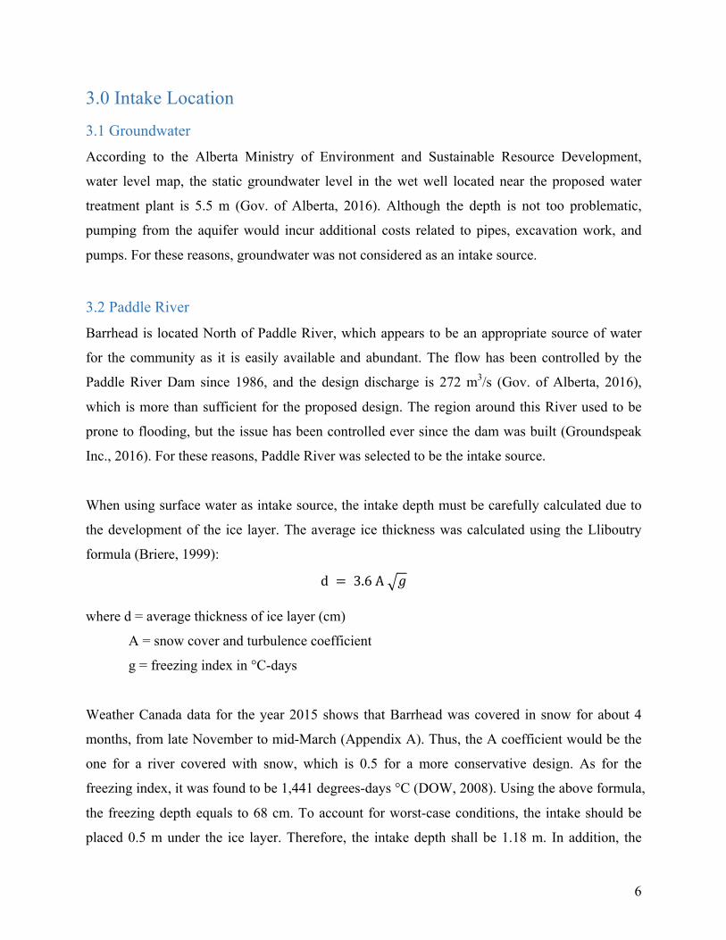
Barrhead is located North of Paddle River, which appears to be an appropriate source of water

for the community as it is easily available and abundant. The flow has been controlled by the

Paddle River Dam since 1986, and the design discharge is 272 m3/s (Gov. of Alberta, 2016),

which is more than sufficient for the proposed design. The region around this River used to be

prone to flooding, but the issue has been controlled ever since the dam was built (Groundspeak

Inc., 2016). For these reasons, Paddle River was selected to be the intake source.

When using surface water as intake source, the intake depth must be carefully calculated due to

the development of the ice layer. The average ice thickness was calculated using the Lliboutry

formula (Briere, 1999):

d = 3.6A 𝑔

where d = average thickness of ice layer (cm)

A = snow cover and turbulence coefficient

g = freezing index in °C-days

Weather Canada data for the year 2015 shows that Barrhead was covered in snow for about 4

months, from late November to mid-March (Appendix A). Thus, the A coefficient would be the

one for a river covered with snow, which is 0.5 for a more conservative design. As for the

freezing index, it was found to be 1,441 degrees-days °C (DOW, 2008). Using the above formula,

the freezing depth equals to 68 cm. To account for worst-case conditions, the intake should be

placed 0.5 m under the ice layer. Therefore, the intake depth shall be 1.18 m. In addition, the

7

intake should have a clearance of 1 m from the river bed to avoid debris being sucked in.

Consequently, the intake location needs to be at a point where the depth of the river is more than

2.18 m. Figure 4 gives an approximation of the intake location.

Figure 4 - Intake Location in the Paddle River (Google Maps, 2016)

8

4.0 Water Demand

4.1 Zoning

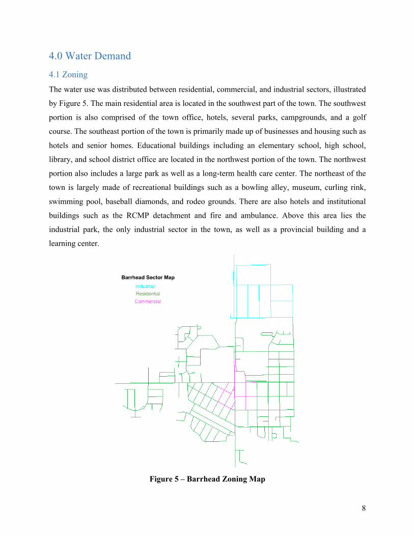
The water use was distributed between residential, commercial, and industrial sectors, illustrated

by Figure 5. The main residential area is located in the southwest part of the town. The southwest

portion is also comprised of the town office, hotels, several parks, campgrounds, and a golf

course. The southeast portion of the town is primarily made up of businesses and housing such as

hotels and senior homes. Educational buildings including an elementary school, high school,

library, and school district office are located in the northwest portion of the town. The northwest

portion also includes a large park as well as a long-term health care center. The northeast of the

town is largely made of recreational buildings such as a bowling alley, museum, curling rink,

swimming pool, baseball diamonds, and rodeo grounds. There are also hotels and institutional

buildings such as the RCMP detachment and fire and ambulance. Above this area lies the

industrial park, the only industrial sector in the town, as well as a provincial building and a

learning center.

Figure 5 – Barrhead Zoning Map

9

4.2 Water Demand per Capita

The average daily water demand was calculated from the sum of water demand per building type

in the town of Barrhead, accounting for future developments such as the Hillcrest Home and

Beaver Brooke Estates projects as well as the Barrhead Regional Aquatic Centre project. The

EPA recommended design flows were used in calculating the average daily water demand

(Shammas and Wang, 2011). Appendix D summarizes the applied design flows for every

building in Barrhead. Table 2 summarizes the water demand per sector. The final water use per

capita is 0.8681 m3/day.

Table 2 – Forecasted Water Demand per Sector

Consumption

(%)

Water Use

(m3/day/capita)

Total residential consumption 67.13 0.5827

Total commercial consumption 7.90 0.2253

Total Industrial Park 6.93 0.0601

Total - 0.8681

Peak factors (Shammas and Wang, 2011) were used to account for the variations in water

demand in modeling four demand scenarios for the town of Barrhead. The results are

summarized in Table 3.

10

Table 3 – Barrhead's Variation in Water Demand

Average Daily

Flow (m3/day)

Max Daily Flow

(m3/day)

Max Hourly

Flow (m3/day)

Min hourly Flow

(m3/day)

Peak Factor 1 2 3 0.5

Adjusted Total

Water Use per

Capita

0.8681 1.736 2.604 0.4341

Total

Residential

3668 7337 11010 1834

Total

Commercial

432 863 1295 216

Total Industrial 379 379 379 379

Total 5465 8579 12680 2428

The Barrhead water distribution system must be designed to accommodate for the maximum

hourly flow of 12,680 m3/day.

4.3 Critical Fire Flow

The fire flow is designed for critical locations which are home to valuable assets or value. In this

case, the Barrhead Healthcare Centre was chosen due to its close proximity to the school and

commercial districts. Additionally, the healthcare centre is one of the most important buildings in

the community in terms of medical treatment as there are few clinics in the town. Alternative

critical and highly dense locations such as the school district and the Agrena & Swimming Pool

were also considered. Although the Agrena & Swimming Pool is the largest community services

facility, capable of accommodating a large number of people, it was considered less critical when

compared to the healthcare centre which sits facing the school district.

The Barrhead Healthcare Centre is an ordinary one story building mainly constructed from brick

and masonry walls with a total area of 4800 m2 according to the Healthcare Centre. Also, the

11

Healthcare Centre is 25 m away from a small supply building. Detailed calculations can be found

in Appendix E.

The critical fire flow was found to be:

𝐹 = 6750𝐿/𝑚𝑖𝑛

4.4 Capacities of Component Structures

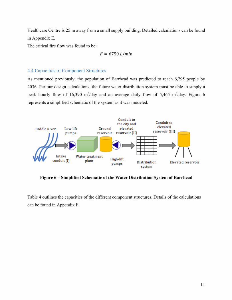
As mentioned previously, the population of Barrhead was predicted to reach 6,295 people by

2036. Per our design calculations, the future water distribution system must be able to supply a

peak hourly flow of 16,390 m3/day and an average daily flow of 5,465 m3/day. Figure 6

represents a simplified schematic of the system as it was modeled.

Figure 6 – Simplified Schematic of the Water Distribution System of Barrhead

Table 4 outlines the capacities of the different component structures. Details of the calculations

can be found in Appendix F.

12

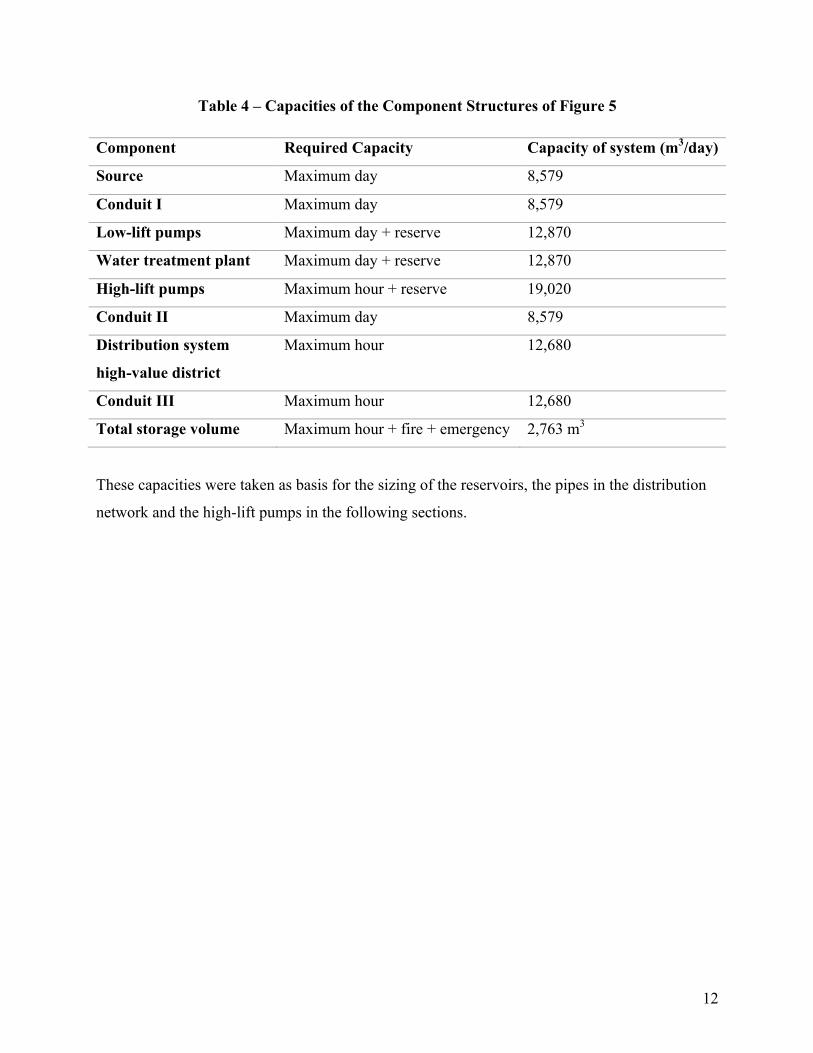
Table 4 – Capacities of the Component Structures of Figure 5

Component Required Capacity Capacity of system (m3/day)

Source Maximum day 8,579

Conduit I Maximum day 8,579

Low-lift pumps Maximum day + reserve 12,870

Water treatment plant Maximum day + reserve 12,870

High-lift pumps Maximum hour + reserve 19,020

Conduit II Maximum day 8,579

Distribution system

high-value district

Maximum hour 12,680

Conduit III Maximum hour 12,680

Total storage volume Maximum hour + fire + emergency 2,763 m3

These capacities were taken as basis for the sizing of the reservoirs, the pipes in the distribution

network and the high-lift pumps in the following sections.

13

5.0 Reservoirs

5.1 Ground Level Reservoir

The ground level reservoir will be located at the water treatment plant. Water pumped from the

river will undergo purification and treatment before being stored in the ground level storage

which is to be located at the water treatment plant. The ground level reservoir will supply the

average and maximum daily flows to the distribution network. This reservoir is designed to store

10,930 m3 of water, the double the average daily flow anticipated by the network.

𝑉𝑜𝑙𝑢𝑚𝑒𝑜𝑓𝐺𝑟𝑜𝑢𝑛𝑑𝑆𝑡𝑜𝑟𝑎𝑔𝑒 = 2 𝐴𝑣𝑔𝐷𝑎𝑖𝑙𝑦𝐶𝑜𝑛𝑠𝑢𝑚𝑝𝑡𝑖𝑜𝑛 = 2 ∗ 5,465𝑚I = 10,930𝑚I

5.2 Elevated Reservoir

The elevated reservoirs will provide for equalizing, fire, and emergency conditions. The

equalizing storage ensures the water supply during the peak hours of the day while fire and

emergency storage will ensure supply in case of emergencies such as fires or failures in the water

mains. From summing the equalizing, fire, and emergency storages, the elevated reservoir for the

town of Barrhead must have a minimum volume of 2,763 m3. Taking into account 0.8 meters for

overfill and for additional emergency capacity, our design volume is 2,808 m3. The calculations

and detailed descriptions of the equalizing, fire, and emergency storages are found in Appendix F

and the following sections 5.2.1, 5.2.2, and 5.2.3, respectively.

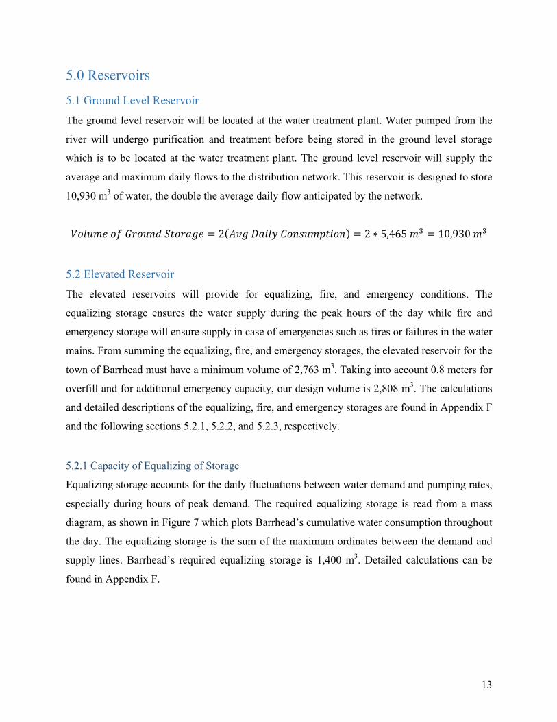
5.2.1 Capacity of Equalizing of Storage

Equalizing storage accounts for the daily fluctuations between water demand and pumping rates,

especially during hours of peak demand. The required equalizing storage is read from a mass

diagram, as shown in Figure 7 which plots Barrhead’s cumulative water consumption throughout

the day. The equalizing storage is the sum of the maximum ordinates between the demand and

supply lines. Barrhead’s required equalizing storage is 1,400 m3. Detailed calculations can be

found in Appendix F.

14

Figure 7 – Equalizing Storage Mass Diagram

5.2.2 Capacity of Fire Storage

According to the Fire Underwriters Survey performed by CGI Risk Management Services for the

Canadian Insurance industry, the minimal required duration of fire flow is 2 hours for a

population of 6, 295 (CGI Group Inc, 1999). The critical fire demand was calculated to be 6750

L/min in section 4.3. Based on this information, the required fire storage was calculated to be

810 m3. Detailed calculations can be found in Appendix F.

5.2.3 Capacity of Emergency Storage

The emergency storage accounts for 25% of the sum of the fire and equalizing storage. The

required emergency storage was found to be 552.5 m3. Detailed calculations can be found in

Appendix F.

15

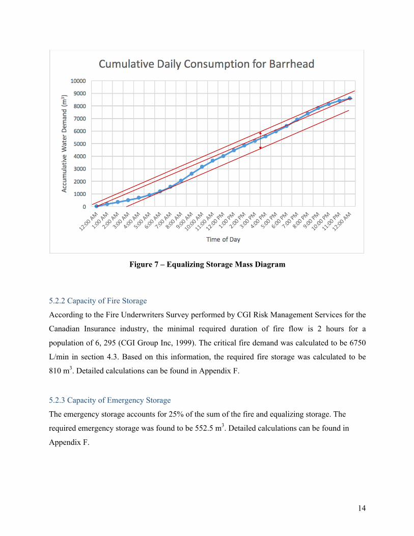
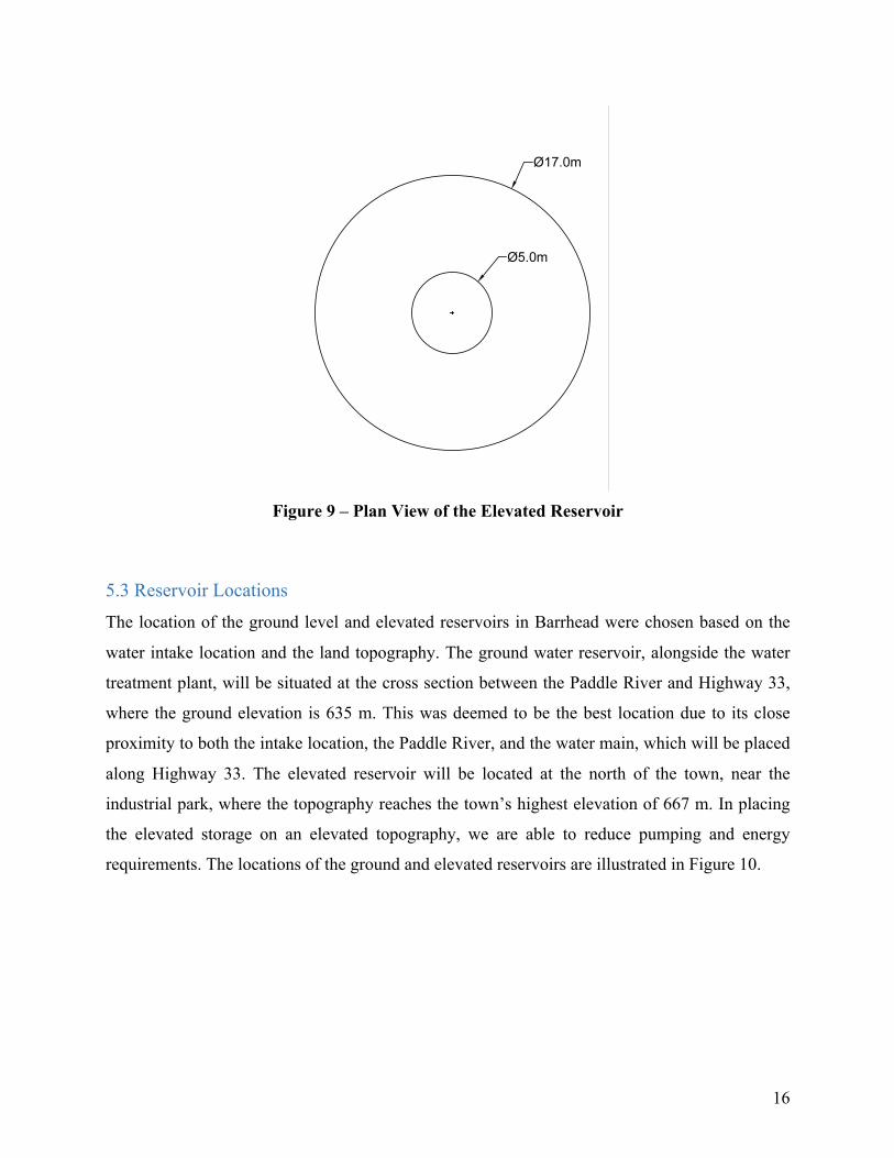
5.2.4 Dimensions of Elevated Storage

The water tower will be situated beyond the town’s load center since the area provides high

elevations and since this setup will decrease the required head by the pumps. The AquaCAD

simulation has shown that the water in the tower will reach a maximum height of 22 m. An

additional 0.8 m will be added to the actual height of the tower to accommodate overfilling. The

water tower will be comprised of a cylindrical reservoir atop of a cylindrical column. The

minimum required elevated reservoir volume of 2,763 m3 will be split among the two cylindrical

structures. The suggested design dimensions are illustrated in Figures 8 and 9 below. The

cylindrical column will hold a volume of 295 m3 while the cylindrical reservoir will hold a

volume of 2513 m3, for a total volume of 2808 m3.

Figure 8 – Elevation View of the Elevated Reservoir

16

Figure 9 – Plan View of the Elevated Reservoir

5.3 Reservoir Locations

The location of the ground level and elevated reservoirs in Barrhead were chosen based on the

water intake location and the land topography. The ground water reservoir, alongside the water

treatment plant, will be situated at the cross section between the Paddle River and Highway 33,

where the ground elevation is 635 m. This was deemed to be the best location due to its close

proximity to both the intake location, the Paddle River, and the water main, which will be placed

along Highway 33. The elevated reservoir will be located at the north of the town, near the

industrial park, where the topography reaches the town’s highest elevation of 667 m. In placing

the elevated storage on an elevated topography, we are able to reduce pumping and energy

requirements. The locations of the ground and elevated reservoirs are illustrated in Figure 10.

17

Figure 10 – Locations of Ground and Elevated Reservoirs (Town of Barrhead, 2016)

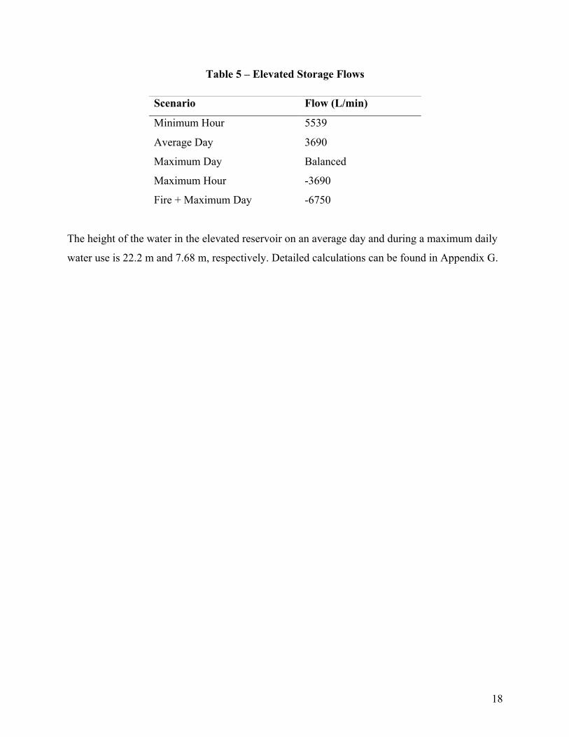
5.4 Reservoir Behaviour

The flows of the elevated storage under various scenarios are outlined in Table 5 below, as

determined by AquaCAD. It should be noted that negatives flows represent the emptying of the

elevated reservoir.

18

Table 5 – Elevated Storage Flows

Scenario Flow (L/min)

Minimum Hour 5539

Average Day 3690

Maximum Day Balanced

Maximum Hour -3690

Fire + Maximum Day -6750

The height of the water in the elevated reservoir on an average day and during a maximum daily

water use is 22.2 m and 7.68 m, respectively. Detailed calculations can be found in Appendix G.

19

6.0 Distribution Network

6.1 Pipe Selection

The pipe network distribution is designed to lay underneath the road base of Barrhead to increase

ease of access to the pipes for maintenance or repair. However, some pipes were added that do

not lie directly under the road in order to avoid dead-ends and loops. A closed-loop system is

ideal for reducing head losses and allow for adequate distribution of water to meet the city's

water demands.

PVC was chosen as the pipe material, since PVC is generally preferred over metal pipes for

water distribution. Using metal pipes for water distribution can introduce dissolved metals into

the drinking water supply as a result of corrosion. PVC also has a higher Hazen-Williams

coefficient, which relates to a lower friction factor and therefore reduced head losses. The

Hazen-Williams coefficient for PVC pipes are usually around 150, however for design purposes

we have selected a Hazen-Williams coefficient of 140 for our hydraulic simulations. PVC pipes

are commercially available as schedule 40 or schedule 80. The main differences between these

schedules are the pipe thickness and the pressure rating. Schedule 80 pipes have thicker walls but

are more resistant ion, replacement to internal and external pressures. In order to prolong the

lifetime of the piping network and avoid pipe leaks, schedule 80 pumps are the optimal choice.

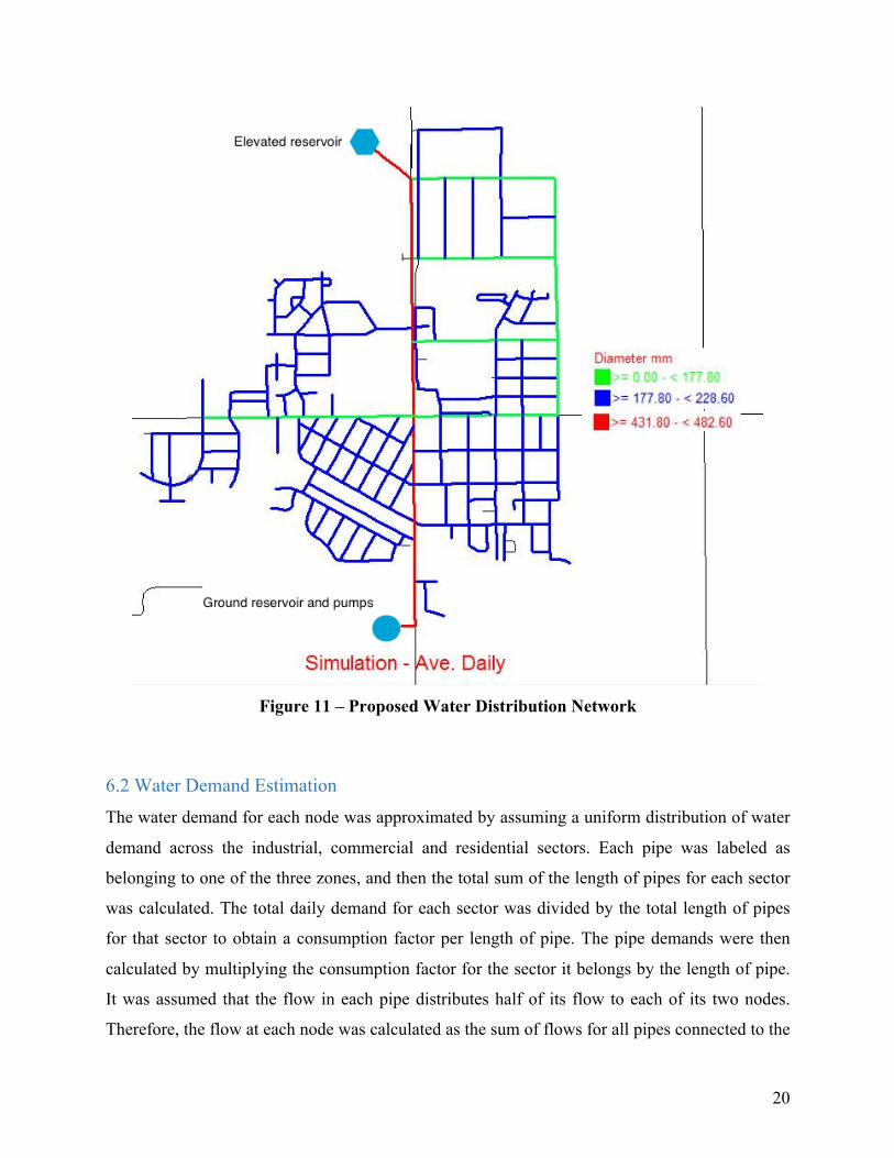
The layout of the primary, secondary and distribution mains are indicated in Figure 11. It was

decided that decided to maintain consistent sizing for each of the three types of water distribution

pipes to avoid construction and replacement issues, as well as reduce overall costs. The pipe

sizing was optimized for efficient distribution for average day, as well as all other simulations.

This was done by considering pressures and head losses throughout the distribution. The selected

pipe sizes are summarized in Appendix H. The nominal pipe diameters of 200 mm, 300 mm and

480 mm were selected for the water distribution, secondary and primary water main pipes,

respectively.

20

Figure 11 – Proposed Water Distribution Network

6.2 Water Demand Estimation

The water demand for each node was approximated by assuming a uniform distribution of water

demand across the industrial, commercial and residential sectors. Each pipe was labeled as

belonging to one of the three zones, and then the total sum of the length of pipes for each sector

was calculated. The total daily demand for each sector was divided by the total length of pipes

for that sector to obtain a consumption factor per length of pipe. The pipe demands were then

calculated by multiplying the consumption factor for the sector it belongs by the length of pipe.

It was assumed that the flow in each pipe distributes half of its flow to each of its two nodes.

Therefore, the flow at each node was calculated as the sum of flows for all pipes connected to the

21

node, divided by two. This method of consumption approximation is appropriate for Barrhead,

since the population density is relatively uniform throughout the residential sector, and the

commercial sector is centrally located along the water main. The total demand for each

simulation is summarized in Table 6.

Table 6 – Total Water Demand in AquaCAD Simulations

Average day

(L/min)

Max day

(L/min)

Max day +

fire (L/min)

Peak hour

(L/min)

Min Hour

(L/min)

Residential 2402 4803 4803 7205 1201

Commercial 966.2 1932 1932 2899 483.1

Industrial 345.9 345.9 345.9 345.9 345.9

Fire 0.00 0.00 6750 0.00 0.00

Total 3714 7081 13830 10450 2030

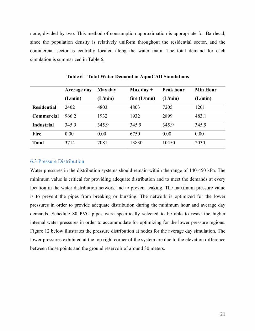
6.3 Pressure Distribution

Water pressures in the distribution systems should remain within the range of 140-450 kPa. The

minimum value is critical for providing adequate distribution and to meet the demands at every

location in the water distribution network and to prevent leaking. The maximum pressure value

is to prevent the pipes from breaking or bursting. The network is optimized for the lower

pressures in order to provide adequate distribution during the minimum hour and average day

demands. Schedule 80 PVC pipes were specifically selected to be able to resist the higher

internal water pressures in order to accommodate for optimizing for the lower pressure regions.

Figure 12 below illustrates the pressure distribution at nodes for the average day simulation. The

lower pressures exhibited at the top right corner of the system are due to the elevation difference

between those points and the ground reservoir of around 30 meters.

22

Figure 12 – Pressure Distribution at Nodes for Average Day Simulation

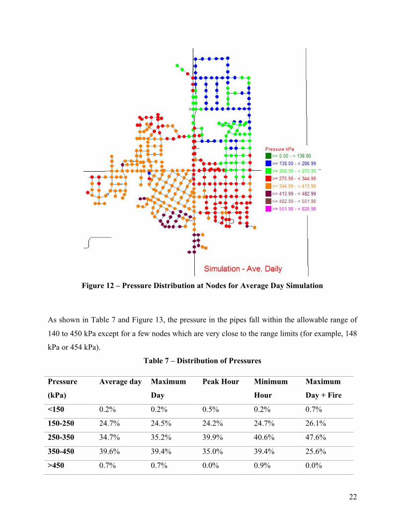
As shown in Table 7 and Figure 13, the pressure in the pipes fall within the allowable range of

140 to 450 kPa except for a few nodes which are very close to the range limits (for example, 148

kPa or 454 kPa).

Table 7 – Distribution of Pressures

Pressure

(kPa)

Average day Maximum

Day

Peak Hour Minimum

Hour

Maximum

Day + Fire

<150 0.2% 0.2% 0.5% 0.2% 0.7%

150-250 24.7% 24.5% 24.2% 24.7% 26.1%

250-350 34.7% 35.2% 39.9% 40.6% 47.6%

350-450 39.6% 39.4% 35.0% 39.4% 25.6%

>450 0.7% 0.7% 0.0% 0.9% 0.0%

23

Figure 13 – Distribution Pressures

6.4 Velocity Distribution

The range for velocities in most water distribution systems in North America is generally 0.6-1.5

m/s. This range ensures that water does not remain stagnant in the piping system, as well as

avoid erosion and abrasion of the pipes. However, in order to maintain adequate pressures within

the system and minimize pumping, the velocities calculated in AquaCAD were below this range.

Therefore, the proposed network operates with lower velocities in order to reduce head losses

and reduce operational costs. As shown in Table 8, the velocities in the pipe network were

usually within the range of 0-0.3 m/s. For the maximum day, 4% of the network operated within

the suggested velocity range.

24

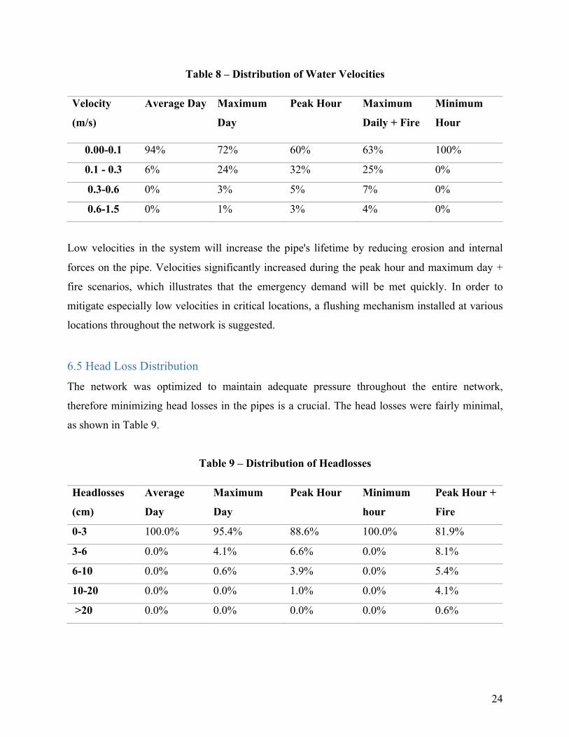
Table 8 – Distribution of Water Velocities

Velocity

(m/s)

Average Day Maximum

Day

Peak Hour Maximum

Daily + Fire

Minimum

Hour

0.00-0.1 94% 72% 60% 63% 100%

0.1 - 0.3 6% 24% 32% 25% 0%

0.3-0.6 0% 3% 5% 7% 0%

0.6-1.5 0% 1% 3% 4% 0%

Low velocities in the system will increase the pipe's lifetime by reducing erosion and internal

forces on the pipe. Velocities significantly increased during the peak hour and maximum day +

fire scenarios, which illustrates that the emergency demand will be met quickly. In order to

mitigate especially low velocities in critical locations, a flushing mechanism installed at various

locations throughout the network is suggested.

6.5 Head Loss Distribution

The network was optimized to maintain adequate pressure throughout the entire network,

therefore minimizing head losses in the pipes is a crucial. The head losses were fairly minimal,

as shown in Table 9.

Table 9 – Distribution of Headlosses

Headlosses

(cm)

Average

Day

Maximum

Day

Peak Hour Minimum

hour

Peak Hour +

Fire

0-3 100.0% 95.4% 88.6% 100.0% 81.9%

3-6 0.0% 4.1% 6.6% 0.0% 8.1%

6-10 0.0% 0.6% 3.9% 0.0% 5.4%

10-20 0.0% 0.0% 1.0% 0.0% 4.1%

>20 0.0% 0.0% 0.0% 0.0% 0.6%

25

6.6 Network Robustness

In order to evaluate the system robustness, three emergency scenarios were considered.

6.6.1 Main Pipe Break

The first emergency scenario considered is failure in one of the primary pipe mains. The system

is tested for a pipe failure between node 129 & 130 broke, which is one of the first pipes that

introduce the flow into the network as illustrated in Figure 14. Therefore, the flow is forced to

travel through smaller distribution pipes. This results in a pressure drop in the rest of the network,

however the distribution of water throughout the majority of the network is still within

acceptable ranges of 138 –359 kPa.

Figure 14 – Main Pipe Break

26

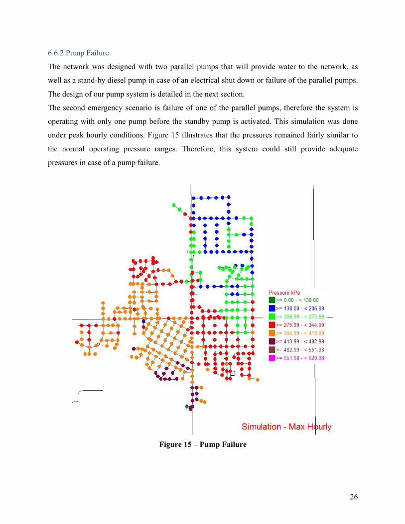
6.6.2 Pump Failure

The network was designed with two parallel pumps that will provide water to the network, as

well as a stand-by diesel pump in case of an electrical shut down or failure of the parallel pumps.

The design of our pump system is detailed in the next section.

The second emergency scenario is failure of one of the parallel pumps, therefore the system is

operating with only one pump before the standby pump is activated. This simulation was done

under peak hourly conditions. Figure 15 illustrates that the pressures remained fairly similar to

the normal operating pressure ranges. Therefore, this system could still provide adequate

pressures in case of a pump failure.

Figure 15 – Pump Failure

27

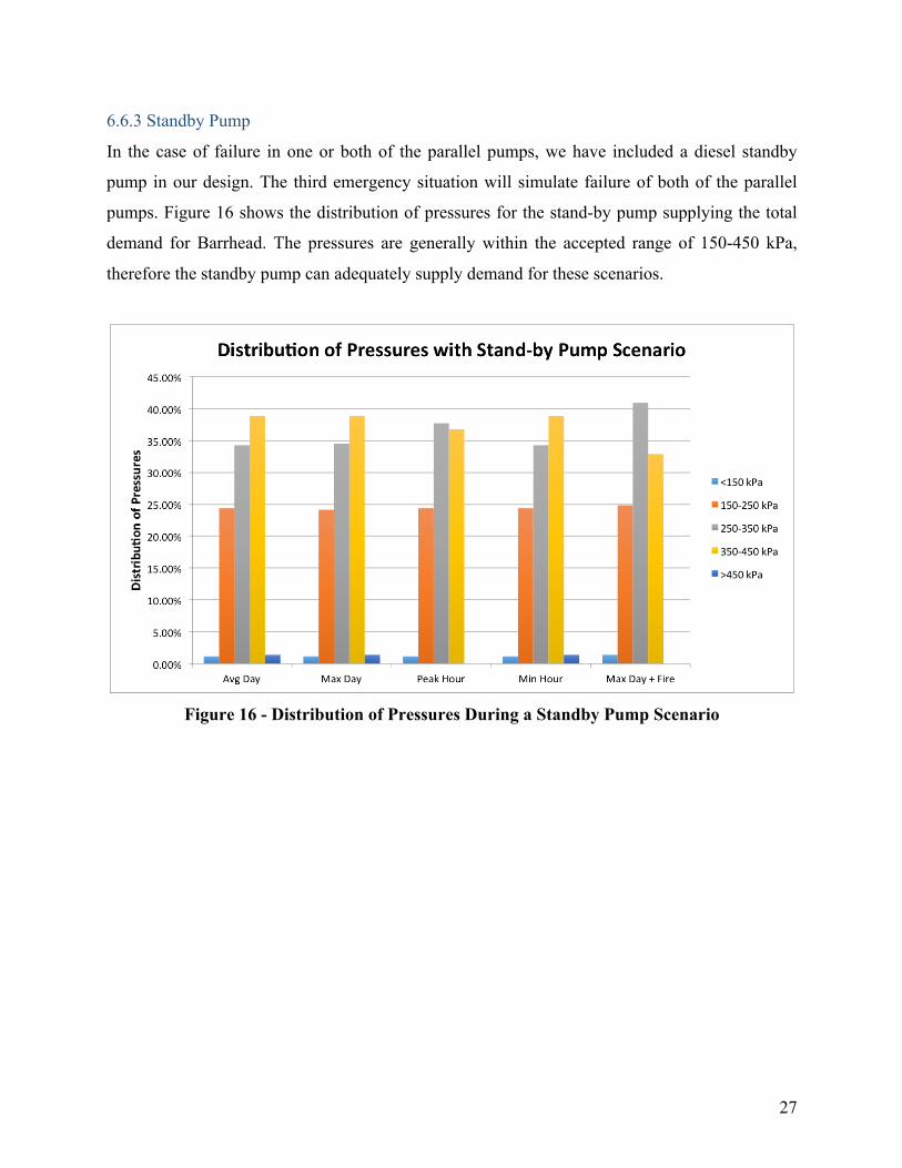
6.6.3 Standby Pump

In the case of failure in one or both of the parallel pumps, we have included a diesel standby

pump in our design. The third emergency situation will simulate failure of both of the parallel

pumps. Figure 16 shows the distribution of pressures for the stand-by pump supplying the total

demand for Barrhead. The pressures are generally within the accepted range of 150-450 kPa,

therefore the standby pump can adequately supply demand for these scenarios.

Figure 16 - Distribution of Pressures During a Standby Pump Scenario

28

7.0 Pumps

7.1 Overview

In order to adequately deliver water from the treatment plant to the town of Barrhead and then to

the elevated reservoir, three high-lift pumps were selected according to the calculated required

capacity and the total pressure of the distribution system. Two identical pumps placed in parallel

at the ground reservoir will operate continuously, each being responsible for supplying half of

the water demand. In addition, a diesel-operated pump will be in standby to cope with

emergencies such as power failures. This third pump will be able to provide the full flow.

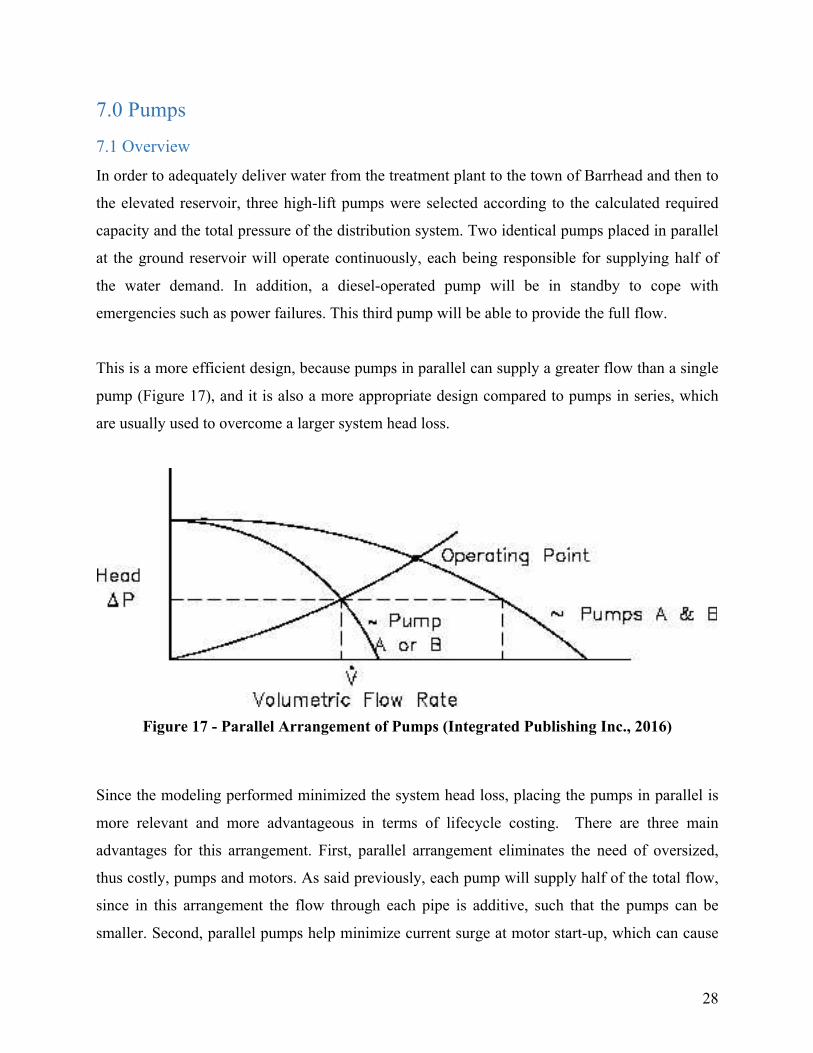
This is a more efficient design, because pumps in parallel can supply a greater flow than a single

pump (Figure 17), and it is also a more appropriate design compared to pumps in series, which

are usually used to overcome a larger system head loss.

Figure 17 - Parallel Arrangement of Pumps (Integrated Publishing Inc., 2016)

Since the modeling performed minimized the system head loss, placing the pumps in parallel is

more relevant and more advantageous in terms of lifecycle costing. There are three main

advantages for this arrangement. First, parallel arrangement eliminates the need of oversized,

thus costly, pumps and motors. As said previously, each pump will supply half of the total flow,

since in this arrangement the flow through each pipe is additive, such that the pumps can be

smaller. Second, parallel pumps help minimize current surge at motor start-up, which can cause

29

problems to the electrical circuit. The use of costly equipment to prevent such damage is

consequently avoided. Last but not least, the water distribution system will be more reliable;

parallel arrangement adds redundancy to the design. If one of the pumps is turned off or fails, the

second one will continue to operate (ITT Industries Inc, 2005).

It is worth noting that pumps usually have a lifespan of 5 years. Since the proposed water

distribution system was designed for a 20-year period, the selected pumps may need replacement

before the end of this design life. Modeling was performed as if pumps were put in place once

the system has achieved its ultimate capacity.

7.2 Choice of Primary High-Lift Pumps

The two high-lift pumps need to provide a flow of 3,795 L/min together, thus each should supply

1,898 L/min. The total system head loss was 46 m during the average daily flow simulation. The

selection of the pumps was maximized based on highest efficiency for the average daily flow

since this is the most frequent scenario. Using the PUMP-FLO centrifugal pump selection

software (Engineered Software Inc, 2016), two identical “American-Marsh Pumps” units were

chosen. Selecting different sizes for the parallel pumps can cause problems, as one pump can

override the second, force closing its check valve, thus potentially leading to a risky situation

(ITT Industries Inc, 2005). For this reason, a safer and simpler route was taken by having

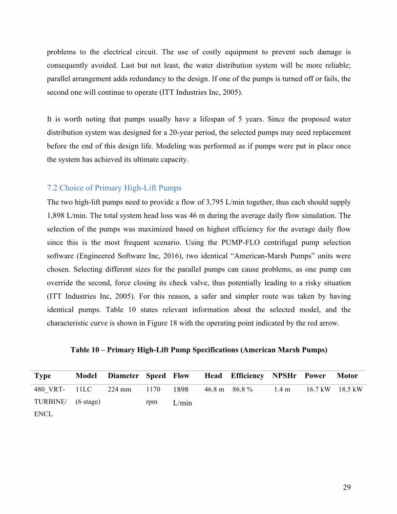
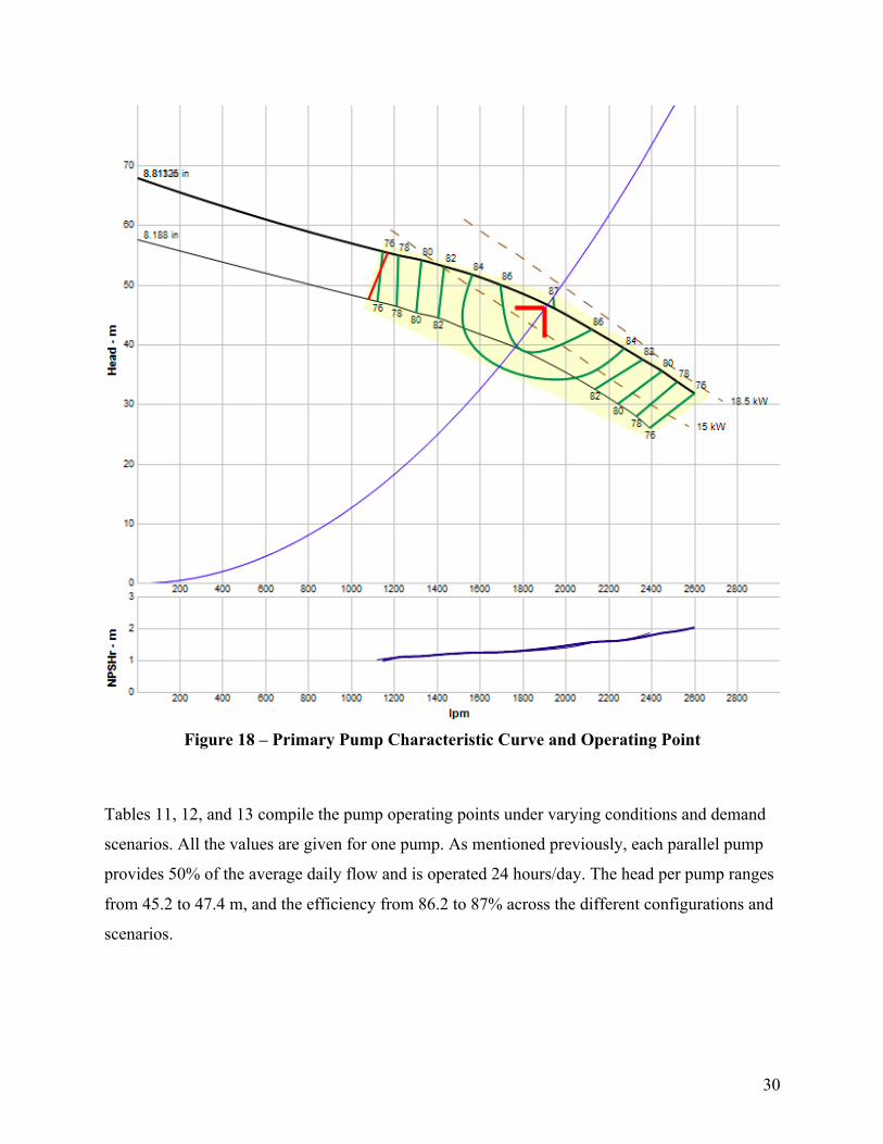
identical pumps. Table 10 states relevant information about the selected model, and the

characteristic curve is shown in Figure 18 with the operating point indicated by the red arrow.

Table 10 – Primary High-Lift Pump Specifications (American Marsh Pumps)

Type Model Diameter Speed Flow Head Efficiency NPSHr Power Motor

480_VRT-

TURBINE/

ENCL

11LC

(6 stage)

224 mm 1170

rpm

1898

L/min

46.8 m 86.8 % 1.4 m 16.7 kW 18.5 kW

30

Figure 18 – Primary Pump Characteristic Curve and Operating Point

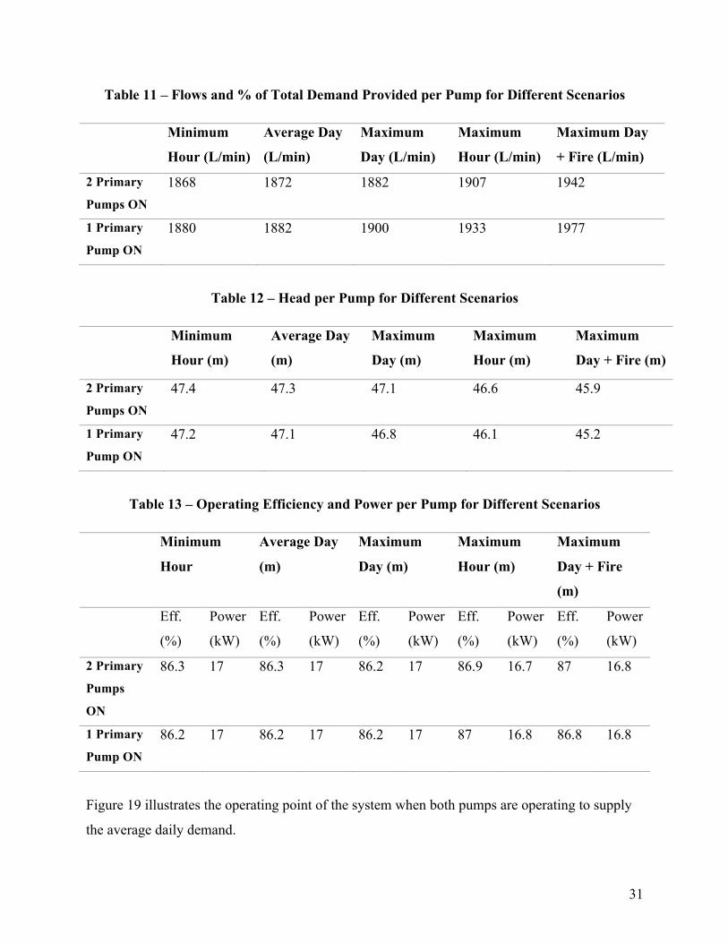
Tables 11, 12, and 13 compile the pump operating points under varying conditions and demand

scenarios. All the values are given for one pump. As mentioned previously, each parallel pump

provides 50% of the average daily flow and is operated 24 hours/day. The head per pump ranges

from 45.2 to 47.4 m, and the efficiency from 86.2 to 87% across the different configurations and

scenarios.

31

Table 11 – Flows and % of Total Demand Provided per Pump for Different Scenarios

Minimum

Hour (L/min)

Average Day

(L/min)

Maximum

Day (L/min)

Maximum

Hour (L/min)

Maximum Day

+ Fire (L/min)

2 Primary

Pumps ON

1868 1872 1882 1907 1942

1 Primary

Pump ON

1880 1882 1900 1933 1977

Table 12 – Head per Pump for Different Scenarios

Minimum

Hour (m)

Average Day

(m)

Maximum

Day (m)

Maximum

Hour (m)

Maximum

Day + Fire (m)

2 Primary

Pumps ON

47.4 47.3 47.1 46.6 45.9

1 Primary

Pump ON

47.2 47.1 46.8 46.1 45.2

Table 13 – Operating Efficiency and Power per Pump for Different Scenarios

Minimum

Hour

Average Day

(m)

Maximum

Day (m)

Maximum

Hour (m)

Maximum

Day + Fire

(m)

Eff.

(%)

Power

(kW)

Eff.

(%)

Power

(kW)

Eff.

(%)

Power

(kW)

Eff.

(%)

Power

(kW)

Eff.

(%)

Power

(kW)

2 Primary

Pumps

ON

86.3 17 86.3 17 86.2 17 86.9 16.7 87 16.8

1 Primary

Pump ON

86.2 17 86.2 17 86.2 17 87 16.8 86.8 16.8

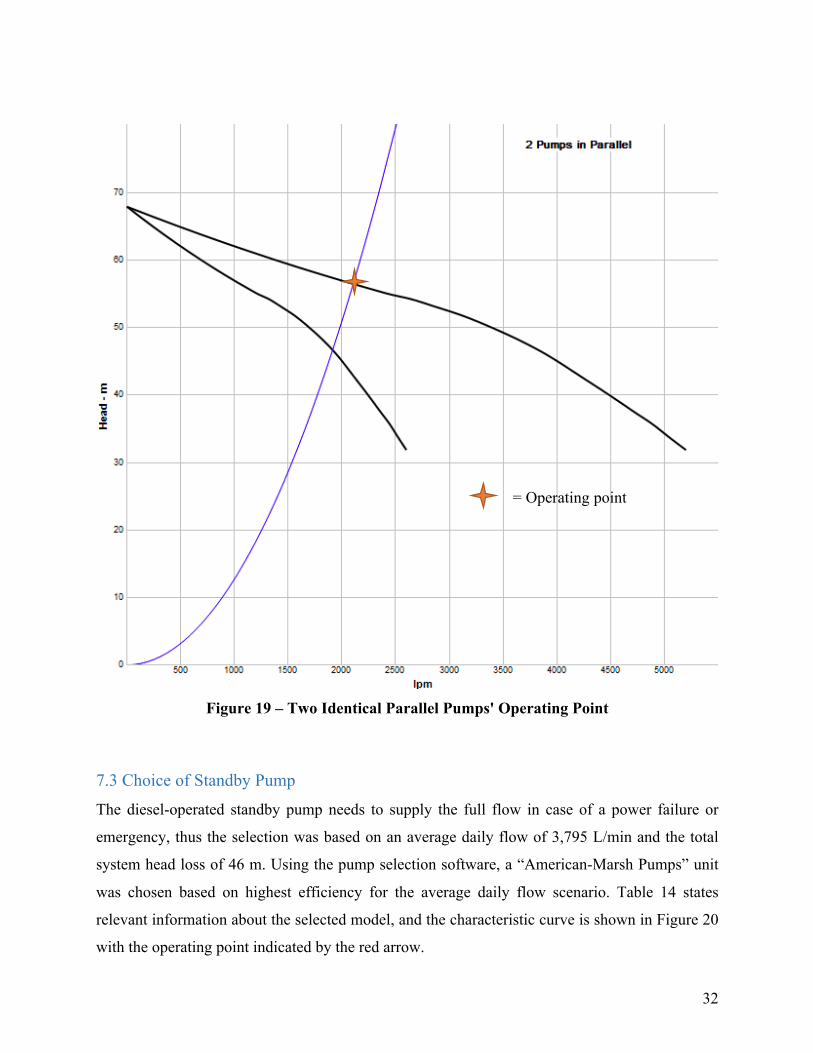
Figure 19 illustrates the operating point of the system when both pumps are operating to supply

the average daily demand.

32

Figure 19 – Two Identical Parallel Pumps' Operating Point

7.3 Choice of Standby Pump

The diesel-operated standby pump needs to supply the full flow in case of a power failure or

emergency, thus the selection was based on an average daily flow of 3,795 L/min and the total

system head loss of 46 m. Using the pump selection software, a “American-Marsh Pumps” unit

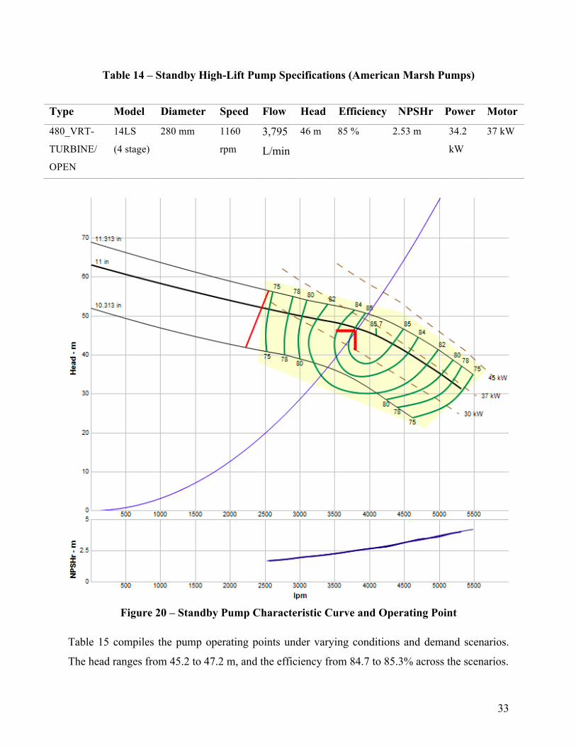
was chosen based on highest efficiency for the average daily flow scenario. Table 14 states

relevant information about the selected model, and the characteristic curve is shown in Figure 20

with the operating point indicated by the red arrow.

= Operating point

33

Table 14 – Standby High-Lift Pump Specifications (American Marsh Pumps)

Figure 20 – Standby Pump Characteristic Curve and Operating Point

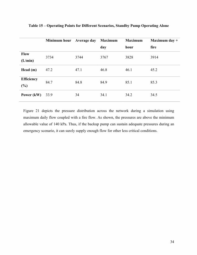
Table 15 compiles the pump operating points under varying conditions and demand scenarios.

The head ranges from 45.2 to 47.2 m, and the efficiency from 84.7 to 85.3% across the scenarios.

Type Model Diameter Speed Flow Head Efficiency NPSHr Power Motor

480_VRT-

TURBINE/

OPEN

14LS

(4 stage)

280 mm 1160

rpm

3,795

L/min

46 m 85 % 2.53 m 34.2

kW

37 kW

34

Table 15 – Operating Points for Different Scenarios, Standby Pump Operating Alone

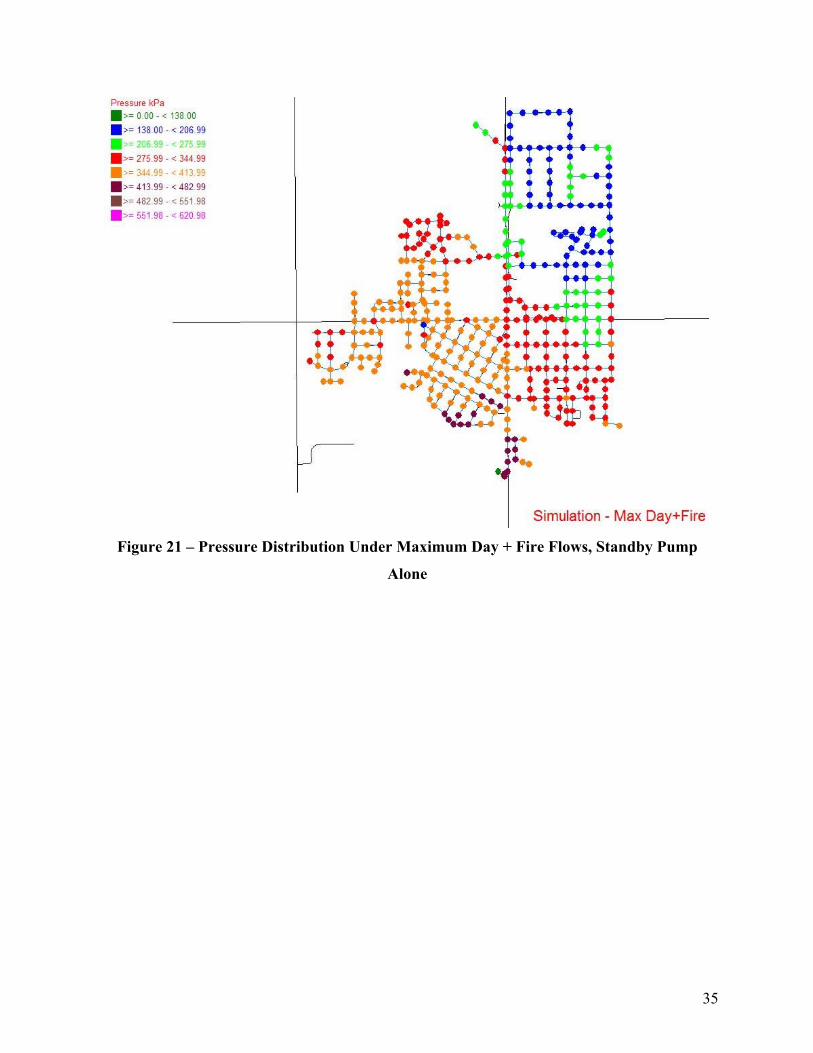
Figure 21 depicts the pressure distribution across the network during a simulation using

maximum daily flow coupled with a fire flow. As shown, the pressures are above the minimum

allowable value of 140 kPa. Thus, if the backup pump can sustain adequate pressures during an

emergency scenario, it can surely supply enough flow for other less critical conditions.

Minimum hour Average day Maximum

day

Maximum

hour

Maximum day +

fire

Flow

(L/min) 3734 3744 3767 3828 3914

Head (m) 47.2 47.1 46.8 46.1 45.2

Efficiency

(%) 84.7 84.8 84.9 85.1 85.3

Power (kW) 33.9 34 34.1 34.2 34.5

35

Figure 21 – Pressure Distribution Under Maximum Day + Fire Flows, Standby Pump

Alone

36

8.0 Conclusion In conclusion, the hydraulic simulations of our proposed water distribution network confirm that

our design provides an economical and robust distribution solution for the town of Barrhead.

This project is designed for a lifetime of 20 years since the pipes are anticipated to experience

some form of failure after 20 years, and therefore we recommend the town to allocate a cost for a

system inspection after 20 years of installation.

Barrhead is located in Alberta, which is predicted to experience a transition from an oil and gas

economy to renewable energy, which will most likely increase the town’s population. Barrhead

is the biggest town for the county of Barrhead, therefore we have accommodated for an

exponential increase in population. The projected consumption was calculated based on the

estimated consumption in 20 years for the given population, which includes future housing

development projects. The maximum daily, peak hourly, minimum hourly flows, and a critical

fire situation were calculated based on this projected average consumption. The system is

designed to operate under all of these scenarios, including an emergency fire situation. The

proposed water distribution network is optimized for the average daily flow, since this is the

scenario that will occur most commonly.

The hydraulic simulations indicated the need to tradeoff between providing adequate water

pressures or allowing for adequate velocities. Making sure that the water pressure is within the

accepted ranges is prioritized in order to ensure that all locations in the water distribution

network will receive adequate water. Optimizing for water pressure to reduce head losses will

result in reduced operating cost and reduce risk of failure, which provides a more economic and

robust design option. In order to mitigate especially low velocities in critical locations, we

suggest installing a flushing mechanism. This will prevent water from remaining stagnant, and

will ensure that every location along the water distribution network will receive adequate flows

to meet their demand.

The pumps will have to be replaced every 5 years in order to provide safe and adequate water

distribution. One item that is worth looking into is modulating the operations of the parallel

pumps. Having them continuously operated consumes a lot of energy and could decrease the

37

lifespan of the equipment. An easy solution would be to add variable frequency drives, which

will yield interesting energy savings without compromising the efficiency of the system.

Other aspects to consider would be the social acceptance of the project in the community of

Barrhead, and further research would be required to investigate the potential ecological damage

inflicted to Paddle River from the water pumping operations.

38

References ACIS. 2016. Current and Historical Alberta Weather Station Data Viewer. Alberta. Available

from: http://agriculture.alberta.ca/acis/alberta-weather-data-viewer.jsp

Alberta Community Profiles. 2016. County of Brarhead No. 11. Available from:

http://albertacommunityprofiles.com/Profile/Barrhead_No_11_County_of/255

Briere, F. C. 1999. Drinking water, distribution, sewage, and rainfall collection. Polytechnique

International Press.

CGI Group Inc. 1999. Fire Underwriters Survey: Water Supply for Public Fire Protection.

CityData. 2016. Barrhead – Town, Alberta, Canada. Available from: http://www.city-

data.com/canada/Barrhead-Town.html

DOW. 2008. Tech Solutions 605.0: Calculating Insulation Needs to Fight Frost Heave by

Comparing Freezing Index and Frost Depth. Available from:

http://msdssearch.dow.com/PublishedLiteratureDOWCOM/dh_01f6/0901b803801f6296.pdf?file

path=styrofoam/pdfs/noreg/178-00754.pdf&fromPage=GetDoc

Engineered Software Inc. 2016. Pump-Flo. Available at: https://eng-

software.com/products/pump-flo/

GCSAA. 2009. Golf Course Environmental Profile Volume II: Water Use and Conservation

Practices on US Golf Courses. Available from:

https://www.gcsaa.org/Uploadedfiles/Environment/Environmental-Profile/Water/Golf-Course-

Environmental-Profile--Water-Use-and-Conservation-Report.pdf

Georg Fischer Harvel LLC. 2016. Dimensions - Schedule 40 & 80 Pipe - PVC Industrial &

Industrial PLUS. Available from:

http://www.harvel.com/piping-systems/harvel-pvc-pipe/schedule-40-80/dimensions

39

Gov. of Alberta. 2016. Alberta Water Wells. Available from:

http://groundwater.alberta.ca/WaterWells/d/

Gov. of Alberta. 2016. Flood Hazard Identification Program. Barrhead – Paddle River – Flood

Hazard Study – Summary. Available from: http://aep.alberta.ca/water/programs-and-

services/flood-hazard-identification-program/flood-hazard-studies/documents/Barrhead-

Paddle.pdf

Groundspeak Inc. 2016. Paddle River Dam – Rochfort Bridge, Alberta. Available from:

http://www.waymarking.com/waymarks/WMH1N0_Paddle_River_Dam_Rochfort_Bridge_Albe

rta

Hydrogeological Consultants Ltd. 1998. County of Barrhead No. 11, Parts of the Pembina and

Athabasca River Basins, Groundwater Potential Evaluation. Agriculture and Agri-Food Canada.

Integrated Publishing Inc. 2016. Centrifugal Pumps. Available from:

http://nuclearpowertraining.tpub.com/h1012v3/css/h1012v3_76.htm

ITT Industries Inc. 2005. Parallel Pumps Can Provide Multiple Benefits. Available from:

http://wea-inc.com/pdf/parrallel.pdf

Lazzrino, D. 2016. Oilsands workers call on Alberta government to retrain electricians as solar

installation specialists. Edmonton Sun. Available from:

http://www.edmontonsun.com/2016/03/21/oilsands-workers-call-on-alberta-government-to-

retrain-electricians-as-solar-installation-specialists

Shammas, N. and L. Wang. 2011. Water and Wastewater Engineering: Wastewater Supply and

Wastewater Removal. 3rd Edition. Hoboken, NJ: Wiley.

40

Statistics Canada. 2012. Population and dwelling counts, for Canada, provinces and territories,

and census subdivisions (municipalities), 2011 and 2006 censuses (Alberta). Available from:

http://www12.statcan.gc.ca/census-recensement/2011/dp-pd/hlt-fst/pd-pl/Table-

Tableau.cfm?LANG=Eng&T=302&SR=1&S=51&O=A&RPP=9999&PR=48&CMA=0

The Atlas of Canada – Toporama. Available from:

http://atlas.nrcan.gc.ca/toporama/en/index.html

Town of Barrhead. 2016. Proposed New Regional Aquatic Centre. Available from:

http://www.barrhead.ca/proposed-aquatic-centre

Town of Barrhead. 2016. Town of Barrhead. Available from: http://www.barrhead.ca

41

Appendix A – Climate Data

Figure 22 – Barrhead Climate Data (ACIS, 2016)

42

Appendix B – Population Forecasting Calculations

Geometric Growth Method: growth rate and current/future population

𝐾M = 𝑙𝑛(𝑃2011/𝑃2006)(2011 − 2006) =

𝑙𝑛(4432/4209)5 = 0.010325

𝑝𝑒𝑟𝑠𝑜𝑛𝑠𝑦𝑒𝑎𝑟

𝑃2016 = 𝑃2011 ∗ 𝑒R.RSRITU∗ TRSVWTRSS = 4432 ∗ 𝑒(R.RSRITU∗U) = 4618𝑝𝑒𝑟𝑠𝑜𝑛𝑠

𝑃2036 = 𝑃2016 ∗ 𝑒R.RSRITU∗(TRIVWTRSV) = 4618 + 𝑒(R.RSRITU∗IR) = 6295𝑝𝑒𝑟𝑠𝑜𝑛𝑠

43

Appendix C – Barrhead County Information Map

Figure 23 – Barrhead County Information Map (Town of Barrhead, 2016)

44

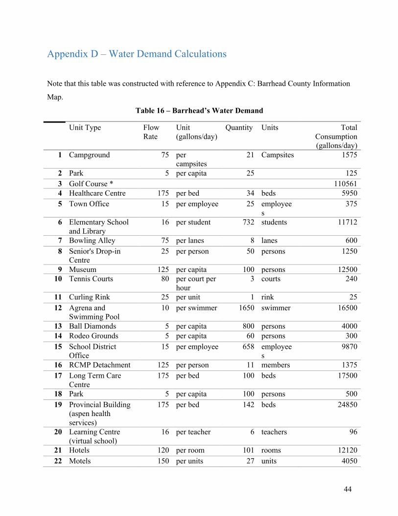
Appendix D – Water Demand Calculations

Note that this table was constructed with reference to Appendix C: Barrhead County Information

Map.

Table 16 – Barrhead’s Water Demand

Unit Type Flow Rate

Unit (gallons/day)

Quantity Units Total Consumption (gallons/day)

1 Campground 75 per campsites

21 Campsites 1575

2 Park 5 per capita 25 125 3 Golf Course * 110561 4 Healthcare Centre 175 per bed 34 beds 5950 5 Town Office 15 per employee 25 employee

s 375

6 Elementary School and Library

16 per student 732 students 11712

7 Bowling Alley 75 per lanes 8 lanes 600 8 Senior's Drop-in

Centre 25 per person 50 persons 1250

9 Museum 125 per capita 100 persons 12500 10 Tennis Courts 80 per court per

hour 3 courts 240

11 Curling Rink 25 per unit 1 rink 25 12 Agrena and

Swimming Pool 10 per swimmer 1650 swimmer 16500

13 Ball Diamonds 5 per capita 800 persons 4000 14 Rodeo Grounds 5 per capita 60 persons 300 15 School District

Office 15 per employee 658 employee

s 9870

16 RCMP Detachment 125 per person 11 members 1375 17 Long Term Care

Centre 175 per bed 100 beds 17500

18 Park 5 per capita 100 persons 500 19 Provincial Building

(aspen health services)

175 per bed 142 beds 24850

20 Learning Centre (virtual school)

16 per teacher 6 teachers 96

21 Hotels 120 per room 101 rooms 12120 22 Motels 150 per units 27 units 4050

45

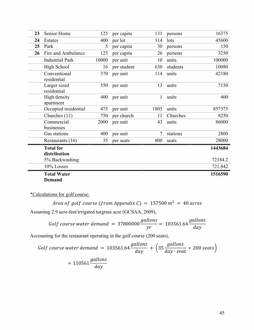
23 Senior Home 125 per capita 131 persons 16375 24 Estates 400 per lot 114 lots 45600 25 Park 5 per capita 30 persons 150 26 Fire and Ambulance 125 per capita 26 persons 3250

Industrial Park 10000 per unit 10 units 100000 High School 16 per student 630 students 10080 Conventional

residential 370 per unit 114 units 42180

Larger sized residential

550 per unit 13 units 7150

High density apartment

400 per unit 1 units 400

Occupied residential 475 per unit 1805 units 857375 Churches (11) 750 per church 11 Churches 8250 Commercial

businesses 2000 per unit 43 units 86000

Gas stations 400 per unit 7 stations 2800 Restaurants (16) 35 per seats 800 seats 28000 Total for

distribution 1443684

5% Backwashing 72184.2 10% Losses 721.842 Total Water

Demand 1516590

*Calculations for golf course:

𝐴𝑟𝑒𝑎𝑜𝑓𝑔𝑜𝑙𝑓𝑐𝑜𝑢𝑟𝑠𝑒(𝑓𝑟𝑜𝑚𝐴𝑝𝑝𝑒𝑛𝑑𝑖𝑥𝐶) = 157500𝑚T = 40𝑎𝑐𝑟𝑒𝑠

Assuming 2.9 acre-feet/irrigated turgrass acre (GCSAA, 2009),

𝐺𝑜𝑙𝑓𝑐𝑜𝑢𝑟𝑠𝑒𝑤𝑎𝑡𝑒𝑟𝑑𝑒𝑚𝑎𝑛𝑑 = 37800000𝑔𝑎𝑙𝑙𝑜𝑛𝑠𝑦𝑟 = 103561.64

𝑔𝑎𝑙𝑙𝑜𝑛𝑠𝑑𝑎𝑦

Accounting for the restaurant operating in the golf course (200 seats),

𝐺𝑜𝑙𝑓𝑐𝑜𝑢𝑟𝑠𝑒𝑤𝑎𝑡𝑒𝑟𝑑𝑒𝑚𝑎𝑛𝑑 = 103561.64𝑔𝑎𝑙𝑙𝑜𝑛𝑠𝑑𝑎𝑦 + 35

𝑔𝑎𝑙𝑙𝑜𝑛𝑠𝑑𝑎𝑦 ∙ 𝑠𝑒𝑎𝑡 ∗ 200𝑠𝑒𝑎𝑡𝑠

= 110561𝑔𝑎𝑙𝑙𝑜𝑛𝑠𝑑𝑎𝑦

46

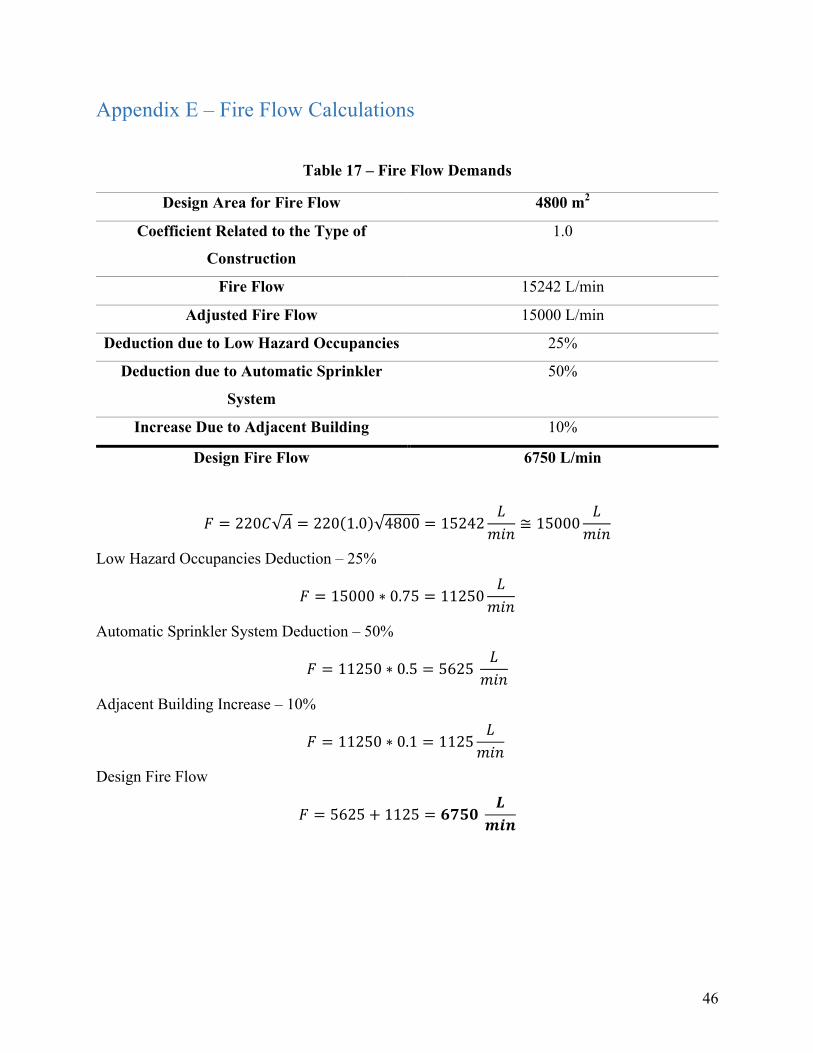
Appendix E – Fire Flow Calculations

Table 17 – Fire Flow Demands

Design Area for Fire Flow 4800 m2

Coefficient Related to the Type of

Construction

1.0

Fire Flow 15242 L/min

Adjusted Fire Flow 15000 L/min

Deduction due to Low Hazard Occupancies 25%

Deduction due to Automatic Sprinkler

System

50%

Increase Due to Adjacent Building 10%

Design Fire Flow 6750 L/min

𝐹 = 220𝐶 𝐴 = 220 1.0 4800 = 15242𝐿𝑚𝑖𝑛 ≅ 15000

𝐿𝑚𝑖𝑛

Low Hazard Occupancies Deduction – 25%

𝐹 = 15000 ∗ 0.75 = 11250𝐿𝑚𝑖𝑛

Automatic Sprinkler System Deduction – 50%

𝐹 = 11250 ∗ 0.5 = 5625𝐿𝑚𝑖𝑛

Adjacent Building Increase – 10%

𝐹 = 11250 ∗ 0.1 = 1125𝐿𝑚𝑖𝑛

Design Fire Flow

𝐹 = 5625 + 1125 = 𝟔𝟕𝟓𝟎𝑳

𝒎𝒊𝒏

47

Appendix F – Capacities of Component Structures Calculations

𝑀𝑎𝑥𝑖𝑚𝑢𝑚𝑑𝑎𝑖𝑙𝑦𝑓𝑙𝑜𝑤 = 8,579𝑚I

𝑑𝑎𝑦

𝑀𝑎𝑥𝑖𝑚𝑢𝑚ℎ𝑜𝑢𝑟𝑙𝑦𝑓𝑙𝑜𝑤 = 12,679𝑚I

𝑑𝑎𝑦

𝐹𝑖𝑟𝑒𝑓𝑙𝑜𝑤 = 6,750𝐿𝑚𝑖𝑛 0.001

𝑚I

𝐿 1,440𝑚𝑖𝑛𝑑𝑎𝑦 = 9,720

𝑚I

𝑑𝑎𝑦

Storage Calculations

Equalizing Storage:

The simulations of hourly fluctuations were based on problem 3 in the CIVE 421 Assignment 3.

Thus, the hourly consumption rates for Barrhead were obtained by assuming the same

consumption patterns but summing it up to the maximum daily flow of 8,579 m3/day. The

obtained hourly consumption rates for the town of Barrhead is summarized in Table 18.

Table 18 – Hourly Consumption Rates on Peak Day Demand

Time Water

Consumption

(m3/h)

Time Water

Consumption

(m3/h)

12:00:00 AM 0 1:00:00 PM 463.89

1:00:00 AM 178.42 2:00:00 PM 374.68

2:00:00 AM 160.58 3:00:00 PM 374.68

3:00:00 AM 160.58 4:00:00 PM 356.84

4:00:00 AM 178.42 5:00:00 PM 392.52

5:00:00 AM 231.95 6:00:00 PM 428.21

6:00:00 AM 267.63 7:00:00 PM 517.42

7:00:00 AM 371.71 8:00:00 PM 463.89

8:00:00 AM 481.73 9:00:00 PM 446.049

9:00:00 AM 570.94 10:00:00 PM 321.15

48

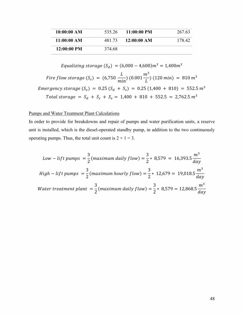
10:00:00 AM 535.26 11:00:00 PM 267.63

11:00:00 AM 481.73 12:00:00 AM 178.42

12:00:00 PM 374.68

𝐸𝑞𝑢𝑎𝑙𝑖𝑧𝑖𝑛𝑔𝑠𝑡𝑜𝑟𝑎𝑔𝑒(𝑆l) = 6,000 − 4,600 𝑚I = 1,400𝑚I

𝐹𝑖𝑟𝑒𝑓𝑙𝑜𝑤𝑠𝑡𝑜𝑟𝑎𝑔𝑒(𝑆m) = (6,750𝐿𝑚𝑖𝑛)(0.001

𝑚I

𝐿 )(120𝑚𝑖𝑛) = 810𝑚I

𝐸𝑚𝑒𝑟𝑔𝑒𝑛𝑐𝑦𝑠𝑡𝑜𝑟𝑎𝑔𝑒(𝑆n) = 0.25(𝑆l +𝑆m) = 0.25(1,400 + 810) = 552.5𝑚I

𝑇𝑜𝑡𝑎𝑙𝑠𝑡𝑜𝑟𝑎𝑔𝑒 = 𝑆l +𝑆m +𝑆n = 1,400 + 810 + 552.5 = 2,762.5𝑚I

Pumps and Water Treatment Plant Calculations

In order to provide for breakdowns and repair of pumps and water purification units, a reserve

unit is installed, which is the diesel-operated standby pump, in addition to the two continuously

operating pumps. Thus, the total unit count is 2 + 1 = 3.

𝐿𝑜𝑤 − 𝑙𝑖𝑓𝑡𝑝𝑢𝑚𝑝𝑠 =32 𝑚𝑎𝑥𝑖𝑚𝑢𝑚𝑑𝑎𝑖𝑙𝑦𝑓𝑙𝑜𝑤 =

32 ∗ 8,579 = 16,393.5

𝑚I

𝑑𝑎𝑦

𝐻𝑖𝑔ℎ − 𝑙𝑖𝑓𝑡𝑝𝑢𝑚𝑝𝑠 =32 𝑚𝑎𝑥𝑖𝑚𝑢𝑚ℎ𝑜𝑢𝑟𝑙𝑦𝑓𝑙𝑜𝑤 =

32 ∗ 12,679 = 19,018.5

𝑚I

𝑑𝑎𝑦

𝑊𝑎𝑡𝑒𝑟𝑡𝑟𝑒𝑎𝑡𝑚𝑒𝑛𝑡𝑝𝑙𝑎𝑛𝑡 =32 𝑚𝑎𝑥𝑖𝑚𝑢𝑚𝑑𝑎𝑖𝑙𝑦𝑓𝑙𝑜𝑤 =

32 ∗ 8,579 = 12,868.5

𝑚I

𝑑𝑎𝑦

49

Appendix G – Water Levels in the Elevated Reservoir

The height of the water in the elevated reservoir on an average day:

(23 − 0.8)𝑚 = 22.2𝑚

The height of the water in the elevated reservoir during a maximum daily water use:

Taking maximum average daily flow sustained for 12 hours as the critical flow, the maximum

volume of water leaving the reservoir can be calculated.

3690.94𝐿

𝑚𝑖𝑚 ∗ 60𝑚𝑖𝑛ℎ ∗

𝑚I

1000𝐿 = 221.43𝑚I

ℎ ∗ 12ℎ = 2657.13𝑚I

Subtracting this value from the volume of the reservoir to calculate for the volume left over in

storage,

2808 − 2657.13 𝑚I = 150.87𝑚I

Calculating for the height,

𝑉 =𝜋𝑑Tℎ4

ℎ =4𝑉𝜋𝑑T =

4 150.87𝑚𝜋(5𝑚T) = 7.68𝑚

50

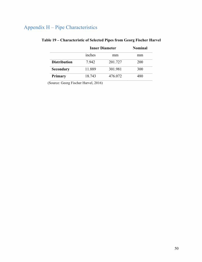
Appendix H – Pipe Characteristics

Table 19 – Characteristic of Selected Pipes from Georg Fischer Harvel

Inner Diameter Nominal

inches mm mm

Distribution 7.942 201.727 200

Secondary 11.889 301.981 300

Primary 18.743 476.072 480

(Source: Georg Fischer Harvel, 2016)