City shapes that maximize the number of walking-only trips

Bulletin of the JSME

Journal of Advanced Mechanical Design, Systems, and ManufacturingVol.14, No.5, 2020

© 2020 The Japan Society of Mechanical Engineers[DOI: 10.1299/jamdsm.2020jamdsm0075]Paper No.19-00637

City shapes that maximize the number of walking-only tripsbased on Manhattan distance

Shiori MISAKI∗ and Ken-ichi TANAKA∗∗∗Graduate School of Science and Technology, Keio University

3-14-1 Hiyoshi, Kohoku-ku, Yokohama, Kanagawa, 223-8522, Japan∗∗ Faculty of Science and Technology, Keio University

3-14-1 Hiyoshi, Kohoku-ku, Yokohama, Kanagawa, 223-8522, JapanE-mail: [email protected]

AbstractVarious modes of transportation are available when people travel within cities, and trips can be classified into twotypes depending on whether some type of vehicle is used. Compared to vehicular travel, trips conducted onlyby walking have the advantages of lower environmental impact and less space required for road networks. Byassuming that the proportion of walking-only trips decreases exponentially with the distance traveled, we explorethe problem of finding a city shape with a fixed land area that maximizes the number of walking-only trips based onManhattan distance. For many-to-one travel with the city center as the destination, we show that the optimal cityshape is a diamond. For many-to-many travel, a method is presented that expresses the number of walking-onlytrips as a double integral, originally formulated as a four-dimensional integral. Using this, an optimization problemis formulated whose variables are the vertex coordinates of a polygon, and approximate solutions for the optimalcity shape under several different settings are obtained numerically. For many-to-many travel, it is shown that alarge number of walking-only trips occur when the city shape is close to being circular, although the exact shapevaries with the distance deterrence coefficient.

Keywords : Optimal city shape, Walking-only trips, Walking probability, Manhattan distance

1. Introduction

When people travel within a city, they often have the choice of various modes of transportation, such as walking,bicycles, vehicles, and trains. Broadly speaking, such trips can be divided into those that can be conducted only bywalking and those that involve some type of vehicle. Of the two types of trips, walking trips have the advantages ofbeing environmentally friendly and requiring relatively little space for road networks. Therefore, it is important to buildmathematical models for estimating the number of walking trips in a city area. Furthermore, an important research topicto explore is the ideal shape of a city in which many trips are conducted by walking only. The purpose of this paper is toaddress this problem mathematically and obtain basic knowledge about optimal city shapes.

In general, a walking trip that uses no type of vehicle from origin to destination occurs when the travel distancebetween origin and destination is short enough. Hereinafter, we refer to this type of trip as a walking-only trip. However, asthe travel distance increases, people tend to use other modes of transportation such as bicycles, cars, and trains. To describethis trend, we assume that the percentage of people who choose a walking-only trip decreases exponentially with the triplength. Under this assumption, we construct city models that have a rectangular grid network, and we explore the cityshape that maximizes the number of walking-only trips when the travel distance is given by the Manhattan distance. TheManhattan distance has been extensively used in describing distances in urban road networks. It is frequently employedin developing mathematical models for transpotation and locational analysis (Averbakh et al. 2015; Bender et al. 2008;Larson and Odoni 1981; Vaughan 1987). Especially, there are existing literature assuming the Manhattan distance thatdeals with optimal city shapes to minimize the total travel distance (e.g., Bender et al. 2008; Demaine et al. 2011). Thus,

Received: 9 December 2019; Revised: 20 March 2020; Accepted: 11 May 2020

1

2© 2020 The Japan Society of Mechanical Engineers[DOI: 10.1299/jamdsm.2020jamdsm0075]

Misaki and Tanaka, Journal of Advanced Mechanical Design, Systems, and Manufacturing, Vol.14, No.5 (2020)

it is valuable to construct mathematical models to explore the basic characteristic of the Manhattan distance by focusingon the number of walking-only trips within a city.

Various previous studies have evaluated the basic characteristics of road network patterns using simple city shapessuch as circular or rectangular. Such studies often assume infinitely dense networks to allow analytical approaches andto derive concrete results. The expected distances and their distribution are well-studied research topics by assuming thattrip origins and destinations are uniformly and independently distributed over the city area. This continuous descriptionof urban areas is known as the continuous approximation approach. See for example Vaughan (1987) and Larson andOdoni (1981) for various continuous approximation models regarding urban analysis and transportation problems. Con-tinuous approximation models often employ a geometrical probability approach (Mathai, 1999; Solomon, 1978). Forexample, the average Euclidean distances and their distributions have been calculated for various city shapes based onuniformly and independently distributed origins and destinations. The purpose of the continuous approximation approachis to use a boldly simplified model and obtain explicit results analytically. Using the continuous approximation approach,we explore how the city shape that maximizes the number of walking-only trips with a grid network changes dependingon several input parameters.

Rather than specifying the city shape, some previous studies have sought the optimum shape. For example, Karp etal. (1975) considered the shapes of two-dimensional regions with a fixed land area in which many trips could be conductedefficiently. They obtained city shapes that minimized the average Manhattan distance and the average maximum distancebetween any two points uniformly and independently chosen within a city. They also showed that there is an approximatesolution method for finding an optimal shape to a desired level of accuracy by solving a differential equation. The optimalshape obtained by their method was shown to be close to a circle for both the Manhattan distance and the maximumdistance. Bender et al. (2004) proposed a similar problem focusing on the Manhattan distance, and they presented cityshapes based on the variational method. Their method has been further extended so that it can be used to calculate optimalshapes based on a general Lp metric (Bender et al. 2007). These are treated as problems in continuous space, but somestudies have discussed similar problems in a discrete framework (Avin et al. 2015; Bender et al. 2008; Demaine et al.2011; Fekete et al. 2014). Other studies have sought to minimize the average time required for the optimal form ofthree-dimensional cities and buildings assuming vertical movement (Johnson 1992; Suzuki 1993; Koshizuka 1995).

However, none of the aforementioned studies was focused explicitly on the mode of transportation used when travel-ing except that some studies set different speed for vertial and horizontal movement (e.g, Koshizuka 1995). The viewpointof maximizing the number of walking-only trips in a city based on the walking probability is a new approach that canprovide new insights into optimal city shapes. Herein, we use the approach of Bender et al. (2004) for the problem ofmaximizing the number of walking-only trips in a city of arbitrary shape. In addition to the problem of finding the optimalshape of an urban area, the proposed method has applications in various other situations. For example, building a newbridge in an area divided by a river will shorten some trips, and some people will switch from using a vehicle to walking.In doing so, important urban engineering issues must be addressed, such as how the number of walking trips changesdepending on the bridge position and where is the optimal bridge position that maximizes the number of walking-onlytrips. The proposed framework may also be applied to estimating the required number of moving vehicles in large areassuch as factories, theme parks, and event venues, and to designing areas with few such vehicles.

This paper is organized as follows. In Section 2, we describe city models with a grid-type network and introducethe walking probability function. In addition, by using person-trip survey data, we show that the walking probability ineach distance range fits well with the proposed exponential deterrence model. In Section 3, we deal with the city modelbased on the many-to-one trip pattern. Given a city with a fixed area and assuming that all trips are to the center andoriginate from uniformly distributed points, we show that the city shape that maximizes the number of walking-only tripsis a diamond regardless of the distance deterrence coefficient. In Sections 4–6, we deal with models that assume themany-to-many trip pattern. First, in Section 4, we derive the number of walking-only trips in the urban shapes often usedin previous studies (i.e., a circle, a square, and a diamond), and we compare the results. In Section 5, we show howto derive the number of walking-only trips for an arbitrary city shape. The total number of walking trips is expressedoriginally as a four-dimensional integral with respect to the two-dimensional coordinates of the origin and destination,but such a formulation is difficult to treat even numerically. We therefore present a method for reducing this integral to atwo-dimensional integral that is much easier to treat. In Section 6, we analyze the numerically obtained solutions in detailfor the problem of maximizing the number of walking-only trips, assuming a general city shape. Finally, in Section 7 wesummarize the present research and discuss future issues.

2



2. Basic assumptions and model description2.1. City model

In this section, we explain the basic assumptions and describe the proposed model. Our approach and notation arebased on those of Bender et al. (2004). As shown in Fig. 1, we consider a planar convex region D of arbitrary shape witharea S and that has an infinitely dense rectangular grid network. The city boundary in the first quadrant (x ≥ 0, y ≥ 0) ofthis region is denoted by w(x) (0 ≤ x ≤ a), and let (b, b) be the intersection of w(x) and y = x. We assume the followingabout the city:

(i) the city shape is symmetric with respect to the x and y axes and y = x and y = −x, and denote by h(x) and g(x) theparts 0 ≤ x ≤ b and b ≤ x ≤ a, respectively, in the first quadrant;

(ii) the boundary function w(x) is a strictly monotonic decreasing function with respect to x;

(iii) the region boundaries h(x) and g(x) are differentiable in the ranges 0 < x < b and b < x < a, respectively.

Fig. 1 Arbitrarily shaped city model with rectangular grid network.

Assumptions (i) and (ii) mean that h(x) and g(x) are mutually inverse:

h(x) = g−1(x). (1)

Furthermore, because of the symmetry, the total area of the city is eight times that of the y ≥ x part of the first quadrant:

S = 8∫ b

0{h(x) − x} dx. (2)

2.2. Walking probabilityUsually, various transportation modes are available for traveling between two locations in a city. For short journeys,

people tend to walk, whereas they tend to use vehicles such as bicycles and cars for longer journeys. Therefore, ingeneral, the probability of a person selecting a walking-only trip among several alternative modes of transportation canbe expressed as a decreasing function of the travel distance. Herein, we use an exponential function to describe thisdecreasing trend. More concretely, we denote the probability p as a function of the travel distance r as

p(r) = exp(−λr), (r ≥ 0). (3)

In the following, we refer to this function as the walking probability. As shown in Fig. 2, when the travel distance is smallenough, almost all trips are walking trips, and the probability of choosing a walking-only trip decreases exponentiallywith the travel distance. The degree of decrease is determined by λ: when λ is large, people dislike walking far and tendto select a vehicle as the mode of transportation, whereas small λ allows many people to walk a long distance.

In a previous study, Tirachini (2015) focused on walking as a mode of transportation when traveling in a city, andanalyzed the trip-length distributions of walking based on the results of origin–destination surveys conducted in severalcities around the world. Tirachini showed that the exponential distribution

f (r) = λ exp(−λr), (r ≥ 0) (4)

3



1

probabiliy of using vehicle

probabiliy of walking

Fig. 2 Walking probability p(r) as a function of travel distance r.

well-approximates the actual data of trips which are conducted by walking only. Using the exponential distribution, hecompared the estimated values of λ for various cities. In Eq. (4), 1/λ represents the expected value of the walking distance.

The above result by Tirachini (2015) is pertinent to the present study in that the former shows that more people walkwhen the travel distance is small. However, note that Eqs. (3) and (4) have different meanings. The walking probabilityp(r), which is the present focus, represents the ratio of people with travel distance r who choose to walk all the way fromorigin to destination. In this paper, we assume that the walking probability depends only on the travel distance.

Before formulating the number of walking-only trips, it is worthwhile examining how the proposed model functionp(r) describes the trend of the rate of walking-only trips in each distance range using actual travel data. Here, we usethe results of the 2015 nationwide person-trip survey (Ministry of Land, Infrastructure, Transport and Tourism 2015).These include actual travel data on selection of mode of transportation in each distance range based on the results of alarge-scale questionnaire survey conducted on both weekdays and holidays. The target cities are the major metropolitanareas of Tokyo, Osaka, and Nagoya, as well as large cities in other areas. The number of households surveyed was around47,300, the questionnaire collection rate was 29.2%, and all distances were aggregated to the nearest 0.1 km. Using thedata, we can classify trips into two types, namely, (i) those in which only walking was used and (ii) those in which adifferent mode of transportation or a combination of several modes of transportation was used. By taking the ratio of thenumber of trips of type (i) to the sum of both types in each distance range, we can evaluate the actual decreasing trend ofwalking-only trips as the distance range increases.

Figure 3 shows the proportion of walking-only trips for each distance range for weekday and holiday trips in thethree metropolitan areas, Tokyo, Osaka and Nagoya (Three MAs), and large cities in other areas (Large CAs). Thelarge cities include cities with high population such as Sapporo, Sendai and Hiroshima and large local cities such asKanazawa, Hirosaki and Takasaki. For more concrete information, see the data description of the 2015 nationwide person-trip survey (URL: http://www.mlit.go.jp/common/001229430.pdf). In the figure, we also show the graphs of p(r)for which λ was estimated by applying the least-squares method to the actual data. From Fig. 3, the decreasing trendof the proportion of actual walking-only trips fits well with the model function p(r). Therefore, we use the exponentialmodel as a macroscopic description of walking-only trips.

Note that many trip-choice behavioral models have been proposed to date, such as logit models. However, animportant characteristic of the model function p(r) is that it is much simpler than other such transportation-mode choicemodels. Because of the goodness of fit and the simplicity of the model, using the walking probability p(r) is well suitedto the purpose of the present study.

3. Optimal city shape for many-to-one travel pattern

In this section, we consider the many-to-one travel pattern in which journeys originate from uniformly distributedpoints in the region and end at a fixed destination at the center. We denote a region by D that has a fixed area S , and weseek the optimal city shape that maximizes the number of walking-only trips. This problem arises, for example, whendesigning the shape of the catchment area for a central facility that minimizes the required parking space (because itminimizes the number of car drivers who access the facility). This many-to-one travel pattern also applies when designinga grid-network city that has a fixed population and a central business district. The problem can be regarded as that offinding the city shape that minimizes the number of vehicle trips. We denote the coordinates of the trip origin by (x, y)and assume the following:

4



Fig. 3 Proportion of walking-only trips in each distance range for 2015 person-trip survey and estimated p(r):(a) weekdays; (b) holidays.

Table 1 Proportion of walkers selected by distance zone (weekdays and holidays)

Weekdays Holidaysdist r Three MAs Large CA dist r Three MAs Large CAs

0.1km∼ 0.8338 0.8015 0.1km∼ 0.8371 0.82140.2km∼ 0.7743 0.6598 0.2km∼ 0.8024 0.62330.5km∼ 0.6573 0.5229 0.5km∼ 0.6028 0.43751.0km∼ 0.4555 0.3638 1.0km∼ 0.3768 0.23051.5km∼ 0.3547 0.3292 1.5km∼ 0.2117 0.13772.0km∼ 0.2062 0.1717 2.0km∼ 0.1465 0.09463.0km∼ 0.0922 0.0842 3.0km∼ 0.0797 0.05234.0km∼ 0.0449 0.0350 4.0km∼ 0.0475 0.02775.0km∼ 0.0166 0.0133 5.0km∼ 0.0224 0.0108

(i) the trip origins are distributed uniformly and continuously over region D;

(ii) a trip maker chooses a shortest path to the destination, that is, the distance from the origin (x, y) to the center is givenby the Manhattan distance |x| + |y|.

To formulate the number of walking-only trips, we introduce the origin density function µ(x, y). This gives thenumber of trips arising from a unit area (in a unit time) around (x, y), and µ(x, y) satisfies∫

(x,y)∈Dµ(x, y)dxdy = N, (5)

where N is the total number of trips within the entire region D.Herein, we focus on the most basic and important uniform case as assumed above, which gives the trip density as

µ(x, y) = µuni =NS. (6)

This uniform distribution has been used most extensively in the literature (Larson and Odoni 1981; Vaughan 1987), whichoften gives us the tractable results and important implications.

Using this, we formulate the number of walking-only trips, F[w(x)]. The walking probability from (x, y) is given bye−λ(|x|+|y|) because the Manhattan distance from the center is |x| + |y|. F[w(x)] is formulated as

F[w(x)] = µuni

[∫ a

0

∫ w(x)

−w(x)e−λ(|x|+|y|)dydx +

∫ 0

−a

∫ w(−x)

−w(−x)e−λ(|x|+|y|)dydx

]= 4µuni

∫ a

0

∫ w(x)

0e−λ(x+y)dydx. (7)

The second equation holds because by symmetry F[w(x)] is four times the number of walking-only trips whose originsare in the first quadrant. The number of walking-only trips can be rewritten as follows using g(x) and h(x):

F[h(x), g(x)] = 4µuni

[∫ b

0

∫ h(x)

0e−λ(x+y)dydx +

∫ a

b

∫ g(x)

0e−λ(x+y)dydx

]. (8)

5



Next, we exploit the symmetry about y = x as mentioned in Section 1, that is, g is the inverse of h. By denoting g(x) = γ,we obtain x = g−1(γ) = h(γ) and dx/dγ = h′(γ). Using this relationship, the number of walking-only trips is written as

F[h] = 4µuni

[∫ b

0

∫ h(x)

0e−λ(x+y)dydx +

∫ 0

b

∫ γ

0e−λ(h(γ)+y)h′(γ)dydγ

]= 4µuni

[∫ b

0

{−1λ

e−λh(x)e−λx +1λ

e−λx}

dx +∫ 0

b

{−1λ

e−λh(γ)e−λγh′(γ) +1λ

e−λh(γ)h′(γ)}

dγ]

=4µuni

λ

{−2∫ b

0e−λ(h(x)+x)dx − 1

λe−2λb +

1λ

}. (9)

Using the above notation, the problem of seeking the shape of region D that maximizes the number of walking-onlytrips from uniformly distributed points to the center for a fixed area S can be formulated as follows.

Problem 1: Optimal shape problem for many-to-one travel pattern

maximize F[h] =4µuni

λ

{−2∫ b

0e−λ(h(x)+x)dx − 1

λe−2λb +

1λ

}(10)

subject to 8∫ b

0{h(x) − x} dx = S (11)

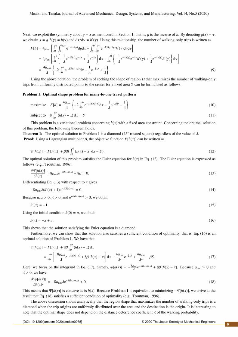
This problem is a variational problem concerning h(x) with a fixed area constraint. Concerning the optimal solutionof this problem, the following theorem holds.Theorem 1: The optimal solution to Problem 1 is a diamond (45◦ rotated square) regardless of the value of λ.Proof: Using a Lagrangian multiplier β, the objective function F[h(x)] can be written as

Ψ[h(x)] = F[h(x)] + β(8∫ b

0{h(x) − x} dx − S ). (12)

The optimal solution of this problem satisfies the Euler equation for h(x) in Eq. (12). The Euler equation is expressed asfollows (e.g., Troutman, 1996):

δΨ[h(x)]δh(x)

= 8µunie−λ(h(x)+x) + 8β = 0. (13)

Differentiating Eq. (13) with respect to x gives

−8µuniλ(h′(x) + 1)e−λ(h(x)+x) = 0. (14)

Because µuni > 0, λ > 0, and e−λ(h(x)+x) > 0, we obtain

h′(x) = −1. (15)

Using the initial condition h(0) = a, we obtain

h(x) = −x + a. (16)

This shows that the solution satisfying the Euler equation is a diamond.Furthermore, we can show that this solution also satisfies a sufficient condition of optimality, that is, Eq. (16) is an

optimal solution of Problem 1. We have that

Ψ[h(x)] = F[h(x)] + 8β∫ b

0{h(x) − x} dx

=∫ b

0

[−8µuni

λe−λ(h(x)+x) + 8β {h(x) − x}

]dx − 4µuni

λ2 e−2λb +4µuni

λ2 − βS . (17)

Here, we focus on the integrand in Eq. (17), namely, ψ[h(x)] = − 8µuniλ

e−λ(h(x)+x) + 8β {h(x) − x}. Because µuni > 0 andλ > 0, we have

∂2ψ[h(x)]∂h(x)2 = −8µuniλe−λ(h(x)+x) < 0. (18)

This means that Ψ[h(x)] is concave as is h(x). Because Problem 1 is equivalent to minimizing −Ψ[h(x)], we arrive at theresult that Eq. (16) satisfies a sufficient condition of optimality (e.g., Troutman, 1996).

The above discussion shows analytically that the region shape that maximizes the number of walking-only trips is adiamond when the trip origins are uniformly distributed over the area and the destination is the origin. It is interesting tonote that the optimal shape does not depend on the distance deterrence coefficient λ of the walking probability.

6



4. Results for cities with specific shapes

In Sections 4 and 5, we assume the many-to-many trip pattern and derive the total number of walking-only trips. Inthe present section, we focus on cities with the specific shapes shown in Fig. 4, namely, a circle, a square, and a diamond,and we calculate the number of walking-only trips. The results presented in the present section are compared in Section 5when more-general city shapes are assumed.

The average travel distances and their distribution for circles and squares have been dealt with extensively in theliterature. Mathematical models that assume travel on a continuous plane using simple city shapes are summarized indetail by Vaughan (1987). In particular, with regard to the Manhattan distance, there is accumulated research on thecircle, square, and diamond shapes as shown in Fig. 4.

In the following, we introduce the existing research that derives the distribution of the Manhattan distance assuminga uniform trip between any two points in these three city models. We then describe the method for deriving the totalnumber of walking-only trips using the distance distribution, and we present some results.

Fig. 4 City models with specific shapes: (a) circle; (b) square; (c) diamond.

In the following, we denote the origin by P(x1, y1) and the destination by Q(x2, y2), and we assume the following:

(i) the origins and destinations of trips are uniformly and independently distributed within the city;

(ii) a traveler chooses the shortest path on a rectangular grid network, and thus the Manhattan distance between P(x1, y1)and Q(x2, y2) is given by |x1 − x2| + |y1 − y2|.

We introduce the trip density ρ(x1, y1, x2, y2) to describe the total number of walking-only trips, which gives thenumber of trips originating from a small zone with area dx1dy1 at P(x1, y1) and terminating in a small zone with areadx2dy2 at Q(x2, y2) as

ρ(x1, y1, x2, y2)dx1dy1dx2dy2. (19)

The total number of trips in the city, N, is related to the trip density by∫(x1,y1)∈D

∫(x2,y2)∈D

ρ(x1, y1, x2, y2)dy2dx2dy1dx1 = N. (20)

Using the trip density, the total number of walking-only trips is given as

F[w] =∫

(x1,y1)∈D

∫(x2,y2)∈D

ρ(x1, y1, x2, y2)e−λ(|x1−x2 |+|y1−y2 |)dy2dx2dy1dx1. (21)

As noted in assumption (i), we consider the most basic and important uniform case for the trip density:

ρ(x1, y1, x2, y2) = ρuni =NS 2 . (22)

The case in which trip origins and destinations are uniformly and independently distributed is the one that is used mostoften in existing city models. In particular, a circular city is known as a Smeed city after Ruben Smeed, who contributedgreatly to the development of continuous transportation modeling (Vaughan, 1987).

Meanwhile, if the distance distribution is already known, as it is in the present section, we need only perform the one-dimensional integration described below instead of the general expression of Eq. (21). The distance distribution refers tothe probability density function of the distance traveled within a city based on the continuous trip density. In other words,for the distance distribution φ(r), the proportion of travelers whose travel distance lies in the small range [r, r + dr] is

7



given by φ(r)dr. If the distance distribution φ(r) is known for a particular city model, then N × p(r) × φ(r)dr representsthe number of trips whose travel distance is in the range [r, r + dr] and the travel is conducted by walk only. Therefore,the overall number of walking-only trips can be represented as

F = N∫ ∞

0p(r)φ(r)dr. (23)

Kurita (2001) derived the distribution of the Manhattan distance for a circular city of radius R as

φcir(r) =

4π

∫ r

r/√

2

g(u)√

2u2 − r2du (0 ≤ r ≤ 2R),

4π

∫ 2R

r/√

2

g(u)√

2u2 − r2du (2R ≤ r ≤ 2

√2R),

(24)

where g(u) is the distribution of the Euclidean distance for two points uniformly and independently distributed within acircular city (Vaughan, 1987; Mathai, 1999), namely,

g(u) =4rπR2 arccos

( r2R

)− r2

πR4

√4R2 − r2 (0 ≤ r ≤ 2R). (25)

The distance distribution for a square city with side length L is given as

φsq(r) =

1

3L4

(2r3 − 12Lr2 + 12L2r

)(0 ≤ r ≤ L),

23L4 (2L − r)3 (L ≤ r ≤ 2L),

(26)

and Tanaka et al. (2007) derived the distance distribution in a diamond city as

φdia(r) =1L4

(r3 − 3

√2Lr2 + 4L2r

)(0 ≤ r ≤

√2L). (27)

Here, by applying Eq. (23) for the number of walking-only trips within a city to the distance distributions of Eqs. (26) and(27), we obtain the total numbers of walking-only trips for the square (Fsq) and diamond (Fdia) cities as

Fsq = N{

4λ4L4

(1 + e−2λL − 2e−λL

)− 8λ3L3

(1 − e−λL

)+

4λ2L2

}, (28)

Fdia = N

6λ4L4

(1 − e−

√2λL)− 6√

2λ3L3 +

2λ2L2

(2 + e−

√2λL) . (29)

For the circular city, obtaining the total number of walking-only trips, Fcir, involves numerical integration because thedistance distribution is expressed in integral form as shown in Eq. (24).

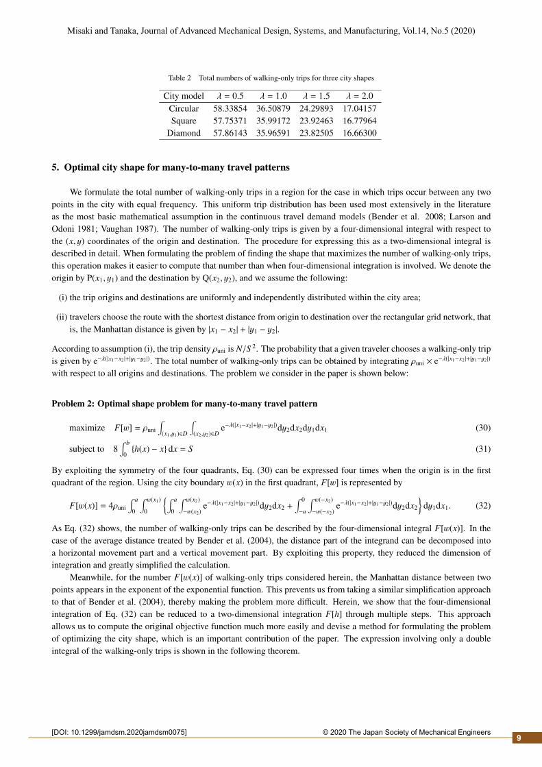
Let us compare the total numbers of walking-only trips Fcir, Fsq, and Fdia for the three different city shapes with thesame area. We set the area of each city as S = π, that is, the square and the diamond have side length

√π ≈ 1.77, and

the circle has unit radius. We set N = 100 and focus on four different distance deterrence values: λ = 0.5, 1.0, 1.5, and2.0. The results for the total numbers of walking-only trips for the three cities are summarized in Table 2, from which itcan be seen that the total number of walking-only trips decreases with λ. Of the three shapes, the circular city realizes thelargest number of walking-only trips. In Section 3, we showed that the optimal shape for many-to-one trips to the centeris a diamond, whereas Table 2 shows that the circular city performs best for all four values of λ. It is interesting that forthe many-to-many trip pattern the circular city performs better than the diamond city. Looking at the details, the diamondcity is more advantageous than the square when λ = 0.5, but the square is better than the diamond for other values ofλ. As such, the desirable city shape changes depending on the value of the distance deterrence coefficient, which is aninteresting finding of the proposed model.

The above analysis showed that the circular shape is the most advantageous of the three city shapes. A naturalquestion that arises here is whether there is a better shape than the circle. In Section 5, to answer this question, we analyzethe number of walking-only trips for more-general city shapes, assuming uniform trips between any two points in the city.

8



Table 2 Total numbers of walking-only trips for three city shapes

City model λ = 0.5 λ = 1.0 λ = 1.5 λ = 2.0Circular 58.33854 36.50879 24.29893 17.04157Square 57.75371 35.99172 23.92463 16.77964

Diamond 57.86143 35.96591 23.82505 16.66300

5. Optimal city shape for many-to-many travel patterns

We formulate the total number of walking-only trips in a region for the case in which trips occur between any twopoints in the city with equal frequency. This uniform trip distribution has been used most extensively in the literatureas the most basic mathematical assumption in the continuous travel demand models (Bender et al. 2008; Larson andOdoni 1981; Vaughan 1987). The number of walking-only trips is given by a four-dimensional integral with respect tothe (x, y) coordinates of the origin and destination. The procedure for expressing this as a two-dimensional integral isdescribed in detail. When formulating the problem of finding the shape that maximizes the number of walking-only trips,this operation makes it easier to compute that number than when four-dimensional integration is involved. We denote theorigin by P(x1, y1) and the destination by Q(x2, y2), and we assume the following:

(i) the trip origins and destinations are uniformly and independently distributed within the city area;

(ii) travelers choose the route with the shortest distance from origin to destination over the rectangular grid network, thatis, the Manhattan distance is given by |x1 − x2| + |y1 − y2|.

According to assumption (i), the trip density ρuni is N/S 2. The probability that a given traveler chooses a walking-only tripis given by e−λ(|x1−x2 |+|y1−y2 |). The total number of walking-only trips can be obtained by integrating ρuni × e−λ(|x1−x2 |+|y1−y2 |)

with respect to all origins and destinations. The problem we consider in the paper is shown below:

Problem 2: Optimal shape problem for many-to-many travel pattern

maximize F[w] = ρuni

∫(x1,y1)∈D

∫(x2,y2)∈D

e−λ(|x1−x2 |+|y1−y2 |)dy2dx2dy1dx1 (30)

subject to 8∫ b

0{h(x) − x} dx = S (31)

By exploiting the symmetry of the four quadrants, Eq. (30) can be expressed four times when the origin is in the firstquadrant of the region. Using the city boundary w(x) in the first quadrant, F[w] is represented by

F[w(x)] = 4ρuni

∫ a

0

∫ w(x1)

0

{∫ a

0

∫ w(x2)

−w(x2)e−λ(|x1−x2 |+|y1−y2 |)dy2dx2 +

∫ 0

−a

∫ w(−x2)

−w(−x2)e−λ(|x1−x2 |+|y1−y2 |)dy2dx2

}dy1dx1. (32)

As Eq. (32) shows, the number of walking-only trips can be described by the four-dimensional integral F[w(x)]. In thecase of the average distance treated by Bender et al. (2004), the distance part of the integrand can be decomposed intoa horizontal movement part and a vertical movement part. By exploiting this property, they reduced the dimension ofintegration and greatly simplified the calculation.

Meanwhile, for the number F[w(x)] of walking-only trips considered herein, the Manhattan distance between twopoints appears in the exponent of the exponential function. This prevents us from taking a similar simplification approachto that of Bender et al. (2004), thereby making the problem more difficult. Herein, we show that the four-dimensionalintegration of Eq. (32) can be reduced to a two-dimensional integration F[h] through multiple steps. This approachallows us to compute the original objective function much more easily and devise a method for formulating the problemof optimizing the city shape, which is an important contribution of the paper. The expression involving only a doubleintegral of the walking-only trips is shown in the following theorem.

9



Theorem 2: The total number of walking-only trips (32) assuming uniform and independent point pairs under theManhattan distance can be calculated by performing the following two-dimensional integration:

F[h] = 4ρuni

[4λ2

∫ b

0

∫ u

0

{e−λ(h(u)+h(v)+u−v) − e−λ(−h(u)+h(v)+u+v) − e−λ(−h(u)+h(v)+u−v)

}dvdu

+2λ2

∫ b

0

∫ b

0

{e−λ(h(u)+h(v)−u−v) + e−λ(h(u)+h(v)+u−v) + 2e−λ(h(u)+h(v)+u+v) + e−λ(h(u)+h(v)−u+v)

}dvdu

+4λ3

∫ b

0

{e−λ(h(u)+u+2b) + e−λ(h(u)−u+2b) − e−λ(h(u)−u) − e−λ(h(u)+u)

}du

+8λ2

∫ b

0

{1 − e−2λu

}h(u)du +

1λ4

{e−4λb − 2e−2λb + 1

}+

4bλ3

{1 − e−2λb

}− 4b2

λ2

]. (33)

In the following, we show how to obtain this result according to the following five steps.

Step 1 Express all different expressions of the integrand in Eq. (32) without using absolute-value functions based on themagnitudes of the x and y coordinates.

Step 2 Delete the inverse function w−1 appearing in the integration range by variable transformation.

Step 3 Express F using g(x) and h(x) in Fig. 1 instead of w(x).

Step 4 Express F using only h(x) based on the relationship that g(x) is the inverse of h(x).

Step 5 Delete h′(x) by carrying out the integration of the composite function, and express F as a function of h only.

In the following, the total number of walking-only trips is calculated from Eq. (32) to arrive at Eq. (33) by executing theabove steps.

5.1. Step 1We denote the i-th quadrant by Ri (i = 1, 2, 3, 4) and begin with the case in which both the x and y coordinates of

origin are non-negative (i.e., the origin is in the first quadrant R1). We denote the number of walking-only trips as Fi[w](i = 1, 2, 3, 4) when the destination is in Ri (i = 1, 2, 3, 4) as shown in Fig. 5. Note that 0 < x < b and b < x < a parts ofw(x) are denoted by g(x) and h(x) respectively, as introduced in Fig. 1. Using the same argument when the origin is in aquadrant other than R1, the following relation holds:

F[w] = 4 {F1[w] + F2[w] + F3[w] + F4[w]} . (34)

Concretely, Fi[w] (i = 1, 2, 3, 4) can be expressed as Eqs. (35)–(38).

When P(x1, y1) ∈ R1 and Q(x2, y2) ∈ R1, we have

F1[w] = ρuni

{∫ a

0

∫ w(x1)

0

∫ x1

0

∫ y1

0e−λ(x1−x2+y1−y2)dy2dx2dy1dx1 +

∫ a

0

∫ w(x1)

0

∫ w−1(y1)

x1

∫ y1

0e−λ(x2−x1+y1−y2)dy2dx2dy1dx1

+∫ a

0

∫ w(x1)

0

∫ a

w−1(y1)

∫ w(x2)

0e−λ(x2−x1+y1−y2)dy2dx2dy1dx1 +

∫ a

0

∫ w(x1)

0

∫ x1

0

∫ w(x2)

y1e−λ(x1−x2+y2−y1)dy2dx2dy1dx1

+∫ a

0

∫ w(x1)

0

∫ w−1(y1)

x1

∫ w(x2)


}. (35)


F2[w] = ρuni

{∫ a

0

∫ w(x1)

0

∫ −w−1(y1)

−a

∫ w(−x2)


+∫ a

0

∫ w(x1)

0

∫ 0

−w−1(y1)

∫ y1


+∫ a

0

∫ w(x1)

0

∫ 0

−w−1(y1)

∫ w(−x2)


}. (36)

10




F3[w] = ρuni

∫ a

0

∫ w(x1)

0

∫ 0

−a

∫ 0

−w(−x2)e−λ(x1−x2+y1−y2)dy2dx2dy1dx1. (37)


F4[w] = ρuni

{∫ a

0

∫ w(x1)

0

∫ x1

0

∫ 0

−w(x2)e−λ(x1−x2+y1−y2)dy2dx2dy1dx1

+∫ a

0

∫ w(x1)

0

∫ a

x1

∫ 0

−w(x2)e−λ(x2−x1+y1−y2)dy2dx2dy1dx1

}. (38)

Fig. 5 Four cases based on destination location when origin is in R1.

11



5.2. Step 2In Eqs. (35)–(38), t = w−1(y1) leads to y1 = w(t) and dy1/dt = w′(t). Using these relations to organize these

expressions, the objective function F[w] is expressed as

F[w, w′] = 4ρuni

[1λ2

∫ a

0

∫ a

x1

{−e−λ(w(t)−x1+a) − e−λ(w(t)+x1+a) + e−λ(w(t)+x1) + e−λw(t)

+2e−λ(t−x1) + e−λ(t+x1) − e−λx1 − 2}w′(t)dtdx1

+1λ2

∫ a

0

∫ x1

0

{2e−λ(w(x1)+w(z)+x1−z) − e−λ(−w(x1)+w(z)+x1−z) − e−λ(w(x1)+x1−z)

−e−λ(w(z)+x1−z) + e−λ(x1−z) + 2λw(x1)e−λ(x1−z)}

dzdx1

+1λ2

∫ a

0

∫ a

0

{e−λ(w(x1)+w(z)+x1+z) − e−λ(w(z)+x1+z) − e−λ(w(x1)+x1+z) + e−λ(x1+z)

}dzdx1

+1λ

∫ a

0

∫ a

x1

∫ a

t

{−e−λ(w(t)−w(z)−x1+z) − e−λ(w(t)−w(z)+x1+z)

}w′(t)dzdtdx1

+1λ

∫ a

0

∫ a

x1

∫ t

x1e−λ(−w(t)+w(z)−x1+z)w′(t)dzdtdx1

+1λ

∫ a

0

∫ a

x1

∫ t

0

{e−λ(−w(t)+w(z)+x1+z) − e−λ(x1+z)

}w′(t)dzdtdx1

]. (39)

For convenience of explanation, we denote the six integral terms inside the parentheses in Eq. (39) by FA[w], FB[w],FC[w], FD[w], FE[w], and FF[w], then Eq. (39) can be expressed as

F[w] = 4ρuni {FA[w] + FB[w] + FC[w] + FD[w] + FE[w] + FF[w]} . (40)

In Step 3, F[w] represented by w(x) defined in the entire first quadrant is expressed as a functional of g(x) and h(x). Spacelimitations mean that this method is described for FA[w] only, but FB[w] through FF[w] can be obtained by the sameprocedure.

5.3. Step 3Based on the above, F[w] can be expressed using g and h. The boundary function w can be described as h for the

integral variable t in [0, b], and g in [b, a]. The same is true for the integral variable x1. By carrying out the above process,we obtain

FA[g, g′, h, h′] =1λ2

∫ b

0

∫ b

x1

{−e−λ(h(t)−x1+a) − e−λ(h(t)+x1+a) + e−λ(h(t)+x1) + e−λh(t) + 2e−λ(t−x1) + e−λ(t+x1) − e−λx1 − 2

}h′(t)dtdx1

+1λ2

∫ a

b

∫ a

x1

{−e−λ(g(t)−x1+a) − e−λ(g(t)+x1+a) + e−λ(g(t)+x1) + e−λg(t) + 2e−λ(t−x1) + e−λ(t+x1) − e−λx1 − 2

}g′(t)dtdx1

+1λ2

∫ b

0

∫ a

b

{−e−λ(g(t)−x1+a) − e−λ(g(t)+x1+a) + e−λ(g(t)+x1) + e−λg(t) + 2e−λ(t−x1) + e−λ(t+x1) − e−λx1 − 2

}g′(t)dtdx1. (41)

5.4. Step 4F[g, h, g′, h′] is expressed as a functional with only h. We show how to conduct this process by focusing on

FA[g, h, g′, h′] in Eq. (41). Due to the symmetry about y = x in the first quadrant, if we express g(x1) by γ, then therelations x1 = g−1(γ) = h(γ) and dx1/dγ = h′(γ) hold. Similarly, expressing g(t) by α leads to t = g−1(α) = h(α) anddt/dα = h′(α), Using these relations, FA[g, h] can be expressed with only h:

FA[h, h′] =1λ2

∫ b

0

∫ b

x1

{−e−λ(h(t)−x1+a) − e−λ(h(t)+x1+a) + e−λ(h(t)+x1) + e−λh(t) + 2e−λ(t−x1) + e−λ(t+x1) − e−λx1 − 2

}h′(t)dtdx1

+1λ2

∫ b

0

∫ γ

0

{−e−λ(−h(γ)+α+a) − e−λ(h(γ)+α+a) + e−λ(h(γ)+α) + e−λα + 2e−λ(h(α)−h(γ)) + e−λ(h(α)+h(γ)) − e−λh(γ) − 2

}h′(γ)dαdγ

− 1λ2

∫ b

0

∫ b

0

{−e−λ(α−x1+a) − e−λ(α+x1+a) + e−λ(α+x1) + e−λα + 2e−λ(h(α)−x1) + e−λ(h(α)+x1) − e−λx1 − 2

}dαdx1. (42)

We can apply the same procedure for FB[g, h, g′, h′] through FF[g, h, g′, h′].

12



5.5. Step 5We show how to arrive at the final results by deleting h′(x) by carrying out the integration of the composite function.

We take Eq. (42) as an example to show the method:

FA[h] =1λ3

∫ b

0

{−e−λ(h(x1)−x1+a) + e−λ(−h(x1)+x1+a) + e−2λh(x1) + 2e−λ(h(x1)+x1) − 2e−λ(h(x1)+x1+a) + e−λh(x1)

}dx1

+1λ2

∫ b

0

{−2e−2λx1 − e−λx1 + 4

}h(x1)dx1 +

1λ4

{e−λa − e−λ(a+2b) + e−2λb − 1

}+

1λ3

{−be−2λb − be−λb

}− 2b2

λ2 . (43)

By applying a similar procedure, we can obtain the expression for the number of walking-only trips as shown in Eq. (33),thereby concluding the proof.

Originally, the number of walking-only trips within a city required a four-dimensional integral. As shown in Eq. (33),this can be reduced to a two-dimensional integral in the variables u and v, thereby allowing us to compute the objectivefunction much more easily.

Next, we confirm that the number of walking-only trips in a city of a specific shape can be computed using Eq. (33).In Section 4, we presented values for the number of walking-only trips for three city shapes using the existing distancedistributions. Here, we focus on two city shapes: circular and diamond. The boundary functions of these city models,hcir(x) and hdia(x), are given as

hcir(x) =

√Sπ− x2, (44)

hdia(x) =

√S2− x, (45)

where S is the area of the city. We can compute Fcir and Fdia by applying hcir(x) and hdia(x) to h in Eq. (33). We take thecase of S = π and λ = 1.0 as an example, and carry out numerical integration using Eq. (33) using Wolfram Mathemat-ica 11.2. We obtain the numbers of walking-only trips as 36.50879 for Fcir and 35.96591 for Fdia. These results matchexactly those obtained using the distance distributions of Eqs. (24) and (27). Note that for the square city, the boundaryfunction parallel to the y axis has no inverse, and this approach cannot be used. However, in this special case we havealready obtained the analytical result of Eq. (28), which was computed from the distance distribution.

We have already shown that unlike the case of many-to-one trips, the circular city is superior to the square anddiamond cities in terms of the number of walking-only trips. In Section 6, we use Eq. (33) to explore city shapes than areeven better that the circular one.

6. Numerical results

In this section, we address numerically the problem of maximizing the number of walking-only trips using Eq. (33)derived in Section 5. As for the boundary functions, we deal with two types: the one-parameter function treated by Benderet al. (2004) and a convex polygon.

6.1. One-parameter boundary function: h(x) =(ad − xd

) 1d

Bender et al. (2004) used the following one-parameter boundary function in search of the city shape that minimizesthe average Manhattan distance between every uniform point pair:

h(x) =(ad − xd

) 1d (0 ≤ x ≤ b). (46)

By varying the value of d, Eq. (46) describes various city shapes. Important special cases are d = 1 for the diamond, d = 2for the circle, and d = ∞ for the square, which are the cases treated in Section 5. We denote the number of walking-onlytrips by Fd[h] when the border function (46) is employed. For a fixed value of d, we can compute Fd[h] by carrying out

the numerical integral as described in Eq. (33) by applying h(x) =(ad − xd

) 1d . We show some numerical results for S = π

and N = 100. Figure 6 shows the values of Fd[h] obtained by numerical integration for various values of d in the fourcases of λ = 0.5, 1.0, 1.5, and 2.0. As each graph shows, there is a value d∗ that maximizes Fd[h].

Figure 6 shows that the larger the value of λ, the larger the value of d∗. It is interesting to note that the circle is inbetween λ = 0.5 and λ = 1.0. More concretely, when λ = 0.5, d∗ ≈ 1.95, which is almost a circle but distorted slightly

13



toward a diamond. For the other three cases, we have d∗ > 2, namely, d∗ ≈ 2.08 for λ = 1.0, d∗ ≈ 2.18 for λ = 1.5,and d∗ ≈ 2.26 for λ = 2.0. Also in these cases, the optimal shapes are very close to a circle but distorted slightly towarda square. In summary, while the value of λ has some effect on the city shape, the optimal shape remains very close to acircle. This result is similar to those given by the average-distance models of Karp et al. (1975) and Bender et al. (2004).It is interesting to note that while the many-to-one optimal shape is a diamond, the many-to-many results are close to acircle. The optimum shape for many-to-many trips depends on λ, which is an interesting finding of the present paper.

In Fig. 7, the optimal shapes for λ = 0.2 and λ = 5.0 are compared to a circle. The latter relatively large value of λwas chosen to show the difference in shape more clearly. While the shapes that are shown are not perfect circles, they areclose to being so. In summary, the results show that a circular area performs well in terms of maximizing the number ofwalking-only trips within a city.

Fig. 6 Values of Fd[h] as a function of d for λ = 0.5, 1.0, 1.5, and 2.0.

Fig. 7 Optimal shapes for λ = 0.2 and 5.0.

14



6.2. Convex polygonTo explore city shapes that are better than those that arise with the one-parameter model, we consider a boundary

given by a convex polygon. In a different model, Demaines et al. (2011) showed that the optimal shape is convex whenthe average distance is used as the objective function. There are two advantages of approximating a city with a polygon:

(i) an analytical expression for the number of walking-only trips can be obtained by integrating Eq. (33) directly;

(ii) with a sufficient number of vertices, a flexible shape can be expressed.

Advantage (i) above is due to using a simple (piecewise) linear function for (convex) polygons. The problem of seekingthe optimal city shape can be regarded as an optimization problem with the vertex coordinates of the polygon as variables.Therefore, advantage (i) above has practical merit in that it enables us to solve the problem using a general-purposenonlinear optimization solver. Equation (33) allows us to use the approach of reducing the four-dimensional integrationto a two-dimensional one. Figure 8 illustrates the situation. On the boundary function h(x), the coordinates of the verticesare given by

P0(0, a),P1(s1, t1), . . . , Pn−1(sn−1, tn−1),Pn(b, b), (47)

and n segments h1(x), h2(x), . . . , hn(x) are set between adjacent points. These segments are expressed as

h1(x) =t1 − a

s1x + a (0 ≤ x ≤ s1), (48)

h j(x) =t j − t j−1

s j − s j−1(x − s j−1) + t j−1 (s j−1 ≤ x ≤ s j), j = 2, . . . , n − 1, (49)

hn(x) =b − tn−1

b − sn−1(x − sn−1) + tn−1 (sn−1 ≤ x ≤ b). (50)

Fig. 8 City shape described by a convex polygon.

By describing the boundary line h(x) by a convex polygon, the exponential function multiplier included in the ob-jective function becomes a linear expression, thereby giving the expression for the number of walking-only trips (33).However, because there exist multiple cases at the vertex coordinates, the expression is quite complicated.

Using the above notation, the problem of maximizing the number of walking-only trips can be described as

maximize Fpoly(a, b, s1, s2, · · · , sn−1, t1, t2, · · · , tn−1) (51)

subject to 8[∫ s1

0{h1(x) − x} dx +

n−1∑i=2

∫ si

si−1{hi(x) − x} dx +

∫ b

sn−1{hn(x) − x} dx

]= S . (52)

We can obtain an explicit expression for Eq. (51) by carrying out the integral in Eq. (33). The first two terms of Eq. (33)involve double integrals, which can be conducted over the region shown in Fig. 9. We can also execute the integral inEq. (52) to express the area for the polygon model.

In the following, the process for obtaining the solution of this polygon model is explained and the results are analyzed.Although both the objective function and the constraint equation can be expressed as functions of the polygonal vertexcoordinates, because they are complex nonlinear functions, it is difficult to find a global optimal solution for this problem.

15



Fig. 9 Region of integration for polygon model with n = 4: (a) first term of Eq. (33); (b) second term of Eq. (33).

Our present approach is to use a general-purpose nonlinear solver and obtain several local optimal solutions. We used theFindMaximum function in Wolfram Mathematica 11.2. As an initial solution, we used a convex polygon with a randomerror added to each coordinate of each vertex of the regular polygon. More concretely, we obtained solutions by thefollowing procedure.

Step 1 Set the coordinates of a regular polygon in the range 0 ≤ x ≤ b as (r cos θi, r sin θi), where θi = π/2− iθ̄, θ̄ = π/(4n)for i = 1, . . . , n.

Step 2 For i = 1, . . . , n − 1, generate ϵi randomly in the range [−θ̄/2, θ̄/2].

Step 3 For i = 1, . . . , n − 1, a regular polygon is distorted using ϵi to obtain a new polygon whose vertices are (r cos(θi +

ϵi), r sin(θi + ϵi)).

Step 4 Adjust the size of the polygon to satisfy the area constraint.

Step 5 Input the resulting polygon to the solver as an initial solution of the problem.

Next, we show the results of applying the above process when the city is given as a 56-sided polygon (n = 7) withS = π and N = 100. Figure 10 shows the solutions for λ = 0.2 and 5.0. For each example, we start with 30 different initialsolutions and use the best one as the solution. A circle is also drawn for the purpose of comparison. The vertex positionsof the polygon model are indicated by small dots. From this figure, the following features can be seen:

(1) λ = 0.2 gives a circular form that is distorted slightly toward a diamond;

(2) λ = 5.0 gives a circular form that is distorted slightly toward a square;

(3) both forms are quite close to a circle.

This result is similar to the conclusion obtained with the one-parameter d model. To compare the obtained results with theprevious ones, Table 3 summarizes the results of calculating the number of walking-only trips for the diamond and circleand the d and polygon models using five different values of λ. To compare the shapes obtained with the d and polygonmodels, Fig. 11 shows the optimal solutions for λ = 0.2 and 2.0, which appear to be almost identical.

As described above, the vertices of the initial polygon are distributed on the circumference of a circle, but the obtainedresults are almost the same as the d-model solution whose vertices are away from the circumference. Judging from theseresults, the solutions obtained with both models are fairly good solutions. Nevertheless, comparing the numbers ofwalking-only trips from both models in Table 3, the result with the polygon model outperforms that with the d-model forall values of λ, although the differences are admittedly extremely small. For a polygon with a medium number of vertices,we reason that the result is more than that with the d-model because of the higher degree of freedom of the polygon model.

16



Fig. 10 Solutions for polygon model (λ = 0.2 and 5.0) and a circle.

Table 3 Comparison of solutions for various city models.

λ Diamond Circle d-model Polygon (n = 7)0.2 79.6250112 79.8943626 79.8962420 79.89624480.8 43.1476236 43.6906507 43.6907989 43.69080151.4 25.7505648 26.2423639 26.2455464 26.24558762.0 16.6630038 17.0415706 17.0469903 17.04705385.0 3.9711575 4.0553191 4.0576322 4.0576542

Fig. 11 Comparison of solutions with d-model and polygon model (λ = 0.2 and λ = 2.0).

17



7. Conclusion and future research perspectives

People traveling in a city have a choice to modes of transportation, which broadly speaking can be divided intowalking and vehicles. Trips that involve only walking have the advantages of lower environmental impact and takingup less city space compared to travel using vehicles. In general, walking-only trips are made only when trip length isshort, and the proportion of vehicular use increase with the travel distance. To describe this point, we assumed that theproportion of walking-only trips decreases exponentially with the trip length.

We assumed city models with a typical rectangular grid network, and we considered the problem of determining thecity shape that maximizes the number of walking-only trips for many-to-one and many-to-many trip patterns. In the caseof the many-to-one type where the destination is the city center, we used the variational method to show that the optimalcity shape is a diamond. For the many-to-many type, we presented a method for expressing the number of walking-onlytrips by a double integral that was formulated originally as a four-dimensional integral.

Using this method, we formulated an optimization problem with the vertex coordinates of a polygon as the variables,and we obtained numerically an approximate solution for the optimal shape. As a result, we found that while the many-to-one optimal shape is a diamond, the many-to-many results are close to a circle. In addition, although the former casedoes not depend on the value of λ, the latter case depends on the value. We have also found that values of the number ofwalking-only trips are fairly stable regarding the deviation of shape from a circle and the value of λ. This result suggeststhat as long as the city shape does not deviate greatly from the circle and is roughly convex, the number of walking trips isnot much different from the maximum value. Also even when the value of λ changes due to, for example, the progress ofaging society, desirable city shapes do not change dramatically. As we have shown in the numerical results, our proposedformulation enables us how the values of λ affects the desirable city shapes, which have not been treated in the existingaverage distance (or time) minimization approach.

Maximizing the number of walking trips is equivalent to minimizing the number of trips using a vehicle. Therefore,the proposed approach is useful in reducing the space required for parking or relieving traffic jam within a city, which areimportant issues in urban planning. Based on the present framework, different problem formulations can be considered.For example, the problem of minimizing the distance traveled by a vehicle is also an interesting and important problemto explore. It is directly related to environment issues such as reducing the emission (e.g., Nox) from vehicles in cities.This problem can be addressed by performing an integral calculation for vehicle users considering the weighted distancetraveled by vehicles. The number of walking-only trips can also be formulated in the network space where origin and des-tination of trips are continuously distributed along links of the network. It would also be interesting to pursue calculationmethods and network shapes for maximization of the total number of walking-only trips.

References

Averbakh, I., Berman, O., Kalcsics, J. and Krass, D., Structural properties of Voronoi diagrams in facility location prob-lems with continuous demand, Operations Research, Vol. 63, No. 2, (2015), pp. 394–411.

Avin, C., Borokhovich, M., Haeupler, B. and Lotker, Z., Self-adjusting grid networks to minimize expected path length,Theoretical Computer Science, Vol. 584, (2015), pp. 91–102.

Bender, C. M. and Bender, M. A., Optimal shape of a blob, Journal of Mathematical Physics, Vol. 48, (2007), 073518 (9pages).

Bender, C. M., Bender, M. A., Demaine, E. D. and Fekete, S. P., What is the optimal shape of a city?, Journal of PhysicsA: Mathematical and General, Vol. 37, (2004), pp. 147–159.

Bender, M. A., Bunde, D. P., Demaine, E. D., Fekete, S. P., Leung, V. J., Meijer, H. and Phillips, C. A., Communication-aware processor allocation for supercomputers: Finding point sets of small average distance, Algorithmica, Vol. 50,(2008), pp. 279–298.

Demaine, E. D., Fekete, S. P., Rote, G., Schweer, N., Schymura, D. and Zelke, M., Integer point sets minimizing averagepairwise L1 distance: What is the optimal shape of a town?, Computational Geometry: Theory and Applications,Vol. 44, (2011), pp. 82–94.

Fekete, S. P., Reinhardt, J. M. and Schweer, N., A competitive strategy for distance-aware online shape allocation, Theo-retical Computer Science, Vol. 555, (2014), pp. 43–54.

Johnson, R. V., Finding building shapes that minimize mean trip times, Computer-Aided Design, Vol. 24, No. 2, (1992),pp. 105–113.

18



Karp, R. M., McKellar, A. C. and Wong, C. K., Near optimal solutions to a 2-dimensional placement problem, SIAMJournal on Computing, Vol. 4, No. 3, (1975), pp. 271–286.

Koshizuka, T., Compact proportion of a city with respect to travel time, Journal of the City Planning Institute of Japan,Vol. 30, (1995), pp. 499–504. (In Japanese)

Kurita, O., Theory of road patterns for a circular disk city —Distributions of Euclidean, recti-linear, circular-radialdistances—, Journal of the City Planning Institute of Japan, Vol. 36, (2001), pp. 859–864. (In Japanese)

Larson, R. C. and Odoni, A. R., Urban Operations Research, (1981), Prentice Hall.Mathai, A. M., An Introduction to Geometrical Probability: Distributional Aspects with Applications, (1999), Gordon

and Breach Science Publishers.Ministry of Land, Infrastructure, Transport and Tourism, Nationwide Person Trip Survey 2015, http://www.mlit.go.jp/toshi/tosiko/toshi_tosiko_fr_000024.html, (Last accessed: 2018.3.19).

Solomon, H., Geometric Probability, (1978), SIAM.Suzuki, T., A study on optimal 3D urban form from a viewpoint of compactness, Journal of the City Planning Institute of

Japan, Vol. 28, (1993), pp. 415–420. (In Japanese)Tanaka, K., Toriumi, S. and Taguchi, A., Analyzing the spatial structure of transportation networks by means of a joint

distribution of trip length and its ratio to Euclidean distance, Transactions of the Japan Society for Industrial andApplied Mathematics, Vol. 17, No. 2, (2007), pp. 133–157. (In Japanese)

Tirachini, A., Probability distribution of walking trips and effects of restricting free pedestrian movement on walkingdistance, Transport Policy, Vol. 37, (2015), pp. 101–110.

Troutman, J. L., Variational Calculus and Optimal Control: Optimization with Elementary Convexity, (1996), SecondEdition, Springer.

Vaughan, R., Urban Spatial Traffic Patterns, (1987), Pion.

19

Documents

City shapes that maximize the number of walking-only trips