City Scale Next Place Prediction from Sparse Data throughSimilar Strangers

Fahad Alhasoun∗Massachusetts Institute of Technology

Cambridge, MAfha@mit.edu

May Alhazzani∗Center for Complex EngineeringSystems at KACST and MIT

Riyadh, Saudi Arabiamayh@mit.edu

Faisal AleissaCenter for Complex EngineeringSystems at KACST and MIT

Riyadh, Saudi Arabiafsaleissa@kacst.edu.sa

Riyadh AlnasserCenter for Complex EngineeringSystems at KACST and MIT

Riyadh, Saudi Arabiaralnasser@kacst.edu.sa

Marta GonzálezMassachusetts Institute of Technology

Cambridge, MAmartag@mit.edu

ABSTRACTVarious methods predicting next locations of people have shownto be very successful under certain data conditions. Among othersimilarly sparse datasets, the nature of Call Detail Records (CDRs)limits the potentials of some approaches due to sparsity. Locationinformation of users is mostly unavailable except when users ini-tiate or receive phone activity. In this paper, we show that wheninformation of travelers and their contacts is obtained from CDRs,alternative approaches become more effective. We tackle the prob-lem of data sparsity in time stamped location data with the goal ofimproving accuracy of next location prediction in the case of CDRs.We propose a probabilistic framework for human mobility predic-tion in sparse datasets and introduce data of multiple phones for aricher dataset leading to better performance. The proposed methodobserves an increase in accuracy of the prediction by coupling withthe data of most similar strangers, stranger in a sense that a sociallink doesn’t necessarily exist in the social graph. The dataset usedin this study has 300 thousand users with a duration of a month.ACM Reference format:Fahad Alhasoun, May Alhazzani, Faisal Aleissa, Riyadh Alnasser, and MartaGonzález. 2017. City Scale Next Place Prediction from Sparse Data throughSimilar Strangers. In Proceedings of ACM KDD Workshop, Halifax, Canada,August 14, 2017 (UrbComp’17), 8 pages.https://doi.org/

1 INTRODUCTIONCities today house over 50 percent of world’s population, consum-ing 60-80 percent of global energy and emitting almost 75 percentof greenhouse gases [15]. Some have suggested that almost 70 per-cent of world’s population will reside in cities by 2050 [15]. Withthe rapid urban population growth, cities’ infrastructures are being∗Both authors contributed equally to the paper

Permission to make digital or hard copies of part or all of this work for personal orclassroom use is granted without fee provided that copies are not made or distributedfor profit or commercial advantage and that copies bear this notice and the full citationon the first page. Copyrights for third-party components of this work must be honored.For all other uses, contact the owner/author(s).UrbComp’17, August 14, 2017, Halifax, Canada© 2017 Copyright held by the owner/author(s).

strained to the point of becoming a major hindrance to socioeco-nomic activity. Left unaddressed, the problem threatens to weighdown the return on investment from public projects being con-structed throughout cities and adversely affect the quality of lifeof all residents. Understanding the complexities underlying theemerging behaviors of human travel patterns on the city level isessential toward making informed decision-making pertaining tourban infrastructures [1]. Today and with the ubiquity and perva-siveness of technology, data generated from mobile phones enabledresearchers to better understand the behavior of individuals acrossmany dimensions [2, 23, 25, 26]. One of which is the analysis ofindividual human mobility patterns.Humans are creatures of habit where various aspects of human be-havior exhibiting high periodicity. The nature of human movementis a combination of both periodic movement such as home-workdaily trips as well as random explorations to attraction areas orsocial gatherings [4, 12]. The random aspect of human mobilityas well as the heterogeneity of individual preferences make theproblem of predicting the next visited location of an individual achallenging one [9, 13, 18, 24]. Undoubtedly, the decision makingprocess of humans is highly influenced by their social interactions[10]; statistically significant tests on the similarity of human mobil-ity with respect to the existence of strong social ties suggest thatsocial ties are an important influential factor to the travel patternsof people [11]. This has provided an opportunity to improve hu-man mobility models by incorporating the patterns of movementof friends [6].

Research towards predicting next locations of people have alsoshown to be very successful on data with varying resolution inspace and time [7, 14, 17, 22]. Using the locations of social contactsshowed to improve the prediction of the leisure locations of an egonetwork when using GPS-geo-tagged Twitter or GPS type of data[5, 6, 16]. However, here we show that the same approaches is lesseffective with Call Detailed Records (CDRs) frommobile phone datadue to the sparsity of data on the temporal dimension significantlyreducing the amount of observed mobility of an individual.

We propose a new model that tackles the problem of sparsity inthe data in order to improve the accuracy of next location predictionin highly sparse datasets in general, and motivated by improvingthe usability of CDRs in particular. In sparse phone calling data,

UrbComp’17, August 14, 2017, Halifax, Canada Fahad Alhasoun, May Alhazzani, Faisal Aleissa, Riyadh Alnasser, and Marta González

despite being massive, we observe that a mutual availability oflocations logs from social contacts is very rare since users have fewrecords. While coupling friends records have increased the accuracyin predicting the next location of GPS-tagged records, here we showthat this is not the case with lower resolution datasets like phoneactivity records. This paper presents an alternative mechanism ofdeveloping a Dynamic Bayesian Network in a way that reduceseffects of the sparsity in the data and improves the accuracy ofpredicting the next location in 5 − 6% over the baseline case. Thisframework is targeted for humanmobility prediction on very sparsetemporal datasets with spatial accuracy of cell towers. The paperwill compare the performance of the proposed model to a MarkovChain (MC) as a baseline, an approach to reach the theoretical pre-dictably limit of human movement [8, 14]. The paper also comparesthe results of our model to the ones of [16], which incorporatessocial contacts information and has time as an observed node onthe model. Finally, we relate the model’s results to the results of atheoretical upper bound of predicting human movement proposedin [19] in the evaluation section. The contributions of the papercan be summarized in the following points:

• Investigate approaches towards limiting the negative effectsof sparsity on next location prediction in CDRs. The paperpropose several human mobility similarity metrics used toidentify other users with similar mobility characteristics (i.e.similar strangers).• Model humanmobility as aMarkovian process and propose aDynamic Bayesian Network model that incorporates the mo-bility patterns of similar strangers towards better predictingnext locations given the whereabouts of similar strangers.• Provide a case study of the model on sparse mobile phonecalling logs on the city scale in the city of Riyadh, SaudiArabia. The case study shows an improvement of 5-6 % inprediction accuracy compared to the baseline model.

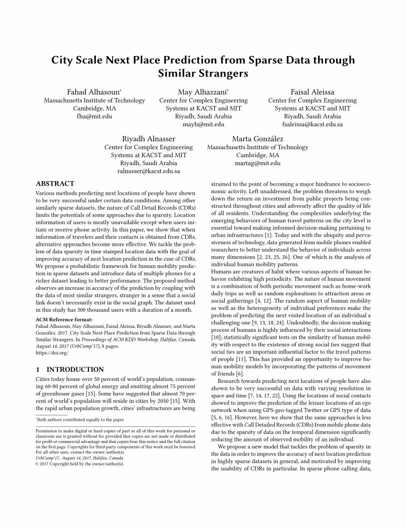
2 DATASETThe dataset for this study consists of one month of Call DetailRecords (CDRs) from the city of Riyadh in Saudi Arabia with around18 hundred towers. The data provides CDRs for the duration ofthe month of December 2012 from a major telecom operator inthe city. Phone activity for about 300 thousands users during onemonth period makes about 109 million records in the CDRs. Thespatial granularity of a cell tower varies across the city; figure 1shows the city of Riyadh and the voronoi cells of the towers inthe city, areas that are closer to the center of the city have smallercells while as we move away from the center, cells have larger sizes.Each record in the CDRs contains an anonymized user ID of thecaller and receiver, the type of communication (i.e., SMS, MMS, call,data etc), the cell tower ID facilitating the service, the duration, anda timestamp of the phone activity. Each cell tower ID is spatiallymapped to its latitude and longitude where each voronoi cell infigure 1 correspond to a tower. The data is ordered as sequencesof locations l1, l2, l3, l4, l5, l6...ln for each user i , where we have thecorresponding times for those locations as t1, t2, t3, t4, t5, t6...tn . Wealso denote the length of the sequence as Lhist and the length ofthe unique locations a user has been to as Li . For example, a userwith visit sequence of (x1,x2,x3,x1) will have Lhist = 4 and Li = 3

46.55 46.65 46.75 46.8524.55

24.65

24.75

24.85

Figure 1: Riyadh city and the coverage of cell towers.

where xi is the tower identifier. In the context of sparse datasets,individuals will have missing location information for most of thetime as discussed in the following section.

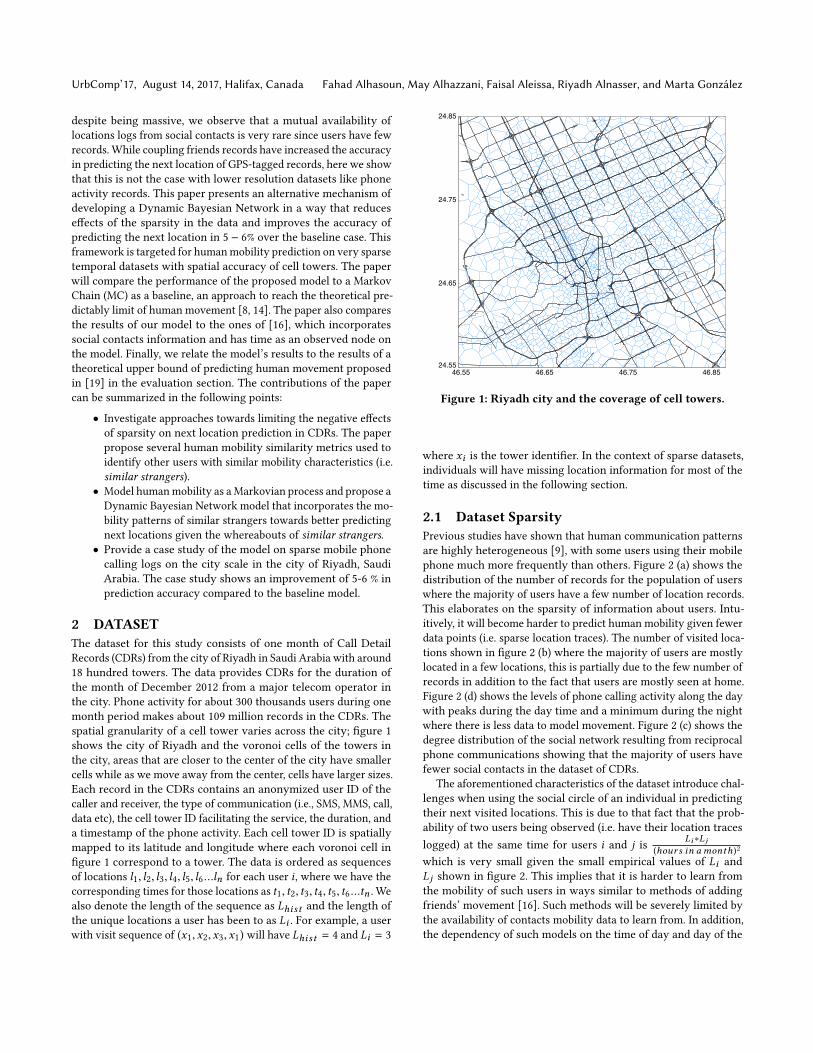
2.1 Dataset SparsityPrevious studies have shown that human communication patternsare highly heterogeneous [9], with some users using their mobilephone much more frequently than others. Figure 2 (a) shows thedistribution of the number of records for the population of userswhere the majority of users have a few number of location records.This elaborates on the sparsity of information about users. Intu-itively, it will become harder to predict human mobility given fewerdata points (i.e. sparse location traces). The number of visited loca-tions shown in figure 2 (b) where the majority of users are mostlylocated in a few locations, this is partially due to the few number ofrecords in addition to the fact that users are mostly seen at home.Figure 2 (d) shows the levels of phone calling activity along the daywith peaks during the day time and a minimum during the nightwhere there is less data to model movement. Figure 2 (c) shows thedegree distribution of the social network resulting from reciprocalphone communications showing that the majority of users havefewer social contacts in the dataset of CDRs.

The aforementioned characteristics of the dataset introduce chal-lenges when using the social circle of an individual in predictingtheir next visited locations. This is due to that fact that the prob-ability of two users being observed (i.e. have their location traceslogged) at the same time for users i and j is Li ∗Lj

(hours in amonth)2which is very small given the small empirical values of Li andLj shown in figure 2. This implies that it is harder to learn fromthe mobility of such users in ways similar to methods of addingfriends’ movement [16]. Such methods will be severely limited bythe availability of contacts mobility data to learn from. In addition,the dependency of such models on the time of day and day of the

City Scale Next Place Prediction from Sparse Data through Similar Strangers UrbComp’17, August 14, 2017, Halifax, CanadaP(

) L

hist

Length of user sequences, histLP(

N)

Number of visted locations, NP(

activ

ity)

Hour

P(d)

Degree distribution, d

A B

C D

Figure 2: The distributions of (a) Length of sequences of lo-cations Lhist and (b) Number of visited locations N and (c)Degree distribution of the social network and (d) Total activ-ity of phone usage around a typical day.

week adds more dimensions to the data which is not in the favor ofreducing the sparsity of the data.

3 TEMPORAL AND SPATIAL SIMILARITYTo overcome the discussed limitations in CDRs, we propose toadd information of users who are not necessarily within the socialcircle of the user we are modeling. Our approach is to employsimilarity measures on both the temporal and spatial dimensionsof the data to find users who will potentially help in predicting thelocation of a given user. To that end, we couple users who have themaximum temporal, spatial and spatiotemporal similarity scores;Such individuals most similar to the target user are identified asthe similar strangers in the data. We discuss each of these similaritymetrics in the following sections.

3.1 Temporal ClosenessTo gain more insight about the mobility patterns of an individualwith respect to other patterns in the population, we need to haveas much information as possible about the mobility patterns of thepopulation surrounding an individual. However, the limitation isthat it is infrequent to find location data for multiple users on thesame hour. In order to overcome this problem, we quantify how twosequences of location data overlap by a temporal closeness measure.We model the location data as two boolean vectors of length n,where n is the length of the time period in hours. Each vector cell is1 if location data for that particular hour is available and 0 otherwise.Then, we employ Russell Rao (RR) distance measure that calculates

the distance between the two vectors as follows:

RR distance =n − c11

n(1)

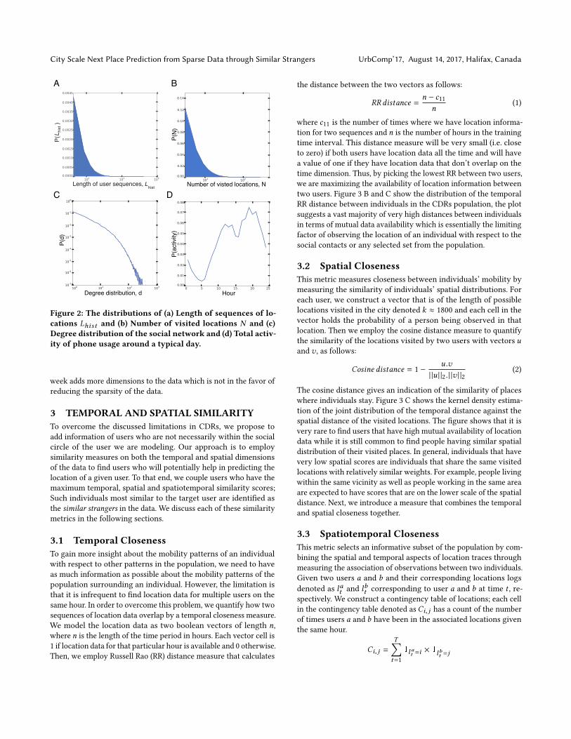
where c11 is the number of times where we have location informa-tion for two sequences and n is the number of hours in the trainingtime interval. This distance measure will be very small (i.e. closeto zero) if both users have location data all the time and will havea value of one if they have location data that don’t overlap on thetime dimension. Thus, by picking the lowest RR between two users,we are maximizing the availability of location information betweentwo users. Figure 3 B and C show the distribution of the temporalRR distance between individuals in the CDRs population, the plotsuggests a vast majority of very high distances between individualsin terms of mutual data availability which is essentially the limitingfactor of observing the location of an individual with respect to thesocial contacts or any selected set from the population.

3.2 Spatial ClosenessThis metric measures closeness between individuals’ mobility bymeasuring the similarity of individuals’ spatial distributions. Foreach user, we construct a vector that is of the length of possiblelocations visited in the city denoted k ≈ 1800 and each cell in thevector holds the probability of a person being observed in thatlocation. Then we employ the cosine distance measure to quantifythe similarity of the locations visited by two users with vectors uand v , as follows:

Cosine distance = 1 −u .v

| |u | |2.| |v | |2(2)

The cosine distance gives an indication of the similarity of placeswhere individuals stay. Figure 3 C shows the kernel density estima-tion of the joint distribution of the temporal distance against thespatial distance of the visited locations. The figure shows that it isvery rare to find users that have high mutual availability of locationdata while it is still common to find people having similar spatialdistribution of their visited places. In general, individuals that havevery low spatial scores are individuals that share the same visitedlocations with relatively similar weights. For example, people livingwithin the same vicinity as well as people working in the same areaare expected to have scores that are on the lower scale of the spatialdistance. Next, we introduce a measure that combines the temporaland spatial closeness together.

3.3 Spatiotemporal ClosenessThis metric selects an informative subset of the population by com-bining the spatial and temporal aspects of location traces throughmeasuring the association of observations between two individuals.Given two users a and b and their corresponding locations logsdenoted as lat and lbt corresponding to user a and b at time t , re-spectively. We construct a contingency table of locations; each cellin the contingency table denoted as Ci, j has a count of the numberof times users a and b have been in the associated locations giventhe same hour.

Ci, j =T∑t=1

1lat =i × 1lbt =j

UrbComp’17, August 14, 2017, Halifax, Canada Fahad Alhasoun, May Alhazzani, Faisal Aleissa, Riyadh Alnasser, and Marta González

BA C

Figure 3: Kernel density estimation of the joint distributions of ϕ distance against the RussleRao (RR) distance in (a), ϕ againstRR distance in (b) and the Cosine distance against RR in (c). The distances are calculated for every pair of users in the datasetin all three cases.

Given the contingency table, we measure the degree of associationbetween users a and b using a chi-squared test on the tableC . Then,we calculate the ϕ distance of association as follows:

ϕ = 1 −

√χ2

n(3)

Where χ2 is the chi squared test value of the contingency tableCand n is the sample of data in the table. The measure is an invertedphi coefficient where zero indicates a perfect relationship and oneindicates no relationship. This measure will have a lower distanceif users a and b move in a synchronous manner and have mutu-ally available data. Hence, the measure combines metrics discussedabove. For example, people with synchronous daily home-worktrips will have a lower spatiotemporal distance given the data tocapture that is available. Figure 3 A and B show the joint distribu-tions of the spatiotemporal distances compared to the spatial andtemporal distances discussed.

4 MODELSThe model proposed handles human mobility as a Markov pro-cess where people transition between locations with associatedprobabilities called transition probabilities. Each individual’s tran-sition between locations is intuitively related to how the rest ofthe population is moving in an urban setting. The model aims atutilizing such information to better predict human movement in theCDRs. This section will describe a baseline model and our improvedmethodology using a Dynamic Bayesian Network (DBN) incorpo-rating the mobility information of users with similar behavior orsimilar strangers that we quantify using the closeness measures wedefined in the previous section.

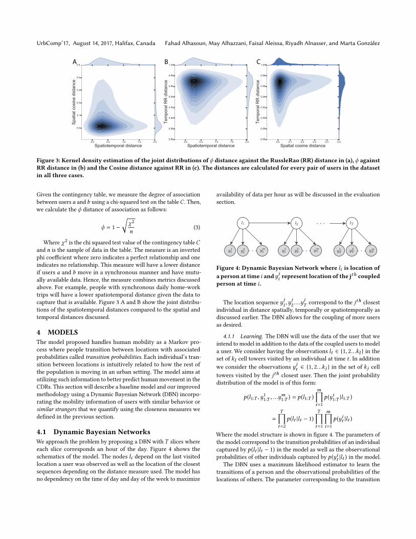
4.1 Dynamic Bayesian NetworksWe approach the problem by proposing a DBN with T slices whereeach slice corresponds an hour of the day. Figure 4 shows theschematics of the model. The nodes li depend on the last visitedlocation a user was observed as well as the location of the closestsequences depending on the distance measure used. The model hasno dependency on the time of day and day of the week to maximize

availability of data per hour as will be discussed in the evaluationsection.

. . .

. . .. . . . . .

l1 l2

y11 y1

2y21 y2

2 ym2ym

1

lT

y1T y2

T ymT

Figure 4: Dynamic Bayesian Network where li is location ofa person at time i andy ji represent location of the jth coupledperson at time i.

The location sequence y j1,yj2....y

jT correspond to the jth closest

individual in distance spatially, temporally or spatiotemporally asdiscussed earlier. The DBN allows for the coupling of more usersas desired.

4.1.1 Learning. The DBN will use the data of the user that weintend to model in addition to the data of the coupled users to modela user. We consider having the observations lt ∈ {1, 2...kl } in theset of kl cell towers visited by an individual at time t . In additionwe consider the observations y jt ∈ {1, 2...kj } in the set of kj celltowers visited by the jth closest user. Then the joint probabilitydistribution of the model is of this form:

p (l1:T ,y11:T , ...y

m1:T ) = p (l1:T )

m∏i=1

p (yi1:T |l1:T )

=

T∏t=2

p (lt |lt − 1)T∏t=1

m∏i=1

p (yit |lt )

Where the model structure is shown in figure 4. The parameters ofthe model correspond to the transition probabilities of an individualcaptured by p (lt |lt − 1) in the model as well as the observationalprobabilities of other individuals captured by p (yit |lt ) in the model.

The DBN uses a maximum likelihood estimator to learn thetransitions of a person and the observational probabilities of thelocations of others. The parameter corresponding to the transition

City Scale Next Place Prediction from Sparse Data through Similar Strangers UrbComp’17, August 14, 2017, Halifax, Canada

probabilities is a matrix of size kl × kl where each cell correspondsto the transition probability between two places.

Tr (a,b) = p (lt = a |lt−1 = b)

Where Tr is the transition probability matrix of size kl × kl .In addition, the DBN learns the conditional probabilities of thelocation of a user given their similar strangers using a maximumlikelihood estimator as well. The model will learnm observationalmatrices each corresponding to a couple of the user and similarstranger i:

Obi (a,k ) = p (yit = a |lt = k ) f or i = 1...m

Where Obi is a kj × kl matrix.

4.1.2 Inference. After the DBN learns the transitions and ob-servational probabilities, we then can infer the most probable nextlocations. To get the most probable sequence of locations visitedgiven the locations of the most similar strangers at different times ofthe day, we use a MAP estimator to find l∗1:t by finding the argmaxin the following:

l∗1:t = argmaxl1:t

p (l1:t |y11:t , ...y

m1:t )

Where the predicted locations depend on the parameter Tr (a,b) oftransition probabilities between locations a to b and the parametersfor the observational probabilities Obi for each similar stranger.

4.2 Markov Chains (Baseline Model)The model developed by Lu et al. shows that a Markov Chainapproaches the limits of predictability in human mobility usingmobile phone data of a user alone, we will use the model as thebaseline model in this paper. The Markov Chain is similar to theemployed DBN where we consider having the observations lt ∈{1, 2...kl } in the set of kl cell towers visited by an individual attime t . However, the approach doesn’t make use of social contactsor similar strangers mobility patterns. The Markov Chain onlylearns from individuals historical records and thus doesn’t coupleinformation of others. The joint probability of the model is givenby:

p (l1:T ) =T∏t=2

p (lt |lt−1)

The Markov Chain learns the transition probability matrix of sizekl × kl where each cell corresponds to the transition probabilitybetween places:

p (lt = a |lt−1 = b) = Tr (a,b)

Similar to the DBN model, Tr is a transition probability matrix ofsize kl × kl estimated using a maximum likelihood estimator.

Using the learned parameters, we use a MAP estimator to esti-mate the most probable locations by looking for the sequence thathas the highest probability l∗1:t .

l∗1:t = argmaxl1:t

p (l1:t ) = argmaxl1:t

t∏i=2

p (lt |lt − 1)

Hence, the baseline model only uses transition probabilities toestimate the most probable sequence of locations l∗1:t .

5 EVALUATIONIn order to evaluate the proposed methodology, we compare theaccuracy with existing methods of coupling with social contacts[16] as well as the Markov Chain baseline model described above.The accuracy of the model is given by:

accuracy =

T∑t=1

1lt=l ∗t

T

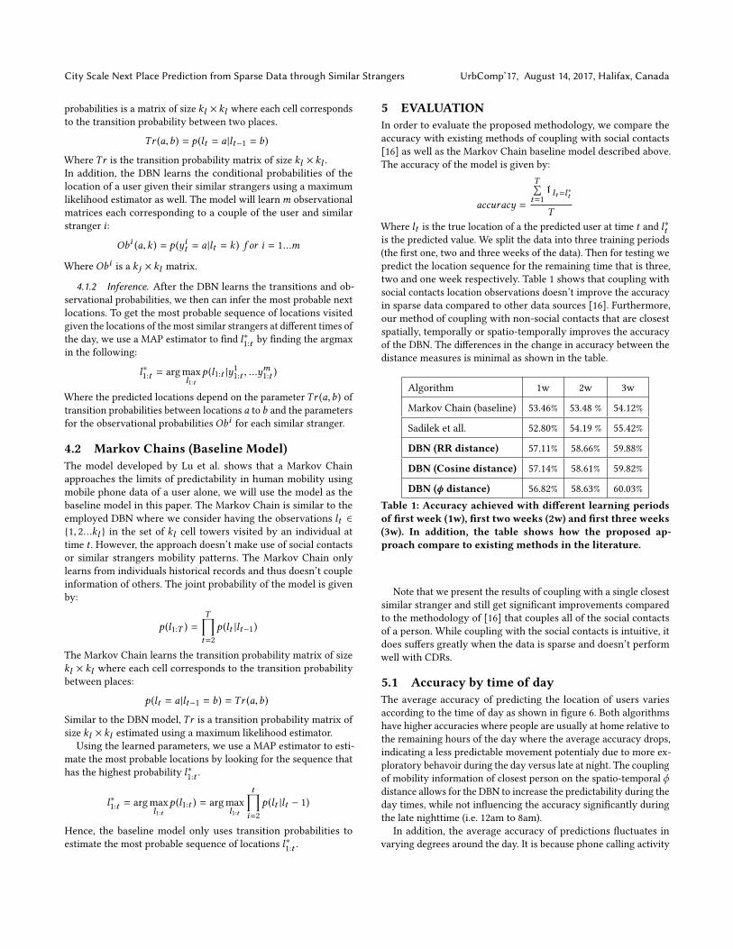
Where lt is the true location of a the predicted user at time t and l∗tis the predicted value. We split the data into three training periods(the first one, two and three weeks of the data). Then for testing wepredict the location sequence for the remaining time that is three,two and one week respectively. Table 1 shows that coupling withsocial contacts location observations doesn’t improve the accuracyin sparse data compared to other data sources [16]. Furthermore,our method of coupling with non-social contacts that are closestspatially, temporally or spatio-temporally improves the accuracyof the DBN. The differences in the change in accuracy between thedistance measures is minimal as shown in the table.

Algorithm 1w 2w 3w

Markov Chain (baseline) 53.46% 53.48 % 54.12%

Sadilek et all. 52.80% 54.19 % 55.42%

DBN (RR distance) 57.11% 58.66% 59.88%

DBN (Cosine distance) 57.14% 58.61% 59.82%

DBN (ϕ distance) 56.82% 58.63% 60.03%Table 1: Accuracy achieved with different learning periodsof first week (1w), first two weeks (2w) and first three weeks(3w). In addition, the table shows how the proposed ap-proach compare to existing methods in the literature.

Note that we present the results of coupling with a single closestsimilar stranger and still get significant improvements comparedto the methodology of [16] that couples all of the social contactsof a person. While coupling with the social contacts is intuitive, itdoes suffers greatly when the data is sparse and doesn’t performwell with CDRs.

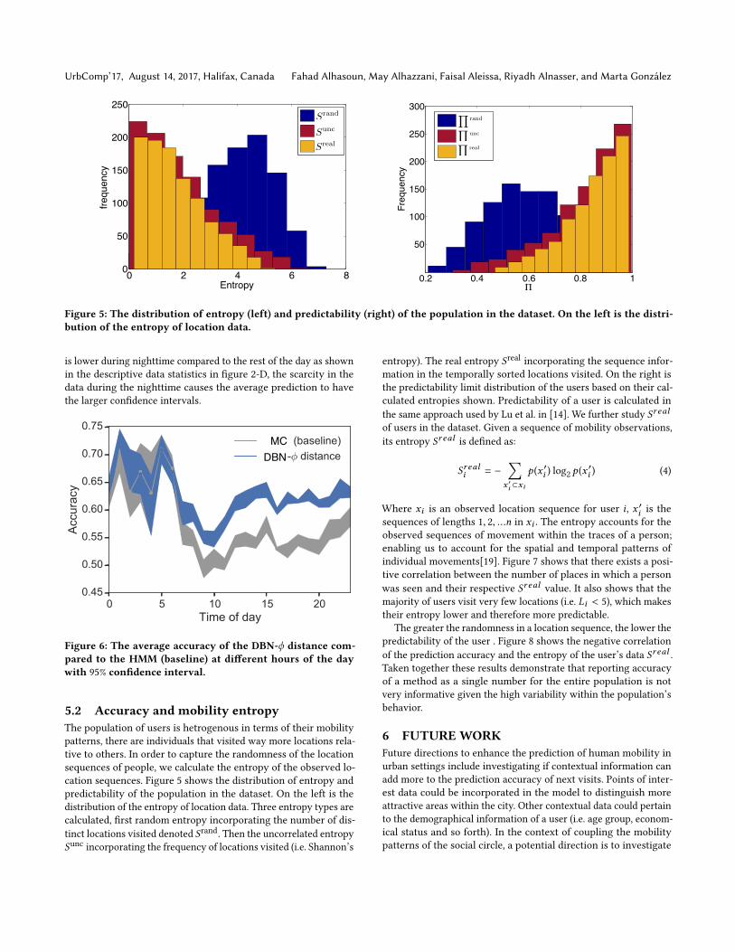
5.1 Accuracy by time of dayThe average accuracy of predicting the location of users variesaccording to the time of day as shown in figure 6. Both algorithmshave higher accuracies where people are usually at home relative tothe remaining hours of the day where the average accuracy drops,indicating a less predictable movement potentialy due to more ex-ploratory behavoir during the day versus late at night. The couplingof mobility information of closest person on the spatio-temporal ϕdistance allows for the DBN to increase the predictability during theday times, while not influencing the accuracy significantly duringthe late nighttime (i.e. 12am to 8am).

In addition, the average accuracy of predictions fluctuates invarying degrees around the day. It is because phone calling activity

UrbComp’17, August 14, 2017, Halifax, Canada Fahad Alhasoun, May Alhazzani, Faisal Aleissa, Riyadh Alnasser, and Marta González100 101 10210−7

10−6

10−5

10−4

10−3

10−2

10−1

100

Li

P(L i)

L100 101 102 103

10−7

10−6

10−5

10−4

10−3

10−2

10−1

100

P(L hist)

histL

0 2 4 6 80

50

100

150

200

250

Entropy

frequency

Srand

Sunc

Sreal

0.2 0.4 0.6 0.8 1

50

100

150

200

250

300

W

Freq

uenc

y

W rand

W uncW max

Yrand

Yunc

YrealSreal

Sunc

Srand

Figure 5: The distribution of entropy (left) and predictability (right) of the population in the dataset. On the left is the distri-bution of the entropy of location data.

is lower during nighttime compared to the rest of the day as shownin the descriptive data statistics in figure 2-D, the scarcity in thedata during the nighttime causes the average prediction to havethe larger confidence intervals.

MCDBN

Figure 6: The average accuracy of the DBN-ϕ distance com-pared to the HMM (baseline) at different hours of the daywith 95% confidence interval.

5.2 Accuracy and mobility entropyThe population of users is hetrogenous in terms of their mobilitypatterns, there are individuals that visited way more locations rela-tive to others. In order to capture the randomness of the locationsequences of people, we calculate the entropy of the observed lo-cation sequences. Figure 5 shows the distribution of entropy andpredictability of the population in the dataset. On the left is thedistribution of the entropy of location data. Three entropy types arecalculated, first random entropy incorporating the number of dis-tinct locations visited denoted Srand. Then the uncorrelated entropySunc incorporating the frequency of locations visited (i.e. Shannon’s

entropy). The real entropy Sreal incorporating the sequence infor-mation in the temporally sorted locations visited. On the right isthe predictability limit distribution of the users based on their cal-culated entropies shown. Predictability of a user is calculated inthe same approach used by Lu et al. in [14]. We further study Sr ealof users in the dataset. Given a sequence of mobility observations,its entropy Sr eal is defined as:

Sr eali = −∑x ′i ⊂xi

p (x ′i ) log2 p (x′i ) (4)

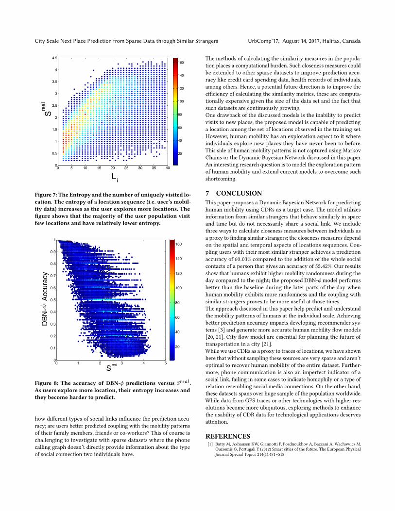
Where xi is an observed location sequence for user i , x ′i is thesequences of lengths 1, 2, ...n in xi . The entropy accounts for theobserved sequences of movement within the traces of a person;enabling us to account for the spatial and temporal patterns ofindividual movements[19]. Figure 7 shows that there exists a posi-tive correlation between the number of places in which a personwas seen and their respective Sr eal value. It also shows that themajority of users visit very few locations (i.e. Li < 5), which makestheir entropy lower and therefore more predictable.

The greater the randomness in a location sequence, the lower thepredictability of the user . Figure 8 shows the negative correlationof the prediction accuracy and the entropy of the user’s data Sr eal .Taken together these results demonstrate that reporting accuracyof a method as a single number for the entire population is notvery informative given the high variability within the population’sbehavior.

6 FUTUREWORKFuture directions to enhance the prediction of human mobility inurban settings include investigating if contextual information canadd more to the prediction accuracy of next visits. Points of inter-est data could be incorporated in the model to distinguish moreattractive areas within the city. Other contextual data could pertainto the demographical information of a user (i.e. age group, econom-ical status and so forth). In the context of coupling the mobilitypatterns of the social circle, a potential direction is to investigate

City Scale Next Place Prediction from Sparse Data through Similar Strangers UrbComp’17, August 14, 2017, Halifax, Canada

0 5 10 15 20 25 30 35 400

0.5

1

1.5

2

2.5

3

3.5

4

4.5

Li

Sreal

20

40

60

80

100

120

140

160

20

40

60

80

100

120

140

160

Figure 7: The Entropy and the number of uniquely visited lo-cation. The entropy of a location sequence (i.e. user’s mobil-ity data) increases as the user explores more locations. Thefigure shows that the majority of the user population visitfew locations and have relatively lower entropy.

0 1 2 3 4 50

0.1

0.2

0.3

0.4

0.5

0.6

0.7

0.8

0.9

1

DBN-

A

ccur

acy

S real

20

40

60

80

100

120

140

160

Figure 8: The accuracy of DBN-ϕ predictions versus Sr eal .As users explore more location, their entropy increases andthey become harder to predict.

how different types of social links influence the prediction accu-racy; are users better predicted coupling with the mobility patternsof their family members, friends or co-workers? This of course ischallenging to investigate with sparse datasets where the phonecalling graph doesn’t directly provide information about the typeof social connection two individuals have.

The methods of calculating the similarity measures in the popula-tion places a computational burden. Such closeness measures couldbe extended to other sparse datasets to improve prediction accu-racy like credit card spending data, health records of individuals,among others. Hence, a potential future direction is to improve theefficiency of calculating the similarity metrics, these are computa-tionally expensive given the size of the data set and the fact thatsuch datasets are continuously growing.One drawback of the discussed models is the inability to predictvisits to new places, the proposed model is capable of predictinga location among the set of locations observed in the training set.However, human mobility has an exploration aspect to it whereindividuals explore new places they have never been to before.This side of human mobility patterns is not captured using MarkovChains or the Dynamic Bayesian Network discussed in this paper.An interesting research question is to model the exploration patternof human mobility and extend current models to overcome suchshortcoming.

7 CONCLUSIONThis paper proposes a Dynamic Bayesian Network for predictinghuman mobility using CDRs as a target case. The model utilizesinformation from similar strangers that behave similarly in spaceand time but do not necessarily share a social link. We includethree ways to calculate closeness measures between individuals asa proxy to finding similar strangers; the closeness measures dependon the spatial and temporal aspects of locations sequences. Cou-pling users with their most similar stranger achieves a predictionaccuracy of 60.03% compared to the addition of the whole socialcontacts of a person that gives an accuracy of 55.42%. Our resultsshow that humans exhibit higher mobility randomness during theday compared to the night; the proposed DBN-ϕ model performsbetter than the baseline during the later parts of the day whenhuman mobility exhibits more randomness and the coupling withsimilar strangers proves to be more useful at those times.The approach discussed in this paper help predict and understandthe mobility patterns of humans at the individual scale. Achievingbetter prediction accuracy impacts developing recommender sys-tems [3] and generate more accurate human mobility flow models[20, 21]. City flow model are essential for planning the future oftransportation in a city [21].While we use CDRs as a proxy to traces of locations, we have shownhere that without sampling these sources are very sparse and aren’toptimal to recover human mobility of the entire dataset. Further-more, phone communication is also an imperfect indicator of asocial link, failing in some cases to indicate homophily or a type ofrelation resembling social media connections. On the other hand,these datasets spans over huge sample of the population worldwide.While data from GPS traces or other technologies with higher res-olutions become more ubiquitous, exploring methods to enhancethe usability of CDR data for technological applications deservesattention.

REFERENCES[1] Batty M, Axhausen KW, Giannotti F, Pozdnoukhov A, Bazzani A, Wachowicz M,

Ouzounis G, Portugali Y (2012) Smart cities of the future. The European PhysicalJournal Special Topics 214(1):481–518

UrbComp’17, August 14, 2017, Halifax, Canada Fahad Alhasoun, May Alhazzani, Faisal Aleissa, Riyadh Alnasser, and Marta González

[2] Blondel VD, Decuyper A, Krings G (2015) A survey of results on mobile phonedatasets analysis. arXiv preprint arXiv:150203406

[3] Borras J, Moreno A, Valls A (2014) Intelligent tourism recommender systems: Asurvey. Expert Systems with Applications 41(16):7370–7389

[4] Cho E, Myers SA, Leskovec J (2011) Friendship and mobility: user movementin location-based social networks. In: Proceedings of the 17th ACM SIGKDDinternational conference on Knowledge discovery and data mining, ACM, pp1082–1090

[5] DashM, Koo KK, Gomes JB, Krishnaswamy SP, Rugeles D, Shi-Nash A (2015) Nextplace prediction by understanding mobility patterns. In: Pervasive Computingand Communication Workshops (PerCom Workshops), 2015 IEEE InternationalConference on, IEEE, pp 469–474

[6] De Domenico M, Lima A, Musolesi M (2013) Interdependence and predictabilityof human mobility and social interactions. Pervasive and Mobile Computing9(6):798–807

[7] Eagle N, Clauset A, Quinn JA (2009) Location segmentation, inference and pre-diction for anticipatory computing. In: AAAI Spring Symposium: TechnosocialPredictive Analytics, pp 20–25

[8] Gambs S, Killijian MO, del Prado Cortez MN (2012) Next place prediction usingmobility markov chains. In: Proceedings of the First Workshop on Measurement,Privacy, and Mobility, ACM, p 3

[9] González MC, Hidalgo CA, Barabasi AL (2008) Understanding individual humanmobility patterns. Nature 453(7196):779–782

[10] Granovetter M (1985) Economic action and social structure: the problem ofembeddedness. American journal of sociology pp 481–510

[11] Jameson L Toole CS C Herrera-YagÃije, González MC (2015) Coupled mobility ofsocial ties. Journal of the Royal Society Interface

[12] Jiang S, Yang Y, Gupta S, Veneziano D, Athavale S, González MC (2016) Thetimegeo modeling framework for urban motility without travel surveys. Proceed-ings of the National Academy of Sciences p 201524261

[13] Liao L, Patterson DJ, Fox D, Kautz H (2007) Learning and inferring transportationroutines. Artificial Intelligence 171(5):311–331

[14] Lu X, Wetter E, Bharti N, Tatem AJ, Bengtsson L (2013) Approaching the limit ofpredictability in human mobility. Scientific reports 3

[15] Rode P, Burdett R (2011) Cities: investing in energy and resource efficiency[16] Sadilek A, Kautz H, Bigham JP (2012) Finding your friends and following them

to where you are. In: Proceedings of the fifth ACM international conference onWeb search and data mining, ACM, pp 723–732

[17] Scellato S, Musolesi M, Mascolo C, Latora V, Campbell AT (2011) Nextplace:a spatio-temporal prediction framework for pervasive systems. In: PervasiveComputing, Springer, pp 152–169

[18] Schneider CM, Belik V, Couronné T, Smoreda Z, González MC (2013) Unrav-elling daily human mobility motifs. Journal of The Royal Society Interface10(84):20130,246

[19] Song C, Qu Z, Blumm N, Barabási AL (2010) Limits of predictability in humanmobility. Science 327(5968):1018–1021

[20] Toole JL, Colak S, Alhasoun F, Evsukoff A, González MC (2014) The path mosttravelled: mining road usage patterns from massive call data. arXiv preprintarXiv:14030636

[21] Wang P, Hunter T, Bayen AM, Schechtner K, González MC (2012) Understandingroad usage patterns in urban areas. Scientific reports 2

[22] Wei LY, Zheng Y, Peng WC (2012) Constructing popular routes from uncertaintrajectories. In: Proceedings of the 18th ACM SIGKDD international conferenceon Knowledge discovery and data mining, ACM, pp 195–203

[23] Ye Y, Zheng Y, Chen Y, Feng J, Xie X (2009) Mining individual life pattern based onlocation history. In: Mobile Data Management: Systems, Services andMiddleware,2009. MDM’09. Tenth International Conference on, IEEE, pp 1–10

[24] Zheng Y, Zhou X (2011) Computing with spatial trajectories. Springer Science &Business Media

[25] Zheng Y, Capra L, Wolfson O, Yang H (2014) Urban computing: concepts, method-ologies, and applications. ACM Transactions on Intelligent Systems and Technol-ogy (TIST) 5(3):38

[26] Zheng Y, Capra L, Wolfson O, Yang H (2014) Urban computing: concepts, method-ologies, and applications. ACM Transactions on Intelligent Systems and Technol-ogy (TIST) 5(3):38