Embed Size (px)
Citation preview

Galvao Jr, A. F., Montes-Rojas, G. & Park, S. Y. (2013). Quantile Autoregressive Distributed Lag
Model with an Application to House Price Returns. Oxford Bulletin of Economics and Statistics,
75(2), pp. 307-321. doi: 10.1111/j.1468-0084.2011.00683.x
City Research Online
Original citation: Galvao Jr, A. F., Montes-Rojas, G. & Park, S. Y. (2013). Quantile Autoregressive
Distributed Lag Model with an Application to House Price Returns. Oxford Bulletin of Economics
and Statistics, 75(2), pp. 307-321. doi: 10.1111/j.1468-0084.2011.00683.x
Permanent City Research Online URL: http://openaccess.city.ac.uk/12039/
Copyright & reuse
City University London has developed City Research Online so that its users may access the
research outputs of City University London's staff. Copyright © and Moral Rights for this paper are
retained by the individual author(s) and/ or other copyright holders. All material in City Research
Online is checked for eligibility for copyright before being made available in the live archive. URLs
from City Research Online may be freely distributed and linked to from other web pages.
Versions of research
The version in City Research Online may differ from the final published version. Users are advised
to check the Permanent City Research Online URL above for the status of the paper.
Enquiries
If you have any enquiries about any aspect of City Research Online, or if you wish to make contact
with the author(s) of this paper, please email the team at [email protected].
Quantile autoregressive distributed lag model
with an application to house price returns∗
ANTONIO F. GALVAO, JR.† GABRIEL MONTES-ROJAS‡
SUNG Y. PARK§
†Department of Economics, The University of Iowa, Iowa City, IA 52242, USA (e-mail:[email protected])
‡Department of Economics, City University London, London EC1V 0HB, UK (e-mail:[email protected])
§Department of Economics, The Chinese University of Hong Kong,Shatin, N.T., HongKong (e-mail: [email protected])
Abstract
This paper studies quantile regression in an autoregressive dynamic framework withexogenous stationary covariates. We demonstrate the potential of the quantile autore-gressive distributed lag model with an application to house price returns in the UnitedKingdom. The results show that house price returns present a heterogeneous autore-gressive behavior across the quantiles. The real GDP growth and interest rates alsohave an asymmetric impact on house prices variations.
Key Words: quantile autoregression, distributed lag model, autoregressive model
JEL Classification: C14; C32
∗The authors would like to express their appreciation to Christopher Adam, two anonymous referees, DanBernhardt, Odilon Camara, Roger Koenker, Luiz Lima, Simone Manganelli and the participants of seminarsat University of Wisconsin-Milwaukee and the 2008 XMU-HUB Workshop on Economics and FinancialEconometrics for helpful comments and discussions. All the remaining errors are ours.

I. Introduction
Asymmetric dynamic responses are common in the time series empirical literature. For
instance, Beaudry and Koop (1993) show that positive shocks to the U.S. GDP are more
persistent than negative shocks. Poterba (1991) and Capozza et al. (2002) among others,
present evidence on the asymmetric responses of house prices to income shocks. The occur-
rence of these asymmetries call into question the usefulness of models with time invariant
structures as means of modeling such series. Quantile regression (QR) is a statistical method
for estimating models of conditional quantile functions, which offers a systematic strategy for
examining how covariates influence the location, scale, and shape of the entire response dis-
tribution, therefore exposing a variety of heterogeneity in response dynamics. Koenker and
Xiao (2006) introduced quantile autoregression (QAR) models in which the autoregressive
coefficients can be expressed as monotone functions of a single, scalar random variable. QAR
models are becoming increasingly popular, and there is a growing literature about estimation
of QR models for time series. Engle and Manganelli (2004) propose a quantile autoregres-
sive framework to model value-at-risk where the quantiles follow an autoregressive process.
Gourieroux and Jasiak (2008) study dynamic additive quantile model. Xiao (2009) proposes
QR with cointegrated time series. Recently, Xiao and Koenker (2009) studied conditional
quantiles for GARCH models using QR.1
The purpose of this paper is to generalize the Koenker and Xiao (2006) QAR framework
introducing exogenous stationary covariates and to provide an application to illustrate the
usefulness of the new model to study asymmetric behavior in time series. We develop a
quantile autoregressive distributed lag (QADL) model. The QADL model can deliver im-
portant insights about asymmetric dynamics, such as heterogeneous adjustments in time
1Koenker and Xiao (2004) study statistical inference in QAR models when the largest autoregressivecoefficient may be unity. Galvao (2009) develops tests for unit roots allowing for stationary covariates anda linear time trend into the quantile autoregression model.
1
series models where controlling for lagged regressors and exogenous covariates is important.
The approach proposed in this paper is different from that of Engle and Manganelli (2004)
because we use QR in the standard linear time series context, modeling the conditional
quantile function as linear and depending on past values of the dependent variable, instead
of modeling the quantile functions themselves as an autoregressive process. This reduces the
computational burden substantially. Moreover, the QADL model allows for some forms of
explosive behavior in some quantiles while maintaining stationarity of the process, as long
as certain stationarity conditions are satisfied on the whole distribution, while Engle and
Manganelli (2004) exclude this case.2
Note that QAR and QADL in time series have a different interpretation than that of
QR in cross-sectional data. In general, QR shows how a given quantile of the conditional
distribution of y depends on the covariates x. In the cross-sectional case, this can be in-
terpreted as the different effects that covariates exert on a given outcome for individuals on
that corresponding quantile of the conditional distribution. In a time series context, how-
ever, we estimate the conditional quantile function of a particular variable along time, for
instance aggregated variables such as GDP and consumption, index numbers, or as in the
illustration presented in the paper house price returns. Then, we interpret the conditional
quantiles function at a given time as different phases of the business cycle, where low and
high quantiles of the conditional distribution of price returns corresponds to periods of de-
clining and increasing prices respectively. This interpretation might also be used for output
gap, consumption growth or value-at-risk applications.
We illustrate the QADL model with an application to quarterly house price returns data
in the United Kingdom (UK). House prices volatility has claimed unprecedented importance
and there is a growing literature on this topic (for instance Muellbauer and Murphy, 1997;
2We do not consider the Xiao (2009) case where the variables are cointegrated, but rather we consider anexogenous set of stationary covariates.
2

Ortalo-Magne and Rady, 1999, 2006; Rosenthal, 2006). We argue that QR can be used to de-
scribe the asymmetric responses of house prices returns to income and interest rates shocks.
We interpret the conditional quantile functions as different phases of the market. High quan-
tiles correspond to a phase of unusually high conditional returns; while low quantiles to low
conditional returns. The results show that house price returns have an asymmetric autore-
gressive behavior, and that real GDP growth and interest rates have an asymmetric impact on
house prices returns along the quantiles. In addition, the results suggest high autoregressive
persistence in the extreme high quantiles. However, unit root tests reject the null hypothesis
of unit root on house price returns. Thus, the model seems to show global stationarity with
some persistence in unusually high returns. The inclusion of stationary covariates reduces
the asymmetric autoregressive responses but maintains the persistence in the high quantiles.
The interest rates have a negative impact on house prices returns, mostly significant for low
quantiles. This can be interpreted as the fact that the interest rates have an effect on stimu-
lating the demand in the real estate market when returns are low, but it does not deter house
prices booms. In addition, there is evidence that the impact of GDP on house prices presents
an asymmetric impact and it is stronger for low and high quantiles. For low quantiles, this is
interpreted as the fact that GDP growth reactivates the real estate market when returns are
low, while it might be contributing to house prices’ busts (as that in the early 1990’s where a
recession was accompanied by a significant decline in house prices). Moreover, it contributes
to sustaining house prices booms. In other words, periods of unusually high (conditional)
returns are very responsive to GDP growth. In this case, the conditional mean may be a
misleading estimator in periods of low and high conditional returns, which are those when
policymakers are more keen to intervene or to predict future behavior.
The rest of the paper is organized as follows. Section 2 presents the model, describes
the estimator and its asymptotic properties. Section 3 presents some Monte Carlo evidence.
3

In Section 4 we illustrate the new approach by applying it to a house price returns dataset.
Finally, Section 5 concludes the paper.
II. QADL: model, estimation and inference
The autoregressive-distributed lag model is described by the following equation
yt = µ +
p∑
j=1
αjyt−j +
q∑
l=0
x′t−lθl + εt; t = 1, ..., n (1)
where yt is the response variable, yt−j is the lag of the response variable, xt is a dim(x)-
dimensional vector of covariates and εt is the innovation.3 The main aim of this type of model
is to emphasize alternative short-run dynamic structures. In addition, this class of models
also provides important long-run results that are of particular interest for inference about
the validity of a proposed economic theory. Nevertheless, the least squares models might be
insufficient to describe heterogeneity in the impact of the shocks in a given time series.
As in Koenker and Xiao (2006), let Ut be a sequence of independent and identi-
cally distributed (i.i.d.) standard uniform random variables, and consider the following
autoregressive-distributed lag process
yt = µ (Ut) +
p∑
j=1
αj (Ut) yt−j +
q∑
l=0
x′t−lθl (Ut) (2)
where α and θ are unknown functions [0,1]→ R that we want to estimate. Given that the
right hand side of (2) is monotone increasing on Ut, it follows that the τ -th conditional
quantile function of yt can be written as
Qyt(τ |ℑt) = µ (τ) +
p∑
j=1
αj (τ) yt−j +
q∑
l=0
x′t−qθl (τ) (3)
3We assume, for convenience, that each variable in xt have the same lag truncation, q. The case ofdifferent lag truncation for each variable is immediate.
4

where ℑt is the σ-field generated by ys, xs, s ≤ t.4 We refer to model (3) as the quantile
autoregressive distributed-lag of orders p and q (QADL(p, q)). Implicitly in the formulation
of model (3) is the requirement that Qyt(τ |ℑt) is monotone increasing in τ for all ℑt. A more
compact notation to describe model (3) is
Qyt(τ |ℑt) = z′tβ(τ) (4)
where zt = (1, yt−1, ..., yt−p, xt, ..., xt−q)′ and β(τ) = (µ (τ) , α1 (τ) , ..., αp (τ) , θ′0 (τ) , ..., θ′q (τ))′.
It is important to emphasize that monotonicity of the conditional quantile functions
imposes some discipline on the forms taken by the coefficients. It requires that the function
Qyt(τ |ℑt) is monotone in τ in a relevant region of the ℑt-space. In some circumstances,
this necessitates restricting the domain of the dependent variables; in others, when the
coordinates of the dependent variables are themselves functionally dependent, monotonicity
may hold globally. The estimated conditional quantile function Qyt(τ |ℑt) = z′tβ(τ) is ensured
to be monotone in τ at zt = z, as noted in Koenker and Xiao (2006). However, this does
not guarantee that it will be monotone in τ for other values of z. Furthermore, because
we are using a linear model, there must be crossing sufficiently far away from z. It may be
that such crossing occurs outside the convex hull of the z observations, in which case the
estimated model may be viewed as an adequate approximation within this region. But it
is not unusual to find that the crossing has occurred in this region as well.5 As discussed
in Koenker and Xiao (2006), one can find a linear reparametrization of the model that does
exhibit co-monotonicity over some relevant region of covariate space. Recently, Gourieroux
4The transition from (2) to (3) is an immediate consequence of the fact that for any monotone increasingfunction g and standard uniform random variable, U , we have Qg(U)(τ) = g(QU (τ)) = g(τ), where QU (τ) = τis the quantile function of U .
5It is easy to check whether Qyt(τ |ℑt) is monotone at particular z points. To verify monotonicity for
a given z, one may compute this for several quantiles, and plot it against the sequence of τ . If there is asignificant number of observed points at which this condition is violated, then this can be taken as evidence ofmodel misspecification. Failure of the monotonicity condition might also imply that the conditional quantilefunctions are not linear. In this paper, we assume that monotonicity of Qyt
(τ |ℑt) in τ , for some relevantregion of ℑt-space, holds. We refer the reader to Gourieroux and Jasiak (2008), Neocleous and Portnoy(2008), Koenker and Xiao (2006), and Koenker (2005) for more details about monotonicity in QR.
5

and Jasiak (2008) propose a dynamic additive quantile model that ensures the monotonicity
of conditional quantile estimates.
The estimation procedure is based on standard linear quantile regression. Thus, estima-
tion of the QADL model (3) involves solving the following problem
minβ∈ℜ1+p+(1+q)×dim(x)
n∑
t=1
ρτ (yt − z′tβ) (5)
where ρτ (u) = u(τ − I(u < 0)), as in Koenker and Bassett (1978). The details of the
proofs for consistency and asymptotic normality of the estimator, β(τ), are provided in
Galvao et al. (2009). Define the following elements: Ω0 = E(ztz′t) = lim n−1
∑n
t=1 ztz′t, and
Ω1(τ) = lim n−1∑n
t=1 ft−1[F−1t−1(τ)]ztz
′t, and let Σ(τ) = Ω1(τ)−1Ω0Ω1(τ)−1. The limiting
distribution of the QADL estimator for a fixed quantile τ is
√n
(
β(τ) − β(τ))
d→ N(0, τ(1 − τ)Σ(τ)).
In order to make appropriate inference it is necessary to estimate Σ(τ) consistently. Since
Ω0 involves no nuisance parameter it can easily be estimated as Ω0(τ) = 1n
∑n
t=1 ztz′t. Let
ut(τ) = yt − z′tβ(τ), in order to estimate the matrix Ω1(τ), we follow Powell (1986)
Ω1(τ) =1
2nhn
n∑
t=1
I(|ut(τ)| ≤ hn)ztz′t,
where hn is an appropriately chosen bandwidth, with hn → 0 and nh2n → ∞.6
In model (3) the choice of p and q is important. In order to select appropriate models
we suggest the use of BIC criteria, adapted to QADL along the lines suggested by Machado
(1993), which is based on the Asymmetric Laplace Distribution. At the median it uses the
criterion
BIC = n log σ +1 + p + (1 + q) × dim(x)
2log n
6In the simulations and application, we consider the default bandwidth suggested by Bofinger (1975),hn = [Φ−1(τ + cn) − Φ−1(τ − cn)] min(σ1, σ2), where the bandwidth cn = O(n1/3), σ1 =
√
V ar(u), and
σ2 = (Q(u, .75) − Q(u, .25))/1.34.
6

where σ = n−1∑ |yt − z′tβ(1/2)|. For other quantiles, the obvious asymmetric modification
of this expression can be used. In the example given in this paper we select the number
of lags based only on the median criterion, in order to have a comparable regression model
across quantiles. But, it is possible that there are applications in which this is not desirable.
General hypotheses tests on the vector β(τ) can be accommodated by Wald-type tests
(see Galvao et al., 2009). The Wald process and associated limiting theory provide a
natural foundation for the hypothesis Rβ(τ) = r, when r is known. Here R is a k ×
(1 + p + (1 + q)dim(x)) matrix with rank k and r is a k-dimensional vector. This formu-
lation also accommodates a wide variety of testing situations, from a simple test on single
QR coefficients to joint tests involving several parameters and distinct quantiles. Thus, for
instance, we might test for the equality of several slope coefficients across several quantiles.
Another important class of tests in the QR literature involves the Kolmogorov-Smirnov (KS)
type tests, where the interest is to examine the property of the estimator over a range of
quantiles τ ∈ T , instead of focusing only on selected quantiles. Thus, for testing Rβ(τ) = r
over τ ∈ T , one may consider the KS type sup-Wald test.
III. Monte Carlo
In this section, we briefly present simulation experiments to assess the finite sample perfor-
mance of the QADL estimator. Two simple versions of the basic model (3) are considered
in the experiments. In the first version, reported in Table 1, the scalar covariate, xt, exerts
a pure location-shift effect, and the response yt is generated by the model
yt = αyt−1 + β1xt + β2xt−1 + ut. (6)
In the second, reported in Table 2, xt exerts both location and scale effects as
yt = αyt−1 + β1xt + β2xt−1 + (γxt)ut. (7)
7

TABLE 1Location-Shift Model: Bias and RMSE of Estimators
QAR QADL OLS ADLτ 0.1 0.25 0.5 0.75 0.9 0.1 0.25 0.5 0.75 0.9 − −
N α 0.094 0.093 0.095 0.095 0.099 -0.006 -0.007 -0.008 -0.005 -0.006 0.095 -0.007(0.136) (0.126) (0.130) (0.128) (0.138) (0.087) (0.076) (0.077) (0.076) (0.086) (0.111) (0.050)
β1 0.000 -0.001 0.000 0.007 0.000 0.001(0.122) (0.109) (0.111) (0.108) (0.123) (0.072)
β2 0.006 0.006 0.006 0.000 0.010 0.005(0.131) (0.115) (0.117) (0.114) (0.129) (0.076)
t3 α 0.110 0.086 0.090 0.082 0.105 -0.007 -0.006 -0.005 -0.006 -0.009 0.098 -0.007(0.150) (0.113) (0.109) (0.111) (0.145) (0.087) (0.046) (0.045) (0.049) (0.086) (0.113) (0.050)
β1 0.000 0.001 0.001 0.001 -0.002 0.001(0.131) (0.078) (0.071) (0.080) (0.131) (0.118)
β2 0.008 0.003 0.002 0.002 0.003 0.002(0.136) (0.078) (0.075) (0.078) (0.141) (0.128)
Notes: RMSE in parenthesis. Sample size of n = 200. The number of replications is 5,000.
We employ two different distributions to generate the disturbances ut: N(0, 1) and t-
distribution with 3 degrees of freedom (t3). In all cases we set y0 = 0 and generate yt for
t = 1, ..., n according to equations (6) and (7), and in generating yt we discarded the first
100 observations, using the remaining observations for estimation. This ensures that the
results are not unduly influenced by the initial values of the y0 process. In the location case,
we generate the exogenous covariates, xt, using the same distribution as the innovations
ut. In the location-scale version, to avoid crossing, we generate covariates xt as χ23. In the
simulations, we use a sample size of n = 200, set the number of replications to 5000, and
consider the following values for the remaining parameters: (α, β1, β2) = (0.5, 0.5, 0.5) and
γ = 0.2. We compare the estimators’ coefficients in terms of bias and root mean squared
error (RMSE).7 We study four different estimators in the Monte Carlo experiments, the
QAR proposed by Koenker and Xiao (2006), the QADL proposed in this paper, the least
squares estimator (OLS), and finally, the least square distributed lag model (ADL). Finally,
we consider τ ∈ 0.1, 0.25, 0.5, 0.75, 0.9.
Table 1 shows bias and RMSE results of the estimators for the location-shift model. For
QAR and OLS models we do not include the terms xt and xt−1 in the estimating equation.
7We refer the reader to Galvao et al. (2009) for a more detailed set of results on estimation, and smallsample properties (size and power) of the Wald and Kolmogorov-Smirnov tests.
8

TABLE 2Scale-Location-Shift Model: Bias and RMSE of Estimators
QAR QADL OLS ADLτ 0.1 0.25 0.5 0.75 0.9 0.1 0.25 0.5 0.75 0.9 − −
N α 0.090 0.113 0.143 0.173 0.190 -0.005 -0.005 -0.003 -0.005 -0.008 0.144 -0.005(0.118) (0.136) (0.165) (0.192) (0.222) (0.066) (0.059) (0.060) (0.059) (0.067) (0.154) (0.042)
β1 0.009 0.004 0.002 -0.002 -0.012 0.002(0.112) (0.094) (0.093) (0.094) (0.111) (0.049)
β2 0.005 0.002 0.002 0.003 0.000 0.002(0.085) (0.075) (0.077) (0.075) (0.085) (0.053)
t3 α 0.066 0.075 0.084 0.100 0.105 -0.008 -0.006 -0.004 -0.005 -0.006 0.092 -0.008(0.102) (0.096) (0.110) (0.125) (0.153) (0.070) (0.050) (0.047) (0.045) (0.079) (0.105) (0.062)
β1 0.011 0.003 0.003 -0.005 -0.004 -0.002(0.185) (0.115) (0.106) (0.114) (0.187) (0.085)
β2 -0.005 0.001 0.001 0.005 0.012 0.006(0.137) (0.088) (0.086) (0.088) (0.136) (0.089)
Notes: RMSE in parenthesis. Sample size of n = 200. The number of replications is 5,000.
The results show that, as expected, omitting the variables in QAR and OLS cases cause bias
in estimation. However, the QADL and ADL are approximately unbiased, with the QADL
unbiased along the quantiles. The results show that for the quantile regression models the
RMSE is larger for extreme quantiles in both distributional cases. This finding shows ev-
idence that, in general, it is more difficult to estimate the variance at the extreme of the
distribution. We compare RMSE of the least squares estimators with the median quantile
regression. In the Gaussian condition, the OLS based estimators outperform the quantile
regression estimators, that is, ADL has smaller RMSEs when compared with QADL, and
OLS has smaller RMSE when compared with QAR. Finally, for the non-Gaussian case, t3,
in terms of RMSE, the median quantile regression estimators outperform their least squares
analogues. Table 2 shows bias and RMSE results of the estimates of α and β for location-
scale-shift model. In all cases the QAR and OLS are biased and the QADL and ADL are
approximately unbiased. In this case, the results regarding RMSE are qualitatively similar
to the previous case.
9
IV. Application: House Price Returns
There is an extensive literature on cross-sectional and time-series variation in house prices,
but this literature is marked by poor predictability. Mankiew and Weil (1989) find that the
Baby Boom had a large impact on the US housing market. By 1989 they predicted a future
slow down in the house market, which was not observed.8 In fact, house prices have shown
unprecedented values over the past 10 years. Increasing house prices had also importance
in the UK. The issue of affordable housing had claimed an increasing importance in the
public debate and the uncertainty about future prices is a concern of both policy makers
and researchers.9 Moreover, the fact that housing is a major component of wealth (Banks
and Tanner, 2002, show that real state accounted for 35% of aggregate household wealth in
the UK in the 1990s) and risky assets determines that house price changes have significant
effects on aggregate consumption (see for instance Campbell and Cocco, 2007).
The evolution of house prices was extensively studied in the UK by Muellbauer and
Murphy (1997), Ortalo-Magne and Rady (1999, 2006) and Rosenthal (2006) among others.
Those authors rigorously studied the booms and busts in the UK housing market until 2000.
In the past 50 years, there have been three major booms in the UK’s owner-occupied housing
market: in the early 1970s, in the late 1980s and the current housing boom. There were also
smaller booms in the 1960s and, more briefly, in the late 1970s, while the early 1990s saw a
bust on an unprecedented scale. Many factors conspired to produce the house price boom
of the late 1980s. Initial debt levels were low as were real house prices, giving scope for rises
in both. Income growth after the early 1980s recession was strong, as were income growth
expectations and these became more important as a result of financial liberalization, though
8“Our estimates suggest that real housing prices will fall substantially - indeed, real housing prices maywell reach levels lower than those experienced at any time in the past forty years.” (p.236)
9‘Our forecasts have not been for dramatic falls in house prices, but who knows?... anyone who thinksthat they can forecast asset prices is kidding themselves’. Rachel Lomax, Governor of Bank of England, TheGuardian, London, November 23, 2003, cited in Rosenthal (2006, p. 289).
10

partly offset by bigger real interest rate effects. Wealth to income ratios grew and illiquid
assets increased enhanced by financial liberalization. Financial liberalization also permitted
higher gearing levels. Demographic trends were favorable with stronger population growth in
the key house buying age group. The supply of houses grew more slowly, with construction
of social housing falling to a small fraction of its level in the 1970s. Finally, in 1987-8 interest
rates fell and the proposed abolition of property taxes in favor of the Poll Tax gave a further
impetus to valuations.
The bust in the early 1990s was the result of the reversal of most of these factors. Interest
rates rose from 1988-90. The bust coincided with a general recession. Demographic trends
reversed. The revolt against the Poll Tax resulted in a new property tax, the Council Tax,
being reintroduced. Debt levels and real house prices had reached very high levels, while
wealth to income ratios then fell and recently experienced rates of return became negative
and made households more cautious. Mortgage lenders tightened up their lending criteria,
in a partial reversal of financial liberalization. Under these conditions, not even the major
falls in nominal interest rates that took place in the early 1990s, while real interest rates
remained high, were sufficient to revive UK house prices. However, the late 1990’s and the
new millennium showed an unprecedented increase in house prices, mostly concentrated in
the Southeast (i.e. London).
The conditional quantiles provide a complete picture of the distribution of house returns
conditional on past values. High quantiles correspond to unusually high conditional returns;
low quantiles correspond to busts in the conditional returns. We propose the application of
QADL to model house price returns in order to study the asymmetric behavior of this time
series. We are particularly interested in the autoregressive behavior of this series at different
quantiles, as well as the response to income shocks and the interest rate.
House price series are obtained from Nationwide mortgage data. Nationwide Building
11

Society has a long history of recording and analyzing house price data and has published
average house price information since 1952 while the quarterly data used here started in
1973. It is the 4th largest mortgage lender in the UK by stock. The series used in this
application is the average price of a representative house, UK Quarterly Index. This series
is constructed by Nationwide using mortgages that are at the approvals stage and after the
corresponding building survey has been completed. Approvals data is used as opposed to
mortgage completions since it should give an earlier indication of current trends in prices in
the residential housing market. In addition, properties that are not typical and may distort
the series are also removed from the data set. The index controls for: location in the UK, type
of neighborhood, floor size, property design (detached house, semi-detached house, terraced
house, bungalow, flat, etc.), tenure (freehold/leasehold/feudal, except for flats, which are
nearly all leasehold), number of bathrooms (1 or more than 1), type of central heating (full,
part or none), type of garage (single garage, double garage or none), number of bedrooms
(1,2,3,4 or more than 4), and whether property is new or not.
The series in levels are shown in figure 1. Nominal prices provide a quick overview of the
magnitude of the increase in house prices. With an average value of £25,000 in 1975, the
latest estimate is close to £200,000. Even when adjusting by inflation, the recent increments
are significant. The current boom in house prices can be seen by the continuous growth in
the past 12 years. Overall, all series show a similar performance in terms of business cycle
patterns. The series show three different cycles over the past 35 years with spikes in 1980,
1990 and possibly in 2007. Interest rates are currently at a record low. Real house price
returns and real GDP growth series are shown in figure 2.
In the long run, we expect that house price variations depend on its past values and some
key economic variables. Based on Muellbauer and Murphy (1997) we propose an autoregres-
sive specification of quarterly house price returns in UK using the quantile autoregressive
12

Figure 1: Time Series
Figure 2: Time Series
13
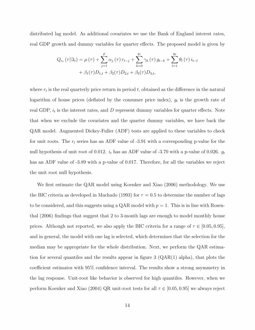
distributed lag model. As additional covariates we use the Bank of England interest rates,
real GDP growth and dummy variables for quarter effects. The proposed model is given by
Qrt(τ |ℑt) = µ (τ) +
p∑
j=1
αj (τ) rt−j +
q1∑
k=0
γk (τ) gt−k +
q2∑
l=1
θl (τ) it−l
+ β1(τ)D1,t + β2(τ)D2,t + β3(τ)D3,t,
where rt is the real quarterly price return in period t, obtained as the difference in the natural
logarithm of house prices (deflated by the consumer price index), gt is the growth rate of
real GDP, it is the interest rates, and D represent dummy variables for quarter effects. Note
that when we exclude the covariates and the quarter dummy variables, we have back the
QAR model. Augmented Dickey-Fuller (ADF) tests are applied to these variables to check
for unit roots. The rt series has an ADF value of -3.91 with a corresponding p-value for the
null hypothesis of unit root of 0.012. it has an ADF value of -3.70 with a p-value of 0.026. gt
has an ADF value of -3.89 with a p-value of 0.017. Therefore, for all the variables we reject
the unit root null hypothesis.
We first estimate the QAR model using Koenker and Xiao (2006) methodology. We use
the BIC criteria as developed in Machado (1993) for τ = 0.5 to determine the number of lags
to be considered, and this suggests using a QAR model with p = 1. This is in line with Rosen-
thal (2006) findings that suggest that 2 to 3-month lags are enough to model monthly house
prices. Although not reported, we also apply the BIC criteria for a range of τ ∈ [0.05, 0.95],
and in general, the model with one lag is selected, which determines that the selection for the
median may be appropriate for the whole distribution. Next, we perform the QAR estima-
tion for several quantiles and the results appear in figure 3 (QAR(1) alpha), that plots the
coefficient estimates with 95% confidence interval. The results show a strong asymmetry in
the lag response. Unit-root like behavior is observed for high quantiles. However, when we
perform Koenker and Xiao (2004) QR unit-root tests for all τ ∈ [0.05, 0.95] we always reject
14
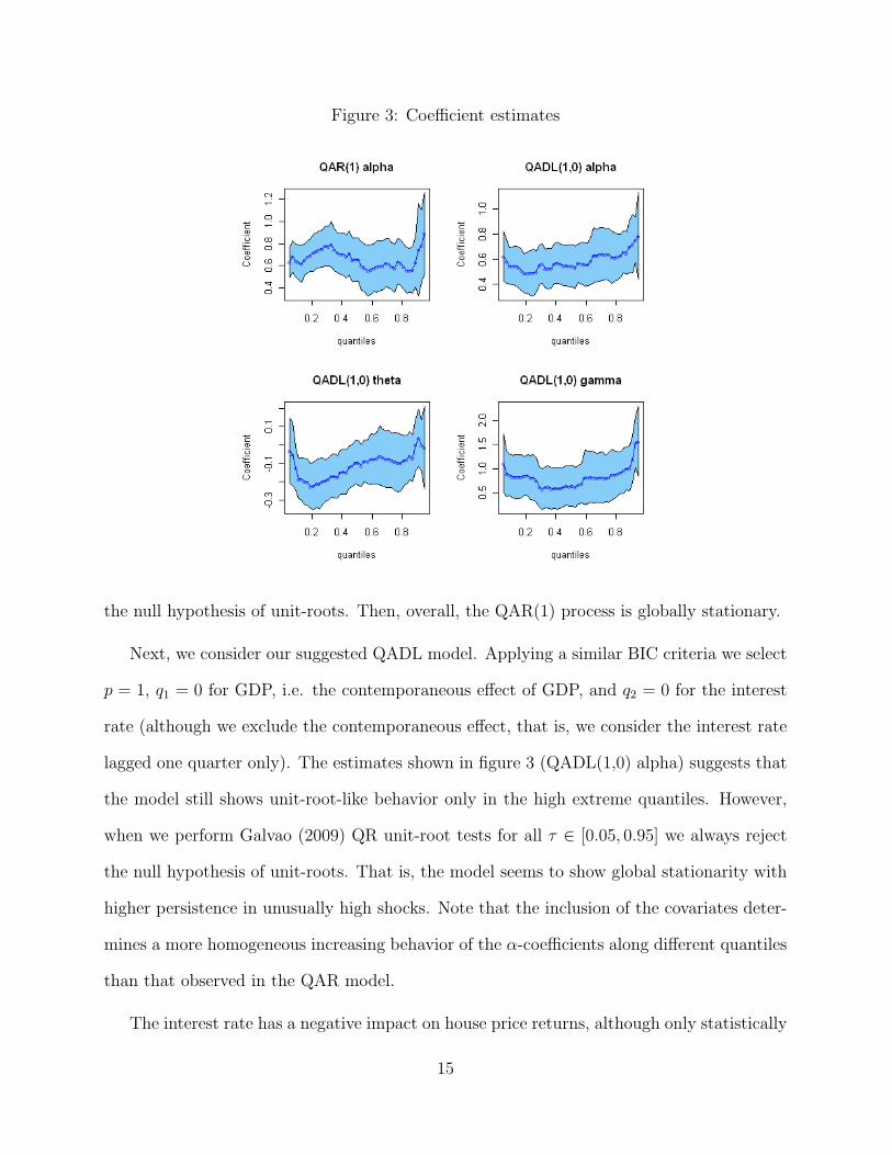
Figure 3: Coefficient estimates
the null hypothesis of unit-roots. Then, overall, the QAR(1) process is globally stationary.
Next, we consider our suggested QADL model. Applying a similar BIC criteria we select
p = 1, q1 = 0 for GDP, i.e. the contemporaneous effect of GDP, and q2 = 0 for the interest
rate (although we exclude the contemporaneous effect, that is, we consider the interest rate
lagged one quarter only). The estimates shown in figure 3 (QADL(1,0) alpha) suggests that
the model still shows unit-root-like behavior only in the high extreme quantiles. However,
when we perform Galvao (2009) QR unit-root tests for all τ ∈ [0.05, 0.95] we always reject
the null hypothesis of unit-roots. That is, the model seems to show global stationarity with
higher persistence in unusually high shocks. Note that the inclusion of the covariates deter-
mines a more homogeneous increasing behavior of the α-coefficients along different quantiles
than that observed in the QAR model.
The interest rate has a negative impact on house price returns, although only statistically
15

significant for low quantiles (see figure 3, QADL(1,0) theta). In other words, this variable
may have an effect to prevent busts, but it may not deter house price booms. Therefore, the
policy followed by the Bank of England of cutting the interest rate to prevent a house price
collapse may have the desired effect. A Kolmogorov-Smirnov test of the hypothesis that
supτ∈T θ1 (τ) = 0 gives a KS value of 12.8. Looking at Andrews (1993, p.840) the critical
values are 8.19, 9.84, 13.01 for 10%, 5% and 1% significance levels respectively. Therefore,
the interest rate has an effect different from zero at the 5% significance level.
Real GDP growth has a larger impact on low and high quantiles than for medium quan-
tiles (see figure 3, QADL(1,0) gamma). For low quantiles, this is interpreted as the fact
that GDP growth reactivates the housing market when returns are low, while it might be
contributing to house prices’ busts (as that in the early 1990’s). Moreover, it contributes
to sustaining house prices increments. In other words, periods of unusually conditional high
returns are very responsive to GDP growth. Note that the estimated coefficient for very
high quantiles is greater than 1, although not statistically different from this value except
for a few quantiles. Poterba (1991) and Capozza et al. (2002) among others, provide evi-
dence on the asymmetric responses of house prices to income shocks. The QADL estimates
present this feature of house prices to income shocks, but restricted to high quantiles. A
Kolmogorov-Smirnov test of the hypothesis that supτ∈T γ0 (τ) = 0 gives a KS value of 33.1,
which by the critical values discussed above show that the effect of GDP is not zero (as
expected from the figure). However, the hypothesis that supτ∈T γ0 (τ) = 1 gives KS=4.1.
Then, overall, the effect of GDP growth on house price returns is not different from 1.
In summary, the application illustrates the usefulness of the QADL process to model
asymmetric behavior in time series. Of particular importance are the asymmetries in the
slope of the lagged dependent variable and other covariates in both extreme low and high
quantiles. In this case, the conditional mean may be a misleading estimator in periods of
16
extremely low and high conditional returns, which are those when policymakers are keener
to intervene or to predict future behavior.
V. Conclusion
We have developed a quantile autoregression distributed lag model (QADL). Quantile re-
gression methods provide a framework for robust estimation and inference and allow one to
explore a variety of forms of conditional heterogeneity under less compelling distributional
assumptions. The proposed model is able to accommodate exogenous covariates in the QAR
model. Monte Carlo simulations are conducted to evaluate the finite sample performance
of the QADL estimator. It is shown that the simple quantile autoregression estimator is
severely biased by omitting exogenous variables, while the QADL is generally unbiased. In
addition, the QADL approach outperforms the ordinary augmented distributed lag approach
in terms of root mean square error for non-Gaussian heavy tail distributions.
We illustrate the QADL model with an application to quarterly house price returns data
in the UK. The results show that house price returns have an asymmetric autoregressive
behavior, and that real GDP growth and interest rates have an asymmetric impact on house
prices variations along the quantiles. In addition, the results suggest that unit root behav-
ior is present only in the high extreme quantiles. Thus, the model seems to show global
stationarity with some persistence in unusually high returns. The inclusion of covariates
determines a more homogeneous increasing behavior of the autoregressive coefficients along
different quantiles than that observed in the QAR model, but maintains the persistence in
the high quantiles. The interest rate has a negative impact on house prices, mostly significant
for low quantiles. This can be interpreted as the fact that the interest rates have an effect on
stimulating the demand in the real estate market when returns are low, but it does not deter
house prices booms. In addition, there is evidence that the impact of GDP on house prices
17

presents an asymmetric persistence and it is stronger for low and high quantiles. For low
quantiles, this is interpreted as the fact that GDP growth reactivates the real estate market
when returns are low, while it might be contributing to house prices’ busts. Moreover, it
contributes to sustaining house prices booms. In other words, periods of unusually high
returns are very responsive to GDP growth.
References
Andrews, D. W. K. (1993). Tests for parameter instability and structural change with
unknown change point. Econometrica 61, 821–856.
Banks, J. and S. Tanner (2002). Household portfolios in the united kingdom. In L. Guiso,
M. Haliassos, and T. Japelli (Eds.), Household Portfolios, Chapter 6. Cambridge: MIT
Press.
Beaudry, P. and G. Koop (1993). Do recessions permanently change output? Journal of
Monetary Economics 31, 149–163.
Bofinger, E. (1975). Estimation of a density function using order statistics. Australian
Journal of Statistics 17, 1–7.
Campbell, J. and J. Cocco (2007). How do house prices affect consumption? evidence from
micro data. Journal of Monetary Economics 54, 591–621.
Capozza, D. R., P. H. Hendershott, C. Mack, and C. J. Mayer (2002). Determinants of real
house price dynamics. NBER Working Paper Series 9262.
Engle, R. F. and S. Manganelli (2004). Caviar: Conditional autoregressive value at risk by
regression quantiles. Journal of Business and Economic Statistics 22, 367–381.
Galvao, A. F. (2009). Unit root quantile autoregression testing using covariates. Journal of
Econometrics 152, 165–178.
Galvao, A. F., G. Montes-Rojas, and S. Y. Park (2009). Quantile autoregressive distributed
lag model with an application to house price returns. City University London, Department
of Economics Discussion Paper Series 09/04.
18

Gourieroux, C. and J. Jasiak (2008). Dynamic quantile models. Journal of Econometrics 147,
198–205.
Koenker, R. (2005). Quantile Regression. New York, New York: Cambridge University
Press.
Koenker, R. and G. W. Bassett (1978). Regression quantiles. Econometrica 46, 33–49.
Koenker, R. and Z. Xiao (2004). Unit root quantile autoregression inference. Journal of the
American Statistical Association 99, 775–787.
Koenker, R. and Z. Xiao (2006). Quantile autoregression. Journal of the American Statistical
Association 101, 980–990.
Machado, J. A. F. (1993). Robust model selection and m-estimation. Econometric Theory 9,
478–493.
Mankiew, N. G. and D. N. Weil (1989). The baby boom, the baby bust, and the housing
market. Regional Science and Urban Economics 19, 235–258.
Muellbauer, J. and A. Murphy (1997). Booms and busts in the uk housing market. The
Economic Journal 107, 1701–1727.
Neocleous, T. and S. Portnoy (2008). On monotonicity of regression quantile functions.
Statistics and Probability Letters In Press, http://eprints.gla.ac.uk/3799/.
Ortalo-Magne, F. and S. Rady (1999). Boom in, bust out: Young households and the housing
price cycle. European Economic Review 43, 755–766.
Ortalo-Magne, F. and S. Rady (2006). Housing market dynamics: On the contribution of
income shocks and credit constraints. Review of Economic Studies 73, 459–485.
Poterba, J. (1991). House price dynamics: The role of tax policy and demography. Brookings
Papers on Economic Activity 2, 143–203.
Powell, J. L. (1986). Censored regression quantiles. Journal of Econometrics 32, 143–155.
Rosenthal, L. (2006). Efficiency and seasonality in the uk housing market, 1991-2001. Oxford
Bulletin of Economics and Statistics 68, 289–317.
19

Xiao, Z. (2009). Quantile cointegrating regression. Journal of Econometrics 150, 248–260.
Xiao, Z. and R. Koenker (2009). Conditional quantile estimation for generalized autoregres-
sive conditional heteroscedasticity models. Journal of the American Statistical Associa-
tion 104(488), 1696–1712.
20