City, University of London Institutional Repository

Citation: Haslip, G. G. & Kaishev, V. K. (2015). A Novel Fourier Transform B-spline Method for Option Pricing. Journal of Computational Finance, 19(1), pp. 41-74.

This is the accepted version of the paper.

This version of the publication may differ from the final published version.

Permanent repository link: http://openaccess.city.ac.uk/11985/

Link to published version:

Copyright and reuse: City Research Online aims to make research outputs of City, University of London available to a wider audience. Copyright and Moral Rights remain with the author(s) and/or copyright holders. URLs from City Research Online may be freely distributed and linked to.

City Research Online: http://openaccess.city.ac.uk/ publications@city.ac.uk

City Research Online

A Novel Fourier Transform B-spline Method for Option Pricing

Gareth G. Haslipa, Vladimir K. Kaisheva,∗

aCass Business School, City University London.

Abstract

We present a new efficient and robust framework for European option pricing under continuous-time asset models from the family of exponential semimartingale processes. We introduceB-spline interpolation theory to derivative pricing to provide an accurate closed-form represen-tation of the option price under an inverse Fourier transform.

We compare our method with some state-of-the-art option pricing methods, and demon-strate that it is extremely fast and accurate. This suggests a wide range of applications, includ-ing the use of more realistic asset models in high frequency trading. Examples considered inthe paper include option pricing under asset models, including stochastic volatility and jumps,computation of the Greeks, and the inverse problem of cross-sectional calibration.

Keywords: Continuous-time semimartingale models, option pricing, stochastic volatility,Fourier transform, closed-form solutions, B-splines, Peano formula, divided differencesAMS classification: 65C20, 41A15, 65R10, 65R32

∗Corresponding author contact information: Cass Business School, City University London, 106 Bunhill Row,London EC1Y 8TZ, United Kingdom. Tel.: +44 (0)20 7040 8453 Fax.: +44 (0)20 7040 8572

Email addresses: gareth@haslip.co.uk (Gareth G. Haslip), v.kaishev@city.ac.uk (VladimirK. Kaishev)

August 7, 2013

1. Introduction

Application of the Fourier transform for option pricing was pioneered by, among others, Steinand Stein (1991), and Heston (1993), who viewed the integral pricing formula as a “closed-form solution". Bakshi and Madan (2000) formalized the economic foundations for Fouriertransform based pricing and the interpretation of the characteristic function spanning the pay-off universe of all derivative instruments. Carr and Madan (1999) found that, by performingthe Fourier transform of the European option with respect to the strike price, the FFT can beused to perform the inversion. Following Carr and Madan (1999), the Fractional Fast FourierTransform (FRFT) method was developed by Chourdakis (2005). The FRFT addressed a short-coming of the FFT by providing greater resolution of option prices within the range of strikeprices being considered. Chourdakis (2005) demonstrated that the method could deliver pricesup to 45 times faster than the FFT without substantial loss of precision. Subsequently, threenew numerical methods for pricing options have emerged: (i) Integration-Along-Cut (IAC)method, described in Boyarchenko and Levendorskiı (2002) and refined in Levendorskiı andXie (2012), (ii) the Cosine (COS) method of Fang and Oosterlee (2008) that utilizes a cosine ex-pansion and Fourier transform inversion, providing fast and accurate prices across many strikeprices simultaneously, and (iii) the Convolution (CONV) method of Lord et al. (2009) thatbuilds upon the Quadrature (QUAD) method of Andricopoulos et al. (2003) and the enhancedQUAD-FFT method of O’Sullivan (2005), and provides efficient pricing across multiple strikeprices. A few variants of the FFT have also been developed, for example, the generalizedFFT of Boyarchenko and Levendorskiı (2002) and the inverse FFT (iFFT) of Boyarchenko andLevendorskiı (2008).

Alongside these developments, progress has also been made in approximation techniquesfor option pricing. Recently, Kristensen and Mele (2011) have provided a general approxima-tion framework based on Taylor series expansions of the difference between the actual optionprice under the selected asset model and that under an auxiliary pricing model for which aclosed-form solution is available. Carr and Madan (2010) provide a closed-form saddle-pointapproximation for a range of asset models and demonstrate its effectiveness for pricing deepout-of-the-money options for which the FFT method can be less effective. Indeed, as noted byBoyarchenko and Levendorskiı (2011), it should be stressed that in the context of calibration,for each maturity date, the number of strike prices is limited to about two to three dozens, andtherefore it is often quicker to invert the Fourier transform directly by numerical integrationthan to apply the FFT method.

This paper continues the pursuit of real-time option pricing and develops a practical andefficient approximation framework to address the valuation of European options under a gen-eral continuous-time asset model from the class of exponential semimartingale processes. Thisclass is rich and encompasses the majority of models utilized in finance for pricing derivatives.Examples include (i) the general families of (jump) diffusion processes such as the Black andScholes (1973) model, the Merton (1976) model and the mixed exponential model of Cai andKou (2011), (ii) pure jump Lévy processes such as the general class of linear combinationsof Gamma (LG) processes, recently introduced by Kaishev (2013), which includes as spe-cial cases, the variance gamma (VG) process introduced by Madan and Seneta (1990) and thebilateral gamma process considered by Küchler and Tappe (2008), the KoBoL model of Bo-yarchenko and Levendorskiı (2000) (a special case of which is known as the CGMY processesof Carr et al. (2002)), and the generalized hyperbolic models (see Eberlein (2001)), and (iii)affine processes, characterized by Duffie et al. (2003), which include the Heston (1993) modeland the Bates (1996) model. For properties of some of the particular examples of semimartin-

2

gale models see Eberlein et al. (2008).We will refer to our option pricing framework as the Fourier transform B-spline method

(FTBS). There are two key parts of the method. First, use of a Fourier transform based pricingintegral. Second, use of B-splines, which are very flexible piecewise polynomial functions, toapproximate integrand functions in the Fourier transform pricing integral. For the latter we usethe Lewis-Lipton representation, provided in Lewis (2001) (see also Lewis (2000)) and Lipton(2002). This method utilizes the Fourier transform to provide an option valuation formula asa contour integral in the complex plane and can be considered as a generalization of the ap-proach of Carr and Madan (1999). Formulas for option pricing in Lévy models, in the formof inverse Fourier transform integrals appeared already in Eq. (30) and (31) of Boyarchenkoand Levendorskiı (1998) (see also Boyarchenko and Levendorskiı (2000)). Several authorshave utilized the Fourier transform for option pricing. For example, Boyarchenko and Leven-dorskiı (2002) develop a numerical pricing method using a generalized FFT, and Quittard-Pinonand Randrianarivony (2010) apply this to price European options. In their more recent work,Boyarchenko and Levendorskiı (2011) develop new efficient implementations of the Fouriertransform method: (i) based on the truncation of the infinite trapezoid rule and using a novelapplication of summation by parts, (ii) a new family of pricing methods entitled the payoffmodification with Fourier transform methods (PMwFT), and (iii) conformal parabolic and hy-perbolic iFT methods, which utilize a conformal map, and yield an integral with a much betterrate of convergence. Option pricing under particular models, namely the Heston model andVG process, are considered in Levendorskiı (2012) and Innocentis (2011) respectively. Theabove methods are promising additions to the option pricing literature. We note that method(iii) above is particularly effective for accurately pricing deep out-of-the-money options, whichwe are not considering in our paper.

Bouziane (2008) utilizes the Fourier transform approach to the problem of pricing inter-est rate derivatives. In common with Carr and Madan (1999), and Chourdakis (2005), thesemethods introduce truncation error and sampling error as described by Lee (2004).

Generalizations of the Fourier pricing framework has recently been considered by Dufresneet al. (2009) and by Eberlein et al. (2010). The latter authors have shown that it is valid forthe more general class of exponential semimartingale models of the underlying asset pricedynamics.

In what follows, we utilize the extension of the Fourier transform pricing method providedby Eberlein et al. (2010), and assume the exponential semimartingale model for the asset priceevolution. Our method is based on three key ideas. First, we represent the integrand of theFourier transform pricing integral as a product of (i) a trigonometric function dependent on theoption strike price, and (ii) the semimartingale process characteristic function multiplied by aFourier transform of the option payoff with unit strike price, which is independent of the actualstrike price. Second, we interpolate the strike price independent function of part (ii) by a linearcombination of B-splines of a fixed (low) order. In this way, we express the Fourier transformpricing integral as a sum of integrals of a B-spline multiplied by the trigonometric function ofpart (i). Third, we interpret these integrals as Peano representations of divided differences ofappropriate trigonometric functions. As a result, we obtain an explicit, closed-form expressionfor the option price in the form of a linear combination of low order divided differences oftrigonometric functions, as shown in Theorem 2 of Section 3.3.3. The coefficients in this linearcombination are obtained from the spline interpolation of the strike price independent functionof part (ii). Consequently, the only strike price dependent part of our option pricing expressionare the divided differences. Therefore, the FTBS method can be used for efficient evaluation of

3

option prices not just for one fixed strike price but simultaneously for a whole set of differentstrike prices in a given range. Although the divided differences calculation is dependent onthe strike price, it does not depend on the choice of asset model and hence they can be pre-computed.

The option price evaluation under our method is very fast and accurate since the semimartin-gale process characteristic function of part (ii) above is interpolated and, hence, computed at arelatively small number of interpolation sites, and the knots of the interpolating spline are op-timally located, as described in Section 3. To our best knowledge, optimal spline interpolationtheory has not been used in the option pricing literature before. In summary, for any choice ofan exponential semimartingale model for the underlying asset price process, the option pricecalculation using our method becomes a simple procedure of (i) fitting a spline function ex-pressed as a linear combination of B-splines to a simple variant of the characteristic function,and (ii) computing a linear combination of the B-spline coefficients and the pre-computed di-vided difference factors for the choice of strike price and interest rate. As demonstrated inSection 4, this process is extremely quick and allows us to compute the option price with anyrequired accuracy.

For example, under the VG process, we can calculate European option prices across 31different strike prices accurate to five significant figures in under 20 microseconds, which im-plies a computation time of under one microsecond per option. These computation times areachieved using a modest computational environment, as described in Section 4, and do notmake use of parallel processing techniques. Our method therefore has a wide range of applica-tions in finance, ranging from pricing, marking, and hedging to calibration and high-frequencytrading.

There are several key advantages of our method over existing approximation methods foroption pricing. First, truncation error is eliminated by transforming the Fourier transform pric-ing integral to the unit interval. Second, our method is able to compute accurate option priceswith lower sampling error than other methods when using only a small number of interpolationsites. This is evidenced by our numerical examples, see Figure 1 of Section 4. Finally, thedivided difference calculation is model independent and can therefore be pre-computed andstored in a data file for future use. This enables the FTBS method to compute asset prices ex-tremely quickly at a higher level of precision than is possible using alternative approximationmethods, for most of the asset price models that we have investigated, see Figure 1 of Section4, and Tables F.6, F.7, and F.8 of Appendix F. We note that we are unaware of any similarexisting approximation methods in the option pricing literature. This is confirmed by the re-sults of the numerical comparison of our FTBS method with five other state-of-the-art optionpricing methods, namely the FFT, FRFT, IAC, COS, and CONV methods, which as we showare very competitive. In order to make this comparison computationally fair, we have diligentlyimplemented all the six option pricing methods to the best of our ability in C++ using identicalhardware.

In this paper, we illustrate the FTBS method for computing the price and sensitivities ofEuropean options but note that the method is more general and can be applied without adjust-ment to any contingent claim without early exercise or path dependent features. Additionally,the method can be adapted for pricing exotic options, as demonstrated in Haslip and Kaishev(2013) for the problem of pricing discrete lookback options.

This paper is organized as follows. The next section reviews the Fourier transform pricingframework that underlies our FTBS method. In Section 3, we introduce the application ofB-spline interpolation theory to option pricing and show how the Peano representation of a

4

divided difference with respect to a B-spline kernel is applied to provide a closed-form formulafor pricing and computing the sensitivities of European options across all strike prices. Section4 assesses the numerical performance of the FTBS method across a wide range of different assetprice models and provides detailed comparisons to the existing methods listed above. In Section5, we consider the cross-sectional calibration of the Heston model and the stochastic volatilityjump diffusion model of Bates (1996) to the implied volatility surface, and demonstrate theeffectiveness of the FTBS method relative to the FFT and FRFT methods. Section 6 concludesthe paper, and the appendices provide tables and some detailed proofs that are omitted from themain text.

2. Pricing options using the Fourier transform

In this section, we introduce the notation and assumptions of the continuous-time asset pricemodel and provide a short recap of the Fourier transform pricing framework for the valuationof European options.

2.1. Notation and model assumptionsLet the stochastic process X = (Xt)t≥0 with X0 = 0 be defined on a continuous-time proba-bility space (Ω,F ,Q) with a standard complete filtration Ft, t ≥ 0. We assume that X is asemimartingale with respect to the filtration Ft, t ≥ 0, so that it satisfies X = M +A whereM = (Mt)t≥0 is a local martingale with M0 = 0 and A = (At)t≥0 is a bounded variation pro-cess with A0 = 0. Let St ≥ 0 denote the price at time t > 0 of an asset whose price dynamicsfollows an exponential semimartingale process given by

St = S0e(r−q)t+Xt , (1)

where r is the risk-free interest rate, and q is the continuous income yield provided by the as-set. In Eq. (1), the probability measure Q is assumed to be the risk-neutral measure under theassumption of no arbitrage, where e−rtSt is a martingale. For further properties of semimartin-gales we refer to Jacod and Shiryaev (2003).

2.2. The Fourier transformThe FTBS method is built on the foundations of the Fourier transform. We now introducethis Fourier pricing method and develop a pricing formula for European options. In Section 3,the pricing formula is approximated using an optimal spline interpolation, which provides fastconvergence to the true price.

The Fourier transform method provides a direct integration formula for option prices undera range of payoffs, independent of the choice of an asset model.

Proposition 1 (European call option pricing formula). If MXT(v) exists for all v ∈ (1, α)

with α > 1, then the European call option price, C(T,K), is given by

C(T,K) = −Ke−rT

2π

iv+∞∫iv−∞

e−izkφXT(−z)

dz

z2 − iz, (2)

where MXT(v) =

∞∫−∞

evxfXT(x)dx, and

k = log(S0

K) + (r − q)T. (3)

5

PROOF. The proof is straightforward and can be found e.g. in Eberlein et al. (2010) (seeExample 5.1 therein).

The pricing formula in Eq. (2) is an interesting direct integration formula for the Europeancall option, but in this form it exhibits a number of difficulties. First, the choice of contour inte-gration parameter, v, is important and has a significant impact on the behavior of the integrandand, hence, the convergence properties of the formula. Lord and Kahl (2007) investigate thechoice of v in depth and provide optimal choice for particular asset models when pricing Eu-ropean options. For a more recent investigation of the optimal choice of parameter of contourintegration see Section 2.7 of Boyarchenko and Levendorskiı (2011). Second, the integrationmust be performed over an infinite interval, and care must be taken to avoid truncation error.

In our presentation of the FTBS method, we prefer to utilize an alternative form of Eq. (2)provided by Lewis (2001) and Lipton (2002).

Proposition 2 (Alternative European call option pricing formula). If MXT(v) exists for all

v ∈ (α, β) with α < 12

and β > 1, then the European call option price, C(T,K), is given by

C(T,K) = S0e−qT −

√S0Ke

−(r+q)T2

π

∫ ∞0

Re[eiukφXT

(u− i

2

)]du

u2 + 14

, (4)

where k is given by Eq. (3).

Remark 1. The pricing formula in Eq. (4) can be considered a compromise (for the purposeof ease of use) to Eq. (2), where instead of identifying the optimal choice of the contourparameter for a particular asset price model, it is fixed at a level that generally performs wellacross a range of models. In developing the FTBS method we have considered different contourparameters, and we note that the method is applicable for choices different than v = 0.5.However, for simplicity of the presentation, and ease of use of the method in deriving Theorem2 of Section 3.3.3, we have chosen to use the above alternative form with v = 0.5, which worksreasonably well for a wide choice of models and parameters.

We refer the reader to Theorem 4 in Appendix C, which is a version of Theorem 2 that isapplicable in the general case v > 1, and note that this can easily be extended to the casev < 0. We note that the simplified pricing formula Eq. (4) still exhibits the difficulty with thetruncation error of the upper limit of integration, which we address in the next section.

3. The Fourier Transform B-spline pricing method

In this section, we provide a full derivation of the FTBS method in the context of pricing Eu-ropean call options on an underlying asset. In addition, we consider the problem of calculatingthe Greeks and apply the FTBS method to compute the sensitivities of European call options.However, as noted in the introduction, the method is more general and can be applied to a widerrange of options by modifying the payoff function in the pricing formula.

3.1. Simplification of the pricing formulaWe now present an alternative representation of the pricing formula in Eq. (4) in which the inte-grand is decomposed into the product of (i) a trigonometric function dependent on the option’sstrike price, and (ii) the real and imaginary parts of the semimartingale process characteristicfunction multiplied by the Fourier transform of the option payoff with unit strike, which isindependent of the actual strike price.

6

Theorem 1 (Strike-separable pricing formula). If MXT(v) exists for all v ∈ (α, β) with

α < 12

and β > 1, then the European call option price C(T,K) is given by

C(T,K) = S0e−qT − 1

π

√S0Ke

−(r+q)T2 I(k), (5)

where

I(k) =

1∫0

cos(

1−ttk)s1(t)dt+

1∫0

sin(

1−ttk)s2(t)dt, (6)

s1(t) =Re[φXT

(1−tt− i

2)]

1− 2t+ 54t2

, s2(t) = −Im[φXT

(1−tt− i

2)]

1− 2t+ 54t2

, (7)

and k is defined in Eq. (3).

PROOF. Using the Euler identity, one can expand eiuk in Eq. (4) as cosuk + i sinuk. We thenexpress φXt(u− i

2) in terms of its real and imaginary parts. Multiplying together and discarding

imaginary terms yields the following simplification for the integral in Eq. (4)∫ ∞0

Re[φXt(u− i

2)]

cosuk − Im[φXt(u− i

2)]

sinuk

u2 + 14

du,

which we denote by I(k). We then make the change of variable u = 1−tt

. Noting that the limitsu = 0 and u = ∞ correspond to t = 1 and t = 0, respectively, and du = − 1

t2dt, the integral

becomes

I(k) =

∫ 1

0

Re[φXt(

1−tt− i

2)]

cos(

1−ttk)− Im

[φXt(

1−tt− i

2)]

sin(

1−ttk)

t2[(

1−tt

)2+ 1

4

] dt.

Finally, by simplifying the denominator and defining s1(t) and s2(t) as above, the result fol-lows.

Remark 2. We make two important observations about strike-separable pricing formula in Eq.(5). First, integration is now performed over the unit interval. Specifically, we have appliedthe change of variables u = 1−t

twhich transforms the upper limit of integration from infinity

to zero, and the lower limits of integration from zero to one. Thus, integration is performedover the unit interval [0, 1]. In this way we eliminate the truncation error which comes from thenecessity to truncate the limit at infinity in the original expression of Eq. (4). This means thatit is no longer necessary to carefully identify a truncation point for each asset price model byconsidering how quickly the characteristic function decays to zero. Second, we have separatedthe integrand into the product of cos

(1−ttk)

or sin(

1−ttk), which are dependent on the strike

price, and functions s1(t) and s2(t), which are independent of the strike price. This innovationis one of the foundations of the FTBS method since it allows us to price options at differentstrike prices in an extremely efficient manner.

The above remark highlights a significant improvement to many of the existing numerical meth-ods of option pricing based on the Fourier transform, most of which require careful examinationof the characteristic function to minimize the truncation error in the resulting option price.

7

3.2. The GreeksPricing is one key aspect of the field of derivatives, another equally important aspect is hedging,which is crucial for effective risk management. We now consider the problem of computing theGreeks and demonstrate how Eq. (5) is easily extended to calculate the option price sensitivi-ties. We note that here we only consider the Greek sensitivities that are model independent andtherefore do not depend on the form of the characteristic function. For example, Vega is spe-cific to the Black-Scholes model and does not exist in the same form for a general exponentialsemimartingale process.

Corollary 1 (The Greeks). The sensitivities of the European call option price, C(T,K), tomovements in the asset price, interest rate, and the passage of time are provided by ∆C(T,K) =∂C(T,K)∂S0

and ΓC(T,K) = ∂2C(T,K)

∂S20

with respect to the asset price, PC(T,K) = ∂C(T,K)∂r

with

respect to the interest rate, and ΘC(T,K) = ∂C(T,K)∂T

with respect to the tenor. If MXT(v)

exists for all v ∈ (α, β), with α < 12

and β > 1, then they can be computed as

∆C(T,K) = e−qT − 1

π

√KS0e−(r+q)T

2[

12I(k) + I ′(k)

](8)

ΓC(T,K) =1

S0π

√KS0e−(r+q)T

2[

14I(k)− I ′′(k)

](9)

PC(T,K) =1

π

√S0Ke

−(r+q)T2

[12I(k)− TI ′(k)

](10)

ΘC(T,K) = −qS0e−qT +

1

π

√S0Ke

−(r+q)T2

[T2I(k)− (r − q)I ′(k)

], (11)

where I ′(k) and I ′′(k) are the derivatives of the function I(k), defined in Eq. (6). These arecomputed as

I ′(k) =

1∫0

cos(

1−ttk)

∆s1(t)dt+

1∫0

sin(

1−ttk)

∆s2(t)dt (12)

I ′′(k) =

1∫0

cos(

1−ttk)

Γs1(t)dt+

1∫0

sin(

1−ttk)

Γs2(t)dt, (13)

where∆s1(t) =

1− tt

s2(t), and ∆s2(t) = −1− tt

s1(t), (14)

and

Γs1(t) =1− tt

∆s2(t) = −(1− t)2

t2s1(t),

Γs2(t) = −1− tt

∆s1(t) = −(1− t)2

t2s2(t).

PROOF. The proof of the formulae for the Greeks is provided by careful application of thechain rule when differentiating. We sketch the proof briefly for the case of ∆ and Γ and note

8

that similar logic applies in the case of P or Θ. We begin with the proof for ∆C(T,K). FromEq. (5), we have

∆C(T,K) =∂C

∂S0

= e−qT − 12π

(S0K)−12Ke

−(r+q)T2 I(k)

− 1π

√S0Ke

−(r+q)T2 I ′(k)

∂k

∂S0

. (15)

Noting that k = log(S0

K) + (r − q)T , we obtain ∂k

∂S0= 1

S0. Simplifying Eq. (15) yields the

required result.To obtain ΓC(T,K), one simply differentiates C(T,K) a second time, that is,

ΓC(T,K) = ∂∆C∂S0

, and again makes careful use of the chain rule. This yields the expression inEq. (9). Finally, to obtain the expressions for I ′(k) and I ′′(k), we differentiate Eq. (6) underthe integral sign with respect to k,

I ′(k) =d

dkI(k) =

1∫0

d

dkcos(

1−ttk)s1(t)dt+

1∫0

d

dksin(

1−ttk)s2(t)dt

= −1∫

0

sin(

1−ttk)

1−tts1(t)dt+

1∫0

cos(

1−ttk)

1−tts2(t)dt.

Defining ∆s1(t) and ∆s2(t) as in Eq. (14) provides the stated formula for I ′(k). The calcula-tion of I ′′(k) follows precisely the same logic.

We have developed simple integration formulae for pricing options and computing theirsensitivities. These form the foundations of the FTBS method and we now proceed to developclosed-form approximations to compute them. In the next section we apply spline approxima-tion theory to interpolate functions s1(t), s2(t), ∆s1(t), ∆s2(t), Γs1(t), and Γs2(t).

3.3. Developing the approximation formulaThe standard approach in option pricing for the evaluation of Eq. (5) is to apply efficient nu-merical integration techniques, such as the Gauss-Kronrod quadrature method, to calculate theintegral to the desired level of accuracy. In this section, we introduce a general approach forevaluating Eq. (5) that utilizes spline approximation theory. We have chosen to apply splinefunctions in developing our option pricing method, because they allow for the accurate approx-imation of possibly complex and oscillatory functions. For example, see Figure 7 of Kaishevet al. (2006), where B-spline basis functions are used to approximate the Doppler function,which is wildly oscillatory, especially near the origin. There are two key ideas underlying thespline approximation component of the FTBS method. First, we interpolate the functions s1(t)and s2(t) by two linear combinations of B-splines of a fixed low order.

In this way we express each of the two integrals in the expression for I(k) in Eq. (6) asa linear combination of integrals of a B-spline multiplied by cos(1−t

tk) and sin(1−t

tk), respec-

tively. Second, we interpret these integrals as Peano representations of divided differences ofappropriate trigonometric functions and obtain an explicit, closed-form expression for the op-tion price. The latter is in the form of a linear combination of low order divided differences oftrigonometric functions and is provided in Theorem 2 of Section 3.3.3. The coefficients in thislinear combination are obtained from the spline interpolation of the strike price independentfunctions s1(t) and s2(t).

9

Our method is very fast and accurate for two main reasons. First, since we extract theoscillatory components, cos

(1−ttk)

and sin(

1−ttk), from the integrand in Eq. (4), the remaining

functions, s1(t) and s2(t), are smoother and better behaved. Hence, the approximation ofthese functions requires only a relatively small number of interpolation sites at which they arecomputed and interpolated. The second reason is that, given fixed interpolation sites, the knotsof the interpolating spline are optimally located, following Gaffney and Powell (1976) andMicchelli et al. (1976). Therefore, the optimal interpolating spline provides the best possiblebound for the spline interpolation error. Moreover, it can be shown (see De Boor (2001),Chapter XII) that as the number of interpolation sites and knots increases, the error bounddecays at the rate O (|t|n ), where |t|:= maxi (ti − ti−1) is the mesh size of the sequence ofknots. In other words, the spline approximation quickly converges to the integrand functionas the number of interpolation sites, and hence knots, increases. Therefore, the FTBS methodprovides a very accurate approximation of the option price, and requires far fewer evaluationsof the approximated integrand function than using direct numerical integration. In the followingsections, we provide a brief introduction to B-splines and divided differences and formalize theideas we have described in this section to establish our main option pricing result presented inTheorem 2 of Section 3.3.3.

3.3.1. Splines, B-splines, and divided differencesIn order to derive our main result given in Theorem 2, we require some background materialon splines which we briefly introduce. Let n and l be positive integers and consider an interval[a, b] ∈ R, partitioned by the points a = tn < . . . < tn+l < tn+l+1 = b called knots. Wedefine the spline function, s(t) of order n, degree n − 1, as a piece-wise polynomial functionwhich coincides with a polynomial of degree n − 1 between the knots tn, . . . , tn+l+1. Thepolynomial pieces are smoothly joined at the knots tn+1, . . . , tn+l so that the spline is n − 2times continuously differentiable on the interval [a, b]. To introduce the set of B-spline basisfunctions, we add n − 1 additional knots at each end of the interval [a, b]. Thus, we define theextended set of knots ti2n+l

i=1 so that t1 = · · · = tn = a, a < tn+1 < · · · < tn+1 < b, andtn+l+1 = · · · = t2n+l = b.

As known by the Curry-Schoenburg theorem, polynomial splines on ti2n+li=1 form a linear

space of functions, an element, s(t), of which is represented as

s(t) =

p∑i=1

ciMi,n(t), (16)

where ci are constant coefficients, p = l + n, and Mi,n(t) are the B-spline basis functions. Thelatter are defined on ti2n+l

i=1 as the n-th order divided difference of the functionf(y) = n (max (y − t), 0)n−1 = n(y − t)n−1

+ , that is,

Mi,n(t) = Mi,n(t; ti, . . . , ti+n) = [ti, . . . , ti+n]f(y).

The n-th order (n ≥ 0) divided difference of a function f(t) is defined recurrently as

[ti, . . . , ti+n] f(t) =[ti+1, . . . , ti+n] f(t)− [ti, . . . , ti+n−1] f(t)

ti+n − ti, (17)

where [ti] f(t) = f (ti) and the points tji+nj=i are pairwise distinct. In the case when one ormore points are repeated, a derivative based formula provided in Eq. (B.1) of Appendix B.1,which appears in Ignatov and Kaishev (1989), can be used to calculate the divided difference.

10

The B-spline basis functions, Mi,n(t), i = 1, . . . , p, have some nice properties, see e.g.De Boor (2001), that will be very useful in deriving our pricing formula Eq. (22). In particular,we need the elegant Peano representation of the n-th order divided difference of a function f(x)given as

[ti, . . . , ti+n] f(x) =

∫R

Mi,n(t; ti, . . . , ti+n)f (n)(t)

n!dt, (18)

where f (n) is the n-th derivative of f . For a proof of Eq. (18) see, for example, De Boor (2001),Chapter IX.

Note that the B-spline Mi,n(t) appears as the kernel in the Peano representation given inEq. (18). This is important since in the derivation of the pricing formula in Eq. (22), weneed to evaluate integrals of the form

∫RMi,n(t; ti, . . . , ti+n)ψ(t)dt, with ψ(t) = cos

(1−ttk)

or ψ(t) = sin(

1−ttk). We shall see that it is possible to express such integrals in the form of

Eq. (18) and thus eliminate integration; replacing it with the evaluation of a simple low orderdivided difference of a function ψ(t), whose n-th derivative coincides with ψ(t). Therefore, thePeano representation plays a fundamental role in obtaining our main result, the option pricingformula given by Eq. (22) in Theorem 2.

3.3.2. Optimal B-spline interpolationIn this section, we use the spline function, s(t), defined in Eq. (16), to interpolate the integrandfunctions, s1(t) and s2(t). from the strike-separable pricing formula, given in Theorem 1. Sincethese functions are defined on the interval [0, 1], we assume that [a, b] ≡ [0, 1] in the definitionof the knot set ti2n+l

i=1 . To avoid complicating the notation, we illustrate this step only forthe function s1(t). The same reasoning and similar notation applies for s2(t). Denote the setof ν interpolation sites, which are alternatively referred to as data sites, as τ = τ1, . . . , τν,with τ1 = 0, τν = 1, and τi < τi+1, i = 1, . . . , ν. The optimal spline interpolation problemcan now be stated as follows. For the fixed set of appropriately located data sites τ , find theinterpolating function s(t), and the function C(t) that satisfy the inequality

|s1(t)− s(t)| ≤ C(t)‖s(n)1 (t)‖, (19)

where ‖f‖ = max |f(t)| : a ≤ t ≤ b and C(t) is as small as possible for all t ∈ [0, 1]. Inorder for the bound in Eq. (19) to be valid, we also assume that the functions s1(t) and s2(t)are continuous and have bounded n-th derivatives. We note that these assumptions hold for theimplemented semimartingale asset price models, as illustrated in Section 4. Furthermore, theinterpolation method developed here works even if some of these assumptions are not satisfied,in which case it may not be possible to assess the error of approximation using the bound inEq. (19).

Gaffney and Powell (1976) and Micchelli et al. (1976) independently solved the optimalinterpolation problem in Eq. (19). It turns out that the optimal interpolant, s(t), is a splinefunction of order n with exactly l = ν − n optimally located internal knots, tin+l

i=n+1, andlinear coefficients ci for i = 1, . . . , l + n. We refer to Gaffney (1978) for details of how to findthese optimal knots and coefficients. As noted by De Boor (2001), choosing the l internal knotsto be the averages of the data sites τ , that is,

tn+i =(τi+1 + . . .+ τi+n−1)

n− 1, i = 1, . . . , l, (20)

provides a very good approximation to the optimal knot set, tin+li=n+1. We have tested the

theoretically optimal knot set, implementing the subroutine SPLOPT of De Boor (2001) and11

have not found any significant improvement. We therefore recommend the averaging methodin Eq. (20) as the efficient knot selection procedure.

Another important parameter of the interpolation process is the degree n− 1 of the spline.Popular choices are quadratic, n = 3, or cubic, n = 4. We considered both choices and foundthat numerically the cubic spline does not offer additional precision over the quadratic spline,while increasing the computational complexity. There is also some evidence in approximationtheory literature, see, for example, Marsden (1974), suggesting that quadratic splines oftenprovide better fits than cubic splines. We therefore have chosen to work with quadratic splines,and in the rest of the paper we therefore use n = 3.

In summary, for given data sites τ , the choice of which is discussed in Section 3.4.1, wefollow the optimal interpolation scheme described above. We obtain quadratic spline approx-imants, s1(t) and s2(t) to s1(t) and s2(t), that are in the form of Eq. (16). The approximantss1(t) and s2(t) are defined by the sets of knots t1,i6+l1

i=1 , t2,j6+l2j=1 and coefficients c1,i, c2,j for

i = 1, . . . , p1, j = 1, . . . , p2, where p1 = l1 + 3 and p2 = l2 + 3. We note that for the com-putation of the Greeks, additional splines are used to interpolate the functions ∆s1(t), ∆s2(t),Γs1(t), and Γs2(t).

3.3.3. The Fourier transform B-spline pricing formulaIn this section, we utilize the optimal B-spline interpolation scheme presented above to developthe main result of this paper, the FTBS pricing formula. We first return to the strike-separablepricing formula in Eq. (5) of Theorem 1 and define C(T,K) to be the approximation to Eq.(5) by replacing s1(t) and s2(t) by their spline approximants s1(t) and s2(t) respectively. Thatis,

C(T,K) ≈ C(T,K) = S0e−qT −

√S0Ke

−(r+q)T2

πI(k), (21)

where

I(k) =

1∫0

cos

(1− tt

k

)s1(t)dt+

1∫0

sin

(1− tt

k

)s2(t)dt.

We note that in what follows we assume that MXT(v) exists for all v ∈ (α, β) with α < 1

2

and β > 1. To express Eq. (21) in a closed-form and eliminate integration, it suffices to (i)substitute s1(t) and s2(t) which are splines of the form given by Eq. (16), (ii) take summationin front of integration, and (iii) apply the Peano formula in Eq. (18) to each integral in thelinear combination. The latter integrals are of the form

∫RMi,n(t; ti, . . . , ti+n)ψ(t)dt, with

ψ(t) = cos(

1−ttk)

or ψ(t) = sin(

1−ttk), which are in the required form to apply the Peano

representation. Therefore, as described in Section 3.3.1, one needs to find the function ψ(t)whose n-th derivative coincides with ψ(t). Following this approach, we give our main resultstated by the following theorem, whose proof is given in Appendix B.2.

12

Theorem 2 (The Fourier Transform B-spline pricing formula).Let t1,i6+l1

i=1 , t2,j6+l2j=1 and c1,ip1

i=1, c2,jp2

j=1 be the sets of knots and linear coefficients of thequadratic spline interpolants, s1(t) and s2(t), respectively, where p1 = l1 + 3 and p2 = l2 + 3.Additionally, let k = log

(S0

K

)+ (r − q)T . The pricing formula of a European call option is

given as

C(T,K) ≈ S0e−qT − 1

π

√S0Ke

−(r+q)T2 I(k), (22)

where for k 6= 0

I(k) = 6

p1∑i=1

c1,i[t1,i, t1,i+1, t1,i+2, t1,i+3]f1(t, k)

+ 6

p2∑i=1

c2,i[t2,i, t2,i+1, t2,i+2, t2,i+3]f2(t, k), (23)

and f1 and f2 are defined as

f1(t, k) =1

12

t

(−(k2 − 2t2) cos

k(t− 1)

t− 5kt sin

k(t− 1)

t

)+ kCi

(k

t

)(−6kt cos k + (k2 − 6t2) sin k

)− k Si

(k

t

)(6kt sin k + (k2 − 6t2) cos k

)

f2(t, k) =1

12

t

(−(k2 − 2t2) cos

k(t− 1)

t− 5kt sin

k(t− 1)

t

)+ kCi

(k

t

)(6kt sin k + (k2 − 6t2) cos k

)+ k Si

(k

t

)(−6kt cos k + (k2 − 6t2) sin k

).

For k = 0, I(k) simplifies to

I(k) =

p1∑i=1

c1,i +

p2∑i=1

c2,i. (24)

Note that Ci(x) and Si(x) are the trigonometric special functions defined as

Ci(x) = −∞∫x

cos yydy and Si(x) =

x∫0

sin yydy, respectively.

PROOF. Provided in Appendix B.2

While the functions f1 and f2 in Theorem 2 may appear complicated, they can be evaluatedefficiently. Their trigonometric integrals can be computed using the Fortran library of Van-devender and Haskell (1982), which provides 17 significant figures of accuracy using seriesexpansions with pre-computed coefficients. Calculation of the divided difference is simple us-ing the standard recursive definition in Eq. (17) when the knots [ti, ti+1, ti+2, ti+3] are distinct.In the case of repeated knots, the divided differences must be calculated using the derivativebased definition in Eq. (B.1) of Appendix B.1.

13

Remark 3. We refer the reader to Theorem 4 in Appendix C, which is a version of Theorem2 that is applicable in the general case v > 1, and note that this can easily be extended to thecase v < 0. It is worth noting that the more general Theorem 4 does not lead to any additionalcomputational complexity.

The following proposition gives a bound for the absolute error of the FTBS European optionprice approximation. It shows that the FTBS method provides a fast convergence to the trueprice as the numbers, ν and l, of data sites, τ and knots, ηj,i3+l

i=3+1 increase, while the meshsizes |ηj| := maxi (ηj,i − ηj,i−1) go to zero.

Proposition 3 (FTBS Option Price Error Bound). The absolute error of the FTBS Europeanoption price, C(T,K) is bounded by∣∣∣C(T,K)− C(T,K)

∣∣∣ ≤ √S0K

πe

(r+q)T2

(C1

∥∥∥s(3)1 (t)

∥∥∥+ C2

∥∥∥s(3)2 (t)

∥∥∥) , (25)

where C1 = C1

∫ 1

0

∣∣cos(

1−ttk)∣∣ dt , C2 = C2

∫ 1

0

∣∣sin (1−ttk)∣∣ dt, Cj , j = 1, 2 are the constants

obtained from the optimal spline interpolation, sj(t) of sj(t), j = 1, 2, following Gaffney andPowell (1976), and where ‖f‖ = max |f(t)| : 0 ≤ t ≤ 1. The bound in (25) convergesto zero as the mesh sizes |ηj| := maxi (ηj,i − ηj,i−1) go to zero, at a rate O (|η|3), where η =max (|η1|, |η2|), i.e., ∣∣∣C(T,K)− C(T,K)

∣∣∣ = O(|η|3)

(26)

PROOF. Provided in Appendix B.3.

Calculation of the Greeks under the FTBS method follows the same logic as Theorem2. It uses additional B-splines to approximate functions ∆s1(t), ∆s2(t), Γs1(t), and Γs2(t).We denote the respective approximants as ∆s1(t), ∆s2(t), Γs1(t), and Γs2(t). We can thenapproximate the integrals I ′(k) and I ′′(k) from Eqs. (12) and (13) in closed-form using thePeano representation in Eq. (23).

Proposition 4 (FTBS formulae for the Greeks).Let t1,i6+l1

i=1 , t2,j6+l2j=1 and c1,ip1

i=1, c2,jp2

j=1 be the sets of knots and linear coefficients of thequadratic spline interpolants, s1(t) and s2(t), respectively, where p1 = l1 + 3 and p2 = l2 + 3.

Similarly, let the knots and linear coefficients of the quadratic spline interpolants ∆s1(t),∆s2(t), and Γs1(t), Γs2(t) be denoted by t∗1,i

6+l∗1i=1 , t∗2,j

6+l∗2j=1 and c∗1,i

p∗1i=1, c∗2,j

p∗2j=1, where

p∗1 = l∗1 + 3 and p∗2 = l∗2 + 3 for ∗ ∈ ∆,Γ.The closed-form approximations for the Greeks are obtained by replacing functions I(k),

I ′(k), and I ′′(k) in Corollary 1 by their approximants I(k), I ′(k), and I ′′(k). I(k) is definedin Theorem 2, and I ′(k) and I ′′(k) are defined as

I ′(k) = 6

p∆1∑

i=1

c∆1,i[t

∆1,i, t

∆1,i+1, t

∆1,i+2, t

∆1,i+3]f1(t, k)

+ 6

p∆2∑

i=1

c∆2,i[t

∆2,i, t

∆2,i+1, t

∆2,i+2, t

∆2,i+3]f2(t, k)

14

I ′′(k) = 6

pΓ1∑

i=1

cΓ1,i[t

Γ1,i, t

Γ1,i+1, t

Γ1,i+2, t

Γ1,i+3]f1(t, k)

+ 6

pΓ2∑

i=1

cΓ2,i[t

Γ2,i, t

Γ2,i+1, t

Γ2,i+2, t

Γ2,i+3]f2(t, k),

for k 6= 0. If k = 0, this simplifies to Eq. (C.6) in Theorem 2.

PROOF. The proof follows the same reasoning as for Theorem 2 and is therefore omitted.

3.4. Implementation of the FTBS methodThe FTBS method is straightforward to apply and, unlike other numerical methods for op-tion pricing, its implementation is largely independent of the underlying continuous-time assetmodel. The key considerations in the implementation of the FTBS method are (i) the choice ofdata sites, and (ii) the pre-computation of the divided differences [tl,i, tl,i+1, tl,i+2, tl,i+3]fl(t, k)for l = 1, 2 in Theorem 2.

It should be noted that the spline approximants, s1(t) and s2(t), are independent of the strikepriceK. Since the divided differences can be pre-computed, as we will explain in Section 3.4.2,the approximants’ strike price independence implies that the efficiency of the FTBS method forpricing many options simultaneously across a quantum of strike prices is similar to that ofpricing a single option. This is analogous to the use of the FFT of Carr and Madan (1999) forevaluating the price of European options for a range of strike prices.

3.4.1. Optimal selection of interpolation data sitesSomewhat surprisingly, the question of selecting data sites in spline interpolation has not re-ceived significant attention in the literature on approximation theory, although some consider-ations can be found in De Boor (2001). The selection of data sites depends on the smoothnessproperties of the underlying function that is to be interpolated. In areas where the function isless smooth and exhibits higher curvature, more data sites should be allocated to capture its be-havior. Intuitively, the most efficient selection of data sites should extract the most informationfrom the function with minimum number of observations. Therefore, the allocation of data sitesacross the unit interval should provide a greater weight to regions where the function exhibitsgreater curvature. We identify the data sites to sample the semimartingale process characteristicfunction by analyzing the curvature of functions s1(t) and s2(t) across a range of models andparameter choices. Our selection is based on the criteria of a compromise set τ that performsreasonably well across a large range of parameters, as opposed to being optimized for any par-ticular model. We allocate the data sites in uniform bands: 60% to [0, 0.2), 20% to [0.2, 0.6) andthe remainder to [0.6, 1]. The allocation could be improved by developing optimal data sitesallocations for specific semimartingale processes and parameter ranges. We also examine theuse of uniformly spaced data sites in the unit interval. Although uniform spacing of data sitesproduces accurate option prices, it is less efficient, since more data sites are allocated to regionsof low curvature of the functions s1(t) and s2(t) than is necessary for accurate interpolation.

3.4.2. Pre-computation of divided differencesIn computing the divided difference [tl,i, tl,i+1, tl,i+2, tl,i+3]fl(t, k) for l = 1, 2, there are twocases to consider: (i) the knots tl,i, tl,i+1, tl,i+2, tl,i+3 are all distinct, and (ii) some knots arerepeated once or more. In the former case, we can apply the recursive definition, given in Eq.

15

(17), directly, which is simple to implement computationally. In the case of repeated knots, thederivative definition, given in Eq. (B.1) of Appendix B.1, of a divided difference should beapplied.

In our case, we have to evaluate the divided differences at the following repeated knots:[0, 0, 0, tl,4]fl, [0, 0, tl,4, tl,5]fl, [tl,k+3, tl,k+4, 1, 1]fl, and [tl,k+4, 1, 1, 1]fl for l = 1, 2. Althoughalgebraically involved, these are easily explicitly expressed with the aid of symbolic algebraicsoftware, such as Mathematica, as shown in Appendix B.4. Note that, since the divided differ-ences at repeated knots are evaluated just a single time at the endpoints, their complicated formdoes not have an impact on the time it takes to compute the option price.

Returning to the FTBS pricing formula in Theorem 2, we make an important observation.The divided differences of functions f1(t, k) and f2(t, k) across the knots t1,i6+l1

i=1 ,t2,i6+l2

i=1 depend only on the choice of knots and k. They are independent of the choice of theexponential semimartingale process. Therefore, for a fixed set of data sites and correspondingoptimal knots, we can pre-compute the divided differences for different values of k and do notneed to calculate this each time an option is priced for a different value of k. Furthermore, if weuse the same data sites and knots for the Greeks, then the pre-computed divided differences canbe applied for both pricing and computing the option price sensitivities. In all our numericalexamples provided in Section 4, we pre-compute the divided differences using the allocationof data sites described in Section 3.4.1. We find that this choice of data sites provides veryaccurate results across the wide range of models considered.

The pre-computation of divided differences is a significant advantage of the FTBS method,since pricing options becomes a simple procedure of fitting the functions s1(t) and s2(t) usingB-spline interpolation, and then computing the sum in Eq. (23) of products of the B-splinecoefficients and the pre-computed divided differences. The divided differences can be pre-computed in two ways, depending on the option pricing application. First, for the purposesof calibration, one would need to compute the divided differences for a fixed set of values ofk. This set is determined by the relevant strike prices and maturity times, the interest rate,and the dividend rate, at the calibration date (see Eq. (3)). Therefore, at the beginning ofthe calibration process, the divided differences can be pre-computed exactly for all requiredvalues of k. This is a very fast process that takes approximately one to two milliseconds, andis negligible relative to the overall calibration time (see Table 1 of Section 5, where calibrationtimes are measured in the order of seconds). Second, in the case of real-time applications, suchas high frequency trading, it may be necessary to compute option prices for values of k that arerapidly changing. For example, as time elapses, the share price will move, and maturities willshorten. In this case, it is necessary to pre-compute the divided differences at a fine resolutionof possible values of k.

We now describe an algorithm to implement the pre-computation of the divided differencesin this second case. Let kmin and kmax denote the minimum and maximum moneyness of theoptions being considered, where we define the moneyness of an option as k = log

(S0

K

)+ (r−

q)T . For example, if we consider the range for log(S0

k) to be [−1, 2], r − q to be [0%, 10%],

and T to be [0, 10], then the possible range for k could be assumed to be [kmin, kmax], wherekmin = −1 and kmax = 3. Note that this covers the full market of typically traded call options.For example, if S0 = 100, then strike prices could range from K = 15 to 270 over any choiceof r − q ∈ [0%, 10%] and T ∈ [0, 10]. We denote the divided differences as

DvD1i (k) = [t1,i, t1,i+1, t1,i+2, t1,i+3 ]f1(t, k)

DvD2j (k) = [t2,i, t2,j+1, t2,j+2, t2,j+3]f2(t, k),

16

where i = 1, . . . , p1 and j = 1, . . . , p2.To approximate DvD1

i (k) and DvD2j (k) for a given k ∈ [kmin, kmax], we divide the in-

terval [kmin, kmax] uniformly using N evenly spaced points with width δ = kmax−kminN−1

. The ex-pressions DvD1

i (km) and DvD2j (km) containing the divided differences should therefore be

pre-computed for i = 1, . . . , p1, j = 1, . . . , p2, andm = 1, . . . , N , where km = kmin+(m−1)δ.Thanks to modern computing power, the values of DvD1

i (km) and DvD2j (km) across per-

missible values of i, j, and m can comfortably be held in RAM at a very fine resolution. Thisreduces the need for interpolation in the case where km < k < km+1 for some m ∈ 1, . . . , N .For example, if N is chosen such that the spacing δ = km − km−1 between neighboring km isδ = 1E-5, then, for p1 = p2 = p = 100 knots, kmin = −1 and kmax = 3, the total memoryrequired to store all values of the pre-computed divided differences is under one gigabyte. Thisis well within the capability of standard computing systems. In such an implementation, it isreasonable to choose the nearest km to the specified k, hence, avoiding the need for interpola-tion.

Since the B-spline interpolation of s1(t) and s2(t) can be performed very quickly and withgood precision, the FTBS method is able to compute precise option prices in a very efficientmanner. Moreover, once the divided differences have been pre-computed and the B-splineshave been fitted, computing the price of options for different strike prices requires only calcu-

lating S0e−qT − 1

π

√S0Ke

−(r+q)2 and performing p1 +p2 multiplication and addition operations,

as can be seen from Eqs. (22) and (23). Since typically only 50 to 100 data sites are required,this computation is extremely fast.

If a coarser partition of [kmin, kmax] is employed to approximate k, then simple linear in-terpolation can be applied to compute the required vector of divided difference between theneighboring values of kj . This adds only a slight overhead to the calculation, requiring an ex-tra p multiplication, p division, and 4p addition operations, as is evident from examining theformula for linear interpolation.

Finally, we note that in the implementation, the divided differences should be stored incontiguous memory in a simple array, since the appropriate memory offset for specified indicesi, j, and m can be computed directly. This ensures that the divided difference array for valuingan option can be accessed instantly.

3.4.3. Recommended configuration and algorithm implementing the FTBS methodIn our implementation of the FTBS method we have used identical sets of data sites and knotsfor the quadratic spline interpolants, s1(t) and s2(t) to minimize the number of evaluations ofthe asset price process characteristic function. In Algorithm 1 and Algorithm 2, we provide asimple implementation of the FTBS method, which is applied in Section 4 for all the numericalexamples. In order to provide practical recommendations for the configuration of the FTBSmethod, in Table F.3 of Appendix F we provide prescriptions for choosing the number of datasites required to achieve a desired level of precision, for all the asset price models consideredin the paper.

4. Numerical evaluation of the FTBS method

As described in Section 1, a variety of different methods for pricing European options havebeen developed in recent years. In order to assess the effectiveness of the FTBS method, wecompare it to the key state-of-the-art methods in the literature, to both verify its accuracy inpricing European options, and provide a guide to the relative speeds of the different methods.

17

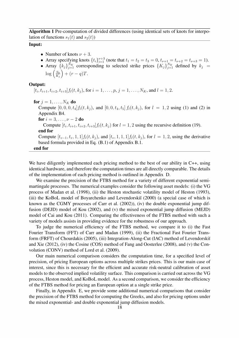
Algorithm 1 Pre-computation of divided differences (using identical sets of knots for interpo-lation of functions s1(t) and s2(t))Input:

• Number of knots ν + 3.• Array specifying knots tiν+3

i=1 (note that t1 = t2 = t3 = 0, tν+1 = tν+2 = tν+3 = 1).• Array kjNK

j=1 corresponding to selected strike prices KjNKj=1 defined by kj =

log(S0

Kj

)+ (r − q)T .

Output:[ti, ti+1, ti+2, ti+3]fl(t, kj), for i = 1, . . . , p, j = 1, . . . , NK , and l = 1, 2.

for j = 1, . . . , NK doCompute [0, 0, 0, t4]fl(t, kj), and [0, 0, t4, t5] fl(t, kj), for l = 1, 2 using (1) and (2) inAppendix B4.for i = 3, . . . , ν − 2 do

Compute [ti, ti+1, ti+2, ti+3]fl(t, kj) for l = 1, 2 using the recursive definition (19).end forCompute [tv−1, tv, 1, 1]fl(t, kj), and [tv, 1, 1, 1]fl(t, kj), for l = 1, 2, using the derivativebased formula provided in Eq. (B.1) of Appendix B.1.

end for

We have diligently implemented each pricing method to the best of our ability in C++, usingidentical hardware, and therefore the computation times are all directly comparable. The detailsof the implementation of each pricing method is outlined in Appendix D.

We examine the precision of the FTBS method for a variety of different exponential semi-martingale processes. The numerical examples consider the following asset models: (i) the VGprocess of Madan et al. (1998), (ii) the Heston stochastic volatility model of Heston (1993),(iii) the KoBoL model of Boyarchenko and Levendorskiı (2000) (a special case of which isknown as the CGMY processes of Carr et al. (2002)), (iv) the double exponential jump dif-fusion (DEJD) model of Kou (2002), and (v) the mixed exponential jump diffusion (MEJD)model of Cai and Kou (2011). Comparing the effectiveness of the FTBS method with such avariety of models assists in providing evidence for the robustness of our approach.

To judge the numerical efficiency of the FTBS method, we compare it to (i) the FastFourier Transform (FFT) of Carr and Madan (1999), (ii) the Fractional Fast Fourier Trans-form (FRFT) of Chourdakis (2005), (iii) Integration-Along-Cut (IAC) method of Levendorskiıand Xie (2012), (iv) the Cosine (COS) method of Fang and Oosterlee (2008), and (v) the Con-volution (CONV) method of Lord et al. (2009).

Our main numerical comparison considers the computation time, for a specified level ofprecision, of pricing European options across multiple strikes prices. This is our main case ofinterest, since this is necessary for the efficient and accurate risk-neutral calibration of assetmodels to the observed implied volatility surface. This comparison is carried out across the VGprocess, Heston model, and KoBoL model. As a second comparison, we consider the efficiencyof the FTBS method for pricing an European option at a single strike price.

Finally, in Appendix E, we provide some additional numerical comparisons that considerthe precision of the FTBS method for computing the Greeks, and also for pricing options underthe mixed exponential- and double exponential jump diffusion models.

18

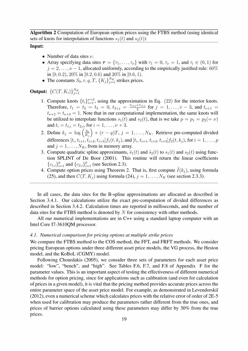
Algorithm 2 Computation of European option prices using the FTBS method (using identicalsets of knots for interpolation of functions s1(t) and s2(t))Input:

• Number of data sites ν.• Array specifying data sites τ = τ1, . . . , τν with τ1 = 0, τν = 1, and τi ∈ (0, 1) forj = 2, . . . , ν − 1, allocated uniformly, according to the empirically justified rule: 60%in [0, 0.2), 20% in [0.2, 0.6) and 20% in [0.6, 1).• The constants S0, r, q, T , KjNK

j=1 strikes prices.

Output: C(T,Ki)NKj=1

1. Compute knots tiν+3i=1 , using the approximation in Eq. (22) for the interior knots.

Therefore, t1 = t2 = t3 = 0, t3+j =τi+j+τi+j

2for j = 1, . . . , v − 3, and tν+1 =

tν+2 = tν+3 = 1. Note that in our computational implementation, the same knots willbe utilized to interpolate functions s1(t) and s2(t), that is we take p = p1 = p2(= ν)and ti = t1,i = t2,i, for i = 1, . . . , ν + 3.

2. Define kj = log(S0

Kj

)+ (r − q)T , j = 1, . . . , NK . Retrieve pre-computed divided

differences [ti, ti+1, ti+2, ti+3]f1(t, kj), and [ti, ti+1, ti+2, ti+3]f2(t, kj), for i = 1, . . . , pand j = 1, . . . , NK , from in memory array.

3. Compute quadratic spline approximants, s1(t) and s2(t) to s1(t) and s2(t) using func-tion SPLINT of De Boor (2001). This routine will return the linear coefficientsc1,ipi=1 and c2,ipi=1 (see Section 2.3).

4. Compute option prices using Theorem 2. That is, first compute I(kj), using formula(25), and then C(T,Kj) using formula (24), j = 1, . . . , NK (see section 2.3.3).

In all cases, the data sites for the B-spline approximations are allocated as described inSection 3.4.1. Our calculations utilize the exact pre-computation of divided differences asdescribed in Section 3.4.2. Calculation times are reported in milliseconds, and the number ofdata sites for the FTBS method is denoted by N for consistency with other methods.

All our numerical implementations are in C++ using a standard laptop computer with anIntel Core I7-3610QM processor.

4.1. Numerical comparison for pricing options at multiple strike pricesWe compare the FTBS method to the COS method, the FFT, and FRFT methods. We considerpricing European options under three different asset price models, the VG process, the Hestonmodel, and the KoBoL (CGMY) model.

Following Chourdakis (2005), we consider three sets of parameters for each asset pricemodel: “low”, “bench”, and “high”. See Tables F.6, F.7, and F.8 of Appendix F for theparameter values. This is an important aspect of testing the effectiveness of different numericalmethods for option pricing, since for applications such as calibration (and even for calculationof prices in a given model), it is vital that the pricing method provides accurate prices across theentire parameter space of the asset price model. For example, as demonstrated in Levendorskiı(2012), even a numerical scheme which calculates prices with the relative error of order of 2E-5when used for calibration may produce the parameters rather different from the true ones, andprices of barrier options calculated using these parameters may differ by 30% from the trueprices.

19

In the case of the VG process, and Heston model, these parameter sets are taken directlyfrom Chourdakis (2005), and in the case of the KoBoL (CGMY) model, we have utilizedparameters that represent low, medium, and high levels of volatility (based on densities a, b,and e, from Figure 1 of Carr et al. (2002)) and have used the same maturities as Chourdakis(2005).

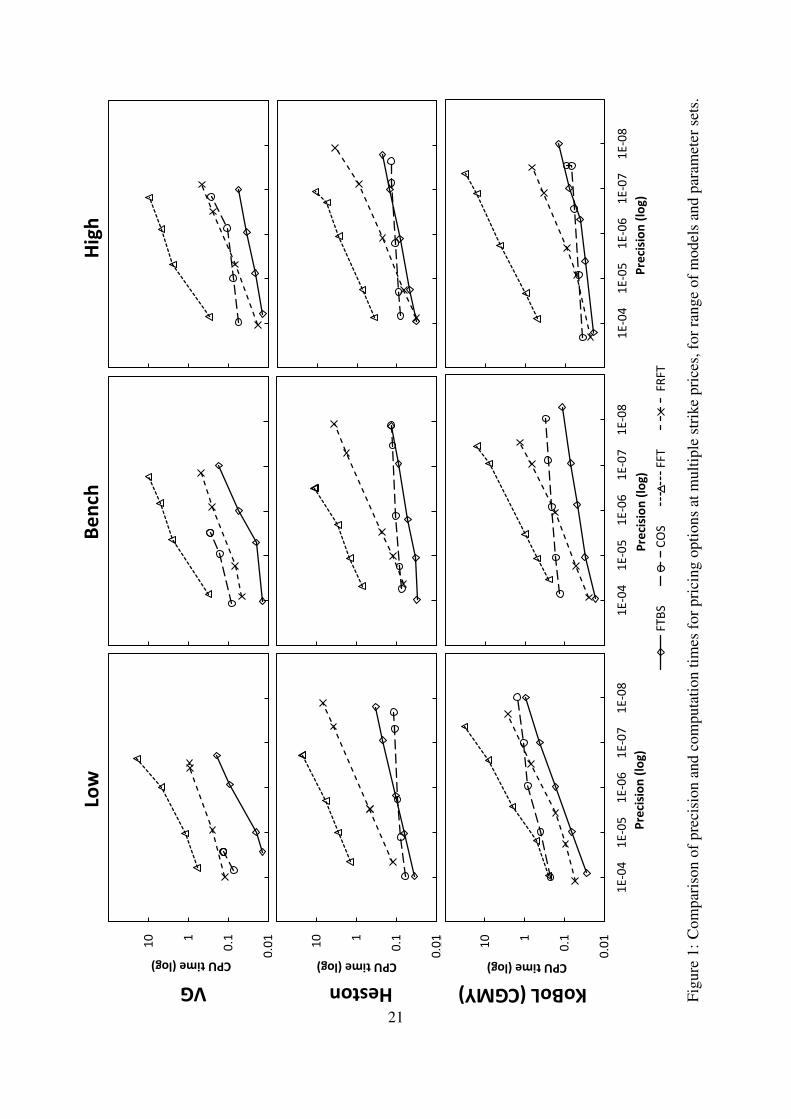
In Figure 1, we provide a graphical comparison of the FTBS method to the above pricingmethods, and across the above asset price models. Specifically, we compare the calculationtime to the level of precision for pricing European options across 31 strike prices in a singlecomputation, where the axes are in logarithmic scale. The precision level is defined as themaximum absolute error across the 31 computed option prices. Note that for the multiple strikecomparison, we computed the reference option price values using integration in Mathematicato compute the inverse Fourier integral with very high numerical precision, and verified thecorrectness of the reference prices by applying each option pricing method at its highest levelof accuracy (by setting N to a large integer).

The computation times and precision levels underlying the graphs in Figure 1 are providedin Tables F.6, F.7, and F.8, of Appendix F, where we provide several measures of precision.Namely, we give (i) the absolute error, which is the maximum absolute error, (ii) mean error,which is the average absolute error, and (iii) RMSE, which is the root mean square error.

The numerical examples provide evidence that for the problem of pricing European optionsacross multiple strike prices, the FTBS method achieves excellent efficiency, that is, a com-bination of accuracy and speed, across the different exponential semimartingale models andnumerical pricing methods considered. In particular, for the VG process, the FTBS methoddominates the other three option pricing methods at all precision levels considered from 1E-4to 1E-71.

For the Heston model, the FTBS method dominates all other comparison pricing methodsexcept for the COS method. The FTBS method is preferable to the COS method when pricingoptions under the Heston model for precision levels below approximately 1E-6 precision. Thiscan be seen visually in Figure 1, where the lines for FTBS (Heston) and COS (Heston) cross-over around 1E-6 precision for the low and high parameters sets (and around 1E-8 for the benchparameter set). For higher levels of precision the COS method is preferable.

Finally, for the KoBoL (CGMY) model, the FTBS method is preferable to the comparisonpricing methods, except in the case of the high parameter set, for precision levels higher thanaround 3E-7, where the COS method is preferable. Therefore, for the KoBoL (CGMY) model,we conclude that the FTBS method dominates all comparison pricing methods at precisionlevels 1E-4 to 1E-6.

Hence, based on our numerical study, we can conclude that the FTBS method is the prefer-able approximation method, relative to the other methods considered, for computing optionprices across multiple strikes prices for the VG process, and for the Heston model and KoBoL(CGMY) model, for precision up to the level of 1E-6. The COS method has advantages whengreater precision is required for the latter models.

1Under the VG process, the COS method could not provide results at precision level 1E-8, so this was excludedfrom the comparison

20

0.0

1

0.1

1

10

10

0

1.E

-09

1

.E-0

8

1.E

-07

1

.E-0

6

1.E

-05

1

.E-0

4

0.0

1

0.1

1

10

10

0

1.E

-09

1

.E-0

8

1.E

-07

1

.E-0

6

1.E

-05

1

.E-0

4

0.0

1

0.1

1

10

10

0

1.E

-09

1

.E-0

8

1.E

-07

1

.E-0

6

1.E

-05

1

.E-0

4

0.0

1

0.1

1

10

10

0

1.E

-09

1

.E-0

8

1.E

-07

1

.E-0

6

1.E

-05

1

.E-0

4

CPU time (log)

0.0

1

0.1

1

10

10

0

1.E

-09

1

.E-0

8

1.E

-07

1

.E-0

6

1.E

-05

1

.E-0

4

Low

B

en

ch

Hig

h

VG Heston KoBoL (CGMY)

0.0

1

0.1

1

10

10

0

1.E

-09

1

.E-0

8

1.E

-07

1

.E-0

6

1.E

-05

1

.E-0

4

CPU time (log)

0.0

1

0.1

1

10

10

0

1E-

09

1

E-0

8

1E-

07

1

E-0

6

1E-

05

1

E-0

4

Pre

cisi

on

(lo

g)

0.0

1

0.1

1

10

10

0

1E-

09

1

E-0

8

1E-

07

1

E-0

6

1E-

05

1

E-0

4

Pre

cisi

on

(lo

g)

FTB

S C

OS

FFT

FRFT

0.0

1

0.1

1

10

10

0

1E-

09

1

E-0

8

1E-

07

1

E-0

6

1E-

05

1

E-0

4

CPU time (log)

Pre

cisi

on

(lo

g)

Figu

re1:

Com

pari

son

ofpr

ecis

ion

and

com

puta

tion

times

forp

rici

ngop

tions

atm

ultip

lest

rike

pric

es,f

orra

nge

ofm

odel

san

dpa

ram

eter

sets

.

21

4.2. Numerical comparison for pricing an option at a single strike priceWhile the FTBS method is best suited to the problem of pricing options across multiple strikeprices, it is also an effective method for pricing an option at a single specified strike price. Wenow provide a numerical comparison of the FTBS method to a range of state-of-the-art methodsfor pricing a single European option under the VG process. Specifically, we compare to (i) theCOS method, (ii) the IAC method, and (iii) the CONV method. Since the IAC method is onlyapplicable to out-of-the-money options, and the algorithm described in Levendorskiı and Xie(2012) is applicable for a restricted parameter set satisfying ν > T , we have only considered asingle set of applicable model parameters for this comparison.

As before, each method has been diligently implemented to the best of our ability in C++,using identical hardware, and therefore the computation times are all directly comparable. Thedetails of the implementation of each pricing method is outlined in Appendix D. We notethat in the case of the COS method, convergence to the true option price is poor, and themethod failed to provide accurate prices using the put option formula for the selected VGprocess parameter set (see the implementation notes for the COS method in Appendix D).We therefore applied the call option formula directly, instead of applying the put-call parity,as recommended by Fang and Oosterlee (2008) in Remark 5.2. Note that for the single strikecomparison, we computed the reference option price values by utilizing the enhanced Simpsonrule IAC method, as described in Section 5 of Levendorskiı and Xie (2012).

In Figure 2, we provide a graphical comparison of the FTBS method to the above pricingmethods for the VG process, where in this case the precision level is defined as the absoluteerror. It is seen that the FTBS method dominates the COS and CONV methods at all precisionlevels, but does not outperform the IAC method for pricing a single option, although we notethe above parameter restriction for the IAC method.

0.001

0.01

0.1

1

10

1.E-11 1.E-10 1.E-09 1.E-08 1.E-07 1.E-06 1.E-05 1.E-04 1.E-03 1.E-02

CP

U T

ime

(lo

g)

Precision (log)

FTBS Method COS Method IAC CONV

Figure 2: Comparison of precision and computation times for pricing a single option for the VGprocess. Parameters: S0 = 1, K = 1.1, µ = 1

480, σ = 1

4√

15, ν = 20

3, r = 0.1, q = 0, T = 0.5.

22

5. Inverse calibration problem

As an effective test of robustness across options of all tenors and moneyness, and across theentire parameter space of the asset model, we consider the effectiveness of the FTBS methodin the inverse calibration problem, as described by Cont and Tankov (2004). The inverse cal-ibration problem seeks to identify the asset model parameters such that the discounted assetprice is a martingale, and the observed option prices in the market are given by their discountedrisk-neutral expectations. There are many approaches to solving the inverse calibration prob-lem. They normally involve repeated computation of the price of options under the selectedasset model for many different combinations of the parameters. For example, the popular leastsquares calibration method requires an exhaustive search of the parameter space across ob-served options of all maturities and strike prices.

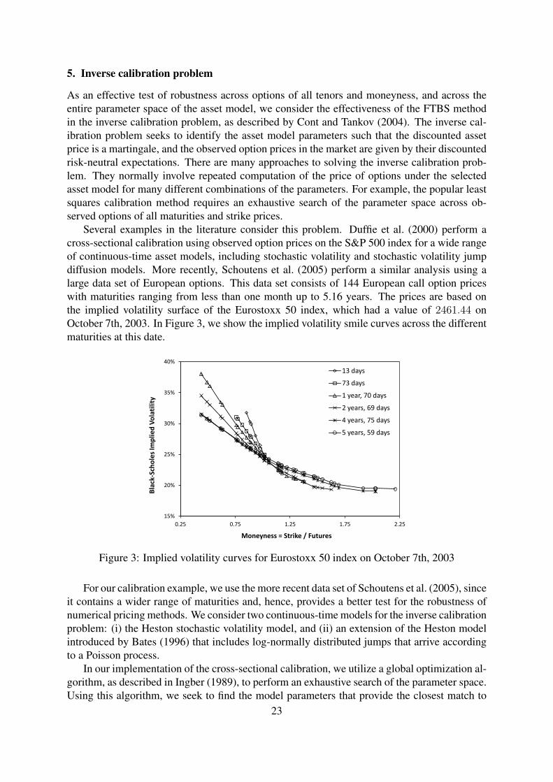
Several examples in the literature consider this problem. Duffie et al. (2000) perform across-sectional calibration using observed option prices on the S&P 500 index for a wide rangeof continuous-time asset models, including stochastic volatility and stochastic volatility jumpdiffusion models. More recently, Schoutens et al. (2005) perform a similar analysis using alarge data set of European options. This data set consists of 144 European call option priceswith maturities ranging from less than one month up to 5.16 years. The prices are based onthe implied volatility surface of the Eurostoxx 50 index, which had a value of 2461.44 onOctober 7th, 2003. In Figure 3, we show the implied volatility smile curves across the differentmaturities at this date.

15%

20%

25%

30%

35%

40%

0.25 0.75 1.25 1.75 2.25

Bla

ck-S

cho

les

Imp

lied

Vo

lati

lity

Moneyness = Strike / Futures

13 days

73 days

1 year, 70 days

2 years, 69 days

4 years, 75 days

5 years, 59 days

Figure 3: Implied volatility curves for Eurostoxx 50 index on October 7th, 2003

For our calibration example, we use the more recent data set of Schoutens et al. (2005), sinceit contains a wider range of maturities and, hence, provides a better test for the robustness ofnumerical pricing methods. We consider two continuous-time models for the inverse calibrationproblem: (i) the Heston stochastic volatility model, and (ii) an extension of the Heston modelintroduced by Bates (1996) that includes log-normally distributed jumps that arrive accordingto a Poisson process.

In our implementation of the cross-sectional calibration, we utilize a global optimization al-gorithm, as described in Ingber (1989), to perform an exhaustive search of the parameter space.Using this algorithm, we seek to find the model parameters that provide the closest match to

23

the observed implied volatility surface, subject to the Feller condition, 2κvθv ≤ σ2v , being sat-

isfied to ensure positivity of the asset price process. The inverse calibration problem thereforeprovides an excellent test for the robustness of the FTBS method as it requires accurate pricingat all maturities, strikes, and combinations of the model parameters. For comparison, we alsoconsider the same problem tackled by the FFT and the FRFT.

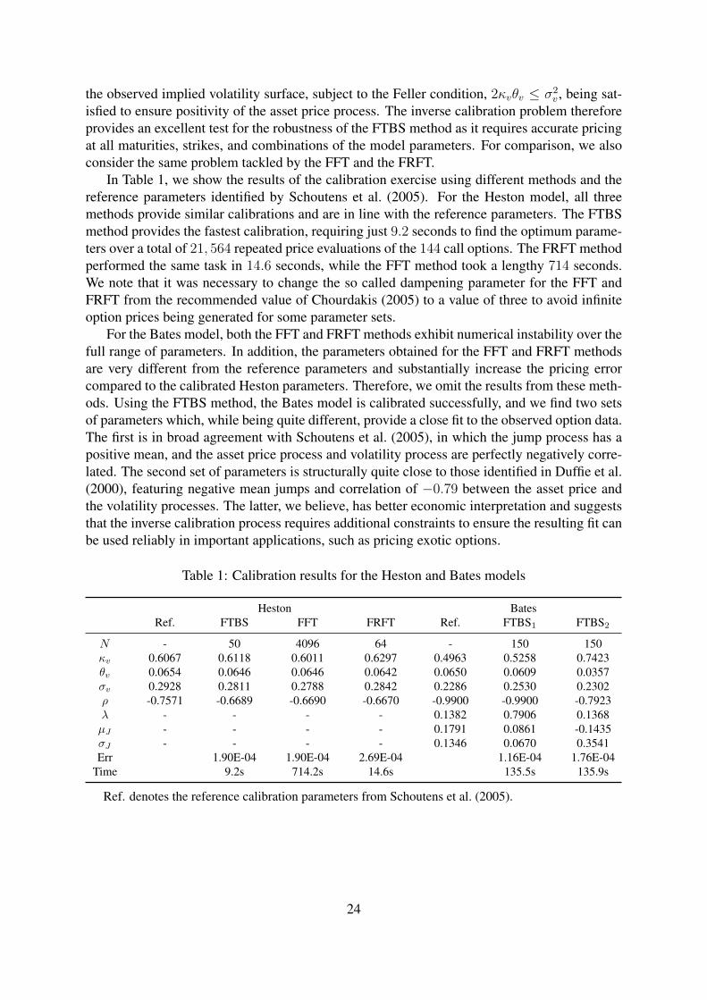
In Table 1, we show the results of the calibration exercise using different methods and thereference parameters identified by Schoutens et al. (2005). For the Heston model, all threemethods provide similar calibrations and are in line with the reference parameters. The FTBSmethod provides the fastest calibration, requiring just 9.2 seconds to find the optimum parame-ters over a total of 21, 564 repeated price evaluations of the 144 call options. The FRFT methodperformed the same task in 14.6 seconds, while the FFT method took a lengthy 714 seconds.We note that it was necessary to change the so called dampening parameter for the FFT andFRFT from the recommended value of Chourdakis (2005) to a value of three to avoid infiniteoption prices being generated for some parameter sets.

For the Bates model, both the FFT and FRFT methods exhibit numerical instability over thefull range of parameters. In addition, the parameters obtained for the FFT and FRFT methodsare very different from the reference parameters and substantially increase the pricing errorcompared to the calibrated Heston parameters. Therefore, we omit the results from these meth-ods. Using the FTBS method, the Bates model is calibrated successfully, and we find two setsof parameters which, while being quite different, provide a close fit to the observed option data.The first is in broad agreement with Schoutens et al. (2005), in which the jump process has apositive mean, and the asset price process and volatility process are perfectly negatively corre-lated. The second set of parameters is structurally quite close to those identified in Duffie et al.(2000), featuring negative mean jumps and correlation of −0.79 between the asset price andthe volatility processes. The latter, we believe, has better economic interpretation and suggeststhat the inverse calibration process requires additional constraints to ensure the resulting fit canbe used reliably in important applications, such as pricing exotic options.

Table 1: Calibration results for the Heston and Bates models

Heston BatesRef. FTBS FFT FRFT Ref. FTBS1 FTBS2

N - 50 4096 64 - 150 150κv 0.6067 0.6118 0.6011 0.6297 0.4963 0.5258 0.7423θv 0.0654 0.0646 0.0646 0.0642 0.0650 0.0609 0.0357σv 0.2928 0.2811 0.2788 0.2842 0.2286 0.2530 0.2302ρ -0.7571 -0.6689 -0.6690 -0.6670 -0.9900 -0.9900 -0.7923λ - - - - 0.1382 0.7906 0.1368µJ - - - - 0.1791 0.0861 -0.1435σJ - - - - 0.1346 0.0670 0.3541Err 1.90E-04 1.90E-04 2.69E-04 1.16E-04 1.76E-04

Time 9.2s 714.2s 14.6s 135.5s 135.9s

Ref. denotes the reference calibration parameters from Schoutens et al. (2005).

24

6. Conclusion

In this paper, we have presented an entirely new approach to approximating European-styleoption prices that utilizes B-spline interpolation theory to provide an efficient closed-form so-lution. Our framework works across the family of continuous-time exponential semimartingaleprocesses and other models whose characteristic function satisfies certain regularity constraints.Our novel use of the Peano representation of a divided difference makes the FTBS methodextremely efficient. It enables us to evaluate the pricing integral in closed-form once the inte-grands have been replaced by the B-spline approximants.

Through a very careful comparison to other methods in the literature, we have demonstratedthat the FTBS method provides accurate prices across the most widely adopted continuous-timeasset models and can provide computation times as low as one to two microseconds per optionwhen pricing a basket of options across a range of strike prices. Based on our numerical study,we can conclude that the FTBS method is the preferable approximation method, relative to theother methods considered, for computing option prices across multiple strikes prices for the VGprocess, and for the Heston model and KoBoL (CGMY) model, for precision up to the level of1E-6.

The applications of the FTBS framework are therefore wide ranging and will enable morerealistic asset models to be utilized in areas of finance in which computation time is a keyconsideration. For example, pricing, marking, and hedging of large derivative portfolios aswell as high frequency trading are all areas that can benefit from accurate real-time pricingunder realistic continuous-time asset models.

We believe that our method also has useful applications in parameter estimation in econo-metrics, when calibration incorporates cross-sectional option price information. We have pro-vided a simple example of this by calibrating the Heston and Bates models to cross-sectionaloption data. We have demonstrated the robustness of the FTBS method over the full range ofmaturities and moneyness of options as well as the full model parameter space. The FTBSmethod also has applications in maximum likelihood estimation, such as that considered byKimmel et al. (2007), in which cross-sectional information is incorporated and which requirescomputation of option prices at each iteration of the likelihood search.

Acknowledgments

We would like to thank Sergei Levendorskiı and Jiayao Xie for kindly providing their Matlabcode for the IAC method, and the two anonymous referees for their valuable comments andsuggestions which helped to significantly improve the revised version of our paper.

25

Appendix A. Fourier transform

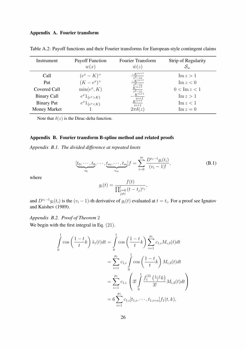
Table A.2: Payoff functions and their Fourier transforms for European-style contingent claims

Instrument Payoff Function Fourier Transform Strip of Regularityw(x) w(z) Sw

Call (ex −K)+ −Kiz+1

z2−iz Im z > 1

Put (K − ex)+ −Kiz+1

z2−iz Im z < 0

Covered Call min(ex, K) Kiz+1

z2−iz 0 < Im z < 1

Binary Call ex1ex>K −Kiz+1

iz+1Im z > 1

Binary Put ex1ex<KKiz+1

iz+1Im z < 1

Money Market 1 2πδ(z) Im z = 0

Note that δ(z) is the Dirac-delta function.

Appendix B. Fourier transform B-spline method and related proofs

Appendix B.1. The divided difference at repeated knots

[t0, · · · , t0︸ ︷︷ ︸v0

, · · · , tm, · · · , tm︸ ︷︷ ︸vm

]f =m∑i=0

Dvi−1gi(ti)

(vi − 1)!, (B.1)

where

gi(t) =f(t)∏l

j=0j 6=i

(t− tj)vj,

and Dvi−1gi(ti) is the (vi− 1)-th derivative of gi(t) evaluated at t = ti. For a proof see Ignatovand Kaishev (1989).

Appendix B.2. Proof of Theorem 2

We begin with the first integral in Eq. (21).

1∫0

cos

(1− tt

k

)s1(t)dt =

1∫0

cos

(1− tt

k

) p1∑i=1

c1,iMi,3(t)dt

=

p1∑i=1

c1,i

1∫0

cos

(1− tt

k

)Mi,3(t)dt

=

p1∑i=1

c1,i

3!

1∫0

f(3)1

(1−ttk)

3!Mi,3(t)dt

= 6

p1∑i=1

c1,i[t1,i, · · · , t1,i+n]f1(t, k),

26

where f1 is chosen to satisfy f (3)1 (1−t

tk) = cos(1−t

tk) and we have applied the Peano represen-

tation of the divided difference. We identify f1 through repeated integration of cos(1−ttk) with

respect to t. This is easily performed using symbolic integration in tools such as Mathematicaand yields the result presented in Theorem 2. The formula in Eq. (C.6) follows from Eq. (23)noting that the cosine is equal to one for k = 0 and the integral of a B-spline is also one. Theproof for the second integral is similar and is therefore omitted.

Appendix B.3. Proof of Proposition 3 (FTBS Lookback Option Price Error Bound)From (Theorem 1, formula for the price C(T,K) ) we have∣∣∣C(T,K)− C(T,K)

∣∣∣ ==

∣∣∣∣−√S0K

πe

(r+q)T2

(∫ 1

0

cos

(1− tt

k

)(s1(t)− s1(t)) dt+

∫ 1

0

sin

(1− tt

k

)(s2(t)− s2(t)) dt

)∣∣∣∣≤√S0K

πe

(r+q)T2

(∫ 1

0

∣∣∣∣cos(1− tt

k

)(s1(t)− s1(t))

∣∣∣∣ dt+ ∫ 1

0

∣∣∣∣cos(1− tt

k

)(s1(t)− s1(t))

∣∣∣∣ dt)≤√S0K

πe

(r+q)T2

(maxt∈[0,1]

|s1(t)− s1(t)|∫ 1

0

∣∣∣∣cos(1− tt

k

)∣∣∣∣ dt+max

t∈[0,1]|s2(t)− s2(t)|

∫ 1

0

∣∣∣∣sin(1− tt

k

)∣∣∣∣ dt)≤√S0K

πe

(r+q)T2

(∥∥∥s(3)1 (t)∥∥∥C1

∫ 1

0

∣∣∣∣cos(1− tt

k

)∣∣∣∣ dt+ ∥∥∥s(3)2 (t)∥∥∥C2

∫ 1

0

∣∣∣∣sin(1− tt

k

)∣∣∣∣ dt)which is the asserted bound noting that C1 = C1

∫ 1

0

∣∣cos(

1−ttk)∣∣dt and

C2 = C2

∫ 1

0

∣∣sin (1−ttk)∣∣ dt. In the last inequality we have used the optimal spline interpolation

bounds maxt∈[0,1]

|(si(t)− si(t))| = ‖si(t)− si(t)‖ ≤ Ci

∥∥∥s(3)i (t)

∥∥∥ , i = 1, 2 obtained by Gaffney

and Powell (1976). The rate O (|η|3 ) in (26) now follows applying to (25) a result by De Boor(2001) (Theorem 22, page 154). This completes the proof of Proposition 3.

Appendix B.4. Explicit formula for divided differences at repeated knotsWe begin by noting that while functions fl(t, k), l = 1, 2, are undefined at t = 0, their limit ast→ 0 exists. Therefore, in computing the divided differences at the repeated knot zero, we settl,1 = tl,2 = tl,3 = ε > 0, l = 1, 2, and consider the limit of the divided differences as ε→ 0.

27

Proposition 5. Divided difference of [ε, ε, ε, t1,4] f1

This is given by

[ε, ε, ε, t1,4] f1 =1

12ε3(ε− t1,4)3

(ε3kCi

(k

t1,4

)(6kt1,4 cos(k)−

(k2 − 6t21,4

)sin(k)

)+

ε3kCi

(k

ε

)((k2 − 6t21,4

)sin(k)− 6kt1,4 cos(k)

)+

k

(ε3(

Si(k

t1,4

)− Si

(k

ε

))((k2 − 6t21,4

)cos(k) +

6kt1,4 sin(k))− k(ε− t1,4) sinc

(k

ε

)(cos(k)

(−6ε2t1,4 + 2εk2 − k2t1,4

)+

6ε2k sin(k)))

+ ε3 cos(k)

(ε(2ε2 − 6εt1,4 − k2 + 6t21,4

)cos

(k

ε

)+

t1,4(k2 − 2t21,4

)cos

(k

t1,4

))+ ε

(ε3k(ε− 6t1,4) sin(k) cos

(k

ε

)+

ε2t1,4 sin

(k

t1,4

)((k2 − 2t21,4

)sin(k)− 5kt1,4 cos(k)

)+

5ε2kt21,4 sin(k) cos

(k

t1,4

)+ sin

(k

ε

)(k cos(k)

(−ε4 + 2ε2

(k2 +

3t21,4)− 3εk2t1,4 + k2t21,4

)+ ε2 sin(k)

(2ε3 − 6t1,4

(ε2 + k2

)+ 5εk2 + 6εt21,4

)))).

(B.2)

PROOF. The simplest way to compute the divided difference with repeated knots is by usingMathematica or a similar symbolic algebraic software package. The result in Eq. (B.2) can begenerated using the following expression in Mathematica

f1[t_] :=1/12 (k CosIntegral[k/t] (-6 k t Cos[k] + (k^2 - 6 t^2) Sin[k]) +

t (-(k^2 - 2 t^2) Cos[(k (-1 + t))/t] -5 k t Sin[(k (-1 + t))/t]) -

k ((k^2 - 6 t^2) Cos[k] + 6 k t Sin[k]) SinIntegral[k/t]);g0[t0_, t1_] := f1[t0]/(t0 - t1);g1[t0_, t1_] := f1[t1]/(t1 - t0)^3;FullSimplify[1/2*D[g0[\[Epsilon], t14], \[Epsilon], 2] +

g1[\[Epsilon], t14]]

Similar logic is used to compute the other divided differences [ε, ε, tl,4, tl,5]fl,[tl,pl−1

, tl,pl , 1, 1]fl, and [tl,pl , 1, 1, 1]fl for l = 1, 2.

In the case of divided differences with repeated arguments, [ε, ε, ε, t1,4] f1, [ε, ε, ε, t2,4] f2,[ε, ε, t1,4, t1,5] f1, and [ε, ε, t2,4, t2,5] f2, we are concerned with their limits as ε → 0. The latterare easily determined, noting in particular that limx→±∞Ci(x) = 0, limx→±∞ Si(x) = ±π

2, and

limx→±∞ Sinc(x) = 0. This leads to the following simplification of Eq. (B.2) as ε→ 0

28

(B.3)

[0, 0, 0, t1,4] f1 =1

24t31,4

(−10At21,4 sin

[A(−1 + t1,4)

t1,4

]+

2ACi

[Sign[A]At1,4

] ((A2 − 6t21,4

)sinA− 6At1,4 cosA

)− 2t1,4

(A2 − 2t21,4

)cos

[A(−1 + t1,4)

t1,4

]+

A(6At1,4 sin[A] +

(A2 − 6t21,4

)cosA

)(Sign[A]π − 2 Si

[A

t1,4

])).

Similar analysis leads to the following expressions for the other repeated divided differences atzero.

[0, 0, 0, t2,4] f2 =1

24t32,4

(−10At22,4 cos

[A(−1 + t2,4)

t2,4

]+ 2ACi

[A

t2,4

] ((A2 − 6t22,4

)cosA+

6At2,4 sinA)+ 2t2,4

(A2 − 2t22,4

)sin

[A(−1 + t2,4)

t2,4

]−A

(−6At2,4 cosA+

(A2 − 6t22,4

)sinA

)(Sign[A]π − 2 Si

[A

t2,4

])),

(B.4)

[0, 0, t1,4, t1,5] f1 =1

24t21,4(t1,4 − t1,5)t21,5

(Sign[A]A3π

(−t21,4 + t21,5

)cosA+

2t1,4t1,5

(−(A2 − 2t21,4

)t1,5 cos

[A(−1 + t1,4)

t1,4

]+

t1,4(A2−2t21,5

)cos

[A(−1 + t1,5)

t1,5

])+2A

(t21,5 Ci

[Sign[A]A

t1,4

] (−6At1,4 cosA+

(A2 − 6t21,4

)sinA

)+ t21,4 Ci

[Sign[A]At1,5

] (6At1,5 cosA−

(A2 − 6t21,5

)sinA

)+

t1,5

(t1,4

(Sign[A]3Aπ(−t1,4 + t1,5) sinA+ 5t1,4t1,5

(sin

[A

(−1 +

1

t1,4

)]+ sin

[A(−1 + t1,5)

t1,5

]))− t1,5

((A2 − 6t21,4

)cosA+

6At1,4 sinA)Si

[A

t1,4

])+ t21,4

((A2 − 6t21,5

)cosA+ 6At1,5 sinA

)Si

[A

t1,5

])),

(B.5)

29

(B.6)

[0, 0, t2,4, t2,5] f2 =1

24t22,4(t2,4 − t2,5)t22,5

(2At2,4t2,5

(Sign[A] ∗ 3Aπ(−t2,4 + t2,5) cosA+

5t2,4t2,5

(− cos

[A(−1 + t2,4)

t2,4

]+ cos

[A(−1 + t2,5)

t2,5

]))+

Sign[A] ∗A3πt22,4 sinA− Sign[A] ∗A3πt22,5 sinA+

2At22,5 Ci

[A

t2,4

] ((A2 − 6t22,4

)cosA+

6At2,4 sinA)− 2At22,4 Ci

[A

t2,5

] ((A2 − 6t22,5

)cosA+ 6At2,5 sinA

)+

2A2t2,4t22,5 sin

[A(−1 + t2,4)

t2,4

]− 4t32,4t

22,5 sin

[A(−1 + t2,4)

t2,4

]− 2t22,4t2,5

(A2 − 2t22,5

)sin

[A(−1 + t2,5)

t2,5

]+

2A

(t22,5(−6At2,4 cosA+

(A2 − 6t22,4

)sinA

)Si

[A

t2,4

]+

t22,4(6At2,5 cosA−A2 sinA+ 6t22,5 sinA

)Si

[A

t2,5

])).

Appendix C. The FTBS method for alternative contour integrals

Theorem 3 (Strike-separable pricing formula). An alternative form of Eq. (5) for comput-ing C(T,K) is given by

C(T,K) = −Ke−rT+vk

πI(k; v) (C.1)

where

I(k; v) =

1∫0

cos

(1− tt

k

)s1(t; v)dt+

1∫0

sin

(1− tt

k

)s2(t; v)dt

s1(t; v) =Re[φXT

(−1−tt− iv)

] [(1−tt

)2+ v − v2

]+ Im

[φXT

(−1−tt− iv)

] (1−tt

)(2v − 1)

t2(

[(

1−tt

)2+ v − v2]2 +

(1−tt

)2(2v − 1)2

)s2(t; v) =

−Re[φXT

(−1−tt− iv)

] (1−tt

)(2v − 1) + Im

[φXT

(−1−tt− iv)

] [(1−tt

)2+ v − v2

]t2(

[(

1−tt

)2+ v − v2]2 +

(1−tt

)2(2v − 1)2

)and v ∈ (1, α), as in Proposition 1.

PROOF. Note that since the option price provided by the integral in Eq. (2) is real-valued, wecan rewrite it as

C(T,K) = −Ke−rT

2π

iv+∞∫iv−∞

Re

[φXT

(−z)e−izk

z2 − iz

]dz, with v ∈ (1, α),

We now denote the real and imaginary parts of φXT(−z) as φRe(z1, v) and φIm(z1, v) so that

φXT(−z) = φXT

(−(z1 + iv)) = φRe(z1, v) + iφIm(z1, v)30

where z1 ∈ (−∞,∞) along the integration path. For brevity, we write φRe and φIm, instead ofφRe(z1, v) and φIm(z1, v), keeping in mind that these are functions of z1 and v. We now rewritee−izk,

e−izk = e−i(z1+iv)k = evke−iz1k = evk [cos (z1k)− i sin (z1k)] .

Therefore (2) becomes

C(T,K) = −Ke−rT

2π

∞∫−∞

Re

(φRe + iφIm)evk [cos (z1k)− i sin (z1k)]

(z1 + iv)2 − i(z1 + iv)︸ ︷︷ ︸(∗)

dz1 (C.2)

We expand (∗) into its real and imaginary parts

(∗) = z21 + 2ivz1 − v2 − iz1 + v = z2

1 + v − v2 + iz1(2v − 1)

Multiplying the numerator and denominator of the integrand in Eq. (C.2) by the complexcongruent of (∗) provides

C(T,K) =−Ke−rT+vk

2π

∞∫−∞

Re

a1+a2i︷ ︸︸ ︷

(φRe+iφIm)

b1−b2i︷ ︸︸ ︷[cos (z1k)−i sin (z1k)]

c1−c2i︷ ︸︸ ︷(z2

1 +v−v2−iz1(2v−1))

(z21 + v − v2)2 + z2

1(2v − 1)2

dz1.

Now, noting that Re[(a1 + a2i)(b1 − b2i)(c1 − c2i)] = a1b1c1 + a2b2c1 + a2b1c2 − a1b2c2, wehave the following expression for the pricing integral

C(T,K) = −Ke−rT+vk

2π

∞∫−∞

cos (z1k) [φRe (z21 + v − v2) + φImz1(2v − 1)]

(z21 + v − v2)2 + z2

1(2v − 1)2dz1

+

∞∫−∞

sin (z1k) [−φRez1(2v − 1) + φIm (z21 + v − v2)]

(z21 + v − v2)2 + z2

1(2v − 1)2dz1

. (C.3)

In order to simplify Eq. (C.3), we now show that the integrands in Eq. (C.3) are evenfunction with respect to z1. Examining the characteristic function of XT along the integrationpath shows that

φXT(−z) = EQ

(e−izXT

)= EQ

(e−i(z1+iv)XT

)= EQ

(e−iz1XT e

vXn)

= EQ(evXn [cos(−z1) + i sin(−z1)]

), since XT ∈ R

= EQ(evXn [cos(z1)− i sin(z1)]

)= EQ

(evXn cos(z1)

)− iEQ

(evXn sin(z1)

)= φRe(z1, v) + iφIm(z1, v),

31

where φRe and φIm are as defined in Eq. (C.3). Observe that φRe(z1, v) = φRe(−z1, v) andφIm(z1, v) = −φIm(−z1, v), so that the real part of φXT

(−z) is even and the imaginary part isodd. Now, in (C.3), denote the first integrand by f1(z1, v) and the second by f2(z1, v) so that

C(T,R) = −R1−v

2π

∞∫−∞

f1(z1, v)dz1 +

∞∫−∞

f2(z1, v)dz1

.By inspection, using the even property of φRe and cosine, and the odd property of φIm and sine,we have that both f1(z1, v) = f1(−z1, v) and f2(z1, v) = f2(−z1, v).

Using this even function property we can modify the integration limits of (C.3) to [0,∞),noting the even function property and scaling by a factor of 2. We then make the substitutionz1 = 1−t

tin Eq. (C.3) which provides the required result.

Theorem 4 (The FTBS pricing formula for alternative contour integrals).Let t1,i6+l1

i=1 , t2,j6+l2j=1 and c1,i(v)p1

i=1, c2,j(v)p2

j=1 be the sets of knots and linear coeffi-cients of s1(t; v) and s2(t; v) respectively, which are the the quadratic spline interpolants offunctions s1(t; v) and s2(t; v), as specified in Theorem 3, where p1 = l1 + 3 and p2 = l2 + 3.Additionally, let k = log

(S0

K

)+ (r − q)T , and v ∈ (1, α), as in Proposition 1. The pricing

formula of a European call option is given as

C(T,K) ≈ −Ke−rT+vk

πI(k; v), (C.4)

where for k 6= 0

I(k; v) = 6

p1∑i=1

c1,i(v)[t1,i, t1,i+1, t1,i+2, t1,i+3]f1(t, k)

+ 6

p2∑i=1

c2,i(v)[t2,i, t2,i+1, t2,i+2, t2,i+3]f2(t, k), (C.5)

and f1 and f2 are defined as in Theorem 2. For k = 0, I(k; v) simplifies to

I(k; v) =

p1∑i=1

c1,i(v) +

p2∑i=1

c2,i(v). (C.6)

PROOF. The proof utilizes Eq. (C.1) of Theorem 3, and is similar to that Theorem 2, andtherefore is omitted.

32

Appendix D. Numerical implementation of pricing methods

The FFT and FRFT methods:Our implementation of the FFT and FRFT methods carefully follows the description of Chour-dakis (2005), and utilizes the numerical library of Frigo and Johnson (1998) in C++, which isknown to be one of the fastest implementations of the FFT available. Under the FFT and FRFT,it is necessary to truncate the upper limit of the Fourier integral and select the number of gridpoints for the numerical computation. We follow the recommendations of Chourdakis (2005)in configuring each of the methods for the respective asset models.

The COS method:Our implementation of the COS method precisely follows the description provided in Fangand Oosterlee (2008). In particular, we have utilized Eq. (30) in Fang and Oosterlee (2008),which enables option prices for different strikes to be obtained in one single numerical exper-iment. The COS method requires a truncation limit for integration, and we have followed therecommendation L = 10, specified in Eq. (49) and the calculation of the cumulants specifiedin Table 11, both in Fang and Oosterlee (2008). We note that in the case of the Heston model,we use only the first and second cumulant in defining the truncation range, as recommendedby Fang and Oosterlee (2008). Finally, we note that following Remark 5.2 of Fang and Oost-erlee (2008), we have computed put option prices, and used the put-call parity to compute therequired call option prices. This is noted to remove sensitivity with respect to the choice of thetruncation parameter L.

The IAC method:We have implemented the IAC method using the enhanced Simpson rule for the VG processdescribed in Levendorskiı and Xie (2012). We thank Sergei Levendorskiı and Jiayao Xie forkindly providing their Matlab code which we directly converted into C++ in our implementa-tion.

The CONV method:Our implementation of the CONV method carefully follows Eq. (27) of Lord et al. (2009), andagain we utilize the numerical library of Frigo and Johnson (1998) for the computation of theFFT. We note that Eq. (27) of Lord et al. (2009) is intended for use in pricing early exerciseoptions, and therefore provides option prices across a range of initial underlying asset prices(as opposed to strike prices). Since we are not concerned with option prices at different initialasset prices, we replace the outer discrete Fourier transform in Eq. (27) of Lord et al. (2009),with a single summation corresponding to the required initial asset price. This provides theoptimal performance of the CONV method when it is applied for pricing European options ata single initial asset price.

33

Appendix E. Other numerical comparisons

We now provide further numerical comparisons to validate the numerical accuracy of the FTBSmethod for computing the Greeks, and also the accuracy of options prices under additional as-set price models.

The Greeks:We compute the Greeks of European options under the Heston model using the FTBS methodand compare them to the results of Kristensen and Mele (2011) under their Taylor expansionapproximation method. The results of our comparison of the Greeks are provided in (a), (b),(c), and (d) of Table F.9. Note that the reported exact option sensitivities are those providedin Kristensen and Mele (2011). Across all levels of initial share price and volatility, the FTBSmethod produces accurate results using only 50 data sites. Moving to 100 data sites yieldsresults to seven significant figures. The total computation time of the option price Delta’s andGamma’s in (a) and (b) of Table F.9 are just 0.02 milliseconds respectively using 50 data sitesfor the 11 initial share prices, or equivalently, under two microseconds per option. In (c) and(d) of Table F.9, the total calculation time increases to 0.84 milliseconds since we need to re-fitthe spline approximants for each initial volatility level V0. Overall, we have demonstrated thatthe FTBS method provides greater precision than the approximation method of Kristensen andMele (2011), since we have precisely matched the reference prices, while achieving computa-tion times as low as two microseconds per option.

The double exponential jump diffusion process:We consider the pricing example under the double exponential jump diffusion process of Kou(2002) that uses the enhanced FFT method described in Boyarchenko and Levendorskiı (2002).Quittard-Pinon and Randrianarivony (2010) produce the reference prices, and we provide ournumerical comparison in Table F.4. Using 500 data sites, the FTBS method produces pricesthat are in agreement with the reference prices and are more accurate than the FFT results byabout one significant figure. Our computation time is only 0.2ms in total for the 11 options.

The mixed exponential jump diffusion model:Cai and Kou (2011) report the prices of European call options under the Mixed ExponentialJump Diffusion model using the EI method of Petrella (2004). Our results are presented inTable F.5. Using 100 data sites, the FTBS method produces near identical prices. The FTBScomputation time is 0.05ms per option.

34

Appendix F. Tables

Table F.3: Recommended configuration of FTBS method for desired level of precision

Accuracy VG Heston KoBoL / CGMY

1E-4 25 25 301E-5 35 50 701E-6 200 80 1801E-7 400 170 4501E-8 - 250 1050

Above is based on numerical results from Section 4 by considering minimum number of knotsrequired for desired precision across “low”, “bench”, and “high” parameter sets.

Table F.4: Comparison to the generalized FFT method results of Quittard-Pinon and Randria-narivony (2010), C1 series, Table 2 (DEJD model)

FFT Error FTBS Error

90 -1.51E-08 6.56E-0992 -1.61E-08 1.37E-1094 -1.16E-08 -1.42E-0996 -3.77E-09 -9.51E-1098 2.02E-09 -6.65E-10

100 3.05E-08 -5.84E-10102 4.62E-08 9.19E-10104 3.28E-08 -9.62E-10106 1.53E-08 -3.82E-10108 7.86E-09 -6.95E-10110 9.25E-09 -5.71E-09

Total time 16ms 0.2msSpeed-up Factor 80×

DEJD parameters: S = 100, σ = 0.16, λ = 1, η1 = 10, η2 = 5, p = 0.4, r = 0.05, q = 0.Calculation time reported for pricing 11 options. FFT method is using N = 4096 and FTBS methoduses N = 500.

Table F.5: Comparison to the EI method results of Cai and Kou (2011), Table 1 (MEJD model)

σ = 0.2 σ = 0.3η1 λ EI Price FTBS Diff. EI Price FTBS Diff.

20 1 10.97472 10.97472 0.00000 14.59752 14.59753 0.0000120 3 11.94485 11.94485 0.00000 15.29993 15.29994 0.0000120 5 12.83076 12.83077 0.00001 15.96677 15.96678 0.0000140 1 10.57572 10.57572 0.00000 14.31636 14.31637 0.0000140 3 10.82050 10.82050 0.00000 14.48475 14.48476 0.0000140 5 11.05846 11.05845 0.00001 14.65079 14.65079 0.00000

Mixed Exponential parameters: S = 100, σ = 0.2, λ = 5, η1 = 20, θ1 = 20, η2 = 50, θ2 = 50, p =0.4, p1 = 1.2, p2 = −0.2, q1 = 1.3, q2 = −0.3, r = 0.05, q = 0, T = 1,K = 100.EI parameters A = 18, n = 30, X = 10, 000. FTBS method using N = 100.

35

TableF.6:H

estonm

odeloptionpricing

results

Low

Bench

High

Accuracy

PricingN

Mean

RM

SEA

bs.Tim

eSpeed

upN

Mean

RM

SEA

bs.Tim

eSpeed

upN

Mean

RM

SEA

bs.Tim

eSpeed

upM

ethodE

rrorE

rror(m

s)to

FFTE

rrorE

rror(m

s)to

FFTE

rrorE

rror(m

s)to

FFT

1E-04

FFT10

9.4E-06

1.6E-05

4.6E-05

1.43-

92.8E

-053.1E

-054.8E

-050.72

-8

4.7E-05

5.1E-05

7.4E-05

0.37-

FRFT

61.1E

-051.5E

-054.6E

-050.12

125

2.1E-05

2.4E-05

4.2E-05

0.0711

42.5E

-053.4E

-057.5E

-050.03

11C

OS

174.6E

-055.3E

-059.5E

-050.06

2421

3.1E-05

3.5E-05

5.4E-05

0.0710

235.2E

-055.4E

-056.7E

-050.08

5FT

BS

234.2E

-055.0E

-059.6E

-050.04

4120

8.3E-05

8.3E-05

9.5E-05

0.0324

218.7E

-058.7E

-059.0E

-050.03

11

1E-05

FFT11

2.5E-06

3.8E-06

1.0E-05

2.86-

105.8E

-066.9E

-061.1E

-051.48

-9

1.1E-05

1.2E-05

1.8E-05

0.73-

FRFT

85.7E

-071.1E

-063.0E

-060.46

66

3.4E-06

4.5E-06

1.0E-05

0.1212

51.1E

-051.2E

-051.8E

-050.07

11C

OS

227.5E

-068.3E

-061.3E

-050.08

3724

1.0E-05

1.1E-05

1.7E-05

0.0818

261.3E

-051.4E

-052.0E

-050.09

8FT

BS

444.7E

-065.5E

-061.1E

-050.06

4522

9.6E-06

9.7E-06

1.1E-05

0.0345

321.7E

-051.7E

-051.8E

-050.05

15

1E-06

FFT12

9.0E-07

1.0E-06

2.0E-06

5.91-

118.5E

-079.9E

-072.0E

-062.96

-11

5.0E-07

6.2E-07

1.1E-06

2.89-

FRFT

85.9E

-071.1E

-063.0E

-060.46

137

1.7E-06

2.0E-06

3.0E-06

0.2313

78.1E

-079.0E

-071.2E

-060.23

13C

OS

261.1E

-061.2E

-061.8E

-060.09

6329

6.4E-07

7.3E-07

1.3E-06

0.1029

311.0E

-061.1E

-061.6E

-060.11

26FT

BS

756.4E

-077.7E

-071.5E

-060.10

5736

1.4E-06

1.4E-06

1.5E-06

0.0558

601.2E

-061.2E

-061.3E

-060.08

35

1E-07

FFT14

1.4E-07

1.6E-07

1.9E-07

23.10-

131.5E

-071.8E

-073.1E

-0711.55

-12

1.1E-07

1.2E-07

1.9E-07

5.72-

FRFT

119.7E

-091.6E

-084.3E

-083.77

610

3.3E-08

3.6E-08

5.2E-08

1.777

94.3E

-084.8E

-087.4E

-080.90

6C

OS

312.4E

-082.8E

-084.8E

-080.11

21035

2.0E-08

2.2E-08

3.5E-08

0.1392

374.2E

-084.6E

-087.1E

-080.14

42FT

BS

1653.0E

-083.8E

-088.6E

-080.22

10560

3.9E-08

4.3E-08

8.9E-08

0.09132

1109.7E

-089.7E

-081.0E

-070.15

38

1E-08

FFT14

1.4E-07

1.6E-07

1.9E-07

22.41-

131.5E

-071.8E

-073.1E

-0711.18

-13

5.5E-08

6.5E-08

1.1E-07

10.94-

FRFT

122.6E

-094.4E

-091.3E

-087.03

311

4.8E-09

5.8E-09

1.1E-08

3.623

118.7E

-098.9E

-091.1E

-083.49

3C

OS

341.2E

-081.4E

-082.1E

-080.12

19238

6.7E-09

7.6E-09

1.2E-08

0.1384

391.3E

-081.5E

-082.3E

-080.14

78FT

BS

2505.0E

-096.6E

-091.6E

-080.33

68100

1.1E-08

1.1E-08

1.3E-08

0.1483

1701.6E

-081.6E

-081.7E

-080.23

47

Option

pricingparam

etersunderH

estonm

odel:L

ow.

S0=

1,V0=

0.01,κ

=1.0,θ

=0.09,σ

=0.05,ρ

=−0.5,r

=q=

0,T=

0.1.B

ench.S

0=

1,V0=

0.09,κ=

3.0,θ

=0.09,σ

=0.15,ρ

=−0.5,r

=q=

0,T=

0.25.H

igh.S

0=

1,V0=

0.81,κ

=9.0,θ

=0.09,σ

=0.45,ρ

=−0.5,r

=q=

0,T=

1.U

pperintegrationlim

itsforFFT

andFR

FTchosen

optimally

tom

inimize

pricingerror.

Calculation

time

reportedforpricing

31options

with

K=

0.85to

1.15

insteps

of0.01.

36

Tabl

eF.

7:V

aria

nce

gam

ma

proc

ess

optio

npr

icin

gre

sults

Low

Ben

chH

igh

Acc

urac

yPr

icin

gN

Mea

nR

MSE

Abs

.Ti

me

Spee

dup

NM

ean

RM

SEA

bs.

Tim

eSp

eed

upN

Mea

nR

MSE

Abs

.Ti

me

Spee

dup

Met

hod

Err

orE

rror

(ms)

vs.F

FTE

rror

Err

or(m

s)vs

.FFT

Err

orE

rror

(ms)

vs.F

FT

1E-0

4FF

T10

8.9E

-06

1.7E

-05

6.2E

-05

0.60

-9

3.0E

-05

3.5E

-05

7.1E

-05

0.31

-9

3.9E

-05

4.4E

-05

7.2E

-05

0.31

-FR

FT7

9.0E

-05

9.0E

-05

9.9E

-05

0.12

55

3.5E

-05

4.1E

-05

8.0E

-05

0.05

74

4.3E

-05

5.2E

-05

1.1E

-04

0.02

17C

OS

272.

1E-0

52.

6E-0

57.

0E-0

50.

078

305.

2E-0

56.

0E-0

51.

2E-0

40.

084

205.

2E-0

55.

9E-0

59.

4E-0

50.

065

FTB

S21

1.2E

-05

1.5E

-05

2.7E

-05

0.01

4320

9.2E

-05

9.2E

-05

1.0E

-04

0.01

2321

6.0E

-05

6.0E

-05

6.2E

-05

0.01

22

1E-0

5FF

T11

2.2E

-06

3.6E

-06

1.1E

-05

1.23

-12

1.6E

-06

2.0E

-06

4.4E

-06

2.54

-12

2.8E

-06

3.2E

-06

4.8E

-06

2.50

-FR

FT8

6.3E

-06

6.4E

-06

8.8E

-06

0.25

56

6.5E

-06

7.8E

-06

1.7E

-05

0.07

386

2.8E

-06

3.1E

-06

4.8E

-06

0.07

37C

OS

506.

3E-0

69.

1E-0

62.

7E-0

50.

149

603.

4E-0

64.

2E-0

69.

1E-0

60.

1616

285.

1E-0

65.

7E-0

69.

7E-0

60.

0833

FTB

S32

2.3E

-06

3.1E

-06

9.9E

-06

0.02

6131

2.1E

-06

2.5E

-06

5.0E

-06

0.02

128

337.

1E-0

67.

1E-0

67.

4E-0

60.

0211

7

1E-0

6FF

T13

2.3E

-07

3.7E

-07

9.7E

-07

4.77

-13

2.7E

-07

3.1E

-07

6.7E

-07

5.07

-13

4.0E

-07

4.6E

-07

7.7E

-07

4.82

-FR

FT10

7.9E

-08

1.2E

-07

3.6E

-07

0.93

58

4.6E

-07

5.2E

-07

8.2E

-07

0.25

208

1.5E

-07

1.8E

-07

3.1E

-07

0.25

20C

OS

506.

3E-0

69.

1E-0

62.

7E-0

50.

1336

100

1.2E

-06

1.5E

-06

3.0E

-06

0.28

1840

3.9E

-07

4.4E

-07

7.3E

-07

0.11

45FT

BS

170

1.5E

-07

2.7E

-07

8.5E

-07

0.09

5295

2.7E

-07

3.6E

-07

9.8E

-07

0.05

9460

8.8E

-07

8.8E

-07

9.0E

-07

0.03

139

1E-0

7FF

T15

7.4E

-08

1.0E

-07

2.3E

-07

20.1

4-

147.

5E-0

88.

8E-0

81.

7E-0

79.

87-

148.

3E-0

89.

6E-0

81.

5E-0

79.

80-

FRFT

105.

5E-0

88.

4E-0

82.

8E-0

70.

9521

96.

5E-0

87.

7E-0

81.

4E-0

70.

4721

94.

2E-0

84.

7E-0

87.

6E-0

80.

4621

CO

S50

6.3E

-06

9.1E

-06

2.7E

-05

0.13

153

220

1.2E

-06

1.5E

-06

3.0E

-06

0.28

1710

07.

8E-0

88.

4E-0

81.

4E-0

70.

2736

FTB

S38

06.

7E-0

88.

7E-0

81.

9E-0

70.

2010

233

01.

8E-0

83.

0E-0

89.

7E-0

80.

1757

100

9.7E

-08

9.7E

-08

1.0E

-07

0.06

174

Opt

ion

pric

ing

para

met

ers

unde

rVar

ianc

ega

mm

apr

oces

s:L

ow.

S0=

1,µ=−0.1,σ

=0.15,ν

=0.1,r=q=

0,T

=0.1

.B

ench

.S

0=

1,µ=−0.2,σ

=0.3,

ν=

0.2,r=q=

0,T

=0.25

.H

igh.

S0=

1,µ=−0.3,σ

=0.45,ν=

0.3,r=q=

0,T

=1.

Upp

erin

tegr

atio

nlim

itsfo

rFFT

and

FRFT

chos

enop

timal

lyto

min

imiz

epr

icin

ger

ror.

Cal

cula

tion

time

repo

rted

forp

rici

ng31

optio

nsw

ithK

=0.85

to1.15

inst

eps

of0.01

.

37

TableF.8:K

oBoL

(CG

MY

)processoption

pricingresults

Low

Bench

High

Accuracy

PricingN

Mean

RM

SEA

bs.Tim

eSpeed

upN

Mean

RM

SEA

bs.Tim

eSpeed

upN

Mean

RM

SEA

bs.Tim

eSpeed

upM

ethodE

rrorE

rror(m

s)vs.FFT

Error

Error

(ms)

vs.FFTE

rrorE

rror(m

s)vs.FFT

1E-04

FFT8

4.9E-05

5.5E-05

9.3E-05

0.25-

81.8E

-052.1E

-053.4E

-050.25

-9

3.8E-05

4.4E-05

7.9E-05

0.50-

FRFT

56.2E

-056.9E

-051.2E

-040.05

54

3.6E-05

4.3E-05

8.6E-05

0.0210

41.5E

-041.6E

-042.0E

-040.02

22C

OS

734.2E

-055.0E

-051.0E

-040.23

143

3.7E-05

4.2E-05

7.1E-05

0.132

121.9E

-041.9E

-042.1E

-040.04

14FT

BS

263.8E

-054.3E

-058.0E

-050.03

915

8.4E-05

8.4E-05

9.1E-05

0.0215

171.5E

-041.5E

-041.6E

-040.02

27

1E-05

FFT9

7.1E-06

8.0E-06

1.5E-05

0.51-

96.0E

-066.9E

-061.2E

-050.50

-10

1.1E-05

1.3E-05

2.2E-05

0.98-

FRFT

67.7E

-069.0E

-061.8E

-050.09

55

9.0E-06

1.1E-05

1.7E-05

0.059

53.9E

-064.6E

-068.4E

-060.05

19C

OS

1293.5E

-064.4E

-069.7E

-060.40

154

6.1E-06

6.8E-06

1.1E-05

0.173

157.2E

-067.3E

-068.3E

-060.05

22FT

BS

673.8E

-064.4E

-069.6E

-060.07

830

1.1E-05

1.1E-05

1.1E-05

0.0316

302.2E

-062.4E

-064.2E

-060.03

31

1E-06

FFT11

1.5E-06

1.7E-06

2.6E-06

2.03-

102.0E

-062.2E

-063.4E

-061.00

-12

8.5E-07

9.9E-07

1.8E-06

4.29-

FRFT

72.0E

-062.3E

-063.6E

-060.17

127

6.1E-07

7.0E-07

1.1E-06

0.186

69.8E

-071.1E

-062.1E

-060.09

47C

OS

2152.8E

-073.6E

-079.2E

-070.84

269

4.4E-07

5.1E-07

8.4E-07

0.215

192.2E

-072.3E

-072.8E

-070.06

73FT

BS

1802.8E

-073.5E

-079.6E

-070.17

1250

7.0E-07

7.0E-07

7.6E-07

0.0521

402.9E

-073.4E

-074.9E

-070.04

103

1E-07

FFT13

1.3E-07

1.5E-07

2.4E-07

8.17-

134.7E

-085.4E

-089.2E

-087.95

-14

6.8E-08

7.7E-08

1.3E-07

16.60-

FRFT

91.3E

-071.6E

-072.9E

-070.71

129

4.4E-08

5.1E-08

9.6E-08

0.6812

85.3E

-086.3E

-081.3E

-070.34

48C

OS

3312.5E

-083.5E

-089.9E

-081.06

885

4.1E-08

4.7E-08

7.8E-08

0.2730

212.0E

-082.2E

-083.1E

-080.07

245FT

BS

4392.3E

-083.0E

-089.9E

-080.42

2074

4.4E-08

5.1E-08

9.1E-08

0.07113

808.6E

-088.7E

-089.7E

-080.08

208

1E-08

FFT15

1.9E-08

2.2E-08

4.3E-08

32.70-

141.5E

-081.9E

-083.8E

-0816.29

-15

2.6E-08

3.0E-08

4.6E-08

32.68-

FRFT

118.5E

-091.0E

-082.3E

-082.70

1210

2.0E-08

2.2E-08

3.2E-08

1.3612

91.5E

-081.7E

-083.3E

-080.68

48C

OS

5002.9E

-093.9E

-099.6E

-091.54

2199

4.9E-09

5.5E-09

9.3E-09

0.3054

301.7E

-081.8E

-083.0E

-080.09

354FT

BS

10101.9E

-092.9E

-099.7E

-090.94

35122

2.7E-09

3.1E-09

5.3E-09

0.12140

1509.1E

-099.1E

-099.9E

-090.14

227

Option

pricingparam

etersunderK

oBoL

(CG

MY

)model(to

7decim

alplaces):L

ow.

S0=

1,λ+=

22.9666

295,λ−=−6.9666295

,c+=c−

=5,ν

=0.25,r

=q=

0,T=

0.1.B

ench.S

0=

1,λ+=

22.9666295

,λ−=−6.9666295

,c+=c−

=5,ν

=0.5,r

=q=

0,T=

0.25.H

igh.S

0=

1,λ+=

7.63535

90,λ−=−4.3295739

,c+=c−

=5,ν

=0.5,r

=q=

0,T=

1.U

pperintegrationlim

itsforFFT

andFR

FTchosen

optimally

tom

inimize

pricingerror.

Calculation

time

reportedforpricing

31options

with

K=

0.85to

1.15

insteps

of0.01.

38

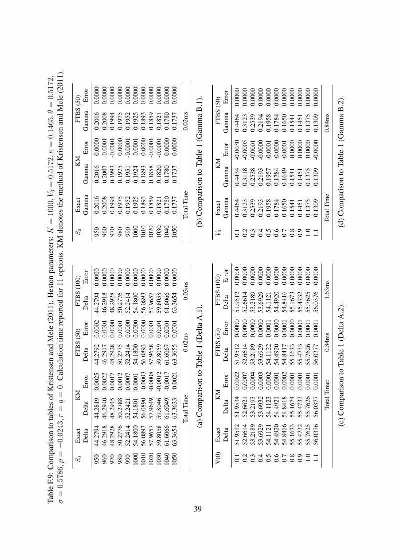
Tabl

eF.

9:C

ompa

riso

nto

tabl

esof

Kri

sten

sen

and

Mel

e(2

011)

.Hes

ton

para

met

ers:K

=10

00,V

0=

0.51

72,κ

=0.

1465,θ

=0.

5172,

σ=

0.57

86,ρ

=−

0.02

43,r

=q

=0.

Cal

cula

tion

time

repo

rted

for1

1op

tions

.KM

deno

tes

the

met

hod

ofK

rist

ense

nan

dM

ele

(201

1).

S0

Exa

ctK

MFT

BS

(50)

FTB

S(1

00)

Del

taD

elta

Err

orD

elta

Err

orD

elta

Err

or

950

44.2

794

44.2

819

0.00

2544

.279

20.

0002

44.2

794

0.00

0096

046

.291

846

.294

00.

0022

46.2

917

0.00

0146

.291

80.

0000

970

48.2

928

48.2

945

0.00

1748

.292

80.

0000

48.2

928

0.00

0098

050

.277

650

.278

80.

0012

50.2

775

0.00

0150

.277

60.

0000

990

52.2

414

52.2

421

0.00

0752

.241

40.

0000

52.2

414

0.00

0010

0054

.180

054

.180

10.

0001

54.1

800

0.00

0054

.180

00.

0000

1010

56.0

893

56.0

890

-0.0

003

56.0

893

0.00

0056

.089

30.

0000

1020

57.9

657

57.9

649

-0.0

008

57.9

658

0.00

0157

.965

70.

0000

1030

59.8

058

59.8

046

-0.0

012

59.8

059

0.00

0159

.805

80.

0000

1040

61.6

066

61.6

049

-0.0

017

61.6

067

0.00

0161

.606

60.

0000

1050

63.3

654

63.3

633

-0.0

021

63.3

655

0.00

0163

.365

40.

0000

Tota

lTim

e0.

02m

s0.

03m

s

(a)C

ompa

riso

nto

Tabl

e1

(Del

taA

.1).

S0

Exa

ctK

MFT

BS

(50)

Gam

ma

Gam

ma

Err

orG

amm

aE

rror

950

0.20

160.

2016

0.00

000.

2016

0.00

0096

00.

2008

0.20

07-0

.000

10.

2008

0.00

0097

00.

1994

0.19

93-0

.000

10.

1994

0.00

0098

00.

1975

0.19

750.

0000

0.19

750.

0000

990

0.19

520.

1951

-0.0

001

0.19

520.

0000

1000

0.19

250.

1924

-0.0

001

0.19

250.

0000

1010

0.18

930.

1893

0.00

000.

1893

0.00

0010

200.

1859

0.18

58-0

.000

10.

1859

0.00

0010

300.

1821

0.18

20-0

.000

10.

1821

0.00

0010

400.

1780

0.17

800.

0000

0.17

800.

0000

1050

0.17

370.

1737

0.00

000.

1737

0.00

00

Tota

lTim

e0.

02m

s

(b)C

ompa

riso

nto

Tabl

e1

(Gam

ma

B.1

).

V(0

)E

xact

KM

FTB

S(5

0)FT

BS

(100

)D

elta

Del

taE

rror

Del

taE

rror

Del

taE

rror

0.1

51.9

512

51.9

534

0.00

2251

.951

20.

0000

51.9

512

0.00

000.

252

.661

452

.662

10.

0007

52.6

614

0.00

0052

.661

40.

0000

0.3

53.2

189

53.2

193

0.00

0453

.218

90.

0000

53.2

189

0.00

000.

453

.692

953

.693

20.

0003

53.6

929

0.00

0053

.692

90.

0000

0.5

54.1

121

54.1

123

0.00

0254

.112

20.

0001

54.1

121

0.00

000.

654

.492

054

.492

10.

0001

54.4

920

0.00

0054

.492

00.

0000

0.7

54.8

416

54.8

418

0.00

0254

.841

70.

0001

54.8

416

0.00

000.

855

.167

355

.167

40.

0001

55.1

673

0.00

0055

.167

30.

0000

0.9

55.4

732

55.4

733

0.00

0155

.473

30.

0001

55.4

732

0.00

001.

055

.762

555

.762

60.

0001

55.7

626

0.00

0155

.762

50.

0000

1.1

56.0

376

56.0

377

0.00

0156

.037

70.

0001

56.0

376

0.00

00

Tota

lTim

e:0.

84m

s1.

63m

s

(c)C

ompa

riso

nto

Tabl

e1

(Del

taA

.2).

V0

Exa

ctK

MFT

BS

(50)

Gam

ma

Gam

ma

Err

orG

amm

aE

rror

0.1

0.44

640.

4434

-0.0

030

0.44

640.

0000

0.2

0.31

230.

3118

-0.0

005

0.31

230.

0000

0.3

0.25

390.

2538

-0.0

001

0.25

390.

0000

0.4

0.21

930.

2193

-0.0

000

0.21

940.

0000

0.5

0.19

580.

1957

-0.0

001

0.19

580.

0000

0.6

0.17

840.

1784

-0.0

000

0.17

840.

0000

0.7

0.16

500.

1649

-0.0

001

0.16

500.

0000

0.8

0.15

410.

1541

0.00

000.

1541

0.00

000.

90.

1451

0.14

510.

0000

0.14

510.

0000

1.0

0.13

750.

1375

0.00

000.

1375

0.00

001.

10.

1309

0.13

09-0

.000

00.

1309

0.00

00

Tota

lTim

e0.

84m

s

(d)C

ompa

riso

nto

Tabl

e1

(Gam

ma

B.2

).

39

References

Andricopoulos, A. D., Widdicks, M., Duck, P. W., and Newton, D. P. Universal option valuation using quadraturemethods. Journal of Financial Economics, 67 (2003), 447–71.

Bakshi, G., and Madan, D. Spanning and derivative-security valuation. Journal of Financial Economics, 55(2000), 205–38.

Bates, D. S. Jumps and stochastic volatility: Exchange rate processes implicit in Deutsche mark options. Reviewof Financial Studies, 9 (1996), 69–107.

Black, F., and Scholes, M. The pricing of options and corporate liabilities. Journal of Political Economy, 81(1973), 637–54.

Bouziane, M. Pricing interest-rate derivatives: a Fourier-transform based approach. 607. Springer Verlag (2008).Boyarchenko, M., and Levendorskiı, S. Refined and enhanced fast Fourier transform techniques, with an applica-

tion to the pricing of barrier options. Available at SSRN: http://ssrn.com/abstract=1142833, (2008).Boyarchenko, S. I., and Levendorskiı, S. On rational pricing of derivative securities for a family of non-Gaussian

processes. Preprint 98/7, Institut für Mathematik, Universität Potsdam, (1998).Boyarchenko, S. I., and Levendorskiı, S. Option pricing for truncated Lévy processes. International Journal of

Theoretical and Applied Finance, 3 (2000), 549–52.Boyarchenko, S. I., and Levendorskiı, S. Non-Gaussian Merton-Black-Scholes Theory. World Scientific Singapore

(2002).Boyarchenko, S. I., and Levendorskiı, S. New efficient versions of Fourier transform method in applications to

option pricing. Available at SSRN: http://ssrn.com/abstract=1846633, (2011).Cai, N., and Kou, S. G. Option pricing under a mixed-exponential jump diffusion model. Management Science,

57 (2011), 2067–80.Carr, P., and Madan, D. Option valuation using the fast Fourier transform. Journal of Computational Finance, 2

(1999), 61–73.Carr, P., and Madan, D. Saddlepoint methods for option pricing. Journal of Computational Finance, 13 (2010),

49–61.Carr, P. P., Geman, H., Madan, D., and Yor, M. The fine structure of asset returns: An empirical investigation. The

Journal of Business, 75 (2002), 305–33.Chourdakis, K. Option pricing using the fractional FFT. Journal of Computational Finance, 8 (2005), 1–18.Cont, R., and Tankov, P. Financial modelling with jump processes volume 2. Chapman Hall (2004).De Boor, C. A practical guide to splines volume 27. Springer Verlag (2001).Duffie, D., Filipovi, D., and Schachermayer, W. Affine processes and applications in finance. The Annals of

Applied Probability, 13 (2003), 984–1053.Duffie, D., Pan, J., and Singleton, K. Transform analysis and asset pricing for affine jump-diffusions. Economet-

rica, 68 (2000), 1343–76.Dufresne, D., Garrido, J., and Morales, M. Fourier inversion formulas in option pricing and insurance. Methodol-

ogy and Computing in Applied Probability, 11 (2009), 359–83.Eberlein, E. Application of generalized hyperbolic Lévy motion to finance. In O.E. Barndorff-Nielsen, T. Mikosch,

and S. Resnick (Eds.), Lévy Processes Theory and Applications, (2001), 319–37.Eberlein, E., Glau, K., and Papapantoleon, A. Analysis of Fourier transform valuation formulas and applications.

Applied Mathematical Finance, 17 (2010), 211–40.Eberlein, E., Papapantoleon, A., and Shiryaev, A. N. On the duality principle in option pricing: semimartingale

setting. Finance and Stochastics, 12 (2008), 265–92.Fang, F., and Oosterlee, C. W. A novel pricing method for European options based on Fourier-cosine series

expansions. SIAM Journal on Scientific Computing, 31 (2008), 826–48.Frigo, M., and Johnson, S. G. FFTW: An adaptive software architecture for the FFT. In Acoustics, Speech and

Signal Processing, 1998. Proceedings of the 1998 IEEE International Conference on (pp. 1381–4). IEEEvolume 3 (1998).

Gaffney, P., and Powell, M. Optimal interpolation. Numerical Analysis, 506 (1976), 90–9.Gaffney, P. W. To compute the optimal interpolation formula. Mathematics of Computation, 32 (1978), 763–77.Haslip, G. G., and Kaishev, V. K. Lookback option pricing using the Fourier transform B-spline method. Available

at SSRN: http://ssrn.com/abstract=2306729, (2013).Heston, S. L. A closed-form solution for options with stochastic volatility with applications to bond and currency

options. Review of Financial Studies, 6 (1993), 327–43.Ignatov, Z. G., and Kaishev, V. K. A probabilistic interpretation of multivariate B-splines and some applications.

Serdica, 15 (1989), 91–9.

40

Ingber, L. Very fast simulated re-annealing. Mathematical and Computer Modelling, 12 (1989), 967–73.Innocentis, M. D. Fast calculation of prices and sensitivities of European options under variance gamma. Available

at SSRN: http://ssrn.com/abstract=1916020, (2011).Jacod, J., and Shiryaev, A. N. Limit theorems for stochastic processes volume 288. Springer-Verlag, Berlin (2003).Kaishev, V. K. Lévy processes induced by Dirichlet (B-) splines: modelling multivariate asset price dynamics.

Mathematical Finance, 23 (2013), 217–47.Kaishev, V. K., Dimitrova, D., Haberman, S., and Verrall, R. ’Geometrically Designed, Variable Knot Regression

Splines: Variation Diminishing Optimality of Knots’, Statistical Research Paper 29. Cass Business School,ISBN 1-905752-03-2, available at: http://www.cass.city.ac.uk/__data/assets/pdf_file/0018/372 (2006).

Kimmel, R. et al. Maximum likelihood estimation of stochastic volatility models. Journal of Financial Economics,83 (2007), 413–52.

Kou, S. G. A jump-diffusion model for option pricing. Management Science, 48 (2002), 1086–101.Kristensen, D., and Mele, A. Adding and subtracting Black-Scholes: A new approach to approximating derivative

prices in continuous-time models. Journal of Financial Economics, 102 (2011), 390–414.Küchler, U., and Tappe, S. Bilateral gamma distributions and processes in financial mathematics. Stochastic

Processes and their Applications, 118 (2008), 261–83.Lee, R. W. Option pricing by transform methods: extensions, unification and error control. Journal of Computa-

tional Finance, 7 (2004), 51–86.Levendorskiı, S. Efficient pricing and reliable calibration in the Heston model. Available at SSRN:

http://ssrn.com/abstract=1979225, (2012).Levendorskiı, S., and Xie, J. Fast pricing and calculation of sensitivities of out-of-the-money European options

under Lévy processes. Journal of Computational Finance, 15 (2012), 71–133.Lewis, A. Option valuation under stochastic volatility. Option Valuation under Stochastic Volatility, (2000).Lewis, A. A simple option formula for general jump-diffusion and other exponential Lévy processes. Unpublished

working paper, (2001).Lipton, A. The vol smile problem. Risk magazine, 15 (2002), 61–6.Lord, R., Fang, F., Bervoets, F., and Oosterlee, C. W. A fast and accurate FFT-based method for pricing early-

exercise options under Lévy processes. SIAM Journal on Scientific Computing, 30 (2009), 1678–705.Lord, R., and Kahl, C. Optimal Fourier inversion in semi-analytical option pricing. Journal of Computational

finance, 10 (2007), 1–30.Madan, D. B., Carr, P. P., and Chang, E. C. The variance gamma process and option pricing. European Finance

Review, 2 (1998), 79–105.Madan, D. B., and Seneta, E. The variance gamma (VG) model for share market returns. Journal of business,

(1990), 511–24.Marsden, M. Quadratic spline interpolation. American Mathematical Society, 80 (1974).Merton, R. C. Option pricing when underlying stock returns are discontinuous. Journal of Financial Economics,

3 (1976), 125–44.Micchelli, C., Rivlin, T., and Winograd, S. The optimal recovery of smooth functions. Numerische Mathematik,

26 (1976), 191–200.O’Sullivan, C. Path dependant option pricing under Lévy processes. In EFA 2005 Moscow Meetings Paper (2005).Petrella, G. An extension of the Euler Laplace transform inversion algorithm with applications in option pricing.

Operations Research Letters, 32 (2004), 380–9.Quittard-Pinon, F., and Randrianarivony, R. How to price efficiently European options in some geometric Lévy

processes models? International Journal of Business, 13 (2010), 301–14.Schoutens, W., Simons, E., and Tistaert, J. Model risk for exotic and moment derivatives. Exotic Option Pricing

and Advanced Lévy Models, (2005), 67–98.Stein, E. M., and Stein, J. C. Stock price distributions with stochastic volatility: an analytic approach. Review of

Financial Studies, 4 (1991), 727–52.Vandevender, W. H., and Haskell, K. H. The SLATEC mathematical subroutine library. ACM SIGNUM Newsletter,

17 (1982), 16–21.

41