City of Columbus LONG-TERM CONTROL PLAN UPDATE … · RECEIVING WATER MODELING METHODOLOGY MEMORANDUM ... dissolved oxygen (DO), nitrogen, phosphorus, carbonaceous biochemical oxygen

.

ATTACHMENT C

City of Columbus

LONG-TERM CONTROL PLAN UPDATERECEIVING WATER MODELING METHODOLOGYMEMORANDUM

CITY OF COLUMBUS OVERALL ENGINEERING COORDINATIONCONTRACTCOLUMBUS, OHIO

April 11, 2003

PROJECT NO. 0228-716

MALCOLM PIRNIE, INC.1900 Polaris Parkway, Suite 200Columbus, Ohio 43240

Modelin9_Methodolo9y_041103.doc 04/11/03

."'. "

,

TABLE OF CONTENTS

1.0 INTRODUCTION AND OVERVIEW OF ANALYSIS METHODS 1

1.1 FIRST APPROXIMATION -END OF PIPE ANAL YSIS 2

1.2 SECOND APPROXIMATION -DILUTION ANAL YSIS 3

1.2.1 Spreadsheet Analysis 4

1.2.2 Monte Carlo Simulation 4

1.3 THIRD APPROXIMATION -DILUTION/DECAY ANALYSIS 4

1.3.1 Spreadsheet Steady-State Analysis (Pathogen) 4

1.3.2 Worst Case Steady-State Analysis 5

1.3.3 Complex Dynamic Analysis 5

2.0 DATA REQUIREMENTS 7

2.1 HISTORICAL RAINFALL ~ 8

2.2 HISTORICAL STREAM FLOW 8

2.3 INSTREAM WATER QUALITY (BACKGROUND CONDITIONS) 8

2.3.1 Pathogens 92.3.2 Dissolved Oxygen, CBOD and Nutrients 9

2.4 CSO DISCHARGE WATER QUALITY 9

2.4.1 Pathogens 9

2.4.2 Dissolved Oxygen, CBOD, and Nutrients 10

2.5 HYDRODYNAMIC DATA 10

2.5.1 Flow Monitoring 10

2.5.2 Cross Sections 11

2.5.3 Time of Travel 11

3.0 FIRST APPROXIMATION ANALYSIS 12

3.1 CONTINUOUS SWMM SIMULATIONS 12

3.2 SUMMARIZING ESTIMATED END-OF-PIPE MEASURES FROMTHE SWMM MODEL OUTPUT 13

3.2.1 Number of Activations 14

3.2.2 Hours of Overflow 15

3.2.3 Total Overflow Volume 15

3.2.4 Maximum Flow 15

3.2.5 CSO Flow Frequency 16

3.3 EXAMPLE CSO L TCP ALTERNATIVE ANALYSIS -USE OFCONTINUOUS SIMULATION RESUL TS 16

4.0 SECOND APPROXIMATION ANALYSIS 19

04/11/03 Modeling_Methodology_041103.doc

4.1 SUMMARIZING ESTIMATED END-OF-PIPE MEASURES FROMTHE SWMM MODEL OUTPUT 19

4.2 STREAM FLOW PROBABILITY FOR THE DILUTIONCALCULATION 20

4.3 SPREADSHEET ANALYSIS FOR COMBINED PROBABILITY OFCSO DISCHARGE AND STREAMFLOW 22

4.4 MONTE CARLO ANALYSIS TO COMBINE PROBABILITIES OFCSO DISCHARGE AND STREAMFLOW 22

4.5 EXAMPLE CSO L TCP ALTERNATIVE ANALYSIS -USE OFDILUTION RESULTS 23

5.0 THIRD APPROXIMATION ANALYSIS 24

5.1 USE OF ESTIMATED END-OF-PIPE MEASURES FROM THESWMM MODEL OUTPUT 24

5.2 QUAL2E MODEL SIMULATION -WORST CASE STEADY STATE24

5.2.1 QUAL2EU Uncertainty Analysis 26

5.3 WASP MODEL SIMULATION -COMPLEX DYNAMIC ANAL YSIS.26

5.3.1 Coupling WASP with SWMM Model 27

5.3.2 WASP Based on Existing QUAL2E Network 27

5.3.3 WASP Based on Extended Network for Dam Pools 27

5.3.4 Simulation of Conservative and Non-Conservative Pollutants27

5.4 EXAMPLE CSO L TCP ANALYSIS -USE OF WASP MODELOUTPUT 28

6.0 PREVIOUS WORK 31

6.1 BUFFALO SEWER AUTHORITY, NEW YORK 31

6.2 CITY OF FORT WAYNE, INDIANA 32

6.3 CITY OF AKRON, OHIO 33

7.0 PATHOGEN MODELING 35

7.1 FIRST APPROXIMATION SUFFICIENT FOR CURRENT PRIMARYCONTACT USE DESIGNATION STANDARDS 36

\'~ 7.2 ADVANTAGES/DISADVANTAGES OF FIRST APPROXIMATION .36

8.0 CITY OF COLUMBUS RECOMMENDATION 38

8.1 SELECTING CRITERIA OF INTEREST 38

8.2 RECOMMENDED MODELING APPROACH 38

8.2.1 Pathogens and Second Approximation 38

8.2.2 Detailed Dilution Decay Modeling 39

Modelin9_Methodolo9y_041103.doc 04/11/03

."""""""""'1

',"

.

8.3 PRESENTATION OF RESUL TS 39

8.3.1 Summary Statistics of Exceedances 39

Modeling_Methodology_041103.doc 04/11/03

c '" "

.

1.0 INTRODUCTION AND OVERVIEW OF ANALYSIS METHODS

The US Environmental Protection Agency Combined Sewer Overflow

Guidance documents (USEPA, CSO) present the demonstration approach and

presumptive approach as two methodologies for complying with the water quality

requirements of a Long Term Control Plan (L TCP). The purpose of this paper is

to present possible modeling and analysis methods available to comply with the

CSO policy. In particular, these methods support characterization of existing

CSO impacts on receiving waters, and provide a mechanism for comparing

abatement alternatives. As part of presenting the modeling and analysis

methodologies, this paper will also present the results and implications of

previous efforts conducted by Malcolm Pirnie.

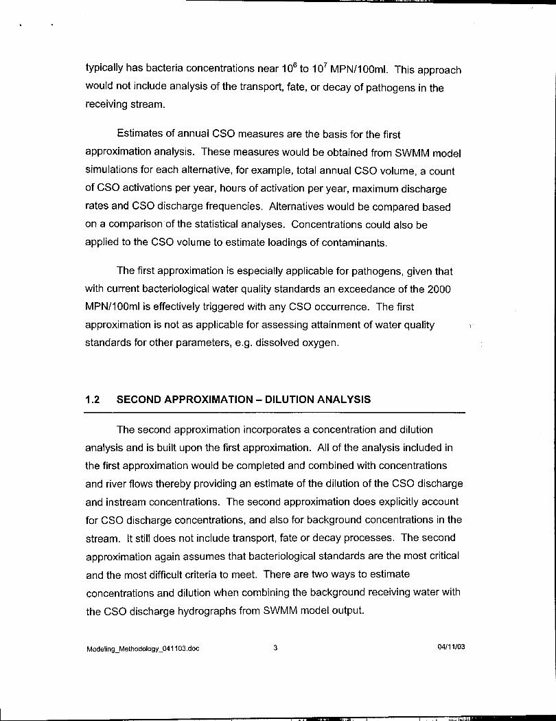
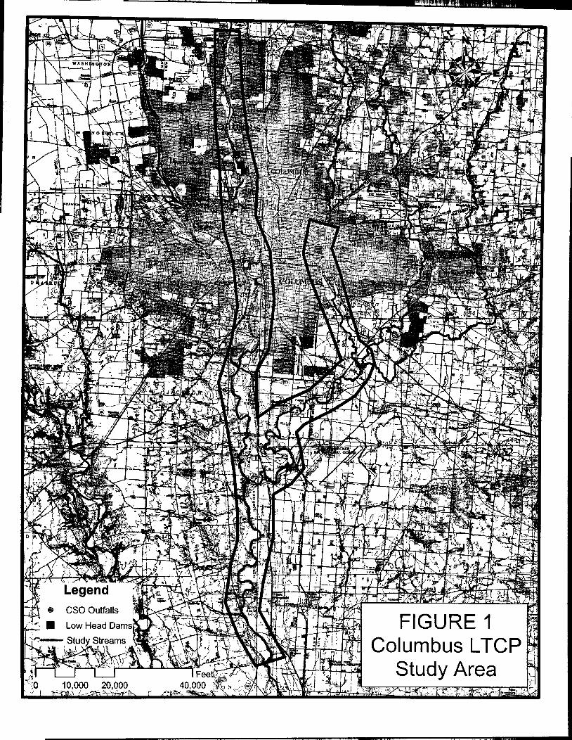
This paper focuses primarily on the City of Columbus's proposed L TCP

update. The City currently has CSO discharge points on Alum Creek, the

Olentangy River, and the Scioto River. FIGURE 1 (located at the end of this

document) shows the proposed study area along with the location of CSO

discharge points. One significant issue with the study area is the fact that there

are several dams within the study area and that the majority of CSO discharge

locations are upstream of these low-head dams. The most significant CSO

discharge is the Whittier Street Storm Stand-By Tanks, which is at the toe of

Greenlawn Dam, the most downstream dam on the Scioto River. FIGURE 1 also

shows the location of the dams relative to the CSO discharge points.

The City of Columbus currently has a comprehensive SWMM model for

evaluating the hydraulic characteristics of the sewage collection system including

the CSO areas of the City. The City also has a comprehensive QUAL2E water

quality model for evaluating steady-state water quality conditions in the receiving

waters within parts of the study area. The current QUAL2E model can evaluate

water quality conditions from Greenlawn Dam on the Scioto River to just

upstream of Circleville and from Livingston Avenue on Alum Creek to the mouth

of Big Walnut Creek on the Scioto River.

Modeling_Methodology_041103.doc 1 04/11/03

.

There are a number of analyses that could be completed to support the

demonstration or presumptive approach, i.e., project the attainment of water

quality standards and use designations, or quantify the impacts of a L TCP

alternative on a receiving water or reduce CSO discharges to 4 per year. There

are three approximation methods with special relevance to the City's goals; these

are briefly explained below and further explained in later sections.

A critical step in selecting appropriate receiving water modeling and

analysis techniques for L TCP development is identifying the water quality

parameters of primary interest. The screening and selection of analysis

techniques presented in this paper is predicated on the assumption that

pathogens are the controlling water quality parameter for the City's L TCP. This

assumption is based on the simple reality that in order to preclude CSOs from

violating current bacteriological standards, effective reduction of CSO discharge

for small storms (12-Month or less) is often the only option. With reduction of

CSOs to control pathogens, control of other water quality parameters in the CSO

discharge is obviously also aGcomplished. In this situation, sophisticated water

quality analysis of other parameters becomes unnecessary.

Disinfection is also a viable alternative for reducing pathogen levels in

CSO discharge. Facility requirements for disinfection make it a less feasible

alternative for some CSO discharge locations. Also, disinfection rather than

reduction of CSO discharge does not preclude the need for water quality analysis

for other parameters such as ammonia or dissolved oxygen. Effective

disinfection of CSO discharge can reduce pathogen concentrations to less thanthe water quality standard of 2000 MPN/100ml. .

1.1 FIRST APPROXIMATION -END OF PIPE ANALYSIS

A first approximation would involve an end of pipe analysis using output

from a continuous SWMM model simulation. The assumption with an end of pipe

analysis is that any CSO discharge would cause bacteria concentrations greater

than 2000 MPN/100ml at the end of the discharge pipe since CSO discharge


",'

..."."

.

typically has bacteria concentrations near 1 06 to 1 07 MPN/100ml. This approach

would not include analysis of the transport, fate, or decay of pathogens in the

receiving stream.

Estimates of annual CSO measures are the basis for the first

approximation analysis. These measures would be obtained from SWMM model

simulations for each alternative, for example, total annual CSO volume, a count

of CSO activations per year, hours of activation per year, maximum discharge

rates and CSO discharge frequencies. Alternatives would be compared based

on a comparison of the statistical analyses. Concentrations could also be

applied to the CSO volume to estimate loadings of contaminants.

The first approximation is especially applicable for pathogens, given that

with current bacteriological water quality standards an exceedance of the 2000

MPN/100ml is effectively triggered with any CSO occurrence. The first

approximation is not as applicable for assessing attainment of water quality ;

standards for other parameters, e.g. dissolved oxygen.

1.2 SECOND APPROXIMATION -DILUTION ANALYSIS

The second approximation incorporates a concentration and dilution

analysis and is built upon the first approximation. All of the analysis included in

the first approximation would be completed and combined with concentrations

and river flows thereby providing an estimate of the dilution of the CSO discharge

and instream concentrations. The second approximation does explicitly account

for CSO discharge concentrations, and also for background concentrations in the

stream. It still does not include transport, fate or decay processes. The second

approximation again assumes that bacteriological standards are the most critical

and the most difficult criteria to meet. There are two ways to estimate

concentrations and dilution when combining the background receiving water with

the CSO discharge hydrographs from SWMM model output.

ModelinQ_MethodoloQy_041103.doc 3 04111103

, ". "," ,,","cl,,"

""'" !ft

.

1.2.1 Spreadsheet Analysis

Spreadsheet analysis is the simplest form of the second approximation

approach. Using this approach would involve combining the probability of a

stream discharge rate with the predicted CSO discharge rates (from the SWMM

model). Event mean concentrations would be incorporated into the SWMM

model discharge rates to predict concentrations.

1.2.2 Monte Carlo Simulation

A Monte Carlo simulation is a more complex approach to the second

approximation. The Monte Carlo simulation would incorporate uncertainties in

the values of concentrations and flow rates. The results would be very similar to

the spreadsheet analysis.

1.3 THIRD APPROXIMATION -DILUTION/DECA Y ANALYSIS

The third approximation is the most complex and comprehensive analysis

that could be performed in support of the demonstration approach. A continuous

SWMM simulation similar to the analysis mentioned above would be used to

predict CSO discharge hydrographs as input for subsequent receiving water

analysis. This approach would account for the transport, fate and decay of the

parameters of interest. The choice of modeling tools depends on the specific

questions that need to be answered and how detailed the simulation needs to be

to obtain necessary information.

1.3.1 Spreadsheet Steady-State Analysis (Pathogen)

Analysis via spreadsheet is possible but not recommended. It would be

possible to build a spreadsheet model to estimate the transport and decay for

pathogens but other models already exist for performing the similar types of

analyses more efficiently.


--

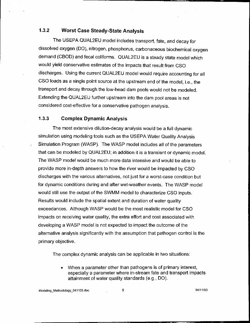
1.3.2 Worst Case Steady-State Analysis

The USEPA QUAL2EU model includes transport, fate, and decay for

dissolved oxygen (DO), nitrogen, phosphorus, carbonaceous biochemical oxygen

demand (CBOD) and fecal coliforms. QUAL2EU is a steady state model which

would yield conservative estimates of the impacts that result from CSO

discharges. Using the current QUAL2EU model would require accounting for all

CSO loads as a single point source at the upstream end of the model, i.e., the

transport and decay through the low-head dam pools would not be modeled.

Extending the QUAL2EU further upstream into the dam pool areas is not

considered cost-effective for a conservative pathogen analysis.

1.3.3 Complex Dynamic Analysis

The most extensive dilution-decay analysis would be a full dynamic

simulation using modeling tools such as the USEPA Water Quality Analysis

Simulation Program (WASP). The WASP model includes all of the parameters

that can be modeled by QUAL2EU; in addition it is a transient or dynamic model.

The WASP model would be much more data intensive and would be able to

provide more in-depth answers to how the river would be impacted by CSO

discharges with the various alternatives, not just for a worst-case condition but

for dynamic conditions during and after wet-weather events. The WASP model

would still use the output of the SWMM model to characterize CSO inputs.

Results would include the spatial extent and duration of water quality

exceedances. Although WASP would be the most realistic model for CSO

impacts on receiving water quality, the extra effort and cost associated with

developing a WASP model is not expected to impact the outcome of the

alternative analysis significantly with the assumption that pathogen control is the

primary objective.

The complex dynamic analysis can be applicable in two situations:

.When a parameter other than pathogens is of primary interest,especially a parameter where in-stream fate and transport impactsattainment of water quality standards (e.g., DO).


,

.When a permitee is considering the option of requesting a changein water quality standards as part of their wet-weather control plan.


.,..,

2.0 DATA REQUIREMENTS

Each of the relevant methods introduced in Section 1 above have certain

data requirements. These data requirements are summarized below, with

additional details on each of the data types provided in the subsequent

subsections.

The first approximation requires:

.SWMM model, which has already been developed. A time-intensive data collection effort for the SWMM model is notanticipated. Data collection would likely be limited to compilinghistorical rainfall data to develop an average, or typical,

precipitation year.

The second approximation requires:

.SWMM model.

.Compilation of streamflow records.

.Instream water quality.

.CSO discharge water quality

The third approximation requires:

.SWMM model.

.Compilation of streamflow records

.Instream water quality.

.CSO discharge water quality

.Worst-Case Steady State: QUAL2E model, which has alreadybeen developed. A time-intensive data collection effort for theQUAL2E model is not anticipated.

.Complex Dynamic: WASP model, which has not been developed.Additional water quality and hydrodynamic data would be requiredto develop the WASP model


,," cd- .

It should be noted that the City of Columbus has already suggested doing

a bacteria study for the CSO impacted streams, which would support the

instream water quality and CSO discharge water quality data needs.

2.1 HISTORICAL RAINFALL

Historical rainfall data analysis is necessary for the SWMM model. The

historical rainfall data will be analyzed to develop an average, or typical,

precipitation year. The analysis will include approximately 50 years of rainfall

data. The average rainfall year will be the baseline for all of the SWMM model

simulations, for both existing conditions and the alternative analysis.

2.2 HISTORICAL STREAM FLOW

Historical stream flow data would be necessary for performing dilution

models and dilution-decay models. Similar to rainfall, an average annual stream

flow would have to be developed for the receiving water. Further analysis that

compares streamflow to rainfall would better solidify the relationship or

correlation between the two datasets. A significant correlation may not exist, but

the goal would be to isolate an annual streamflow record that corresponds to the

average rainfall year.

2.3 INSTREAM WATER QUALITY (BACKGROUND CONDITIONS)

There are two main data types for instream water quality that are of

particular interest for modeling the impacts of CSOs on receiving streams -

pathogens and DO/CBOD/nutrients. For both of these data types, it is important

to characterize concentration not only in the impacted waters but also the

background concentrations. Furthermore, sampling of dry and wet weather

conditions is also necessary. The background conditions may on their own

exceed water quality standards with no CSO inputs. It is possible that many

pollutants typically associated with CSO discharges could also be originating

from other sources (wildlife, pets, fertilizer) during rain events.


The USEPA Combined Sewer Overflows Guidance For Monitorina and

Modeling, January 1999 notes that CSOs can affect several receiving water

quality parameters. It also states that the impact on one parameter is frequently

much greater than other parameters; therefore, relieving the impact by the one

parameter will likely relieve the other parameters. Pathogens are most likely the

highest impact considering current water quality standards and relieving

pathogen impacts through reduction of CSOs will most likely eliminate any DO,

CBOD and nutrient impacts.

2.3.1 Pathogens

As noted at the beginning of this section, the City of Columbus has

suggested a bacteria study to identify background levels and sources of bacteria.

2.3.2 Dissolved Oxygen, CBOD and Nutrients

DO, CBOD and nutrient data would be necessary for the transport, fate,

and decay modeling using QUAL2EU or WASP. The data would be used to

develop boundary conditions and calibration points for either model. The WASP

model would require the most extensive data collection effort.

2.4 CSO DISCHARGE WATER QUALITY

Sampling of CSO discharge is necessary to develop an understanding of

"typical" CSO discharge quality. The typical CSO discharge quality would be

applied to the SWMM CSO discharge results to estimate loadings. as part of the

existing condition assessment and alternatives analysis.

2.4.1 Pathogens

The collection of pathogen data for the CSO discharge points would be

included in the previously noted bacteria study. Sampling of CSO discharges

would need to begin during early activation and continue through the end of the

event. A full data set for a CSO discharge would allow the determination of an

event mean concentration.

Modelin9_Methodolo9y_041103.doc 9 04/11/03

" "",.u,

.

2.4.2 Dissolved Oxygen, CBOD, and Nutrients

Sampling procedures would be similar to the procedures for pathogens.

Sampling would need to begin at activation and continue at regular intervals

during the entire overflow event. Event mean concentrations would be

determined from the sampling data and applied to existing conditions and

alternatives analysis.

2.5 HYDRODYNAMIC DATA

The requisite hydrodynamic data already exist for Alum Creek and Big

Walnut Creek. In addition, the Ohio EPA developed hydraulic information for the

Scioto River south of the Greenlawn Dam. The US Corp of Engineers has a

well-developed HEC-RAS model for the Scioto River north of the Jackson Pike

WWTP. All of the existing data will be useful for evaluating CSO impacts on the

receiving waters with two possible exceptions.

The area of the Scioto River upstream of the Greenlawn Avenue Dam

would require additional hydrodynamic data if a WASP model is developed for

that area. Although there is an existing HEC-RAS model for the area upstream

of the Greenlawn Avenue Dam, it was developed for significantly higher flow

rates than what would be used for CSO impact modeling.

The Ohio EPA developed the hydraulic coefficients downstream of the

Greenlawn Avenue Dam in the early 1980's and Malcolm Pirnie revised some of

the coefficients between Greenlawn Dam and the JPWWTP in 2001. Given the

age of the hydraulic coefficients on the Scioto River, there may be a need to

update them as well for a CSO impact analysis. This would only need to be

completed if there is a significant lack of confidence in the dilution/decay model

results when run with wet weather flow rates.

2.5.1 Flow Monitoring

Flow monitoring at key locations along the Scioto River and Olentangy

River would be required for transport, fate, and decay modeling. The flow


monitoring would involve continuously recording level meters. Rating curves

would have to be developed for each flow monitoring point.

2.5.2 Cross Sections

Cross section data would be necessary for the areas upstream of the

Greenlawn Dam to develop hydrodynamic data for transport, fate, and decay

modeling.

2.5.3 Time of Travel

Time of travel data is extremely useful for developing hydrodynamic

models. If it is determined that dilution decay modeling must be completed in the

areas upstream of the Greenlawn Dam, then two separate time of travel studies

would be necessary. One study would need to be completed at a lower flow rate

and another at a higher flow rate. If time of travel work is completed for this

reach of the river, it would be advisable to extend the study south into Pickaway

County. Extending the study south would allow a more complete evaluation of

the existing hydraulic data for the $cioto River and could increase confidence in

current and future models.

11 04/11/03

Modeling_Methodology _041103.doc

",...,

..

3.0 FIRST APPROXIMATION ANALYSIS

The first approximation method analyzes the results of SWMM model

output and uses the model predictions of end-of-pipe CSO activity to compare

CSO abatement alternatives. The assumption for this analysis is that any CSO

discharge will cause an exceedance of 2000 MPN/100ml for pathogens

regardless of background concentrations. Also assuming the minimum sampling

frequency of five per month, two discharges in a 3D-day period could be an

exceedance of the primary contact water quality standard. Data requirements for

this analysis include historical rainfall data only. The current SWMM model used

by the City will be the primary tool for the analysis.

3.1 CONTINUOUS SWMM SIMULATIONS

The SWMM model will be used to simulate the sewer collection system for

the entire recreational season in which the bacteria use designation is applied.

The recreational season is May 1st to November 1st (6 months). It is possible to

extend the simulation to a full 12-month period, but this would require some

analysis of snowfall.

A representative annual rainfall pattern, or typical precipitation year, would

need to be developed as an input for the SWMM model. All of the rainfall data

available from a local or nearby National Weather Service station, typically more

than a 40 year record, will be analyzed. This analysis establishes average

annual measures and average monthly measures (e.g., total depth, number of

events, etc.) for the entire period of record. Using these definitions of average

characteristics, each year is reviewed to identify the real historical year that is the

closest to an average year. Once the closest real historical year is identified, the

distribution of rainfall events within that year and within individual months is

compared to the long-term average. Where necessary, individual events are

added, deleted, or traded to represent the long-term average distribution of

events. The final result is a synthetic, average annual rainfall record, developed

Modeling_Methodology _041103.doc 12 04/11/03

'. "".

'" ! )~I!

entirely from real historical data. This average annual rainfall has already been

developed by Columbus and will be the baseline for all SWMM continuous

simulations. The figure below is an example of an average annual rainfall record

developed for the Buffalo Sewer Authority SWMM model.

Avearge Annual Rainfall Hyetograph (hourly data)

i 1.20.cuc 1.00~

~ 0.80"-c~ 0.60

Date

3.2 SUMMARIZING ESTIMATED END-OF-PIPE MEASURES FROM THE

SWMM MODEL OUTPUT

The output of each SWMM model simulation will be processed and (

statistically summarized. The statistics for the end-of-pipe measures for each

alternative will be entered into a matrix for comparison.

The SWMM model output file will be processed using result-processing

tools developed by Malcolm Pirnie. These software programs extract the

information from SWMM output files and place them in readily usable Microsoft

Excel tables. The tools can then be used to begin summarizing the relevant end-

of-pipe results of each model simulation. The image below is an example of one

of the Malcolm Pirnie developed programs.


c, ..,,~., ..

"

,

00 Main File

O~ File ~o Append "out0 D DWF File " t.OU.

OO'lr PackKey File tviicrosoft Excel ":-:1"

0- w.iS Da~abi:)~e Microsoft Access

O~ Selection Text ASCII Text

08 EJror log ASCII Text

A number of relevant end-of-pipe results from SWMM model analyses are

listed in the following sections. The full performance of any single alternative

must be compared to other alternatives by an aggregate of these results. No

single summary such as number of activations would be an accurate assessment

by itself. For instance, there could be many activations per year but the

maximum flow rate, duration and volume may be low in comparison to other

alternatives. The system-wide summaries of all results will provide the best

snapshot of alternative performance.

3.2.1 Number of Activations

The L TCP guidance documents consider the number of activations a valid

measure of CSO performance for the demonstration and presumption

approaches. In fact, the presumptive approach is largely based on this metric. A

summary of the number of activations for each CSO can be developed from each

SWMM model simulation. The activation summary is developed on a CSO by

CSO basis; these results can then also be combined into a system-wide basis.

Different alternatives can be compared to determine if the number of activations

increases or decreases. As introduced previously J given the current

Modeling_Methodology _0411 03.doc 14 04/11/03

...1.., ."" ,."

"' ,

bacteriological water quality standard, estimates of the number of CSO

activations in a 3D-day period can serve as a surrogate for estimating the number

of water quality standard exceedances for bacteria assuming that disinfection or

treatment of CSO discharge is not employed.

3.2.2 Hours of Overflow

The duration or time extent from activation to zero flow of each CSO

discharge event is another valid measure of the performance of alternatives. The

total time of duration or sum of all events for each CSO can be computed. A

further evaluation would compute the frequency or cumulative frequency of

different durations for each CSO and/or the system. This frequency analysis

would answer questions such as what percent of the events exceeded a 1-hour

or 3-hour duration.

3.2.3 Total Overflow Volume

The volume of CSO discharge for each event is another important

measure of combined sewer system performance. Each rain event that causes

an overflow will produce a certain volume of discharge. The total volume of CSO

discharge for each alternative will be summarized for each CSO and on a

system-wide basis. Furthermore, the frequency or cumulative frequency of event

volume per CSO or for the system will permit a more in-depth understanding of

system behavior. Since volume can be directly converted to a load if

concentrations are applied, it is considered one of the most important measures

of combined sewer performance and receiving water impacts.

3.2.4 Maximum Flow

The maximum flow rate from any CSO will vary depending on the event

and the level of control. A frequency analysis of maximum flow rates for each

CSO will help assess the performance of the various alternatives.


",,~.., .., 'TO" W,""" "" '" C'W'"",

., '

3.2.5 CSO Flow Frequency

A CSO flow frequency analysis would be similar to the maximum flow

analysis but it would also include a time variable. The frequency of various flow

rates could be plotted for each CSO. For instance, a CSO could discharge at 1-

cfs for a total of 10 hours per year, 1.5-cfs for 5 hours per year and 2-cfs for 0.5

hours per year. The value of the y-axis would be hours and the x-axis would be

flow rate.

3.3 EXAMPLE CSO LTCP ALTERNATIVE ANALYSIS -USE OF

CONTINUOUS SIMULATION RESULTS

The following table is a partial list of CSO discharge points from a 3-month

continuous SWMM simulation presented for example purposes. The data is from

a Malcolm Pirnie project (2002) for the Buffalo Sewer Authority in Buffalo, NY.

The table shows the total duration of overflow (in hours) that the model predicted

for each CSO. The table also shows the number of activations or overflow

events. Events were defined using a 6-hour inter-event duration, i.e., an event

was considered a new event if the preceding 6 hours had zero flow.

cso 0 If II M d I N d M d I L ' k Duration of Number of

ua oeoe oernOrtl (h) Orflve ow r ve ows

001a WWTPOF WETWELLOF 22 9

003 5494 5500 103 8004 10208 10213 4 1004 10210 10221 4 1005 5868 5873 2 1006 5708 5710 468 10008 5904 5906 139 16010 5551 5553 26 8011 6728 6729 31 5012 6362 6363 31 10013 10034 10047 11 1014 9009 L9201 10 1015 15669 15670 8 1016 14964 14968 159 19016 BRO,OO SPP39w 5 2

017 14580 14584 385 14021 15439 L15434 6 1022 14690 L14678 34 3025 15467 15468 9 1

Modelin9_Methodolo9y_041103,doc 16 04/11/03

,---, ,...""" ","""" .."".,-,,~.,-

'0"' '""'1""",,"

March -May

CSO Model Outfall TotalOutfalilD Node ID Overflow Event Duration Frequency Distribution for CSO

Volume(cu. ft.) Outfall 010

001 WWTPGRIT 764,500,000001a WWTPOF 0 5 100.0%002 TBD TBD003 5494 993,500 ~ 4 80.0%

004 10208 & 10210 2,741,000 ; 3 60.0%005 5868 114,200 ~006 5708 109,800,000 i 2 -40.0%

""008 5904 642,800 u. 1 20.00A010 5551 898,800 °

011 6728 2,015,000 0 .0%

012 6362 2,220,000 "' f\, ~ ~ ~ ~ Co <0 ~ ~013 10034 1,961,000 '" "'_"O~0014 9009 1,666,000 ~.

015 15669 1,477,000 Duration in Hours016 14964 & BRO.OO 429,100017 14580 13,170,000 I_~p__,,---, --"""" I_~:..- °, I021 15439 79,630 I_Frequency ::!:Cumulative % I022 14690 824,600025 15467 362,700

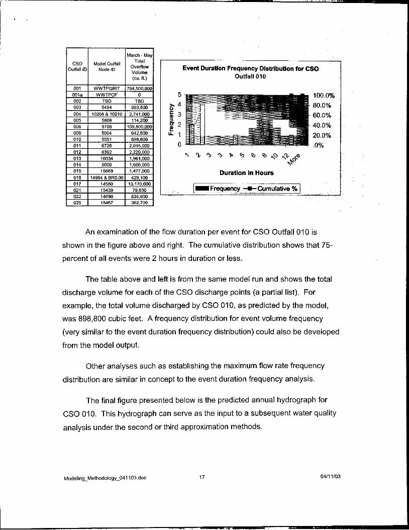
An examination of the flow duration per event for CSO Outfall 010 is

shown in the figure above and right. The cumulative distribution shows that 75-

percent of all events were 2 hours in duration or less.

The table above and left is from the same model run and shows the total

discharge volume for each of the CSO discharge points (a partial list). For

example, the total volume discharged by CSO 010, as predicted by the model,

was 898,800 cubic feet. A frequency distribution for event volume frequency

(very similar to the event duration frequency distribution) could also be developed

from the model output.

Other analyses such as establishing the maximum flow rate frequency

distribution are similar in concept to the event duration frequency analysis.

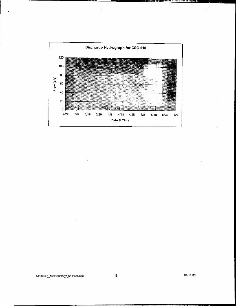
The final figure presented below is the predicted annual hydrograph for

CSO 010. This hydrograph can serve as the input to a subsequent water quality

analysis under the second or third approximation methods.

Modelin9_Methodolo9y_041103,doc 17 04/11/03

I" "'!,"II"!"' ",,'C

Discharge Hydrograph for CSO 010

120

100

80"Ui'...u~ 60

~E.u.

40

20

0

2/27 3/9 3/19 3/29 4/8 4/18 4/28 5/8 5/18 5/28 6/7

Date & Time


""" f

.-

4.0 SECOND APPROXIMATION ANALYSIS

The second approximation method will directly build upon the first

approximation by adding concentrations and stream flow to account for dilution

effects and to identify potential instream concentrations. This step is a natural

extension of the first approximation approach, although the answers will typically

be similar with respect to estimates of bacteriological water quality exceedances.

Adding dilution via background streamflow will reduce the duration of

exceedances at the beginning and tail end of each event because exceedances

will be based on a comparison of predicted instream concentrations to water

quality standards, rather than on CSO activations. The advantage of this

analysis would be the ability to predict instream concentrations of contaminants

at the discharge points (under the simplifying assumption of complete mixing)

including background concentrations.

4.1 SUMMARIZING ESTIMATED END-OF-PIPE MEASURES FROM THE

SWMM MODEL OUTPUT

The end-of-pipe analysis described in SECTION 3.0 will still be applicable

for the second approximation analysis. The significant additional step that would

be necessary for this analysis but unnecessary for the previous analysis is the

application of concentration to the CSO discharge. This requires a definition of

"typical" CSO discharge quality, as noted in SECTION 2.0. If CSO discharge

concentrations were not accounted for in the calculation, the only information that

could be determined from the dilution analysis is the percentage of river flow that

isCSO.


.""

4.2 STREAM FLOW PROBABILITY FOR THE DILUTION CALCULATION

The base streamflow for any CSO event can vary depending on the

season and preceding rain events. Because background flow varies, applying a

single background flow is not an entirely accurate method of estimating dilution.

As a simplifying assumption, the average monthly flow would be a reasonable

estimate. The figure below represents the average monthly streamflow for the

entire period of record at the JPWWTP USGS Gaging Station.

Average Flow of the Scloto River at the JPWWTP USGS Gaging Station

4000

3500

3000

..-2500~ui 20000

u: 1500

1000

500

01/1 2/1 3/3 4/3 5/4 6/4 7/5 8/5 9/5 10/6 11/6 12/7

Day of Year

-30-Day ~~ng Awrage .A\9 Daily Row

Using the average plus some standard deviation from the average to

predict in stream concentrations would be slightly more robust than just applying

the appropriate monthly average value. To extend beyond use of an average

streamflow (or band around the average), one would need to examine the

frequency distribution of the monthly streamflow and apply the probability of

stream flow rates to the dilution calculations. The figure below is a histogram of

the flow rate for the month of April. The end result of the analysis would be a


"'..,"

" w' , ,""'" '"1""1" , 11'~f'"

probability distribution of a particular concentration occurring in the stream for a

given CSO event.

Frequency Distribution of Scioto River Flow during the Monthof April from the JPWWTP USGS Gageing Station

100.00%90.00%

80.00%

>- 800 70.00%

g 60.00%~ 600 50.00%coe 400 40.00%LL 30.00%

200 20.00%

10.00%0 .00%

~~~~~~~~~~~~~~~ 0~~ ~~ ~~ A~~ ~~ ~~ ~~ ~~ ~~ ~~ ~~ ~~ ~~ ~~ ~~ -~o~'" i)j ~ \ OJ ,,'" "i)j ,,~ "'" "OJ C1,,'" C1"i)j ~ rr:: C1"OJ ~.

Flow (cfs)

-Frequency ~ Cumulative %

There is also some correlation between rainfall and stream flow. The

correlation of historical rainfall and streamflow datasets would need to be

analyzed and incorporated into the analysis. Incorporating the correlation would

better account for the probability of a concentration occurring in the stream for a

given CSO event. For example, during a very wet spring with significant volumes

of rainfall, the stream flow rate would most probably be higher than average. The

opposite would most probably be true during a dry or low rainfall volume spring.


""'.

"!" "'"" , "'If'W'!l

4.3 SPREADSHEET ANALYSIS FOR COMBINED PROBABILITY OF CSO

DISCHARGE AND STREAMFLOW

A spreadsheet analysis can be performed to provide a single value for the

probability of exceedance of a single instream concentration, for example 2000

most probable number per 100ml (MPN/100ml) bacteria. To obtain the single

value, the probability of background streamflow and concentration would be

combined with the probability of CSO flow rate and concentration.

The process of combining probabilities would be completed along the

length of the stream for each CSO encountered. For each new CSO

encountered, the background streamflow will have increasingly higher

concentrations of bacteria if the upstream CSO was also discharging. The

analysis would not include decay; therefore, travel time would be irrelevant. The

other possible approach is to sum all CSO discharges system wide and apply the

system wide flow and concentration probability (i.e. load) to the stream

background flow and concentration. The system wide approach would best be

applied at the downstream end of the CSO areas.

4.4 MONTE CARLO ANALYSIS TO COMBINE PROBABiliTIES OF CSO

DISCHARGE AND STREAMFLOW

A Monte Carlo analysis would be a more advanced approach as

compared to the dilution only model. A Monte Carlo analysis would use the

probability distributions of stream flow rates, instream concentrations, CSO flow

rates, and CSO concentrations as inputs to the dilution equation. The equation

would be solved 1000 or more times with each solution using a randomly

selected value from each probability distribution.

The Monte Carlo results would be presented as frequency or cumulative

frequency distributions of the resulting modeled set of instream concentrations.

Modelin9_Methodology_041103.doc 22 04/11/03

" "',"" "I"":

~

Determination of the percent of time that the instream concentration will exceed

any value can be easily extracted from the distribution.

4.5 EXAMPLE CSO L TCP ALTERNATIVE ANALYSIS -USE OF DILUTION

RESULTS

The results from the second approximation would be very similar to the

statistical summaries from the first approximation. For example, a histogram of

the duration of concentrations could be created that would be similar to the

histograms presented in SECTION 3. The difference would be that the

histograms and distributions would reflect predicted concentrations in the

receiving stream, as opposed to end-of-pipe CSO measures.

,-

23 04/11/03

Modelin9_Methodolo9y_041103.doc

.

""1!j!!I'f"'"

.

5.0 THIRD APPROXIMATION ANALYSIS

The third approximation method incorporates dilution, transport, fate, and

decay modeling using either a steady state or dynamic model. The dilution-

transport-fate-decay modeling is the only analysis that is capable of predicting

the complex interactions between multiple CSO contaminants such as ammonia

and CBOD impacts on dissolved oxygen. Again, it is important to recognize that

the impacts of bacteria will most likely dominate the analysis since it will be the

most difficult water quality criterion to meet. Identifying an alternative that meets

bacteria water quality standards through CSO reduction is expected to also meet

other water quality standards such as ammonia and instream DO levels.

5.1 USE OF ESTIMATED END-OF-PIPE MEASURES FROM THE SWMM

MODEL OUTPUT

The specific use of the SWMM model output in this third approximation

analysis depends on the choice of steady state or dynamic modeling. If steady

state modeling in QUAL2E is chosen, then the end-of-pipe summary statistics

determined in SECTION 3.2 above will be used as inputs for the QUAL2E model.

If dynamic modeling is used, then the full hydrograph output of the continuous

SWMM simulation will be used as the input to the dynamic WASP model. In

either case, an event mean concentration of the modeled parameters would have

to be combined with the SWMM model output to develop the appropriate load

inputs.

5.2 QUAL2E MODEL SIMULATION -WORST CASE STEADY STATE

QUAL2EU is a USEPA developed receiving water model capable of

predicting the steady-state transport, fate, and decay of DO, CBOD, nitrogen,

phosphorus, suspended algae, and fecal coliforms as well as three user defined

constituents. The City already has a well-developed QUAL2E model for the

Scioto River downstream of Greenlawn Dam and for Alum Creek and Big Walnut

Creek downstream of Livingston Avenue. The QUAL2E analysis can be used to


.., , ,,""V ""111~ fl!

.

examine the instream DO response and pathogen decay under steady-state flow

conditions. It is important to realize that the pathogen capability of QUAL2E is a

simple first order decay process and it is only affected by temperature.

Pathogens have no effect on, nor are they affected by, any other process in the

QUAL2E model.

For this application, the existing QUAL2E model would be run at low wet-

weather flow rates determined from historical streamflow data. The lower flow

rates are considered conservative and would reduce reaeration and travel time,

causing reduced pathogen transport and greater dissolved oxygen sags to occur

in the stream. The inputs at CSO discharge points are entered as boundary

conditions.

On the Scioto and Olentangy Rivers, all of the CSO discharge points

would be entered at the headwater of the existing model, which is Greenlawn

Dam. Greenlawn Dam is also the location of the most significant CSO on the

Scioto River, the Whittier Street Storm Tanks. Any CSO discharge points

downstream of the Greenlawn Dam would be input at the appropriate location.

There is only one CSO discharge point on the Alum Creek. The Alum

Creek Storm Tanks are approximately 31 DO-feet upstream of the current upper

boundary of the QUAL2E model of Alum and Big Walnut Creeks. The Alum

Creek Storm Tank would be input as part of the headwater condition of the

model.

The QUAL2E model is a conservative method of examining the stream

response for CSO L TCP development because all of the loadings will be entered

as constant, and at their maximum level, rather than time-varying. The USEPA

L TCP Modeling Guidance recognizes QUAL2E as a model valid for analyzing

receiving water impacts. Furthermore, the guidance documents note that

QUAL2E is conservative in this application and will provide worst-case

predictions. In other words, the instream concentrations would not be expected

to exceed the results predicted by the model. Different alternatives would be


.."

" ,-~-~.,.,-,._-

compared based on the results of the QUAL2E model. The longitudinal extent of

the impacts from CSO contaminants could also be identified from the QUAL2E

model, although the predicted longitudinal extent may be non-conservative given

the use of lower streamflow rates.

The current QUAL2E model will require validation with wet weather data.

The validation work is currently proposed to be completed.

5.2.1 QUAL2EU Uncertainty Analysis

The Monte Carlo analysis option of QUAL2EU could be invoked for a

more robust analysis of the receiving water quality impacts. The Monte Carlo

analysis would be very similar to the spreadsheet version of Monte Carlo

analysis in SECTION 4.4 except QUAL2EU has a built-in Monte Carlo tool. The

characteristics of all of the modeled constituents would have to be examined to

identify the best probability distribution and also the coefficient of variance

(standard deviation/mean). The Monte Carlo analysis results could be presented

in a frequency distribution or cumulative frequency distribution.

5.3 WASP MODEL SIMULATION -COMPLEX DYNAMIC ANALYSIS

WASP is another USEPA-developed model that can be used to model the

transport, fate, and decay of the same parameters as QUAL2E, along with many

more parameters. WASP is a dynamic model that can simulate time-varying

streamflow rates along with time varying loading sources such as CSOs, rather

than applying them as worst-case, steady-state sources. The WASP model

would be a more realistic representation of the river and CSO system under wet-

weather conditions.

The information on the physical configuration of the river reaches in the

current QUAL2E models could be used to develop the WASP models for those

reaches. Extending the WASP model upstream of the Greenlawn Dam would be

significantly more difficult and costly due to the required data collection effort.


" "".,0

'" !'~!!H'""""""~I"~!l'i!"'!!4'!r!"tJ!~!"!'I!!!~!i'

5.3.1 Coupling WASP with SWMM Model

The SWMM model output hydrographs would be used as a time-varying

input for the WASP model. Event mean concentrations would be applied to the

hydrograph thereby developing the appropriate loads for the modeled

parameters. The location of the CSO inputs incorporated in the model will

depend on the extent of the modeled network.

5.3.2 WASP Based on Existing QUAL2E Network

The representation of river reach characteristics and hydrodynamics in the

current QUAL2E model can be converted for use in WASP. The WASP model

would require calibration and validation to existing wet-weather flow and water

quality data and quite possibly some new wet-weather data.

5.3.3 WASP Based on Extended Network for Dam Pools

WASP (or more generally a dynamic model) is the only recommended

dilution, transport, fate, and decay model for the area upstream of Greenlawn

dam. The extensive pools created by the dams result in slow moving water and

applying constant CSO sources would be overly conservative. Using time-

varying CSO loading in the dam pools would be more appropriate. Extending the

model network upstream of Greenlawn Dam would allow the CSO inputs to be

located at their actual discharge points into the pools.

Extending the network upstream of Greenlawn Dam will require a

significant data collection effort to define the hydraulics in the dam pools. The

data collection effort was noted previously in SECTION 2.0. In particular, data

would need to include continuous flow monitoring at multiple sites, stage-

discharge curve development and time of travel studies.

5.3.4 Simulation of Conservative and Non-Conservative

Pollutants

WASP can readily model DO, CBOD, ammonia, nitrogen, phosphorus and

bacteria. Furthermore, WASP has the capability to model sediment processes,


,""' 11ri:!\!',""iC!"'""i"fll'I!',

.I

although sediment modeling adds a significant level of complexity to the model

and data collection effort. Bacteria are still the most likely contaminant to focus

on given the difficulty in meeting bacteriological water quality standards under

wet weather conditions.

The WASP model for either network will be run continuously for the same

time period as the SWMM model. The results of the WASP model are time-

varying instream concentrations for the modeled parameters. These results can

be presented as a cumulative frequency distribution of parameter concentrations,

and these distributions can be used to compare abatement alternatives. The

longitudinal extent of the water quality impacts resulting from CSO discharges

can also be reasonably predicted via the WASP model.

5.4 EXAMPLE CSO L TCP ANALYSIS -USE OF WASP MODEL OUTPUT

The following table presents an example of how continuous WASP model

output can be used to assess the impact of CSOs in terms of water quality

standards exceedances. These results are from a continuous 6-month

simulation using a calibrated WASP model of the Cuyahoga River. Several

points can be identified from the table.

.The table shows that the majority of the modeled river reachesviolated the Fecal Coliform Geometric Mean requirement of 1000coliform per 100ml for 2 months out of the 6-month recreationalperiod (see SECTION 7 for details on the water quality standardfor fecal coliforms).

.The 10-percent rule of the fecal coliform water quality standard, i.e.no more than 1 O-percent of the samples in a 30-day period canexceed 2000 coliform per 10ml, was exceeded every month by 35of the 38 discharge points. The remaining 3 discharge pointsexceeded the standard 5 months out of the 6-month simulation.

.The table shows that there were no exceedances of the DO.standard in the stream during the six-month period. This particular

result is in some ways unique to the project situation being used in

this example.

28 04/11/03

Modeling_Methodology_041103.doc

'""'"

, " ""'"' """i'!IF '! f t"!"I'f'PI"!!

.

I

The 1 a-percent rule observation highlights the concept that virtually any

CSO discharge will result in an exceedance of the bacteriological water quality

standard. The dynamic modeling used on the example project was necessary for

other parameters; however, it is very relevant to observe that in terms of bacteria,

the same conclusion regarding water quality exceedances could have been

achieved using the first approximation analysis. The first approximation would

have taken significantly less time and dollars to complete.

.-


,~ Ii'!! !r""",~,!",

.,

, TABLE 12-11.Summary of Water Quality Violations

Cuyahoga River .(Based on Predictions From the Water Quality Model for the SiX-Month Recreational Period (May-october) .

Number of MonthsNumber of Months (;hat the Fecal Number of Months

when the FecaI Coliform samples hi Vioiation of theColiform Geometric exceed 2000 cot per Primary Contact Number of Days fuMean is greater than 100 ml mor~ "than Bacteriological Violation of the DO1000 cot per..l00 ~l 10% of the time Standard Standard

0 00 00 00 00 00 ..0

0 00 0

0 .00 00 0O' 0

2 02 02 02 02 02 02 02 02 02 (- 02 02 0

CR(38'-3) 2 6 6 0CR(38-2) 2 6 6 0CR(38-1) 2 6 6 0CR(37-5) 2 6 6 0CR(37-4 2 ---6 6 0CRL(37-45) 2 6 6 0CR(37-30) 2 6 6 0CR(37~lO) 2 6 6 0CR(36-30 2 5 5 0CR(35-60 2 5 5 0CR(34-38 2 5 5 0CRL(42- 2 6 6 0CRL(44- 0 6 6 0CRL(45-42) 0 6 6 0


.,

.,. ,

6.0 PREVIOUS WORK

6.1 BUFFALO SEWER AUTHORITY, NEW YORK

Malcolm Pirnie is the Coordinating Consultant for the Buffalo Sewer

Authority's development of a CSO L TCP. As the Coordinating Consultant,

Malcolm Pirnie is leading a team of four consultants on the project, and is

responsible for model development, characterization of existing conditions, and

preparing data collection and alternative screening protocols for use by the other

three consultants working in their respective drainage areas (Districts).

BSA's 68 CSOs discharge into the Buffalo River, Black Rock Canal, and

Niagara River, along with several major urban streams that run through the City

of Buffalo. Early in the project, it was recognized that attainment of water quality

standards would be an imperfect measure for comparing CSO abatement

alternatives, given the significant background concentrations in BSA's receiving

waters. Therefore, sophisticated water quality modeling was not incorporated in

the project; rather, predicted end-of-pipe CSO measures were used to prioritize

CSOs under existing conditions, and provide a measure of benefit for abatement

alternatives. Sophisticated water quality modeling may still be pursued in local

sensitive areas, but only where its usefulness is demonstrable; its use as a

system-wide analysis tool was not warranted.

An example of the use of predicted end-of-pipe measures from continuous

XP-SWMM model simulations for the BSA project is shown below. This figure

shows predicted annual overflow volume by CSO, and can be used to quickly

identify the significant contributors in terms of annual CSO volume. From this

figure, it is clear that approximately 80 percent of the annual system-wide CSO

volume comes from the top ten CSOs.


"'" "rl"~ "~ lllr!"~io; l, ,"OJ'''''''''"

... .

Figure 5-2Cumulative percent of total 12 month overflow volume by CSO

1200%

..e~ 1(XJ.0% --

c>

~C 800%....~~ 0 =..'; ~ 600%

~ ..= ~=~.(~ 40.11'/.-~=";e~ 200'/.

U

00'1.~ .~~s;;~.e= 8~8. s~~"~ ."~§.f~ 0.' ~§~~ "~~, ~ § ~ ~.. §~~

CSO ID

6.2 CITY OF FORT WAYNE, INDIANA

The City of Fort Wayne, Indiana, submitted their draft CSO L TCP to the

'1ndiana Department of Environmental Management and USEPA in July of 2001.

The draft L TCP has been reviewed by USEPA, and the City is currently engaged

in comment response and negotiation.

A team of consultants led by Malcolm Pirnie developed the L TCP for the

City, including dynamic collection system and receiving water modeling tools.

The receiving water modeling tools were used to characterize CSO impacts

under existing conditions to a high level of detail, resulting in concentration

frequency distributions such as those shown below.


10 10

.-10 .-J -10E -J

0 E0 Q

-0~ , ~-0;10 -.0 ""4j10

:=' .2-""0 ~() 0

.()U;,0 .III .10

110 110 .

0.01 0.1 1 10 20 ..10 eo ".It 0.01 0.1 1 10 10 80 10 00 .".t Percent Less Than or EqUBI to a Given Value Percent Leu Than or Equal to a Given Value

Example Pathogen Frequency Distribution in a Fort Wayne Receiving Water Reach

Predicted end-of-pipe measures were used as the primary method to

characterize the benefit of improvement alternatives, with reductions in CSO

activations used as a surrogate for reduction in number of bacteriological water

quality exceedances.

6.3 CITY OF AKRON, OHIO

The City of Akron submitted their draft CSO L TCP to Ohio EPA in early

2000. They are currently in the final stages of negotiating the final L TCP with

Ohio EPA and USEPA.

Malcolm Pirnie was the modeling consultant on the City's L TCP

development team. Using XP-SWMM for the collection system, and WASP for

the receiving streams, a number of continuous annual simulations were

performed. Conclusions from the modeling of existing conditions were as

follows:

.Dissolved oxygen depression does occur during wet-weatherevents, but exceedances of DO water quality standards are rare.

.Exceedance of bacteriological water quality standards occursregularly during wet weather, due to both upstream concentrations

and CSO discharges.


, ,""j~"'~I!'"

"

Given these conclusions, widespread use of the water quality modeling tools to

assess the benefit of alternatives in terms of attainment of water quality

standards was not warranted, since attainment would not be sensitive to CSO

control levels to to background concentrations. Rather, reduction in end-of-pipe

measures was used as the primary measure of benefit for assessment of

abatement alternatives. This approach allowed the team to identify a "knee-of-

the-curve" control point for each CSO, where the incremental increase in benefit

(as measured by reduction in end-of-pipe activity) starts decreasing with increase

in control level. An example of this level of control relationship is shown below.

Regulator KO6285Comparison of Annual Number of Overflow Events

70

60

In 50CGI> 40w~~ 30GI>0 20

10

00 2 4 6 8 10 12 14

Design Storm Control Level (Months)

,. Storage Basins. Treatment Basins .I

04/11/03 Modeling_Methodology_O41103.doc 34

" ., ~ I

.~.

7.0 PATHOGEN MODELING

Throughout this paper, pathogens have been identified as the single most

difficult water quality parameter of concern with the City's CSO discharges. The

basis of this concern includes the current water quality standards for pathogens,

the average concentration of pathogens in CSO discharge, and previous L TCP

development experience.

The current water quality standard for pathogens is as follows:

Primary contact pathogen standard for Ohio requires that one of the two

following bacteriological standards are met:

Fecal coliform -geometric mean fecal coliform content (either MPN or

MF), based on not less than five samples within a thirty-day period,

shall not exceed 1,000 per 100 ml and fecal coliform content (either

MPN or MF) shall not exceed 2,000 per 100 ml in more than ten per

cent of the samples taken during any thirty-day period.

E. coli -geometric mean E. coli content (either MPN or MF), based on not

less than five samples within a thirty-day period, shall not exceed

126 per 100 ml and E. coli content (either MPN or MF) shall not

exceed 298 per 100 ml in more than ten per cent of the samples

taken during any thirty-day period.

Typical total coliform concentrations for CSOs are reported as 105 to 107

MPN/100ml. With these discharge concentrations, the volume of dilution water

alone would have to be at least 3 orders of magnitude greater than the CSO

volume. For instance, if the CSO discharge rate were 10 cfs and bacteria

concentrations were 107 MPN/1 OOml, then the stream would have to be flowing

at 50,000 cfs and have zero background coliform concentrations. This would

meet the 2,000 MPN/100mllimit. To put 50,000 cfs into perspective, a 500-year

flood on the Olentangy River is 28,700 cfs. The 1 a-year and 50-year floods at


'",..,

.~ .

the USGS gaging station located at JPWWTP on the Scioto River are 37,000 cfs

and 60,400 cfs respectively. According to 10-State Standards, a wastewater

treatment plant can cease operations past 25-year flood events.

In addition, the current bacteriological standard does not explicitly allow for

dilution to be accounted for in assessing attainment. Because there is no

guidance on when or where samples are to be taken, the standard creates the

possibility that a sample could be taken at a location where the effect of dilution

or mixing has not been achieved. Because of this, the standard might be

interpreted to effectively require that the concentration limits be met at all times,

at all locations, in the receiving stream.

7.1 FIRST APPROXIMATION SUFFICIENT FOR CURRENT PRIMARY

CONTACT USE DESIGNATION STANDARDS

For the reasons stated above, the first approximation analysis (summary

analysis of end-of-pipe estimates from continuous SWMM model simulation) is

considered a valid measure of existing conditions and abatement alternative

performance. Any CSO discharge will most likely cause an exceedance of the

current primary contact standard for bacteria, so the "measure" of exceedance

for the purposes of the analysis is a predicted CSO activation.

7.2 ADV ANT AGES/DISADV ANT AGES OF FIRST APPROXIMATION

The first approximation analysis for evaluating the L TCP alternatives has

the following advantages:

.Rapid Analysis of Pathogen Impacts.Significant Cost Savings.Does Not Require an Extensive Data Collection Effort.Readily Available Tools.Does Not Require Instream Background Concentrations.Attainment of Pathogen Criteria Through CSO Reduction will most

likely result in Attainment of other Water Quality Criteria

The disadvantages of the first approximation analysis are as follows:


.,'.,cO' 0/ 'ff1~!

, ., }

.Does Not Identify Instream Concentrations of Pathogens

.Omits Dilution, Transport, Fate, and Decay (Duration andLongitudinal Extent of Exceedance is Not Determined)

.Does Not Allow for Analysis of Parameters With SignificantInstream Fate and Transport Characteristics (e.g., CBOD/DO).

.Does Not Support Discussion of Modifying Water QualityStandards.

37 04/11/03Modeling_Methodology_041103.doc

..

..", """""

..' ,

8.0 CITY OF COLUMBUS RECOMMENDATION

There are many ways to approach the evaluation of CSO impacts on

receiving waters as part of a CSO L TCP development process. Obviously,

conducting the full suite of evaluations is typically not feasible due to cost and

schedule considerations. More importantly, complex analyses will most likely not

result in significant differences in the outcome of the CSO L TCP recommended

alternative, given that the controlling factor is typically the requirement to attain

current water quality standards for pathogens

8.1 SELECTING CRITERIA OF INTEREST

The first major step to determining an acceptable modeling and analysis

approach is to determine the criteria of interest. The single most difficult water

quality standard to attain is that for pathogens; therefore, it is the recommended

focus for the City's L TCP analysis. Ammonia toxicity and dissolved oxygen

depletion are also parameters of concern with CSO contaminants, but it is

anticipated that they will not be an issue if the water quality standards for bacteria

are attained through CSO reduction. If technology such as disinfection is used at

any CSO discharge point, it may be necessary to consider other parameters.

8.2 RECOMMENDED MODELING APPROACH

8.2.1 Pathogens and Second Approximation

The recommended primary modeling approach for the CSO L TCP is to

use the second approximation analysis as outlined in SECTION 4.0. The second

approximation approach can be applied to the CSO discharge points on the

Olentangy River, the Scioto River, and the Alum Creek. This includes the

analysis of the dam pools, which have significantly different hydraulics than the

areas on the Alum Creek and the Scioto River downstream of Greenlawn Dam.

Additional types of modeling in the dam pools would require significant data

collection efforts to define the hydraulics of the pools, with potentially no


"'

,. , , """ II~'II"

.rl ,,'

additional benefit to analyzing and comparing alternatives in terms of attainment

of bacteriological water quality standards.

8.2.2 Detailed Dilution Decay Modeling

If analysis of the CSO impacts for parameters such as DO and ammonia

is required, an analysis can be effectively conducted using the existing QUAL2E

models. Analysis of DO, ammonia and CBOD would be necessary if there is still

a significant discharge volume at any CSO location but the discharge is

disinfected. SECTION 5 covers the QUAL2E modeling in more detail. The

USEPA L TCP Guidance documents support QUAL2E and note that it can be

used in this manner, with the understanding that the results will represent worst-

case conditions.

8.3 PRESENTATION OF RESULTS

8.3.1 Summary Statistics of Exceedances

The results of the second approximation analysis would primarily be

summary statistics of in stream concentrations based on the SWMM model

output and historical streamflow. The output can be processed into frequency

distributions that would allow the likelihood of exceedance of bacteriological

water quality standards to be determined. The L TCP alternatives would be

compared based on the statistical evaluation.


"'"~!!! ,! I'

CSOOutfalis FIGURE 1

Columbus L TCP

Study Area

Documents

City of Columbus LONG-TERM CONTROL PLAN UPDATE … · RECEIVING WATER MODELING METHODOLOGY MEMORANDUM ... dissolved oxygen (DO), nitrogen, phosphorus, carbonaceous biochemical oxygen