Embed Size (px)
Citation preview

Cities in Bad Shape: Urban Geometry in India∗
Maria�avia Harari†
December 2016
Abstract
The spatial layout of cities is an important feature of urban form, previously highlighted by
urban planners but overlooked by economists. This paper investigates the economic implications
of urban geometry in the context of India. I retrieve the geometric properties of urban footprints
in India over time by combining a satellite-derived dataset of night-time lights with historic maps.
I then propose an instrument for urban shape that combines geography with a mechanical model
for city expansion: in essence, cities are predicted to expand in circles of increasing sizes, and
actual city shape is predicted by obstacles within each circle. With this instrument in hand,
I investigate how city shape a�ects the location choices of consumers and �rms, in a spatial
equilibrium framework à la Roback-Rosen. Cities with more compact shapes are characterized
by larger population, lower wages, and higher housing rents, consistent with compact shape being
a consumption amenity. The implied welfare cost of deteriorating city shape is estimated to be
sizeable. I also attempt to shed light on policy responses to deteriorating shape. The adverse
e�ects of unfavorable topography appear to be exacerbated by building height restrictions, and
mitigated by road infrastructure.
∗I am grateful to Jan Brueckner, Nathaniel Baum-Snow, Alain Bertaud, Dave Donaldson, Denise Di Pasquale,Esther Du�o, Gilles Duranton, Michael Greenstone, Melanie Morten, Daniel Murphy, Paul Novosad, Bimal Patel,Ben Olken, Champaka Rajagopal, Otis Reid, Albert Saiz, Chris Small, Kala Sridhar, Matthew Turner, Maisy Wongand seminar participants at MIT, NEUDC, UIUC, Columbia SIPA, LSE, Zürich, Wharton, the World Bank, Carey,the Minneapolis FED, the IGC Cities Program, the NBER Summer Institute, the Meeting of the Urban EconomicsAssociation, NYU, the Cities, Trade and Regional Development conference at the University of Toronto, CEMFI,UPF, Stockholm School of Economics, Stockholm University, the IEB Urban Economics Conference, the BarcelonaSummer Forum, PSU and the Central European Univeristy for helpful comments and discussions.†The Wharton School, University of Pennsylvania. [email protected]

1 Introduction
In urban economics we often o�er stylized representations of cities that are circular. Real-world
cities, however, often depart signi�cantly from this assumption. Geographic or regulatory con-
straints prevent cities from expanding radially in all directions and can result in asymmetric or
fragmented development patterns. While the economics literature has devoted very little attention
to this particular feature of urban form, city shape is an important determinant of intra-urban
commuting e�ciency: all else equal, a city with a more compact geometry will be characterized by
shorter potential within-city trips and more cost-e�ective transport networks, which, in turn, have
the potential to a�ect productivity and welfare (Bertaud, 2004; Cervero, 2001). This is particularly
relevant for cities in the developing world, where most inhabitants cannot a�ord individual means
of transportation (Bertaud, 2004). Cities in developing countries currently host 1.9 billion residents
(around 74% of the world's urban population), and this �gure is projected to rise to 4 billion by
2030 (UN, 2015).
This paper investigates empirically the causal economic impact of urban geometry in the context
of India, exploiting plausibly exogenous variation in city shape driven by geographic barriers. More
speci�cally, I examine how consumers and �rms are a�ected by urban geometry in their location
choices across cities, and in particular, how much they value urban shapes conducive to shorter
within-city trips. I investigate this in the framework of spatial equilibrium across cities à la Roback-
Rosen. By examining the impact of city shape on population, wages, and housing rents, I attempt
to quantify the loss from deteriorating geometry in a revealed preference setting.
As the country with the world's second largest urban population (UN, 2015), India represents
a relevant setting for researching urban expansion. However, systematic data on Indian cities and
their spatial structures is not readily available. In order to investigate these issues empirically, I
assemble a panel dataset that covers over 450 Indian cities and includes detailed information on each
city's spatial properties and micro-geography, as well as economic outcomes from the Census and
other data sources. I trace the footprints of Indian cities at di�erent points in time by combining
newly geo-referenced historic maps (1950) with satellite imagery of night-time lights (1992-2010).
The latter approach overcomes the lack of high-frequency land use data. For each city-year, I
then compute quantitative indicators for urban geometry, used in urban planning as proxies for the
patterns of within-city trips. Essentially, these indicators measure the extent to which the shape of
a polygon departs from that of a circle, higher values indicating a less compact urban footprint and
longer within-city distances. One of the contributions of this paper thus relates to the measurement
of the properties of urban footprints over time.
A second contribution of the paper concerns the identi�cation strategy. Estimating the causal
impact of city shape on economic outcomes is challenging, given that the spatial structure of a city
at a given point in time is in itself an equilibrium outcome. Urban shape is determined by the inter-
actions of geography, city growth and policy choices, such as land use regulations and infrastructural
investment. In order to overcome this endogeneity problem, I propose a novel instrument for urban
geometry that combines geography with a mechanical model for city expansion. The underlying
1

idea is that, as cities expand in space over time, they face di�erent geographic constraints - steep
terrain or water bodies (Saiz, 2010) - leading to departures from an ideal circular expansion path.
The relative position in space of such constraints allows for a more or less compact development
pattern, and the instrument captures this variation.
The construction of my instrument requires two steps. First, I use a mechanical model for city
expansion to predict the area that a city should occupy in a given year; in its simplest version, such
a model postulates a common growth rate for all cities. Second, I consider the largest contiguous set
of developable land pixels within this predicted radius; these pixels together form a polygon that I
denote as "potential footprint". I compute the geometric properties of the "potential footprint" and
I then proceed to instrument the geometric properties of the actual city footprint in that given year
with the shape properties of the potential footprint. The resulting instrument varies at the city-year
level, allowing me to control for time-invariant city characteristics through city �xed e�ects. The
identi�cation of the impact of shape thus relies on changes in shape that a given city undergoes
over time, as a result of hitting geographic obstacles. This instrument's explanatory power is not
limited to extremely constrained topographies (e.g., coastal or mountainous cities) in my sample.
With this instrument in hand, I document that city shape, a previously overlooked feature of
urban form, can have substantial economic implications. I �rst investigate whether households
and �rms value compact city shape when making location choices across cities. Guided by a simple
model of spatial equilibrium across cities, I examine the aggregate responses of population, wages and
housing rents, measured at the city level, to changes in shape. My �ndings suggest that consumers
value city compactness as a �consumption amenity�. All else equal, more compact cities experience
faster population growth. There is also evidence that consumers are paying a premium for living in
more compact cities, in terms of lower wages and, possibly, higher housing rents. Households locating
in non-compact cities require a substantial compensation: a one-standard deviation deterioration in
city shape, corresponding to a 720 meter increase in the average within-city round-trip distance,1
entails a loss equivalent to a 4% decrease in income. On the other hand, �rms do not appear to
require such a compensation: in equilibrium, compactness has negligible impacts on the productivity
of �rms. Thus, compact city shape can be likened to a pure �consumption amenity�, but not to
a �production amenity�. This does not automatically indicate that city compactness is ex-ante
irrelevant for �rms. These results indicate that, in equilibrium, �rms are able to optimize against
�bad� shape, in a way that consumers cannot. The margin through which �rms are able to neutralize
the e�ects of bad shape could be their location patterns within cities. Evidence from the street
addresses of �rms suggests that �rms located in non-compact cities tend to cluster in few employment
sub-centers. It is then consumers who have to bear the costs of longer commutes to work, and who
require a compensation for these longer trips through wages and rents.
In the second part of the paper I consider the role of policy: if city shape indeed has welfare
implications, what are possible policy responses to deteriorating shape? On the one hand, I consider
1As a reference, the average city in my sample has an area of 62.6 square km, and an average, one-way within-citytrip of 3.3 km.
2

infrastructural investment as a policy tool to counteract the e�ects of poor geometry. I �nd that
the negative e�ects of deteriorating geometry on population are mitigated by road infrastructure,
supporting the interpretation that intra-urban commuting is the primary channel through which
non-compact shape a�ects consumers. On the other hand, I consider land use regulations as a
co-determinant of city shape. I �nd that more permissive vertical limits, in the form of higher Floor
Area Ratios (FARs), result in cities that are less spread out in space and more compact than their
topographies would predict.
The remainder of the paper is organized as follows. Section 2 provides some background on
urbanization in India and reviews the existing literature. Section 3 documents my data sources and
describes the geometric indicators I employ. Section 4 outlines the conceptual framework. Section
5 presents my empirical strategy and describes in detail how my instrument is constructed. The
empirical evidence is presented in the following two sections. Section 6 discusses my main results,
which pertain to the implications of city shape for the spatial equilibrium across cities. Section 7
provides results on responses to city shape, including interactions between topography and policy.
Section 8 concludes and discusses indications for future work.
2 Background and previous literature
India represents a promising setting to study urban spatial structures for a number of reasons.
First, as most developing countries, India is experiencing fast urban growth. According to the 2011
Census, the urban population amounts to 377 million, increasing from 285 million in 2001 and 217
million in 1991, representing between 25 and 31 percent of the total population. Although the
pace of urbanization is slower than in other Asian countries, it is accelerating, and it is predicted
that another 250 million will join the urban ranks by 2030 (Mc Kinsey, 2010). This growth in
population has been accompanied by a signi�cant physical expansion of urban footprints, typically
beyond urban administrative boundaries (Indian Institute of Human Settlements, 2013; World Bank,
2013). This setting thus provides a unique opportunity to observe the shapes of cities as they evolve
and expand over time.
Secondly, unlike most other developing countries, India has a large number of growing cities.
This provides me with enough power for an econometric approach based on a city-year panel.
The challenges posed by rapid urban expansion on urban form and mobility have been gaining
increasing importance in India's policy debate, which makes it particularly relevant to investigate
these matters from an economics perspective. Limited urban mobility and lengthy commutes are
often cited among the perceived harms of rapid urbanization (e.g., Mitric and Chatterton, 2005;
World Bank, 2013), and providing e�ective urban public transit systems has been consistently
identi�ed as a key policy recommendation for the near future (Mc Kinsey, 2013). There is also
a growing concern that existing land use regulations might directly or indirectly contribute to
distorting urban form (World Bank, 2013, Sridhar, 2010, Glaeser, 2011). In particular, sprawl
has been linked to vertical limits in the form of restrictive Floor Area Ratios (Bertaud, 2002a;
3

Bertaud and Brueckner, 2005; Brueckner and Sridhar, 2012; Glaeser, 2011; Sridhar, 2010; World
Bank, 2013). Another example is given by the Urban Land Ceiling and Regulation Act, which has
been claimed to hinder intra-urban land consolidation and restrict the supply of land available for
development within cities (Sridhar, 2010).
Literature directly related to the geometric layout of cities is scant, but a number of literature
strands are tangentially connected to this theme.
The economics literature on urban spatial structures has mostly focused on the determinants
of city size and of the population density gradient, typically assuming that cities are circular or
radially symmetric (see Anas et al., 1998, for a review). The implications of city geometry are left
mostly unexplored. A large body of empirical literature investigates urban sprawl (see Glaeser and
Kahn, 2004), typically in the US context, suggesting longer commutes as one of its potential costs
(Bajari and Kahn, 2004). Although some studies identify sprawl with non-contiguous development
(Burch�eld et al., 2006), which is somewhat related to the notion of "compactness" that I investigate,
in most analyses the focus is on decentralization and density, neglecting di�erences in city geometry.
I focus on a di�erent set of spatial properties of urban footprints: conditional on the overall amount
of land used, I look at geometric properties aimed at proxying the pattern of within-city trips, and
view density as an outcome variable.2
The geometry of cities has attracted the attention of the quantitative geography and urban
planning literature, from which I borrow indicators of city shape (Angel et al., 2009). Urban
planners emphasize the link between city shape, average intra-urban trip length and accessibility,
claiming that contiguous, compact and predominantly monocentric urban morphologies are more
favorable to transit (Bertaud, 2004; Cervero, 2001). Descriptive analyses of the morphology of cities
and their dynamics have been carried out in the urban geography literature (see Batty, 2008, for a
review), which views city structure as the outcome of fractal processes and emphasizes the scaling
properties of cities.
In terms of methodology, my work is related to that of Burch�eld et al. (2006), who also employ
remotely sensed data to track urban areas over time. More speci�cally, they analyze changes in
the extent of sprawl in US cities between 1992 and 1996. The data I employ comes mostly from
night-time, as opposed to day-time, imagery, and covers a longer time span (1992-2010). Saiz (2010)
also looks at geographic constraints to city expansion, by computing the amount of developable land
within 50 km radii from US city centers and relating it to the elasticity of housing supply. I use the
same notion of geographic constraints, but I employ them in a novel way to construct a time-varying
instrument for city shape.
This paper also contributes to a growing literature on road infrastructure and urban growth in
developing countries (Baum-Snow and Turner, 2012; Baum-Snow et al., 2013; Morten and Oliveira,
2In this respect, my work is also related to that of Bento et al. (2005), who incorporate a measure of city shape intheir investigation of the link between urban form and travel demand in a cross-section of US cities. Di�erently fromtheir approach, I rely on a panel of cities and I attempt to address the endogeneity of city shape in an instrumentalvariables framework.
4

2014; Storeygard, 2016). Di�erently from these studies, I do not look at the impact of roads
connecting cities, but instead focus on trips within cities, as driven by urban geometry.
Finally, the geometry of land parcels in a rural, as opposed to urban context, has received some
attention in the law and economics literature. Libecap and Luek (2011) have explored the economic
implications of di�erent land demarcation regimes, showing that land values are higher when the
system in place generates regular-shaped parcels.
3 Data Sources
My empirical analysis is based on a newly assembled, unbalanced panel of city-year data, covering
all Indian cities for which a footprint could be retrieved based on the methodology explained below.
For each city-year in the panel, I collect data on the geometric properties of the footprint, the city's
topography, and various economic aggregate outcomes - in particular, population, average wages
and average housing rents.
3.1 Urban Footprints
The �rst step in constructing my dataset is to trace the footprints of Indian cities at di�erent points
in time and measure their geometric properties. The boundaries of urban footprints are retrieved
from two sources. The �rst is the U.S. Army India and Pakistan Topographic Maps (U.S. Army Map
Service, ca. 1950), a series of detailed maps covering the entire Indian subcontinent at a 1:250,000
scale. These maps consist of individual topographic sheets, such as that displayed in Figure 1A.
I geo-referenced each of these sheets and manually traced the reported perimeter of urban areas,
which are clearly demarcated (Figure 1B).
The second source is derived from the DMSP/OLS Night-time Lights dataset. This dataset is
based on night-time imagery recorded by satellites from the U.S. Air Force Defense Meteorological
Satellite Program (DMSP) and reports the recorded intensity of Earth-based lights, measured by
a six-bit number (ranging from 0 to 63). This data is reported for every year between 1992 and
2010, with a resolution of 30 arc-seconds (approximately 1 square km). Night-time lights have been
employed in economics typically for purposes other than urban mapping (V. Henderson et al., 2012).
However, the use of the DMSP-OLS dataset for delineating urban areas is quite common in urban
remote sensing (M. Henderson et al., 2003; C. Small et al., 2005; C. Small et al., 2013). The basic
methodology is the following: �rst, I overlap the night-time lights imagery with a point shape�le
with the coordinates of Indian settlement points, taken from the Global Rural-Urban Mapping
Project (GRUMP) Settlement Points dataset (Balk et al., 2006; CIESIN et al., 2011). I then set
a luminosity threshold (35 in my baseline approach, as explained below) and consider spatially
contiguous lighted areas surrounding the city coordinates with luminosity above that threshold.
This approach, illustrated in Figure 2, can be replicated for every year covered by the DMSP/OLS
dataset.
5

The choice of luminosity threshold results in a more or less restrictive de�nition of urban areas,
which will appear larger for lower thresholds.3 To choose luminosity thresholds appropriate for
India, I overlap the 2010 night-time lights imagery with available Google Earth imagery. I �nd that
a luminosity threshold of 35 generates the most plausible mapping for those cities covered by both
sources.4 In my full panel (including years 1950 and 1992-2010), the average city footprint occupies
an area of approximately 63 square km.5
Using night-time lights as opposed to alternative satellite-based products, in particular day-time
imagery, is motivated by a number of advantages. Unlike products such as aerial photographs or
high-resolution imagery, night-time lights cover systematically the entire Indian subcontinent, and
not only a selected number of cities. Moreover, they are one of the few sources that allow us to
detect changes in urban areas over time, due to their yearly temporal frequency. Finally, unlike
multi-spectral satellite imagery, night-time lights do not require any sophisticated manual pre-
processing and cross-validation using alternative sources.6 It is well known that urban maps based
on night-time lights will tend to in�ate urban boundaries, due to "blooming" e�ects (C. Small et al.,
2005).7 This can only partially be limited by setting high luminosity thresholds. In my panel, urban
footprints as reported for years 1992-2010 thus re�ect a broad de�nition of urban agglomeration,
which typically goes beyond the current administrative boundaries. This contrasts with urban
boundaries reported in the US Army maps, which seem to re�ect a more restrictive de�nition of
urban areas (although no speci�c documentation is available). Throughout my analysis, I include
year �xed e�ects, which amongst other things control for these di�erences in data sources, as well
as for di�erent calibrations of the night-time lights satellites.
By combining the US Army maps (1950s) with yearly maps obtained from the night-time lights
dataset (1992-2010), I thus assemble an unbalanced panel of urban footprints.8 The criteria for being
included in the analysis is to appear as a contiguous lighted shape in the night-time lights dataset.
3Determining where to place the boundary between urban and rural areas always entails some degree of arbi-trariness, and in the urban remote sensing literature there is no clear consensus on how to set such threshold. Itis nevertheless recommended to validate the chosen threshold by comparing the DMSP/OLS-based urban mappingwith alternative sources, such as high-resolution day-time imagery, which in the case of India is available only for asmall subset of city-years.
4For years covered by both sources (1990, 1995, 2000), my maps also appear consistent with those from theGRUMP - Urban Extents Grid dataset, which combines night-time lights with administrative and Census data toproduce global urban maps (CIESIN et al., 2011; Balk et al., 2006).
5My results are robust to using alternative luminosity thresholds between 20 and 40. Results are available uponrequest.
6An extensive portion of the urban remote sensing literature compares the accuracy of this approach in mappingurban areas with that attainable with alternative satellite-based products, in particular day-time imagery (e.g., M.Henderson et al., 2003; C. Small et al., 2005). This cross-validation exercise has been carried out also speci�cally inthe context of India by Joshi et al. (2011) and Roychowdhury et al. (2009). The conclusion of these studies is thatnone of these sources is error-free, and that there is no strong case for preferring day-time over night-time satelliteimagery if aerial photographs are not systematically available for the area to be mapped.
7DMSP-OLS night-time imagery overestimates the actual extent of lit area on the ground, due to a combinationof coarse spatial resolution, overlap between pixels, and minor geolocation errors (C. Small et al., 2005).
8The resulting panel dataset is unbalanced for two reasons: �rst, some settlements become large enough to bedetectable only later in the panel; second, some settlements appear as individual cities for some years in the panel,and then become part of larger urban agglomerations in later years. The number of cities in the panel ranges from352 to 457, depending on the year considered.
6

This appears to leave out only very small settlements. Throughout my analysis, I instrument all
the geometric properties of urban footprints, including both area and shape. This IV approach
addresses issues of measurement error, which could a�ect my data sources - for instance due to the
well-known correlation between income and luminosity.
3.2 Shape Metrics
The indicators of city shape that I employ (Angel et al., 2009a, 2009b),9 are used in landscape
ecology and urban studies as proxies for the length within-city trips and infer travel costs. They
are based on the distribution of points around the polygon's centroid10 or within the polygon, and
are measured in kilometers. Summary statistics for the indicators below are reported in Table 1.
(i) The remoteness index is the average distance between all interior points and the centroid. It
can be considered as a proxy for the average length of commutes to the urban center.
(ii) The spin index is computed as the average of the squared distances between interior points
and the centroid. This is similar to the remoteness index, but gives more weight to the polygon's
extremities, corresponding to the periphery of the footprint. To give a concrete example, this index
would have particularly high values for footprints that have "tendril-like" projections.
(iii) The disconnection index captures the average distance between all pairs of interior points.
It can be considered as a proxy for commutes within the city, without restricting one's attention to
those to or from to the center. As discussed below, I will employ this as my benchmark indicator.
(iv) The range index captures the maximum distance between two points on the shape perimeter,
representing the longest possible commute trip within the city.
All these measures are correlated mechanically with polygon area. In order to separate the e�ect
of geometry per se from that of city size, two approaches are possible. One is to explicitly control
for the area of the footprint. When I follow this approach, city area is separately instrumented
for (see Section 5.2). Alternatively, it is possible to normalize each of these indexes, computing a
version that is invariant to the area of the polygon. I do so by computing �rst the radius of the
"Equivalent Area Circle" (EAC), namely a circle with an area equal to that of the polygon. I then
normalize the index of interest by dividing it by the EAC radius, obtaining what I de�ne normalized
remoteness, normalized spin, etc. One way to interpret these normalized metrics is as deviations of
a polygon's shape from that of a circle, the shape that minimizes all the indexes above. Conditional
on footprint area, higher values of these indexes indicate longer within-city trips.
Figure 3 provides a visual example of how these metrics map to the shape of urban footprints.
Among cities with a population over one million, I consider those with respectively the "best"
and the "worst" geometry based on the indicators described above, namely Bengaluru and Kolkata
(formerly known as Bangalore and Calcutta). The �gure reports the footprints of the two cities as
of year 2005, where Bengaluru's footprint has been rescaled so that they have the same area. The
9I am thankful to Vit Paszto for help with the ArcGis shape metrics routines. I have renamed some of the shapemetrics for ease of exposition.
10The centroid of a polygon, or center of gravity, is the point that minimizes the sum of squared Euclidean distancesbetween itself and each vertex.
7
�gure also reports the above shape metrics computed for these two footprints. The di�erence in
the remoteness index between Kolkata and (rescaled) Bengaluru is 4.5 km; the di�erence in the
disconnection index is 6.2 km. The interpretation is the following: all else being equal, if Kolkata
had the same compact shape that Bengaluru has, the average potential trip to the center would be
shorter by 4.5 km and the average potential trip within the city would be shorter by 6.2 km.11
It is worth emphasizing that these metrics should be viewed as proxies for the length of potential
intra-urban trips as driven by the city's layout, and they abstract from the actual distribution
of households or jobs within the city. Commuting trips that are realized in equilibrium can be
thought of as subsets of those potential trips, that depend on household's location choices within
each city. As I discuss in Section 3.5, detailed data on actual commuting patterns and on the
distributions of households and jobs within cities is, in general, very di�cult to obtain for India.
To have a rough sense of the mapping between city shape and realized commuting length, I draw
upon recently released Census data on distances from residence to place to work, available at the
district-urban level. The 2011 Census reports the number of urban workers in each district residing
at di�erent reported distances from their residences to their workplaces, by coarse bins.12 For year
2011, the correlation between my benchmark measure of shape - the disconnection index - and
the population-weighted average distance to work in the corresponding district is 0.208 (p-value
0.001).13As expected, this correlation is positive.
3.3 Geography
For the purposes of constructing the instrument, I code geographic constraints to urban expansion
as follows. Following Saiz (2010), I consider land pixels as "undevelopable" when they are either
occupied by a water body, or characterized by a slope above 15%. I draw upon the highest resolution
sources available: the Advanced Spaceborne Thermal Emission and Re�ection Radiometer (ASTER)
Global Digital Elevation Model (NASA and METI, 2011), with a resolution of 30 meters, and the
Global MODIS Raster Water Mask (Carroll et al., 2009), with a resolution of 250 meters. I combine
these two raster datasets to classify pixels as "developable" or "undevelopable". Figure 4 illustrates
this classi�cation for the Mumbai area.
11This illustrative comparison is based purely on shape, holding city area constant. Even if Bengaluru has arelatively e�cient geometry, the overall spatial extent of the city may very well be "ine�ciently" large as documentedby Bertaud and Brueckner (2005).
12These �gures are from table B28, "Other workers by distance from residence to place of work�. The Censusde�nition of "other workers� refers to those employed outside agriculture. The distance bins are 0-1 km, 2-5 km, 6-10km, 11-20 km, 21-30 km, 31-50 or above 51 km.
13The matching between cities and districts is not one to one (see Section 3.4). The correlation reported above isrobust to di�erent approaches for matching cities to districts. If I exclude districts with more than one city or focuson the top city in each district, the correlation above becomes respectively 0.2 (p-value 0.005) or 0.204 (p-value 002).Results employing the remoteness index are very similar.
8
3.4 Outcome data: population, wages, rents
The main outcome variables that I consider are population, wages and housing rents, derived from
a variety of sources.
City-level data for India is di�cult to obtain (Greenstone and Hanna, 2014). The only systematic
source that collects data explicitly at the city level is the Census of India, conducted every 10
years. I employ population data from Census years 1871-2011. As explained in Section 5.1, historic
population (1871-1941) is used to construct one of the two versions of my instrument, whereas
population drawn from more recent waves (1951, 1991, 2001, and 2011) is used as an outcome
variable.14 It is worth pointing out that "footprints", as retrieved from the night-time lights dataset,
do not always have an immediate Census counterpart in terms of town or urban agglomeration, as
they sometimes stretch to include suburbs and towns treated as separate units by the Census.
A paradigmatic example is the Delhi conurbation, which as seen from the satellite expands well
beyond the administrative boundaries of the New Delhi National Capital Region. When assigning
population totals to an urban footprint, I sum the population of all Census settlements that are
located within the footprint, thus computing a "footprint" population total.15
Besides population, the Census provides a number of other city-level variables, which, however,
are not consistently available for all Census years and for all cities. I draw data on urban road
length in 1991 from the 1991 Town Directory. In recent Census waves (1991, 2001, 2011), data on
slum population and physical characteristics of houses are available for a subset of cities.
For wages and rents, I rely on the National Sample Survey and the Annual Survey of Industries,
which provide, at most, district identi�ers. I thus follow the approach of Greenstone and Hanna
(2014): I match cities to districts and use district urban averages as proxies for city-level averages.
It should be noted that the matching is not always perfect, for a number of reasons. First, it is
not always possible to match districts as reported in these sources to Census districts, and through
these to cities, due to redistricting and inconsistent numbering throughout this period. Second,
there are a few cases of large cities that cut across districts (e.g., Hyderabad). Finally, there are a
number of districts which contain more than one city from my sample. For robustness, I also report
results obtained focusing on districts that contain one city only. The matching process introduces
considerable noise and leads to results that are relatively less precise and less robust than those I
obtain with city-level outcomes.
Data on wages are taken from the Annual Survey of Industries (ASI), waves 1990, 1994, 1995,
1997, 1998, 2009, 2010. These are repeated cross-sections of plant-level data collected by the
Ministry of Programme Planning and Implementation of the Government of India. The ASI covers
all registered manufacturing plants in India with more than �fty workers (one hundred if without
14Historic population totals were taken from Mitra (1980). Census data for years 1991 to 2001were taken from the Census of India electronic format releases. 2011 Census data were retrieved fromhttp://www.censusindia.gov.in/DigitalLibrary/Archive_home.aspx.
15In order to assemble a consistent panel of city population totals over the years I also take into account changesin the de�nitions of "urban agglomerations" and "outgrowths" across Census waves.
9

power) and a random one-third sample of registered plants with more than ten workers (twenty
if without power) but less than �fty (or one hundred) workers. As mentioned by Fernandes and
Sharma (2012) amongst others, the ASI data are extremely noisy in some years, which introduces
a further source of measurement error. The average individual yearly wage in this panel amounts
to 94 thousand Rs at current prices.
A drawback of the ASI data is that it covers the formal manufacturing sector only.16 This
may a�ect the interpretation of my results, to the extent that this sector is systematically over- or
underrepresented in cities with worse shapes. I provide some suggestive evidence on the relationship
between city shape and the local industry mix using data from the Economic Census, a description
of which is provided in Section 3.5 below. The share of manufacturing appears to be slightly lower in
non-compact cities, but this �gure is not signi�cantly di�erent from zero, which somewhat alleviates
the selection concern discussed above (Appendix Table A4).
Unfortunately, there is no systematic source of data for property prices in India. I construct a
rough proxy for the rental price of housing drawing upon the National Sample Survey (Household
Consumer Expenditure schedule), which asks households about the amount spent on rent. In the
case of owned houses, an imputed �gure is provided. I focus on rounds 62 (2005-2006), 63 (2006-
2007), and 64 (2007-2008), since they are the only ones for which the urban data is representative
at the district level and which report total dwelling �oor area as well. I use this information to
construct a measure of rent per square meter. The average yearly total rent paid in this sample
amounts to about 25 thousand Rs., whereas the average yearly rent per square meter is 603 Rs.,
at current prices. These �gures are likely to be underestimating the market rental rate, due to the
presence of rent control provisions in most major cities of India (Dev, 2006). As an attempt to
cope with this problem, I also construct an alternative proxy for housing rents which focuses on the
upper half of the distribution of rents per meter, which is a priori less likely to include observations
from rent-controlled housing.
3.5 Other Data
Data on state-level infrastructure is taken from the Ministry of Road Transport and Highways, Govt.
of India and from the Centre for Industrial and Economic Research (CIER)'s Industrial Databooks.
Data on the maximum permitted Floor Area Ratios for a small cross-section of Indian cities (55
cities in my sample) is taken from Sridhar (2010), who collected them from individual urban local
bodies as of the mid-2000s. FARs are expressed as ratios of the total �oor area of a building over
the area of the plot on which it sits. The average FAR in this sample is 2.3, a very restrictive �gure
compared to international standards. For a detailed discussion of FARs in India, see Sridhar (2010)
and Bertaud and Brueckner (2005).
16An alternative source of wages data is the National Sample Survey, Employment and Unemployment schedule.This provides individual level data that cover both formal and informal sector. However, it is problematic to matchthese data to cities. For most waves, the data are representative at the NSS region level, which typically encompassesmultiple districts.
10

Data on the the industry mix of cities is derived from rounds 3, 4 and 5 of the Economic Census,
collected in 1990, 1998 and 2005 respectively. The Economic Census is a complete enumeration of all
productive establishments, with the exception of those involved in crop production, conducted by the
Indian Ministry of Statistics and Programme Implementation. For each establishment, the Census
reports sector (according to the National Industry Code classi�cation) and number of workers. The
Economic Census provides state and district identi�ers, but town identi�ers are not provided to the
general public. In order to approximately identify cities within each district, I rank cities by total
number of workers, and compare this ranking with that obtainable in the population Census that
is closest in time - 1991, 2001 or 2011. Matching cities by their rank within each district allows me
to create a tentative crosswalk between the economic and the population Census.17
Data on the spatial distribution of employment in year 2005 is derived from the urban Directories
of Establishments, pertaining to the 5th Economic Census. For this round, establishments with more
than 10 employees were required to provide an additional "address slip", containing a complete
address of the establishment, year of initial operation, and employment class. I geo-referenced all
the addresses corresponding to cities in my sample through Google Maps API, retrieving consistent
coordinates for approximately 240 thousand establishments in about 190 footprints.18 Although
limited by their cross-sectional nature, these data provide an opportunity to study the spatial
distribution of employment within cities, and in particular to investigate polycentricity.
I use these data to compute the number of employment subcenters in each city, following the
two-stage, non-parametric approach described in McMillen (2001). Of the various methodologies
proposed in the literature, this appears to be the most suitable for my context, given that it does
not require a detailed knowledge of each study area, and it can be fully automated and replicated
for a large number of cities. This procedure identi�es employment subcenters as locations that have
signi�cantly larger employment density than nearby ones, and that have a signi�cant impact on the
overall employment density function in a city. Details can be found in the Appendix (Section B).
As this data description shows, retrieving and assembling together city-level data for Indian cities
is not a straightforward exercise, and I face considerable data constraints. The main limitation is
that, for most outcomes, only city-level averages can be observed, at very little information is
available at a more disaggregated level. In particular, I do not observe population densities and
location choices within cities,19 nor actual commuting patterns, on which data has never been
collected in a reliable and systematic way (see Mohan, 2013, for a discussion of the limited sources
of data available and their severe limitations).
17The de�nition of sectors, identi�ed by NIC codes, varies over Economic Census waves. I de�ne sectors based ona coarse, 1-digit NIC code disaggregation so as to maintain consistency across waves.
18My results are robust to excluding �rms whose address can only be approximately located by Google Maps(available upon request).
19The Census collects ward-level population data for 2011 and 2001, but reports no information on the locationof wards themselves, which at the moment prevents an accurate spatial analysis. Unfortunately, I am also unable toinfer within-city density patterns through the DMSP/OLS dataset, which does not appear to display enough variationin luminosity within urban areas.
11

4 Conceptual Framework
With these data constraints in mind, I frame the empirical question of the value of city shape
drawing upon a simple model of spatial equilibrium across cities, with production and consumption
amenities (Rosen 1979; Roback, 1982). In this framework, consumers and �rms optimally choose
in which city to locate, and, in equilibrium, they are indi�erent across cities with di�erent levels
of amenities. I hypothesize that households and �rms may value the "compactness" of a city as
one of these amenities, as they incorporate considerations on the relative ease of within-city trips
when evaluating the trade-o�s associated with di�erent cities. I then use this framework to guide
my empirical analysis, the goal of which is to establish whether compact city shape is an amenity
for consumers and/or for �rms. In this model, wages and housing rents equalize the equilibrium
utility across cities, striking the balance between the location preferences of consumers and �rms.
This modeling approach is attractive because it allows me to shed light on the economic value of
city shape by observing the aggregate responses of population, wages and housing rents, measured
at the city-year level, to changes in urban shape.20
I follow the exposition of the model by Glaeser (2008). Households consume a composite good C
and housing H. They supply inelastically one unit of labor receiving a city-speci�c wage W . Their
utility depends on net income, i.e., labor income minus housing costs, and on a city-speci�c bundle
of consumption amenities θ.21 City compactness may be a part of this bundle. To �x ideas, one
can imagine cities with more compact shapes to have a better functioning transportation network,
which in turn reduces transportation costs for all consumers in the city. However, the model is
agnostic about the speci�c channels in which city shape enters the utility of consumers.22 For a
given city of residence, their optimization problem reads:
maxC,H
U(C,H, θ) s.t. C = W − phH (1)
where ph is the rental price of housing, and
U(C,H, θ) = θC1−αHα. (2)
20The choice of a spatial equilibrium across, as opposed to within cities is partly motivated by the lack of dis-aggregated city data, discussed in Section 3 above. A question may arise on how irregular city shapes could beincorporated in a framework of spatial equilibrium within cities (à la Alonso-Mills-Muth), and whether my empiricalresults - particularly those on rents and population - are compatible with the predictions of such an alternative model.I refer the interested reader to the Appendix (Section A), in which I propose a simple model of a monocentric citywith a topographic constraint and show that, for given transportation costs, it will have a smaller population than anunconstrained city and average rents that may be higher or lower. In addition, a city with a disconnected geometrymay also have relatively higher transportation costs per unit of distance. A standard comparative statics result inthe open-city version of the monocentric city model is that cities with higher transportation costs have lower rentsand smaller populations (Brueckner, 1987), a prediction which goes in the same direction as my empirical �ndings.
21In general, amenities may be exogenous or endogenous. For simplicity, in the model I treat amenities as exogenousparameters. In the empirical analysis, however, I discuss speci�c reasons for the possible endogeneity of city shapeand consider a plausibly exogenous shifter of city shape as my instrument.
22Empirically, pinning down these channels directly would require more disaggregated data than what is availablefor India, and the empirical analysis will thus focus on aggregate city-level outcomes. Some evidence on mechanismscan be inferred from heterogeneous e�ects, and is discussed in Section 6.5 below.
12

In equilibrium, indirect utility V must be equalized across cities, otherwise workers would move:23
V (W − phH,H, θ) = υ (3)
which, given the functional form assumptions, yields the condition:
log(W )− α log(ph) + log(θ) = log(υ). (4)
The intuition for this condition is that consumers, in equilibrium, pay for amenities through lower
wages (W ) or through higher housing prices (ph).24 The extent to which wages net of housing costs
rise with an amenity is a measure of the extent to which that amenity decreases utility, relative to
the marginal utility of income. Holding indirect utility υ constant, di�erentiating this expression
with respect to some exogenous variable S - which could be (instrumented) city geometry - yields:
∂ log(θ)
∂S= α
∂ log(ph)
∂S− ∂ log(W )
∂S. (5)
This equation provides a way to evaluate the amenity value of S: the overall impact of S on utility
can be found as the di�erence between the impact of S on housing prices, multiplied by the share
of housing in consumption, and the impact of S on wages.
Firms in the production sector also choose optimally in which city to locate. Each city is a
competitive economy that produces a single internationally traded good Y, using labor N , and a
bundle of local production amenities A, that may include city compactness. The technology of
�rms also requires traded capital K and a �xed supply of non-traded capital Z.25 Firms solve the
following pro�t maximization problem:
maxN,K
{Y (N,K,Z,A)−WN −K
}(6)
where
Y (N,K,Z,A) = ANβKγZ1−β−γ
. (7)
In equilibrium, �rms earn zero expected pro�ts. Under these functional form assumptions, the
23The notion of spatial equilibrium across cities presumes that consumers are choosing across a number of di�erentlocations. While mobility in India is lower than in other developing countries (Munshi and Rosenzweig, 2016), theobserved pattern of migration to urban areas is compatible with this element of choice: according to the 2001 Census,about 38 percent of rural to urban internal migrants move to a location outside their district of origin, supportingthe interpretation that they are e�ectively choosing a city rather than simply moving to the closest available urbanlocation.
24This simple model assumes perfect mobility across cities. With migration costs, agents other than the marginalmigrant will not be indi�erent across locations and will not be fully compensated for disamenities. This would leadto larger gaps in wages net of housing costs than if labor were perfectly mobile. These gaps would re�ect di�erencesin amenities as well as migration costs or idiosyncratic preferences for particular locations (Kline and Moretti, 2014).
25Introducing a �xed supply of non-traded capital is one way to ensure decreasing returns at the city level, which, inturn, is required in order to have a �nite city size. In general, urban models assume a trade-o� between agglomerationforces and urban costs, with the latter becoming predominant as cities grow. This �xed capital assumption could bedropped by assuming, for instance, decreasing returns in the production of housing (Glaeser, 2008).
13

maximization problem for �rms yields the following labor demand condition:
(1− γ) log(W ) = (1− β − γ)(log(Z)− log(N)) + log(A) + κ1. (8)
Finally, developers produce housing H, using land l and "building height" h. In each location there
is a �xed supply of land L, as a result of land use regulations.26 Denoting with pl the price of land,
their maximization problem reads:
maxH{phH − C(H)} (9)
where
H = l · h (10)
C(H) = c0hδl − pll , δ > 1. (11)
The construction sector operates optimally, with construction pro�ts equalized across cities. By
combining the housing supply equation, resulting from the developers' maximization problem, with
the housing demand equation, resulting from the consumers' problem, we obtain the following
housing market equilibrium condition:
(δ − 1) log(H) = log(ph)− log(c0δ)− (δ − 1) log(N) + (δ − 1) log(L). (12)
Using the three optimality conditions for consumers (4), �rms (8), and developers (12), this model
can be solved for the three unknowns N , W , and ph, representing, respectively, population, wages,
and housing prices, as functions of the model parameters, and in particular, as functions of the
city-speci�c productivity parameter and consumption amenities. Denoting all constants with K,
this yields the following:
log(N) =(δ(1− α) + α) log(A) + (1− γ)
(δ log(θ) + α(δ − 1) log(L)
)δ(1− β − γ) + αβ(δ − 1)
+KN (13)
log(W ) =(δ − 1)α log(A)− (1− β − γ)
(δ log(θ) + α(δ − 1) log(L)
)δ(1− β − γ) + αβ(δ − 1)
+KW (14)
log(ph) =(δ − 1)
(log(A) + β log(θ)− (1− β − γ) log(L)
)δ(1− β − γ) + αβ(δ − 1)
+KP . (15)
These conditions translate into the following predictions:
d log(N)
d log(A)> 0,
d log(N)
d log(θ)> 0 (16)
26In this framework, the amount of land to be developed is assumed to be given in the short run. It can be arguedthat, in reality, this is an endogenous outcome of factors such as quality of regulation, city growth, and geographicconstraints. In my empirical analysis, when city area is explicitly controlled for, it is instrumented using historicpopulation, thus abstracting from these issues (see Section 5.2, double-instrument speci�cation).
14

d log(W )
d log(A)> 0,
d log(W )
d log(θ)< 0 (17)
d log(ph)
d log(A)> 0,
d log(ph)
d log(θ)> 0. (18)
Population, wages, and rents are all increasing functions of the city-speci�c productivity pa-
rameter. Population and rents are increasing in the amenity parameter as well, whereas wages are
decreasing in it. The intuition is that �rms and consumers have potentially con�icting location
preferences: �rms prefer cities with higher production amenities, whereas consumers prefer cities
with higher consumption amenities. Factor prices - W and ph - are striking the balance between
these con�icting preferences.
Consider now an exogenous shifter of urban geometry S, higher values of S denoting "worse"
shapes, in the sense of shapes conducive to longer trips and/or higher transportation costs. Suppose
that non-compact shape is purely a consumption disamenity, which decreases consumers' utility, all
else being equal, but does not directly a�ect �rms' productivity:
∂θ
∂S< 0,
∂A
∂S= 0. (19)
This would be the case if, for example, households located in non-compact cities faced longer
commutes, or were forced to live in a less preferable location so as to avoid long commutes, while
�rms' transportation costs are una�ected - possibly because of better access to transportation
technology, or because of being centrally located within a city. In this case we should observe the
following:dN
dS< 0,
dW
dS> 0,
dphdS
< 0. (20)
A city with poorer shape should have, ceteris paribus, a smaller population, higher wages, and lower
house rents. The intuition is that consumers prefer to live in cities with good shapes, which drives
rents up and bids wages down in these locations. Suppose, instead, that poor city geometry is both
a consumption and a production disamenity, i.e., it depresses both the utility of consumers and the
productivity of �rms:
∂θ
∂S< 0,
∂A
∂S< 0. (21)
This would be the case if the costs of longer commutes are borne by households as well as �rms.
For example, longer travel distances may increase a �rm's transportation costs. This would imply
the following:dN
dS< 0,
dW
dS≷ 0,
dphdS
< 0. (22)
The model's predictions are similar, except that the e�ect on wages will be ambiguous. The reason
for the ambiguous sign of dWdS is that now both �rms and consumers want to locate in compact
cities. With respect to the previous case, there is an additional force that tends to bid wages
15

up in compact cities: competition among �rms for locating in low-S cities. The net e�ect on W
depends on whether �rms or consumers value low S relatively more (on the margin). If S is more
a consumption than it is a production disamenity, then we should observe dWdS > 0.
To strengthen the exposition of this point, assume now that:
log(A) = κA + λAS (23)
log(θ) = κθ + λθS. (24)
Plugging (23) and (24) into (13), (14), and (15) yields:
log(N) = BNS +DN log(L) +KN (25)
log(W ) = BWS +DW log(L) +KW (26)
log(ph) = BPS +DP log(L) +KP (27)
where
BN :=(δ(1− α) + α)λA + (1− γ)δλθδ(1− β − γ) + αβ(δ − 1)
, DN :=(1− γ)α(δ − 1)
δ(1− β − γ) + αβ(δ − 1)(28)
BW :=(δ − 1)αλA − (1− β − γ)δλθδ(1− β − γ) + αβ(δ − 1)
, DW :=−(1− β − γ)α(δ − 1)
δ(1− β − γ) + αβ(δ − 1)(29)
BP :=(δ − 1)λA + (δ − 1)βλθδ(1− β − γ) + αβ(δ − 1)
, DP :=−(1− β − γ)(δ − 1)
δ(1− β − γ) + αβ(δ − 1). (30)
Note that (28), (29), (30) imply:
λA = (1− β − γ)BN + (1− γ)BW (31)
λθ = αBP −BW . (32)
Parameter λθ captures, in log points, the loss from a marginal increase in S. Parameter λA captures
the impact of a marginal increase in S on city-speci�c productivity. Denote with BN , BW , and BP
the reduced-form estimates for the impact of S on, respectively, log(N), log(W ), and log(ph). These
estimates, in conjunction with plausible values for parameters β, γ, α, can be used to back out λA
and λθ:
λA = (1− β − γ)BN + (1− γ)BW (33)
λθ = αBP − BW . (34)
This approach captures the overall, net e�ect of S, in equilibrium, on the marginal city dweller,
without explicitly modeling the mechanism through which S enters the decisions of consumers or
�rms. In Section 6.5, I provide empirical evidence suggesting that the urban transit channel is indeed
involved, and in the concluding section, I brie�y discuss some alternative, second-order channels
16
through which city shape might a�ect consumers.
This simple model makes a number of simplifying assumptions, that I discuss below. First, it
does not explicitly address heterogeneity across consumers in tastes and skills. However, we expect
that people will sort themselves into locations based on their preferences. The estimated di�erences
in wages and rents across cities will thus be an underestimate of true equalizing di�erences for those
with a strong taste for the amenity of interest, in this case compact layouts, and an overestimate for
those with weak preferences. While a richer model would allow to capture these important nuances
and interactions, the scope of my empirical analysis is limited by the lack of disaggregated data.27
Second, the model could be extended to allow for congestion or agglomeration in consumption
(or production). The utility of consumers, and the production function of �rms could be augmented
with a term that depends on city size N . In particular, in the presence of congestion externalities
in consumption, the indirect utility of consumers will depend on city size as well. If shape can
be considered a consumption amenity, it will a�ect the utility of consumers both directly, through
λθ, and indirectly, through its e�ect on city size, captured by ∂ log(N)∂S . If more compact cities have
have larger populations, they will also be more congested; this congestion e�ect, in equilibrium,
will tend to reduce the positive impact of compact shape of utility. The implication would be that,
when I estimate the consumption amenity value of compact shape using equation (34), I would
be capturing the equilibrium e�ect of shape, gross of congestion. In sum, if compact shape is a
consumption amenity and compact cities are larger, then λθ will be a lower bound for λθ.
Similarly, in the presence of agglomeration externalities in production, production amenities
will a�ect productivity both directly, through λA, and indirectly, through ∂ log(N)∂S . If compact cities
have larger populations, this will tend to make them more productive through agglomeration; this
e�ect will amplify the direct productivity impact of compactness. In this case, my estimate of the
production amenity value of compact shape, obtained from equation (33), will be an upper bound
for λA. Unfortunately, my identi�cation strategy does not allow me to pin down the pure amenity
value of compact shape, net of congestion / agglomeration, as I would require an additional source
of exogenous variation in city size.
Reduced-form estimates for BN , BW , BP are presented in Sections 6.2 and 6.3, whereas Section
6.4 provides estimates for parameters λA, λθ. The next two sections present the data sources and
empirical strategy employed in the estimation.
5 Empirical Strategy
The conceptual framework outlined above suggests that the aggregate, city-level responses of popu-
lation, wages and housing rents to city shape are informative of whether consumers and �rms value
city compactness as a production / consumption amenity in equilibrium. In the next section, I
examine these responses empirically, by estimating empirical counterparts of equations (25)-(27) for
27Some indirect evidence of sorting is discussed in Section 6.5, in which I examine slum populations across citieswith di�erent geometries.
17

a panel of city-years. Denote the city with c and the year with t; let areac,t be the area of the urban
footprint and recall that S is an indicator for city shape. The speci�cation of interest is:
log(Yc,t) = a · Sc,t + b · log(areac,t) + ηc,t (35)
where the outcome variable Y ∈ (N,W, pH).
The main concern in estimating the relationship between city shape Sc,t and city-level outcomes
Yc,t is the endogeneity of urban geometry. The observed spatial structure of a city at a given point in
time is the result of the interaction of local geographic conditions, city growth, and deliberate policy
choices concerning land use and infrastructure. Urban shape is a�ected by land use regulations both
directly, through master plans, and indirectly - for instance, land use regulations can encourage
land consolidation, resulting in a more compact, as opposed to fragmented, development pattern.
Similarly, investments in road infrastructure can encourage urban growth along transport corridors,
generating distinctive geometric patterns of development. Such policy choices are likely to be jointly
determined with the outcome variables at hand. To see how this could bias my estimate of parameter
a, consider the response of population to city shape. Faster growing cities could be subject to more
stringent urban planning practices, due to a perceived need to prevent haphazard growth, which, in
turn, may result in more compact urban shapes. This would create a spurious positive correlation
between compactness and population, and would bias my estimates towards �nding a positive
response - compatible with compactness being an amenity. On the other hand, faster growing cities
may be expanding in a more chaotic and unplanned fashion, generating a "leapfrog" pattern of
development, which translates into less compact shapes. This would create a spurious negative
correlation between compactness and population, biasing the estimates in the opposite direction.
Another concern is that compact shape could be systematically correlated with other amenities or
disamenities. For example, there may be some unobserved factor - e.g. better institutions and
law enforcement - that causes cities to have both better quality of life and better urban planning
practices, which result in more compact shapes. In this case, I may observe a response of population,
wages and rents compatible with compact shape being a consumption amenity even if shape were
not an amenity per se. For the reasons discussed above, a naïve estimation of (35) would su�er
simultaneity bias in a direction that is a priori ambiguous.
In order to address these concerns, I employ an instrumental variables approach that exploits
both temporal and cross-sectional variation in city shape.28 Intuitively, my identi�cation relies on
plausibly exogenous changes in shape that a given city undergoes over time, as a result of encoun-
tering topographic obstacles along its expansion path. More speci�cally, I construct an instrument
for city shape that isolates the variation in urban shape driven by topographic obstacles and me-
chanically predicted urban growth. Such instrument varies at the city-year level, incorporating the
fact that cities hit di�erent sets of topographic obstacles at di�erent stages of the city's growth.
My benchmark speci�cations include city and year �xed e�ects, that account for time-invariant city
28As discussed below, a subset of the outcomes analyzed in Section 7 are available only for a cross-section of cities,in which case the comparison is simply across cities.
18

characteristics and for India-wide trends in population and other outcomes.
Details of the instrument construction and estimating equations are provided in Sections 5.1 and
5.2 respectively, while Section 5.3 discusses in more depth the identi�cation strategy and possible
threats to identi�cation.
5.1 Instrumental Variable Construction
My instrument is constructed by combining geography with a mechanical model for city expansion
in time. The underlying idea is that, as cities expand in space and over time, they hit di�erent
geographic obstacles that constrain their shapes by preventing expansion in some of the possible
directions. I instrument the actual shape of the observed footprint at a given point in time with
the potential shape the city can have, given the geographic constraints it faces at that stage of its
predicted growth. More speci�cally, I consider the largest contiguous patch of developable land, i.e.,
not occupied by a water body nor by steep terrain, within a given predicted radius around each city.
I denote this contiguous patch of developable land as the city's "potential footprint". I compute
the shape properties of the potential footprint and use this as an instrument for the corresponding
shape properties of the actual urban footprint. What gives time variation to this instrument is the
fact that the predicted radius is time-varying, and expands over time based on a mechanical model
for city expansion. In its simplest form, this mechanical model postulates a common growth rate
for all cities.
The procedure for constructing the instrument is illustrated in Figure 5 for the city of Mumbai.
Recall that I observe the footprint of a city c in year 195129 (from the U.S. Army Maps) and then in
every year t between 1992 and 2010 (from the night-time lights dataset). I take as a starting point
the minimum bounding circle of the 1951 city footprint (Figure 5a). To construct the instrument
for city shape in 1951, I consider the portion of land that lies within this bounding circle and is
developable, i.e., not occupied by water bodies nor steep terrain. The largest contiguous patch of
developable land within this radius is colored in green in Figure 5b and represents what I de�ne as
the "potential footprint" of the city of Mumbai in 1951. In subsequent years t ∈ {1992, 1993..., 2010}I consider concentrically larger radii rc,t around the historic footprint, and construct corresponding
potential footprints lying within these predicted radii (Figures 5c and 5d).
To complete the description of the instrument, I need to specify how rc,t is determined. The
projected radius rc,t is obtained by postulating a simple, mechanical model for city expansion in
space. I consider two versions of this model: a "city-speci�c" one and a "common rate" one.
City-speci�c: In this �rst version of the model for city expansion, I postulate that the rate of
expansion of rc,t varies across cities, depending on their historic (1871 - 1951) population growth
rates. In particular, rc,t answers the following question: if the city's population continued to grow
as it did between 1871 and 1951 and population density remained constant at its 1951 level, what
29The US Army Maps are from the mid-50s, but no speci�c year of publication is provided. For the purposes ofconstructing the city-year panel, I am attributing to the footprints observed in these maps the year 1951, correspondingto the closest Census year.
19

would be the area occupied by the city in year t? More formally, the steps involved are the following:
(i) I project log-linearly the 1871-1951 population of city c (from the Census) in all subsequent
years, obtaining the projected population popc,t , for t ∈ {1992, 1993..., 2010} .(ii) Denoting the actual - not projected - population of city c in year t as popc,t, I pool together
the 1951-2010 panel of cities and run the following regression:
log(areac,t) = α · log(popc,t) + β · log
(popc,1950areac,1950
)+ γt + εc,t. (36)
From the regression above, I obtain areac,t, the predicted area of city c in year t.
(iii) I compute rc,t as the radius of a circle with area areac,t:
rc,t =
√areac,tπ
. (37)
The interpretation of the circle with radius rc,t from �gures 5c and 5d is thus the following: this
is the area the city would occupy if it continued to grow as in 1871-1951, if its density remained the
same as in 1951, and if the city could expand freely and symmetrically in all directions, in a fashion
that optimizes the length of within-city trips.
Common rate: In this alternative, simpler version of the model, the rate of expansion of rc,t is
the same for all cities, and equivalent to the average expansion rate across all cities in the sample.
The steps involved are the following:
(i) Denoting the area of city c's actual footprint in year t as areac,t, I pool together the 1951-2010
panel of cities and estimate the following regression:
log(areac,t) = θc + γt + εc,t (38)
where θc and γt denote city and year �xed e�ects. From the regression above, I obtain an alternative
version of areac,t, and corresponding rc,t =
√areac,tπ .
As I will discuss below, the richer "city-speci�c" model yields an instrument that has better
predictive power in the �rst stage. The "common rate" model yields a weaker �rst stage, but
provides arguably a cleaner identi�cation as it does not rely on historic projected population, a
variable that may be correlated with present-day outcomes.
5.2 Estimating Equations
Consider a generic shape metric S - which could be any of the indexes discussed in Section 3.2.
Denote with Sc,t the shape metric computed for the actual footprint observed for city c in year t,
and with Sc,t the shape metric computed for the potential footprint of city c in year t, namely the
largest contiguous patch of developable land within the predicted radius rc,t.
Double-Instrument Speci�cation
20
The �rst set of speci�cations that I consider are empirical counterparts of equations (25)− (27).
As I clarify below, in this speci�cation there are two variables that I treat as endogenous and that I
instrument for: city shape and area. For this reason, throughout the paper I refer to this approach
as to the "double-instrument" speci�cation. Consider outcome variable Y ∈ (N,W, pH) and let
areac,t be the area of the urban footprint. The counterparts of equations (25) − (27), augmented
with city and year �xed e�ects, take the following form:
log(Yc,t) = a · Sc,t + b · log(areac,t) + µc + ρt + ηc,t. (39)
The two endogenous regressors in equation (39) are Sc,t and log(areac,t). These are instrumented
using respectively Sc,t and log(popc,t) - the same projected historic population used in the city-
speci�c model for urban expansion, step (i), described above.
This results in the following two �rst-stage equations:
Sc,t = σ · Sc,t + δ · log(popc,t) + ωc + ϕt + θc,t (40)
and
log(areac,t) = α · Sc,t + β · log(popc,t) + λc + γt + εc,t. (41)
The counterpart of log(areac,t) in the conceptual framework is log(L), where L is the amount of
land which regulators allow to be developed in each period. It is plausible that regulators set this
amount based on projections of past city growth, which rationalizes the use of projected historic
population as an instrument.
One advantage of this approach is that it allows me to analyze the e�ects of shape and area
considered separately - recall that the non-normalized shape metrics are mechanically correlated
with footprint size. However, a drawback of this strategy is that it requires not only an instrument
for shape, but also one for area. Moreover, there is a concern that historic population might be
correlated with current outcomes, leading to possible violations of the exclusion restrictions. This
motivates me to complement this speci�cation with an alternative, more parsimonious one, that does
not explicitly include city area in the regression, and therefore does not require including projected
historic population among the instruments. I denote this as the "single-instrument" speci�cation.
As it will be clear in the next section, this speci�cation features only one endogenous variable.
Single-Instrument Speci�cation
When focusing on population as an outcome variable, a natural way to do this is to normalize
both the dependent and independent variables by city area, considering respectively the normalized
shape metric - see Section 3.2 - and population density. I thus estimate the following, more
21

parsimonious single-instrument speci�cation: de�ne population density as30
dc,t =popc,tareac,t
and denote the normalized version of shape metric S with nS. I then estimate
dc,t = a · nSc,t + µc + ρt + ηc,t (42)
which contains the endogenous regressor nSc,t. I instrument nSc,t with nSc,t, namely the normalized
shape metric computed for the potential footprint. The corresponding �rst-stage equation is
nSc,t = β · nSc,t + λc + γt + εc,t. (43)
The same approach can be followed for other outcome variables representing quantities dis-
tributed in space - such as the number of employment centers in a city. Although it does not allow
the e�ects of shape and area to be separately identi�ed, this approach is less demanding. In par-
ticular, it does not require using projected historic population. For this reason, when estimating
the single-instrument speci�cation, I choose to construct the shape instrument using the "common
rate" model for city expansion (see Section 5.1).
While population density is a meaningful and easily interpretable outcome per se, it does not
seem as natural to normalize factor prices - wages and rents - by city area. For these other out-
come variables, the more parsimonious alternative to the double-instrument speci�cation takes the
following form:
log(Yc,t) = a · Sc,t + µc + ρt + ηc,t (44)
where Y ∈ (W,pH). This equation does not explicitly control for city area (other than indirectly
through city and year �xed e�ects). Again, the endogenous regressor Sc,t is instrumented using Sc,t,
resulting in the following �rst-stage equation:
Sc,t = σ · Sc,t + ωc + ϕt + θc,t. (45)
All of the speci�cations discussed above include year and city �xed e�ects. Although the bulk of
my analysis, presented in Section 6, relies on both cross-sectional and temporal variation, a limited
number of outcomes, analyzed in Section 7, are available only for a cross-section of cities. In these
cases, I resort to cross-sectional versions of the speci�cations above. In all speci�cations I employ
robust standard errors clustered at the city level, to account for arbitrary serial correlation over
time in cities.
30Note that this does not coincide with population density as de�ned by the Census, which re�ects administrativeboundaries.
22

5.3 Discussion
Let us now take a step back and reconsider the identi�cation strategy as a whole. As highlighted
in the introduction to Section 5, the challenge in the estimation of the e�ects of city shape is that
the latter is jointly determined with the outcomes of interest. One of the reasons why it may be
the case is that city shape is partly the result of deliberate policy choices. My instrument addresses
this, insofar as it is based on the variation in city shape induced by geography and mechanically
predicted city growth, excluding, by construction, the variation resulting from policy choices.
Another reason for simultaneity is due to unobserved factors that may be systematically cor-
related both with city shape and with the outcomes of interest. My identi�cation strategy helps
address this concern in two ways. On the one hand, city �xed e�ects control for time-invariant
city characteristics - for example, being a coastal city, or a state capital. On the other hand, city
shape is instrumented using a time-varying function of the "potential footprint"'s geometry, that is
arguably orthogonal to most time-varying confounding factors - such as rule of law, or changes in
local politics.
The exclusion restriction requires that, conditional on city and year �xed e�ects, this particular
time-varying function of geography is only a�ecting the outcomes of interest though the constraints
that it posits to urban shape. The main threats to identi�cation are related to the possibility that
the "moving geography" characteristics used in the construction of the instrument directly a�ect
location choices and the outcomes considered, in a time-varying way. These threats are discussed
below.
A possible channel of violation of the exclusion restriction is the inherent amenity or disamenity
value of geography, to the extent that it may be time-varying. The topographic constraints that
a�ect city shape, such as coasts and slopes, may also make cities intrinsically more or less attractive
for households and/or �rms - for example, a fragmented coastline could be a landscape amenity for
households; terrain ruggedness could be a production disamenity for �rms. If the intrinsic amenity
value of a city's geography is constant over time, this will be controlled for by city �xed e�ects.
However, if this inherent value changes over time, this poses a threat to identi�cation. The bias could
go in di�erent directions depending on whether this inherent e�ect is an amenity or a disamenity
one, and on whether it varies over time in a way that is systematically correlated with changes in
city compactness. For example, suppose that some of the topographic obstacles that make cities less
compact are also inherent �landscape amenities� for consumers - as it may be the case for coasts or
lakes. Assume further that this amenity value increases over time. If cities with landscape amenities
are also becoming less compact over time, then the consumption disamenity e�ect of bad shape is
partially o�set by an increasing consumption amenity e�ect. This would lead me to underestimate
the consumption amenity value of compact shape. On the other hand, suppose that the geographic
features that are making city footprints less compact also provide some natural advantage for trade.
For example, certain coastal con�gurations may be particularly favorable to the creation of successful
commercial ports (Bleakley and Lin, 2012). Suppose that this is a production amenity that becomes
obsolete over time, as naval technology changes. If cities with such con�gurations are becoming less
23

compact over time, then the production disamenity e�ect of bad shape detected by my instrument
would be confounded by the declining production amenity value of the city's coastal con�guration.
In this scenario, I would overestimate the productive disamenity value of bad shape.
I attempt to address these concerns through two robustness checks: �rst, I show that my results
are unchanged when I exclude mountainous and coastal cities (Table 4). The latter would be the
two most obvious examples of cities where geography could have an intrinsic (dis)amenity value.
Second, I show that my results are robust to controlling for year �xed e�ects interacted with the
city's initial shape at the beginning of the panel (Appendix Tables 1 and 2). This more conservative
speci�cation allows cities that have di�erent initial geometries to be on di�erent trends, allowing
for the initial topographical con�guration to have time varying e�ects.
In general, it should be noted that the instrument is constructed in a way that makes it unlikely to
pick up intrinsic e�ects of geography. The instrument captures a very speci�c feature of geography:
whether the spatial layout of topographic obstacles allows for compact development or not. What
makes cities less compact, as captured by the instrument, is neither the generic presence nor the
magnitude of topographic constraints. Rather, it is the geometry of developable terrain, once
topographic obstacles are excluded. Changes in this geometry over time are dictated primarily by
the relative position of newly encountered topographic obstacles relative to previously encountered
ones. While the presence of large topographic obstacles � such as coasts or mountains � could have
a direct amenity value, it is unlikely that the relative position of minor obstacles has. The bulk of
the variation in the instrument comes, indeed, from these types of topographic con�gurations. This
is con�rmed by the robustness of my �rst-stage results to excluding mountainous and coastal cities
(Table 4). Furthermore, the notion that slopes or water bodies may have an intrinsic consumption
amenity value does not seem particularly plausible in a developing country setting, given that
landscape amenities are likely to be a luxury good.
A second threat to identi�cation is related to the supply of real estate. Another way in which
geographic obstacles may directly a�ect outcomes such as population and housing rents is by limiting
the availability of developable land and hence constraining housing supply. Albeit in a di�erent
context, Saiz (2010) shows that US cities constrained by water bodies and steep terrain have higher
housing prices and a more inelastic housing supply. If cities with "bad shapes", as predicted by
topography, are also cities with land scarcity and a more inelastic housing supply, this would tend
to bias my results towards a positive relationship between non-compactness and housing rents, and
lead me to underestimate the value of non-compactness as a consumption disamenity.
A priori, this concern is mitigated by the speci�c way in which the instrument is constructed.
As argued above, the instrument is not based on the share of land that is undevelopable (the main
explanatory variable in Saiz, 2010), nor on the magnitude of topographic obstacles. Rather, it is
based on the relative position of individual topographic constraints. Again, the robustness check in
Table 4 substantiates empirically this point, by showing that the results are not driven by cities that
are particularly land constrained due to being coastal or mountainous. More importantly, the data
indicates that Indian cities are not particularly land-constrained by those topographic layouts that
24

induce a non-compact geometry. When I examine empirically the relationship between a city's area
and the shape of the "potential footprint" (Table 2, columns 3 and 6), I �nd that, all else being equal,
cities that are constrained into "bad" shapes by topographic obstacles tend to occupy, if anything,
larger areas than their compact counterparts. In other words, such topographic constraints don't
seem to prevent development, but rather induce cities to grow into less compact and potentially
more land consuming shapes. Finally, it should be noted that housing supply elasticity e�ects of
this kind would lead to a positive relationship between rents and non-compactness. As discussed
below, I �nd that non-compact cities are less expensive, suggesting that, even if a housing supply
elasticity e�ect is in place, the "disamenity" e�ect prevails.
6 Empirical Results: Amenity Value of City Shape
In this section, I address empirically the question of how city shape a�ects the spatial equilibrium
across cities. The predictions of the conceptual framework, discussed in Section 4, suggest that, if
city shape is valued as a consumption amenity by consumers, cities with longer trip patterns should
be characterized by lower population, higher wages, and lower rents.
6.1 First Stage
[Insert Table 2]
Table 2 presents results from estimating the �rst-stage relationship between city shape and the
geography-based instrument described in Section 5.1, for the full sample of city-years for which
geometry is observed.31 This is an interesting descriptive exercise in itself, as it sheds light on the
land consumption patterns of Indian cities as a function of their geography. Each observation is
a city-year. Panels, A, B, C, and D each correspond to one of the four shape metrics discussed
in Section 3.2: respectively, remoteness, spin, disconnection, and range.32 Higher values of these
indexes represent less compact shapes. Summary statistics are reported in Table 1. Columns 1 and
4 report the �rst-stage for normalized shape (equation (43)), which is the explanatory variable used
in the single-instrument speci�cation. Recall that normalized shape is an area-invariant measure
of shape obtained when normalizing a given shape metric by footprint radius. In this speci�cation,
the construction of the potential footprint is based on the common rate model for city expansion,
outlined in Section 5.1.33 Columns 2, 3 and 5, 6 report the �rst stage estimates for footprint shape
(equation (40)) and area (equation (41)), which are relevant for the double-instrument speci�ca-
tion. The dependent variables are city shape, measured in km, and log city area, in square km.
31Table 2 reports �rst stage estimates from the full sample. Most outcome variables considered in the subsequentanalysis are observed in a subsample of cities and years, resulting in a smaller sample.
32Recall that remoteness (panel A) is the average length of trips to the centroid; spin (panel B) is the averagesquared length of trips to the centroid; disconnection (panel C) is the average length of within-city trips; range (panelD) is the maximum length of within-city trips.
33The normalized shape instrument can, in principle, be constructed also using the city-speci�c model for urbanexpansion (see Section 5.1). Results of the corresponding �rst-stage are not reported in the table for brevity, but arequalitatively similar to those reported in Table 2.
25

The corresponding instruments are the shape of the potential footprint and log projected historic
population, as described in Section 5.2. The construction of the potential footprint is based on the
city-speci�c model for city expansion discussed in Section 5.1.
Let us consider �rst Table 2, panel A, which focuses on the remoteness index. As discussed in
Section 3.2, this index captures the length of the average trip to the footprint's centroid, and can be
considered a proxy for the average commute to the Central Business District (CBD). The remoteness
of the potential footprint is a highly signi�cant predictor of the remoteness index computed for
the actual footprint, both in the normalized (column 1) and non-normalized version (column 2).
Similarly, in column 3, projected historic population predicts footprint area. As expected, the city-
speci�c, double-instrument speci�cation is a better predictor for city shape, as highlighted by the
higher Angrist-Pischke F statistic. Nevertheless, throughout the paper I will also report results
from the common-rate, single instrument speci�cation for robustness. Column 3 reveals another
interesting pattern: the area of the actual footprint is positively a�ected by the remoteness of the
potential footprint. While this partly re�ects the mechanical correlation between shape metric and
footprint area, it also suggests that cities which are surrounded by topographic obstacles tend to
expand more in space. An interpretation of this result is that the presence of topographic constraints
induces a "leapfrog" development pattern, which is typically more land-consuming. It could also
re�ect an inherent di�culty in planning land-e�cient development in constrained contexts, which
could result in less parsimonious land use patterns. The results for the remaining shape indicators,
reported in panels B, C, and D, are qualitatively similar.
6.2 Population
[Insert Table 3]
My main results on population and city shape are reported in Table 3. As in Table 2, each
observation is a city-year and each panel corresponds to a di�erent shape metric.
Columns 1 and 4 report the IV results from estimating the single-instrument speci�cation (equa-
tion (42)), which links population density, measured in thousand inhabitants per square km, to
(instrumented) normalized shape. The corresponding �rst stage estimates are reported respectively
in columns 1 and 4 of Table 2. Columns 2 and 5 report the IV results from estimating the double-
instrument speci�cation (equation (39)), which links population to city area and shape, separately
instrumented for. The corresponding �rst stage estimates are reported respectively in columns 2, 3
and 5, 6 of Table 2. Columns 3 and 6 report the corresponding OLS estimates.
Recall that normalized shape metrics capture the departure of a city's shape from an ideal cir-
cular shape and are invariant to city area, higher values implying longer trips. The IV estimates
of the single-instrument speci�cation indicate that less compact cities are associated with a decline
in population density. The magnitudes of this e�ect are best understood in terms of standardized
coe�cients. Consider the remoteness index (panel A), representing the length, in km, of the average
trip to the footprint's centroid. The magnitudes for this speci�cation are best understood in stan-
26

dardized terms. A one-standard deviation increase in normalized remoteness (0.06) is associated
with a decline in population density of almost one standard deviation.
Interestingly, the OLS relationship between population and shape, conditional on area (column
3) appears to be positive due to an equilibrium correlation between city size and bad geometry:
larger cities are typically also less compact. This arises from the fact that an expanding city has
a tendency to deteriorate in shape. The intuition for this is the following: a new city typically
arises in a relatively favorable geographic location; as it expands in space, however, it inevitably
reaches areas with less favorable geography. Once shape is instrumented by geography (column
2), less compact cities are associated with a decrease in population, conditional on (instrumented)
area, city, and year �xed e�ects. To understand the magnitudes of this e�ect, consider that a one-
standard deviation increase in normalized remoteness (0.06), for the average-sized city (which has
radius 4.5 km), corresponds to roughly 0.26 km. Holding constant city area, this 0.26 km increase
in the average trip to the centroid is associated with an approximate 3% decline in population. The
results obtained with the double-instrument speci�cation, together with the �rst-stage estimates
in Table 2, indicate that the observed decline in population density (Table 3, column 1) is driven
both by a decrease in population (Table 3, column 2) and by an increase in footprint area (Table
2, column 3).
The results for the remaining shape indicators, reported in panels B, C, and D, are qualitatively
similar. The fact that these indexes are mechanically correlated with one another prevents me
from including them all in the same speci�cation. However, a comparison of the magnitudes of
the IV coe�cients of di�erent shape metrics on population suggests that the most salient spatial
properties are remoteness (Table 3A) and disconnection (Table 3C), which capture, respectively,
the average trip length to the centroid and the average trip length within the footprint. This is
plausible, since these two indexes are closer proxies for urban commute patterns. Non-compactness
in the periphery, captured by the spin index (Table 3B), appears to have a precisely estimated
zero e�ect on population in the double-instrument speci�cation, whereas the e�ect of the range
index (Table 3D), capturing the longest possible trip within the footprint, is signi�cant but small
in magnitude. For brevity, in the rest of my analysis I will mostly focus on the disconnection index,
which measures the average within-city trip, without restricting one's attention to trips leading to
the centroid. This index is the most general indicator for within-city commutes, and seems suitable
to capture trip patterns in polycentric as well as monocentric cities. Unless otherwise speci�ed, in
the rest of the tables "shape" will indicate the disconnection index.
[Insert Table 4]
As a robustness check, in Table 4, I re-estimate the double-instrument speci�cation, excluding
from the sample cities with severely constrained topographies, namely those located on the coast
(panel A) or in high-altitude areas (panel B). Such cities make up about 9% of cities in my sample.
Out of 457 cities in the initial year of the panel (1951), those located on the coast and in mountainous
27

areas are respectively 24 and 17.34 Both the �rst-stage (columns 1, 3, and 4) and the IV estimates
of the e�ect of shape on population density (column 2) and population (column 5) are minimally
a�ected by excluding these cities. This shows that the instrument has explanatory power also in
cities without extreme topographic constraints,35 and that my IV results are not driven by a very
speci�c subset of compliers.
Another robustness check is provided in Appendix Table 1. I re-estimate the IV impact of shape
on density and population (columns 4 and 5 from Table 3C), including year �xed e�ects interacted
with each city's shape at the beginning of the panel. This more conservative speci�cation allows
cities with di�erent initial geometries to follow di�erent time trends. Results are qualitatively similar
to those obtained in Table 3. This mitigates the concern that diverging trends across cities with
di�erent geometries might be confounding the results.
6.3 Wages and Rents
The results presented thus far suggest that consumers are a�ected by city shape in their location
choices and that they dislike non-compact shapes.36 A question then arises as to whether we can put
a price on "good shape". As discussed in Section 4, the Rosen-Roback model provides a framework
for doing so, by showing how urban amenities are capitalized in wages and rents. In particular,
the model predicts that cities with better consumption amenities should be characterized by higher
rents and lower wages.
Results on wages and rents are reported in Tables 5 and 6, respectively. As discussed in Section
3.4, the measures of wages and rents that I employ are subject to signi�cant measurement error.
Both are urban district-level averages, derived respectively from the Annual Survey of Industries
and the National Sample Survey Consumer Expenditure Schedule. The matching between cities and
districts is not one-to-one. In particular, there are numerous instances of districts that include more
than one city. For robustness, in Tables 5 and 6 I show results from two samples: one that includes
all matched districts and a smaller sample restricted to cities that have a one-to-one correspondence
with districts (i.e., excluding districts with more than one city).
[Insert Table 5]
In Table 5, I report the OLS and IV relationship between average wages and city shape. The
dependent variable is the log urban average of individual yearly wages in the city's district, in thou-
sand 2014 Rupees. Columns 1 and 4 report the IV results from estimating the single-instrument
34In the panel �xed e�ects estimation singleton observations are dropped - this is re�ected in the sample sizereported in the tables.
35Recall that my instrument - the shape of the "potential" footprint - is not based on the severity of topographicconstraints nor on the total share of land lost to such constraints, but is mostly driven by the relative position ofconstrained pixels.
36In the framework of spatial equilibrium across cities, di�erences in population growth rates across cities withdi�erent geometries are interpreted as the result of utility-equalizing migration. In principle, these observed di�erencescould also be driven by di�erences in organic growth across cities. However, it is unclear how city shape would a�ectfertility or mortality rates. Exploring possible relationships between city shape and health is left for future research.
28

speci�cation (equation (44)), that does not explicitly control for city area. Columns 2 and 5 re-
port the IV results from estimating the double-instrument speci�cation (equation (39)), which is
conditional on instrumented city area. The construction of the potential footprint is based on the
common rate model for city expansion in columns 1, 4, and on the city-speci�c one in columns 2, 5
- see Section 5.1.
These estimates indicate that less compact shapes, as captured by higher values of the discon-
nection index, are associated with higher wages both in the OLS and in the IV. This pattern is
consistent across di�erent speci�cations and city-district matching approaches. Appendix Table 2,
panel A, shows that these results are also robust to including year �xed e�ects interacted by initial
shape. This positive estimated impact is compatible with the interpretation that consumers are
paying a premium, in terms of foregone wages, in order to live in cities with better shapes. More-
over, if interpreted through the lens of the simple model outlined in Section 4, it suggests that city
shape is more a consumption than it is a production amenity. When city area is explicitly included
in the regression, the equilibrium relationship between area and wages is negative, which is also
consistent with the model's prediction (condition (17) in Section 4).
This "amenity� interpretation is subject to an important caveat, related to sorting. Cities with
di�erent shapes could attract di�erent types of �rms and workers, and di�erences in wages across
cities could re�ect di�erences in the skill composition of the workforce (Combes et al., 2008). For
instance, low-income and low-skill workers could disproportionately locate in cities with more com-
pact shapes, that are also friendlier to commuters with limited individual transport options.37 In
this case, the �nding that compact cities have lower wages may partly re�ect systematic di�er-
ences is workers' productivity, rather than �amenity� e�ects. These concerns could be alleviated by
controlling for workers' characteristics, which unfortunately are not available in the ASI data.38
[Insert Table 6]
Tables 6 reports the same set of speci�cations for house rents. In panel A, the dependent
variable considered is the log of yearly housing rent per square meter, in 2014 Rupees, averaged
throughout all urban households in the district. In panel B, the dependent variable is analogous,
but constructed by averaging only the upper half of the distribution of urban housing rents in each
district. This addresses the concern that the average reported rent is a downward-biased estimate
of the market rental rate due to rent control policies. Many of these estimates appear to be noisy
or only borderline signi�cant, with p-values between 0.10 and 0.15, while those in column (5) are
signi�cant at the 10% level. However, a consistent pattern emerges: the impact of disconnected
37Indeed, Section 6.5 provides some evidence that compact cities have a larger share of slum dwellers. However,as argued below, it is unlikely that the wages of slum dwellers are included in the ASI data, since ASI covers theformal sector only.
38While I cannot observe workers' skills directly, in Appendix Table 4 I attempt to test whether the industry mixchanges in response to changes in city shape, using data on urban establishments from the Economic Census (seeSection 3.5). More speci�cally, I examine the relationship between city shape and the shares of workers in di�erentsectors, as captured by coarse National Industry Code de�nitions. These results are not conclusive due to highstandard errors, but, in general, do not support the interpretation that compact cities attract particular sectors.
29

shape on rents is negative in the IV and close to zero in the OLS. Appendix Table 2, panel B,
shows that these results are qualitatively similar including year �xed e�ects interacted by initial
shape. This is consistent with the interpretation that consumers are paying a premium in terms of
higher housing rents in order to live in cities with better shapes. The estimated relationship between
city area and rents is also negative, consistent with the predictions of the conceptual framework
(condition (15) in Section 4).
6.4 Interpreting Estimates through the Lens of the Model
Tables 3, 5, and 6 provide estimates for the reduced-form relationship between city shape and,
respectively, log population, wages, and rents, conditional on city area. Although results for wages
and rents should be interpreted with caution due to the data limitations discussed above, the signs
of the estimated coe�cients are consistent with the interpretation that consumers view compact
shape as an amenity. In this sub-section, I use these reduced-form estimates to back out the implied
welfare loss associated with poor city geometry, according to the model outlined in Section 4. I focus
here on the disconnection index, representing the average potential commute within the footprint.
All monetary values are expressed in 2014 Rupees.
Recall that a one-unit increase in shape metric S has a welfare e�ect equivalent to a decrease in
income of λθ log points, which, as derived in Section 4 (equation (34)), can be estimated as
λθ = αBP − BW
where α is the share of consumption spent on housing.
My most conservative point estimates for BW and BP , from the double-instrument speci�cation
as estimated in Tables 5 and 6A respectively, amount to 0.038 and −0.516. To calibrate α, I
compute the share of household expenditure devoted to housing for urban households, according
to the NSS Household Consumer Expenditure Survey data in my sample - this �gure amounts to
0.16. The implied λθ is −0.12. Recall that a one standard deviation increase in disconnection for
the average-sized city is about 360 meters. Interpreting this as potential commuting length, this
suggests that an increase in one-way commutes of 360 meters entails, on average, a welfare loss
equivalent to a 0.04 log points decrease in income.
As a reference, one could compare this �gure with the actual cost of an extra 360 meters in
one's daily one-way commute.39 Postulating one round-trip per day (720 meters), 5 days per week,
this amounts to 225 extra km per year. To compute the time-cost component of commuting, I
estimate hourly wages by dividing the average yearly wage in my sample (93, 950 Rs.) by 312 yearly
working days and 7 daily working hours, obtaining a �gure of 43 Rs. per hour. Assuming that
trips take place on foot, at a speed of 4.5 km per hour, a one-standard deviation deterioration in
shape amounts to 50 extra commute hours per year, which is equivalent to 2.3% of the yearly wage.
39In order to evaluate this magnitude, it would be interesting to compare this �gure to estimates of the value ofother amenities. However, the literature on urban amenities in developing countries is limited and I am not aware ofsuch estimates available for India.
30
This �gure is roughly 53% of the welfare cost I estimate. Assuming instead that trips occur by car,
postulating a speed of 25 km per hour, a fuel e�ciency of 5 liters per 100 km, and fuel prices of 77
Rs. per liter,40 the direct cost of increased commute length amounts to 1.3% of the yearly wage, or
roughly 30% of the welfare cost estimated above.
The estimated welfare loss appears to be large, if compared to the immediate time and monetary
costs of commuting. This is consistent with the interpretation that commuting is perceived as a
particularly burdensome activity.41 It should be emphasized, however, that deteriorating shape may
or may not be associated with longer realized commutes in equilibrium. When the layout of a city
deteriorates, making within-city trips potentially lengthier, consumers may adjust through a range
of margins, one of which would be their location choices within cities, both in terms of residence
and employment. In the empirics, lack of systematic data on commuting and on residential patterns
within cities prevents a detailed investigation of these patterns for consumers.
To complete the exercise, let us now consider the e�ect of city shape S on �rms. The signs
of the reduced-form estimates for BW , BN , and BP are, in principle, compatible with city shape
behaving like a production amenity or disamenity. The e�ect of S on productivity is pinned down
by equation (33) from Section 4:
λA = (1− β − γ)BN + (1− γ)BW
where parameters β and γ represent the shares of labor and tradeable capital in the production
function postulated in equation (7). My most conservative point estimates for BN and BW are
−0.099 and 0.038, from Tables 3C and 5 respectively. Setting β to 0.4 and γ to 0.3, the implied λA
is −0.003, which indicates a productivity loss of about 0.001 log points for a one standard deviation
deterioration in city disconnection. These estimates appear very small. Overall, they suggest that
city shape in equilibrium is not a�ecting �rms' productivity, and that the cost of disconnected shape
is borne mostly by consumers. This does not indicate that city compactness is ex-ante irrelevant
for �rms. Rather, these results indicate that �rms do not require a compensation through factor
prices for poor city geometry, whereas households do. In equilibrium, �rms may be able to optimize
against "bad" shape, in a way that consumers cannot. This may be related to the relative location
of households and �rms within cities. This hypothesis is explored in Section 7.1, that investigates
how �rms respond to city shape in their location choices within cities, by looking at the spatial
distribution of employment.
40These �gures are based respectively on: Ministry of Urban Development, 2008; U.S. Energy Information Admin-istration, 2014; http://www.shell.com/ind/products-services/on-the-road/fuels/fuel-pricing.html accessed in August2014.
41The behavioral literature has provided evidence in support of this interpretation, albeit in the context of de-veloped countries. For example, Stutzer and Frey (2008) estimate that individuals commuting 23 minutes one waywould have to earn 19 percent more per month, on average, in order to be fully compensated for the disutility ofcommuting.
31

6.5 Channels and Heterogeneous E�ects
The results presented so far provide evidence that, in equilibrium, city shape matters for consumers.
In this section, I seek to shed light on the mechanisms through which city shape a�ects consumers,
and on the categories of consumers who are a�ected the most by poor urban geometry.
Infrastructure
If transit times are indeed the main channel through which urban shape matters, road infras-
tructure should mitigate the adverse e�ects of poor geometry. By the same argument, all else being
equal, consumers with individual means of transport should be less a�ected by city shape.
[Insert Table 7]
In Table 7, I attempt to investigate these issues by interacting city shape with a number of in-
dicators for infrastructure. For ease of interpretation, I focus on the single-instrument speci�cation
(equation (42)), which links normalized shape to population density, measured in thousand inhabi-
tants per square km. For brevity, I report only IV estimates, using both the common rate and the
city-speci�c model for city expansion. The shape indicators considered are the disconnection (Panel
A) and range index (Panel B). Recall that these two indexes represent, respectively, the average and
maximum length of within-city trips. While disconnection is a general indicator for city shape, the
range index appears to be more suitable to capture longer, cross-city trips, which might be more
likely to require motorized means of transportation.
This exercise is subject to a number of caveats. An obvious identi�cation challenge lies in the
fact that infrastructure is not exogenous, but rather jointly determined with urban shape.42 I partly
address the endogeneity of city infrastructure by employing state-level proxies. Another concern
is that the e�ect of infrastructure might be confounded by di�erential trends across cities with
di�erent incomes: cities that start out with better infrastructure could be cities that also start out
with higher income levels, and follow di�erent time trends. To mitigate this problem, I also consider
a speci�cation which includes a time-varying proxy for city income: year �xed e�ects interacted with
the number of banks in 1981, as reported in the 1981 Census Town Directory for a subset of cities.
In columns 1, 2, and 3, instrumented normalized shape is interacted with urban road density
in 1981, as reported by the 1981 Census Town Directory; this is the �rst year in which the Census
provides this �gure. To cope with the potential endogeneity of this variable, in columns 4, 5, and
6, I consider instead state urban road density in 1991, provided by the Ministry of Transport and
Highways. Although the level of statistical signi�cance varies, the coe�cients of all three interaction
terms are positive. In particular, the interaction between city shape and urban road density is
highly signi�cant across speci�cations and shape indicators (columns 1, 2, and 3). Overall, this
can be interpreted as suggestive evidence that infrastructure mitigates the negative e�ects of poor
42The lack of reliable, time-varying data on the road network of Indian cities makes it di�cult to investigate therelationship between city shape and the properties of a city's road network. I attempt to investigate the cross-sectionalcorrelation between instrumented city shape and current road density drawing upon Openstreetmap data, but resultsdo not reveal statistically signi�cant patterns, possibly due to the low quality of the roads data.
32

geometry. Estimates are qualitatively similar when I include year �xed e�ects interacted with
number of banks, as a time-varying proxy for city income. This suggests that the interaction terms
are capturing indeed the role of infrastructure, and not simply the e�ect of being a higher-income
city to start with.
Slums
[Insert Table 8 ]
A complementary question relates to who bears the costs of "bad" shape. Emphasizing the
link between city shape, transit, and poverty, Bertaud (2004) claims that compact cities are, in
principle, more favorable to the poor because they reduce distance, particularly in countries where
they cannot a�ord individual means of transportation or where the large size of the city precludes
walking as a means of getting to jobs. At the same time, however, if compact cities are also more
expensive, this would tend to reduce the housing �oor space that the poor can a�ord (Bertaud,
2004), potentially pricing low-income households out of the formal market. In Table 8, I investigate
the link between city shape and slum prevalence using data from the more recent Census waves. For
a limited number of cities and years, the Census provides information on slum population totals per
city.43 The dependent variables are log slum population (columns 1, 2 and 3) and log share of slum
population (columns 4, 5 and 6) in a given city-year. As in previous tables, I provide IV estimates
obtained with both the single- and the double-instrument speci�cation, as well as OLS estimates
for the double-instrument speci�cation. I �nd that cities with less compact shapes have overall
fewer slum dwellers, both in absolute terms and relative to total population. Two interpretations
are possible. The �rst is that higher equilibrium rents in compact cities are forcing more households
into sub-standard housing. The second interpretation relates to sorting of poorer migrants into
cities with more compact shapes, possibly because of their lack of individual means of transport
and consequent higher sensitivity to commute lengths.44
7 Empirical Results: Endogenous Responses to City Shape
In this section I consider examples of private and regulatory responses to deteriorating city geometry.
43The Census de�nes "slums" as follows: all areas noti�ed as "slum" by state or local Government; and any compactarea with population above 300 characterized by "poorly built congested tenements, in unhygienic environment,usually with inadequate infrastructure and lacking in proper sanitary and drinking water facilities". Such areas areidenti�ed by Census Operations sta� (Director of Census Operations, 2011).
44These results may raise concerns related to the interpretation the wages results from Section 6.3: lower wages inmore compact cities may be driven by low-productivity workers disproportionately locating in these cities, in a wayconsistent with my �ndings on slum dwellers. Recall, however, that my wages sample covers the formal sector onlyand is therefore unlikely to include slum dwellers. This, of course, does not address the more general concern of sortinge�ects among the formally employed, an issue that is di�cult to tackle without observing workers' characteristics.
33

7.1 Polycentricity
I start by considering considering a private kind of response to deteriorating city shape: �rms'
location choices within cities. As cities grow into larger and more disconnected footprints, resulting
in lengthy commutes to the historic core, businesses might choose to locate further apart from each
other, and/or possibly form new business districts elsewhere.45 I attempt to shed light on this
hypothesis by analyzing the spatial distribution of productive establishments listed in the Urban
Directories of the 2005 Economic Census. This data source is described in greater detail in Section
3.5. The literature has proposed a number of methodologies to detect employment sub-centers within
cities. I employ the two-stage, non-parametric approach developed by McMillen (2001), detailed in
the Appendix (Section B). This procedure appears to be the most suitable for my context, given
that it does not require a detailed knowledge of each study area, and it can be fully automated and
replicated for a large number of cities. Employment subcenters are identi�ed as locations that have
signi�cantly larger employment density than nearby ones and that have a signi�cant impact on the
overall employment density function in a city. I compute the number of employment subcenters for
each city in year 2005. This �gure ranges from 1, for cities that appear to be purely monocentric,
to 9, for large cities such as Delhi and Mumbai.46 It should be noted that the sample size is quite
small, due to inconsistencies in reported addresses and di�culty in geocoding them.
[Insert Table 9]
In Table 9, I estimate the relationship between number of employment centers, city area, and
shape, in a cross-section of footprints observed in 2005. Column 1 reports the IV results from
estimating a cross-sectional version of the single-instrument speci�cation (equation (42)). The
dependent variable is the number of subcenters per square km. Column 2 reports the IV results
from estimating a cross-sectional version of the double-instrument speci�cation (equation (39)).
The dependent variable is the log number of employment subcenters. Column 3 reports the same
speci�cation, estimated by OLS.
Due to the small sample size and the fact that only cross-sectional variation is exploited, the
results are quite noisy and su�er from weak instruments. Nevertheless, subject to these limitations, a
number of interesting qualitative patterns are detected. Consistent with most theories of endogenous
subcenter formation, and with the results obtained in the US context by McMillen and Smith (2003),
larger cities tend to have more employment subcenters (column 2). Interestingly, conditional on
city area, less compact cities do not appear to be more polycentric: if anything, longer potential
trips reduce the number of subcenters. Although these results are to be taken cautiously, they lend
suggestive support to the following interpretation: as cities grow into more disconnected shapes,
�rms continue to cluster in a few locations within a city, and pay higher wages to compensate their
45The literature on polycentricity and endogenous subcenter formation is reviewed, amongst others, by Anas et al.(1998), McMillen and Smith (2003), and Agarwal et al. (2012). Such models emphasize the �rms' trade-o� betweena centripetal agglomeration force and the lower wages that accompany shorter commutes in peripheral locations.
46For the purposes of implementing the subcenter detection procedure, the CBD is de�ned as the centroid of the1950 footprint. Results are robust to de�ning the CBD as the current centroid (available upon request).
34

employees for the longer commutes they face. This is in line with the �nding that more disconnected
cities are characterized by higher wages (Section 6.3). More generally, this �rm location pattern
is consistent with the �nding that poor shape entails large losses for consumers, but has negligible
impacts on �rms (Section 6.4). If places of work were as dispersed as places of residence, commute
trips should be relatively short, regardless of shape, and poor geometry would have negligible e�ects.
However, if �rms are less dispersed than households are, workers will tend to face longer potential
commutes to work as cities grow into less compact layouts.
7.2 Floor Area Ratios
The evidence presented so far indicates that city shape a�ects the spatial equilibrium across cities,
and, in particular, that deteriorating urban geometry entails welfare losses for consumers. The
next question concerns the role of policy: given that most cities cannot expand radially due to
their topographies, what kind of land use regulations best accommodate city growth? This section
provides evidence on the interactions between topography, city shape, and land use regulations. I
focus on the most controversial among land use regulations currently in place in urban India: Floor
Area Ratios (FARs).
As explained in Section 3.5, FARs are restrictions on building height expressed in terms of the
maximum allowed ratio of a building's �oor area over the area of the plot on which it sits. Higher
values allow for taller buildings. Previous work has linked the restrictive FARs in place in Indian
cities to suburbanization and sprawl (Sridhar, 2010), as measured by administrative data sources.
Bertaud and Brueckner (2005) analyze the welfare impact of FARs in the context of a monocentric
city model, estimating that restrictive FARs in Bengaluru carry a welfare cost ranging between 1.5%
and 4.5%.
Information on FAR values across Indian cities is very hard to obtain. My data on FARs is
drawn from Sridhar (2010), who collects a cross-section of the maximum allowed FAR levels as of
the mid-2000s, for about 50 cities,47 disaggregating by residential and non-residential FAR. Based
on discussions with urban local bodies and developers, it appears that FARs are very resilient, and
have rarely been updated. While the data collected by Sridhar (2010) re�ects FARs as they were
in the mid-2000s, they are likely to be a reasonable proxy for FAR values in place throughout the
sample period.
[Insert Table 10]
In Table 10, panel A, I explore the interaction between topography and FARs in determining
city shape and area. In this table, the three �rst-stage equations presented in Table 2 are augmented
with an interaction between each instrument and FAR levels. Each observation is a city-year. In
47Sridhar (2010) collects data for about 100 cities, but many of those cities are part of larger urban agglomerations,and do not appear as individual footprints in my panel. Moreover, some are too small to be detected by night-timelights. This reduces the e�ective number of observations which I can use in my panel to 55. My analysis is thussubject to signi�cant power limitations.
35

columns 1, 2, and 3, I consider the average of residential and non-residential FARs, whereas in
columns 4, 5, and 6, I focus on residential FARs.
The main coe�cients of interest are the interaction terms. The interaction between potential
shape and FARs in columns 1 and 4 is negative, and signi�cant in column 1, indicating that cities
with higher FARs have a more compact shape than their topography would predict. The interaction
between projected population and FARs appears to have a negative impact on city area (columns 3
and 6), indicating that laxer FARs cause cities to expand less in space than their projected growth
would imply. This is in line with the results obtained by Sridhar (2010), who �nds a cross-sectional
correlation between restrictive FARs and sprawl using administrative, as opposed to remotely-
sensed, data. This interaction term has a negative impact on city shape as well (columns 2 and 5),
suggesting that higher FARs can also slow down the deterioration in city shape that city growth
entails. Overall, this suggests that if growing and/or potentially constrained cities are allowed to
build vertically, they will do so, rather than expand horizontally and face topographic obstacles.
In Table 10, panel B, I investigate the impact of FARs interacted with city shape on population
and density. Again, each observation is a city-year. The speci�cations proposed here are equivalent
to those in Table 3, augmented with interactions between the explanatory variables and FARs. The
corresponding interacted �rst-stage equations are proposed in Table 10, panel A. Results are mixed,
possibly due to small sample size. However, the results from the interacted version of the double-
instrument speci�cation (columns 2 and 5) suggest that laxer FARs mitigate the negative impact of
non-compactness on population: the interaction between instrumented shape and FARs is positive,
and signi�cant in the case of residential FARs. An interpretation for this result is that long potential
commutes matter less in cites which allow taller buildings, since this allows more consumers to live
in central locations. This result, however, is not con�rmed in the single-instrument speci�cation
(columns 1 and 4).
While these regressions take FARs and topography as given, a question might arise on the
determinants of FARs - in particular, whether urban form considerations appear to be incorporated
by policy makers in setting FARs. Appendix Table 3 reports cross-sectional regressions of FAR
values on urban form indicators - shape and area - as measured in year 2005. There is some weak
evidence of FARs being more restrictive in larger cities, consistent with one of the stated objectives
of regulators - curbing densities in growing cities. At the same time, FARs appear to be less
restrictive in non-compact cities, which could indicate a willingness of policy makers to allow for
taller buildings in areas with constrained topographies, or may simply re�ect a historical legacy of
taller architecture in more constrained cities.48
48Perhaps surprisingly, there is no evidence of FARs being driven by the geology of cities, including their earthquakeproneness. Results are available upon request.
36

8 Conclusion
In this paper, I examine the economic implications of city shape in the context of India, exploiting
variation in urban form driven by topography. I �nd that an urban layout conducive to longer
within-city trips has sizeable welfare costs, and that city compactness a�ects the spatial equilibrium
across cities. Urban mobility thus impacts not only the quality of life in cities, but also in�uences
rural to urban migration patterns, by a�ecting city choice.
As India prepares to accommodate an unprecedented urban growth in the next decades, the
challenges posed by urban expansion are gaining increasing importance in India's policy discourse.
On the one hand, the policy debate has focused on the perceived harms of haphazard urban expan-
sion, including limited urban mobility and lengthy commutes (World Bank, 2013). On the other
hand, existing policies, especially land use regulations, have been indicated as a potential source of
signi�cant distortions in urban form (Glaeser, 2011; Sridhar, 2010; World Bank, 2013). My �ndings
can contribute to informing this policy debate on both fronts. Although this study focuses on ge-
ographic obstacles, which are mostly given, in order to gain identi�cation, there is a wide range of
policy options to improve urban mobility and prevent the deterioration in connectivity that fast city
growth entails. Urban mobility can be enhanced through direct interventions in the transportation
sector, such as investments in infrastructure and public transit. Indeed, I �nd evidence that road
infrastructure might mitigate the impact of disconnected city shape. My study also suggests that
urban connectivity can be indirectly improved through another channel: promoting more compact
development. This can be encouraged through master plans and land use regulations. Bertaud
(2002a) reviews a number of urban planning practices and land use regulations, currently in place
in Indian cities, that tend to "push" urban development towards the periphery.49 I �nd that re-
strictive Floor Area Ratios, that are among the most controversial of such regulations, result in
less compact footprints, suggesting that city shape can indeed be a�ected by regulation and is not
purely driven by geography. While a comprehensive cost-bene�t analysis of these types of policies
goes beyond the scope of this paper, my results suggest that distortive e�ects on urban morphology
should be accounted for when evaluating the costs of regulations such as FARs.
This paper leaves a number of questions open for future research, to be addressed as data
availability improves. First, it would be important to understand the implications of geometry for
the spatial equilibrium within cities, in terms of commuting and location choices. Second, it would
be interesting to uncover heterogeneous e�ects of city shape, and gain a deeper understanding of who
bears the costs of disconnected geometry. Finally, there is a range of potential mechanisms through
which city shape a�ects consumers, each of which could be addressed individually. Throughout
this paper, I employ shape metrics speci�cally constructed to capture the implications of shape for
transit. However, there could be other channels through which city shape matters from an economic
49Besides Floor Area Ratios, examples include: the Urban Land Ceiling Act, which has been claimed to hinderintra-urban land consolidation; rent control provisions, which prevent redevelopment and renovation of older buildings;regulations hindering the conversion of land from one use to another; and, more generally, complex regulations andrestrictions in central cities, as opposed to relative freedom outside the administrative boundaries of cities.
37

standpoint. As noted by Bertaud (2002b), geometry a�ects not only transportation but all kinds
of urban utilities delivered through spatial networks, including those collecting and distributing
electricity, water, and sewerage. Moreover, a given urban layout may promote the separation
of a city in di�erent, disconnected neighborhoods and/or administrative units. This could have
implications both in terms of political economy and residential segregation. More disaggregated
data at the sub-city level will be required to investigate these rami�cations.
References
[1] Agarwal, A., G. Giuliano, and C.L. Redfearn (2012), "Strangers in Our Midst: the Usefulness
of Exploring Polycentricity", Annals of Regional Science, 48 (2), 433-450.
[2] Anas, A., R. Arnott, and K. A. Small (1998), "Urban Spatial Structure", Journal of Economic
Literature, 36 (3), 1426-1464.
[3] Angel, S., J. Parent, and D. L. Civco (2009a), "Ten Compactness Properties of Circles: A
Uni�ed Theoretical Foundation for the Practical Measurement of Compactness", The Canadian
Geographer, 54 (4), 441-461.
[4] Angel, S., J. Parent, and D. L. Civco (2009b), "Shape Metrics", ESRI working paper.
[5] Bajari, P. and M. E. Kahn (2004), "The Private and Social Costs of Urban Sprawl: the Lot
Size Versus Commuting Tradeo�", working paper.
[6] Balk, D. L., U. Deichmann, G. Yetman, F. Pozzi, S. I. Hay, and A. Nelson (2006), "Determining
Global Population Distribution: Methods, Applications and Data", Advances in Parasitology,
62, 119-156.
[7] Batty, M. (2008), "The Size, Scale, and Shape of Cities", Science, 319 (5864), 769-771.
[8] Baum-Snow, N., L. Brandt, V. Henderson, M. Turner, and Q. Zhang (2013), "Roads, Railroads
and Decentralization of Chinese Cities", working paper.
[9] Baum-Snow, N. and M. Turner (2012), "Transportation and the Decentralization of Chinese
Cities", working paper.
[10] Bento, A., M. L. Cropper, A. M. Mobarak, and K. Vinha (2005), "The E�ects of Urban Spatial
Structure on Travel Demand in the United States", Review of Economics and Statistics, 87
(3), 466-478.
[11] Bertaud, A. (2002a), "The Economic Impact of Land and Urban Planning Regulations in
India", working paper.
38
[12] Bertaud, A. (2002b), "Note on Transportation and Urban Spatial Structure", Washington,
ABCDE conference, working paper.
[13] Bertaud, A. (2004), "The Spatial Organization of Cities: Deliberate Outcome or Unforeseen
Consequence?", working paper.
[14] Bertaud, A. and J. K. Brueckner (2005), "Analyzing Building-Height Restrictions: Predicted
Impacts and Welfare Costs", Regional Science and Urban Economics, 35 (2), 109-125.
[15] Bleakley, H. and J. Lin (2012), "Portage and Path Dependence", The Quarterly Journal of
Economics, 127 (2), 587-644.
[16] Brueckner, J. K. (1987), "The Structure of Urban Equilibria: A Uni�ed Treatment of the
Muth-Mills Model", in The Handbook of Regional and Urban Economics, 2, ed. E.S. Mills,
Amsterdam: North Holland Press.
[17] Brueckner, J. and K.S. Sridhar (2012), "Measuring Welfare Gains from Relaxation of Land-
use Restrictions: The Case of India's Building-Height Limits", Regional Science and Urban
Economics, 42 (6), 1061-67.
[18] Burch�eld, M., H. G.Overman, D. Puga, and M. A. Turner (2006), "Causes of Sprawl: A
Portrait from Space", The Quarterly Journal of Economics, 121 (2), 587-633.
[19] Carroll, M., J. Townshend, C. DiMiceli, P. Noojipady, and R.Sohlberg (2009), "A New Global
Raster Water Mask at 250 Meter Resolution", International Journal of Digital Earth, 2(4),
291-308.
[20] Cervero, R. (2001), "E�cient Urbanisation: Economic Performance and the Shape of the
Metropolis", Urban Studies, 38 (10), 1651-1671.
[21] Centre for Industrial and Economic Research (CIER) (1990), Industrial Databook 1990, New
Delhi: CIER.
[22] CIESIN - Columbia University, IFPRI, The World Bank, and CIAT (2011), Global Rural-
Urban Mapping Project, Version 1 (GRUMPv1): Settlement Points, Palisades, NY: NASA
Socioeconomic Data and Applications Center (SEDAC).
[23] Combes, P-P., Duranton, G., and L. Gobillon (2008), "Spatial Wage Disparities: Sorting Mat-
ters!", Journal of Urban Economics, 63 (2), 723-742.
[24] Dev, S. (2006), "Rent Control Laws in India: A Critical Analysis", CCS Working Paper No.
158, Centre for Civil Society, New Delhi.
[25] Director of Census Operations, Census of India 2011, New Delhi: O�ce of the Registrar
General & Census Commissioner.
39

[26] Fernandes, A. and G. Sharma (2012), "Determinants of Clusters in Indian Manufacturing: The
Role of Infrastructure, Governance, Education, and Industrial Policy", IGC working paper.
[27] Glaeser, E. (2011), Triumph of the City: How Our Greatest Invention Makes Us Richer,
Smarter, Greener, Healthier, and Happier. New York: Penguin Press.
[28] Glaeser, E. (2008), Cities, Agglomeration and Spatial Equilibrium, Oxford: Oxford University
Press.
[29] Glaeser, E. and M. Kahn (2004), "Sprawl and Urban Growth" in The Handbook of Regional
and Urban Economics, 4, eds. V. Henderson and J. Thisse, Amsterdam: North Holland Press.
[30] Greenstone, M. and R. Hanna (2014), "Environmental Regulations, Air and Water Pollution,
and Infant Mortality in India", American Economic Review, 104 (10), 3038-72.
[31] Henderson, M., E. Yeh, P. Gong, and C. Elvidge (2003), "Validation of Urban Boundaries
Derived from Global Night-time Satellite Imagery", International Journal of Remote Sensing,
24 (3), 595-609.
[32] Henderson, V., A. Storeygard, and D. N. Weil (2012), "Measuring Economic Growth from
Outer Space", American Economic Review, 102 (2), 994-1028.
[33] Indian Institute for Human Settlements (2013), "Urban India 2011: Evidence", working paper.
[34] Joshi, P. K., B. M. Bairwa, R. Sharma, and V.S.P. Sinha (2011), "Assessing Urbanization
Patterns over India Using Temporal DMSP-OLS Night-time Satellite Data", Current Science,
100 (10), 1479-1482.
[35] Kline, P. and E. Moretti (2014) "People, Places, and Public Policy: Some Simple Welfare
Economics of Local Economic Development Policies", Annual Review of Economics, 6, 629-
662.
[36] Langer, A. and C. Winston (2008), "Toward A Comprehensive Assessment of Road Pricing
Accounting for Land Use", Brookings-Wharton Papers on Urban A�airs, 127-175.
[37] Libecap, G. D. and D. Lueck (2011), "The Demarcation of Land and the Role of Coordinating
Property Institutions", Journal of Political Economy, 119 (33), 426-467.
[38] Mc Kinsey Global Institute (2010), "Globalisation and Urban Growth in the Developing World
with Special Reference to Asian Countries".
[39] McMillen, D. P. (2001), "Nonparametric Employment Subcenter Identi�cation", Journal of
Urban Economics, 50 (3), 448-473.
[40] McMillen, D. P. and S. C. Smith (2003), "The Number of Subcenters in Large Urban Areas",
Journal of Urban Economics, 53 (3), 321-338.
40

[41] Ministry of Urban Development (2008), Study on Tra�c and Transportation Policies and
Strategies in Urban Areas in India, Government of India: New Delhi.
[42] Mitra, A. (1980), Population and Area of Cities, Towns, and Urban Agglomerations, 1872-1971,
Bombay: Allied.
[43] Mitric, S. and I. Chatterton (2005), "Towards a Discussion of Support to Urban Transport
Development in India", Washington, DC: World Bank.
[44] Mohan, D. (2013), "Moving Around in Indian Cities", Economic and Political Weekly, 48,
40-48.
[45] Morten, M. and J. Oliveira (2014), "Migration, Roads and Labor Market Integration: Evidence
from a Planned Capital City", working paper.
[46] Munshi, K. and M. Rosenzweig (2016), "Networks and Misallocation: Insurance, Migration,
and the Rural-Urban Wage Gap", 108 (1), 46-98.
[47] NASA and Ministry of Economy, Trade and Industry of Japan (METI), Land Processes Dis-
tributed Active Archive Center (LP DAAC) (2011), ASTER Global Digital Elevation Model,
Version 2, USGS/Earth Resources Observation and Science (EROS) Center, Sioux Falls, South
Dakota.
[48] Stutzer, A. and B. S. Frey (2008), "Stress That Doesn't Pay: The Commuting Paradox", The
Scandinavian Journal of Economics, 110 (2), 339-366.
[49] Roback, J. (1982), "Wages, Rents and the Quality of Life", Journal of Political Economy, 90
(6), 1257-1278.
[50] Rosen, S. (1979), "Wage-Based Indexes of Urban Quality of Life", in Current Issues in Urban
Economics, eds. P. Mieszkowski. and M. Strazheim, Baltimore: Johns Hopkins University Press.
[51] Roychowdhury, K., S. D. Jones, and C. Arrowsmith (2009), "Assessing the Utility of
DMSP/OLS Night-time Images for Characterizing Indian Urbanization", 2009 IEEE Urban
Remote Sensing Joint Event, Shanghai, China.
[52] Saiz, A. (2010), "The Geographic Determinants of Housing Supply", Quarterly Journal of
Economics, 125 (3), 1253-1296.
[53] Small, C., F. Pozzi, and C. D. Elvidge (2005), "Spatial Analysis of Global Urban Extent from
DMSP-OLS Night Lights", Remote Sensing of Environment, 96 (3), 277-291.
[54] Small, C. and C. D. Elvidge (2013), "Night on Earth: Mapping Decadal Changes of An-
thropogenic Night Light in Asia", International Journal of Applied Earth Observation and
Geoinformation, 22, 40-52.
41

[55] Small, K. A., C. Winston, and J. Yan (2005), "Uncovering the Distribution of Motorists'
preferences for Travel Time and Reliability", Econometrica, 73 (4), 1367-1382.
[56] Sridhar, K.S. (2010), "Impact of Land Use Regulations: Evidence From India's Cities", Urban
Studies, 47 (7), 1541-1569.
[57] Storeygard, A. (2016), "Farther on Down the Road: Transport Costs, Trade and Urban Growth
in Sub-Saharan Africa", Review of Economic Studies, 83 (4), 1263-1295.
[58] United Nations Department of Economic and Social A�airs, Population Division (2015), "World
Urbanization Prospects: The 2014 Revision�.
[59] U.S. Army Map Service (ca. 1950), India and Pakistan Topographic Maps, Series U502,
1:250,000, U.S. Army Map Service Topographic Map Series.
[60] U.S. Energy Information Administration (2014), Report on India,
http://www.eia.gov/countries/analysisbriefs/India/.
[61] World Bank (2013), "Urbanization Beyond Municipal Boundaries: Nurturing Metropolitan
Economies and Connecting Peri-urban Areas in India", Washington D.C: The World Bank.
42

Appendix
A. Spatial Equilibrium within the City and Topographic Constraints
The conceptual framework adopted in this paper is one of spatial equilibrium across cities, in which
consumers have the same utility across cities, and an irregular city layout is postulated to be a
potential disamenity. Empirically, I �nd cities with irregular layouts to be characterized by lower
populations and lower rents, which I interpret as due to a disamenity e�ect from non-compact city
shapes. The question may however arise on how these �ndings reconcile with the predictions of an
alternative modeling approach based on the notion of spatial equilibrium within, as well as across
cities. In this section, I consider a simple model of spatial equilibrium within a city that has an
irregular layout due to topographic or regulatory constraints. Individuals in this city are indi�erent
across locations within the city, as well as across cities. Under this alternative model, I show that,
for given transportation costs, constrained cities are characterized by a lower population, and by
average rents that may be lower or higher depending on the location and the magnitude of the
constraint. My empirical �ndings are consistent with these predictions.
I draw upon a simple version of the monocentric city model (Alonso, 1964; Mills, 1967; Muth,
1969; Brueckner, 1987) in which city inhabitants all commute to the CBD. I consider an �open city�
version of this model, in which the population of each city is endogenously determined in a way that
ensures spatial equilibrium across cities: individuals are indi�erent between locating in the given
city or anywhere else. Each individual earns a wage w and consumes L units of land; for simplicity,
I consider both to be �xed across locations. City dwellers face linear commuting costs τd, where
d is the distance from the CBD at which they choose to live. The rental cost per unit of land at
a distance d from the CBD is r(d), which is endogenously determined in the model. The utility
function of city dwellers is U(C,L) where consumption C is equal to wage income net of housing and
commuting costs or W − τd−r(d)L. For a given city choice, inhabitants choose at which distance
from the CBD to live by solving the following maximization problem:
maxd
U(w − τd− r(d)L,L) (A.1)
which yields �rst-order condition
r′(d) = − τL, (A.2)
known as the Alonso-Muth condition, that holds for any d in the city.
The rent function in the city is thus
r(d) = r(0)− τ
Ld (A.3)
with rents declining with distance in a way that o�sets the increase in transportation costs. Utility is
equalized at any distance from the CBD. Note that, in deriving this well-known result, no particular
assumptions have been made on the spatial layout of the city.
43

Figure A.1: Population in a linear city with a constraint
Now let us make some assumptions on the geometry of the city, and consider the case of a
city with topographic or planning constraints. In order to convey the intuitions of the model in
the simplest way and with closed-form solutions, I consider a linear city, in which people live on
one dimension along a line. In the benchmark model without topographic constraints, individuals
can locate on any point along the line; as a result, the distance-minimizing city structure is one
in which inhabitants are symmetrically distributed along the line on either side of the CBD. In
contrast, a constrained city is one in which certain locations are undevelopable. I model this by
assuming that, on one side of the CBD, locations at distances between α1 and α2 from the CBD
are unavailable, with 0 < α1 < α2. This layout is illustrated in Figure A.1. The plane in which
the city is located is represented as the solid black line. Locations along the line are expressed as
distances from the CBD, the position of which is normalized at 0. The constraint is represented
by the hatched rectangle. For a given city population, the distance-minimizing city structure in
the constrained city may become asymmetric, with a smaller fraction of the population locating
on the constrained side of the line. The distribution of inhabitants under this city structure is
depicted as the dashed red line in Figure A.1. The edge of the city on either side of the CBD is
placed at some distance d, that will be endogenously determined in the model. The benchmark,
unconstrained city can be viewed as a special case of the constrained city for which α1 = α2 (i.e.
the obstacle has size 0). This simple, one-dimensional setting simpli�es the algebra considerably,
but the intuitions and qualitative predictions of the model carry over to a 2-dimensional city, for
which the unconstrained, distance-minimizing city structure is a circle centered on the CBD (as
in the standard Alonso-Mills-Muth framework). The model's intuitions also apply to a city with
multiple constraints.
Let us now solve for the equilibrium population and rents in the constrained city. The �rst step
is to solve the model for a city population of size N , which will be then endogenized. Assuming
that N is su�ciently large relative to the size of the topographic obstacle,50 the population in the
constrained city will distribute itself around the CBD as in Figure A.1. On both sides of the CBD,
the furthest occupied location will be at distance d. The constrained side of the line, however, o�ers
only d− (α2−α1) units of inhabitable land. N residents using L units of land each will require NL
units of land in total, that are distributed across the two sides of the CBD.
50Speci�cally, NL has to be greater than (α1 + α2). When NL is smaller, the population will distribute itself ina way that never reaches the constraint and there will be no occupied locations past distance α1 on the constrainedside of the city. In equilibrium, the condition NL >(α1 + α2) will be met provided that the city pays a high enoughwage relative to transportation costs.
44

We thus have NL = d+ d− (α2 − α1) which implies:
d =NL+ (α2 − α1)
2. (A.4)
In contrast, in the unconstrained city we would have NL = 2d, as residents distribute themselves
symmetrically on each side of the CBD, all the way from the center to the edge of the city at distance
d. The next step is pinning down the rent function r(d). Assume that rents at the city edge d are
equal to r, the opportunity cost of land. By setting r(d) = r in (A.3) one can obtain r(0) = r+ τL d
which implies
r(d) = r +τ
Ld− τ
Ld. (A.5)
Plugging (A.4) in (A.5) yields:
r(d) = r +τN
2+τ (α2 − α1)
2L− τ
Ld. (A.6)
This is the equilibrium rent gradient for a given N . In the open-city framework, N is deter-
mined by utility-equalizing population �ows across cities. Denoting the reservation utility as U ,
spatial equilibrium across cities implies U (w − τd− r(d)L, L) = U . Plugging (A.6) into the utility
function, this condition becomes:
U
(w − rL− τNL
2− τ (α2 − α1)
2, L
)= U. (A.7)
Condition (A.7) pins down N and allows us to perform some comparative statics. As the size
of the constraint (α2 − α1) increases, the city's population N declines. Intuitively, a city with
topographic constraints is one in which, for a given maximal distance from the CBD, there are
fewer locations available, and in equilibrium it will host a smaller population. This prediction is
borne in my data.
Next, let us turn to average rents in the constrained city. In order to derive simple closed-form
solutions for N and r(d), further assume that income net of commuting and housing costs in the
reservation location is equal to C:
w − rL− τNL
2− τ (α2 − α1)
2= C. (A.8)
From (A.8) we can pin down the equilibrium N :
N =2 (w − rL− C)
τL− (α2 − α1)
L. (A.9)
As expected, the larger the constraint, as captured by (α2 − α1), the smaller the constrained
city's population, relative to the unconstrained one.
45

Figure A.2: Rents distribution in a linear city with a constraint
Plugging (A.9) into (A.4) yields:
d =(w − rL− C)
τ(A.10)
which does not depend on the size or on the position of the topographic obstacles. Plugging the
equilibrium d into (A.5) yields:
r(d) = r +w − rL− C
L− τ
Ld. (A.11)
I next show that, all else being equal, average rents in the constrained city may be lower or
higher than in the unconstrained city. Consider two cities that are identical in all parameters of the
model, except for the fact that one is constrained and the other is unconstrained. The distribution
of rents as a function of distance from the CBD in the constrained city is represented by the solid
line in Figure A.2. The solid line plus the dashed line segment, taken together, represent rents in
the unconstrained city.
Note that both cities have the same rent gradient r(d) and the same equilibrium d, but the
constrained city is missing a portion of the distribution of rents, corresponding to the dashed
segment. The hatched area in Figure A.2 corresponds to total rents in the constrained city; the
hatched plus the solid area correspond to total rents in the unconstrained city. Rents per unit
of land will be higher or lower in the constrained city depending on the size and position of the
constraint. Intuitively, if the topographic obstacle precludes development close to the CBD, where
46

rents would be high, average rents will be lower than in the unconstrained city. If the topographic
obstacle precludes development far from the CBD, where rents would be low, average rents will be
higher than in an unconstrained city. This intuition applies also to cases with multiple constraints
that may introduce gaps in the rent distribution at di�erent points.
This can be shown algebraically by computing average rents in the two cities, which can be
easily done by calculating the areas of the relevant triangles and rectangles in Figure A.2. Total
rents in the unconstrained city, denoted as RU , can be calculated as:
RU =2d [r(0)− r]
2=
(w − rL− C)2
τL. (A.12)
Denoting the equilibrium population in the unconstrained city with NU , the average rent per
unit of occupied land in the unconstrained city is:
RULNU
=RUτ
2 (w − rL− C)=w − rL− C
2L. (A.13)
Total rents in the constrained city, denoted as RC , are equal to total rents in the unconstrained
city minus the area of the solid trapezoid in Figure A.2, which we can denote as A:
RC = RU −A = RU − (α2 − α1)
[(r(0)− τ
Lα2 − r
)+
τL (α2 − α1)
2
]. (A.14)
Denoting the equilibrium population in the constrained city with NC , the average rent per unit
of land in the constrained city is thus:
RCLNC
=RU −A
L(NU − (α2−α1)
L
) . (A.15)
Average rents in the constrained city are lower than in the unconstrained city when (A.15) is
smaller than (A.13), or equivalently when:
α2 − α1 <LNU
RUA. (A.16)
Plugging in the expressions for NU , RU and A, after a few algebraic passages this inequality
simpli�es to:
α1 + α2 <w − rL− C
τ. (A.17)
Whether a constrained city has lower average rents than an unconstrained city depends on the
size of the constraint(α2 − α1) and the position of the constraint α1. All else being equal, when
the obstacle is close to the CBD (α1 is small), the condition above is more likely to be satis�ed;
intuitively, topography is preventing development in a location that would be a high-rent one due
to its proximity to the center. Furthermore, for a given topography, the condition above is more
likely to be satis�ed when wages are higher or transportation costs are lower. High wages and
47

low transportation costs attract a larger population and make the city more spread out (leading
to a larger d); as a result, locations at distance α1 from the CBD become relatively more central
and demand a higher rent. This simple example illustrates that the relationship between irregular
city layouts and average rents in a framework of spatial equilibrium within cities is theoretically
ambiguous; whether rents are higher or lower in constrained cities is thus ultimately an empirical
question.
Note that the analysis above holds transportation costs constant across constrained and uncon-
strained cities. In a richer model, one could assume that transportation costs per unit distance are
higher in cities that have irregular layouts due to topographic constraints. A standard comparative
statics result in the open-city version of the monocentric city model is that cities with higher trans-
portation costs have lower rents and smaller populations (Brueckner, 1987), which would further
align the theoretical predictions with my empirical �ndings.
B. Nonparametric Employment Subcenter Identi�cation (McMillen, 2001)
In order to compute the number of employment subcenters in each city, I employ the two-stage,
non-parametric approach described in McMillen (2001). This procedure identi�es employment sub-
centers as locations that have signi�cantly larger employment density than nearby ones, and that
have a signi�cant impact on the overall employment density function in a city.
The procedure outlined below is performed separately for each city in the 2005 sample. As
units of observation within each city, I consider grid cells of 0.01 degree latitude by 0.01 degree
longitude, with an area of approximately one square km. While this is arbitrary, this approach is
not particularly sensitive to the size of the unit considered. I calculate a proxy for employment
density in each cell, by considering establishments located in that cell and summing their reported
number of employees.51 In order to de�ne the CBD using a uniform criterion for all cities, I consider
the centroid of the 1950 footprint. Results are similar using the 2005 centroid as an alternative
de�nition.
In the �rst stage of this procedure, "candidate" subcenters are identi�ed as those grid cells
with signi�cant positive residuals in a smoothed employment density function. Let yi be the log
employment density in grid cell i; denote with xNi its distance north from the CBD, and with xEiits distance east. Denoting the error term with εi, I estimate:
yi = f(xNi , xEi ) + εi (B.1)
using locally weighted regression, employing a tricube kernel and a 50% window size. This
�exible speci�cation allows for local variations in the density gradient, which are likely to occur in
cities with topographic obstacles. Denoting with yi the estimate of y for cell i, and with σi the
corresponding standard error, candidate subcenters are grid cells such that (yi − yi)/ σi > 1.96.
51The Directory of Establishments provides establishment-level employment only by broad categories, indicatingwhether the number of employees falls in the 10-50, 51-100, or 101-500 range, or is larger than 500. In order to assignan employment �gure to each establishment, I consider the lower bound of the category.
48

The second stage of the procedure selects those locations, among candidate subcenters, that
have signi�cant explanatory power in a semiparametric employment density function estimation.
Let Dij be the distance between cell i and candidate subcenter j, and denote with DCBDi the
distance between cell i and the CBD. With S candidate subcenters, denoting the error term with
ui, the semi-parametric regression takes the following form:
yi = g(DCBDi) +S∑j=1
δ1j (Dji)−1 + δ2j (−Dji) + ui (B.2)
In the speci�cation above, employment density depends non-parametrically on the distance to
the CBD, and parametrically on subcenter proximity, measured both in levels and in inverse form.
This parametric speci�cation allows us to conduct convenient hypothesis tests on the coe�cients
of interest δ1j and δ2j . (B.2) is estimated omitting cells i corresponding to one of the candidate
subcenters or to the CBD. I approximate g(.) using cubic splines.
If j is indeed an employment subcenter, the variables (Dj)−1and/or (−Dj) should have a positive
and statistically signi�cant impact on employment density y. One concern with estimating (B.2)
is that, with a large number of candidate subcenters, the distance variables Dij can be highly
multicollinear. To cope with this problem, a stepwise procedure is used to select which subcenter
distance variables to include in the regression. In the �rst step, all distance variables are included.
At each step, the variable corresponding to the lowest t-statistic is dropped from the regression,
and the process is repeated until all subcenter distance variables in the regression have a positive
coe�cient, signi�cant at the 20% level. The �nal list of subcenters includes the sites with positive
coe�cients on either (Dj)−1 or (−Dj).
References
[1] Alonso, W. (1964), Location and land use, Cambridge: Harvard University Press.
[2] Brueckner, J. K. (1987), "The Structure of Urban Equilibria: A Uni�ed Treatment of the
Muth-Mills Model", in The Handbook of Regional and Urban Economics, 2, ed. E.S. Mills,
Amsterdam: North Holland Press.
[3] McMillen, D. P. (2001), "Nonparametric Employment Subcenter Identi�cation", Journal of
Urban Economics 50 (3), 448-473.
[4] Mills, E.S. (1967) "An aggregative model of resource allocation in a metropolitan area", Amer-
ican Economic Review, 57, 197-210.
[5] Muth, R.F. (1969), Cities and housing, Chicago: University of Chicago Press.
49

Table 1: Descriptive Statistics, full sample
Obs. Mean St.Dev. Min Max
Area, km2
6276 62.63 173.45 0.26 3986.02
Remoteness, km 6276 2.42 2.22 0.20 27.43
Spin, km2
6276 12.83 39.79 0.05 930.23
Disconnection, km 6276 3.30 3.05 0.27 38.21
Range, km 6276 9.38 9.11 0.86 121.12
Norm. remoteness 6276 0.71 0.06 0.67 2.10
Norm. spin 6276 0.59 0.18 0.50 6.81
Norm. disconnection 6276 0.97 0.08 0.91 2.42
Norm. range 6276 2.74 0.35 2.16 7.17
City population 1440 422869 1434022 5822 22085130
City population density (per km2) 1440 15011 19124 432 239179
Avg. yearly wage, thousand 2014 Rs. 2009 93.95 66.44 13.04 838.55
Avg. yearly rent per m2, 2014 Rs. 895 603.27 324.81 104.52 3821.59
50

(1)
(2)
(3)
(4)
(5)
(6)
OL
SO
LS
OL
SO
LS
OL
SO
LS
No
rm.
sh
ap
e o
f
actu
al fo
otp
rin
t
Sh
ap
e o
f a
ctu
al
foo
tpri
nt,
km
Lo
g a
rea
of
actu
al
foo
tpri
nt,
km
2N
orm
. sh
ap
e o
f
actu
al fo
otp
rin
t
Sh
ap
e o
f a
ctu
al
foo
tpri
nt,
km
Lo
g a
rea
of
actu
al
foo
tpri
nt,
km
2
No
rm.
sh
ap
e o
f p
ote
ntia
l fo
otp
rin
t0
.04
14
***
0.0
66
3**
*
(0.0
14
1)
(0.0
23
9)
Sh
ap
e o
f p
ote
ntia
l fo
otp
rin
t, k
m0
.34
9**
*0
.05
64
***
1.3
80
***
0.1
53
***
(0.0
90
3)
(0.0
19
0)
(0.2
22
)(0
.04
57
)
Lo
g p
roje
cte
d h
isto
ric p
op
ula
tio
n0
.39
2**
0.4
88
***
-1.1
62
***
0.3
05
***
(0.1
59
)(0
.10
1)
(0.2
64
)(0
.11
7)
Ob
se
rva
tio
ns
6,1
74
6,1
74
6,1
74
6,1
74
6,1
74
6,1
74
F s
tat
sh
ap
e9
.34
84
0.0
42
40
.04
27
.68
47
0.5
39
70
.53
9
F s
tat
are
a1
2.8
15
12
.81
51
4.9
55
14
.95
5
No
rm.
sh
ap
e o
f p
ote
ntia
l fo
otp
rin
t0
.02
49
**0
.07
54
**
(0.0
10
2)
(0.0
34
2)
Sh
ap
e o
f p
ote
ntia
l fo
otp
rin
t, k
m0
.57
3**
*-7
.09
e-0
51
.91
9**
*0
.06
45
***
(0.2
01
)(0
.00
07
56
)(0
.34
7)
(0.0
21
2)
Lo
g p
roje
cte
d h
isto
ric p
op
ula
tio
n2
.45
10
.57
1**
*-4
.14
6**
*0
.30
9**
*
(2.4
06
)(0
.10
0)
(0.9
53
)(0
.11
6)
Ob
se
rva
tio
ns
6,1
74
6,1
74
6,1
74
6,1
74
6,1
74
6,1
74
F s
tat
sh
ap
e6
.46
33
5.0
93
35
.09
35
.24
97
4.8
98
74
.89
8
F s
tat
are
a2
8.6
71
28
.67
11
6.7
48
16
.74
8
Mo
de
l fo
r r
co
mm
on
ra
tecity-s
pe
cific
city-s
pe
cific
co
mm
on
ra
tecity-s
pe
cific
city-s
pe
cific
City F
EY
ES
YE
SY
ES
YE
SY
ES
YE
S
Ye
ar
FE
YE
SY
ES
YE
SY
ES
YE
SY
ES
A.
Sh
ap
e M
etr
ic:
Re
mo
ten
es
s
B.
Sh
ap
e M
etr
ic:
Sp
in
C.
Sh
ap
e M
etr
ic:
Dis
co
nn
ec
tio
n
D.
Sh
ap
e M
etr
ic:
Ra
ng
e
Ta
ble
2:
Fir
st
Sta
ge
Note
s:
this
table
report
sestim
ate
sof
the
firs
t-sta
ge
rela
tionship
betw
een
city
shape
and
are
a,
and
the
instr
um
ents
dis
cussed
inS
ection
5.1
.E
ach
observ
ation
isa
city-
year.
Colu
mns
(1)
and
(4)
report
the
results
from
estim
ating
equation
(43).
Colu
mns
(2),
(3)
and
(5),
(6)
report
results
from
estim
ating
equations
(40),
(41).
The
dependent
variable
sare
norm
aliz
ed
shape
(dim
ensio
nle
ss),
shape,
inkm
,and
log
are
a,
inkm
2,
of
the
actu
alcity
footp
rint.
The
corr
espondin
gin
str
um
ents
are
:norm
aliz
ed
shape
ofth
epote
ntialfo
otp
rint,
shape
ofth
epote
ntialfo
otp
rint,
inkm
,and
log
pro
jecte
dhis
toric
popula
tion.T
he
constr
uction
ofth
epote
ntialfo
otp
rintis
based
on
acom
mon
rate
modelfo
r
city
expansio
nin
colu
mns
(1)
and
(4),
and
on
acity-
specific
one
incolu
mn
(2),
(3),
(5),
(6)
-see
Section
5.1
.A
ngrist-
Pis
chke
Fsta
tistics
are
report
ed
incolu
mns
(2),
(3),
and
(5),
(6).
Shape
ism
easure
dby
diffe
rent
indexes
in
diffe
rent
panels
.R
em
ote
ness
(panel
A)
isth
eavera
ge
length
of
trip
sto
the
centr
oid
.S
pin
(panel
B)
isth
eavera
ge
square
dle
ngth
of
trip
sto
the
centr
oid
.D
isconnection
(panel
C)
isth
eavera
ge
length
of
within
-city
trip
s.
Range
(panel
D)
isth
em
axim
um
length
of
within
-city
trip
s.
City
shape
and
are
aare
calc
ula
ted
from
maps
constr
ucte
dfr
om
the
DM
SP
/OLS
Nig
ht-
tim
eLig
hts
data
set
(1992-2
010)
and
U.S
.A
rmy
maps
(1951).
Estim
ation
isby
OLS
.A
ll
specific
ations inclu
de c
ity
and y
ear
fixed e
ffects
. S
tandard
err
ors
are
clu
ste
red a
t th
e c
ity
level.**
* p<
0.0
1,*
* p<
0.0
5,*
p<
0.1
.
51

(1)
(2)
(3)
(4)
(5)
(6)
IVIV
OL
SIV
IVO
LS
Po
pu
latio
n
de
nsity
Lo
g p
op
ula
tio
nL
og
po
pu
latio
nP
op
ula
tio
n
de
nsity
Lo
g p
op
ula
tio
nL
og
po
pu
latio
n
No
rm.
sh
ap
e o
f a
ctu
al fo
otp
rin
t-3
15
.2**
*-2
54
.6**
*
(94
.19
)(8
0.0
1)
Sh
ap
e o
f p
ote
ntia
l fo
otp
rin
t, k
m-0
.13
7**
0.0
33
8**
*-0
.09
91
**0
.02
49
***
(0.0
55
0)
(0.0
10
8)
(0.0
38
6)
(0.0
07
85
)
Lo
g a
rea
of
actu
al fo
otp
rin
t, k
m2
0.7
85
***
0.1
67
***
0.7
82
***
0.1
67
***
(0.1
82
)(0
.03
06
)(0
.17
6)
(0.0
30
5)
Ob
se
rva
tio
ns
1,3
29
1,3
29
1,3
29
1,3
29
1,3
29
1,3
29
F s
tat
sh
ap
e1
3.1
07
40
.04
21
2.0
14
70
.53
9
No
rm.
sh
ap
e o
f a
ctu
al fo
otp
rin
t-1
10
.9**
*-8
4.1
4**
*
(37
.62
)(2
7.7
0)
Sh
ap
e o
f p
ote
ntia
l fo
otp
rin
t, k
m-0
.00
10
10
.00
08
87
***
-0.0
28
4**
*0
.00
76
3**
*
(0.0
00
65
7)
(0.0
00
27
7)
(0.0
11
0)
(0.0
02
27
)
Lo
g a
rea
of
actu
al fo
otp
rin
t, k
m2
0.5
47
***
0.1
97
***
0.7
46
***
0.1
71
***
(0.1
01
)(0
.02
78
)(0
.16
4)
(0.0
29
3)
Ob
se
rva
tio
ns
1,3
29
1,3
29
1,3
29
1,3
29
1,3
29
1,3
29
F s
tat
sh
ap
e7
.22
63
5.0
93
10
.89
87
4.8
98
Mo
de
l fo
r r
co
mm
on
ra
tecity-s
pe
cific
co
mm
on
ra
tecity-s
pe
cific
City F
EY
ES
YE
SY
ES
YE
SY
ES
YE
S
Ye
ar
FE
YE
SY
ES
YE
SY
ES
YE
SY
ES
D.
Sh
ap
e M
etr
ic:
Ra
ng
e
A.
Sh
ap
e M
etr
ic:
Re
mo
ten
es
s
B.
Sh
ap
e M
etr
ic:
Sp
in
C.
Sh
ap
e M
etr
ic:
Dis
co
nn
ec
tio
n
Note
s:
this
table
report
sestim
ate
sof
the
rela
tionship
betw
een
city
shape
and
popula
tion.
Each
observ
ation
isa
city-
year.
Colu
mn
(1)
and
(4)
report
the
results
from
estim
ating
equation
(42)
(sin
gle
-instr
um
ent
specific
ation).
The
dependent
variable
ispopula
tion
density,
inth
ousands
of
inhabitants
per
km
2.
The
expla
nato
ryvariable
isnorm
aliz
ed
shape
(dim
ensio
nle
ss).
Colu
mns
(2),
(3),
(5)
and
(6)
report
the
results
from
estim
ating
equation
(39)
(double
-instr
um
ent
specific
ation).
The
dependent
variable
islo
gcity
popula
tion.
The
expla
nato
ryvariable
sare
log
city
are
a,
in
km
2,
and
city
shape,
inkm
.In
colu
mns
(1),
(4)
and
(2),
(5)
the
estim
ation
isby
IV.
The
instr
um
ents
are
dis
cussed
inS
ection
5.2
.A
ngrist-
Pis
chke
Fsta
tistics
for
the
shape
variable
are
report
ed.
The
constr
uction
of
the
pote
ntialfo
otp
rint
isbased
on
acom
mon
rate
modelfo
rcity
expansio
nin
colu
mns
(1)
and
(4)
and
on
acity-
specific
one
incolu
mn
(2)
(5)
-see
Section
5.1
.C
olu
mn
(3),
(6)
report
the
sam
especific
ation
as
colu
mn
(2),
(5),
estim
ate
dby
OLS
.S
hape
ism
easure
dby
diffe
rent
indexes
indiffe
rent
panels
.R
em
ote
ness
(panel
A)
isth
eavera
ge
length
of
trip
sto
the
centr
oid
.S
pin
(panelB
)is
the
avera
ge
square
dle
ngth
of
trip
sto
the
centr
oid
.D
isconnection
(panelC
)is
the
avera
ge
length
of
within
-city
trip
s.
Range
(panelD
)is
the
maxim
um
length
of
within
-
city
trip
s.
City
shape
and
are
aare
calc
ula
ted
from
maps
constr
ucte
dfr
om
the
DM
SP
/OLS
Nig
ht-
tim
eLig
hts
data
set
(1992-2
010)
and
U.S
.A
rmy
maps
(1951).
Popula
tion
isdra
wn
from
the
Census o
f In
dia
(1951, 1991, 2001, 2011).
All
specific
ations inclu
de c
ity
and y
ear
fixed e
ffects
. S
tandard
err
ors
are
clu
ste
red a
t th
e c
ity
level.**
* p<
0.0
1,*
* p<
0.0
5,*
p<
0.1
.
Ta
ble
3:
Imp
ac
t o
f C
ity S
ha
pe
on
Po
pu
lati
on
52

(1) (2) (3) (4) (5)
FS IV FS(1) FS(2) IV
Norm. shape of
actual footprintPopulation density
Shape of actual
footprint, km
Log area of actual
footprint, km2 Log population
Norm. shape of potential footprint 0.0670***
(0.0249)
Norm. shape of actual footprint -241.6***
(76.98)
Shape of potential footprint, km 1.352*** 0.156***
(0.220) (0.0462)
Log projected historic population -1.182*** 0.277**
(0.260) (0.117)
Shape of actual footprint, km -0.100**
(0.0414)
Log area of actual footprint, km2
0.776***
(0.190)
Observations 5,917 1,266 5,917 5,917 1,266
Model for r common rate common rate city-specific city-specific city-specific
F stat shape 7.844 11.810 67.476 67.476 67.476
F stat area 13.031 13.031 13.031
Cities 410 410 410 410 410
City FE YES YES YES YES YES
Year FE YES YES YES YES YES
Table 4: First Stage and Impact of City Shape on Population
Notes: this table presents a robustness check to Tables 2 and 3, excluding cities with "extreme" topographies from the sample. Each observation is a city-year. Columns (1) and (3),
(4) are equivalent to columns (4), (5), (6), panel C, in Table 2. They report OLS estimates of the first-stage relationship between city shape and area and the instruments discussed in
Section 5.1. Columns (2) and (5) are equivalent to columns (4) and (5), panel C, in Table 3, and report IV estimates of the impact of shape on log city population. Shape is captured by
the disconnection index, which measures the average length of trips within the city footprint, in km. The construction of the potential footprint is based on a city-specific model for city
expansion - see Section 5.1. Angrist-Pischke F statistics for the shape and area variables are reported. Panel A excludes from the sample cities located within 5 km from the coast.
Panel B excludes from the sample cities with an elevation above 600 m. City shape and area are calculated from maps constructed from the DMSP/OLS Night-time Lights dataset
(1992-2010) and U.S. Army maps (1951). Population is drawn from the Census of India (1951, 1991, 2001, 2011). Elevation is from the ASTER dataset. All specifications include city
and year fixed effects. Standard errors are clustered at the city level. *** p<0.01,** p<0.05,* p<0.1.
A. Excluding coastal cities
Robustness to Excluding Cities with Extreme Topographies
53

(1) (2) (3) (4) (5)
FS IV FS(1) FS(2) IV
Norm. shape of
actual footprint
Population
density
Shape of actual
footprint, km
Log area of actual
footprint, km2 Log population
Norm. shape of potential footprint 0.0662***
(0.0248)
Norm. shape of actual footprint -258.6***
(83.07)
Shape of potential footprint, km 1.363*** 0.159***
(0.225) (0.0488)
Log projected historic population -1.193*** 0.292**
(0.269) (0.123)
Shape of actual footprint, km -0.109**
(0.0428)
Log area of actual footprint, km2
0.796***
(0.185)
Observations 5,905 1,278 5,905 5,905 1,278
Model for r common rate common rate city-specific city-specific city-specific
F stat shape 7.672 11.437 71.927 71.927 71.927
F stat area 13.899 13.899 13.899
Cities 414 414 414 414 414
City FE YES YES YES YES YES
Year FE YES YES YES YES YES
Table 4 (Continued): First Stage and Impact of City Shape on Population
B. Excluding mountainous cities
Notes: this table presents a robustness check to Tables 2 and 3, excluding cities with "extreme" topographies from the sample. Each observation is a city-year. Columns (1)
and (3), (4) are equivalent to columns (4), (5), (6), panel C, in Table 2. They report OLS estimates of the first-stage relationship between city shape and area and the
instruments discussed in Section 5.1. Columns (2) and (5) are equivalent to columns (4) and (5), panel C, in Table 3, and report IV estimates of the impact of shape on log city
population. Shape is captured by the disconnection index, which measures the average length of trips within the city footprint, in km. The construction of the potential footprint is
based on a city-specific model for city expansion - see Section 5.1. Angrist-Pischke F statistics for the shape and area variables are reported. Panel A excludes from the
sample cities located within 5 km from the coast. Panel B excludes from the sample cities with an elevation above 600 m. City shape and area are calculated from maps
constructed from the DMSP/OLS Night-time Lights dataset (1992-2010) and U.S. Army maps (1951). Population is drawn from the Census of India (1951, 1991, 2001, 2011).
Elevation is from the ASTER dataset. All specifications include city and year fixed effects. Standard errors are clustered at the city level. *** p<0.01,** p<0.05,* p<0.1.
Robustness to Excluding Cities with Extreme Topographies
54
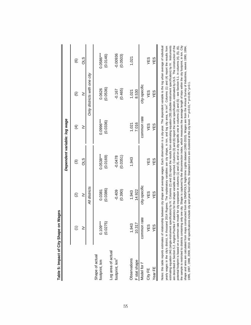
(1)
(2)
(3)
(4)
(5)
(6)
IVIV
OL
SIV
IVO
LS
Sh
ap
e o
f a
ctu
al
foo
tpri
nt,
km
0.1
09
***
0.0
38
10
.05
38
***
0.0
99
6**
*0
.06
26
0.0
58
6**
*
(0.0
27
5)
(0.0
38
6)
(0.0
16
9)
(0.0
33
6)
(0.0
53
6)
(0.0
14
6)
Lo
g a
rea
of
actu
al
foo
tpri
nt,
km
2-0
.40
9-0
.04
78
-0.1
67
-0.0
09
36
(0.3
90
)(0
.03
51
)(0
.46
5)
(0.0
50
3)
Ob
se
rva
tio
ns
1,9
43
1,9
43
1,9
43
1,0
21
1,0
21
1,0
21
F s
tat
sh
ap
e1
0.3
17
14
.92
27
.01
68
.53
0
Mo
de
l fo
r r
co
mm
on
ra
tecity-s
pe
cific
co
mm
on
ra
tecity-s
pe
cific
City F
EY
ES
YE
SY
ES
YE
SY
ES
YE
S
Ye
ar
FE
YE
SY
ES
YE
SY
ES
YE
SY
ES
Ta
ble
5:
Imp
ac
t o
f C
ity S
ha
pe
on
Wa
ge
s
All
dis
tric
tsO
nly
dis
tric
ts w
ith
on
e c
ity
Note
s:
this
table
report
sestim
ate
sof
rela
tionship
betw
een
city
shape
and
avera
ge
wages.
Each
observ
ation
isa
city-
year.
The
dependent
variable
isth
elo
gurb
an
avera
ge
of
indiv
idual
yearly
wages
inth
ecity'
sdis
tric
t,in
thousand
2014
Rupees.
The
expla
nato
ryvariable
sare
city
shape,
inkm
,and
log
city
are
a,
inkm
2.
Colu
mns
(1)
and
(4)
report
the
results
from
estim
ating
equation
(44)
(sin
gle
-instr
um
ent
specific
ation)
by
IV.
Colu
mns
(2)
and
(5)
report
the
results
from
estim
ating
equation
(39)
(double
-instr
um
ent
specific
ation)
by
IV.
Instr
um
ents
are
described in S
ection 5
.2. A
ngrist-
Pis
chke F
sta
tistics for
the s
hape v
ariable
are
report
ed. C
olu
mns (
3)
and (
6)
report
the s
am
e s
pecific
ation, estim
ate
d b
y O
LS
. T
he c
onstr
uction o
f th
e
pote
ntialfo
otp
rint
isbased
on
acom
mon
rate
modelfo
rcity
expansio
nin
colu
mns
(1)
and
(4),
and
on
acity-
specific
one
incolu
mns
(2)
and
(5)
-see
Section
5.1
.In
colu
mns
(4),
(5),
(6),
the
sam
ple
isre
str
icte
dto
dis
tric
tsconta
inin
gonly
one
city.
Shape
iscaptu
red
by
the
dis
connection
index,
whic
hm
easure
sth
eavera
ge
length
of
trip
sw
ithin
the
city
footp
rint,
inkm
.C
ity
shape
and
are
aare
calc
ula
ted
from
maps
constr
ucte
dfr
om
the
DM
SP
/OLS
Nig
ht-
tim
eLig
hts
data
set
(1992-2
010).
Wages
are
from
the
Annual
Surv
ey
of
Industr
ies,
waves
1990,
1994,
1995, 1997, 1998, 2009, 2010. A
ll specific
ations inclu
de c
ity
and y
ear
fixed e
ffects
. S
tandard
err
ors
are
clu
ste
red a
t th
e c
ity
level. *
** p
<0.0
1,*
* p<
0.0
5,*
p<
0.1
.
De
pe
nd
en
t v
ari
ab
le:
log
wa
ge
55

(1)
(2)
(3)
(4)
(5)
(6)
IVIV
OL
SIV
IVO
LS
Sh
ap
e o
f a
ctu
al
foo
tpri
nt,
km
-0.0
10
7-0
.59
5-0
.00
01
18
-0.0
10
1-0
.51
6*
-0.0
09
96
(0.1
52
)(0
.39
1)
(0.0
49
3)
(0.2
08
)(0
.28
2)
(0.0
71
9)
Lo
g a
rea
of
actu
al
foo
tpri
nt,
km
2-1
.47
3-0
.01
01
-0.8
65
-0.0
52
7
(1.4
00
)(0
.08
21
)(0
.86
4)
(0.1
05
)
Ob
se
rva
tio
ns
83
98
40
84
14
45
44
54
45
F s
tat
sh
ap
e8
.46
61
1.1
30
5.1
35
16
.81
7
Sh
ap
e o
f a
ctu
al
foo
tpri
nt,
km
-0.0
17
4-0
.67
4-0
.00
78
6-0
.01
96
-0.5
91
*-0
.00
90
4
(0.1
71
)(0
.42
6)
(0.0
56
3)
(0.2
39
)(0
.32
1)
(0.0
80
7)
Lo
g a
rea
of
actu
al
foo
tpri
nt,
km
2-1
.58
00
.00
56
8-0
.97
4-0
.03
57
(1.5
29
)(0
.09
46
)(0
.98
2)
(0.1
20
)
Ob
se
rva
tio
ns
83
98
40
84
14
45
44
54
45
F s
tat
sh
ap
e8
.46
61
1.1
30
5.1
35
16
.81
7
Mo
de
l fo
r r
co
mm
on
ra
tecity-s
pe
cific
co
mm
on
ra
tecity-s
pe
cific
City F
EY
ES
YE
SY
ES
YE
SY
ES
YE
SY
ea
r F
EY
ES
YE
SY
ES
YE
SY
ES
YE
S
All
dis
tric
tsO
nly
dis
tric
ts w
ith
on
e c
ity
A.
De
pe
nd
en
t v
ari
ab
le:
log
ye
arl
y r
en
t p
er
sq
ua
re m
ete
r
B.
De
pe
nd
en
t v
ari
ab
le:
log
ye
arl
y r
en
t p
er
sq
ua
re m
ete
r, u
pp
er
50
%
Note
s:
this
table
report
sestim
ate
sof
rela
tionship
betw
een
city
shape
and
avera
ge
housin
gre
nts
.E
ach
observ
ation
isa
city-
year.
Inpanel
A,
the
dependent
variable
isth
elo
gurb
an
avera
ge
of
housin
gre
nt
per
square
mete
rin
the
city'
sdis
tric
t,in
2014
Rupees.
InpanelB
the
dependent
variable
isanalo
gous,
but
the
avera
ge
iscalc
ula
ted
consid
ering
only
the
top
50%
of
the
dis
tric
t'sdis
trib
ution
of
rents
per
square
mete
r.T
he
expla
nato
ryvariable
sare
city
shape,
inkm
,and
log
city
are
a,
inkm
².C
olu
mns
(1)
and
(4)
report
the
results
from
estim
ating
equation
(44)
(sin
gle
-instr
um
ent
specific
ation)
by
IV.C
olu
mns
(2)
and
(5)
report
the
results
from
estim
ating
equation
(39)
(double
-instr
um
entspecific
ation)
by
IV.
Instr
um
ents
are
described
inS
ection
5.2
.A
ngrist-
Pis
chke
Fsta
tistics
for
the
shape
variable
are
report
ed.
Colu
mns
(3)
and
(6)
report
the
sam
especific
ation,
estim
ate
dby
OLS
.T
he
constr
uction
of
the
pote
ntial
footp
rint
isbased
on
acom
mon
rate
modelfo
rcity
expansio
nin
colu
mns
(1)
and
(4),
and
on
acity-
specific
one
incolu
mns
(2)
and
(5)
-see
Section
5.1
.In
colu
mns
(4),
(5),
(6),
the
sam
ple
isre
str
icte
dto
dis
tric
tsconta
inin
gonly
one
city.
Shape
iscaptu
red
by
the
dis
connection
index,
whic
hm
easure
sth
eavera
ge
length
of
trip
sw
ithin
the
city
footp
rint,
inkm
.C
ity
shape
and
are
aare
calc
ula
ted
from
maps
constr
ucte
dfr
om
the
DM
SP
/OLS
Nig
ht-
tim
eLig
hts
data
set(1
992-2
010).
Housin
gre
nts
are
from
the
NS
SH
ousehold
Consum
er
Expenditure
Surv
ey,
rounds
62 (
2005-2
006),
63 (
2006-2
007)
and 6
4 (
2007-2
008).
All
specific
ations inclu
de c
ity
and y
ear
fixed e
ffects
. S
tandard
err
ors
are
clu
ste
red a
t th
e c
ity
level. *
** p
<0.0
1,*
* p<
0.0
5,*
p<
0.1
.
Ta
ble
6:
Imp
ac
t o
f C
ity S
ha
pe
on
Ho
us
ing
Re
nts
56

(1)
(2)
(3)
(4)
(5)
(6)
IVIV
IVIV
IVIV
No
rm.
sh
ap
e
-32
7.6
***
-30
6.2
***
-20
4.8
***
-27
5.6
***
-25
4.3
***
-13
6.3
***
(10
3.8
)(9
8.4
6)
(54
.16
)(9
3.2
9)
(89
.68
)(4
5.0
2)
No
rm.
sh
ap
e x
urb
an
ro
ad
de
nsity,
19
81
1.9
55
**1
.84
8**
1.4
85
***
(0.8
27
)(0
.77
9)
(0.4
51
)
No
rm.
sh
ap
e x
sta
te u
rba
n r
oa
d d
en
sity,
19
91
3.1
5e
-06
0.0
00
13
80
.00
06
38
**
(0.0
00
33
9)
(0.0
00
31
9)
(0.0
00
31
5)
Ob
se
rva
tio
ns
1,1
26
1,1
26
1,1
26
1,1
18
1,1
18
1,1
18
F s
tat
sh
ap
e8
.73
28
.46
11
7.3
33
22
.85
62
1.1
20
30
.24
6
F s
tat
inte
ractio
n t
erm
44
.64
24
5.4
21
48
.66
12
63
.61
02
54
.55
14
18
.75
3
No
rm.
sh
ap
e
-99
.33
***
-94
.23
***
-52
.63
***
-83
.63
***
-78
.21
***
-35
.37
***
(34
.36
)(3
3.2
3)
(12
.09
)(2
8.6
1)
(27
.96
)(9
.46
9)
No
rm.
sh
ap
e x
urb
an
ro
ad
de
nsity,
19
81
1.6
71
**1
.60
7**
1.2
31
***
(0.8
31
)(0
.79
7)
(0.4
30
)
No
rm.
sh
ap
e x
sta
te u
rba
n r
oa
d d
en
sity,
19
91
0.0
00
10
90
.00
02
14
0.0
00
75
7**
(0.0
00
38
8)
(0.0
00
36
8)
(0.0
00
31
5)
Ob
se
rva
tio
ns
1,1
26
1,1
26
1,1
26
1,1
18
1,1
18
1,1
18
F s
tat
sh
ap
e7
.70
57
.37
22
3.9
96
15
.48
31
4.3
75
43
.60
5
F s
tat
inte
ractio
n t
erm
49
.08
34
9.8
34
50
.45
92
78
.32
62
66
.60
34
85
.78
1
Mo
de
l fo
r r
co
mm
on
ra
teco
mm
on
ra
tecity-s
pe
cific
co
mm
on
ra
teco
mm
on
ra
tecity-s
pe
cific
City F
EY
ES
YE
SY
ES
YE
SY
ES
YE
S
Ye
ar
FE
YE
SY
ES
YE
SY
ES
YE
SY
ES
Ye
ar
FE
x B
an
ks in
19
81
NO
YE
SY
ES
NO
YE
SY
ES
Ta
ble
7:
Inte
rac
tio
ns
of
Cit
y S
ha
pe
wit
h I
nfr
as
tru
ctu
re
De
pe
nd
en
t v
ari
ab
le:
po
pu
lati
on
de
ns
ity
A.
Sh
ap
e M
etr
ic:
Dis
co
nn
ec
tio
n
B.
Sh
ap
e M
etr
ic:
Ra
ng
e
Note
s:
this
table
investigate
sth
eim
pact
of
shape,
inte
racte
dw
ith
infr
astr
uctu
re,
on
popula
tion
density.
Each
observ
ation
isa
city-
year.
All
colu
mns
report
IVestim
ate
sof
aspecific
ation
sim
ilar
toequation
(42)
(sin
gle
-instr
um
ent
specific
ation),
augm
ente
dw
ith
an
inte
raction
betw
een
norm
aliz
ed
shape
and
diffe
rent
infr
astr
uctu
repro
xie
s.
The
dependent
variable
ispopula
tion
density,
inth
ousands
of
inhabitants
per
km
2.
The
constr
uction
of
the
pote
ntial
footp
rint
isbased
on
acom
mon
rate
model
for
city
expansio
nin
colu
mns
(1),
(2),
(4),
(5)
and
on
acity-
specific
one
incolu
mns
(3)
and
(6)
-see
Section
5.1
.A
ngrist-
Pis
chke
Fsta
tistics
for
the
shape
variable
and
for
the
inte
raction
term
are
report
ed
ineach
colu
mn.
The
shape
metr
ics
consid
ere
dare
norm
aliz
ed
dis
connection
inP
anel
A,
and
norm
aliz
ed
range
inP
anelB
.D
isconnection
isth
eavera
ge
length
ofw
ithin
-city
trip
s.R
ange
isth
em
axim
um
length
ofw
ithin
-city
trip
s.In
colu
mns
(1)
,(2
)and
(3),
norm
aliz
ed
shape
isin
tera
cte
dw
ith
urb
an
road
density
inth
ecity,
as
report
ed
inth
e1981
Census.
Incolu
mns
(4),
(5),
and
(6),
norm
aliz
ed
shape
isin
tera
cte
dw
ith
sta
teurb
an
road
density
inye
ar
1991
(sourc
e:
Min
istr
yof
Road
Tra
nsport
and
Hig
hw
ays
).C
ity
shape
and
are
aare
calc
ula
ted
from
maps
constr
ucte
dfr
om
the
DM
SP
/OLS
Nig
ht-
tim
eLig
hts
data
set
(1992-2
010)
and
U.S
.A
rmy
maps
(1951).
Popula
tion
isdra
wn
from
the
Census
of
India
(1951,
1991,
2001,
2011).
All
specific
ations
inclu
de
city
and
year
fixed
effects
.S
pecific
ations
incolu
mns
(2),
(3),
(5)
and
(6)
als
oin
clu
de
year
fixed
effects
inte
racte
dw
ith
the
num
ber
of
banks
in
1981. S
tandard
err
ors
are
clu
ste
red a
t th
e c
ity
level. *
** p
<0.0
1,*
* p<
0.0
5,*
p<
0.1
.
57

(1)
(2)
(3)
(4)
(5)
(6)
IVIV
OL
SIV
IVO
LS
Sh
ap
e
of
actu
al
foo
tpri
nt,
km
-0.0
25
3-0
.13
4**
-0.0
35
3**
-0.0
50
2**
*-0
.11
3**
-0.0
49
8**
*
(0.0
17
1)
(0.0
54
0)
(0.0
15
8)
(0.0
18
5)
(0.0
56
1)
(0.0
15
9)
Lo
g a
rea
of
actu
al
foo
tpri
nt,
km
20
.59
20
.13
4*
0.2
64
0.0
50
1
(0.4
92
)(0
.07
81
)(0
.63
3)
(0.0
88
4)
Ob
se
rva
tio
ns
94
69
46
94
69
46
94
69
46
F s
tat
sh
ap
e1
01
6.1
98
50
.12
61
01
6.1
98
50
.12
6
Mo
de
l fo
r r
co
mm
on
ra
tecity-s
pe
cific
co
mm
on
ra
tecity-s
pe
cific
City F
EY
ES
YE
SY
ES
YE
SY
ES
YE
SY
ea
r F
EY
ES
YE
SY
ES
YE
SY
ES
YE
S
Ta
ble
8:
Imp
ac
t o
f C
ity S
ha
pe
on
Slu
m P
op
ula
tio
n
Lo
g s
lum
po
pu
lati
on
Lo
g s
lum
po
pu
lati
on
sh
are
Note
s:
this
table
report
sestim
ate
sof
rela
tionship
betw
een
city
shape
and
slu
mpopula
tion.
Each
observ
ation
isa
city-
year.
Colu
mns
(1)
and
(4)
report
the
results
from
estim
ating
equation
(44)
(sin
gle
-instr
um
ent
specific
ation)
by
IV.
Colu
mns
(2)
and
(5)
report
the
results
from
estim
ating
equation
(39)
(double
-instr
um
ent
specific
ation)
by
IV.
Colu
mns
(3)
and
(6)
report
the
sam
especific
ation,
estim
ate
dby
OLS
.T
he
expla
nato
ryvariable
sare
shape,
inkm
,and
log
city
are
a,
inkm
².In
str
um
ents
are
described
inS
ection
5.2
.A
ngrist-
Pis
chke
Fsta
tistics
for
the
shape
variable
are
report
ed.
The
constr
uction
of
the
pote
ntialfo
otp
rint
isbased
on
acom
mon
rate
modelfo
rcity
expansio
nin
colu
mns
(1)
and
(4)
and
on
acity-
specific
one
incolu
mns
(2)
and
(5)
-see
Section
5.1
.T
he
dependentvariable
sare
log
slu
mpopula
tion
inth
ecity
(colu
mns
(1),
(2),
(3))
,lo
gofth
eshare
of
slu
mto
tota
lpopula
tion
in
the
city
(colu
mns
(4),
(5),
(6))
.D
ata
on
slu
ms
isdra
wn
from
the
1991,
2001,
and
2011
Census.
Shape
iscaptu
red
by
the
dis
connection
index,
whic
hm
easure
sth
eavera
ge
length
of
trip
sw
ithin
the
city
footp
rint,
inkm
.C
ity
shape
and
are
aare
calc
ula
ted
from
maps
constr
ucte
dfr
om
the
DM
SP
/OLS
Nig
ht-
tim
eLig
hts
data
set
(1992-2
010).
All
specific
ations
inclu
de
city
and y
ear
fixed e
ffects
. S
tandard
err
ors
are
clu
ste
red a
t th
e c
ity
level. *
** p
<0.0
1,*
* p<
0.0
5,*
p<
0.1
.
58

Table 9: Impact of City Shape on the Number of Employment Subcenters, 2005
(1) (2) (3)
IV IV OLS
Subcenters /km2 Log subcenters Log subcenters
Norm. shape of actual footprint -0.317
(0.455)
Shape of actual footprint, km -0.0623* -0.0579***
(0.0377) (0.0154)
Log area of actual footprint, km2
0.606*** 0.571***
(0.124) (0.0567)
Observations 187 187 187
F stat shape 4.34 6.50
Model for r common rate city-specific
Notes: This table investigates the cross-sectional relationship between city shape, city area, and the number of employment
subcenters in year 2005. Each observation is a city in year 2005. The dependent variables are the number of subcenters per
km² (column (1)) and the log number of employment subcenters (columns (2) and (3)). Column (1) reports estimates from a
cross-sectional version of equation (42) (single-instrument specification), estimated by IV. Column (2) reports estimates from a
cross-sectional version of equation (39) (double-instrument specification), estimated by IV. Column (3) presents the same
specification, estimated by OLS. The construction of the potential footprint is based on a common rate model for city
expansion in column (1), and on a city-specific one in in column (2) - see Section 5.1. Angrist-Pischke F statistics for the shape
variable are reported. Shape is measured by the disconnection index, as the average length of trips within the city footprint, in
km. The procedure used to determine the number of subcenters in each city is drawn from McMillen (2001) and detailed in the
Appendix. Data on the spatial distribution of employment is derived from the urban Directories of Establishments, from the
2005 Economic Census. City shape and area are calculated from maps constructed from the DMSP/OLS Night-time Lights
dataset, in year 2005.
59

(1)
(2)
(3)
(4)
(5)
(6)
OL
SO
LS
OL
SO
LS
OL
SO
LS
No
rm.
sh
ap
e o
f
actu
al fo
otp
rin
t
Sh
ap
e o
f
actu
al
foo
tpri
nt
km
Lo
g a
rea
of
actu
al fo
otp
rin
t
km
²
No
rm.
sh
ap
e o
f
actu
al fo
otp
rin
t
Sh
ap
e o
f a
ctu
al
foo
tpri
nt
km
Lo
g a
rea
of
actu
al fo
otp
rin
t
km
²
No
rm.
sh
ap
e o
f p
ote
ntia
l fo
otp
rin
t0
.43
5**
*0
.33
7**
*
(0.1
23
)(0
.11
7)
No
rm.
sh
ap
e o
f p
ote
ntia
l fo
otp
rin
t-0
.09
08
**-0
.05
71
x F
AR
(0.0
45
2)
(0.0
37
1)
Lo
g p
roje
cte
d h
isto
ric p
op
ula
tio
n2
.99
81
.98
4**
1.3
22
1.0
86
*
(2.7
58
)(0
.79
5)
(1.8
41
)(0
.64
7)
Lo
g p
roje
cte
d h
isto
ric p
op
ula
tio
n-1
.95
8*
-0.6
86
**-1
.31
5*
-0.3
42
x F
AR
(1.0
23
)(0
.31
9)
(0.7
79
)(0
.27
0)
Sh
ap
e o
f p
ote
ntia
l fo
otp
rin
t, k
m0
.15
6-0
.18
60
.23
50
.09
28
(1.1
82
)(0
.23
3)
-0.6
71
(0.1
87
)
Sh
ap
e o
f p
ote
ntia
l fo
otp
rin
t, k
m
0.6
65
0.1
35
0.6
17
**0
.02
44
x F
AR
(0.4
87
)(0
.10
6)
(0.2
79
)(0
.08
10
)
Ob
se
rva
tio
ns
1,1
83
1,1
83
1,1
83
1,1
83
1,1
83
1,1
83
Mo
de
l fo
r r
co
mm
on
ra
tecity-s
pe
cific
city-s
pe
cific
co
mm
on
ra
tecity-s
pe
cific
city-s
pe
cific
FA
Ra
ve
rag
ea
ve
rag
ea
ve
rag
ere
sid
en
tia
lre
sid
en
tia
lre
sid
en
tia
l
City F
EY
ES
YE
SY
ES
YE
SY
ES
YE
S
Ye
ar
FE
YE
SY
ES
YE
SY
ES
YE
SY
ES
Ta
ble
10
: U
rba
n F
orm
an
d F
loo
r A
rea
Ra
tio
s
A.
Fir
st-
sta
ge
im
pa
ct
of
FA
Rs
on
cit
y s
ha
pe
Note
s:
each
observ
ation
isa
city-
year.
PanelA
of
this
table
report
sestim
ate
sof
the
firs
t-sta
ge
rela
tionship
betw
een
Flo
or
Are
aR
atios,
city
shape,
and
are
a.
Colu
mns
(1),
(2),
(3)
and
(4),
(5),
(6),
panelA
,re
port
the
sam
especific
ations
report
ed
incolu
mns
(4),
(5),
(6),
panelC
,T
able
2,w
ith
the
additio
nofin
tera
ctions
betw
een
each
instr
um
entand
FA
Rs.F
AR
sare
dra
wn
from
Sridhar
(2010)
and
corr
espond
toth
em
axim
um
allo
wed
Flo
or
Are
aR
atios
ineach
city
as
of
the
mid
-2000s.
FA
Rs
are
expre
ssed
as
ratios
of
the
tota
lfloor
are
aof
abuild
ing
over
the
are
aof
the
plo
ton
whic
hit
sits.
Colu
mns
(1),
(2),
(3)
consid
er
the
avera
ge
of
resid
ential
and
non-r
esid
ential
FA
Rs,
while
colu
mns
(4),
(5),
(6)
only
consid
er
resid
ential
FA
Rs.
Shape
iscaptu
red
by
the
dis
connection
index,
whic
hm
easure
sth
eavera
ge
length
of
trip
sw
ithin
the
city
footp
rint,
inkm
.C
ity
shape
and
are
aare
calc
ula
ted
from
maps
constr
ucte
dfr
om
the
DM
SP
/OLS
Nig
ht-
tim
eLig
hts
data
set
(1992-2
010)
and
U.S
.A
rmy
maps
(1951).
Popula
tion
isfr
om
the
Census
(1951,
1991,
2001,
2011).
Popula
tion
density
ism
easure
din
thousands
of
inhabitants
per
km
2.
All
specific
ations
inclu
de
city
and
year
fixed e
ffects
. S
tandard
err
ors
are
clu
ste
red a
t th
e c
ity
level. *
** p
<0.0
1,*
* p<
0.0
5,*
p<
0.1
.
60

Ta
ble
10
(c
on
tin
ue
d):
Urb
an
Fo
rm a
nd
Flo
or
Are
a R
ati
os
IVIV
OL
SIV
IVO
LS
Po
pu
latio
n
De
nsity
Lo
g p
op
ula
tio
nL
og
po
pu
latio
nP
op
ula
tio
n
De
nsity
Lo
g p
op
ula
tio
nL
og
po
pu
latio
n
No
rm.
sh
ap
e o
f a
ctu
al fo
otp
rin
t-9
7.4
9-8
5.4
6
(10
2.5
)(1
08
.1)
No
rm.
sh
ap
e o
f a
ctu
al fo
otp
rin
t -1
0.9
1-1
6.8
9
x F
AR
(43
.88
)(4
5.1
2)
Sh
ap
e o
f a
ctu
al fo
otp
rin
t, k
m-0
.09
79
0.0
50
9-0
.27
1**
0.0
28
3
(0.1
24
)(0
.03
12
)(0
.12
2)
(0.0
28
5)
Sh
ap
e o
f a
ctu
al fo
otp
rin
t, k
m
0.0
02
90
-0.0
16
00
.06
88
*-0
.00
76
7
x F
AR
(0.0
47
2)
(0.0
12
9)
(0.0
37
1)
(0.0
10
3)
Lo
g a
rea
of
actu
al fo
otp
rin
t, k
m2
0.6
83
**0
.01
09
0.8
28
***
-0.0
44
3
(0.3
38
)(0
.12
8)
(0.3
08
)(0
.10
3)
Lo
g a
rea
of
actu
al fo
otp
rin
t, k
m2
0
.09
95
0.0
66
50
.00
16
60
.09
81
***
x F
AR
(0.1
16
)(0
.04
71
)(0
.08
86
)(0
.03
68
)
Ob
se
rva
tio
ns
25
22
52
25
22
52
25
22
52
Mo
de
l fo
r r
co
mm
on
ra
tecity-s
pe
cific
co
mm
on
ra
tecity-s
pe
cific
FA
Ra
ve
rag
ea
ve
rag
ea
ve
rag
ere
sid
en
tia
lre
sid
en
tia
lre
sid
en
tia
l
City F
EY
ES
YE
SY
ES
YE
SY
ES
YE
S
Ye
ar
FE
YE
SY
ES
YE
SY
ES
YE
SY
ES
B.
Imp
ac
t o
f c
ity
sh
ap
e a
nd
FA
Rs
on
po
pu
lati
on
Note
s:
each
observ
ation
isa
city-
year.
PanelB
report
sestim
ate
sof
the
rela
tionship
betw
een
Flo
or
Are
aR
atios,
shape,
and
popula
tion.
Colu
mns
(1),
(2),
(3)
and
(4),
(5),
(6),
panel
B,
report
the
sam
especific
ations
report
ed
incolu
mns
(4),
(5),
(6),
panelC
,T
able
3,
with
the
additio
nof
inte
ractions
betw
een
each
expla
nato
ryvariable
and
FA
Rs.
FA
Rs
are
dra
wn
from
Sridhar
(2010)
and
corr
espond
toth
em
axim
um
allo
wed
Flo
or
Are
aR
atios
ineach
city
as
of
the
mid
-2000s.
FA
Rs
are
expre
ssed
as
ratios
of
the
tota
lfloor
are
aof
abuild
ing
over
the
are
aofth
eplo
ton
whic
hit
sits.C
olu
mns
(1),
(2),
(3)
consid
er
the
avera
ge
ofre
sid
entialand
non-r
esid
entialF
AR
s,
while
colu
mns
(4),
(5),
(6)
only
consid
er
resid
entialF
AR
s.
Shape
iscaptu
red
by
the
dis
connection
index,
whic
hm
easure
sth
eavera
ge
length
of
trip
sw
ithin
the
city
footp
rint,
inkm
.C
ity
shape
and
are
aare
calc
ula
ted
from
maps
constr
ucte
d
from
the
DM
SP
/OLS
Nig
ht-
tim
eLig
hts
data
set(1
992-2
010)
and
U.S
.A
rmy
maps
(1951).
Popula
tion
isfr
om
the
Census
(1951,1991,
2001,2011).
Popula
tion
density
ism
easure
din
thousands o
f in
habitants
per
km
2. A
ll specific
ations inclu
de c
ity
and y
ear
fixed e
ffects
. S
tandard
err
ors
are
clu
ste
red a
t th
e c
ity
level. *
** p
<0.0
1,*
* p<
0.0
5,*
p<
0.1
.
61

(1) (2)
IV IV
Population density Log population
Norm. shape of actual footprint -348.4***
(118.0)
Shape of actual footprint, km -0.194***
(0.0596)
Log area of actual footprint, km2
0.973***
(0.222)
Observations 1,329 1,329
Number of id 432 432
F stat shape 9.115 26.699
Model for r common rate city-specific
City FE YES YES
Year FE YES YES
Initial shape x year FE YES YES
Appendix Table 1: Impact of Shape on Population, Robustness to Initial Shape x Year Fixed Effects
Notes: this table presents a robustness check to Table 3, augmenting the specification with year fixed effects interacted with initial shape. Each
observation is a city-year. Columns (1) and (2) are equivalent to columns (4) and (5), panel C, in Table 3. Column (1) reports IV estimates of the
relationship between normalized city shape and population density, in thousand inhabitants per km2. Column (2) reports IV estimates of the
relationship between city shape and area, and log population. Shape is captured by the disconnection index, which measures the average length of
trips within the city footprint, in km. The construction of the potential footprint is based on a common rate model for city expansion in column (1) and
on a city-specific one in column (2) – see Section 5.1. City shape and area are calculated from maps constructed from the DMSP/OLS Night-time
Lights dataset (1992-2010) and U.S. Army maps (1951). Population is drawn from the Census of India (1951, 1991, 2001, 2011). All specifications
include city and year fixed effects, as well as year fixed effects interacted with the city’s disconnection index measured in the initial year of the panel
(1951). Standard errors are clustered at the city level. *** p<0.01,** p<0.05,* p<0.1.
62

(1)
(2)
(3)
(4)
IVIV
IVIV
Sh
ap
e o
f a
ctu
al fo
otp
rin
t, k
m0
.09
89
***
0.0
11
60
.10
8**
0.0
39
3
(0.0
27
2)
(0.0
42
0)
(0.0
42
1)
(0.0
76
8)
Lo
g a
rea
of
actu
al fo
otp
rin
t, k
m2
-0.3
58
-0.1
64
(0.3
95
)(0
.46
5)
F s
tat
sh
ap
e6
.68
91
1.4
80
4.1
58
5.5
18
Ob
se
rva
tio
ns
1,9
43
1,9
43
1,0
21
1,0
21
Sh
ap
e o
f a
ctu
al fo
otp
rin
t, k
m-0
.03
05
-0.7
4-0
.03
19
-0.6
69
*
(0.2
42
)(0
.48
2)
(0.3
63
)(0
.35
6)
Lo
g a
rea
of
actu
al fo
otp
rin
t, k
m2
-1.2
45
-0.5
62
(1.3
48
)(0
.80
2)
Ob
se
rva
tio
ns
84
18
41
44
54
45
F s
tat
sh
ap
e5
.65
06
.45
72
.97
47
.31
4
Mo
de
l fo
r r
co
mm
on
ra
tecity-s
pe
cific
co
mm
on
ra
tecity-s
pe
cific
City F
EY
ES
YE
SY
ES
YE
S
Ye
ar
FE
YE
SY
ES
YE
SY
ES
Initia
l sh
ap
e x
ye
ar
FE
YE
SY
ES
YE
SY
ES
All
dis
tric
tsO
nly
dis
tric
ts w
ith
on
e c
ity
B.
De
pe
nd
en
t v
ari
ab
le:
log
ye
arl
y r
en
t p
er
sq
ua
re m
ete
r
A.
De
pe
nd
en
t v
ari
ab
le:
log
wa
ge
Note
s:
this
table
pre
sents
aro
bustn
ess
check
toT
able
s5
and
6,
augm
enting
the
specific
ations
with
year
fixed
effects
inte
racte
dw
ith
initia
lshape.
Each
observ
ation
isa
city-
year.
InpanelA
the
dependent
variable
isth
elo
gurb
an
avera
ge
of
indiv
idualye
arly
wages
inth
ecity'
sdis
tric
t,in
thousand
2014
Rupees.
In
panel
Bth
edependent
variable
isth
elo
gurb
an
avera
ge
of
housin
gre
nts
per
m²
inth
ecity'
sdis
tric
t,in
2014
Rupees.
Colu
mns
(1),
(3)
report
the
results
from
estim
ating
equation
(44)
(sin
gle
-instr
um
ent
specific
ation)
by
IV.
Colu
mns
(2),
(4)
report
the
results
from
estim
ating
equation
(39)
(double
-instr
um
ent
specific
ation)
by
IV.
Instr
um
ents
are
described
inS
ection
5.2
.A
ngrist-
Pis
chke
Fsta
tistics
for
the
shape
variable
are
report
ed.
The
constr
uction
of
the
pote
ntial
footp
rint
is
based
on
acom
mon
rate
modelfo
rcity
expansio
nin
colu
mns
(1),
(3),
and
on
acity-
specific
one
incolu
mns
(2),
(4)
-see
Section
5.1
.In
colu
mns
(3)
and
(4),
the
sam
ple
isre
str
icte
dto
dis
tric
tsconta
inin
gonly
one
city.
Shape
iscaptu
red
by
the
dis
connection
index,
whic
hm
easure
sth
eavera
ge
length
of
trip
sw
ithin
the
city
footp
rint,
inkm
.C
ity
shape
and
are
aare
calc
ula
ted
from
maps
constr
ucte
dfr
om
the
DM
SP
/OLS
Nig
ht-
tim
eLig
hts
data
set
(1992-2
010).
Wages
are
from
the
Annual
Surv
ey
of
Industr
ies,
waves
1990,
1994,
1995,
1997,
1998,
2009,
2010.
Housin
gre
nts
are
from
the
NS
SH
ousehold
Consum
er
Expenditure
Surv
ey,
rounds
62
(2005-2
006),
63
(2006-2
007)
and
64
(2007-2
008).
All
specific
ations
inclu
de
city
and
year
fixed
effects
,as
well
as
year
fixed
effects
inte
racte
dw
ith
the
city'
s d
isconnection index m
easure
d in the initia
l ye
ar
of th
e p
anel (1
951).
Sta
ndard
err
ors
are
clu
ste
red a
t th
e c
ity
level. *
** p
<0.0
1,*
* p<
0.0
5,*
p<
0.1
.
Ap
pe
nd
ix T
ab
le 2
: Im
pa
ct
of
Sh
ap
e o
n W
ag
es
an
d R
en
ts,
Ro
bu
stn
es
s t
o I
nit
ial
Sh
ap
e x
Ye
ar
Fix
ed
Eff
ec
ts
63

Appendix Table 3: Urban Form and Floor Area Ratios
(1) (2) (3) (4) (5) (6)
IV IV OLS IV IV OLS
Shape of actual
footprint, km 0.000290 0.0508 0.021 0.00515 0.0715* 0.0439**
(0.00741) (0.0409) (0.0140) (0.00914) (0.0401) (0.0199)
Log area of actual
footprint, km2
-0.190 -0.105* -0.280 -0.177**
(0.179) (0.0540) (0.176) (0.0876)
Observations 55 55 55 55 55 55
Model for r common rate city-specific common rate city-specific
FARs Determinants, 2005
Avg. FAR Residential FAR
Notes: This table investigates the cross-sectional relationship between city shape, city area, and Floor Area Ratios as of year 2005. Each observation is a city
in year 2005. Columns (1) and (4) estimate a cross-sectional version of equation (44) (single-instrument specification), with log FARs as a dependent
variable, estimated by IV. Columns (2) and (5) estimate a cross-sectional version of equation (39) (double-instrument specification), with log FARs as a
dependent variable, estimated by IV. Columns (3) and (6) present the same specification, estimated by OLS. FARs are drawn from Sridhar (2010) and
correspond to the maximum allowed Floor Area Ratios in each city as of the mid-2000s. FARs are expressed as ratios of the total floor area of a building
over the area of the plot on which it sits. Columns (1), (2), (3) consider the average of residential and non-residential FARs, while columns (4), (5), (6) only
consider residential FARs. Shape is captured by the disconnection index, which measures the average length of trips within the city footprint, in km. City
shape and area are calculated from maps constructed from the DMSP/OLS Night-time Lights dataset, in year 2005. Standard errors are clustered at the city
level. *** p<0.01,** p<0.05,* p<0.1.
64

(1)
(2)
(3)
(4)
(5)
IVIV
IVIV
IV
So
cia
l S
erv
ice
sS
erv
ice
sT
ran
sp
ort
an
d S
tora
ge
Re
tail
Ma
nu
factu
rin
g
Sh
ap
e o
f a
ctu
al fo
otp
rin
t, k
m0
.02
19
0.0
68
10
.11
10
.05
70
-0.0
95
7
(0.0
50
4)
(0.1
03
)(0
.10
0)
(0.0
45
7)
(0.0
67
4)
Ob
se
rva
tio
ns
68
46
84
68
46
84
68
4
F s
tat
sh
ap
e2
3.6
92
3.6
92
3.6
92
3.6
92
3.6
9
Me
an
of
sh
are
0.2
90
.06
0.0
50
.34
0.2
4
Mo
de
l fo
r r
co
mm
on
ra
teco
mm
on
ra
teco
mm
on
ra
teco
mm
on
ra
teco
mm
on
ra
te
City F
EY
ES
YE
SY
ES
YE
SY
ES
Ye
ar
FE
YE
SY
ES
YE
SY
ES
YE
S
Ap
pe
nd
ix T
ab
le 4
: Im
pa
ct
of
Cit
y S
ha
pe
on
Se
cto
ral
Sh
are
s
Note
s:
This
table
investigate
sth
ere
lationship
betw
een
city
shape
and
the
share
of
firm
sin
diffe
rent
secto
rs,
weig
hte
dby
num
ber
of
work
ers
.E
ach
observ
ation
isa
city-
year.
The
dependent
variable
isth
elo
gshare
of
work
ers
indiffe
rent
secto
rs,
derived
from
the
3rd
,4th
and
5th
Econom
icC
ensus.
Secto
rsare
defined
based
on
National
Industr
yC
lassific
ation
1-d
igit
codes:
socia
lserv
ices
(1),
serv
ices
(2),
transport
and
sto
rage
(3),
reta
il(4
),m
anufa
ctu
ring
(5).
Secto
rsw
ith
neglig
ible
(<0.0
07)
share
s(e
lectr
icity
and
gas,
constr
uction,
min
ing)
are
not
report
ed.
"Serv
ices"
secto
rin
clu
des:
financia
l,in
sura
nce,
real
esta
teand
busin
ess
serv
ices.
"Socia
lS
erv
ices"
secto
rin
clu
des:
com
munity,
socia
land
pers
onal
serv
ices.
See
Section
3.5
for
a
description
of
the
data
.C
ols
.(1
)to
(5)
report
the
results
from
estim
ating
equation
(44)
(sin
gle
-instr
um
ent
specific
ation)
by
IV.
Instr
um
ents
are
described
inS
ection
5.1
.F
sta
tistics
for
the
shape
variable
are
report
ed.
The
constr
uction
of
the
pote
ntialfo
otp
rint
isbased
on
acom
mon
rate
modelfo
rcity
expansio
n.
Shape
iscaptu
red
by
the
dis
connection
index,
whic
hm
easure
s
the
avera
ge
length
of
trip
sw
ithin
the
city
footp
rint,
inkm
.C
ity
shape
and
are
aare
calc
ula
ted
from
maps
constr
ucte
dfr
om
the
DM
SP
/OLS
Nig
ht-
tim
eLig
hts
data
set
(1992-2
010).
All
specific
ations inclu
de c
ity
and y
ear
fixed e
ffects
. S
tandard
err
ors
are
clu
ste
red a
t th
e c
ity
level. *
** p
<0.0
1,*
* p<
0.0
5,*
p<
0.1
.
65

66

67

Kolkata
Bengaluru
Shape metric Normalized
Normalized
remoteness, km
14.8 0.99
10.3 0.69
spin, km2
288.4 1.29
120.9 0.54
disconnection, km
20.2 1.35
14 0.94
range, km
62.5 4.18
36.6 2.45
68

constraineddevelopable
69

70

71