CISC667, F05, Lec22, Liao1 CISC 667 Intro to Bioinformatics (Fall 2005) Support Vector Machines I

CISC667, F05, Lec22, Liao 1

CISC 667 Intro to Bioinformatics(Fall 2005)

Support Vector Machines I


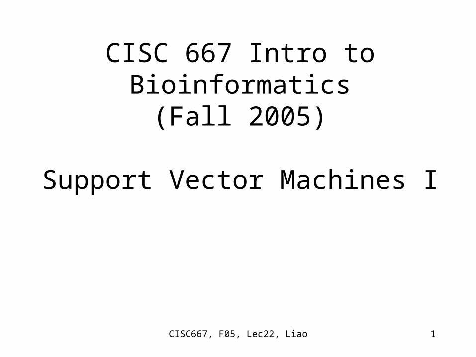
Terminologies• An object x is represented by a set of m attributes xi, 1 i

m.• A set of n training examples S = { (x1, y1), …, (xn, yn)},

where yi is the classification (or label) of instance xi. – For binary classification, yi ={1, +1}, and for k-class

classification, yi ={1, 2, …,k}. – Without loss of generality, we focus on binary classification.

• The task is to learn the mapping: xi yi

• A machine is a learned function/mapping/hypothesis h: xi h(xi , )

where stands for parameters to be fixed during training.

• Performance is measured as

E = (1/2n) i=1 to n |yi- h(xi , )|


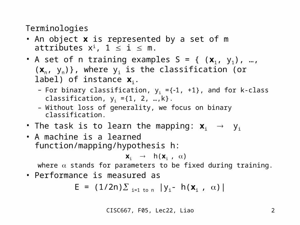
Linear SVMs: find a hyperplane (specified by normal vector w and perpendicular distance b to the origin) that separates the positive and negative examples with the largest margin.

Separating hyperplane (w, b)

Margin

Origin

w

b

w · xi + b > 0 if yi = +1

w · xi + b < 0 if yi = 1+

An unknown x is classified as sign(w · x + b)


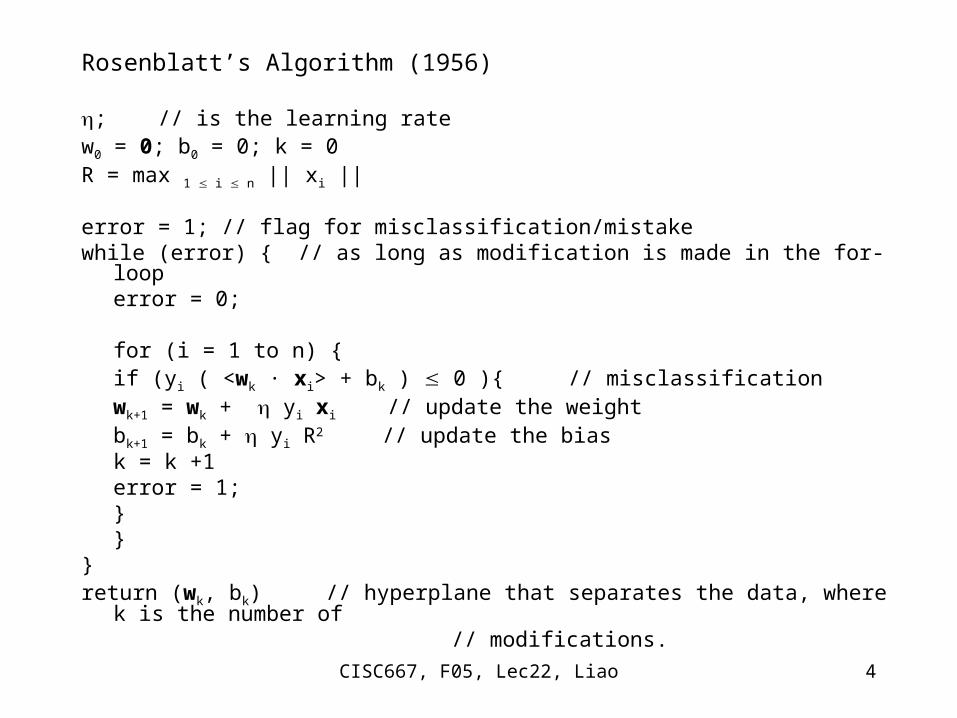
Rosenblatt’s Algorithm (1956)

; // is the learning ratew0 = 0; b0 = 0; k = 0R = max 1 i n || xi ||

error = 1; // flag for misclassification/mistakewhile (error) { // as long as modification is made in the for-loop

error = 0;

for (i = 1 to n) {if (yi ( <wk · xi> + bk ) 0 ){ // misclassification

wk+1 = wk + yi xi // update the weight bk+1 = bk + yi R2 // update the biask = k +1error = 1;

}}

}return (wk, bk) // hyperplane that separates the data, where k is the number of // modifications.


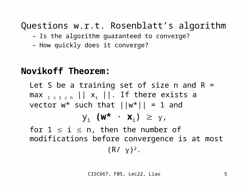
Questions w.r.t. Rosenblatt’s algorithm– Is the algorithm guaranteed to converge?

– How quickly does it converge?

Novikoff Theorem:

Let S be a training set of size n and R = max 1 i n || xi ||. If there exists a vector w* such that ||w*|| = 1 and

yi (w* · xi) ,

for 1 i n, then the number of modifications before convergence is at most

(R/ )2.


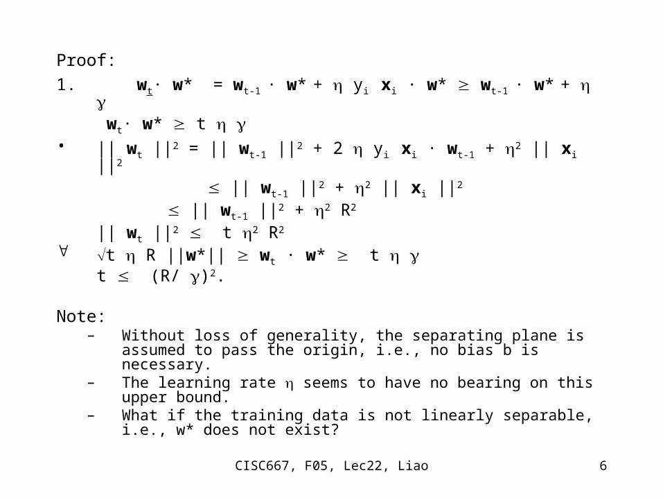
Proof:

1. wt· w* = wt-1 · w* + yi xi · w* wt-1 · w* + wt· w* t

• || wt ||2 = || wt-1 ||2 + 2 yi xi · wt-1 + 2 || xi ||2 || wt-1 ||2 + 2 || xi ||2

|| wt-1 ||2 + 2 R2 || wt ||2 t 2 R2

t R ||w*|| wt · w* t t (R/ )2.

Note: – Without loss of generality, the separating plane is assumed to pass the

origin, i.e., no bias b is necessary. – The learning rate seems to have no bearing on this upper bound. – What if the training data is not linearly separable, i.e., w* does not

exist?


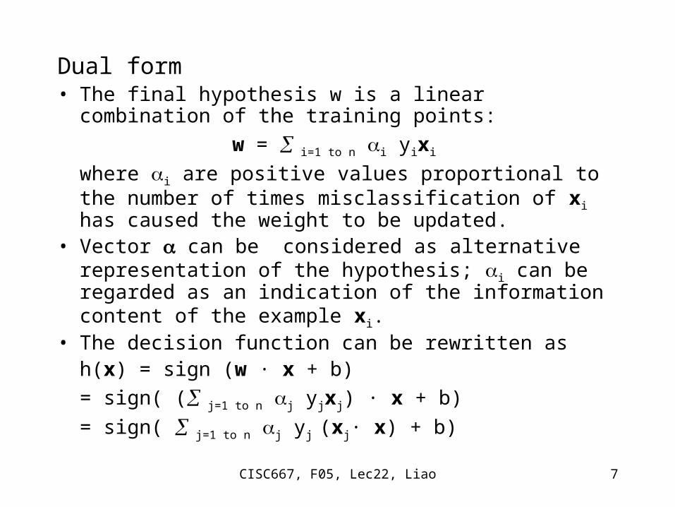
Dual form• The final hypothesis w is a linear combination of the

training points:

w = i=1 to n i yixi

where i are positive values proportional to the number of times misclassification of xi has caused the weight to be updated.

• Vector can be considered as alternative representation of the hypothesis; i can be regarded as an indication of the information content of the example xi.

• The decision function can be rewritten ash(x) = sign (w · x + b)

= sign( ( j=1 to n j yjxj) · x + b)

= sign( j=1 to n j yj (xj· x) + b)


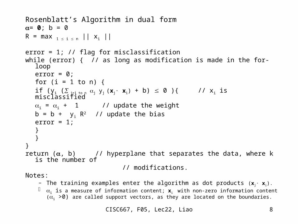
Rosenblatt’s Algorithm in dual form= 0; b = 0R = max 1 i n || xi ||

error = 1; // flag for misclassificationwhile (error) { // as long as modification is made in the for-loop

error = 0;for (i = 1 to n) {

if (yi ( j=1 to n j yj (xj· xi) + b) 0 ){ // xi is misclassifiedi = i + 1 // update the weight b = b + yi R2 // update the biaserror = 1;

}}

}return (, b) // hyperplane that separates the data, where k is the number of // modifications.Notes:

– The training examples enter the algorithm as dot products (xj· xi). i is a measure of information content; xi with non-zero information content (i >0) are called

support vectors, as they are located on the boundaries.


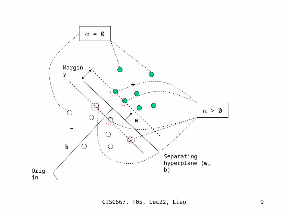
Separating hyperplane (w, b)

Margin

Origin

w

b

+

> 0

= 0


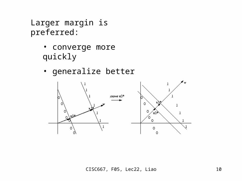
Larger margin is preferred:

• converge more quickly

• generalize better


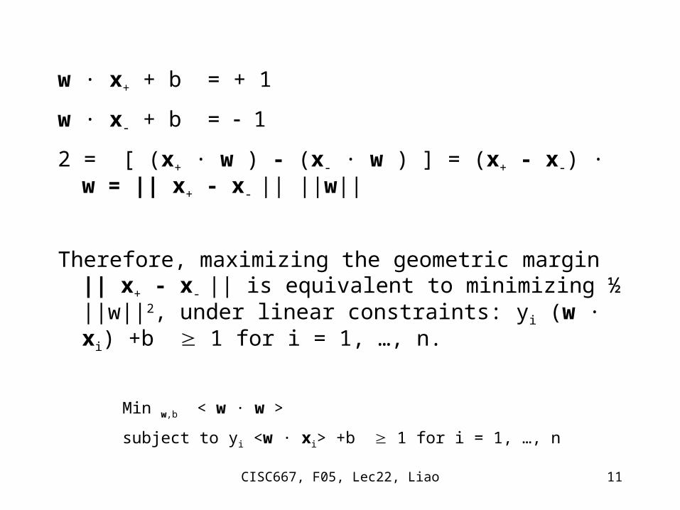
w · x+ + b = + 1

w · x- + b = 1

2 = [ (x+ · w ) - (x- · w ) ] = (x+ - x-) · w = || x+ - x- || ||w||

Therefore, maximizing the geometric margin || x+ - x- || is equivalent to minimizing ½ ||w||2, under linear constraints: yi (w · xi) +b 1 for i = 1, …, n.

Min w,b < w · w >

subject to yi <w · xi> +b 1 for i = 1, …, n


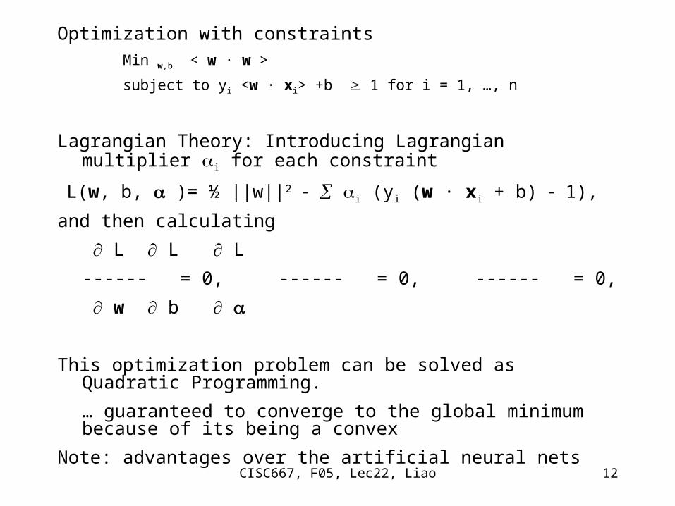
Optimization with constraints

Min w,b < w · w >

subject to yi <w · xi> +b 1 for i = 1, …, n

Lagrangian Theory: Introducing Lagrangian multiplier i for each constraint

L(w, b, )= ½ ||w||2 i (yi (w · xi + b) 1),

and then calculating

L L L

------ = 0, ------ = 0, ------ = 0,

w b

This optimization problem can be solved as Quadratic Programming.

… guaranteed to converge to the global minimum because of its being a convex

Note: advantages over the artificial neural nets


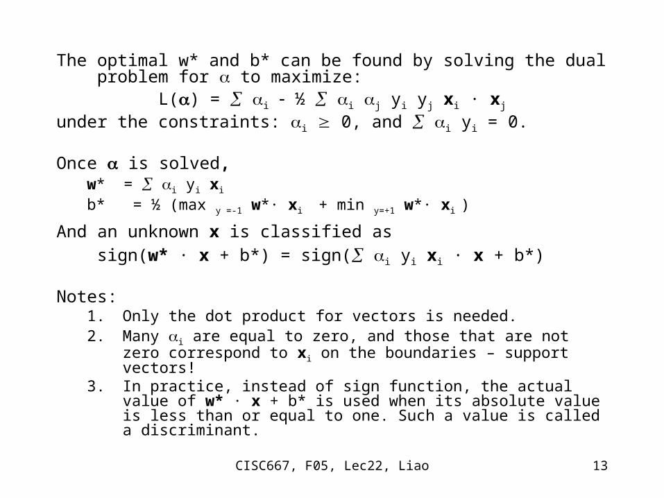
The optimal w* and b* can be found by solving the dual problem for to maximize:

L() = i ½ i j yi yj xi · xj

under the constraints: i 0, and i yi = 0.

Once is solved, w* = i yi xi b* = ½ (max y =-1 w*· xi + min y=+1 w*· xi )

And an unknown x is classified as sign(w* · x + b*) = sign( i yi xi · x + b*)

Notes:1. Only the dot product for vectors is needed.2. Many i are equal to zero, and those that are not zero correspond to xi

on the boundaries – support vectors! 3. In practice, instead of sign function, the actual value of w* · x + b* is

used when its absolute value is less than or equal to one. Such a value is called a discriminant.


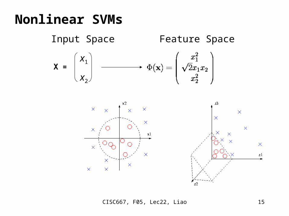
Non-linear mapping to a feature space

Φ( )

xi Φ(xi)Φ(xj)xj

L() = i ½ i j yi yj Φ (xi )·Φ (xj )


X =

Nonlinear SVMs

Input Space Feature Space

x1

x2


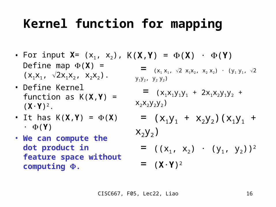
Kernel function for mapping

• For input X= (x1, x2), Define map (X) = (x1x1, 2x1x2, x2x2).

• Define Kernel function as K(X,Y) = (X·Y)2.

• It has K(X,Y) = (X) · (Y)

• We can compute the dot product in feature space without computing .

K(X,Y) = (X) · (Y)

= (x1 x1, 2 x1x2, x2 x2) · (y1 y1, 2 y1y2, y2 y2)

= (x1x1y1y1 + 2x1x2y1y2 + x2x2y2y2)

= (x1y1 + x2y2)(x1y1 + x2y2)

= ((x1, x2) · (y1, y2))2

= (X·Y)2


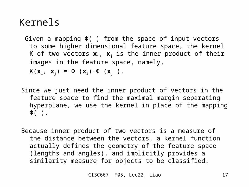
Kernels

Given a mapping Φ( ) from the space of input vectors to some higher dimensional feature space, the kernel K of two vectors xi, xj is the inner product of their images in the feature space, namely,

K(xi, xj) = Φ (xi)·Φ (xj ).

Since we just need the inner product of vectors in the feature space to find the maximal margin separating hyperplane, we use the kernel in place of the mapping Φ( ).

Because inner product of two vectors is a measure of the distance between the vectors, a kernel function actually defines the geometry of the feature space (lengths and angles), and implicitly provides a similarity measure for objects to be classified.


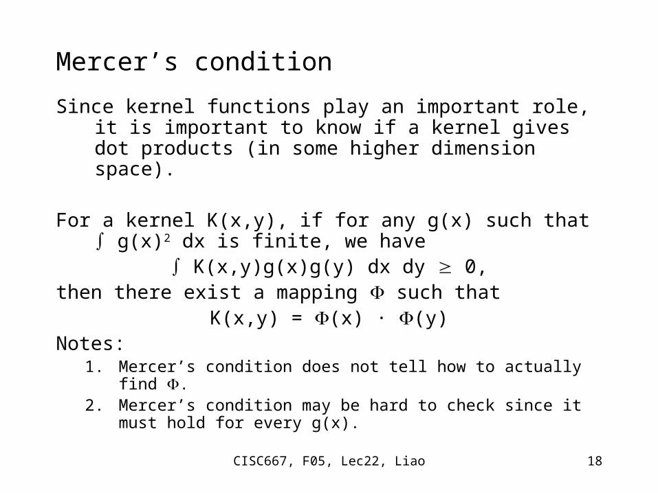
Mercer’s condition

Since kernel functions play an important role, it is important to know if a kernel gives dot products (in some higher dimension space).

For a kernel K(x,y), if for any g(x) such that g(x)2 dx is finite, we have

K(x,y)g(x)g(y) dx dy 0,then there exist a mapping such that

K(x,y) = (x) · (y)Notes:

1. Mercer’s condition does not tell how to actually find .2. Mercer’s condition may be hard to check since it must hold for

every g(x).


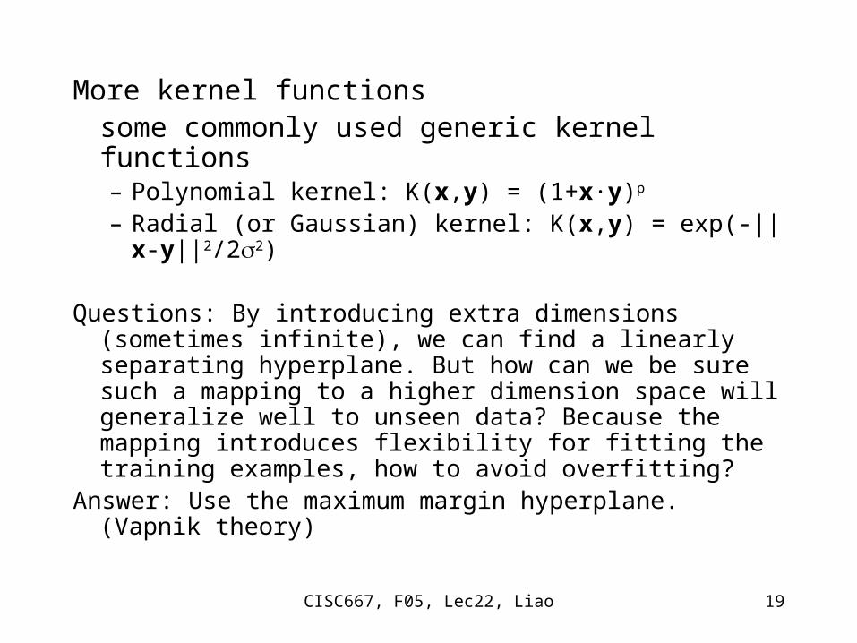
More kernel functionssome commonly used generic kernel functions– Polynomial kernel: K(x,y) = (1+x·y)p – Radial (or Gaussian) kernel: K(x,y) = exp(-||x-y||2/22)

Questions: By introducing extra dimensions (sometimes infinite), we can find a linearly separating hyperplane. But how can we be sure such a mapping to a higher dimension space will generalize well to unseen data? Because the mapping introduces flexibility for fitting the training examples, how to avoid overfitting?

Answer: Use the maximum margin hyperplane. (Vapnik theory)


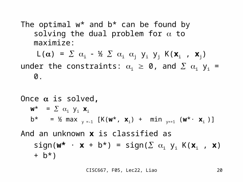
The optimal w* and b* can be found by solving the dual problem for to maximize:

L() = i ½ i j yi yj K(xi , xj)

under the constraints: i 0, and i yi = 0.

Once is solved, w* = i yi xi

b* = ½ max y =-1 [K(w*, xi) + min y=+1 (w*· xi )]

And an unknown x is classified as sign(w* · x + b*) = sign( i yi K(xi , x) + b*)


References and resources• Cristianini & Shawe-Tayor, “An introduction to

Support Vector Machines”, Cambridge University Press, 2000.

• www.kernel-machines.org– SVMLight– Chris Burges, A tutorial

• J.-P Vert, A 3-day tutorial• W. Noble, “Support vector machine applications

in computational biology”, Kernel Methods in Computational Biology. B. Schoelkopf, K. Tsuda and J.-P. Vert, ed. MIT Press, 2004.

http://www.kernel-machines.org/

Documents

CISC667, F05, Lec22, Liao1 CISC 667 Intro to Bioinformatics (Fall 2005) Support Vector Machines I