UCW95088PREPRINT

REDUCEDSTORAGEMATRIXMETHODS

IN STIFF ODESYSTEMS

Peter N. Brown

Alan C. Hindmarsh CIRCULATION COPIsUBJEGT TO RECALL

I?U lWO WEEKS

This paper was prepared for submission to theJournal of Applied Mathematics & Computation.

—

DISCLAIMER

This document was prepsred as an account of work sponsored by an agency of theUnited Statea Government. Neither the United Statea Government nor the Universityof California nor any of their employ% makes any warranty, express or implied, orassumes any legal liability or responsibility for the accuracy, completeness, or rrsefrrl-ness of any information, apparatus, product+or process disclosed, or represents thatits use would not infringe privately owned rights. Reference herein to any specificcommercial product.%proces%or service by trade name, trademark manufacturer, orotherwise, does not necessarily constitute or imply its endoraemen~ recommendation,or favoring by tbe United States Government or the University of California. Theviews and opinions of authors expressed herein do not necessarily state or reflecttboae of the United States Government or the University of California, and shall notbe used for advertising or product endor~ment purposea.

.

*

●

●

W3uced Storage N@trix Methods in Stiff ODE Systems*

Peter N. BrownDepartment of Mathematics

University of HoustonHouston, TX 77004

Alan C. Hindmarsh@mIWtin9 & Mathematics Research Div., L-316

Lawrence Livermore National LaboratoryLivermore, CA 94550

August 1986

.

s

*This work was performed under the auspices of the U.S. Department of Energyby the Lawrence Livermore National Laboratory under Contract W-7405-Eng-48.The first author was also suppxted in part by National Science InundationGrant IMS-8506651.

—

b

F@uced Storage Matrix Mthods in Stiff ODE Systems

.

*

8

ZEwI’RAc’r

Stiff initial-value ODE methods (e.g. BDF) normally require the Jacobianmatrix as part of a Newton or Newton-like iteration within each implicit timestep. Until recently, stiff methods have normally required the Jacobian to beformed and stored explicitly, whether the linear algebraic n@dmd used isdirect or iterative. But any iterative linear system method which involvesthe system matrix only in operator form can be rmde part of an inexact Newtonmethod within such a stiff ODE method in a manner that requires no explicitJacobian matrix storage. The result is a matrix-free stiff method. Suchcombinations, using BDF methods, have been implemented with three KrylovSubspace methods -- Arnoldi iteration (and its incomplete form, the IncompleteOrthogonalization MMIod or I@’I), CMRES (the Generalize Minimum RESidualmethod), and (X (the Conjugate Gradient method, assuming a symmetric positivedefinite matrix). Various practical matters (scaling, starting, stopping,etc.) are dealt with in the stiff ODE context.

In the context of general nonlinear algebraic systems, we provide sanetheoretical foundation for the cotiined Newton-Krylov method by givingconvergence results that include errors due to the difference quotientapproximation to the linear operator.

Earlier tests showed matrix-free methods to be quite effective for certainclasses of problems. Hmever, unless the spectrum of the problem Jacobian israther tightly clustered, the methods are not likely to have competitiveconvergence properties. ‘Ib improve their robustness, preconditioning has beenadded. We have qrimented with preconditioned Krylov subspace methods forODE systems that arise from time-dependent PDE systems by the mMxx3 oflines. Preconditioned matrices can be formed from the interaction of the PDEvariables (giving a block-diagonal matrix), and also from the spatialtrarqmrt terms (using SOR or the like). Using both together amounts to anoperator splitting approach. The additional matrix storage requirement can bereduced greatly by grouping the diagonal blocks in a natural way. Thediagonal blocks rquired (if not sup@ied by the user) are generated bydifference quotient operations. Preconditioned Arnoldi, @llUZ5, and CG methodshave been implemented in an experimental solver called LSODPKthat uses BDFmethods . !lksts on PDE-based problems show the methcds to be quite effectivein improving both speed and storage econo~ over traditional stiff methods,and over matrix-free methods without preconditioning.

—

“2-

1. Introduction

]n a previous paper [4], ye considered the use of Krylov-subspace projection

methods in solving large stiff systems of ordinary differential equations (ODE’S).

Typically, methods for solving stiff ODE systems are implicit, and so require the

solution of a nonlinear algebraic system of equations at each integration step.

Newton’s method (or some modification of it) appears to be the best general

approach to such systems, and this leads to solving several linear systems at

each step. For large problems, most of the work required for the integration is

in the linear algebra operations associated with these linear systems. In addi-

ti on, when using direct methods to solve the linear systems, much of the core

memory required is used for the storage of the coefficient matrix and its decom-

position factors. Alternatively, the Krylov methods are iterative linear system

solvers which do not require the storage of the coefficient matrix in any form,

and hence require far less storage than direct methods. All that is required is

the ability to perform coefficient matrix-vector multiplies. In [4], we referred to

the combined stiff ODEmethod/Krylov method as a nza.triz-free method, and dis-

cussed both theoretical and computational aspects of the combined algorithm.

In this paper, we will continue investigating these combined algorithms, with

particular emphasis on the importance of preconditioning the liiear systems

solved by the Krylov methods.

To be more specific, we will consider here the numerical soIution of the

ODE Initial Value ProbIem

a=f(f.Y) s v(%)=% (“=CVCU,IA’9. (1.1)

We will assume that the ODE in (1.1) is stiff, meaning that one or more strongly

damped modes are present, and will use the popular BDF {Backward

Differentiation Formula) methods to solve it. These methods have the general

form

.

*

●

-3-

% = 5 aavn-j + h~o$n , in = J (in ,yn), (1.2)j=l

where q is the method order. Since the BDF

step one must solve the algebraic system

methods are implicit, at each time

&/n-hp,j(tn,yn) - ~=o , q= f aJw-j , /%>0. -j=l

for ~n. We will actuaUy deal with an equivalent form of (1.3), namely

rn(zn) = zn -hf(tns%+p.%) = Q

in which ~ is defined by

% = h;n = (Yn-G)/ ~. .

The Newton iteration then has the form:

Let Zn(0) be an initial guess for ~.

For m =0,1,2, “ . “ until convergence:

An(m) ‘- ~(zn(m))

~(rn+l) = Zn(na) +Sn(m),

where the coefficient matrix P is some value of (or an approximation to a value

of)

F:(z) = l–hpo J(f,y) (y=q+@oz), (1.6)

with J(f ,y ) = d~ / @ , the system Jacobian matrix.

In [4j, we considered two K@ov-subspace projection methods for

approximately solving (1.5). These were AmLohfi’s A?goti~hm and the Incomplete

Othogondiza.ticm Methocf (IOM), both due primarily to Saad [17,18]. The prelim-

inary tests in [4] indicated the potential usefulness of these linear solvers on

ODE problems for which there is some clustering of the spectrum of the matrix

(1.3)

(1.4)

(1.5)

—

-4-

P, but also indicated the need for some form of preconditioning of the linear sys-

tems (1.5) in order for the combined BDF/Krylov method solver to be effective

on a much wider class of problems. Preconditioning tectilques must be chosen

with the particular problem features in mind, and also with a view to keeping the

storage requirements low. For problems arising from time-dependent partial

differential equation (PDE) systems, choices based on successive overrelaxation

(SOR), and on the interaction of the PDE variable at each spatial point are avail-

able.

Work that is closely related to ours includes that of Gear and Saad [9],

Who orighmlly proposed using Arnoldl’s Algorithm and IOM in sUM ODE solvers,

and Miranker and Chern [15] who considered the use of the Conjugate Gradient

Method in the solution of the model problem dy/ di = @ by BDF methods for

which J is symmetric and posithw definite. Additionally, Chan and Jackson [5]

have considered the use of Preconditioned Krylov-subspace projection methods

in ODE solvers. However, their methods differ from those considered here in

several respects. Frst, the basic Krylov methods considered in [5] are the COrV

jugafe l?esidu.cd Method (CR) and Orthornin ~) (cf. [8]). We note that CR applied

to (1.5) is only guaranteed to cmuerge when P is symmetric and positive definite,

while Orthornin (k) only requires that P is positive defilte for convergence. Chan

and Jackson argue that for symmetric problems (i.e. J = dj / @ symmetric) me

step size selectlon strategy of the ODE solver wiU normally choose h so that

l-h&&>O (1.7)

for all ~ (i=l, . . ., A’) an eigenvalve of J. Hence, in this case P=l -h~. J would

be positive definite. When J is nonsyrnrnetric, (1.7) holding for all Ai does not

imply P is positive defilte, as Chan and Jackson note. Thus, the application of

CR ~d Orthoti {k) to such linear systems may fail. Second these methods are

actually applied to the precondltiloned llnear systems, and so one must be

-5-

careful when choosing the preconditioning to be used so that the resulting sys-

tem has a matrix which is again positive definite, as Chan and Jackson also note.

In our setting, Arnoldi’s Algorithm and GMRES are guaranteed to converge when

the matrix P is nonsingular (whether or not it is positive defirite). ‘1’tis results in

a wider class of available preconditioning when using Arnoldi and GMRES.

The rest of the paper is organized as follows: Section 2 summarizes the

Newton and Newton-like iteration for the nonlinear system and the basic linear

iterations to be considered (Arnoldio GMRES, and CG), and includes a new result

on an incomplete version of GMRES. Section 3 gives some local convergence

results for the combined Newton/Krylov methods. Section 4 discusses scaled

preconditioned methods in general, and Section 5 describes specific precondi-

tioners suitable for ODE systems arising from certain PDE systems. Section 6

gives some numerical test results, using a modified version of the general pur-

pose ODE solver LSODE [13,14].

.

-6-

2 Preliminaries

In this section we introduce a class of Newton-1ike iteration schemes known as

hezad Newton Afethocfs and discuss their relevance here in solving the non-

linear system (1.4). We then introduce the Krylov subspace projection methods

under consideration, and discuss some of their convergence properties.

(a) Newton Methods

Newton’s method applied to a general nonlinear syst,em

F(z)=O , F: RN+ RN,

with solution z c , results in the iteration scheme

Choose z(0) an initial guess for z” .

Forrn=O,l,... until convergence, do

Solve

J3(m)=F(z(m))

(2.1)

(22)

Set z(m+l)=z(na)+s(m),

where P=T’(z (m)) is the Newton matrix (F’ denoting r3F/ 8Z ). In the stiff ODE

context, a system of the form (2.1) needs to be solved at every step, and so

many ODE solvers attempt to save work by computing and storing P (and its

decomposition factors if a direct method is used to solve (2.2)) once, and using

it for all iterations on that step. Furthermore, P is also held fixed over several

steps of the integration, only discarding the current P when it is determined to

be sufficiently out of date. The resulting iteration is known as mo di..ed hreu?on,

and typically gives a linear rate of convergence as opposed to the quadratic rate

of convergence for the full Newton scheme.

When using an iterative method to solve (2.2) approximately. one has

several options. First, in the case where P is formed and stored explicitly, and

-7-

.

saved for use over several steps, then the basic iteration scheme is modified

Newton with P some approximation to F’(z (m )). One then approximately solves

the modified Newton equations (2.2) by some iterative scheme. One example of

this approach is the ODE solver GEARB1 [12], which uses Block-SOR as the basic

iterative solver. Another is the solver developed by Chan and Jackson [5], which

uses the Krylov methods CR and Orthornin (k) as the iterative solvers; we note

that both of these ODEsolvers require the forming and storing of the matrix P.

A second approach to solving (2.2) approximately is to work with the full Newton

equations (2. 2) where P=F”(z (m )). Since there is a significant cost associated

with forming P, this approach only makes sense when P does not need to be

formed explicitly. All of the Krylov subspace projection methods mentioned

above only require the action of P times a vector v , not .P itself. Hence, one

possible way to approximate this action is by using a difference quotient

Pu =F’(z)v M(F(z +o-u)-F’(z))/ a, (m?R) (2.3)

where v is a vector of unit length and z is the current iterate. This approach is

taken by the authors in [4] and continued here. We refer to these methods as

m.af~-free due to the absence of required storage for P. With either approach

there is an error associated with only approximately solving (2.2), and with the

second approach there is an additio nal error resulting from the approximation

(2.3). We next discuss the class of inexact Newton methods, which deals with

errors in (2.2), and then in Section 3 we discuss the combined errors associated

with (2.2) and (2.3).

From Dembo, Eisenstat and Steihaug [6], an inexact Newton Method for

(2. 1) has the following general form:

Choose Z(0) an initial guess for Z*.

Fmm=O,l, “ . “ until convergence, do:

Fmd (in some unspecified manner) a vector s(m) satisfying

-B-

Sef z(m+l) = z(m)+s(m).

F’(z(m))s(m) = -~(z(m))+r(m) (2.4)

The residual r(m) represents the amount by which s {m) fails to satisfy the New:

ton equation (2.2). It is not generally known in advance, being the result of some

inner algorithm which produces only an approximate solution to (2.2) (e.g. an

iterative method). Typically, one must require an auxiliary condition on the size

of the residual r (m ) for convergence. In [6], it is shown that if

Ilr-(m)l ISql IF(z(m))ll ,m=0,1,2. ~0, ~ (2.5)

where Mq<l, then z(m) converges to a true solution of F(z)=O at least linearly,

as long as the initial guess x ( O ) is close enough. Here, { I” I I is any norm on RN.

For the present stiff ODE context, the condition (2.5) is overly restric-

tive in that actual convergence of the iterates is not necessary, and the cost of

obtaining them is h~h. Here, the Newton iteration begins with an explicit predic-

tion yn (0), and a corresponding prediction z (0)= (y. (O)-% )/ ~. of h%. Thus, the

first linear system to be solved on the n * time step is 1%= b with

b =+(2(O)) = hf (tn,yn(o))-z(o),

~=f’(z(o)) = I-h/i?O J(tn,g. (0)).

The stiffness of the problem can be expected to make b largest in the stiff com-

ponents (i.e., in the subspace corresponding to the stiff eigenvalues). Since the

prediction is normally sul%cient in the nonstifl components, all one really needs

in the corrector iteration is to damp out the errors associated with stiff com-

ponents, for stability, not actual convergence. Thus it is of interest to find out

how much one can relax (2.5) and still obtain enough accuracy in the approxi-

mate solution z(m) to 2=. In [4], it is shown that if (2.5) is replaced by the

weaker condition

-9-

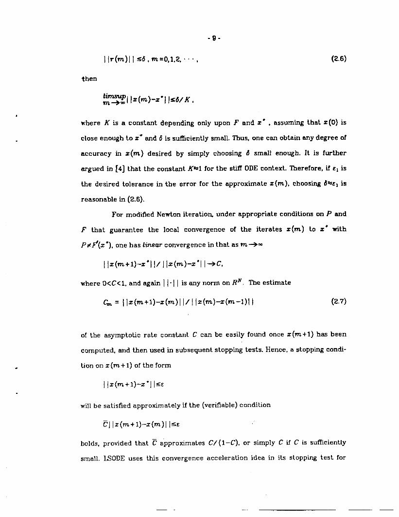
IIr(m)] I sxl, m=0,1,2, . . . . (2.6)

.

.

.

then

ti?nsup,m+=

n.here K is a c

z(m) -z”~JSd/K,

onstant depending only upon F and z” , assum-ing that z(0) is

close enough to z“ and d is sufficiently small. Thus, one can obtain any degree of

accuracy in z(m) desired by simply choosing 6 small enough. It is further

argued in [4] that the constant J@l for the stii ODE context. Therefore, if c1 is

the desired tolerance in the error for the approximate z(m), choosing tkl is

reasonable in (2.6).

For modified Newton iteratiom under appropriate conditions on P and

F that guarantee the local convergence of the iterates z(m) to z“ with

P#~(z “), one has linear convergence in that as m+=

llz(rn+l)-z”] l/]lz(m)-z”ll+C,

where O<C<l, and again I I.] I is any norm on RN. The estimate

G = {lz(m+O-z(m)l l/l lz(m)-z(m-1)1 I (2.7)

of the asymptotic rate constant C can be easily found once z (m + 1) has been

computed, and then used in subsequent stopping tests. Hence, a stopping condi-

tion on z (m + 1) of the form

Ilz(m+l)-z”]l<c

will be satisfied approximately if the (verifiable) condition

E] Iz(?n+l)-z(m)l ISE

holds, provided that ~ approximates C/(1 –C), or simply C if C is sufficiently

small. LSODE uses this convergence acceleration idea in its stopping test for

.- -.

-1o-

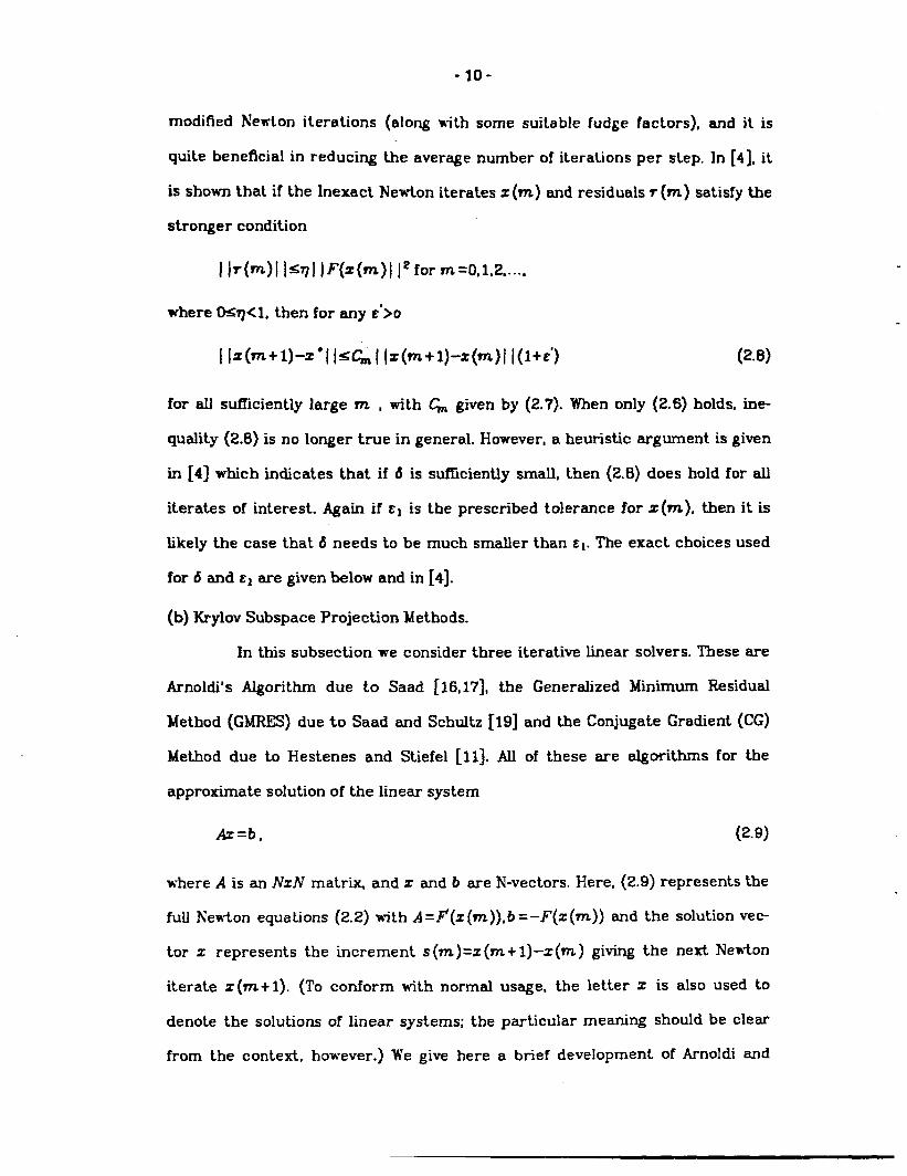
modified A’ewton iterations (along with some suitable fudge factors), and it is

quite beneficial in reducing the average number of iterations per step. In [4], it

is shown that if the Inexact Newton iterates z(m) and residuals r(m) satisfy the

stronger condition

~]r(m)] I$q] JF(z(rn.)] lzform=0,1,2,...,

where CMq<1, then for any C*>O

I lz(m+l)-z”ll<C&l Iz(m+l)-z(m)l I(l+t”) (2.B)

for all stiiciently large m , with & given by (2.7). When only {2.6) holds, ine-

quahty (2.B) is no longer true in general. However, a heuristic argument is given

in [4] which indicates that if 6 is sufficiently small, then (2.8) does hold for all

iterates of int crest. Again if c1 is the prescribed tolerance for z(m), then it is

likely the case that 6 needs to be much smaller than cl. The exact choices used

for 6 and c1 are given below and in [4].

(b) Krylov Subspace Projection Methods.

In this subsection we consider three iterative liear solvers. These are

Arnoldi’s Algorithm due to Saad [16,17], the Generalized khnimurn Residual

Method (GMRES) due to Saad and Schultz [19] and the Conjugate Gradient (CG)

Method due to Hestenes and Stiefel [11]. All of these are algorithms for the

approximate solution of the linear system

Az=b, (2.9)

where A is an NzN matr~ and z and b are N-vectors. Here, (2.9) represents the

full Newton equations (2.2) with A =~(z (m)),b = –F(z (m)) and the solution vec-

tor z represents the increment s (m)=z (m + 1)-z(m ) giving the next Newton

iterate z (m+ 1). (To conform with normal usage, the letter z is also used to

denote the solutions of linear systems; the particular meaning should be clear

from the context, however.) We give here a brief development of Arnoldl and

-11-

1

.

.

.

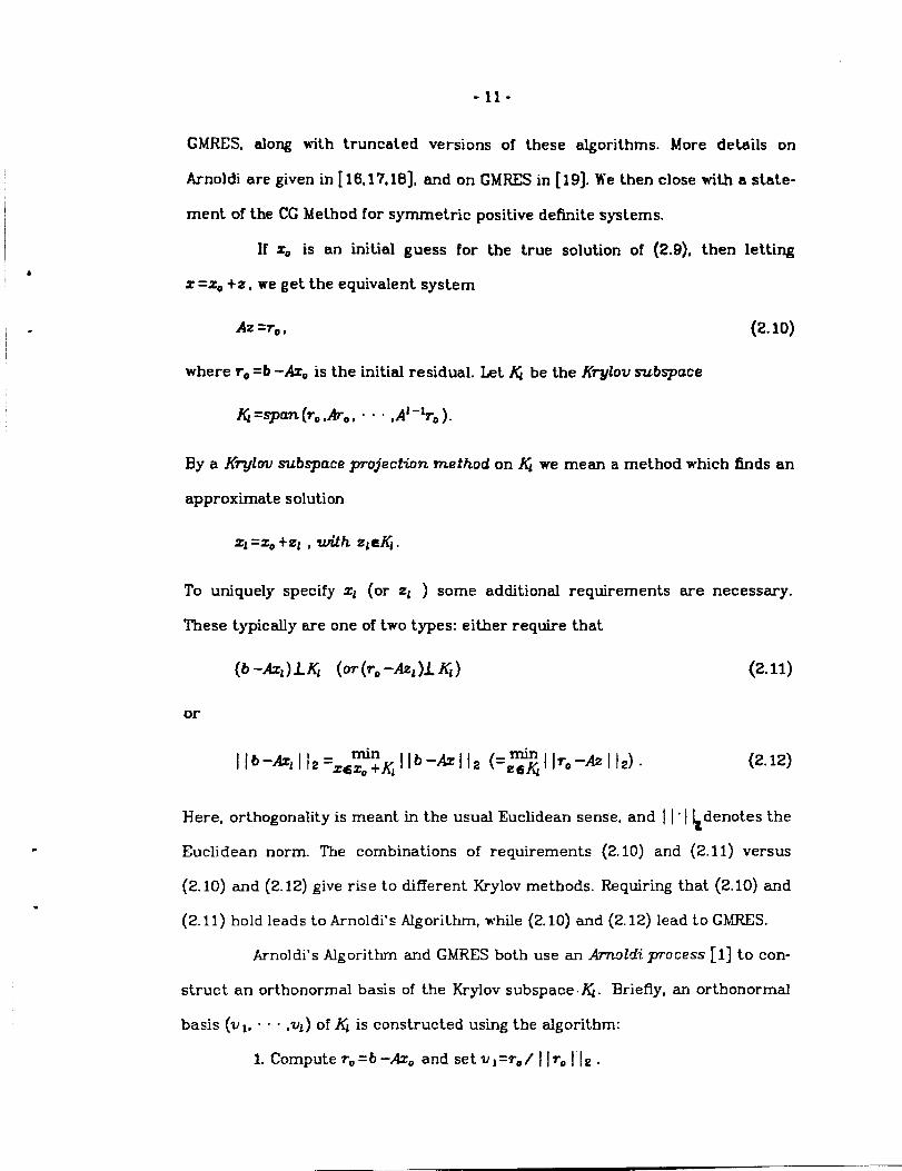
GMRES, along with truncated versions of these algorithms. More details on

Arnoldi are given in [ 16,17, 18], and on GMRES in [19]. We then close with a statem-

ent of the CC Method for symmetric positive definite systems.

If z. is an initial guess for the true solution of (2.9), then letting

z =ZO+Z, we get the equivalent system

Az =ro , (2.10)

where rc =b -AzO is the init,i~ residual. L& & be the &@ov subspzce

&=vun(ro,Aro, ‘ “ “ ,A1-lTO).

By a Kqlov subs-pace projection method on K we mean a method ~rhlch finds an

approximate solution

To uniquely specify ZL (or Z~ ) some additional requirements are necessary.

These typically are one of two types: either require that

@ -Azl)l& (or(r, -Azl)l. ~) (2.11)

or

(2. 12)

Here, orthogonality is meant in the usual Euclidean sense, and I I” I Ldenotes the

Euclidean norm. The combinations of requirements (2.10) and (2.11) versus

(2. 10) and (2. 12) give rise to different Krylov methods. Requiring that (2.10) and

(2. 11) hold leads to Arnoldi’s Algorithm, while (2.10) and (2.12) lead to GMRES.

Arnoldi’s Algorithm and GMRES both use an Arrdcii process [1] to con-

struct an orthonormal basis of the Krylov subspace &. Briefly, an orthonormal

basis (vl, - - 0,Vl) of K1 is constructed using the algorithm:

1. Compute TO=b–Azo andsetvl=70/ll~c!!z.

-12-

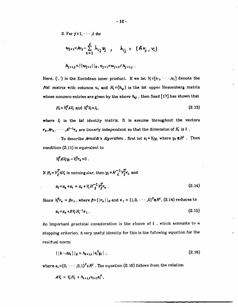
2. Forj=l, “ “ .,f do

Here, (“,”)

~+,=~j- ill ~,j’!) J1ij = [~vj , Vi)i=l

~,+1~=1 Iwj+ll 12 cuj+l=wj+I~q+lJ” .

is the Euclidean inner product. lf we let M=[v 1, - “ . ,wl] denote the

JVzl matrix with columns vi and fl~=(~) is the Lzl upper Hessenberg matrix

whose nonzero entries are given by the above ~ , then Saad [17] has shown that

where Xl is the lzl identity matrix. It

ro,Are, “ “ “ ,A1”%O are linearly independent

To describe Anzoltfi’s Algorithm ,

condition (2. 11) is equivalent to

(2.13)

is assume throughout the vectors

so that the dimension of & is t .

first let Z1= fiyl mThereVl CR1 . Then

If Hl = V~Alj is nonsingular, then yl =@ $’0 and

ZJ=Zo +21 Ifl= Zo+Jf Fl ~ro . (2. 14)

Since Jf%e = ~el , where $= I]r, ] 12and e ~ = (1,0, “ “ “ .O)T@, (2.14) reduces to

Z1=Za +~fi~l-le 1. (2.X5)

An important practical consideration is the choice of 1 , which amounts to a

stopping criteriom A very useful identity for this is the following equavlon for the

residual nornx

llb-Az1]12=~+l~je/yll ,

where ei =(0, - . “ ,0, l)TcR~ . The equation (2. 16) follows from the relation

(2.16)

Alj = &l?l + hl+lalvL+lelT,

●

.

.

-13-

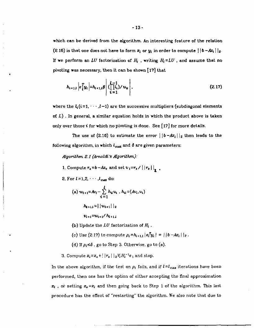
which can be derived from the algorithm. An interesting feature of

(2. 16) is that one does not have to form ZI or y~ in order to compute

the relation

llb-Azl 112.

If we perform an LU factorization of Hi , writing l?t =LU , and assume that no

pivoting was necessary, then it can be shown [17] that

h+l.1 $Yl h‘hl+LIP ( -t)/uu ,i=l

(2. 17)

where the ~(i=l, e “ . ,1-1) are the successive multipliers (subdiagonal elements

of L) . In general, a similar equation holds in which the product above is taken

only over those i for whlcb no pivoting is done. See [17] for more details.

The use of (2.16) to estimate the error 11b -Azl [ ]~ then leads to the

following algorithm, in which 1- and 6 are given parameters:

AlgonNun 2.1 (ArnoMi k Algorilh.m):

1. Compute ro=b–Azo and set v ~=r, / I jr. I ]? ,

2. For 1=1,2, - “ .,1- do

(a) W~+*=AV~-$ ~U~ , ~=(AIJL,U~)<=1

h+l.1=1 Iw+ll 12

vl+~=u)l+/b+~J

(b) Update the LU factorization of Hi .

(c) Use (2.17) to compute pl=~+let le/’yt I = I lb -Azl I Iz .

(d) If p~d, go to Step 3. Otherwise, go to (a)..

3. Compute Z1=ZO+ I Iro I I21jH1-le ~and stop.

In the above algorithm, if the test on p~ fails, and if 1=lW iterations have been

performed, then one has the option of either accepting the final approximation

21 , oi- setting 20 =Zl and then going back to Step 1 of the algorithm. This last

procedure has the effect of “restarting” the algorithm. M-ealso note that due to

-14-

the upper Hessenberg form of Fll there is a convenient way to perform an LU

factorization of HJ by using the LU factors of H, .l(l > 1) .

In Algorithm 2.10 as 1 gets large, a considerable amount of the work

involved is in makhg the vector U1,1 orthogonal to all the previous vectors

v~, ”’”,vl. Saad [17] has proposed a modification of Algorithm 2.1 in which the

vector VL+1 is only required to be orthogonal to the previous p vectors,

V1*+I, “ “ - ,Vl . Saad [17] has shown that equations (2.16) and (2. 17) still hold in

this case. This leads to an algorithm called the hcon@eie Whogorudizutbn

Method, denoted by 10M. It differs from Algorithm 2.1 ordy in that the sum in

Step 2(a) begins at i=% instead of at i=l . where & =max(l,z ~ +1) . The

remarks made after Algorithm 2.1 are also applicable to IOM. In [17], Saad com-

pares the two algorithms on several test problems, and reports that IOM is

sometimes perferred, based on total work required and run times.

When A is symmetric, the inner products ~,1 theoretically vanish for

i<l -1, so that one can take p =2 . If A is also positive definite then 10M withp =2

is equivalent to the Conjugate Gradient method [17, Sec. 3.3.1, Remark 4]. Thus

a value of p less than 1- might be expected to be cost-effective when A is

nearly symmetric.

Saad [17] and Gear and Saad [9] have given a convergence analysis of

Algorithm 2.1 which shows that Arnoldi’s Method converges in at most IV itera-

tions and suggests (but in general does not prove) that the convergence of the

iterates { ZI ] to the solutl,on of (2.9) is fastest in the dominant subspace (that is,

in those components corresponding to the eigenvalues in the outermost part of

the spectrum of A ), which would include the stiff components for the ODE con-

text.

The possibility of a breakdown also exists when using Algorithm 2.1.

This can happen in two different ways: either WI+1=0 so that vi +1 cannot be

.

.

formed, or ~JRUU

Arnoldi steps has

-15-

may be singular which means that the maximum number of

been take~ but the final iterate cannot be computed. The first

case has been referred to as a happy breakdown, since wt+l=O implies H1 is non-

singular and zl is the exact solution of (2.9) (cf. Brown [2] or Saad [18]). ‘he

second case is more serious in that it causes a convergence failure. In the ODE

setthg, where A= l-h/30 J , a way to handle the second failure is to reduce the

stepsize h and retry the step. We note, however, thk second kind of breakdown

cannot happen when A is positive definite. To see this, recall that HJ= WA If , and

so for any V#O

since Ify # O by the fact that If has orthonormal col,umns, and since A is positive

definite. Thus, HL is positive definite and so nonsingular.

The GMRES method differs from Arnoldi’s method only in the way the

vector yl is computed, WrhereZ1=ZO+ v yl . Suppose we have taken 1 steps of the

above Arnoldi process with w +1#O. Then we have two matrices,

~+, = [v,, .- s ,I++l]eR*f’+ll

whose columns are orthonormal, and the matrix El 6R[*+ 1)* defined by

It follows from the Arnoldi process that

Afi=lj+l~i .

The vector Ztefi is chosen to satisfy (2.12), namely

I l~o-Az~112=Z~&l ]TO-AZ] 12.

(2.18)

(2.19)

-16-

letting z = Ijy and using (2. 18) gives

J(~)=llrO-AZ I Iz=I l@l-AJjyl (z

=l]lf+j(j3e1-R~y)l ]R=I lpe~-~lyl 1~

where #=]]ro] 12, el=(l,O, . “ “ ,O)TeR[+l, since fi+l has mt.honormal columns.

Thus, the solution of (2. 12) or (2.19) is given by

zl=~ +lfyi ,

where yl minimizes J(v) over VeR1 .

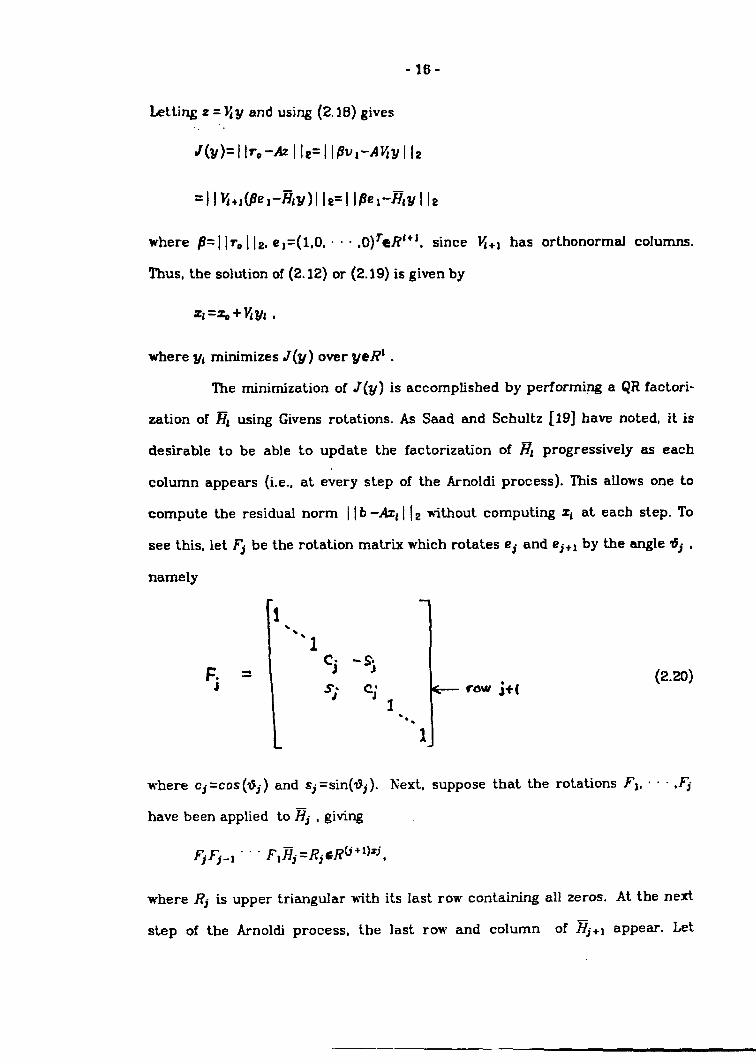
The minimization of ~(y) is accomplished by performing a QR factori-

zation of ~1 using Givens rotations. As Saad and Schultz [19] have noted, it is

desirable to be able to update the factorization of El progressively as each

column appears (i.e., at every step of the Arnoldl process). This allows one to

compute the residual norm IIb –Axl I Iz without computing Z1

see this, let Fj be the rotation matrix which rotates ej and ej +I

namely

F.J

where cj =COS(tj ) and sj =sin(Oj ).

have been applied to Rj , giving

Irew j+(1

‘.*

1

at each step. To

by the angle ~j ,

(2.20)

Next, suppose that the rotations ~1, c “ . .Fj

where Rj is upper triangular with its Iast row containing all Zeros. At the neti

step of the Arnoldi process, the last row and column of ~j+l aPPear. Let

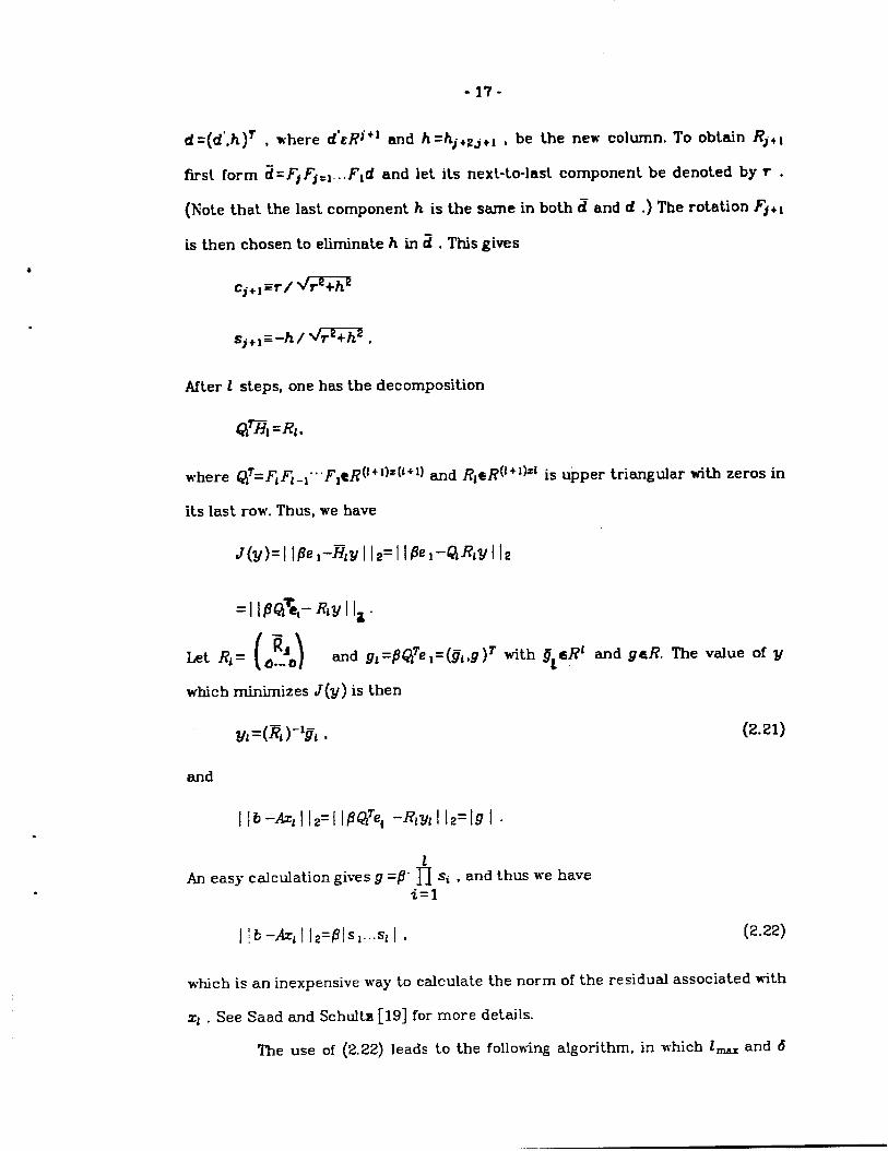
-17-

d =(d’,h)r , where d’tRJ+’ and h =hj+zj+l , be the new column. To obtain RJ+ 1

first form ~= FjFj.l... Fld and let its next-to-last component be denoted by r .

(Note that the last component h is the same in both ~ and d .) The rotation ~jti

is then chosen to eliminate h in ~ . This gives

cj+l~r/~

After 1 steps, one has the decomposition

Q%, =Rl ,

where QT=FIF’.l-”” ~1@+04 +0 and RleR~l ‘]~~ is upper triangular with zeros in

its last row. Thus, we have

J(v)=I l~el-~lyl 12=1 18el-QRvl 12

(2.21)

and

.

1h easy calculation gives g =8- ~ Sa , and thus ~’e have

i=l

I; L-AJI12=191S,...%1 , (2.22)

which is an inexpensive way to calculate the norm of the residual associated with

Z1 . See Saad and Schulta [19] for more details.

The use of (2.22) leads to the following algorithm, in which 1- and 6

-18-

are given parameters:

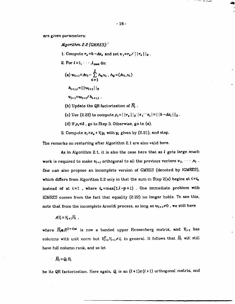
M~07ith~ 2.2 (GMRES);

1. Compute rO=b-Aza and setul=ro/ I Ire I {2 .

2. Forl=l, .” &X ~~

%+1=% +1/4+1,1 .

(b) Update the QR factorization of ~~ .

(c) Use(2.22) tocomputepl=l \rOl12`lsl"""sl l=llb-&lllz.

(d) If pl<d , go to Step 3. Otherwise, go to (a).

3. Compute z~=ZO+ ~yl withy, given by (2.21), and stop.

The remarks on restarting after Algorithm 2.1 are also valid here.

As in Algorithm 2.1, it is also the case here that as 1 gets large much

work is required to make q +1 orthogonal to all the previous vectors Vl, “ c . ,vl .

One can also propose an incomplete version of GMRES (denoted by IGMRES),

which differs from Algorithm 2.2 only in that the sum in Step 2(a) begins at ~=%

instead of at i =1 , where ~ =max(l,l ~ +1) . One immediate problem with

IGMRES comes from the fact that equality (2.22) no longer holds. To see this,

note that from the incomplete Arnoldi process, as long as WJ+1#0 t We Stfll h-

where ~ld?~l +*JA is now a banded upper Hessenberg matrix, and V+ I ha

columns with unit norm but ~+1 ~ +A#1~ in general. lt follows that ~~ will still

have full column rank, and so let

.

.

be its QR factorization. Here agai~ Q is an (t+ I)z(l + 1) orthogonal matrix and

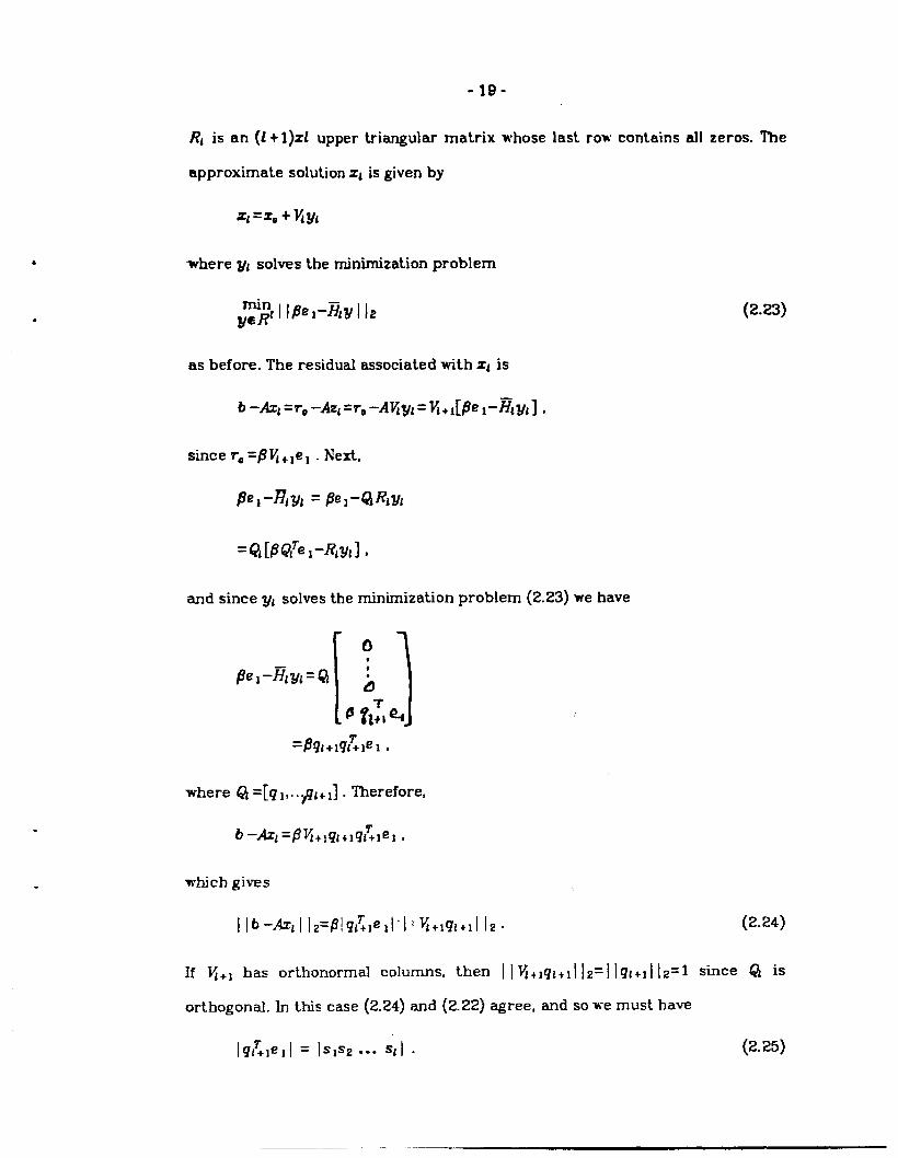
-19-

RI is an (1+ I)zl upper triangular matrix whose last row contains all zeros. The

approximate solution ZLis given by

where yl solves the minimization problem

(2.23)

as before. The residual associated with Z1 is

and since yl solves the rninimizatilon problem (2.23) we have

[1

o

~el-E?iyt=Q j

@flyl %

=P9~+lqiZlel.

where ~ =[q 1,.. .fll+1] . Therefore,

b–kl=plj+lql +lqi?lel ,

E v+] has orthonormal columns, then ] l~+lgl+lllz=l]ql+l]lz=l s~ce ~ is

orthogonal. In this case (2.24) and (2.22) agree, and so w-emust have

lq~lell = Islsz ,.. s~l . (2.25)

To show that (2.25) still holds when

require some further justification.

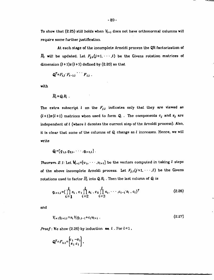
-20”

~+, does not have orthonormal columns will

At each stage of the incomplete Arnoldi process the QR factorization of

~, will be updated. Let ~,~(j=l, “ ~. ,1) be the Givens rotation matrices of

dimension (1+ l)z (1+ 1) defined by (2.20) so that

QT=%”FLIJ “ “ “ F,J .

with

The extra subscript 1 on the Fj,l indicates OnlY that they are Mewed as

(i +l)z(l +1) matrices when used to form Q . The components Cj and ~j are

independent of 1 (where 1 denotes the current step of the Arnoldl process). Also,

it is clew that some of the columns of ~ change as 1 increases. Hence, we will

write

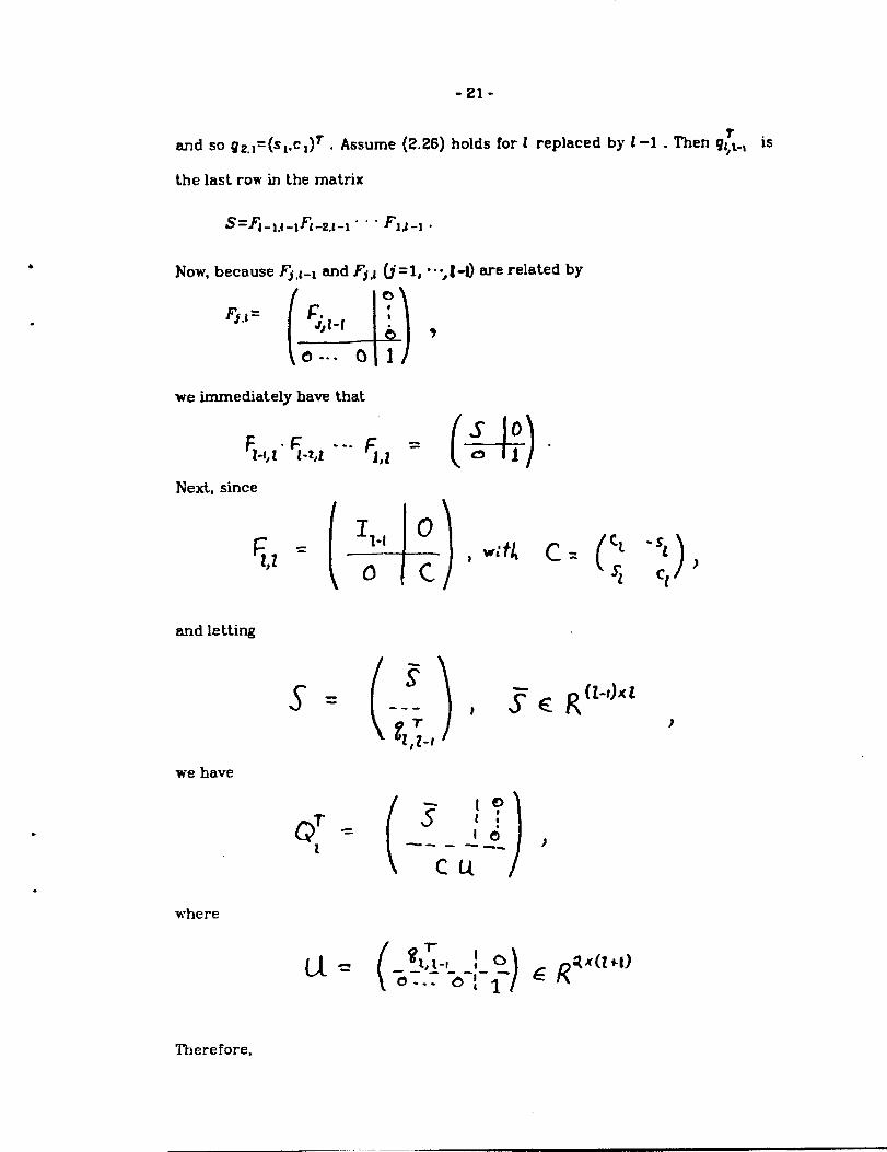
?9umrern 2.1: Let Vl+l=[vl, . “ “ .VI+I] be the vectors computed in taking 1 steps

.of the above incomplete Arnohi.i process. Let Fj.t (j = 1, 0 c “ ,t ) be the Givens

rotations used to factor ~~ into Q R1 . Then the last column of ~ is

1 1 i91+1.t=(IISi . cl~% . C2~ %, “ “ ‘ ,Ct-l”S~ , Cl)T

~=1 i=2 ‘i=3

and

If+,gl+l.l=sl lfql,l_~+clvl+l .

&oo/: %-e show (2.26) by induction on 1. For 2= 1.

(2.27)

.

(2.26)

-21-

and SO gz.l=(~l,ct) T . Assume (2.26) holds for 1 replaced by I-1 . Then ft., is

the last row in the matrix

Now, because ~j.t-l and Fj,l ~ ‘l, ‘ - ;t-~ We related b’

F$.l=

(-4-4

r, ‘?J, I-l . ?

6 -. . 01

we immediately have that

Next, since

and letting

s H9= --- J ~ pdxt

t?T ‘1,2-I

we have

where

u‘(

%T:ot, t-l

)=R

~x(l+l)—___ . . .0 --- 6{1

Therefore,

)

—..

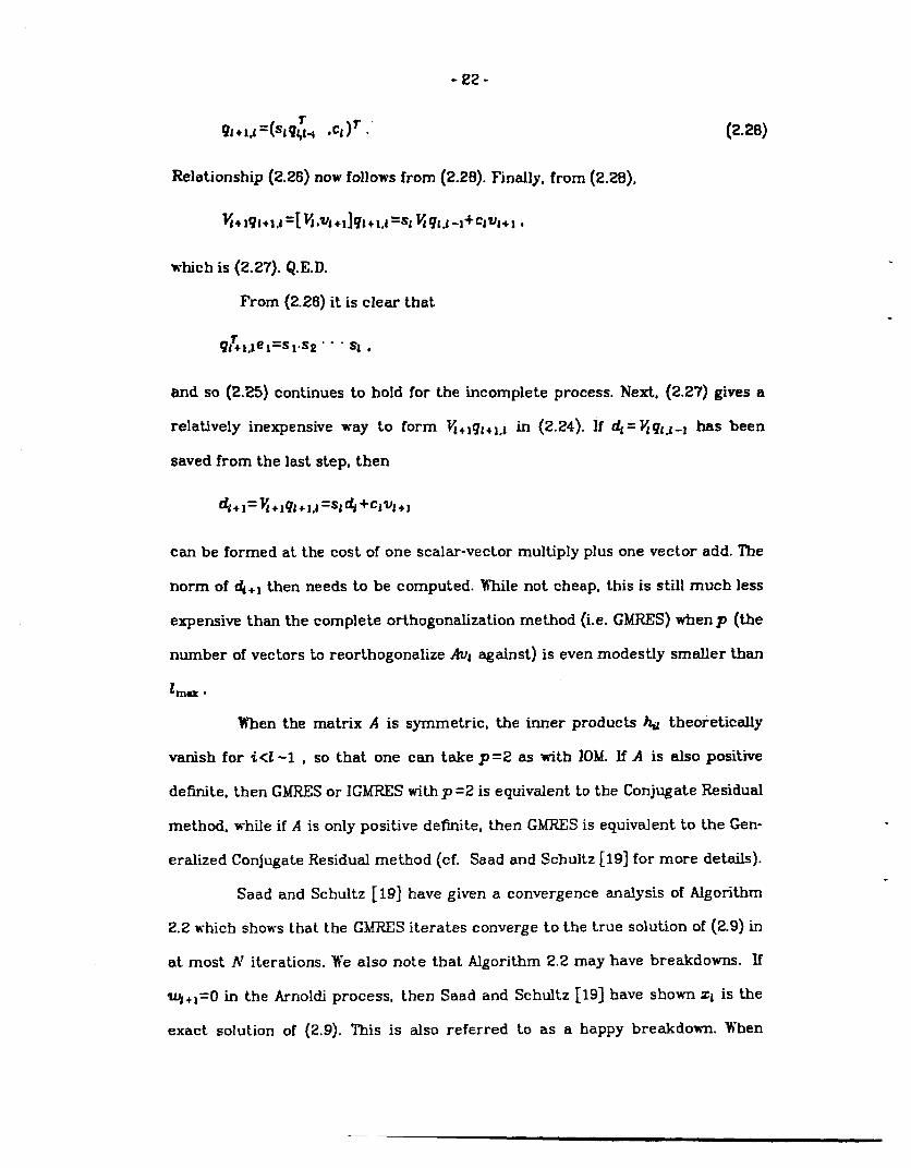
91+1J=(W;.I X[)r .’ (2.20)

Relationship (2.26) now follonrs from (2.29). Finally, from (2.28),

which is (2.27). Q.E.D.

From (2.26) it is clear that

9T+l.lel=sl.s2 .”” S1,

and so (2.25) continues to hold for the incomplete process. Next, (2.27) gives a

relatively inexpensive way to form Tf+lgl+l,l in (2.24). If dl = JfqfJ_l has been

saved from the last step, then

can be formed at the cost of one scalar-vector multiply plus one vector add. ‘l%e

norm of ~ +1 then needs to be computed. While not cheap, this is still much less

expensive than the complete orthogonalization method (i.e. GMRES) when p (the

number of vectors to reorthogonalize Avl against) is even modestly smaller than

1ma .

When the matrix A is symmetric, the inner products k theoretically

vanish for i <1-1 , so that one can take A =2 as with IOM. If A is also positiie

definite, then GMRESor IGMRES with p =2 is equivalent to the Conjugate Residual

method, while if A is only positive defilte, then GMRES is equivalent to the Gen-

eralized Conjugate Residual method (cf. Saad and Schultz [19] for more details).

Saad and Schultz [19] have given a convergence analysis of Algorithm

2.2! ~-hich shows that the GMRES iterates converge to the true solution of (2.9) in

at most A’ iterations. We aIso note that Algorithm 2.2 may have breakdowns. If

Wt+l=t) in the Arno]til process, then Saad and Schultz [19] have shown Z1 is the

exact solution of (2.9). This is also referred to as a happy breakdown. When

-23-

.

.

.

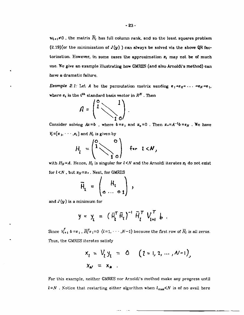
WJ+1#O , the matrix El has full column rank, and so the least squares problem

(2.19) (or the minimization of J(y) ) can always be solved via the above QR fac-

torization. However, in some cases the approximation zl may not be of much

use. We give an example illustrating how GMRES (and also Arnoldi’s method) can

have a dramatic failure.

Ezumple 2.1.’ Let A be the permutation matrix sending e ,+ez+ . . . ~eN~e,,

where ei is the i;~ standard basis vector in RN . Then

(\)c) 1

A=l.\ lo

Consider solving Az=b , where b =e ~ and ZO=0 . Then z.=A-lb =e~ . We have

with Hx =A. Hence, HL is singular for 1<A7 and the A.rnoldi iterates Z1 do not exist

for 1<N , but zN=~. . Next, for GMRES

and J(y) is a minimum for

Since /+1 b=el, E~el=O (1=1, . “ “ ,N–1) because the fhst row of El is all zeros.

Thus, the GMRES iterates satisfy

xl = yyl = d (2= 1,2, . . .. A+.

xv =X*.

For this example, neither GMRES nor Arnoldi’s method make any progress until

2=N . Notice that restarting either algorithm when lW<N is of no avail here

-----”-y-24-

either.

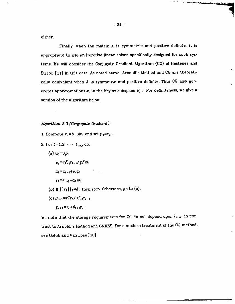
Finally, when the matrix A is symmetric and positive definite, it is

appropriate to use an iterative linear solver specifically designed for such sys-

tems. We will consider the Conjugate Gradient Algorithm (CG) of Hestenes and

Stiefel [11] in this case. As noted above, Arnoldi’s Method and CG are theoreti-

cally equivalent when A is symmetric and positive defhite. Thus CC also gen-

erates approximations Z1 in the Krylov subspace KI . For definiteness, we give a

version of the algorithm below.

Algo7Wun 2.3 (Conjugate &adien.1):

1. Compute rO=6 -Azo and set pl=ro .

2. Forl=l,2, . c . ,1-do

(a) w, =Ap~

Q=r~,r,-#p@l

zl=zl_]+~pl “

Ti=Ti .I-oqwl

(b) k i \r~I l#d , then stop. Otherwise, go to (c).

(c) /%+1‘@rl/ ~Ll~l-1

Pi+l=rl+Pl+@l .

We note that the storage requirements for CG do not depend upon l-, in con-

trast to Arnokli’s Method and GMRES.For a modern treatment of the CG method,

see Golub and Van Loan [10].

.

.

.

-25-

*

.

.

.

3. flon.linear Convergence Z%eory

For all of the algorithms considered in Sec. 2(b) the matrix A is not needed

explicitly. All one needs is to be able to calculate matrix-vector products of the

form Av , for v any vector. %ce A=7(Z) for Z an approximation to a root of

(2. 1), the matrix-vector products Av in the above algorithms can be replaced by

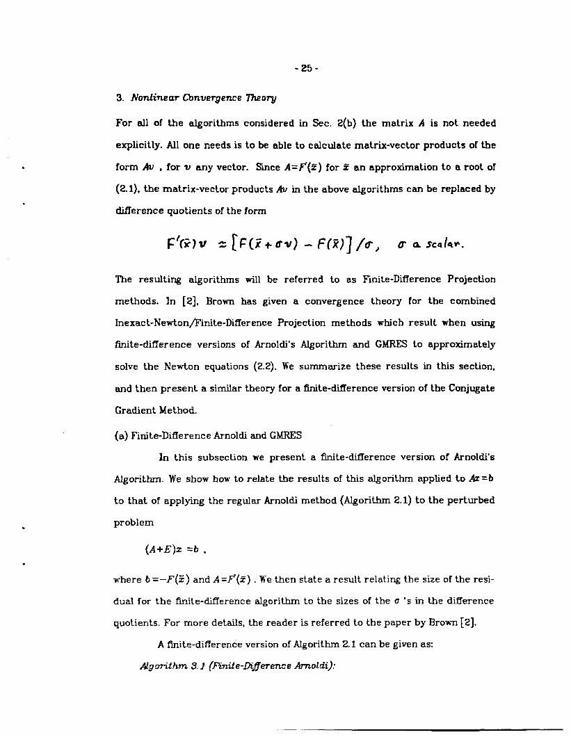
difference quotients of the form

The resulting algorithms will be referred to as Fhite-Difference Projection

methods. In [2], Brown has given a convergence theory for the combmed

Inexact-Newton/l?inite-Difference Projection methods which result when using

finite-difference versions of Arnoldi’s Algorithm and GMRES to approximately

solve the h’ewton equations (2.2). We summarize these results in this section,

and then present a similar theory for a f?mite-dMference version of the Conjugate

Gradient Method.

(a) Finite-llifference Arnoldi and GMRES

In this subsection we present a fite-difference version of Arnoldi’s

Algorithm. We show how to relate the results of this algorithm applied to AZ=b

to that of applying the regular Arnoldi method {Algorithm 2.1) to the perturbed

problem

(A+E)z =b ,

where b =–F(5) and A =~(it)

dual for the f?mite-di.fference

. We then state a result relating the size of the resi-

algorithm to the sizes of the o ‘s in the difference

quotients. For more details, the reader is referred to the paper by Bromm[2].

A finite-difference version of Algorithm 2.1 can be given as

AQcmithm 3.1 (finiie-Di’erence Amoldi,):

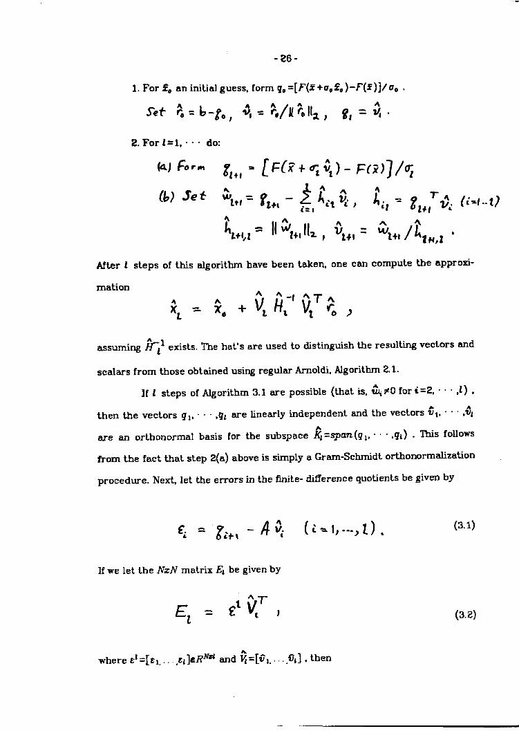
t,+, ~ =/

After 1 steps of this algorithm have

matlon A

?L = ;6 + v’

been taken, one can compute the approxi-

assuming %11 exists. The hat.’s are used to disthguish the resulting vectors and

scalars from those obtained using regular Arnoldl, Algorithm 2.1.

lf 1 steps of Algorithm 3.1 are possible (that is, & #O for ~=2, - “ - ,1) ,

then the vectors gl, - . - ,gl are linearly independent and the vectors 61, “ o “ ,$

are an orthonormal basis for the sub space k =spa7z(gl, c . “ ,gl) . This follows

from the fact that step 2(a) above is simply a Gram-Schmidt orthonorrmdization

procedure. Next, let the errors in the finite- difference quotients be given by

4f~=-;i r(w)-- .)l).z+t

If we let the A’zlV matrix El be given by

(3.1)

(3.2)

.

.

(3.3)

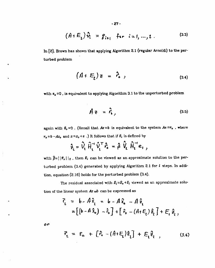
In [2], Brown has shown that applying Algorithm 2.1 (regular Arnoldi) to the per-

turbed problem

with ZO=0, is equivalent to applying Algorithm

(3.4)

3.1 to the unperturbed problem

k? -- ~, (3.5)

again with 20=0 . (Recall that AZ =b is equivalent to the system Az =rO , where

TO=b -Azo and z =ZO+Z .) R follows that if gl is defied by

]FOI I~ , then S, can be viewed as MI approximate solution to tie Per-

roblem (3.4) generated by applying Algorithm 2.1 for 1 steps. In addi-

tion, equation (2. 16) holds for the perturbed problem (3.4).

The residual associated with S1=20 +21 viewed as an approximate solu-

tion of the linear system AZ =b can be expressed as

(3.6)

-26-

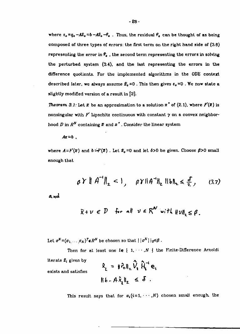
where to =qO-A!& =b -/@O 40 . Thus, the residual fO can be thought of as being

composed of three types of errors: the first term on the right hand side of (3.6)

representing the error in Fe , the second term represent@ the errors in solving

the perturbed system (3.4), and the last representii the errors in the

difference quotients. For the implemented algorithms in the ODE context

described later, we always assume E. =0 . This then gives CO=0 . We now state a

slightly modtied version of a result in [2].

7heorsm 3.1: Let Z be an approximation to a solution z ● of (2.1), where ~(=) is

nonsingular with F’ LipschNz continuous with constant y on a convex neighbor-

hood D in l?~ containing Z and z” . Consider the linear system

Az=b ,

where A =F’(Z) and b =~(z) . Let $0 =0 and let d>O be given. Choose (?>0 small

enough that

Let d=(ul.. . . ,uN)TeRN be chosen so that I Idl ]~~ .

Then for at least one le [ 1, e . c ,N ] the Ftite-Difference Arnoldi

This result says that for Ui(i= 1, “ . “ N) chosen sm~l enow4 the

-29-

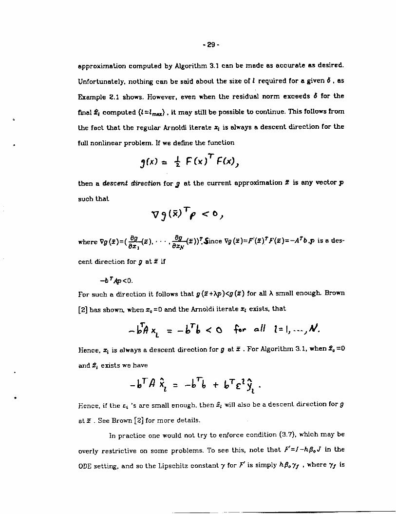
approximation computed by Algorithm 3.1 can be made as accurate as desired.

Unfortunately, nothing can be said about the size of 1 required for a given 6, as

Example 2,1 shows. However, even when the residual norm exceeds d for the

final @i computed (1=1-) , it may still be possible to continue. ‘fMs follows from

the fact that the regular Arnoldi iterate z~ is always a descent dkection for the

full nonliear problem. If we define the function

then a desce’nl direction for g at the current approximation Z is any vector p

such that

vj(@p <0,

cent direction for 9 at Z if

–b~Ap<o.

For such a direction it follows that g (5 +Ap)<g (5) for all A small enough. Brown

[2] has sho~ when z. =0 and the Arnoldl iterate Z1 exists, that

- LTAXL = -Lrb <0 for ail Z= I, .--, #.

Hence, zl is always a descent direction for g at Z . For Algorithm 3.1, when&=0

and Ei exists we have

Hence, if the &i ‘s are small enough, then 51 will also be a descent direction for g

at 5 . See Brown [2] for more details.

In practice one would not try to enforce condition (3.7), which may be

overly restrictive on some problems. To see this, note that ~=1 –h~o J in the

ODE setting, and so the Llpschitz constant y for ~ is simply h#%YJ , where 73 is

the Lipschitz constant fordJ/&?y ,

problem yl can be quite large, and

in too small a value of h . This is

-30-

the ODE system Jacobian. For a typical stiff

so trying to force (3.7) to bold would result

the price one pays for using norms in the

analysis as the Lipschltz constant 7 measures the worst-case nonlinearity in F .

A better approach is to choose the ui so that the errors in the fl.nite-dlflerence

quotients are small. See Brown [z] for more details, and Dennis and Schabel [7]

for more general information on computing finite-difference derivative approxi-

mations. Since Arnoldl and GMRES both use the same Arnoldi process, a com-

pletely sirnWw theory is true for the finite-difference version of GMRES.We refer

the reader to [2] for more details.

(b) Finite-Difference Conjugate Gradient

in [2], Brown has presented a convergence theory for a finite-difference

version of the Generdlzed Conjugate Residual method of Eisenstat, Elman and

Schultz [8]. Here, we show how a mo~cation of thk theory will allow us to prove

a result similar to Theorem 3.1 for a !3nNe-dmerence version of the Conjugate

Gradient Method. The main tool will again relate the results of the finite-

difference algorithm to that of applying the regular algorithm to a perturbed

problem

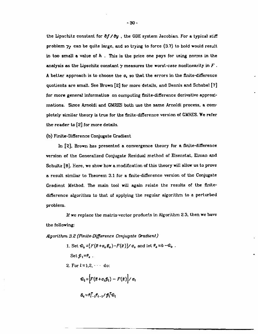
If we replace the matrix-vector products in Algorithm 2.3, then we have

the following:

AZgm-ifhm 3.2 (Fintie-Difleren.ce Conjugate &adia?nf)

1. Set 00 =[F(Z+uOfO )-F(z)]/ UOand let fO=b -fDO .

Setj31=F0 .

2. For 1=1,2, “ . “ do:

al= ~(z+u,pl) - F(z)]/ u,

& =P:_iFt_l/&@

.

-31-

.

.

.

.

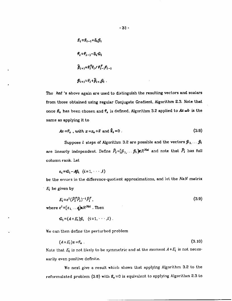
‘l’he haf *s above again are used to distinguish the resulting vectors and scalars

from those obtained using regular Conjugate Gradient, Algorithm 2.3. Note that

once !?O has been chosen and FOis defined, Algorithm 3.2 applied to AZ =b is the

same as applying it to

AZ=FO ,tihz=zO+k%nd~O=O. (3.0)

Suppose 1 steps of Algorithm 3.2 are possible and the vectors Z ~. ~1

are linearly independent. Define ~1=~l,. . . @~l@’d and note that ~1 has full

column rank. Let

&i=@–@ (i=l. ‘ - “ .1)

be the errors in the difference-quotient approximations, and let the ~zN matrix

El be given by

El =&z(P~F~)-1P: , (3.9)

where cl =[2,,.. .@?&’. Then

*=(~+G)fii (~=1, “ -- ,1) .

We can then define the perturbed problem

(A+ E~)z=Fo . (3.10)

Note that Ei is not likely to be symmetric and at the moment A +El is not neces-

sarily even positive definite.

We next give a result which shows that applying Algorithm 3.2 to the

reformulated problem (3.8) with !20=0 is equivalent to applying Algorithm 2.3 to

-- . - -. ..._ti -,_

-32-

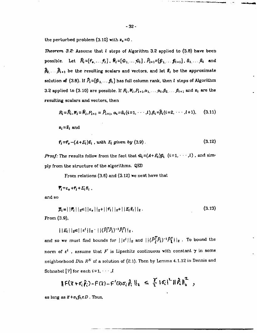
the perturbed problem (3. 10) with z, =0 ,

7Aeorem 3.2: Assume that 1 steps of Algorithm 3.2 applied to (3.8) have been

possible. Let ~l=[f,o.. .,FI] , @l=[til,...,ti, ], ~~+l=~l,... ~1+1], Eil. . ...& and

?2,... ,Bt+l be the resulting scalars and vectors, and let !?~ be the approximate

solution * (3.8). If PI=@l... , j$ ] has full coh.unn rank, then 1 steps of Algorithm

3.2 applied to (3.10) are possible. If RI. W’l,Pl+l,al,. . . ,at,j?12m. . . ./$+l and ZI are the

resulting scalars and vectors, then

R1=~l, Wl=@l,P1+l = Fl+l, ai=ai(i=l, “ “ “ ,l),@i=&(i=2, “ “ “ ,1+1), (3.11)

Zq=21 and

F1=FO–(A +El )~1 , wifh E“ given by (3.9) . (3. 12)

fioo~: The results follow from the fact that ~ =(A+& )fi (i=l, “ o “ ,1) , and sim-

ply from the structure of the algorithms. QED

From relations (3.6) and (3. 12) we next have that

~=c@+91+El

and SO

Ih=llfill+

From (3.9),

(3.13)

llElll#lle’\12” H(Fm-’RTH2t

and so we must find bounds for j IZ1I]2 and I ! (~~~1 )-*~{ I I2 . TO bound the

norm of Et , assume that ~ is Lipschltz continuous with constant y in some

neighborhood Din Rhr of a solution of (2. 1). Then by Lemma 4.1.12 in Dennis and

Schnabel [7] for each z=l, ‘ . “ ,1

ift~+ri~i~-f(z)-f’(firi~i \lz z ~ hfilhlh~ ~

as long as E +uifii~D . Thus,

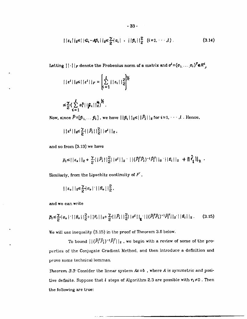
-33-

ll&i112<i lQ-@ill#~ui/ ● ll$ill~ (i=l, “- “,/). (3.14)

Letting I I. I I~ denote the Frobenius norm of a matrix and ~ =(ul, . . . ,uL)rcR\

.

and so from (3.13) we have

Similarly, from the Lipschitz continuity of F“,

and we can write

.

.

We will use inequality (3. 15) in the proof of Theorem 3.6 below.

To bound IJ(~~~1 )-1~1~1Iz , we begin with a review of some of the pro-

perties of the Conjugate Gradient Method, and then introduce a definition and

prove some technical lemmas.

7$worern 3,3: Consider the linear system AZ =h , where A is symmetric and posi-

tive definite. Suppose that 1 steps of Algorithm 2.3 are possible with rl #O . Then

the following are true:

-34-

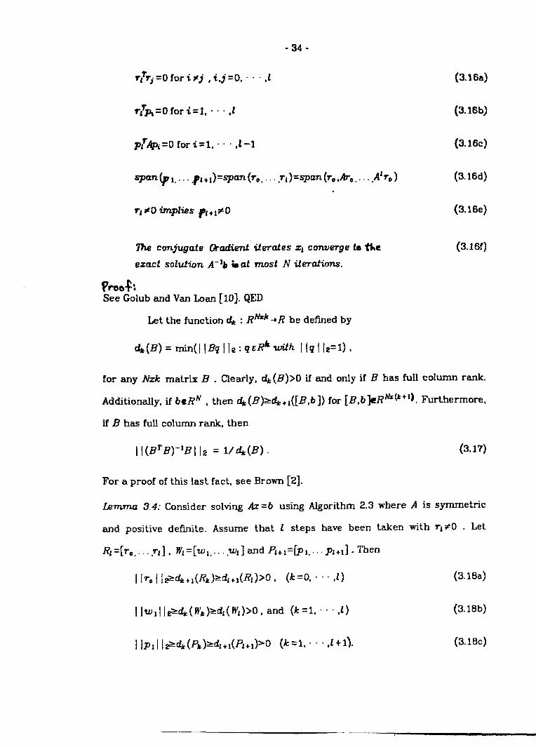
rlTrj=Dfor i#) , i,j=O, . “ “ ,! (3.16a)

r’/’&=Ofori=l, “ “ . ,i (3.16b)

PT@i=Ofori=l, . ...1-1 (3.16c)

Va~(pL... .p++qu~(ro,... ,Ti)=qpan(ro,fio,...,AITO) (3.16d)

rl#O implies ~1+1#0 (3.16e)

7he conjugate fhdient itercdes q converge ta Se (3.16f)

ezucf solutimt A“ib k at most N iterations.

?r’oef:See Golub and Van Loan [10]. QED

Let the function ~ : R~ +R be defined by

for any Nzk matrix B . Clearly, d~(B)>O if and only if 13 has full column rank.

Additionally, if &eRN , then A (l?)> ~+l([13,b ]) for [l?,b ld?k@+ll, Furthermore,

if 1? has full column rank, then

I l(~T~)-lBl I* = l/&(B) - (3.1?)

For a proof of this last fact, see Brown [2].

Lemma 3.4: Consider solving Az =b using Algorithm 2.3 where A is symmetric

and positive defilte. Assume that 1 steps have been taken with T1#O . Let

Rl=[ro.. . ..rl] , W’=[W1... .Wt] and PL+l=~l... .yl+l]. Then

I lr~ I l>dk+l(R~)~di+l(~~)>O , (k=O, ~~~,2) (3.18a)

llwllle>d~(~~)>dl(Wl)>O, and (k=l, ~. . ,1) (3.lEIb)

-35”

.

.

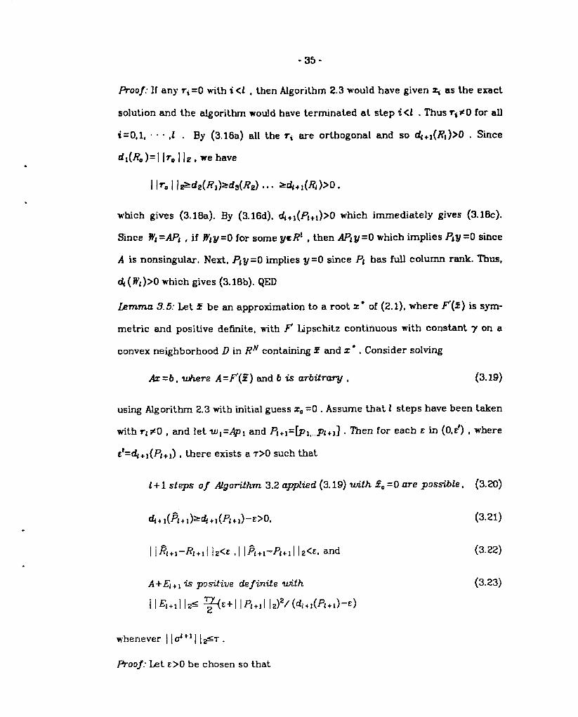
~oo~: If any ri =0 with i <1 , then Algorithm 2.3 would have given % as the exact

solution and the algorithm would have terminated at step ~<1 . Thus rj#O for aU

i=o,l, “ “ “ ,1 . By (3.16a) all the r8 are orthogonal and so dL+l(Rl )>0 . Since

cfl(RO)=~ Iro ] Iz , we have

11~. I l>d@,)~dg(Rz) t . . ~4+I(RL)>o s

which gives (3. 18a). By (3. 16d), cfl+l(F’~+l)>O which immediately gives (3. 16c).

Since B’t=APJ , if B’ly =0 for some VCR 1 , then APly =0 which implies Piy =0 s-mce

A is nonsingular. Next, Ply =0 implies y =0 since PI has full column rank. Thus,

~ (B’l)>O ~rhich gives (3.18b). QED

Lemma 3.5: Let z be an approximation to a root z” of (2. 1), where ~(z) is sym-

metric and positive definite, with F’ Epschitz conthiuous with constant 7 on a

convex neighborhood D in RN containing Z and z‘ . Consider solving

k =b, where A =1’.(E) and b * arbitrary , (3.19)

using Algorithm 2.3 with initial guess Z. =0 . Assume that 1 steps have been taken

with rl #O , and let W1=41 and Pl+l=(pl,..pt+l] . Then for each z h (flc’) t where

ct=~ +1(~~+1), ~ere efists a T>O such hat

l+ 1 steps of AlgorWwn 3.2 a~ied (3.19) tith & = O are possible, (3.20)

A +El. ~‘i-sp~tiive definite with (3.23)

~E+I IP,+,I 1,)2/ (dL+,(Pl+l)-&)l\&+ll 12= ~

w~benever I Iti+l I 1~~ .

pro~f: let .s>0 be chosen so that

..

-36-

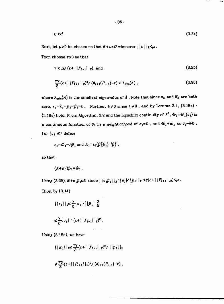
(3.24)c <c’ .

Next, let p>O be chosen so that z+veD whenever I Iv I I2<P .

Then choose 7>0 so that

7c@(E+l Ipt+ll Iz), and (3.25)

~c+l ]fi+ll lz)2/(ti,+,(Pl+,) -c) < Ati(A) , (3.26)

where ~(A) is the smallest eigenvdue of A . Note that since Z. and se are both

zero, To=FO=p I=fii=b. Further, b #O since rl #O , and by Lemma 3.4, (3.18a) -

(3.18c) hold. From Algorithm 3.2 and the Lipschitz continuity of ~, tiI=fil(oI) is

a continuous function of U1in a neighborhood of al= O , and @ l+u I as ol+o “

For IU1I<~ define

so that

(A+EJfi~=a~ .

Using (3.25), E +u@lcD since ]

ThUS,by (3. 14)

H%llsyull’llfilllg

<boll-(C+ II P1+,112)2.

Using (3. 1!3c), we have

llElll@~&+ llPl+l 112)’/

<&&+l Ifi+ll 12)2/(4+ Wt.

IPII 12

J-&) ,

-37-

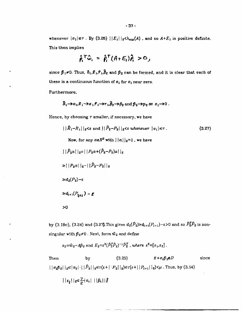
whenever lo] IST . By (3.26) I IEII lz<&(A) , and so A+El is positive de!inite.

This then implies

since ~1 *O. Thus, fil,~l,pl,~z and fiz can be formed, and it is clear that each of

these is a continuous function of al for al near zero.

Furthermore,

~l-al,~l-z I,f l+r 1,~2+#2 and fi2+p2 as UI+O .

Hence, by choosing T smaller, if necessary, we have

I

I

RI–RI I lz<& and JI~z-Pzl Iz<.Ewhenever Ial I<T.

Now, for any ael?zwit.h 1la] 12=1 , we have

(3.27)

>llP2a112-llP2-P21/2

‘ai@J-&

=J+l(p\+l ) - f

>0

by (3. 18c), (3.24) and (3.2’7). This gives d2(~2)ad1 +1(~~+1)-c>O and so ~1~2 is non-

singular with ~2#0 . Next, form fi2 and define

z2=@2–A.$2 and EZ=C2(~l~2)-*~i , where t2=[t1, cz] .

Then by (3.25) f+o&#D since

I lo~zl l~luzl.l 1~21 IZST(E+I IP21 ]Z)ST(C+I \Pl~ll l&P. Thus, by(3.14)

Hqll#&il IIAII:

. .. .. _____ . . . ____.. ..

-38-

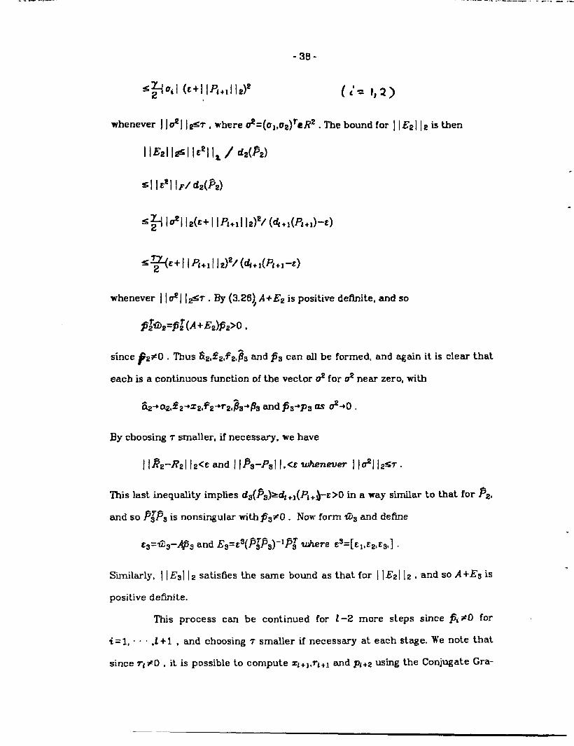
S~Uil (&+l IP,+,I 1~)’ (c’= 1)2)

whenever ] Id] I~? , where &=(01, U2)rGR2 . The bound for I

11~211#1 l&211 a/dz(P2)

= I I EZI IF/ ~2(A)

<~ IU21 Iz(c+ I Iq+ll 12)2/ (~+1(~1+1)-c)

=~c+l IPJ+l I li?)2/(4+AR+l-&)

2 is then

whenever I I& I l@ . By (3.261A +i72 is positive definite, and so

j5@2=p:(A+E&32>o ●

since t 2#0 . Thus ~2,2?2,F2,~gand ~9 can all be formed, and again it is clear that

each is a continuous function of the vector & for & near zero, with

F “ ~ +IIJgand j33”p3 as &+O s&+cQ,fpz2, 2 ~2* s

By choosing T smaller, if necessary. we have

I !~2-R2{ 12Q md ] l~g-l?sl 1,<E whenever

Thk last inequality implies dg(~9)>d1+l(P1+&&>0 in a way similar to that for ~2,

and so ~~~3 is nonsingular with fig#O . Now form fig and define

c3=Cg-Aj5g and E3=c3(~~~g)-1~~ where c9=[c1, c2,cg,1

Similarly, I IIZ3I Iz satisfies the same bound as that for ] ]E2 I Iz , and so A +Eg is

positive defhite.

This process can be continued for 1-2 more steps since pi #O for

i=l, “ “ “ .f +1 , and choosing T smaller if necessary at each stage. We note that

since T1#O , it is possible to compute Zl+l,rz+l and p1+2 Us-hg the Conjugate Gra-

-39-

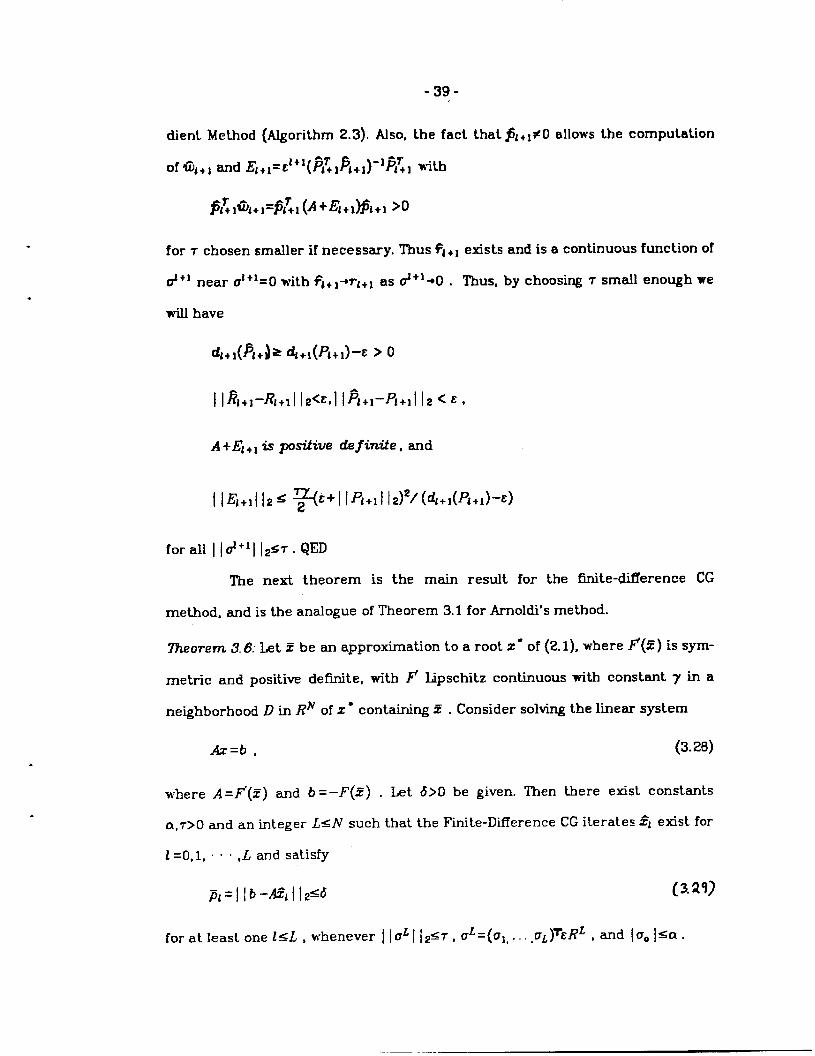
dient Method (Algorithm 2.3). Also, the fact that PI +1#0 allows the computation

~+’( PlzlP~+l)-%/ll withoftil+l and EJ+l=c

for 7 chosen smaller if necessary, Thus $1+1 exists and is a continuous function of

~+1 near u~+ko with F~+l+q+l as &+l+O . Thus, by choosing T small enough we.

will have

4+1(R+)= 4+1(PI+1)-C >0

I @l+l-R/+ll Ig<c,l @l+l-P~+ll Iz <z,

A +El +, is positive definite, and

I ll?j+~l 1*= ~z+l IR+l I 12)2/ (4+l(J3+J-&)

for all 11~+11 Iz<T. QED

The next theorem is the main result for the fhite-difference

method, and is the analogue of Theorem 3.1 for Arnoldl’s method.

CG

.

7heo~em 3. 6; Let Z be an approximation to a root Z* of (2.1), where F’(Z) is sym-

metric and posithw definite, with ~ I.ipschltz contiguous with constant 7 in a

neighborhood D in RN of z” contting ~ . Consider solving the linear system

Az=b , (3.28)

where A =F’(5) and b =–F(5) . Let 6>0 be given. Then there exist constants

cLT>O and an integer L4V such that the Finite-Difference CG iterates El exist for

1=0,1, “ “ “ ,L and satisfy

j5L=J]b-AfL 1124

for at least one l<L , whenever ] IaL I I2s7, d={ul . . . . ,UL)%RL , and

(3.29]

uOl=a.

(3.30)

“40-

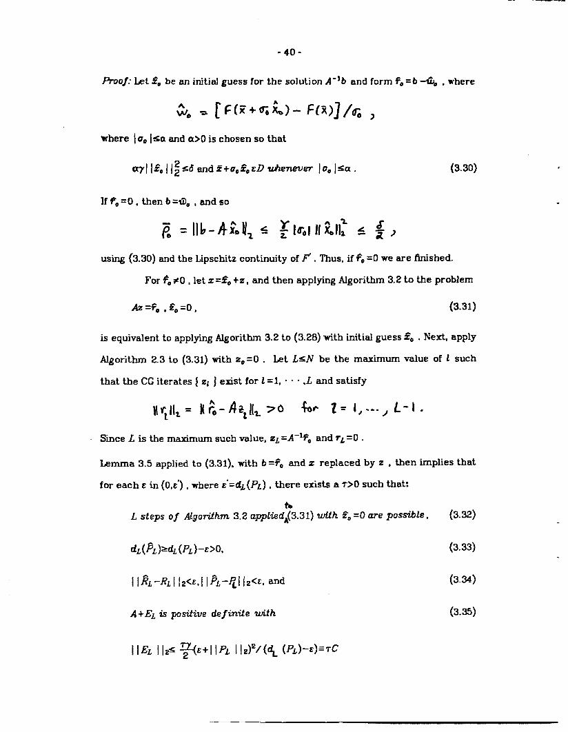
RooJ: Let 50 be an initial guess for the solution A-lb and form fO=b 40, where

$6 = r~( z+&)- f(x)~/G >

where ~UOI<a and a>O is chosen so that

a71!&ll~~d md~+aosoc~ tierz.ever ]Uo I<a,

If FO=O. then b=~o , and so

~ = llb-A&)lz + :Irolllilt s f )

using (3.30) and the Llpschltz continuity of F’ . Thus, if f. =0 we are finished.

For @o#O , let z =SO+Z, and then applying Algorithm 3.2 to the problem

AZ=FO, SO=O, (3.31)

is equivalent to applying Algorithm 3.2 to (3.28) with initial guess & . Next, apply

Algorithm 2.3 to (3.31) with Z.=0 . Let L=N be the maximum value of 1 such

that the CG iterates ~ Z1 j exist for 1=1, . . . ,L and satisfy

Iwtlll= l(wq(z >0 ~~ 1= L---, ~-l “

Since L is the maximum such value, z~ =A-leO and r~ =0 .

Lemma 3.5 applied to (3.31), with b =~o and z replaced by z , then implies that

for each &in (O,&”), where z’=dJ(P~) , there exists a T>O such thati

bL steps of Algonlhm 3.2 a~hkdA(3.31) tih 20=0 are possible, (3.32)

(3.33)

(3.34)

(3.35)

-41-

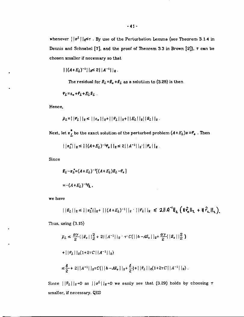
whenever [ I& I I~T . By use of the Perturbation Lemma (see Theorem 3.1.4 in

Dennis and Schnabel [7], and the proof of Theorem 3.3 in Brown [2]), T can be

chosen smaller if necessary so that

ll(A+~~)-’]l+211A-lllz.

The residual for EL=50 +EL as a solutiion to (3.28) is then

F’=co +f~ +ELs~ .

Hence,

PL=lln 112= ll&o112+ ll~L112+ llEL112Jl~Ll 12.

Next, let z: be the exact solution of the perturbed problem (A +EL)z =Fo .Then

lJz;112< ll(A+E~)-’Fo l[2<2JlA-ll 12”l/eot]2.

Since

i?A-z;=(A+E’)-l [(A+ E~)2L-PO]

=-(A+E’)-%L,

+llP~llz(l+27CllA-lllz)

<~+ 21~A-11 lzTC(llb–kAo112+$)+l l?~l]2(l+27CllA-11 12) .

Since ] ]FL ] 12+0 as I ld I 1240 we easily see that (3.29) holds by choosing T

smaller, if necessary. QED

. . . .__. ... . -. -_.&

-42-

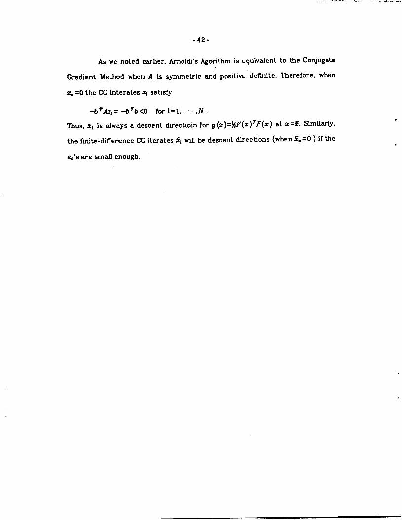
As we noted earlier, Arnoldi’s Agorithm is equivalent to the Conjugate

Gradient Method when A is symmetric and positive dellnite. Therefore, when

ZO=0 the CG interates Z1 satisfy

-b Y)kcj= -bTb<O forl=l, . “ . ,N .

Thus, 21 is always a descent direction for g (z)=)$F(z )TF(z) at z =Z. Similarly,

the fhite-dlf’ference CG iterates El will be descent directions (when &=0 ) if the

Ci’s are small enough.

.

●

.

.

-43-

4. Scaling and Preconditioning

The basic linear iteration methods considered in the previous sections are not of

much practical value as they stand. As dkcussed in [4], realistic problems

require the inclusion of scale factors, so that all vector norms become weighted

norms in the problem variables. However, even the scaled iterath’e methods

seem to be competitive only for a fairly narrow class of problems, characterized

mainly by tiiht clustering in the spectrum of the system Jacobian. Thus for

robustness, it is essential to enhance the methods further. As in other contexts

involving linear systems, preconditioning of the linear iteration is a natural

choice. In what follows, the use of scaling is reviewed, and then preconditioned

scaled iteration methods and algorithms are studied in a general setting.

(a) Scaling

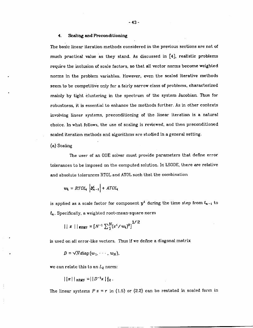
The user of an ODE solver must provide parameters that define error

tolerances to be imposed on the computed solution. In LSODE, there are relative

and absolute tolerances RTOL and ATOLsuch that the combination

w = RTO~ ~.l + ATO.&

is applied as a scale factor for component @ during the time step from in.1 to

&. Specifically, a weighted root-mean-square norm

is used on all error-like vectors. Thus if we define a dhagonal matrix

~ =~di.ug(wl, “ “ ‘ ,WN),

we can relate this to an .L2norm:

llzll~~~~=llD-’zj~~.

The linear systems P s = r in (1.5) or {2.2) can be restated in scaled form in

-44-

terms of D-i s = ~ and D-l r = -r. Likewise, the nonlinear system F(z) = O can .

be ,restated in a scaled form- ~(~)= O. The scaled version of the IOM algorithm,

denoted SIOM,is described in detail in [ 4 ].

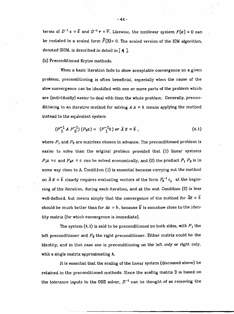
(b) Preconditioned Krylov methods.

When a basic iteration fails to show acceptable convergence on a given

problem, preconditioning is often beneficial, especially when the cause of the

S1OWconvergence can be identified with one or more parts of the problem which

are (individually) easier to deal with than the whole problem. Generally, precon-

ditioning in an iterative method for solving A z = b means applying the method

instead to the equivalent system

(4.1)

where P1 and P2 are matrices chosen in advance. The preconditioned problem is

easier to solve than the original problem provided that (1) linear systems

Plz =C and PSZ = c can be solved economically, and (2) the product PI P2 is in

some way close to A Condition (1) is essential because carrying out the method

onl~= 6 clearly requires evaluating vectors of the form Pk-) c, at the begin-

ning of the iteration, during each iteration, and at the end. Condition (2) is less

well-defied, but means simply that the convergence of the method for ~– = F

should be much better than for Az = b, because ~ is somehow close to the iden-

tity matrix (for which convergence is immediate).

The system (4. 1) is said to be preconditioned on both sides, with Pl the

left preconditioned and P2 the right precondltioner.

identity, and in that case one is precondkioning on

with a single matrix approximating A.

Either matrix could be the

the left only or right only,

]t is essential that the scalbg of the linear system (discussed above) be

retained in the preconditioned methods. Since the scaling matrix D is based on

the tolerance inputs to the ODE solver, D-* can be thought of as removing the

-45-

physical units from the components of z, so that the components of D-iz can be

considered dimensionless and mutually comparable. On the other hand, the

matrix A = I-h@O df / Oy is n~t similarly scaled, and so, because PI and P2 are

based on approximating A , the matrix

●

is also not similarly (dimensionally) scaled. More precisely, it is easy to show

that if the (i,j ) elements of PI and P2 each have the same physical dimension as

that of A , i.e. the dimension of ~i/~j, then so does the {i,~) element of ~ . The

same is true for the vectors 5 and ~: the ti_h component of each has the same

physical dimension as that of vi. It follows that the diagonal scaling D-] should

be applied to Z and ~ in the same way that it was applied to z and b without

preconditioning. Thus we change the system (4.1) again to the equivalent scaled

preconditioned system

.

.

Combining the two transformations, we have

An alternative point of view is to rescale the system first, to

(lI-’AD) (D-’z) = (D-%)

and then apply preconditioners QIJQ2 to D-l~, to get

(Q:lD-lADQ;l ) (Q2D-lZ) = (Q;lD-’b ) ,

(4.2)

(4.3)

But if the Q are unscaled to P~ = DQ D-l, this

system is identical to (4.2).

Consider now one of the Krylov subspace methods applied to the scaled

preconditioned problem. These methods all have in common the generation of

7,.

-,.’

-46-

t.he Krylov sequence

z+?.:l=o,l, ”””j -

from the initial residual ~0. We can assume that ~ = ~-&O corresponds to a

given initial guess ZO and residual ~ = b –AzO for the original problem, by way of

relatlons

F-a= D-1P2Z0 , FO = D-1P+. .

-The correction vector 2 -~0 is chosen from the span of the sequence K, trun-

cated to a given finite length (the number of linear iterations performed). But

from the relation ; = D-’P#, the subspace in which the correction z -zO is

chosen is instead the span of P>lDK (truncated), and this is the subspace we.

are ultimately interested in. Thus for a fixed matrix A and fixed initial residual

TO, define

This is the sequence whose fist 1 vectors are used to get zl -zO. The following

easy result helps to clarify the roles of left and right preconditioning.

Zhemem 4.1: The transformed Krylov sequence given by Eq. (4.4) satisfies

~(P~,P2) = K(l,P~ P~) = K(P~P~,f) . (4.5)

Roof: The general vector in the sequence K(P1,PZ) is

P~~D(D-IP;lfl~lD)tD”]P~*rO = P;’ (P~lAP~l )ZPj*rO .

= P~lP;l (AP~lPL#* = (P~lP;*A)lPSIPE1rC .

The last two expressions are identical to the corresponding vectors in ~(1,PIP2)

and K(PIPZ, 1) respectively. Notice that all D and D-l factors also drop out. QED

The above result says that the subspace of interest is independent of

the scahng matrix D, and independent of whether the two preconditioners PI

-47-

.

●

and P2 are applied on opposite sides or their product applied on one side or the

other. Moreover, if P] and Pz commute, the subspace is also unchanged if the

preconditioners are interchanged: K(Pl,~2)=K(P2, Pi). However, this indepen-

dence does n@ hold in the actual algorithms. Dependence on D is evident every

time a convergence test is applied to the norm of a vector. Dependence on the

arrangement of the preconditioners (as well as on D) arises in the posing of

orthogonality or minimality conditions on the residual. For example, in the

Arnoldi method the residual xi? – ?0 must be orthogonal to K1 (the 1-dimensional

subspace spanned by the first 1 vectors in ~), with ~e~l. This equivalently

rewritten as

D-lP;l (Az - To)LD-’P2KL with zeK1 = P/Dfl

in the case of preconditioners (Pi, P2). But for preconditloners (I, P1P2)thls con-

dition becomes

D-l(Az –r. )~D-1p1p2KL, ZCK1

and for preconditioners (P1P2,1) it becomes

D-lP;lP;l(Az -TO~D-lKj , Z~K~,

and the three conditions are not equivalent in general, although KLis the same

in all three.

(c) Preconditioned Krylov Algorithms.

For given preconditioners P, and P2, specific preconditioned algorithms result

from applying the basic IOM and GMRES algorithms of Sec. 2 to the transformed

%“system Az =b in (4.2). Most of the algorithmic issues that arise in the unprecon-

ditioned case carry over directly to the preconditioned case, and w’e will adopt

the same decisions that were made earlier (and described in [4]), as follows:

-40-

● We take ZO=0 , having no choice readily available that is clearly better.

● N-ewill incorporate the scaling in an explicit sense, storing

vectors ~i that arise in the method as it stands

“unscaled vectors fii =vi .

● We use a difference quotient representation

rather than

although in the code described in [4], we also included a user option to

supply Jv in closed form.

● We use the modified Gram-Schmidt procedure for orthogonalizing basis

vectors.

9 We handle breakdowns in the same same manner as in the basic algo-

rithms.

● We will use the same constant 6= .05 c1 as a bound on the residuals

IIb ‘kl ] ] WW.S(&l is the tolerance on the non- linear iteration).

The presence

algori t km, however.

operator

Av=z’-h@OJv,

of preconditioning does have some side effects on the

One is that we must actually deal with the

as opposed to dealhg with Jv and making corrections accordingly. This is

because the span [~ ,%-0, - 0c ,~[FO] is not generally the same as

[~ ,% ,...,~lfi ] With ~= D-lPFIJP~lD, unless PIPZ=I.

Secondly, the residual quantity g+ computed during the algorithm is

I l;~ I Iz = 11~-~! Ia and in general this is not directly related to the quantity

*

I ~~~! 1r..s = ] ! b -Az/ II IYRHSin which we are really interested. Instead, we have

a relation;, = D-*P;lr~ and hence

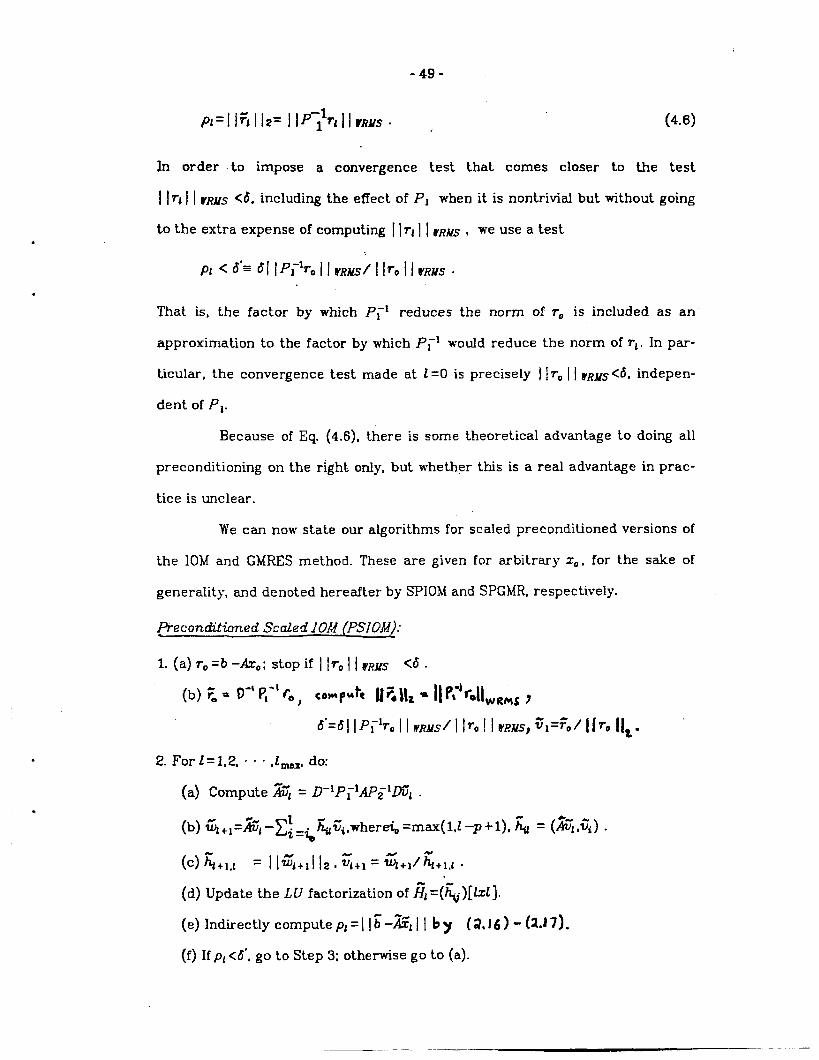
-49-

*

pi= (4.6)

In order to impose a convergence test that comes closer to the test

I Irl I I VRMS<b. including the effect of PI when it is nontrivial but without going

.

That is, the factor by which P;* reduces the norm of r. is included as an

approximation to the factor by which Pil would reduce the norm of rl. In par-

ticular, the convergence test made at 1=0 is precisely IITO\I gRJfS<d, indepen-

dent of P,.

Because of Eq. (4.6), there is some theoretical advantage to doing all

preconditioning on the right only, but whether this is a real advantage in prac-

tice is unclear.

We can now state our algorithms for scaled preconditioned versions of

the IOM and GMRES method. These are given for arbitrary Z,, for the sake of

generality, and denoted hereafter by SPIOhi and SPGMR, respectively.

.

.

2. Forl=l,2, , .. ,1-, do:

(a) Compute ~~ = D-lPrlAP~lfi-l .

(b) ~+l=kl-~~=~fi~i,where~o =max(l,l -P+l), L = (~~,fii) .

(c) ~+l., = I Itil+ll 1~, q+, = q+,/ fi+*.i .

(d) Update the LU factorization of fil =~~)[lzl].

(e) Indirectly compute pi=11 ~-~1 \ I by (2, 16) - (XJ7).

(f) Ifpl<d”. go to Step 3; otherwise go to (a).

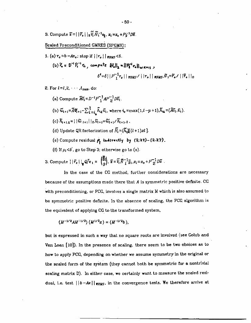
Scaled Preconditioned GMRES(SPGMR):

1. (a) TO=b -AzO; stop if I ITOI ] ~R#~Cd.

2. Forl=l.2, . “ “

(a) Compute

(b) fi~+l=~~+l-~}=io&&, where& =max(l,l -p +l),zt=(~fil.~~).

(c) &+,,t=} la ~+,1l@J+l=a~+l/z+l,l .

(d) Update QR factorization of ~l=(~j[(l +l)z1 ].

(e) Compute residual ~1 hd{rcctty by (%aV)- {2.27).

(f) If p, <6”, go to Step 3; otherwise go to (a).

In the case of the CG method, further considerations are necessary

because of the assumptions made there that A is symmetric positive definite. CG

&ith preconditioning, or PCG, involves a single matrix M which is also assumed to

be symmetric positive definite. In the absence of scaling, the PCG.algorithm is

the equivalent of applying CG to the transformed system,

but is expressed in such a way that no square roots are involved (see Golub and

VarI Loan [10]). In the presence of scaling, there seem to be two choices as to

how to appIy PCG, depending on whether we assume symmetry in the original or!.

the scaled form of the system (they cannot both be symmetric for a nontrivial

scaling matrix D). In either case, we certainly want to measure the scaled resi-

dua~ i.e. test I Ib –Az I~~RN~,in the convergence tests. We therefore arrive at

.

.

●

✎

-51-

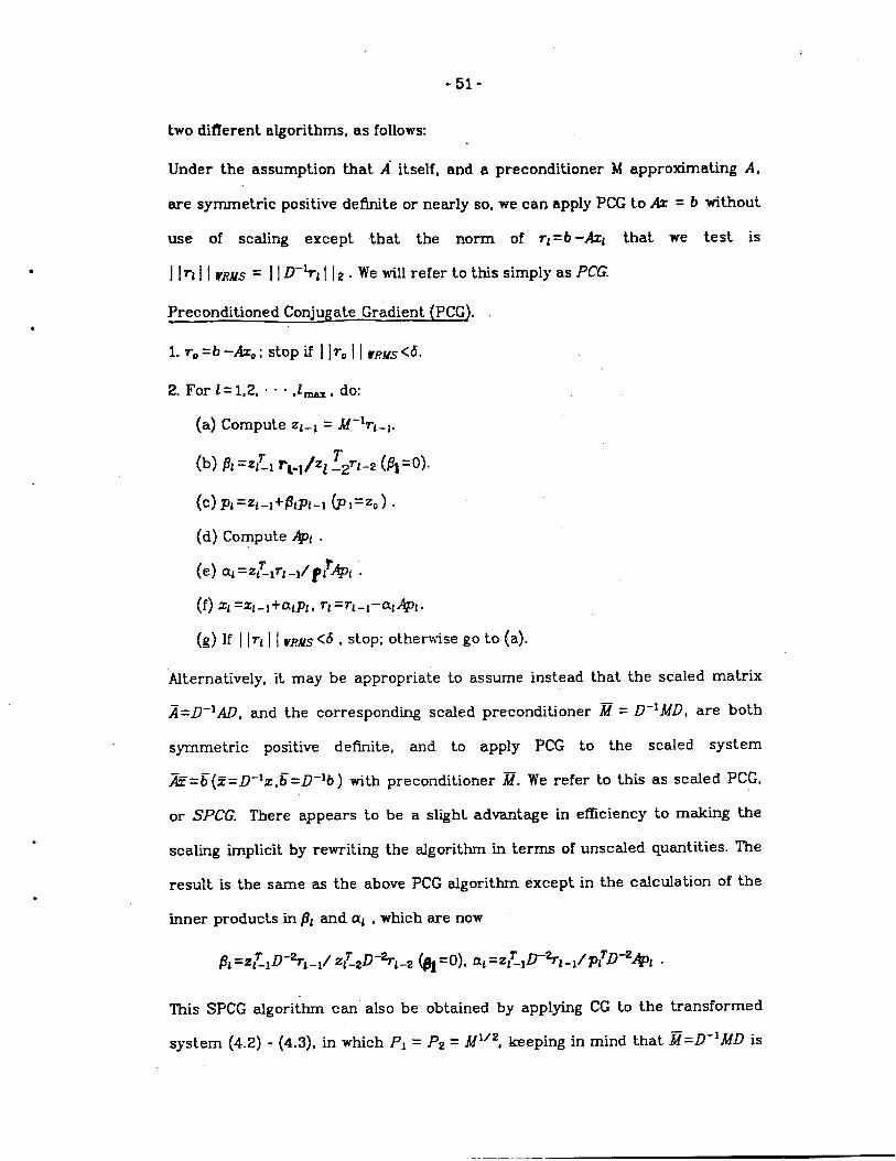
two different algorithms, as follows:

Under the assumption that A- itself, and a precondltioner M approximating A,

are symmetric positive definite or nearly so, we can apply PCG to AZ = b without

use of scaling except that the norm of rl =b –Azf that we test is

j Irl I ~~RMS= 1]D-%l I ~~ . We will refer to this simply as PCG.

Preconditioned Conjugate Gradient (PCG).

1. rO=b-AzO; stop if ] ITOI ] ~~~s<d.

Alternatively, it may be appropriate to assume instead that the scaled matrix

~=D-lAD, and the corresponding scaled precondltioner ~ = D-~MD, are both

symmetric positive delhite, and to apply PCG to the scaled system

k-= F(Z=D-lz,~=D-lb) with

or SPCG. There appears to

scaling implicit by rewriting

precondltioner ~. We refer to this as scaled PCG,

be a slight advantage in efficiency to making the

the algorithm in terms of unscaled quantities. The

result “Mthe same as the above PCG algorithm except in the calculation of the

inner products in @l and al , which are now

~1=z~lD-&/ z/’_zD-%j_z @ =0), & =z~-lD-%i_#p~D-2& .

This SPCG algorithm can also be obtained by applying CG to the transformed

system (4.2) - (4.3), in which PI = P2 = M1lZ, keeping in mind that ~= D-lMD is

K.. ..+— -.

-52-

assumed to be symmetric, whfle M and Ml’z = D~l’2D-1 are not (in general).

We have implemented both PCG and SPCG, filling in algorithm details in

the same way as done for the other methods (using ZO = O, a difference quotient

&,6=.05 cl, etc.). Of course, ‘each algorithm is subject to breakdown when applied

to a problem for which the assumed symmetry or definiteness fails to hold. Thus

the denominators in @l and al are tested for being zero before the dNide is

done.

.

.

-——.

-53-

.

.

5. Preconditioners for Reaction-Diffusion Systems

The preconditioned Krylov subspace methods described so far are quite general

in nature, with preconditioned matrices that are as yet unspecified. In this sec-

tion some specific choices will be described, as motivated by ODEsystems that

arise from PDE systems by” the method of lines (MOL). At this point, our

approach attempts to compromise between totally general methods, in which

problem structure is not exploited at all, and totally ad hnc solution schemes, in

which the algorithm and problem features are so closely linked that flexibility as

to problem scope is lost. Here the preconditioners will exploit problem struc-

ture, wit,hln a setting of general purpose methods (BDF, Newton, and Krylov). The

general and special parts of the algorithm are logically well separated. To the

extent that some storage for precondltioner matrices (and associated data) will

be required, our methods are no longer truly matrix-free in some cases. How-

ever, since storage economy (as compared to traditional stiff system methods)

is still a prime concern, any choice of preconditioners should be strongly

influenced by its storage costs.

(a) Problem Structure.

The class of problems we shall concentrate on here is that of ODE sys-

tems in time that are the result of treating time-dependent PDE systems by

some form of the method of lines. Assume that a vector u =U (t ,x ) of length p is

governed by a PDE system in time f and a space variable z (of any dimension) of

the form

au/at= R(t,z,u) + S(t,z,u), (5.1)

plus initial and boundary conditions, in which R represents reaction terms and S

represents a spatlai transport operator in z (diffusion, advection, etc.). Thus R

is assumed to be a point function of u , while S cent ains partial derivatives of u

with respect to z. The MOLtreatment of such a system consists of representing

the spatial

discretized

-54-

variatlon of u in a discrete manner, and thereby obtaining a semi-.

form of (5.1) in which S is replaced by a dkcrete function, while the

time derivative remains continuous. TO be more specific, but without dWressing

unduly into MOLtechniques, consider tratitiona fite difference discretizations

of (5. 1). In this case, discrete values Ui represent

points ~ and suitable difference approximations to

the boundary conditions are formed. The vector

Y=(%*‘ “ “J

of length IV=pg then satisfies an ODE system

J=R(t~,y) + S(t,y),

with given initial conditions, in which ~ and ~

Of course there are many variations

u(f ,~) at g discrete mesh

S(t,z,u) at each ~, and to

(5.2)

are discrete forms of R and S.

on this approach (staggered grids,

moving grids, etc. ) and there are radically different discretization choices, not-

ably the various finite element schemes. The latter generally result in OD~;sys-

tems that are linearly implicit, with a square mass matrix multiplying y. For the

present, we will assume that, n7hatever the spatial discretization, the ODE sys-

tem has been put into the explicit form (5.2) (possibly by multiplying by the

inverse of a mass matrix), although it is a straightfomsard matter to extend our

methods so as to treat linearly implicit systems as such. In order to reflect this

greater generality in (5.2), we will denote the global vector y as

l/=(Yll “ “ “ ,Yq)T (5.3)

in which each of the g blocks Vi (each of length p) is associated with a point

z=%, but may or may not represent a discrete value of the original vector u in

(5.1).

In (5.2), the essential feature of the additive splitting ~+~ is that ~ does not

-55-

.

.

.

.

involve any spatial coupling, while ~ invglves little or no interaction between the

components of Vi at any given point Zi. Thus the individual blocks of (5.2) can be

written

?ii=fi(f s?/)= R(f,Yi) + ~i(t~’!/l~ “ “ “ oYq)* (5.4)

where R is a function of vi but no other ~j, while the dominmt feature of ~i is

the coupliig among various vi arising from the dhscretization of spatial deriva-

thes.

(b) Block-Diagonal reconditioners.

To obtain a preconditioned matrix M that is intended to approximate

the Newton matrix A=I–h& J, the most obvious approach is to consider a

matrix L that approximates the system Jacobian J, and use M=I-h& L. For the

blocked ODE system given by (5.2)-(5.4), a natural choice for L is one that is

block-dkgonal and hence can accurately reflect the interaction of the com-

ponents at each spatial point, but not the spatial coupling. Thus consider a

block-diagonal matrix

B=d*(131, “ “ “ ,Bq)

in which each Bi is pzp. We can get B to approximate J in one of two ways:

(5.5)

Bi =Of i/ d~i (i*h d~goti block of J)

or

& ‘~Fi/ dyi .

We will refer to these choices as the total block-diagonal

(5.6)

(5.7)

and the interaction-

o~ approximations, respectively. ‘hey differ by ~~i / Oyi , the diagonal Put Of

the dkcrete transport Jacobian.

In either case, the computation and processing of the matrix B and M=l –h~o B

is certainly a nontrivial matter. It may be that the problem permits the Bi to be

..-

~

. . ...

-56-

supplied “m closed form fairly cheaply, but in most practical cases, we expect

that this is not feasible. Then a difference quotient approximation to Bi must be

done. For this, we assume that a routine to compute the individual blocks

~i(f W) (in the total case) or ~i (t ,yt) (in the interaction only case) is supplied

and is reasonably inexpensive. The cost of one such evaluation would be

expected to be about 1/g Klmes that of evaluating all of ~ (t ,y ) =& (somewhat

more in the total case, somewhat less in the interaction only case). Then a

difference quotient estimate of Bi will involve p such calls (assuming a base

value of ~i or ~i is saved for use ~ the difference quotients, but ~fithout exploit-

ing any sparsity structure within Bi), and the total cost of B wi. be about that of

fJ evaluations of ~.

Once 1? is evaluated, it is subjected to LU decomposition, and the LU

factors of the blocks are saved. Then these are used as needed whenever a vec-

tor B-% is called for. Periodic reevaluation of B is done by the same strategy

used for traditional methods involving evaluation and use of the Jacobian J.

Tbe block-diagonal structure of B allows for considerable potential

speedup if the scheme is implemented on a multiprocesso~. The various blocks,

corresponding to the various spatial points, can be evaluated, then factored, and

the factors applied to a given (blocked) vector, all in parallel with one another.

As many as g processors can be occupied concurrently for a problem with g

mesh points. Block-diagonal preconditioning can be expected to improve per-

formance considerably when the interaction among the components of u at

each point z is the dominant contributor to the stiffness of the system (5.2). The

inclusion of part of the transport contilbution, as done in (5.6), may or may not

improve performance further.

The storage cost is clearly an additional pzq = pN words, to hold the

.

~i and then their factors. Tlis cost could well be greater than that of all of the

-57-

.

.

remaining work space involved when p is sizable, although not nearly as big as

the cost of storing all of the Jacobian and its LU factorization in a typical multi-

dimensional system treated by a traditional method.

A natural way to reduce the storage cost is to do grouping of the diago-

nal blocks Ba. By this we mean that the spatial points are grouped, most likely

by a simple decomposition of the original spatial domain, and for each group

only one l?a is evaluated and used as an approximation to the others in the

group. This is simply the analog in space of the strategy of periodic Jacobian

evaluations in time - a strategy which is widely used and hWhly cost- effective. In

both ideas, the motivation is that the Jacobian elements needed are likely to

vary smoothly as functions of the relevant independent variable (space or time)

and so need only be evaluated on some subset of the discrete values of that vari-

able that are generated. The resulting crude approximation to Jacobian ele-

ments is acceptable within a New-ton iteration, whereas the full set of discrete

values is dictated by the accuracy of the final computed solution. lf the q spa-

tial points Za are somehow grouped into g groups (not necessarily of equal size)

then the cost of evaluating the grouped block- diagonal approximation B goes

down to about p (g / q ) evaluations of j, and the storage is reduced to pzg. Thus

there is a potentially great reduction in storage costs with grouping, but the

reduction in computing cost depends on whether significantly more linear

and/or nonlinear iterations must be taken than were taken without grouping.

(c) Transport-8ased ~reconditioners.

Another natural choice presents itself for blocked problems of the type

(5.2)- (5.4), namely a preconditioned that uses the discretized transport opera-

tor ~i. Here the interaction of the components at each point is ignored, and for

each component separately, a precondltiloner arises upon treating the transport

contributions of the problem by traditional iterative methods such as SOR (suc-

...

-58-

cessive overrelaxation). The details of this preconditioned will depend heavily on

the particular nature of the- problem. In order to be somewhat specific here,

suppose that the transport occurs linearly in ~i , so that we can write

Assume further that the various coefficient blocks

(5.8)

(all pq) in (5.8) are diagonal,

reflecting the fact that component interaction is completely accounted for in the

term R~ Of (5.4).

Then the blocked matrix

(5.9)

is an approximation to d~/ dy on which a preconditioned can be based. (It may

not be all of ~~/@ because the coefficients might depend on y, and that

dependence is being ignored here. ) The corresponding approximation to

A=I–~T is

which

B-L– V=(I-h$O~) - h~o~–hflo ~,

also has diagonal pzp blocks.

Now consider, for example, the application of SORto the system

(B-L-U)Z =b. , (5.10)

We must suppose that the acceleration parameter u is given, and if no better

information about its choice is available, we may simply have O= 1 {and we are

doing Gauss-Seidel iteration). The tiltial guess is some easily computable vector

Z’J = &b, where the matrix JIO might be O, or B-l. or 0(f3-uL)-1, for example.

(1 n O* +%+s , w .,, fi third~bi.cfm M.t’)

.

.

.

.

.

The iteration is given by

2“+’42” +L)(B-CJL)-%

with

z = (B-UL)-l [(l-U)B+WU]C

Thus a given number, m,

Zm= m +( F+

where

-59-

of iterations produces an iterate

&4+ ●*. +~+I)u(B-@-lb =Mb ,

(5.11)

This matrix 14 represents a preconditioned for the system AZ = b. In practice, it

would be applied by carrying out the S(IR iteration in whatever manner is most

appropriate for the particular problem, depending on the number of spatial

dimensions, the boundary conditions, the uniformity or variation of the

coefficients, etc. Keeping storage to a minimum would be an important criterion

in the implementation.

An easy variation of SOR as a preconditioned is Symmetric SOR, or SSOR, where

each iteration has a forward and a backward sweep:

z“+’” =<2” + (B-tiL)-’ub

where~= (ll-uU)-l[(l-u) B+uL].

Some given number of SSOR iterations, say m, has the same cost as 27n SOR

iterations, but may be more effective because of the symmetrizatkm.

In special cases, one might be able to do even better in approximating

the solution of (5. 10). For example, suppose that the dominant transport pro-

cess is simple diffusion, that the mesh is uniform, and that for each PIIE

-f30-

component the diflusion coefficient is constant. Then the product Jz represents

a decoupled set of discrete diffusion operators (with source term), dV% +r and

the system AZ= z -h&Jz =b, after dhision by h/30d in each PDE component,

corresponds to a collection of scalar Helmholtz equations

Au+v%l = s’ , A=-l/h@. tf ,

discretized on a uniform mesh. For such a probIem, fast Poisson solvers are

available. To the extent that the diffusion operator dominates the physical tran-

sport process, the resulting preconditoner should be very effective.

It should be emphasized that in all of the above cases, the various PDE

components, i.e. the components of the vector u ih (5. 1), are treated indepen-

dently. Whichever of these preconditioners is used, it’ is apphed separately to

each PDE component. in particular, the implementation of the combined

algorighm on a multiprocessor could readily take advantage of this fact by car-

rying out the preconditioning operations concurrently for the various com-

ponents.

(d) Operator Splitting.

The preceding

without saying just how

paragraphs give specific preconditioned matrices

they are to be applied. Clearly, if a single matrix is

chosen as a preconditioned, it can be applied on the left as P, or on the right as

Pz in the SPIOMor SPGMR algorithms, or as the matrix M in PCG or SPCG. But if

two dMferent matrices are available as preconditioners, then in SPIOM or SPGMR

they can be applied as Pl, and P2, in either order, or their Product (in either

order) could be applied on one side only, or the product applied as M in PCG or

SPCG. There seems to be no convincing argument for or aga-mst any particular

choice of arrangements of the precondltloners for a given Krylov algorithm.

For the reaction-transport problems described above, choosing both a block-

diagonal (presumably the interaction-only choice) and a transport-based

-61-

.

.

preconditioned constitutes an operator splitting approach to preconditioning

that closely resembles split&g methods used elsewhere. The block-diagonal

matrix 13 is dominated by the interaction of tie PDE components at each spatial

point, while the transport-based matrix M attempts to account for the

remainder of the problem. Each matrix can be dealt with reasonably efficiently,

in contrast to the matrix J=a$ / ~y which reflects both the interaction and the

transport operators.

This splitting approach obviously generahzes in “the same sense that

traditional splitting methods do, to ODE systems with any additive spIitting. Thus

suppose the system is

j =f = f,+f2+”””+A ,

with the various terms ~k representing distinct physic~ processes (operators).

Assume further that the indhidual Jacobian matrices ~k ‘hfk /&/ are easilY

computed or approximated in such a way that a sYstem(~-h& ‘k )z’~ can be

solved (or approximately solved) efficiently. Then each matrix Au=J-h~OJk (or

a computable approximation to it) serves as a preconditioned and the product of

Al, .” ,4, is a single preconditioned to the linear system Az =b ,A=I -APOJ .

Two products, of two subsets of these Ah co~d be used as left and right Precon-

ditioners. The best choice of order in the products is unclear in general, and

performance may not depend strongly on the order. Heuristically, the use of

P=A1A2 . ● . 4 as a preconditioned would be expected to do well to the extent

that P approximates A, i.e. to the extent that

The two matilces above agree only to first “order in h The errors in P associated

with higher order terms would have to be dealt with by the Krylov method in

order for the combination to be effective.

-42-

6. Numerical Tests

Tests of the methods described above were done using an experimental

solver derived fom the general purpose ODE solver LSODE,which uses BDF

methods for stiff problems. Stiff test problems were generated by applying

the method of lines to PDE systems in two space dimensions. What follows is

a brief description of the solver, and a description of tests on three prob-

lems. All testing ‘was done on a Cray-1 at LLNL.

(a) BODPK, an Experimental Solver.

A solver package called LSODPK @ivermore Solver for ODES with Precondi-

tionned Krylov methods) was created from LSODE, in which to implement the

preconditioned iteration methods. LSODPK resembles the solver LSODP

described in [4], which uses (unpreconditioned) Arnoldl and IOM. LSODPKallows

the user to select among Arnoldi/IOM, GMRES, PCG, and SPCG as the basic itera-

tion method, and accepts user-supplied routines to accomplish the precondi-

tioning operations. Thk is shown in a simplified form in Fig. 1. The driver rou-

tine, LSODP~ calls a single-step routine, STODP~ which calls PKSET to prepare

for preconditioning, and SOLPKto carry out the linear system solution by calling

one of four other routilnes, as shown. The user supplies F (for f ( t .y ) as in

LSODE, but also two routines, JAC and J%O~ for preconditioning. (All three

names are dummy names, passed by the user to LSODPK.) JAC must oufuh *“wIpre-

process any Jacobi an-related data involved i n the preconditioning.

PSOL mu$t carry out the preconditioning of a vector, i .e. replace a

vector v vi th P~lv, P&v, or ?~%, depending on the choice of method

and the nature of the preconditioning. Various integer flags are input

by the user to specify these choices, and a flag is passed to PSOL to

spec~ fy which FklV is desired when both are possible.

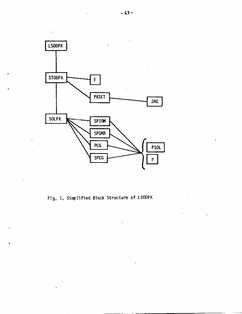
-43-

●

☛

TLSODPK

v

STODPK

JAC

I

SOLPK

Fig. 1. Simplified Block Structure of LSODPK

.

.

,: .. . ~...=:.’..+ -.

-64- -“y.,.-:,<...,*...

in all other respects, the overall algorithm in LSODPK is the same as LSODE

and/or LSODP. Calls to PKSET (hence to JAC) are made as infrequently as judged

suitable, by the same heuristic rules that govern J evaluation in LSODE. As in

LSODP, the default value of the heuristic convergence test constant 6~ . is .05 (:.@. s=. brc, &

that of lm~ is 5, and that of the parameter p

incomplete methods).

Various cumulative performance

LSODPK. These include:

NST = number of time steps

is lXU (giving complete rather than .

.statistics are made available by

NFE = number of j eva~uations

NPE = number of preconditioned evaluations (JAC calls)

NNI = number of nonlhear iterations

NLJ= number of linear iterations

NPS = number of preconditioned solves (PSOL calls)

NCFN= number of nonlinear convergence failures

NCFL = number of linear convergence failures

NF’Eis also equal to NW + NLI + 1 (plus the number of internal restarts at order

1, if any). In addNion, LSODPKmonitors the average Krylov subspace dimension

Avmh4 = A ml /ANNl,,

and the convergence failure rates

RCFN = A NCFN/ A NST

R(2?L = A NCFL/ 4 NNl

W’ithln an output interval. Warning messages are printed if these appear to be

too large.

Wkdle the preconditioning routines JAC and PSOL are not part of the

LSODPK solver as such, we have generated several pairs of routines for use on

tests in PDE-based problems. One such pair generates the total block-diagonal

●

●

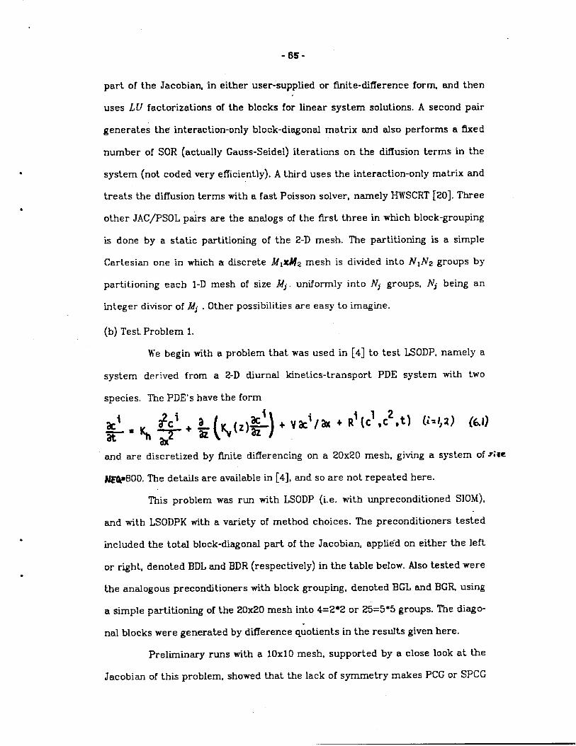
-65-

part of the Jacobian in either user-supplied or finite-difference form and then

uses L U fact orizations of the blocks for linear system solutions. A second pair

generates the interaction-only block-diagonal matrix and also performs a fixed

number of SOR (actually Gauss-Seidel) iterations on the dillusion terms in the

system (not coded very efficiently). A third uses the interaction-only matrix and

treats the dh7usion terms with a fast Poisson solver, namely HWSCRT[20]. Three

other JAC/PSOL pairs are the analogs of the first three in which block-grouping

is done by a static partitioning of the 2-D mesh.

Cartesian one in which a dkcrete ~l%~z mesh is

partitioning each 1-D mesh of size Mj. uniformly

The partitioning is a simple

divided into NIN2 groups by

into Nj groups, Nj being an

‘integer divisor of Mj . Other possibilities are easy to imagine.

(b) Test. Problem 1.

We begin with a problem that was used in [4] to test LSOI)P, namely a

system derived from a 2-D diurnal kinetics-transport

species. The PDE’s have the form

PDE system with tw’o

,c*,t) U=1)2) (61)

and are discretized by finite differencing on a 20x20 mesh, giving a system of ~~ze

NE@100. The details are available in [4], and so are not repeated here.

This problem was run with LSODP (i.e. with unpreconditioned SIOM),

and with LSODPK with a variety of method choices. The precondltioners tested

included the total block-diagonal part of the Jacobian, applie-d on either the left

or right, denoted BDL and BDR (respectively) in the table below. Also tested were

the analogous preconditioners with block grouping, denoted BGL and BGFLusing

a simple partitioning of the 20x20 mesh into 4=2*2 or 25=5*5 groups. The diago-

nal blocks were generated by difference quotients in the results given here.

Prelii-mary runs with a 10x1O mesh, supported by a close look at the

Jacobian of this problem, showed that the lack of symmetry makes PCG or SPCG

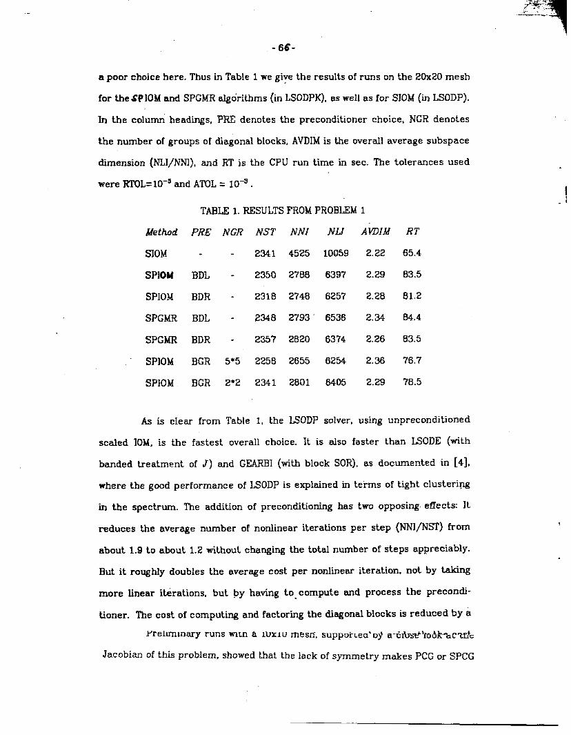
‘T;;+&l-

,<,.. .. -----%.----s. ..

-66-

a poor choice here. Thus in Table 1 we give the results of runs on the 20x20 mesh

for the @IOM and SPGMR algorithms (in LSODPK), as well as for SIOM (in LSODP).

In the column headings, PRE denotes the precond~tioner choice, NGR denotes

the number of groups of diagonal blocks, AVDIMis the overall average subspace

dimension (NL1/NNl), and RT is the CPU run time in sec. The tolerances used

were RTOL=10-s and ATOL= 10-9.

TABLE 1. RESULTSFROMPRQBLEM1

MetAad PRE

SIOM -

SPIOM BDL

SPIOM BDR

SPGMR BDL

SPGMR BDR

- SPIOM BGR

SPIOM BGR

NGR

.

5*5

2*2

NST NNI

2341 4525

2350 2788

2318 2’?48

2348 2793

2357 2820

2258 2655

2341 2801

NLJ

10059

6397

6257

6536

6374

6254

6405

AhIM RT

2.22 65.4

2.29 83.5

2.28 81.2

2.34 84.4

2.26 83.5

2.36 76.7

2.29 78.5

As is clear from Table 1, the LSODP solver, using unpreconditioned

scaled IOM, is the fastest overall choice. It is also faster than LSODE (with

banded treatment of J) and GEARB1(with block SOR), as documented in [4],

where the good performance of LSODP is explained in terms of Vlght clustering

in the spectrum. The addition of preconditioning has two opposing. effects: It

reduces the average number of nonlinear iterations per step (NN1/NST) from

about 1.9 to about 1.2 without changing the total number of steps appreciably.

But it roughly doubles the average cost per nonlinear iteration, not by taking

more linear iterations, but by having to compute and process the precondi-

tioned. The cost of computing and factoring the diagonal blocks is reduced by a

rremmnary runs Ntn ~ l~xl u rnesn-, suppoixea’ D~ a-rhbst?’fbtk-a~lf).

Jacobian of this problem, showed that the lack of symmetry makes PCG or SPCG

.

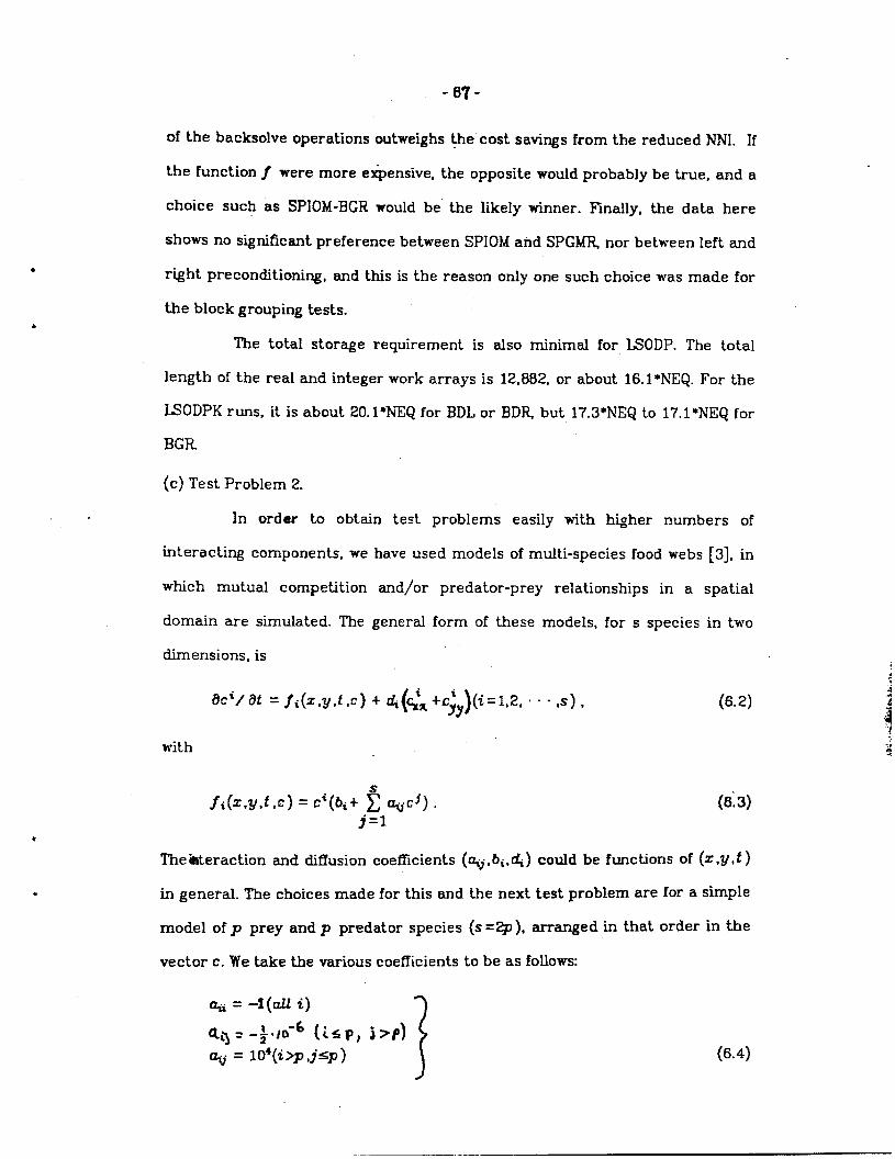
-07-

of the backsolve operations outweighs the’ cost savings from the reduced NNI. If

the function j were more e@ensive, the opposite would probably be true, and a

choice such as SPIOM-BGR would be the likeIy winner. Finally, the data here

shows no significant preference between SP]OM and SPGM~ nor between left and

right preconditioning, and this is the reason only one such choice was made for

the block grouping tests.

The total storage requirement is also minimal for

length of the real and integer work arrays is 12,882, or about

LSODP. The total

16.1 *NEQ. For the

LSODPK runs, it is about

BGR

(c) Test Problem 2.

20. l*NEQ for BDL or BD~ but 17.3*NEQ to 17.1 *NEQ for

In order to obtain test problems easily with Klgher numbers of

interacting components, we have used models of multi-species food webs [3], in

which mutual competition and/or predator-prey rela~lonships in a spatial

domain are simulated. The general form of these models, for s species in two

dimensions, is

ac~/ at = ~i(z,vt~,c) + 4(<~+CjY)(~=l,2, “ “ “ ,S) , (6.2)

with

fi(z.~,~,c) = Ci(bi+ J ~cj) . (63)j=l

The interaction and diffusion coefficients (~ ,bi.~ ) could be functions of (z .Yi t )

in general. The choices made for this and the next test problem are for a simple

model of p prey and p predator species (s =2p ), arranged

vector c. We take the various coefficients to be as follows:

in that order in the

(6.4)

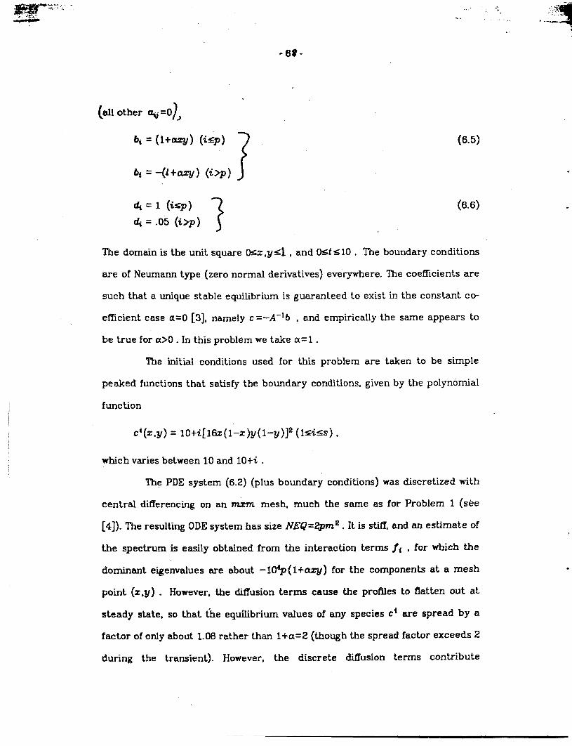
#ggp-””-

“68-

.!.

“...s. . . .,..-:

-, ., ..-

.

( )all other aij =0 ~

4 = 1 (i<p)

1

(6.6)

rf, = .05 (i>p)

The domain is the unit square 04z ,y<l , and Et= 10. ‘f’he boundary conditions

are of Neumam type (zero normal derivatives) everywhere. The coefficients are

such that a unique stable equilibrium is guaranteed to exist in the constant co-

efficient case 0!=0 [3], namely c =-A-lb , and empirically the same appears to

be true for a>O . In this problem we take a= 1.

The initial conditions used for this problem are taken to be simple

peaked functions that satisfy the boundary conditions, given by the polynomial

function

Ci(z,y) = lo+i[16z(l-z)y( l-y)]2 (l<i<s) ,

which varies between 10 and 10+~ .

The PDE system (6.2) (plus boundary conditions) was discretized with

central dlfferencing on an nmm mesh, much the same as for Problem 1 (see

[4]). The resulting ODEsystem has size NEQ=2pwa2. R is stiff, and an estimate of

the spectrum is easily obtained from the interaction terms ii , for which tie

dominant eigenvalues are about -l&P( l+asy) for the components at a mesh

point (z,Y) . However, the diffusion terms cause the profiles to flatten out at

steady state, so that the equilibrium values of any species Ct are spread by a

factor of only about 1.06 rather than l+a=2 (though the spread factor exceeds 2

.

.

during the transient). However, the discrete diffusion terms contribute

. . ..

significantly to the stiffness also,

*

●

For the tests reported here, we take m =12 (144 mesh points), and we

take two cases for p ,

(a) P=5 (10 species, NEQ= 1440),

(b) p= 10 (20 species, NEQ = 2880).

we report results for LSODPK with a variety of method choices. The tolerances

used were RTOL = 10-6 and ATOL = lo-e . The pCG and SPCG methods were not

tested because the Jacobian at equilibrium is highly nonsyrnmetric. The precon-

ditioned pairs tested, with mnemonic names used in the tables, are as follows:

BDL total block-diagonal part of J on lefti

BDR total block-diagonal part of J on right;

0SS: operator splitting, using 5 SOR (Gauss-Seidel) iterations on the

diffusion terms for PI and the interaction-only Jacobian for P2;

(XY? operator splitting, using HWSCRTon the diffusion for PI and the

interaction-only Jacobian for P2 .

Where a block-diagonal part of the Jacobian J is required, both a closed-form

user-supplied option (USJ) and a difference quotient option from (DQJ) were

tested. Further, we tested the analogous set of preconditioned pairs in which

block group-mg was done, with NGR =% ~ groups from a Cartesian product par-

tition of the mesh with ~ groups in each dimension ( ~ a dhision of 12). All the

various possible combinations are too numerous to test completely. Nor did we

test the other possible arrangements of the precondltioners (interchanging P1

with P2 . or using the product on one side only), as we do not expect those to

yield major variations in performance. However, we did run tests using the indi-

vidual precondltioners in 0SS by themselves, i.e.

,. ..’ .,..

—

-70-

SOR left preconditioning with 5 SOR (actually Gauss-Seidel) iterations;

10J right preconditioning with interaction-only Jacobian.

Table 2a gives results for the 10-species case (p =5) , beginning with

those from SIOM (without preconditioning). We see that various precondi-

tioned method combinations do better than SIOM, both in statistics and run

time. The benefits of preconditioning in reducing the number of linear and

nonlinear iterations per step, and also the number of failed steps and step

size reductions forced by convergence failures, is clear for the SPGMR

method with 0SS and OSF precondltiloning. The BDL and BDR choices give

competitive run times but with much higher average numbers of (the aper)

linear iterations per step- a tradeoff of dubious merit when more costly

forms f are contemplated. The one-sided choices SOR and IOJ fail even

more badly. The OSF choice is more expensive than 0SS here because the 5

SOR iterations are evidently cheaper than the HWSCRT call and nearly as

effective. For the same problem with more di.fhion, namely ~= 10 (2<5) ,

the preference order is reversed, with run times of 54 for OSS (where 10~w

SOR iterations was found necessary) vs 38~OSF. From the close agreement

between SPGMR and SPIOMperformance, with either 0SS or BDR precondi-

tioning, no further testing of SPIOM seemed to be worth doing. The use of

block grouping with 0SS raised AVDIMonly slightly, but reduced the co’st

slightly and reduced the required storage considerably - by a factor of

.

.

- ““”’--.,.”.-

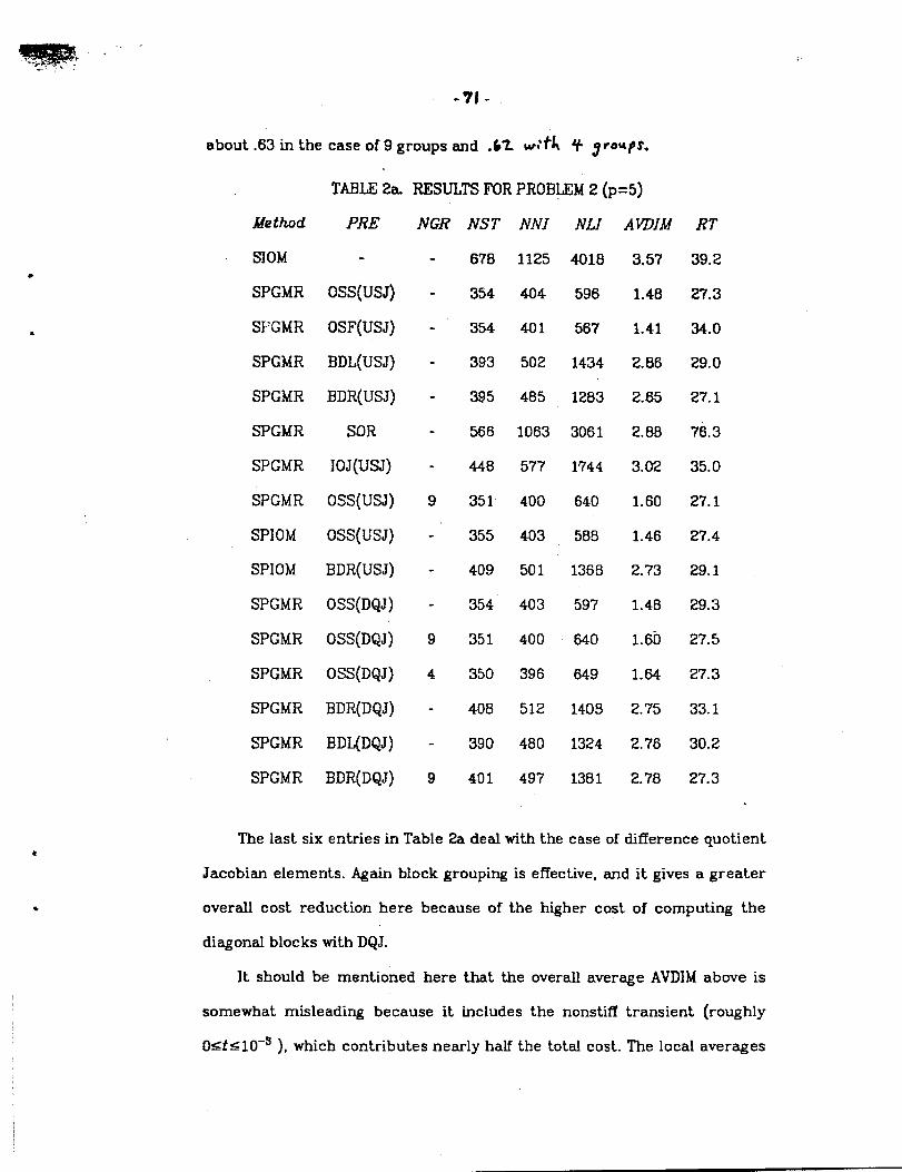
-.-71-

about .63 in the case of 9 groups and .62 w:t~ 4 g re~pS.

TABLE2a. RESULTSFOR PROBLEM2 (p=5)

MetAod

SIOM

SPGMR

SI’GMR

SPGMR

SPGMR

SPGMR

SPGMR

SPGMR

SPIOM

SPIOM

SPGMR

SPGMR

SPGMR

SPGMR

SPGMR

SPGMR

PRE

OSS(USJ)

OSF(USJ)

BDL(USJ)

BDR(USJ)

SOR

IOJ(USJ)

OSS(USJ)

OSS(USJ)

BDR(USJ)

OSS{DQJ)

OSS(DQJ)

OSS(DQJ)

BDR(DQJ)

BDL(DQJ)

BDR(DQJ)

NGR NST NNI liLI AWIM

9

9

4

9

678

354

354

393

395

566

448

351

355

409

1125

404

401

502

485

1063

5?7

400

403

501

4018

596

567

1434

1283

3061

1744

640

589

1368

354 403 597

351 400 640

350 396 649

408 512 140!3

390 480 1324

401 49? 1381

3.57

1.48

1.41

2.86

2.65

2.88

3.02

1.60

1.46

2.?3

1.48

1.60

1.64

2.75

2.76

2.78

RT

39.2

2?.3

34.0

29.0

27.1

?6. 3

35.0

27.1

2?.4

29.1

29.3

27.5

27.3

33.1

30.2

27.3

The last six entries in Table 2a deal with the case of difference quotient

Jacobian elements. Again block grouping is effective, and it gives a greater

overall cost reduction here because of the h~her cost of computing the

diagonal blocks with DQJ.

It should be mentioned here that the overall average AVDIMabove is

somewhat misleadhg because it includes the nonstiff transient {roughly

O<f <10-9 ), which contributes nearly half the totaI cost. The local averages

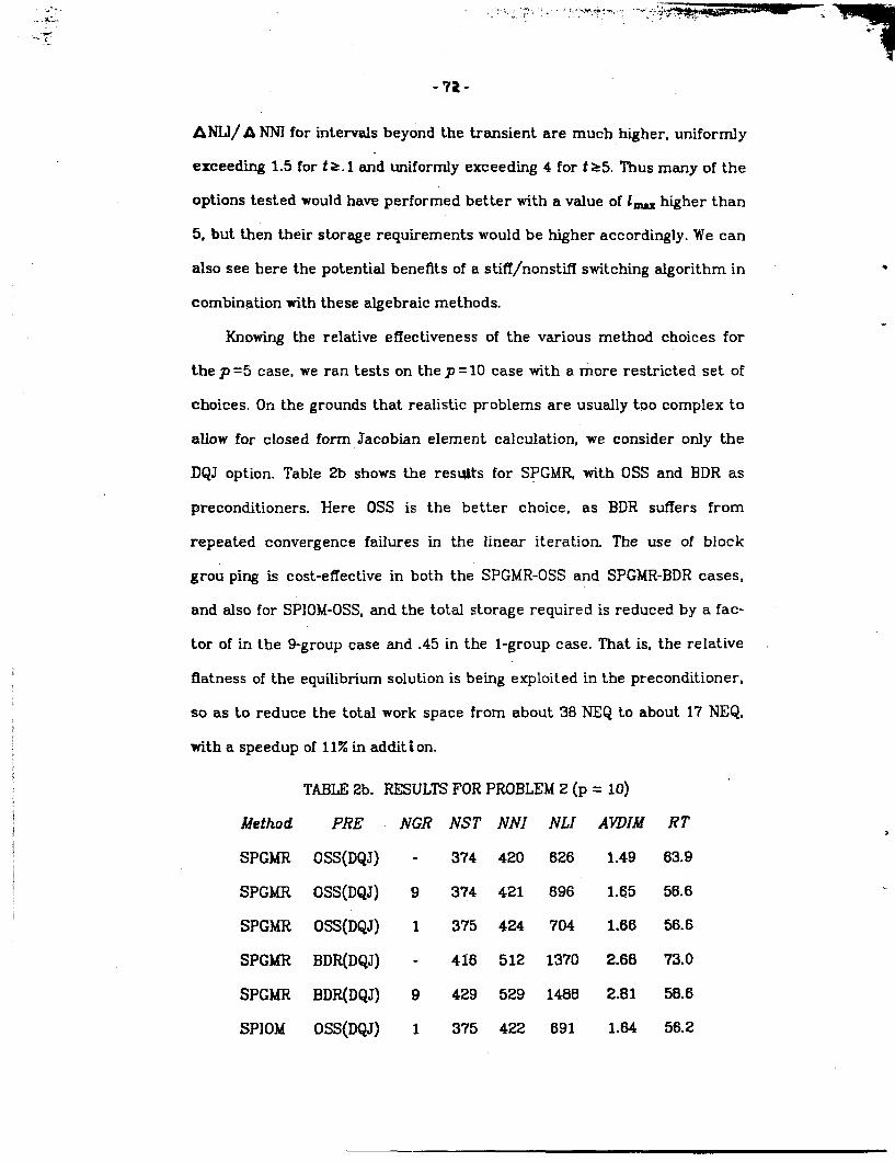
.. , :.,? . f ! . ..wy.!% ... . ‘“””.-’ij&?&?@m- .

‘7 *-7a-

ANLI/ A NNl for intervals beyond the transient are much hWher, uniformly

exceedhg 1.5 for fs. 1 and uniformly exceeding 4 for f >5. Thus many of the

options tested would have performed better with a value of 1- Klgher than

5, but then their storage requirements would be h~her accordhgly. We can

also see here the potential benefits of a .stiff/nonstiff switching algorithm in

combh@.ion with these algebraic! methods.

Knowing the relative effectiveness of the various method choices for

the p =5 case, we ran tests on the p = 10 case with a more restricted set of

choices. On the grounds that realistic problems are usually too complex to

allow for closed form Jacobian element calculation, we consider only the

DQJ option. Table 2b shows the resi$ts for SPGMR, with 0SS and BDR as

preconditioners. Here 0SS is the better choice, as BDR suffers from

rep”eated convergence failures in the linear iteration. The use of block

grou ping is cost-effective in both the SPGMR-OSS and SPGMR-BDR cases,

and also for SPIOM-OSS, and the total storage required is reduced by a fac-

tor of in the 9-group case and .45 in the l-group case. That is, the relative

flatness of the equilibrium solution is being exploited in the preconditioned,

so as to reduce the total work space from about 38 NEQ to about 17 NEQ,

with a speedup of 11% in addlt I on.

TABLEZb. RESULTSFOR PROBLEM2 (p = 10)

Method PRE NGR NST NNI NLI AKDIM

SPGMR OSS(I)QJ) - 374 420 626 1.49

SPGMR OSS(DQJ) 9 374 421 696 1.65

SPGMR OSS(DQJ) 1 375 424 704 1.66

SPGMR BDR(DQJ) - 416 512 1370 2.60

SPGMR BDR(DQJ) 9 429 529 1480 2.81

SPIOM OSS(DQJ) 1 375 422 691 1.64

RT

63.9

56.6

56.6

73.0

58.6

56.2

>

. ..- .--!

-73-

*

I

*

*

fd) Test Problem 3 .

The parameters in Problem 2 are such that the solution is rather fiat

spatially over the stiff part of the problem. In order to obtain a more realistic

situation, the problem can be made much more inhomogeneous spatially by

increasing the parameter a in the interaction coefficients bi in (6.5). For Prob-

lem 3, we take a=50, leaving all other problem parameters unchanged from

Problem 2. We consider the same two cases, p =5 and p =10 , with the same ini-

tial conditions and discret,ization (on a 12x12 mesh). The solution now shows a

spread in each c* by a factor of up to 5.2 at equilibrium, and equilibrium is

reached somewhat sooner.

Table 3a contains results for this problem in the 10-species case (p=5).

The runs with SIOM (no preconditioning) and with SPGMR-SOR failed to finish

after 1 minute and so were stopped. Clearly this problem requires a precondi-

tioning that includes the interaction Jacobian. All cases in the table are for

user-supplied Jacobian elements; all our data suggests that the DQJ results

would show a similar preference order. The 0SS preconditioned was faster than .

OSF, as in Problem 2, but here both were slower than the IOJ (interaction-only)

preconditioned. The diffusion apparently contributes less (relatively) to the

stiffness, so that dropping the SOR preconditioning at the cost of a somewhat

higher average Krylov dimension seems to be a good tradeoff in terms of total

cost. The BDL and BDR (block-diagonal) preconditioners perform much like IOJ,

with BDR sliihtly faster. Thus the inclusion of the diagonal transport coefficient

has little effect on either NLI or the run time, when there is no block grouping.

Block grouping is effective with both IOJand BDIL but less so for IOJ; the reasons

for the higher NU there are not clear. For BDR, there is also evidence that using

fewer than 16 groups is probably unwise. The considerable inhomogeneity of the

equilibrium solutilon and the moderate amount of diffusion (though not dom-

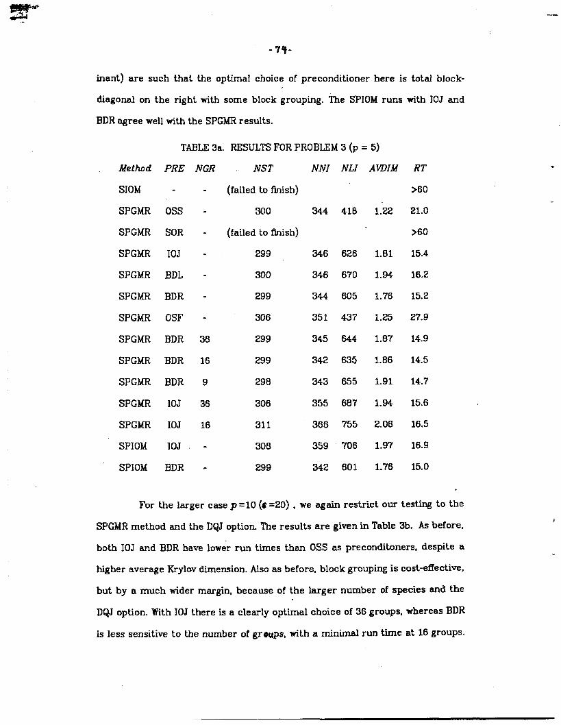
3!&-.. -----

inant) are such

diagonal on the

-79-

that the optimal choice of preconditioned here is tobd block-

right with some block grouping. The SP1OMruns with IOJ and

BDR agree well with the SPGMRresults.

TABLE3a. RESULTSFOR PROBLEM3 (p = 5)

Method

S1OM

SPGMR

SPGMR

SPGMR

SPGMR

SPGMR

SPGMR

SPGMR

SPGMR

SPGMR

SPGMR

SPGMR

SPIOM

SPIOM

PRE

0ss

SOR

IOJ

BDL

BDR

OSF

BDR

BDR

BDR

IOJ

IOJ

IOJ

BDR

NGR

.

36

16

9

36

16

NST

[failed to tlnish)

300

(failed to finish)

299

300

299

306

299

299

298

306

311

306

299

NNI

344

346

346

351

345

342

343

355

366

359

342

NLI

418

626

670

6115

437

644

635

655

687

755

706

601

AVDIM

1:22

1.81

1.94

1.76

1.25

1.87

1.86

1.91

1.94

2.06

1.97

1.76

RT

>60

21.0

>60

15.4

16.2

15.2

27.9

14.9

14.5

14.7

15.6

16.5

16.9

15.0

For the larger case p =10 (S =20) , we again restrict our testi to the

SPGMR method and the DQJ option. The results are given in Table 3b. As before,

both IOJ and BDR have lower rw times than 0SS as precondltoners, despite a

higher average Krylov dmension. Also as before, block grouping is cost-effective,

but by a much wider margin, because of the larger number of species and the

.

DQJ option. With IOJ there is a clearly optimal choice of 36 groups, whereas BDR

is less sensitive to the number of groups, with a minimal run time at 16 groups.

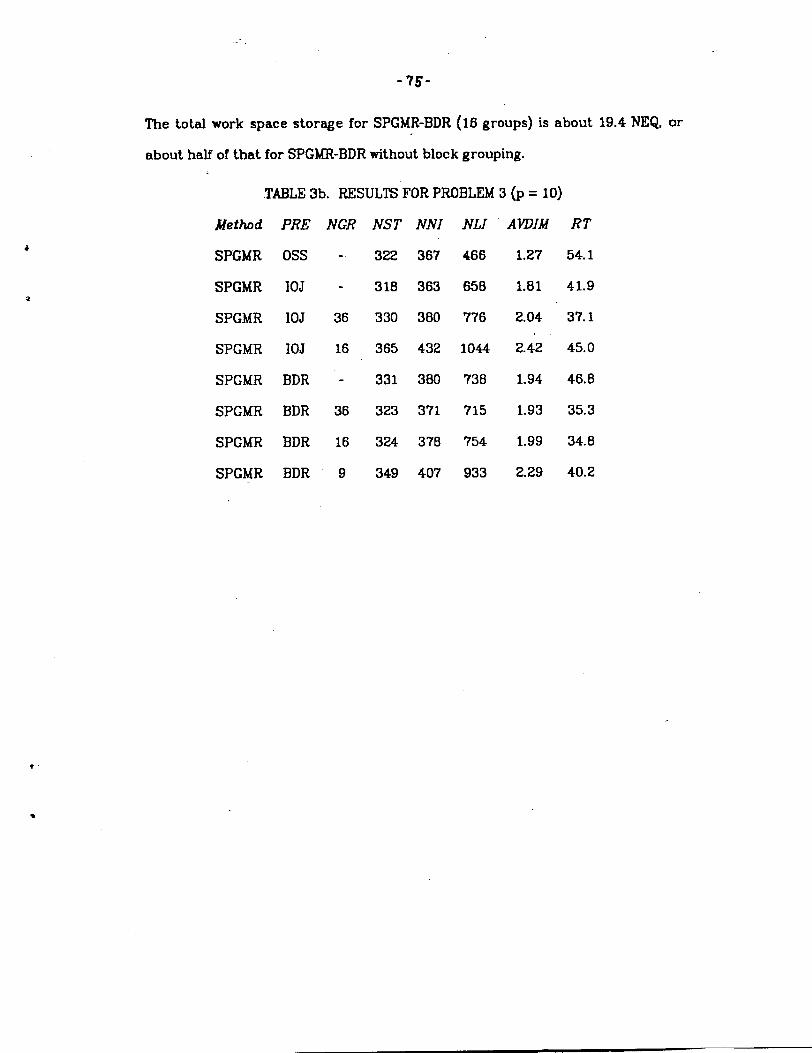
-?s -

The total work space storage for SPGMR-BDR (16 groups) is about 19.4 NEQ, or

about half of that for SPGMR-BDRwithout block grouping.

TABLE3b. RESULTSFOR PROBLEM3 (p = 10)

Method

SPGMR

SPGMR

SPGMR

SPGMR

SPGMR

SPGMR

SPGMR

SPGMR

PRE

0ss

IOJ

IOJ

IOJ

BDR

BDR

BDR

BDR

NGR NST NNI

322 367

318 363

36 330 380

16 365 432

331 380

36 323 371

16 324 378

9 349 407

NLI

466

658

776

1044

738

715

754

933

AVDIM RT

1.27 54.1

1.81 41.9

2.04 37.1

2.42 45.0

1.94 46.8

1.93 35.3

1.99 34.8

2.29 40.2

-76-

7. Conclusion

Krylov subspace iteration methods for linear systems can be combined

with Newton iteration and the BDF method to obtain effective algorithms for stiff

ODE systems. We have shown how the Arnoldi/10M, GMRES, and CG methods fit

into such combinations, and provided some theoretical support for the com-

bined liiear~nonlinear iteration when a finite-difference approximation is used

for the linear operator. We have also given algorithms for these methods that

include both scaling and preconditioning, and implemented these in an experi-

mental solver called LSODPK.

For some problems,

basic iteration methods with

problems. preconditioning is

mainly those with much spectral clustering, the

only scaling added are sufhcient. But for most

necessary to achieve robustness. We have con-

structed several preconditioned combinations for reaction-diffusion probIems,

US-W the reaction and transport operators indhridually, or in combination as in

operator splittlng, and using grouping of blocks of Jacobian elements involved to

achieve both storage and computational economies.

The tests we have reported show that these methods are effective on at

least a small set of test problems. The optimal choices of method combinations

depend on the nature of the problem, and may not be clear without experimen-

tation. Preconditioning based on operator splitting does well on most of PDE-

based problems we tested, but not ail. For some cases, where diffusion and

interaction terms are both equally dominant in the stiff part of the problem, we

found that neither the splitting approach nor one using either operator alone

seemed to do well. In general, we found that SPGMR is slightly preferable to

SPIOM, but that on probIems where a syrqmetry assumption is true or approxi-

mately true, PCG or SPCG can be more effkient. The same is probably true for

the GCR (Generalized Conjugate Residual) method, although we have not

*

-7?-

included that method in our testing.

There are other types of preconditioners in use elsew!,ere that we have

not yet studied, but which might prove useful in connection with the methods

used here. These include block-SOR (which has had considerable success by

itseIf within BDF solvers), incomplete LU or modified forms thereof (MILU), poly-

nomial preconditioners (e.g. Chebyshev), and Quasi-Newton (based on rank- one

matrix updates). The block-di agonal precondi ti oners would benefit greatlyfrom a dynamic group selection scheme.

Finally, we hope to see these methods extended to other types of stiff

ODE methods (e.g. implicit R.K), and to implicit forms of ODE’s (e.g. A$ =g, or

fully implicit systems), and to differential-algebraic equations.

.78-

REFERENCES

[1]

[2]

[3]

[4]

[5]

[6]

[7]

[8]

[9]

[10]

[11]

[12]

[13]

[14]

W. E. Arnoldi, The Principle of Minimized Iterations in the Solutionof the Matrix Eigenvalue Problem, Quart. J. A@. Math., 9 (1951),pp. 17-29.

P. N. Brmm, A -l Convergence Theory for Cabined InexactNewton\Finlte-Difference Projection Methods, to a~ar in SUM J.Num. Anal.

P. N. Brown, Decay to uniform States in Food Webs, SIAMJ. APP1.Math. 46 (1986), pp. 376-392.

P. N. Brown and A. C. Hhdnarsh, Matrix-Free Methods for StiffSystem of ODEs,SIAMJ. Num.Anal.,23 (1986),pp. 610-638.

T. F. Chan and K. R. Jackson, The Use of Iterative Linear EquationSolvers in Codes for Large Systems of Stiff IVPS for ODES,SIAM J.Sci. Stat. Ccmp., 7 (1986),pp. 378-417.

R. S. lX@o, S. C. Eisenstat and T. Steihaug, Inexact NewtonMethods, SIAMJ. Num. Anal., 19 (1982), pp. 400-408.

J. E. Dennis,Jr. and R. B. Schnabel, IWmrical I’4thods forUnconstrained Q timization and Nonlinear Equations, Pren=m-HallSeries in Computational Mati~mticsr 1983.

S. C. Eisenstat,H. C. Elman and M. H. Schultz, Variational Methodsfor Nonsymmetric System of Linear ~atbns, SIPM J. Num. Anal., 20(1983) , pp. 345-357.

C. W. Gear and Y. Saad, Iterative Solution of Linear Equations inOLE Codes, S12MJ. Sci. Stat. Comp., 4 (1983), ~. 583-601.

G. H. Goluband C. F. Van Loan,MatrixComPUtations,JohnsHopkinsUniversityPress,Baltimore,1983.

M. R. Hestenes and E. Stiefel, bksthods of conjugate Gradient forSolving Linear Systems, J. of Res. of the Nat’1 Bur. of Stan., 49(1952) , pp. 409-436.

A. C. Hindmarsh,Preliminary Documentation of GEARBI: Solution ofODE Systemswith Block-Iterative Treatment of the Jacobian, LINLReport uCID-30149, December 1976.

A. C. Hindmarsh,ISODEand ISODI,Two New InitialValueOrdinaryDifferentialFquationSolvers,in ACM Newsletter,Vol. 15, No. 4(December1980),pp. 10-11.

A. C. Hindmarsh,ODEPACK,A SystematizedCollectionof ODE Solvers,in ScientificCcmputing,R. S. Stepleman,et al. (eds.),North-Holland,Amsterdamr1983,pp. 55-64.

-79-

[15] W. L. Miranker and I-L. Chern, Dichotany and Conjugate Gradients inthe Stiff Initial Value FYoblem J. Lin. Alg. A@., 36 (1981), pp.57-77.

[16] Y. Saad, Variations on Arnoldi’s Method for ComputingEigenelementsof Iarge Unsynmtric Matrices, J. Lin. Alg. A@., 34 (1980)~ pp.269-295.

8

[17] Y. Saad,KrylovSubspacehkthodsfor Solving Large Unsyn’tnetricLinear Systems, wth. Conp.f 37 (1981), pp. 105-126.

[181 Y. Saad, practical Use of Sane Krylov Subspace Methods for SolvingItiefiniteand NonsymnetricLinearSystems,SIAM J. Sci. Stat.q=, 5 (1984),pp. 203-228.

[19] Y. Saad and M. H. Schultz,QWWS: A GeneralizedMinimal.ResidualAlgorithmfor SolvingNonsymnetricLinearSystms, Yale Univ.Dept.of Crop.Sci. ‘Ibch.ReportYALEU/bCS/RR-254,August1983.

[20] P. N. Swartztrauberand R. A. Sweet,Algorithm541:EfficientFbrtranSubprogramsfor the Solutionof SeparableEllipticPartialDifferential~tions, ZOl Trans.Math.Softw.t5 (1979)8pp.352-364.