Circular Polarization Feed for Space Communication on the 3 cm Band Part 1

Rastislav Galuscak1- OM6AA, Bert Modderman - PE1RKI, Vladimir Masek - OK1DAK, Pavel Hazdra1,Milos Mazanek1, Jeffrey Pawlan – WA6KBL

1 Czech Technical University, Department of Electromagnetic Field, FEE, Prague, Technicka 2, 166 27, Czech Republic, om6aa@yahoo.com

Introduction

While circular polarization (CP) is widely accepted among Earth-Moon-Earth (EME) station operators using the 23, 13, 9 and 6 cm bands, the use of CP on the 3 cm band (10 GHz) remains under discussion [1]. Polarization mismatch losses at 10 GHz caused by Faraday rotation are almost negligible; whereas, a one-way transversal through the atmosphere twists the polarization vector about 108° at 1GHz. At 10 GHz it is only 1.1° [2]. Reasons for favoring linear polarization (LP) on 3 cm are because of the relatively complex antenna and depolarization issues associated with CP and the availability of various surplus MW components suitable for ham radio EME linear polarization applications.

1. Depolarization of EME signals

1.1 Atmospheric depolarization

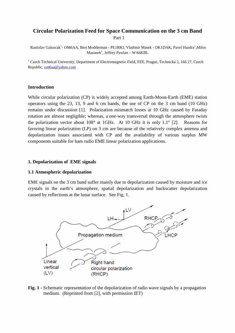
EME signals on the 3 cm band suffer mainly due to depolarization caused by moisture and ice crystals in the earth’s atmosphere, spatial depolarization and backscatter depolarization caused by reflections at the lunar surface. See Fig. 1.

Fig. 1 - Schematic representation of the depolarization of radio wave signals by a propagation medium. (Reprinted from [2], with permission IET)

To better quantify the problem, the Cross-Polarization Discrimination Term, XPD, is introduced and defined as:

[1]

Where: Ecross is the Electric Field Cross-Polarization Component Phasor Eco is the Electric Field Co-Polarization Component Phasor XPD is expressed in positive decibels

For circular polarization, using the axial ratio:

[2]

Where: axial ratio, r, is the ratio of the polarization elipse’s major to minor axis of polarization of the electric field vector, and Axial Ratio [dB] = 20log r

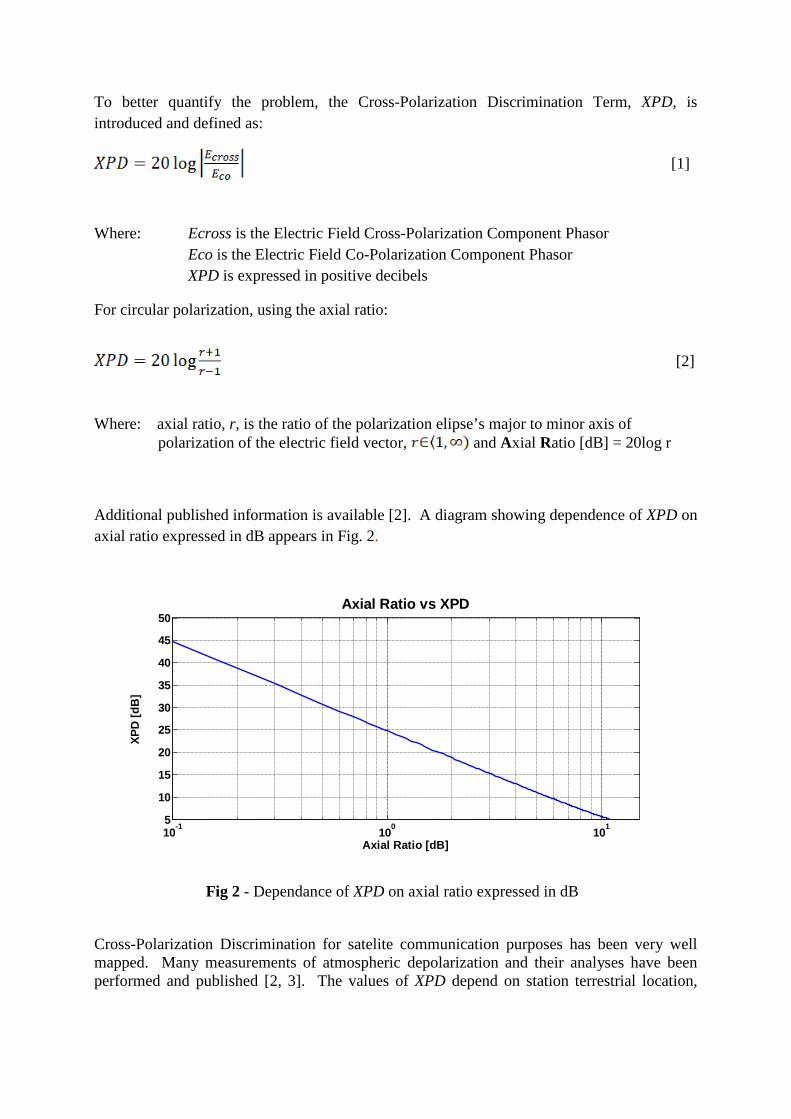
Additional published information is available [2]. A diagram showing dependence of XPD on axial ratio expressed in dB appears in Fig. 2.

10-1 100 1015

10

15

20

25

30

35

40

45

50

Axial Ratio [dB]

XPD

[dB

]

Axial Ratio vs XPD

Fig 2 - Dependance of XPD on axial ratio expressed in dB

Cross-Polarization Discrimination for satelite communication purposes has been very well mapped. Many measurements of atmospheric depolarization and their analyses have been performed and published [2, 3]. The values of XPD depend on station terrestrial location,

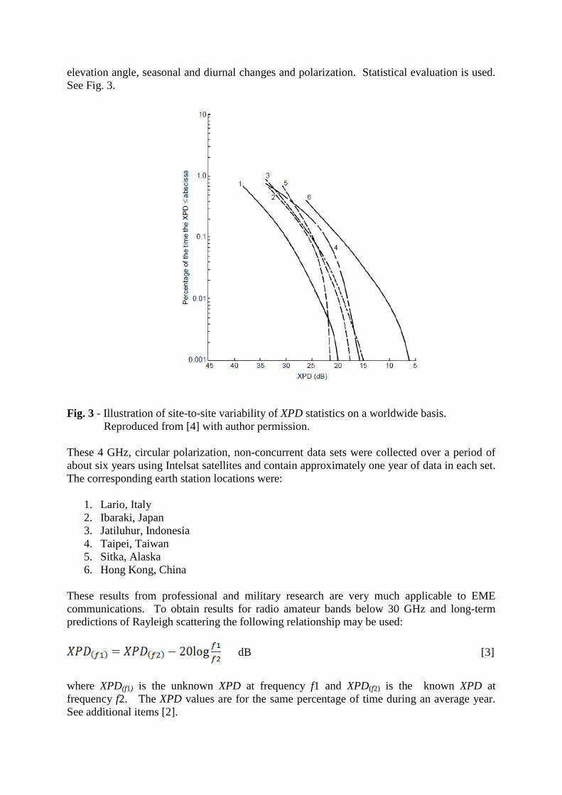
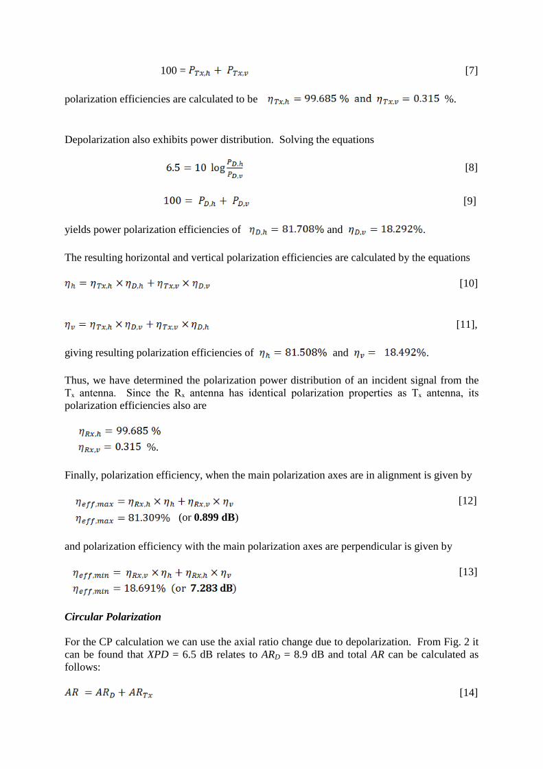
elevation angle, seasonal and diurnal changes and polarization. Statistical evaluation is used. See Fig. 3.

Fig. 3 - Illustration of site-to-site variability of XPD statistics on a worldwide basis. Reproduced from [4] with author permission. These 4 GHz, circular polarization, non-concurrent data sets were collected over a period of about six years using Intelsat satellites and contain approximately one year of data in each set. The corresponding earth station locations were:

1. Lario, Italy 2. Ibaraki, Japan 3. Jatiluhur, Indonesia 4. Taipei, Taiwan 5. Sitka, Alaska 6. Hong Kong, China

These results from professional and military research are very much applicable to EME communications. To obtain results for radio amateur bands below 30 GHz and long-term predictions of Rayleigh scattering the following relationship may be used:

dB [3]

where XPD(f1) is the unknown XPD at frequency f1 and XPD(f2) is the known XPD at frequency f2. The XPD values are for the same percentage of time during an average year. See additional items [2].

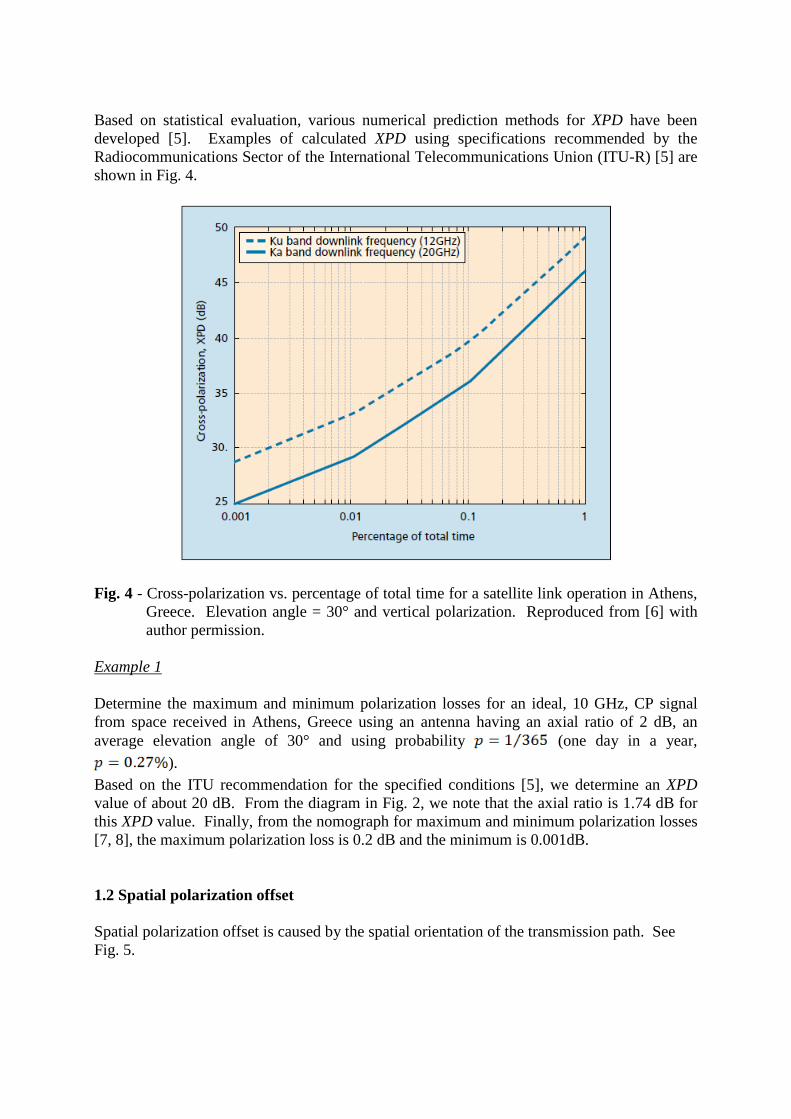
Based on statistical evaluation, various numerical prediction methods for XPD have been developed [5]. Examples of calculated XPD using specifications recommended by the Radiocommunications Sector of the International Telecommunications Union (ITU-R) [5] are shown in Fig. 4.

Fig. 4 - Cross-polarization vs. percentage of total time for a satellite link operation in Athens, Greece. Elevation angle = 30° and vertical polarization. Reproduced from [6] with author permission. Example 1 Determine the maximum and minimum polarization losses for an ideal, 10 GHz, CP signal from space received in Athens, Greece using an antenna having an axial ratio of 2 dB, an average elevation angle of 30° and using probability (one day in a year,

). Based on the ITU recommendation for the specified conditions [5], we determine an XPD value of about 20 dB. From the diagram in Fig. 2, we note that the axial ratio is 1.74 dB for this XPD value. Finally, from the nomograph for maximum and minimum polarization losses [7, 8], the maximum polarization loss is 0.2 dB and the minimum is 0.001dB. 1.2 Spatial polarization offset Spatial polarization offset is caused by the spatial orientation of the transmission path. See Fig. 5.

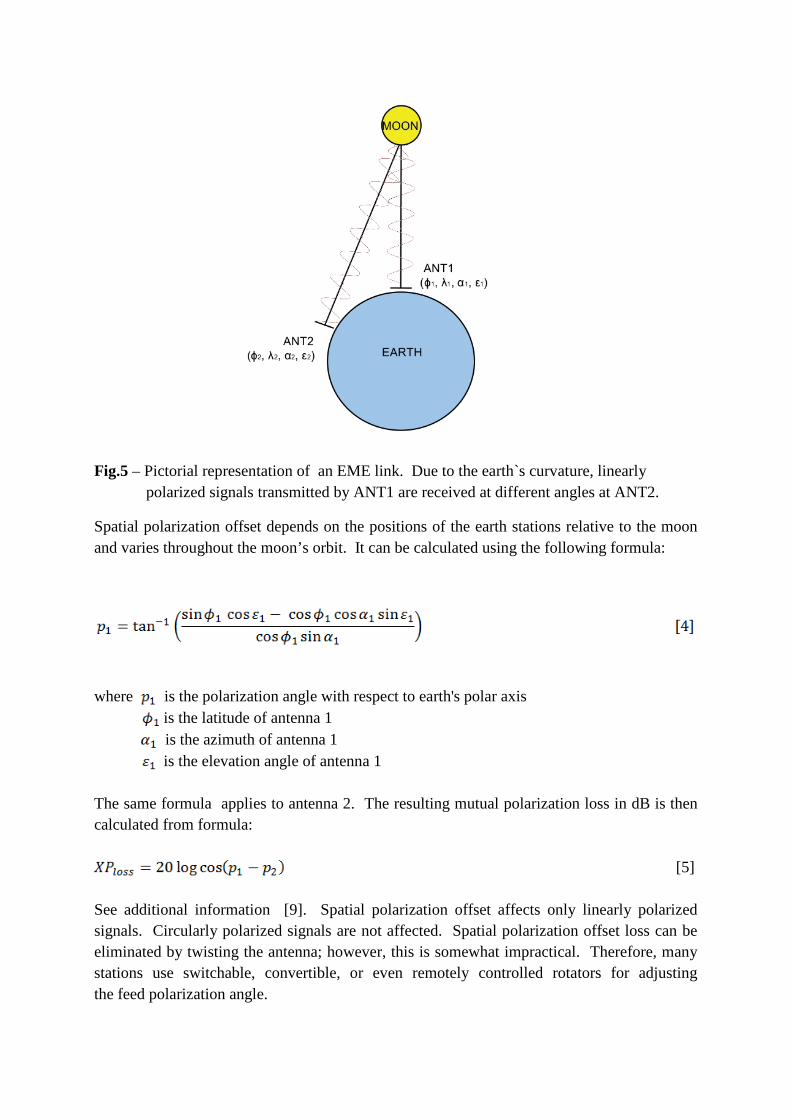
Fig.5 – Pictorial representation of an EME link. Due to the earth`s curvature, linearly polarized signals transmitted by ANT1 are received at different angles at ANT2.

Spatial polarization offset depends on the positions of the earth stations relative to the moon and varies throughout the moon’s orbit. It can be calculated using the following formula:

where is the polarization angle with respect to earth's polar axis is the latitude of antenna 1 is the azimuth of antenna 1 is the elevation angle of antenna 1 The same formula applies to antenna 2. The resulting mutual polarization loss in dB is then calculated from formula:

[5] See additional information [9]. Spatial polarization offset affects only linearly polarized signals. Circularly polarized signals are not affected. Spatial polarization offset loss can be eliminated by twisting the antenna; however, this is somewhat impractical. Therefore, many stations use switchable, convertible, or even remotely controlled rotators for adjusting the feed polarization angle.

1.3 Backscatter Depolarization

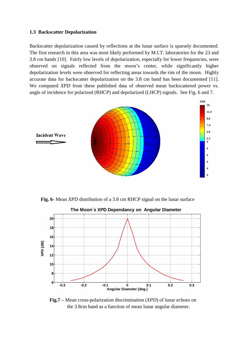
Backscatter depolarization caused by reflections at the lunar surface is sparsely documented. The first research in this area was most likely performed by M.I.T. laboratories for the 23 and 3.8 cm bands [10]. Fairly low levels of depolarization, especially for lower frequencies, were observed on signals reflected from the moon’s center, while significantly higher depolarization levels were observed for reflecting areas towards the rim of the moon. Highly accurate data for backscatter depolarization on the 3.8 cm band has been documented [11]. We computed XPD from these published data of observed mean backscattered power vs. angle of incidence for polarized (RHCP) and depolarized (LHCP) signals. See Fig. 6 and 7.

Fig. 6- Mean XPD distribution of a 3.8 cm RHCP signal on the lunar surface

-0.3 -0.2 -0.1 0 0.1 0.2 0.36

8

10

12

14

16

18

20

Angular Diameter [deg.]

XPD

[dB

]

The Moon`s XPD Dependancy on Angular Diameter

Fig.7 – Mean cross-polarization discrimination (XPD) of lunar echoes on the 3.8cm band as a function of mean lunar angular diameter.

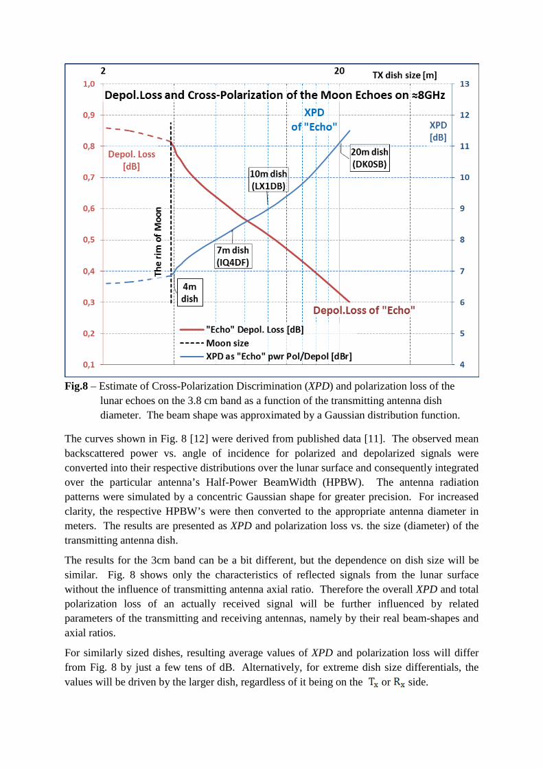
Fig.8 – Estimate of Cross-Polarization Discrimination (XPD) and polarization loss of the lunar echoes on the 3.8 cm band as a function of the transmitting antenna dish diameter. The beam shape was approximated by a Gaussian distribution function.

The curves shown in Fig. 8 [12] were derived from published data [11]. The observed mean backscattered power vs. angle of incidence for polarized and depolarized signals were converted into their respective distributions over the lunar surface and consequently integrated over the particular antenna’s Half-Power BeamWidth (HPBW). The antenna radiation patterns were simulated by a concentric Gaussian shape for greater precision. For increased clarity, the respective HPBW’s were then converted to the appropriate antenna diameter in meters. The results are presented as XPD and polarization loss vs. the size (diameter) of the transmitting antenna dish.

The results for the 3cm band can be a bit different, but the dependence on dish size will be similar. Fig. 8 shows only the characteristics of reflected signals from the lunar surface without the influence of transmitting antenna axial ratio. Therefore the overall XPD and total polarization loss of an actually received signal will be further influenced by related parameters of the transmitting and receiving antennas, namely by their real beam-shapes and axial ratios.

For similarly sized dishes, resulting average values of XPD and polarization loss will differ from Fig. 8 by just a few tens of dB. Alternatively, for extreme dish size differentials, the values will be driven by the larger dish, regardless of it being on the or side.

Note that XPD for dishes with diameter below 4 meters can be expected to be about 6.5dB.

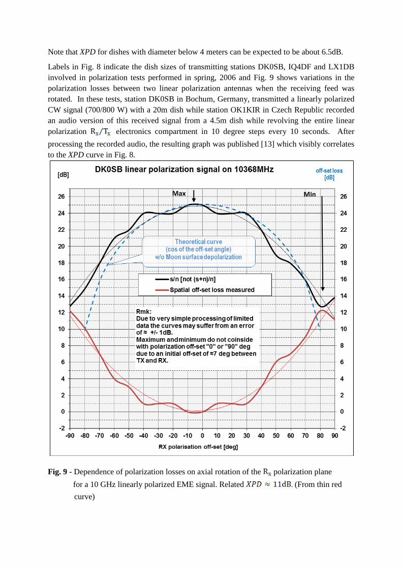
Labels in Fig. 8 indicate the dish sizes of transmitting stations DK0SB, IQ4DF and LX1DB involved in polarization tests performed in spring, 2006 and Fig. 9 shows variations in the polarization losses between two linear polarization antennas when the receiving feed was rotated. In these tests, station DK0SB in Bochum, Germany, transmitted a linearly polarized CW signal (700/800 W) with a 20m dish while station OK1KIR in Czech Republic recorded an audio version of this received signal from a 4.5m dish while revolving the entire linear polarization electronics compartment in 10 degree steps every 10 seconds. After processing the recorded audio, the resulting graph was published [13] which visibly correlates to the XPD curve in Fig. 8.

Fig. 9 - Dependence of polarization losses on axial rotation of the polarization plane

for a 10 GHz linearly polarized EME signal. Related . (From thin red curve)

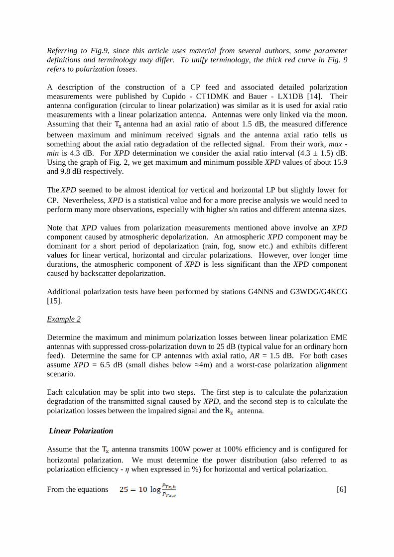
Referring to Fig.9, since this article uses material from several authors, some parameter definitions and terminology may differ. To unify terminology, the thick red curve in Fig. 9 refers to polarization losses. A description of the construction of a CP feed and associated detailed polarization measurements were published by Cupido - CT1DMK and Bauer - LX1DB [14]. Their antenna configuration (circular to linear polarization) was similar as it is used for axial ratio measurements with a linear polarization antenna. Antennas were only linked via the moon. Assuming that their antenna had an axial ratio of about 1.5 dB, the measured difference between maximum and minimum received signals and the antenna axial ratio tells us something about the axial ratio degradation of the reflected signal. From their work, max - min is 4.3 dB. For XPD determination we consider the axial ratio interval (4.3 ± 1.5) dB. Using the graph of Fig. 2, we get maximum and minimum possible XPD values of about 15.9 and 9.8 dB respectively. The XPD seemed to be almost identical for vertical and horizontal LP but slightly lower for CP. Nevertheless, XPD is a statistical value and for a more precise analysis we would need to perform many more observations, especially with higher s/n ratios and different antenna sizes. Note that XPD values from polarization measurements mentioned above involve an XPD component caused by atmospheric depolarization. An atmospheric XPD component may be dominant for a short period of depolarization (rain, fog, snow etc.) and exhibits different values for linear vertical, horizontal and circular polarizations. However, over longer time durations, the atmospheric component of XPD is less significant than the XPD component caused by backscatter depolarization. Additional polarization tests have been performed by stations G4NNS and G3WDG/G4KCG [15]. Example 2 Determine the maximum and minimum polarization losses between linear polarization EME antennas with suppressed cross-polarization down to 25 dB (typical value for an ordinary horn feed). Determine the same for CP antennas with axial ratio, AR = 1.5 dB. For both cases assume XPD = 6.5 dB (small dishes below ≈4m) and a worst-case polarization alignment scenario. Each calculation may be split into two steps. The first step is to calculate the polarization degradation of the transmitted signal caused by XPD, and the second step is to calculate the polarization losses between the impaired signal and antenna. Linear Polarization Assume that the antenna transmits 100W power at 100% efficiency and is configured for horizontal polarization. We must determine the power distribution (also referred to as polarization efficiency - η when expressed in %) for horizontal and vertical polarization. From the equations [6]

100 = [7] polarization efficiencies are calculated to be %. Depolarization also exhibits power distribution. Solving the equations [8]

[9] yields power polarization efficiencies of and . The resulting horizontal and vertical polarization efficiencies are calculated by the equations

[10]

[11], giving resulting polarization efficiencies of and . Thus, we have determined the polarization power distribution of an incident signal from the Tₓ antenna. Since the Rₓ antenna has identical polarization properties as Tₓ antenna, its polarization efficiencies also are

%. Finally, polarization efficiency, when the main polarization axes are in alignment is given by [12] (or 0.899 dB) and polarization efficiency with the main polarization axes are perpendicular is given by [13] Circular Polarization For the CP calculation we can use the axial ratio change due to depolarization. From Fig. 2 it can be found that XPD = 6.5 dB relates to ARD = 8.9 dB and total AR can be calculated as follows:

[14]

dB Since dB our task is to determine maximum and minimum polarization losses between these CP antennas with AR = 10.4 and 1.5 dB. Using the published nomograph [7, 8], minimum and maximum polarization losses are found to be 0.61 and 1.34 dB respectively. It has been shown that despite atmosphere and backscatter depolarization, CP exhibits high polarization efficiency. In addition, CP does not suffer with spatial polarization offset. Based on these findings and works published by others [1,14], we believe that it is advantageous to also use CP on the 3 cm (10 GHz) band. To provide new solutions for active EME stations utilizing the beneficial properties of CP, a cascaded square-to-circular cross section waveguide having a septum polarizer located within the square waveguide is described in Part 2 of this article. This CP feed is applicable to both prime focus and offset parabolic antenna configurations. Acknowledgements We would like to express our thanks to the operators of active 3 cm band EME stations, Prof. Miroslav Kasal - OK2AQ and Mr. Frantisek Strihavka - OK1CA, for their technical consultation. Additionally, we would like to thank Mr. Robert Valenta for language and technical assistance. References for part 1 [1] Marko Cebokli-S57UUU „Let's go circular on 10” 9th EME conference, Rio de Janeiro 2000, available online at: http://lea.hamradio.si/~s57uuu/emeconf/ltsgocir.htm [2] Allnut J.E. „Satellite-to-ground radiowave propagation” 2d ed. IET publication 2011, London, United Kingdom, ISBN 978-1-84919-150-0 [3] Dalgleish, D.I. „An introduction to satellite communications” IEE publication 1991, Peter Peregrinus Ltd., London, United Kingdom, ISBN 0-86341-132-0 [4] Allnut J.E. „The system implications of 6/4 GHz satellite-to-ground signal depolarization results from the INTELSAT propagation measurements programme” Int. J. Satellite Commun., 1984, vol. 2, pp. 73–80. [5] Recommodation ITU-R P.618-11, 6/2013 „Propagation data and prediction methods required for the design of Earth-space telecommunication systems” available online at: http://www.itu.int/ITU-R/go/patents/en [6] Panagopoulos Athanasios D, M. Arapoglou Pantelis-Daniel and G. Cottis Panayotis „Satellite Communications at KU,KA and V Bands: Propagation Impairments and Mitigation Techniques” IEEE Communications Surveys, Third Quarter 2004, Volume 6, No. 3 [7] Milligan, T. A. „Modern Antenna Design” Wiley-IEEE Press, 2nd edition, July 11, 2005.

ISBN-13 978-0-471-45776-3 [8] Galuscak Rastislav, Hazdra Pavel, „Circular Polarization and Polarization Losses”, DUBUS, 4/2006, ISSN 1438-3705

[9] Kelly Paul –N1BUG, „Polarization of EME Signals: How to Succeed More Often” available online at: http://www.g1ogy.com/www.n1bug.net/operate/emepol-1.html

[10] Tor Hagfors, „A Study of the Depolarization of Lunar Radar Echoes” Radio Science, Vol. 2 (new series) No. 5, May 1967, available online at: http://www.wa5vjb.com/moon.html [11] S.H.Zisk et al., "High-resolution Radar Maps Of The Lunar Surface At 3.8cm Wavelength", The Moon, 10 (1974),pp.17-50

[12] Masek Vladimir – OK1DAK, private paper [13] Jelinek Antonin - OK1DAI, Masek Vladimir - OK1DAK, „24 GHz EME at OK1KIR”, EME and MW seminar Studnice, Czech Republic April 2014, available online at: http://www.vhf.cz/soubory/dokumenty/eme-24-ghz-ok1kir-2014.pdf [14] Cupido, Luis-CT1DMK and Bauer, Willi-LX1DB, „Circular Polarized Antenna Feed for EME on 10 GHz and 5,7 GHz, ” DUBUS, 2/ 2006, ISSN 1438-3705, available online at: http://www.qsl.net/ct1dmk/cp_feed_dmk06.pdf

[15] Suckling Charlie - G3WDG, 10 GHz EME Polarization Tests, Jan. 2010 , available online at: http://www.sucklingfamily.free-online.co.uk/10GHzeme/10ghz_eme_polarization _tests.htm