arX

iv:1

810.

0423

3v2

[qu

ant-

ph]

11

Jan

2019

Trading locality for time: certifiable randomness from low-depth

circuits

Matthew Coudron ∗ Jalex Stark † Thomas Vidick ‡

January 14, 2019

Abstract

The generation of certifiable randomness is the most fundamental information-theoretic task that

meaningfully separates quantum devices from their classical counterparts. We propose a protocol for

exponential certified randomness expansion using a single quantum device. The protocol calls for the

device to implement a simple quantum circuit of constant depth on a 2D lattice of qubits. The output of

the circuit can be verified classically in linear time, and is guaranteed to contain a polynomial number of

certified random bits assuming that the device used to generate the output operated using a (classical or

quantum) circuit of sub-logarithmic depth. This assumption contrasts with the locality assumption used

for randomness certification based on Bell inequality violation and more recent proposals for randomness

certification based on computational assumptions. Furthermore, to demonstrate randomness generation

it is sufficient for a device to sample from the ideal output distribution within constant statistical distance.

Our procedure is inspired by recent work of Bravyi et al. (Science 2018), who introduced a relational

problem that can be solved by a constant-depth quantum circuit, but provably cannot be solved by any

classical circuit of sub-logarithmic depth. We develop the discovery of Bravyi et al. into a framework

for robust randomness expansion. Our results leads to a new proposal for a demonstrated quantum

advantage that has some advantages compared to existing proposals. First, our proposal does not rest on

any complexity-theoretic conjectures, but relies on the physical assumption that the adversarial device

being tested implements a circuit of sub-logarithmic depth. Second, success on our task can be easily

verified in classical linear time. Finally, our task is more noise-tolerant than most other existing proposals

that can only tolerate multiplicative error, or require additional conjectures from complexity theory; in

contrast, we are able to allow a small constant additive error in total variation distance between the

sampled and ideal distributions.

1 Introduction

A fundamental point of departure between quantum mechanics and classical theory is that the former is non-

deterministic: quantum mechanics, through the Born rule, posits the existence of experiments that generate

intrinsic randomness. This observation leads to the simplest and most successful “test of quantumness” to

have been designed and implemented: the Bell test [Bel64]. Far beyond its role as a test of the foundations of

quantum mechanics, the Bell test has become a fundamental building block in quantum information, from

protocols for quantum cryptography (e.g. device-independent quantum key distribution [Eke91, VV14])

∗University of Waterloo, Canada. mcoudron@gmail.com†University of California Berkeley, USA. jalex@cs.berkeley.edu‡California Institute of Technology, USA. vidick@cms.caltech.edu

1

to complexity theory (e.g. delegated quantum computation [RUV13], multiprover interactive proof sys-

tems [CHTW04]) and much more [BCP+14]. Yet, while a loophole-free implementation of a Bell test has

been demonstrated [HBD+15, GVW+15, SMSC+15] it remains a challenging experimental feat, which un-

fortunately leaves its promising applications wanting (here ”loophole-free” refers to a stringent set of experi-

mental standards which ensure that all required assumptions have been verified “beyond reasonable doubt”).

The increasingly powerful quantum devices that are being experimentally realized tend to be single-chip,

and do not have the ability to implement loophole-free Bell tests. The task of devising convincing “tests of

quantumness” for such devices is challenging.

Until recently the only proposal for such tests was the design of so-called “quantum supremacy ex-

periments” [HM17], which specify classical sampling tasks that can in principle be implemented by a

mid-scale quantum device, but cannot be simulated by any efficient classical randomized algorithm (un-

der somewhat standard computational assumptions [AC17, HM17]). These proposals share a number of

well-recognized limitations. Firstly, while the sampling part of the process can be done efficiently on a

quantum computer, verifying that the quantum computer is sampling from a hard distribution requires a

computational effort which scales exponentially in the number of qubits. Secondly, their experimental re-

alization is hindered by a generally poor tolerance to errors in the implementation, which is compounded

by the necessity to implement circuits with relatively large (say, at least√

N for an N × N grid) depth.

Combined with the resort to complexity-theoretic assumptions for which there is little guidance in terms

of concrete parameter settings (see however [DHKLP18]), this has led to an ongoing race in efficient sim-

ulations [CZX+18, HNS18, MFIB18]. Indeed, the proposals operate in a limited computational regime,

requiring a machine with, say, at least 50 qubits (to prevent direct clasical simulation) but at most 70 qubits

(so that verification can be performed in a reasonable amount of time) — leaving open the question of what

to do with a device with more than, say, 100 qubits. At a more conceptual level, the proposals are based on

computational tasks that appear arbitrary (such as the implementation of a random quantum circuit from a

certain class). In particular, they do not lead to any further characterization of the successful device, that

could be used to e.g. build a secure delegation protocol or even simply certify a simple property such as the

preparation of a specific quantum state or the implementation of a certain class of measurements.

We propose a different kind of experiment, or “test of quantumness”, for large but noisy quantum de-

vices, that is inspired from recent work of Bravyi et al. on the power of low-depth quantum circuits [BGK17].

Our test is applicable in a regime where the device has a large number of qubits, but may only have the abil-

ity to implement circuits of low (constant) depth, due e.g. to a limited gate fidelity. We argue that the

test overcomes the main limitations outlined above: it generates useful outcomes (certifiably random bits),

it is easily verifiable (in classical linear time), and it is robust to a small amount of error (it is sufficient

to generate outputs within constant statistical distance from the ideal distribution1). The test does not re-

quire any assumption from complexity theory, but instead considers a novel physical assumption (introduced

in [BGK17]): that the device implements a circuit whose depth is at most a small constant times the loga-

rithm of the number of qubits. Intuitively, this assumption trades off locality (as required by the Bell test) for

time (as measured by circuit depth). It is particularly well-suited to quantum devices for which the number

of qubits can be made quite large, but the gate fidelity remains low, limiting the depth of a circuit that can

be implemented. Informally, we show the following.

Theorem 1.1. Let N be an arbitrary integer and M = N2. There exists universl constants c, d > 0, a

distribution D on 0, 1M , and an efficiently verifiable relation R ⊆ 0, 1M × 0, 1M such that the

followinog holds. Let C be a (classical or quantum) circuit with gates of constant fan-in and depth D ≤1In fact, even less is needed; see the description of the protocol.

2

c log M such that the output of the circuit satisfies the relation non-negligibly often, i.e.

Prx∼D

[(x, C(x)) ∈ R

]= Ω

(M−1/10

).

Then C achieves exponential randomness expansion: a sample from D can be obtained using O(log2 M)uniformly random bits and outputs of the circuit must have Ω(Md) bits of entropy.

We refer to Theorem 6.7 for a precise statement. In particular, the output entropy is quantified using the

quantum conditional min-entropy, conditioned on the inputs to the circuit and quantum side information that

may be correlated with the initial state of the circuit. Note that the resulting test is far more robust than most

existing proposals, that require the output distribution to be multiplicatively close to the target distribution.

In contrast, in our case it is sufficient to hit a certain target (the relation R, that itself is very permissive) an

inverse polynomial fraction of the time!

Aside from the application to randomness expansion, Theorem 1.1 strengthens the main result of Bravyi

et al. [BGK17] in multiple ways. Bravyi et al. provide a relation such that for any classical circuit of

sufficiently low depth, there exists an input such that the circuit must return an output that satisfies the

relation with probability bounded away from 1. In contrast, we point out the existence of an efficiently

sampleable distribution on inputs such that, for any classical low-depth circuit, we know that on average over

the choice of an input the circuit returns an output that satisfies the relation with at most small probability.

While this improvement follows using a simple extension of the arguments in [BGK17], it is key to the

practical relevance of the scheme. In addition we make a further improvement and address the following

question left open in [BGK17]: how small can the maximum success probability of all low-depth classical

circuits (i.e. the “soundness”) be made?

Theorem 1.2 (Exponential soundness). Let N be an arbitrary integer and M = N2. There exists a distri-

bution D on 0, 1M and an efficiently verifiable relation R ⊆ 0, 1M × 0, 1M such that the following

holds, for universal constants c, c′ > 0:

• (Completeness) There exists a depth-3 geometrically local (in 2D) quantum circuit such that for any

input x in the support of D the circuit samples a y such that (x, y) ∈ R with probability 1.

• (Soundness) For any classical circuit of depth D ≤ c log N, the probability that (x, y) ∈ R, for

x ∼ D and y the output of the circuit on input x, is O(exp(−Nc′)).

Note that the improvement in soundness between our two results is enabled by the fact that in Theo-

rem 1.2 it is no longer the case that it is possible to sample from D using poly-logarithmically many bits.

Arguably, good soundness guarantees are crucial to a successful experimental demonstration: due to the

presence of noise the quantum device cannot be expected to succeed with probability arbitrarily close to 1,

so that the lower the performance of classical circuits, the lower the requirements on the quantum circuit as

well.

Discussion. We comment on the depth assumption that underlies our results, and their potential for a

practical demonstration of a quantum advantage (a.k.a. “quantum supremacy experiment”). The quantum

circuit required for a successful implementation of our task is relatively straightforward to implement. It can

be realized in three phases. A first, offline phase initializes EPR pairs (or three-qubit GHZ states) between

nearest-neighbor qubits on a 2D grid. In a second phase, each qubit is provided an input, according to which

either the qubit should be measured according to a single-qubit Pauli observable, or the qubit and one of its

neighbors should be measured in the Bell basis. Finally, in the third phase the measurement outcomes are

aggregated and verified using a simple classical linear-time computation.

3

In order to demonstrate a quantum advantage, the crucial requirement is that the second phase should

be implemented using a procedure that is “certified” to have low depth. Since this is a physical assumption,

it can never be rigorously proven. Nevertheless, it is possible to imagine experiments under which the

assumption would hold “beyond reasonable doubt”. We describe two such experiments.

In a first scenario, the verification of the depth constraint could be based on a calculation that takes into

account state-of-the-art clock speeds. The fastest classical processors operate at speeds of order 1GHz, so

that for an integer N, a circuit of depth d = log(N) takes time of order 10−9 log(N) seconds to implement.

In contrast, current gate times for, say, ion-trap quantum computers are of order 100 nanoseconds [SBT+18],

meaning that the quantum circuit realizing our task could be implemented in time roughly 10−7 seconds.

To observe a quantum advantage it is thus necessary to ensure log(N) ≫ 102, leading to an impractical

circuit size. However, a reasonable factor 10 improvement in the gate time for quantum gates could enable

a demonstration based on a grid of order 210 × 210 qubits. Although far beyond current capabilities, the

number is not beyond reach. Keeping in mind the extreme simplicity of the task to be implemented, it is not

unreasonable to hope that such circuits may exist within 5-10 years.

In the previous scenario we allowed both the classical and quantum procedures solving our task to do

so in a highly localized, single-chip fashion. The distributed nature of the task lends itself well to another

type of implementation, that would be more demanding for a classical adversarial behavior, and may thus

lead to a more practical demonstration of quantum advantage. Consider a network of constant-qubit devices

arranged in a N × N grid, such that devices may be separated by large (say, kilometric) distances. In the

first, offline phase the devices use nearest-neighbor quantum communication channels to distribute EPR

pairs. In the second phase, each device receives a classical input, performs a simple local measurement, and

returns a classical output (no communication is required). Our result implies that, to even approximately

reproduce the output distribution implemented by this procedure, a classical network would need to operate

in at least Ω(log N) rounds, where in each round a device can communicate with a constant number of

devices located at arbitrary locations in the network (the network need not be 2D: at each step, a device is

allowed to broadcast arbitrarily but can only receive information from a constant number of devices, whose

identity must be fixed ahead of time). Taking into account inevitable latency delays incurred in any such

network, this second scenario suggests that our task may lead to an interesting test for a future quantum

internet [WEH18].

Finally we comment on the fidelity requirement for the gates of a quantum circuit implementing our task.

Even though the circuit is only of constant depth, it is important that, along a typical path of length O(N)between two qubits in the N × N grid, none of the gates leads to an error. This means that per-gate fidelity

is required to be of order 1− O(1/N). For N of order 210, as suggested in the first scenario described

above, such fidelities are within reach. We also note that by changing the architecture of the circuit from a

2D grid to a 3D grid it may be possible to leverage existing protocols for entanglement distribution using

noisy resources [RBH05]. Unfortunately, this comes with the drawback of a challenging 3D architecture for

which there is no current implementation.

Proof idea. Our starting point is the key observation, made by Bravyi et al. [BGK17], that a sub-logarithmic

depth circuit made of gates with constant fan-in has a form of implied locality, where the “forward light-

cone” of most input vertices only includes a vanishing fraction of output vertices. In particular, two randomly

chosen input locations are unlikely to have overlapping lightcones. If the input to the circuit is non-trivial

in those two locations only, then the outputs in each input location’s forward lightcone are obtained by

a computation that depends on that input only. In other words, we have a reduction from classical, low-

depth circuits to two-party local computation that exactly preserves properties of the output. While the same

lightcone argument holds true for a quantum circuit, the quantum circuit has the ability of distributing entan-

4

glement across any two locations in depth 2, by executing a sequence of entanglement swapping procedures

in parallel. Thus the same reduction maps a quantum, low-depth circuit to a two-party local computation,

where the parties may perform their local computation on a shared entangled state. Since there are well-

known separations between the kinds of distributions that can be generated by performing local operations

on an entangled state, as opposed to no entanglement at all — this is precisely the scope of Bell inequalities

— Bravyi et al. have obtained a separation between the power of low-depth classical and quantum circuits.

We build on this argument in the following way. Our first contribution is to boost the argument in [BGK17]

from a worst-case to a “high probability” statement. Instead of showing that (i) for every classical circuit,

there is some choice of input on which the classical circuit will fail, and (ii) there is a quantum circuit that

succeeds on every input, we show that there exists a suitable distribution on inputs that is such that, (i) any

classical circuit fails with high probability given an input from the distribution, and (ii) there is a quantum

circuit that succeeds with high probability (in fact, probability 1) on the distribution. Second, we observe that

the construction in [BGK17] imposes constraints not only on classical low-depth circuits, but also on quan-

tum low-depth circuits; this observation enables the reduction to nonlocal games hinted at above. Finally,

we amplify the argument to show how a polynomial number of Bell experiments can be simultaneously

“planted” into the input to the circuit. This allows us to perform a reduction to a nonlocal game in which

there is a large number of players divided into pairs which each perform their own distinct Bell experiment.

By adapting techniques from the area of randomness expansion from nonlocal games [AFDF+18] we are

then able to conclude that any sub-logarithmic-depth circuit, classical or quantum, that succeeds on our in-

put distribution, must generate large amounts of entropy. Moreover, this guarantee holds even if the circuit

only correctly computes a sufficiently large but constant fraction of outputs for the games.

Related work. Two recent works investigate the question of certified randomness generation outside of

the traditional framework of Bell inequalities. In [BCM+18] randomness is guaranteed based on the com-

putational assumption that the device does not have sufficient power to break the security of post-quantum

cryptography. The main advantages of this proposal are that the assumption is a standard cryptographic as-

sumption, and that verification is very efficient. A drawback is the interactive nature of the protocol, where

only a fraction of a bit of randomness is extracted in each round. In [Aar18], Aaronson announced a ran-

domness certification proposal based on the Boson Sampling task. The main advantage of the proposal is

that it can potentially be implemented on a device with fewer than 100 qubits. Drawbacks are the difficulty

of verification, that scales exponentially, and the resort to somewhat non-standard complexity conjectures,

for which there is little evidence of practical hardness (e.g. it may not be clear how to set parameters for the

scheme so that an adversarial attack would require time 280). In comparison, we would say that an advantage

of our proposal is its simplicity to implement (on an axis different from Aaronson’s: we require many more

qubits, but a much simpler circuit, of constant depth and with classically controlled Clifford gates only), its

robustness to errors, and its ease of verification. A possible drawback is the physical assumption of bounded

depth, that may or may not be reasonable depending on the scenario (in contrast to cryptographic or even

complexity-theoretic assumptions, that operate at a higher level of generality).

Two other works obtained concurrently and independently from ours establish directly related, but

strictly incomparable, results. In [Gal18] Le Gall obtains an average-case hardness result that is very similar

to our Theorem 1.2, with a concrete constant c′ = 1/2 that is likely better than the one that we achieve here.

Le Gall’s proof is based on an ingenious construction using the framework of graph states; although some

aspects are similar in spirit to ours (such as the use of parallel repetition to amplify the soundness guarantees)

the proof rests on rather different intuition. In independent work, Bene Watts et al. [BWKST] extend the

results of [BGK17] to obtain a result analogous to our Theorem 1.2, with a strengthened soundness property

5

which holds even against so-called AC0 circuits. AC0 circuits are still required to have constant depth but

may contain AND and OR gates of arbitrary fan-in (instead of constant fan-in for [BGK17] and our results).

Their proof applies to the same relation as [BGK17] but uses more involved techniques from classical com-

plexity theory to obtain the strengthened lower bound. Neither of these results obtains an application to

randomness expansion as in our Theorem 1.1.

Acknowledgments. The authors thank Adam Bouland for helpful discussions and members of the Cal-

tech theory reading group (Matthew Weidner, Andrea Coladangelo, Jenish Mehta, Chinmay Nirkhe, Rohit

Gurjar, Spencer Gordon) for posing some of the questions answered in this work. We thank Isaac Kim,

Jean-Francois Le Gall, and Robin Kothari for useful discussions following the initial announcement of our

results.

Thomas Vidick is supported by NSF CAREER Grant CCF-1553477, AFOSR YIP award number FA9550-

16-1-0495, MURI Grant FA9550-18-1-0161, a CIFAR Azrieli Global Scholar award, and the the Institute

for Quantum Information and Matter, an NSF Physics Frontiers Center (NSF Grant PHY-1733907). Jalex

Stark is supported by NSF CAREER Grant CCF-1553477, ARO Grant W911NF-12-1-0541, and NSF Grant

CCF-1410022. Matthew Coudron is supported by Canada’s NSERC and the Canadian Institute for Ad-

vanced Research (CIFAR), and through funding provided to IQC by the Government of Canada and the

Province of Ontario.

2 Preliminaries

2.1 Notation

Finite-dimensional Hilbert spaces are designated using caligraphic letters, such as H. A register A, B, R,

represents a physical subsystem, whose associated Hilbert space is denoted HA, HB, etc. We write IdR for

the identity operator on HR. A POVM Ma on H is a collection of positive semidefinite operators on Hsuch tht ∑a Ma = Id. For X a linear operator on H, we write Tr(X) for the trace and ‖X‖1 = Tr

√X†X

for the Schatten-1 norm.

For an integer d ≥ 1 an observable over Zd is a unitary operator A such that Ad = Id. For ω = e2iπ

d

and taking addition modulo d we write

X =d−1

∑i=0

|i + 1〉〈i| and Z =d−1

∑i=0

ωi |i〉〈i|

for the generalized qudit Pauli X and Z operators, which are observables acting on H = Cd. Given an

integer d ≥ 1 and a tuple s ∈ Z2d, we write σs = Xs0 Zs1 for a one-qudit Pauli acting on Cd. Given an

integer n ≥ 1 and a string r ∈ (Z2d)

n, we write σr = ⊗iσrifor an n-qudit Pauli acting on (Cd)⊗n.

2.2 Nonlocal games

We consider two types of games: multiplayer nonlocal games, and circuit games. Circuit games are non-

standard, and we introduce them in Section 5. Nonlocal games are defined as follows.

Definition 2.1 (Nonlocal game). Let ℓ ≥ 1 be an integer. An ℓ-player nonlocal game G consists of finite

question and answer sets X = X1 × · · · × Xℓ and A = A1× · · · × Aℓ respectively, a distribution π on X,

and a family of coefficients V(a1, . . . , aℓ|x1, . . . , xℓ) ∈ [0, 1], for (x1, . . . , xℓ) ∈ X and (a1, . . . , aℓ) ∈ A.

6

We call an element x ∈ X in the support of π a query, and for i ∈ 1, . . . , ℓ the i-th entry xi of x a question

to the i-th player. We refer to the function V(·|·) as the win condition for the game, and for any query x, to

a tuple a such that V(a|x) = 1 as a valid (or winning) tuple of answers (to query x). When players return

valid answers we say that they win the game.

Definition 2.2 (Strategy). Let ℓ ≥ 1 be an integer, and G an ℓ-player nonlocal game. An ℓ-player strategy

τ = (ρ, Mxi) for G consists of an ℓ-partite density matrix ρ ∈ H1 ⊗ · · · ⊗ Hℓ, and for each i ∈

1, . . . , ℓ a collection of measurement operators Maixiai∈Ai

onHi indexed by xi ∈ Xi and with outcomes

ai ∈ Ai.

Definition 2.3 (Game value). Let G be an ℓ-player nonlocal game, and τ = (ρ, Maixi) a strategy for the

players in G. The value of τ in G is

ω∗τ(G) = ∑x1,...,xℓ

π(x1, . . . , xℓ) ∑a1 ,...,aℓ

V(a1, . . . , aℓ|x1, . . . , xℓ)Tr((Ma1

x1⊗ · · · ⊗Maℓ

xℓ) ρ)

.

A strategy τ is called perfect if ω∗τ(G) = 1. The entangled value (or simply value) of G, ω∗(G), is defined

as the supremum over all strategies τ of ω∗τ(G).

To compare strategies we first introduce a notion of distance between measurements, with respect to an

underlying state. (This is a standard definition in the area of self-testing.)

Definition 2.4 (State-dependent distance). Let ρ be a density matrix inH and let M = Maa, N = Naa

be two POVM on H that have the same set of outcomes. The state-dependent distance between M and N is

dρ(M, N) =(

∑a

Tr((Ma − Na)2ρ

))1/2. (1)

Definition 2.5 (Closeness of strategies). Let τ = (ρ, Maixi), τ = (ρ, Mai

xi) be strategies for an ℓ-player

nonlocal game G. We say that τ is ε-close to τ if and only if ‖ρ − ρ‖1 ≤ ε and for all i ∈ 1, . . . , ℓ it

holds that Exdρ(Mxi, Mxi

) ≤ ε, where the expectation is over x = (x1, . . . , xℓ) drawn from π.

Definition 2.6 (Isometric strategies). Let τ = (ρ, Maixi) and τ′ = (ρ′, (M′)ai

xi) be strategies for an

ℓ-player nonlocal game G, and ε > 0. We say that τ is ε-isometric to τ′ if and only if there exist isometries

Vi : Hi → H′i for each i ∈ 1, . . . , ℓ such that τ′ is ε-close to the strategy τ = (ρ, Maixi), where

ρ = (V1 ⊗ · · · ⊗Vℓ)ρ(V1 ⊗ · · · ⊗Vℓ)† and for all i ∈ 1, . . . , ℓ, xi ∈ Xi and ai ∈ Ai, Mai

xi= ViM

aixi

V†i .

Definition 2.7. We say that a game G is robustly rigid if the following holds. There is a continuous function

f : R+ → R+ such that f (0) = 0 and a strategy τ for G such that for any δ ≥ 0, any strategy τ′ with

value at least ω∗τ(G)− δ is f (δ)-isometric to τ. We refer to f as the robustness of the game.

Note that for a game to be robustly rigid it is necessary that there exists a unique strategy τ such that

ω∗τ(G) = ω∗(G), up to isometry.

2.3 Circuits

We refer to [NC02] for an introduction to the quantum circuit model. We consider layered circuits over an

arbitrary gate set. The choice of a specific gate set may affect the depth of a circuit; for concreteness, the

7

reader may consider the standard gate set X, Z, H, T, CNOT, where here X, Z are the Pauli observables

over C2,

H =1√2

(1 11 −1

), T =

(1 0

0 eiπ/4

),

and CNOT is the controlled-NOT gate. In general, gates in the gate set used to specify the circuit may have

arbitrary fan-out, but are restricted to fan-in at most K, where K ≥ 2 is a parameter that is considered a

constant (in contrast to the depth D of the circuit, that is allowed to grow with the number of input wires to

the circuit). Note that if C is a quantum circuit, “fan-in” is the same as locality, i.e. the number of qubits that

a gate acts on nontrivially. In particular, for quantum circuits bounded fan-in automatically implies bounded

fan-out.

It is convenient to generalize the usual notion of Boolean circuit to allow circuits that act on inputs taken

from a larger domain, e.g. C : Σn → Σm, where Σ is a finite alphabet. Similar to the fan-in, whenever

using the O(·) notation we consider the cardinality of Σ a constant. A circuit of depth D and fan-in K over

Σ can be converted in a straightforward way in a circuit of depth D and fan-in K · ⌈log2 |Σ|⌉ over 0, 1.For the case of quantum circuits, allowing a non-Boolean Σ amounts to considering a circuit that operates

on d-dimensional qudits, for d = |Σ|, instead of 2-dimensional qubits.

2.4 Entropies

Given a bipartite density matrix ρAB we write H(A|B)ρ, or simply H(A|B) when ρAB is clear from context,

for the conditional von Neumann entropy, H(A|B) = H(AB)− H(B), with H(X)σ = −Tr(σ ln σ) for

any density σ onHX. We recall the definition of (smooth) min-entropy.

Definition 2.8 (Min-entropy). Let ρXE be a density matrix on two registers X and E, such that the register

X is classical. The min-entropy of X conditioned on E is defined as

Hmin(X|E)ρ = maxλ ≥ 0 : ∃σE ∈ Pos (HE) , Tr(σE) ≤ 1, s.t. 2−λ IdX⊗σE ≥ ρXE.

When the state ρ with respect to which the entropy is measured is clear from context we simply write

Hmin(X|E) for Hmin(X|E)ρ. For ε ≥ 0 the ε-smooth min-entropy of X conditioned on E is defined as

Hεmin(X|E)ρ = max

σXE∈B(ρXE,ε)Hmin(X|E)σ,

where B(ρXE, ε) is the ball of radius ε around ρXE, taken with respect to the purified distance.2

The following theorem justifies the use of the smooth min-entropy as the appropriate notion of entropy

for randomness extraction.

Theorem 2.9 ([DPVR12]). For any integers n, m and for any ε > 0 there exists a d = O(log2(n/ε) ·log m) and an efficient classical procedure EXT : 0, 1n × 0, 1d → 0, 1m such that for any density

matrix ρXE = ∑x |x〉〈x|X⊗ ρxE

such that the register X is an n-bit classical register and Hmin(X|E) ≥ 2m,

letting ρZYE = 2−d ∑x,y |EXT(x, y)〉〈EXT(x, y)|Z⊗ |y〉〈y|

Y⊗ ρx

Eit holds that

∥∥ρZYE −Um ⊗Ud ⊗ ρE

∥∥1≤ ε ,

where for an integer ℓ ≥ 1, Uℓ = 2−ℓ Id is the totally mixed state on ℓ qubits and ρE = ∑x ρxE

.

2The definition of the purified distance is not important for us, and we defer to [Tom15] for a precise definition.

8

3 Stabilizer games

In this section we introduce a restricted class of nonlocal games that we will be concerned with throughout

the paper. We call the games stabilizer games. They have the property that the game always has a perfect

quantum strategy τ = (ρ, Mxi) that uses an entangled state ρ = |ψ〉〈ψ| that is a graph state, on which

the players make measurements that are specified by tensor products of Pauli observables. It is important for

our results that there is a perfect strategy such that the entangled state can be prepared by a quantum circuit

of low depth (in fact, constant depth) starting on a |0〉 state. It will also be convenient that the same perfect

strategy only requires the measurement of Pauli operators, and that the win condition in the game is a linear

function of the players’ answers.

We proceed with a formal definition. The games we consider have ℓ players. In the intended strategy

for the players, each player j ∈ 1, . . . , ℓ holds kj qudits, measures mj commuting Pauli observables over

Zd (depending on its question), and reports the mj outcomes.

Definition 3.1 (Stabilizer game). An (ℓ, k, m) stabilizer game G = (Xi, wx, bx) is an ℓ-player nonlocal

game defined from the following data.

• a number of players ℓ,

• a parameter d for the dimension of the qudits (in the honest strategy),

• for j ∈ 1, . . . , ℓ, a parameter kj for the number of qudits held by the j-th player (ibid),

• for j ∈ 1, . . . , ℓ, a parameter mj for the number of simultaneous measurements made by the j-thplayer (ibid),

• for j ∈ 1, . . . , ℓ, a set Xj, each element of which is identified with the label x ∈ (Z2d)

k j of a kj-qudit

Pauli,

• a distribution π on queries x ∈ ∏ℓj=1 X

m j

j , such that any (x1, . . . , xℓ) in the support of π is such that

for each j, xj designates an m-tuple of commuting kj-qudit Pauli observables,

• for each query x in the support of π, a vector wx ∈ ∏ℓj=1(Zd)

m j and a coefficient bx ∈ Zd that are

used to specify the win condition in the game.

To play, the verifier samples a question xj ∈ Xmj for each player. Each player responds with a string

aj ∈ Zm j

d . Let x = (x1, . . . , xℓ) and a = (a1, . . . , aℓ). The players win if

wx · a = bx , (2)

where the inner product is over vectors in Z∑ m j

d . Using the notation from Definition 2.1, V(a|x) = 1 if

wx · a = bx, and 0 otherwise.

In a stabilizer game each player is tasked with reporting m values in Zd. It is then natural to use a

representation of strategies in terms of observables over Zd. We adapt Definition 2.2 as follows.

Definition 3.2. Let G = (Xi, wx, bx) be a stabilizer game. A strategy τ = (ρ, Mxj) for G is specified

by an ℓ-partite density matrix ρ and for each j ∈ 1, . . . , ℓ and xj = (xj,1, . . . , xj,m j) ∈ X

m j

j a family of

mj-tuples of commuting observables Mxj= (Mxj,1, . . . , Mxj,m j

) over Zd.

9

Note that in the definition, for s ∈ 1, . . . , mj the observable Mxj,s may depend on the whole mj-tuple

xj, and not only on xj,s.

We introduce a notion of “honest strategy” in a stabilizer game.

Definition 3.3 (Honest strategy). Let G = (Xj, wx, bx) be a stabilizer game. A honest strategy in G is a

strategy in which the state ρ is an (∑j kj)-qudit ℓ-partite pure state |ψ〉 such that the j-th player has kj qubits,

and the player’s observables Mxj= (Mxj,1, . . . , Mxj,m) associated with question xj = (xj,1, . . . , xj,m j

) ∈X

m j

j are precisely the mj commuting Pauli observables specified by xj. We say that the strategy has depth d

if the state |ψ〉 can be prepared by a quantum circuit of depth at most d starting from the |0〉 state.

3.1 Pauli observables

Recall the notation σr, where r ∈ (Z2d)

k, introduced in Section 2.1 to designate an arbitrary k-qudit Pauli

observable.

Definition 3.4 (Correction value). Let q, r ∈ (Z2d)

k. The correction value corr(q) ∈ Zd is defined such that

ωcorr(q) = [σq, σr] , (3)

where the brackets denote the group commutator, [P, Q] = PQP−1Q−1.

The following lemma shows that the function cor can be computed locally.

Lemma 3.5 (cor can be computed locally). For a string s, let s|i denote the string which is equal to si in

the ith position and 0 everywhere else. Then

∑i

corr|i(q|i) = corr(q) . (4)

Proof. First, notice that

corr|i(q|i) = corr|i(q) . (5)

To see this, recall that cor is computed as the phase of the group commutator of a Pr|i and σ(q). We can

evaluate this group commutator one tensor factor at a time. In all tensor factors other than i, the commutator

will be trivial since the r operator is identity. Therefore, the commutator does not change if we also set the

q operator to identity.

Next, we need that for any fixed q, the map r 7→ corr(q) is an additive homomorphism. In other words,

corr+r′(q) = corr(q) + corr′(q). (6)

To see this, we apply Lemma 3.6 with A = σq, B = σr , C = σr′ .

The lemma follows by combining Equations (5) and (6) with the observation that r = ∑i r|i.

Lemma 3.6 (Commutators). Suppose B commutes with [A, C]. Then [A, B][A, C] = [A, BC].

Proof. Write [A, BC] as A(BC)A−1(BC)−1. Note that by definition, AB = [A, B]BA. Then we have

[A, BC] = A(BC)A−1(BC)−1

= ABCA−1C−1B−1

= [A, B]BACA−1C−1B−1

= [A, B]B[A, C]B−1

= [A, B][A, C] ,

where the last line follows from commutation of B and [A, C].

10

3.2 Rotated and stretched stabilizer games

In this section we define stretched stabilizer games which formalize the notion of distributing a stabilizer

game out over long “paths”. One property of stretched games is that players on far ends of the paths have

outputs which require correction according to a function of the outputs along the intermediate points in the

paths. We introduce a notion of rotated stabilizer game that captures this scenario by allowing the players

to report an additional “rotation string”.

Definition 3.7 (Rotated stabilizer game). Given a stabilizer game G = (Xj, wx, bx) the rotated stabilizer

game associated with G, GR, is defined as follows. For each j ∈ 1, . . . , ℓ and question xj ∈ Xm j

j , the j-th

player reports an answer aj ∈ Zm j

d together with a rotation string rj ∈ (Z2d)

k j . The win condition (2) is

replaced by the condition

wx · (a− corr(x)) = bx , (7)

where r = (r1, . . . , rℓ).

Observe that if r is the 0 vector then for any q, corr(q) = 0, so the win condition for the rotated game

GR reduces to the win condition for G. Therefore any strategy for G implies a strategy for GR with the same

success probability. More generally, it is possible to define a strategy in GR by having the players conjugate

their observables in G by an arbitrary Pauli observable (the same for all observables), and report as rotation

string the string that specifies the observable used for conjugation.

Using Lemma 3.5 it follows that there is a reduction in the other direction as well. Given a strategy for

GR, one obtains a strategy for G by replacing the answer (ai, ri) from the i-th player in GR by the answer

(ai − corri(qi)) (8)

in G. The following lemma summarizes this observation in terms of rigidity of the rotated game. Recall the

definition of a robustly rigid game in Definition 2.7.

Lemma 3.8 (Rotation preserves rigidity). Suppose that a stabilizer game G is robustly rigid (see Defini-

tion 2.7). Let τ = (|ψ〉〈ψ| , Mxj) be a rigid strategy and f the robustness. Then the rotated stabilizer

game GR is rigid in the following sense. For any strategy τ = (ρ′, M′xj) that has value w′ = ω∗τ(G) in

GR, there is a strategy in G that is a coarse-graining of (ρ′, M′xj) according to (8),3 and that has value

w′ in G. In particular, up to local isometries the state ρ′ is within distance f (1− w′) of |ψ〉〈ψ|.We introduce a notion of “stretched” rotated game, that will be useful when we relate circuit games to

stablizer games.

Definition 3.9 (Stretched stabilizer game). Let G = (Xj, wx, bx) be a stabilizer game, and Γ = (Γ1, . . . , Γℓ)an ℓ-tuple of finite sets, such that for j ∈ 1, . . . , ℓ, Γj has kj designated elements (uj,1, . . . , uj,k j

). Each

element of Γj is used to index one out of |Γj| qudits that are supposed to be held by the j-th player. To Gand Γ we associate a “stretched” game GS

Γ as follows. In GSΓ the parameter kj is replaced by k′j = |Γj|. For

any kj-qudit Pauli observable asked to player j in G, there is a k′j-qubit Pauli observable in GSΓ such that the

observable acts as the identity on the additional (k′j − kj) qubits. The win condition in GSΓ is the same as in

G.

Given a stabilizer game G and sets Γ = (Γ1, . . . , Γℓ), we write GS,RΓ = (GS

Γ )R for the rotated stretched

stabilizer game associated with G and Γ.

3Here by “coarse-graining” we mean the strategy that is implied by requiring each player to compute the update (8) locally;

Lemma 3.5 shows that this can always be done.

11

3.3 Repeated games

For an integer r ≥ 1 we consider the game that is obtained by repeating a stabilizer game r times in parallel,

with r independent sets of ℓ players (that may share a joint entangled state).

Definition 3.10. Let G be an (ℓ, k, m) stabilizer game, and r ≥ 1 an integer. The r-fold repetition of Gis the (rℓ, k) stabilizer game Gr that is obtained by executing G independently in parallel with r groups

of ℓ players. More formally, the input distribution πr in Gr is the direct product of r copies of the input

distribution π in G, and the win condition in Gr is the AND of the win conditions in each copy of G.

For purposes of randomness expansion, in Section 6 we consider repeated games for which the input

distribution πr is not exactly the direct product of r copies of π, but a derandomized version of it. Similarly,

to achieve better robustness, instead of the AND of the winning conditions we may consider a win condition

that is satisfied as soon as sufficiently many of the win conditions for the subgames are satisfied. These

modifications are explained in Section 6.1.

3.4 The Magic Square game

For concreteness we give two examples of stabilizer games, the Memin-Peres Magic Square game [Mer90b]

and the Mermin GHZ game [Mer90a]. The former is given for illustration; the latter will be used towards

randomness expansion in Section 6.

Definition 3.11 (Magic Square game). Consider the following 3× 3 matrix, where each entry is labeled by

a two-qubit Pauli observable:

xi ix xxiz zi zzxz zx yy

. (9)

The Magic Square game is a (2, 2, 2) stabilizer game over 2-dimensional qubits defined as follows. The sets

X1 = X2 each contain 6 pairs of two qubit-Pauli observables, the first two pairs indicated in each of the

rows and columns of (9). The distribution π is uniform on pairs of entries associated with the same row or

column. For any query x = (x1, x2) each player reports two bits associated with the two observables it was

asked about. We can associate a third bit to the third observable in the corresponding row or column by

taking the parity of the first two bits, except for the case of the third column, where we take the parity plus

1. The constraint wx · a = b expresses the constraint that, whenever the questions x1, x2 are associated

with a row and column that intersect in an entry of the square, the outcomes associated with the intersection

should match.

Definition 3.12 (Honest strategy in the Magic Square game). In the honest strategy, the two players share

two EPR pairs. Upon reception of a question that indicates two commuting two-qubit Pauli observables, the

player measures both observables on her qubits and reports the two outcomes.

The following robustness result is shown in [WBMS16].

Theorem 3.13. The Magic Square game is robustly rigid, with respect to the honest strategy and with

robustness f (δ) = O(√

δ).

Next we recall the Mermin GHZ game.

12

Definition 3.14 (GHZ game). The game GHZ is a (3, 1, 1) stabilizer game over 2-dimensional qubits

defined as follows. The sets X1 = X2 = X3 = 0, 1. The distribution π is uniform over the set

(0, 0, 0), (0, 1, 1), (0, 1, 1), (1, 0, 1). For all queries x the vector wx = (1, 1, 1). For x = (0, 0, 0),bx = 0, and for all other x, bx = 1.

It is well-known that there is a honest strategy based on making Pauli measurements on a GHZ state

|ψGHZ〉 = 1√2(|000〉+ |111〉) (which can be prepared in depth 3) and that succeeds with probability 1 in

the game GHZ.

4 Lightcone arguments for low-depth circuits

Let N ≥ 1 be an integer. We write GRIDN for the set 1, . . . , N2, that we often identify with the “grid

graph” of degree 4, which is the graph on this vertex set with an edge between (i, j) and (i± 1, j± 1), with

addition taken modulo N. (As a matter of notation we often identify a graph with its vertex set.)

For an integer 0 ≤ L ≤ N and u ∈ GRIDN we write BoxL(u), or Box(u) when L is implicit, for the set

BoxL(u) = u+ −L, . . . , L2 ⊆ GRIDN (with addition again taken mod N). In other words, BoxL(u)is the closed ball of radius L around u in the L∞ metric.

4.1 Lightcones

Recall that the circuits that we consider are defined over an arbitrary gate set with bounded fan-in K. Given

a circuit C, we introduce the natural notion of a circuit graph, with vertices at the gates and edges along the

wires.

Definition 4.1. Let C be a circuit. The circuit graph associated with C is a directed graph on vertex set

V = I ∪ U ∪ O. Here I contains one vertex for each input wire, O contains one vertex for each output

wire, and U contains one vertex for each gate. There is an edge from u to v if the output of u is an input of v.

In particular, all vertices of I are sources (have indegree 0) and all vertices of O are sinks (have outdegree

0). We call vertices in I input vertices and vertices in O output vertices.

We typically consider circuits that are spatially local on a 2D grid, in which case we identify the input

and output sets of the graph with a grid, i.e. I = O = GRIDN for some integer N ≥ 1. Note that the circuit

graph of a circuit with fan-in K has in-degree bounded by K, but has no a priori bound on the out-degree.

Definition 4.2. Let C be a circuit. For a vertex v in the circuit graph define its backward lightcone Lb(v) as

the set of input vertices u for which there exists a path in the circuit graph from u to v. For an input vertex

u define the forward lightcone of u, L f (u), as the set of output vertices v such that u ∈ Lb(v).

The following lemma is established in Section 4.2 of [BGK17] during the proof of their Theorem 2. We

include the short proof for completeness.

Lemma 4.3 ([BGK17]). Let C be a circuit that has depth D and maximum fan-in K. Then the following

hold:

• All backward lightcones are small. That is, for every vertex v of the circuit graph, |Lb(v)| ≤ KD.

• Most forward lightcones are small. That is, for any µ ∈ (0, 1),

Prv[L f (v) ≥ µ−1KD] ≤ µ , (10)

where the probability is taken over the choice of a uniformly random input vertex v ∈ I .

13

Proof. Every path in the circuit graph has length at most D. Each vertex has indegree at most K. Then

for any fixed vertex v, there are at most KD distinct paths through the circuit graph ending at v. Therefore,

|Lb(v)| ≤ KD.

Now consider the directed graph with an edge from u to v if u ∈ Lb(v). The in-degree of vertex v is

equal to |Lb(v)| while its out-degree is∣∣L f (v)

∣∣. Each vertex has an in-degree of at most KD, so there are

at most nKD edges in the graph, where n is the number of output wires for the circuit. Fix µ ∈ (0, 1). By

Markov’s inequality, at most µn vertices may have out-degree at least 1µ KD.

4.2 Input patterns

We introduce a method to “plant” queries to the players in a stabilizer game into the input to a circuit. The

main definition we need is of an input pattern, that specifies locations for each players’ question, as well as

paths between these locations. These paths, or “stars”, will be useful in the design of a quantum circuit that

implements the players’ strategy as a low-depth quantum circuit; this is explained in Section 5.1.

b0

b1b2

b3u3

u1

u2

g1

g2

g3

b0

b1

b2

b3

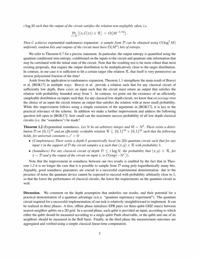
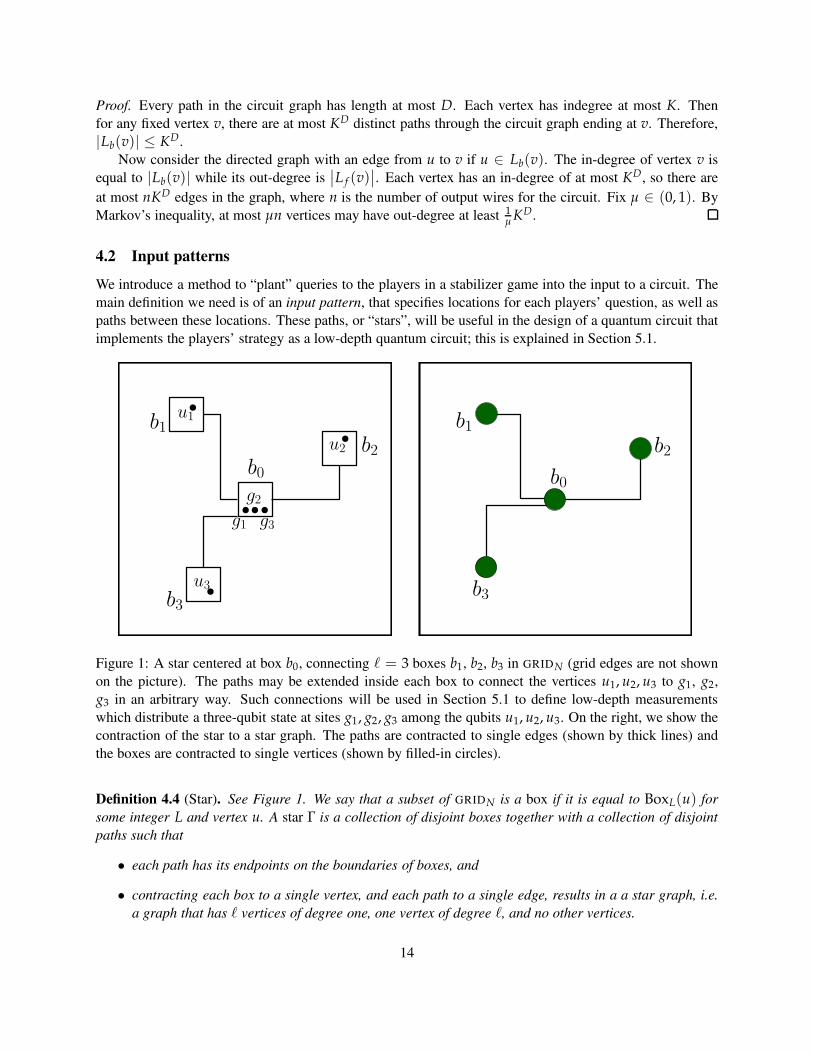
Figure 1: A star centered at box b0, connecting ℓ = 3 boxes b1, b2, b3 in GRIDN (grid edges are not shown

on the picture). The paths may be extended inside each box to connect the vertices u1, u2, u3 to g1, g2,

g3 in an arbitrary way. Such connections will be used in Section 5.1 to define low-depth measurements

which distribute a three-qubit state at sites g1, g2, g3 among the qubits u1, u2, u3. On the right, we show the

contraction of the star to a star graph. The paths are contracted to single edges (shown by thick lines) and

the boxes are contracted to single vertices (shown by filled-in circles).

Definition 4.4 (Star). See Figure 1. We say that a subset of GRIDN is a box if it is equal to BoxL(u) for

some integer L and vertex u. A star Γ is a collection of disjoint boxes together with a collection of disjoint

paths such that

• each path has its endpoints on the boundaries of boxes, and

• contracting each box to a single vertex, and each path to a single edge, results in a a star graph, i.e.

a graph that has ℓ vertices of degree one, one vertex of degree ℓ, and no other vertices.

14

We use the term central box to refer to the unique box which contains one endpoint of every path. If b0 is the

central box, we may say that the star Γ is centered at b0. By abuse of notation, we often write Γ to refer to

the set of vertices contained in the paths and boxes of Γ.

The following definition captures exactly the amount of information that we need to remember about a

given circuit C in order to talk about the spread of correlations within C — we will forget everything about

the circuit except some information about its lightcones.

Definition 4.5 (Input pattern). Let G be an (ℓ, k, m) stabilizer game. Let 1 ≤ r ≤ N be integer. An input

pattern associated with (G, N, r) is a tuple P = (u(i), Γ(i))1≤i≤r such that

• each u(i) = (u(i)1 , . . . , u

(i)ℓ) is an ℓ-tuple of vertices of GRIDN , which we refer to as input locations,

• each Γ(i) is a star,

• the vertices of u(i) are contained in distinct noncentral boxes of Γ(i). For a vertex u, we write Box(u)for the box that contains u.

Definition 4.6 (Circuit specification). A circuit specification S on GRIDN is a triple S = (L f , BADin, BADout)such that for all u ∈ GRIDN , L f (u) ⊆ GRIDN is a set called the forward lightcone associated with u, and

BADin, BADout ⊆ GRIDN are sets called the bad input set and bad output set respectively.

Definition 4.7. For integer B, Rin, Rout we say that a circuit specification S = (L f , BADin, BADout) on

GRIDN is (B, Rin, Rout)-bounded if the following hold: |BADin| ≤ Rin, |BADout| ≤ Rout, and for every

u ∈ GRIDN\BADin it holds that |L f (u)| ≤ B.

Given a fixed circuit specification, the following definition captures the conditions that are required for

an input pattern so that the circuit game associated with that input pattern can be reduced to a nonlocal game

(the reduction is explained in Section 5).

The intuition to keep in mind for the definition is as follows: each player in the nonlocal game receives

her input from one of the input locations and puts her output along the paths of the star. Each player also puts

some outputs inside their box of the star. In order for it to be possible to implement the strategy locally, we

must have the outputs of each player be causally independent of the inputs of the other players. We ensure

this by checking that the forward lightcone of one player’s input misses the locations of the other players’

outputs.

Definition 4.8 (Causality-respecting patterns). Let S = (L f , BADin, BADout) be a circuit specification. Let

P = (u(i), Γ(i))i be an input pattern. We say that a pair (u(i), Γ(i)) is individually-S-causal with respect

to P if the following hold:4

(a) For each k, the forward lightcone of u(i)k misses Γ(i), except possibly near u

(i)k . More precisely,

L f (u(i)k ) ∩ Γ(i) ⊆ Box(u

(i)k ).

(b) For all (u(j), Γ(j)) ∈ P (with j 6= i) and for all k, the forward lightcone of u(j)k misses Γ(i) entirely,

i.e. L f (u(j)k ) ∩ Γ(i) = ∅.

(c) Γ(i) misses BADout, i.e. Γ(i) ∩ BADout = ∅.

4Recall that we identify a star Γ with the union of the vertex sets of its paths and boxes.

15

Furthermore, we say that a pair (u, Γ) is S-valid if the following conditions hold.

(d) Every input location lies outside of BADin, i.e. u(i)k ∩ BADin = ∅ for all k, i.

We say that an input pattern P is S-causal if every (u(i), Γ(i)) ∈ P is individually-S-causal and S-valid

with respect to P ..

Finally, we introduce a distribution on input patterns so that for any circuit specification S that is

(B, Rin, Rout)-bounded for sufficiently small parameters B, Rin, and Rout, a sample from the distribution

gives an S-causal pattern with high probability (see Section 4.3 and Section 4.4).

Definition 4.9 (Random input patterns). Let L, N ≥ 1, ℓ ≥ 1, and 1 ≤ r ≤ N be integer such that

3L√ℓ+ 1 ≤ M = ⌊N/

√r⌋. Divide GRIDN in r disjoint squares S(1), . . . , S(r) of side length M each.5

Partition each square into T = ⌊ M2L+1⌋2 boxes of side length (2L + 1), in an arbitrary way. For each

possible choice of (ℓ+ 1) distinct boxes b0, b1, . . . , bℓ within a square, fix a collection STARS(b0, . . . , bℓ) of

L/ℓ stars such that

• each star has b0 as its central box and b1, . . . , bℓ as its other boxes,

• the total length of the paths in any star is at most 2ℓM, and

• the paths of the distinct stars are vertex-disjoint.

Consider the following distribution D(r)(N, L) on input patterns on GRIDN . For each i ∈ 1, . . . , rselect b

(i)0 , . . . , b

(i)ℓ

uniformly at random among the T boxes that partition the i-th square S(i), for j ∈1, . . . , ℓ, a vertex u

(i)j uniformly at random within the j-th selected box. Finally, select a star Γ(i) ∈

STARS(b(i)0 , b

(i)1 , . . . , b

(i)ℓ) uniformly at random. Return the input pattern P = (u(i), Γ(i))1≤i≤r.

4.3 Single-input patterns

We’d like to show that patterns in the support ofD(r) are “very nearly” S-causal for most S in the sense that

removing only an exponentially small fraction of inputs yields an S-causal pattern. To warm up, we argue

that for any (B, Rin, Rout)-bounded circuit specification S , an input pattern sampled from the distribution

D(1) introduced in Definition 4.9 is S-causal with high probability. We use this single-input analysis later

to show that in a many-input pattern, most of the inputs are individually-S-causal.

In this subsection only, we use M instead of N to denote the grid size. We do this because the distribution

D(r)(N, L) can be (informally) thought of as the direct product of r copies of D(1)(M, L), and the former

is of greater interest to us.

Lemma 4.10. Let M ≥ 1, 1 ≤ B, L ≤ M/4 and 0 ≤ Rin, Rout ≤ M2 be integer. Let S = (L f , BADin, BADout)be a circuit specification for GRIDM that is (B, Rin, Rout)-bounded. Let P = (u, Γ) be drawn from the

distribution D(1) introduced in Definition 4.9. Then the probability that (u, Γ) is not individually-S-causal

with respect toP is O(L2(Rout + B)/M2 +(Rout + B)/L). Moreover, the probability that P is not S-valid

is O(Rin/M2). Overall, the probability that P is not S-causal is at most

O(

L2(Rout + B)/M2 + (Rout + B)/L + Rin/M2)

, (11)

where the O notation hides factors polynomial in ℓ.

5It does not matter where these squares are located, as long as they do not overlap.

16

Proof. We check all conditions in Definition 4.8. Since P contains only one (input, star) pair, condition (b)

(which restricts the interactions between pairs) is satisfied automatically.

Now we check conditions (a) and (c). Call a box bad if it intersects BADout. Under D(1) there are

⌊M/(2L + 1)⌋2 ≥ 1/4(M/2L)2 possible box locations. By a union bound, the probability that any box

is bad is at most 16L2Rout/M2 = O(L2Rout/M2). There are at least L/ℓ possible choices for the paths

of Γ. Since all such choices are disjoint, again by a union bound the probability that Γ ∩ X 6= ∅ for some

subset X is at most ℓ |X| /L. Letting X = BADout ∪⋃

i L f (ui), so that |X| ≤ Rout + ℓB, we see that the

probability of violating condition (a) or condition (c) is at most O(ℓRout+ℓ2B

L

).

Similarly, since the uj are chosen independently, for any u 6= u′ ∈ u0, u1, . . . , uℓ the probability that

L f (u) ∩ Box(u′) 6= ∅ is 16L2B/M2 = O(L2B/M2).

Finally we check condition (d). Any uj is chosen independently among (2L + 1)2 ≥ M2/8 = Ω(M2)possibilities, so the probability that uj ∈ BADin is at most 8Rin/M2 = O(Rin/M2); we conclude by the

union bound, and absorb the parameter ℓ in the O(·).

4.4 Arbitrary-input patterns

We extend the argument from the previous section to the case where the input pattern contains more than

one input.

Lemma 4.11 (Random input patterns are usually causal). Let N ≥ 1, 1 ≤ r ≤ N and 1 ≤ B, Rin, L ≤ N/4be integer. Let S = (L f , BADin, ∅) be a circuit specification for GRIDN that is (B, Rin, 0)-bounded. Then

the probability that an input pattern P chosen according to D(r)(N, L) (as defined in Definition 4.9) is not

S-causal is at most O(r2B(r(L2 + Rin)/N2 + 1/L)).

Proof. Let P = (u(i), Γ(i)) be an input pattern chosen according to D(r)(M, L). For i ∈ 1, . . . , r we

let P (i) be the single-pair pattern (u(i), Γ(i)). Let Xi be the indicator variable that the pair (u(i), Γ(i)) is

not individually-S-causal with respect to P . Let Yi be the indicator that (u(i), Γ(i)) is not S-valid. To see

that P is S-causal, it suffices to check that each input is S-valid and individually-S-causal with respect to

P . This is true if and only if ∑i Xi = 0 and ∑i Yi = 0. We first bound the latter event.

Claim 4.12. It holds that

Pr(

∑j

Yj 6= 0)

= O(r2Rin/N2

). (12)

Proof. Applying the second bound in Lemma 4.10 and using that M = ⌊N/√

r⌋ it follows that for any

i ∈ 1, . . . , r,

Pr (Yi 6= 0) = Pr(P (i) is not S-valid

)≤ 8Rin/M2 = O

(rRin/N2

).

The claim follows by a union bound over the r patterns P (i).

Next we turn to the Xi.

Claim 4.13.

Pr(

∑i

Xi 6= 0)

= O(r2B(rL2/N2 + 1/L)

)+∑

i

Pr(

∑j 6=i

Yj 6= 0)

. (13)

17

Proof. For any i ∈ 1, . . . , r let

BAD(i)out =

⋃

k 6=i

(∪j L f (u

(k)j ))

,

and define a specification S (i) = (L f , BADin, BAD(i)out). With these definitions, it follows that

Pr(Xi = 0) = Pr(P (i) is individually-S-causal

)

≥ Pr(P (i) is individually-S (i)-causal

). (14)

Indeed condition (c) of being individually-S (i) -causal (see Definition 4.8) implies all conditions of being

individually-S-causal for S = (L f , BADin, ∅).

In the event that P (j) is S-valid for all j 6= i (that is, when ∑j 6=i Yj = 0) we know that L f (u(k)j ) ≤ B

for each (j, k) ∈ 1, . . . , ℓ × 1, . . . , r, and thus that |BAD(i)out| ≤ ℓrB = O(rB). Using that the marginal

distribution of a single pair (u(i), Γ(i)) from P is equal to D(1)(M, L) (when seen as a distribution on the

square S(i) associated with (u(i), Γ(i))), it follows from the bound in Lemma 4.10 that for any i ∈ 1, . . . , r,

Pr(

Xi 6= 0∣∣∣∑

j 6=i

Yj = 0)

= O(rB(rL2/N2 + 1/L)

). (15)

Applying the union bound,

Pr(

∑i

Xi 6= 0)≤∑

i

Pr (Xi 6= 0)

≤∑i

Pr(

Xi 6= 0∣∣∣∑

j 6=i

Yj = 0)+ Pr

(∑j 6=i

Yj 6= 0)

≤ O(r2B(rL2/N2 + 1/L)

)+∑

i

Pr(

∑j 6=i

Yj 6= 0)

,

where the last line follows from (15).

To conclude the proof of the lemma we write

Pr(P is not S-causal

)= Pr

(∑

i

Xi + Yi 6= 0)

≤ Pr(

∑i

Xi 6= 0)+ Pr

(∑

j

Yj 6= 0)

≤ O(r2B(rL2/N2 + 1/L)

)+ ∑

i

Pr(

∑j 6=i

Yj 6= 0)+ O

(r2Rin/N2

)

≤ O(r2B(rL2/N2 + 1/L)

)+ O

(r3Rin/N2

)+ O

(r2Rin/N2

)

= O(r2B(r(L2 + Rin)/N2 + 1/L)

),

where the third line uses (13) and (12) and the fourth uses (12).

18

The previous lemma shows that a random input pattern P is S-causal with high probability. In this case

we can define a game from P so that in the game, a shallow circuit with specification S can be simulated by

a set of spacelike-separated players. This simulation is perfect when P is exactly S-causal. More generally,

a weaker simulation argument still applies if a small constant fraction of inputs in P are not S-causal. The

next lemma shows that this condition can be guaranteed to hold with much higher probability, exponentially

close to 1 rather than inverse-polynomially close. This bound will be used in the proof of Theorem 1.2.

Lemma 4.14 (Random input patterns are mostly causal with high probability). Let N ≥ 1, 1 ≤ r ≤ Nand 1 ≤ B, Rin, L ≤ N/4 be integer. Let S = (L f , BADin, ∅) be a circuit specification for GRIDN that is

(B, Rin, 0)-bounded. Consider an input pattern P chosen according to D(r)(N, L). Let

PVAL =(u, Γ) ∈ P|(u, Γ) is S-valid

,

PCAUS =(u, Γ) ∈ P|(u, Γ) is individually-S-causal with respect to PVAL

.

Then there exists universal constants C, C′ > 0 such that if p = C′rB(rL2/N2 + ℓ/L) then for any t > 0,

Pr(|PCAUS| ≥ r(1− p)− 2t

)≥ 1− 2 exp

(−t2/8r

), (16)

Pr(|PVAL| ≥ r(1− CrRin/N2)− t

)≥ 1− 2 exp

(−2t2/r

). (17)

For later convenience we note that (16) and (17) can be combined by a union bound to obtain

Pr(|PVAL ∩ PCAUS| ≥ r(1− CrRin/N2 − 2p)− 3t

)≥ 1− 4 exp

(− t2

8r

). (18)

Proof. The proof relies on concentration arguments to bound the probabilities in (16) and (17). The second

bound, (17), is easier to show, because it can be expressed as a bound on a sum of independent random

variables. The following claim establishes the bound.

Claim 4.15. There is a universal constant C > 0 such that for any t > 0,

Pr(|PVAL| ≥ r(1− CrRin/N2)− t

)≥ 1− 2 exp

(− 2t2

r

).

Proof. For i ∈ 1, . . . , r let Vi be the indicator variable for the event that (u(i), Γ(i)) is S-valid. Since

in D(r)(N, L) the (u(i), Γ(i)) are chosen independently within the disjoint squares S(i), it follows from the

definition of S-valid that the Vi are independent. Using the bound shown in Lemma 4.10 it follows that for

any i ∈ 1, . . . , r,E[Vi] = 1− CRin/M2 , (19)

for some constant C > 0 and where M = ⌊N/√

r⌋. We conclude by applying Hoeffding’s inequality:

Pr(|PVAL| ≤ r(1− CRin/M2)− t

)= Pr

( r

∑i=1

Vi ≤ r(1− CRin/M2)− t)

≤ Pr(1

r

∣∣∣r

∑i=1

Vi −r

∑i=1

E [Vi]∣∣∣ ≥ t/r

)

≤ 2 exp(−2t2/r

).

19

The proof of the remaining bound (16) is made a little delicate by the fact that the condition that a pair

(u, Γ) ∈ P is individually-S-causal is a global condition, so that PCAUS is not directly expressible as a sum

of independent random variables. To get around this, we first make a few definitions.

Let P = (u(i), Γ(i)) be an input pattern chosen at random according to the distribution D(r)(M, L).For i ∈ 1, . . . , r define

BAD<iout =

⋃

k<i s.t.(u(k),Γ(k)) is S-valid

(∪j L f (u

(k)j ))

, BAD>iout =

⋃

k>i s.t.(u(k),Γ(k)) is S-valid

(∪j L f (u

(k)j ))

,

and BAD(i)out = BAD

<iout∪ BAD

>iout. From the assumption that the circuit specification S is (B, Rin, 0)-bounded,

and since BAD(i)out is defined as a union of the lightcones of only the valid pairs (u(k), Γ(k)), it follows that

for all i, |BAD(i)out| ,|BAD

<iout|, |BAD

>iout| are each at most rB.

Recall that in D(r)(M, L) each u(i) is chosen within a square S(i) of side length M = ⌊N/√

r⌋. We

identify S(i) with GRID(i)M , and introduce a single-pair pattern P (i) = (u(i), Γ(i)) that we think of as a

pattern on GRID(i)M . We further define a specification

S (i) = (L f , BADin, BAD(i)out)

on GRID(i)M .

Let Xi be the indicator variable for the event that the pair (u(i), Γ(i)) is not individually-S (i) -causal with

respect to PVAL. The following claim relates the Xi to PCAUS.

Claim 4.16. It holds that |PCAUS| ≥ ∑ri=1 Xi.

Proof. Note that whenever P (i) is individually-S (i) -causal with respect to PVAL, it is also individually-S-

causal with respect to PVAL. This follows by noting that for the given definition of BAD(i)out, condition (c)

of being individually-S (i) -causal with respect to P implies conditions (b) and (c) of being individually-

S-causal with respect to PVAL. Therefore, ∑i Xi is an upper bound on the number of P (i) which are not

individually-S-causal with respect to PVAL.

The previous claim reduces our task to showing a high-probability lower bound on ∑ Xi. The random

variables Xi are dependent. To obtain a bound, we apply a Martingale argument to two related sequences of

random variables, defined as follows. First introduce specifications

S (<i) = (L f , BADin, BAD<iout) and S (>r−i) = (L f , BADin, BAD

>(r−i)out )

on grid GRID(i)M , an let Yi (resp. Zi) as the indicator variable for the event that (u(i), Γ(i)) is not individually-

S (<i)-causal (resp. individually-S (>r−i)-causal) with respect to P (i). The next claim relates Yi and Zr−i to

Xi.

Claim 4.17. For each i ∈ 1, . . . , r, it holds that Xi = Yi ∨ Zr−i.

Proof. The claim follows by noting that, in Definition 4.8, the conditions (a) for Xi, Yi and Zr−i are equiv-

alent. Condition (b) for Xi is equivalent to the event that condition (c) for both Yi and Zr−i is true. Finally,

condition (c) for Xi is vacuous, and conditions (b) for both Yi and Zr−i are vacuous.

The following claim almost finishes the proof.

20

Claim 4.18. There is a universal constant C′ > 0 such that if p = C′rB(rL2/N2 + ℓ/L)) then for any

t > 0,

Pr( r

∑i=1

Yi ≥ t + rp)≤ exp

(−t2

2r

),

Pr( r

∑i=1

Zi ≥ t + rp)≤ exp

(−t2

2r

).

Proof. The proof is based on a Martingale tail bound. For any i ∈ 1, . . . , r, let Y<i = Yk|k < i and

Z>i = Zk|k > i. Note that Yi (resp. Zi) depends only on the underlying circuit C together with the

selection of pairs in squares S(j) for j ≤ i (resp. j ≥ i). It follows from the bound shown in Lemma 4.10

that

E[Yi|Y<i] = O(rB(rL2/N2 + ℓ/L)

), (20)

and similarly

E[Zi|Z>i] = O(rB(rL2/N2 + ℓ/L)

). (21)

Let p denote the maximum of the bounds on the right-hand side of (20) and (21), and assume p ≤ 1. For

any n ∈ 1, . . . , r define Yn = ∑ni=1 Yi − np and Zr−n = ∑

ri=r−n Zi − np. Then

E[Yn|Y<n] = E[Yn − p + Yn−1|Y<n] ≤ Yn−1 ,

and

E[Zr−n|Z>r−n] = E[Zr−n − p + Zr−n+1|Z>r−n] ≤ Zr−(n−1) .

Additionally, it always holds that

|Yn − Yn−1| ≤ |Yn − p| ≤ max(1− p, p) ≤ 1 ,

where the last inequality follows from the assumption that p ≤ 1. Similarly,

|Zr−n − Zr−(n−1)| ≤ |Zr−n − p| ≤ max(1− p, p) ≤ 1 .

Thus, both Yn, and Zr−n form super-martingale sequences for increasing n. Defining Y0 = Zr = 0 and

applying Azuma’s inequality gives

Pr(Yn − Y0 ≥ t) = Pr(Yn ≥ t) ≤ exp

( −t2

2n max(1− p, p)2

)≤ exp

(−t2

2n

),

and

Pr(Zr−n− Zr ≥ t) = Pr(Zr−n ≥ t) ≤ exp

( −t2

2n max(1− p, p)2

)≤ exp

(−t2

2n

).

Setting n = r proves the claim.

Using Claim 4.17 it follows that ∑ri=1 Xi ≤ ∑

ri=1 Yi + ∑

ri=1 Zi. Therefore, for any t > 0

Pr( r

∑i=1

Xi ≥ 2t + 2rp)≤ Pr

( r

∑i=1

Yi + Zi ≥ 2t + 2rp)

≤ Pr( r

∑i=1

Yi ≥ t + rp)+ Pr

( r

∑i=1

Zi ≥ t + rp)

≤ 2 exp

(−t2

2r

),

21

where the last inequality follows from Claim 4.18. Replacing t with t/2 and using Claim 4.16 proves (16).

4.5 Derandomization

Lemma 4.11 states that if a pattern is chosen according to the distribution D(r)(M, L), then it is S-causal

with probability that is close to 1, regardless of the choice of S . The following lemma shows that it is

possible to partially derandomize the distribution, at little loss in the success probability.

Lemma 4.19. Let N ≥ 1 be an integer and η > 0. Let L, B, Rin, r be integer such that

B = O(Nη) , L = O(N4/7+η) , and r = O(N2/7−2η) , (22)

Then using O(log2 N) uniformly random bits it is possible to sample from a distribution D(r) on input

patterns P for GRIDN such that for any circuit specification S that is (B, Rin, 0)-bounded, P is S-causal

with probability 1−O(N−η), and a random (u, Γ) ∈ P is valid with probability O(Rin/N2 + N−η).

Proof. The choice of parameters made in the lemma is such that r3BL2/N2 = O(N−η) and r2B/L =O(N−η), so Lemma 4.11 gives that P sampled according to D(r) is S-causal with probability 1−O(N−η),and a random (u, Γ) ∈ P is valid with probability O(Rin/N2).

A pattern in the support of D(r)(M, L) can be specified using O(r log(N)) uniformly random bits: for

each i ∈ 1, . . . , r, there are O(log N) random bits to specify the locations of the u(i)j , and O(log N)

additional bits to specify the star that connects the u(i)j . Given any choice of such random bits, and a

fixed circuit specification, by Savitch’s theorem it is possible to decide whether the pattern is S-causal in

O(log2 N) space, given read-only access to the circuit graph determining S . This allows us to apply the

INW pseudorandom generator for small-space circuits [INW94] with O(log2 N) seed to obtain the claimed

result, with the additional error O(N−η) being due to the pseudorandom generator.

5 Circuit games

Let N ≥ 1 be an integer grid size. Let r ≥ 1 be an integer number of repetitions. Let G be an (ℓ, k, m)stabilizer game. In this section we design a circuit game G = GG,N,r associated with (G, N, r) in a way

that the circuit game has similar completeness and soundness properties as G (more precisely, as a rotated,

stretched game obtained from G, using the stars in an input pattern P associated with (G, N, r) that is

provided as input to the circuit to define the length of the stretches; see Section 3.2 for the definition of

rotated and stretched games).

We first give a general definition that specifies what we mean by a “circuit game”.

Definition 5.1 (Circuit game). Given input and output sets I , O respectively, a circuit game is a relation

R ⊆ I ×O, together with a probability distribution π on I . We say that a circuit C wins the circuit game

(R, π) with probability p if, on average over an input x ∈ I sampled according to π, the circuit returns an

output y ∈ O such that (x, y) ∈ R with probability p.

To specify the relation associated with the circuit game we will construct from G it is convenient to

first introduce a quantum circuit that succeeds in the game with certainty. This is done in Section 5.1. In

Section 5.2 we give the definition of the circuit game.

22

5.1 Definition and completeness

Informally, the game GG,N,r is obtained by “planting r copies of G in the grid GRIDN”. Let P be an input

pattern associated with (G, N, r) (see Definition 4.5). Let k = maxj kj be the maximum number of qudits

used by a player in the honest strategy for G, |ψ〉 the (kℓ)-qubit state used in the strategy (padded if needed),

and D the depth of a circuit that prepares |ψ〉 from |0〉. Assume that D ≥ 2. We describe a depth (D + 1)quantum circuit Cideal that takes an input from

I =P : input pattern for G

×(x

(i)1 , . . . , x

(i)ℓ)1≤i≤r : r-tuple of queries in G

, (23)

and returns a string in the output set

O =r

∏i=1

ℓ

∏j=1

((Z2k

d )Γ(i)j × (Z

m j

d )u(i)j

). (24)

In (24) we have used the vertices in Γ(i)j and the u

(i)j to label indices of the elements of O. Note that these

are always distinct. In Section 5.1.2 we show how to modify the format for the input and the output in a way

that the circuit can be made geometrically local on a 2D grid.

The computation performed by the circuit Cideal proceeds in three stages:

• In the first stage, the circuit initializes a lattice of qudits as follows. Each vertex in GRIDN is associated

with 4k qudits, organized in 4 groups of k that we call the “left”, “right”, “top” and “bottom” groups

associated with that vertex. Each of these groups is initialized in a maximally entangled state with

the group from the neighboring grid vertex that is closest to it, i.e. the “top” group at vertex (i, j) is

associated with the “bottom” group at vertex (i, j + 1), etc. In addition, for each center location g(i)

of a star Γ(i) in P , the circuit creates the state |ψ〉 on the (kℓ) qudits associated with the ℓ vertices

(g(i)1 , . . . , g

(i)ℓ); for each vertex g

(i)j , a group of qudits is used that is not connected to the next vertex

in the path Γ(i)j . (This replaces the creation of the maximally entangled state, for that group of qudits.)

This step can be implemented in depth max(2, D).

• In the second stage, the circuit implements an entanglement transfer protocol as described in Sec-

tion 5.1.1, using each of the ℓ simple paths that form a star Γ(i) from P to route the qudits of |ψ〉. The

measurement outcomes in (Zd)2k from the teleportation measurements obtained at each vertex in Γ(i)

are recorded at the location at which they are obtained, and will eventually form part of the output of

the circuit. This step can be completed in depth 1.

• In the last stage, the circuit implements the honest quantum strategy for the game G, using locations

u(i)j indicated in P to specify the k qudits to be used by the j-th player (the group used is the one

closest to the endpoint of the path Γ(i)j ), and x

(i)j as the player’s question. The outcomes obtained are

returned as part of the output. This step can be completed in depth 1, and can be executed in parallel

with the previous step.

The following lemma states that outputs generated by this circuit satisfy the win condition for an asso-

ciated rotated, stretched game.

Lemma 5.2. Let G be an (ℓ, k, m) stabilizer game, 1 ≤ r ≤ N, and P an input pattern associated

with (G, N, r). Let x(1), . . . , x(r) be an arbitrary tuple of r queries for G. For all i ∈ 1, . . . , r and

23

j ∈ 1, . . . , ℓ let (r(i)j , a

(i)j ) ∈ (Z2k

d )Γ(i)j ×Z

m j

d be the outputs generated by an execution of Cideal on input

P and (x(1), . . . , x(r)). Then for any i ∈ 1, . . . , r, (r(i)j , a(i)j )j∈1,...,ℓ is a valid ℓ-tuple of answers for

the players in the rotated stretched game GS,R

Γ(i) , on query x(i).

Proof. The lemma follows from the definition of Cideal, the properties of the entanglement transfer protocol

stated in Lemma 5.5, and the definition of the rotated, stretched game.

5.1.1 Entanglement transfer

We introduce a simple procedure for routing entanglement along a path, such that nearest neighbors on the

path have been initialized in a maximally entangled state. This is a standard calculation; for completeness

we include the details.

Lemma 5.3 (Entanglement transfer I). Let d ≥ 2 and |EPRd〉 = 1√d

∑i |ii〉 a maximally entangled state on

d-dimensional qudits. Let a, b ∈ Zd and

|ψ〉ABCD

=(Xa

A ⊗ ZbB |EPRd〉AB

)⊗ |EPRd〉CD

a maximally entangled state on four qudits. Then upon measuring the qudits in registers B and C in the Bell

basis Xx ⊗ Zy |EPRd〉 : x, y ≤ d, the post-measurement state is equal (up to global phase) to

(Xa+x

A⊗ Z

b−yD|EPRd〉

)AD⊗(Xx

B ⊗ ZyC|EPRd〉

)BC

. (25)

Proof. We evaluate the post-measurement state by computing the result of applying the measurement pro-

jector onto the state Xx ⊗ Zy |EPRd〉. Let ω = e2πi/d.(Xx ⊗ Zy |EPRd〉〈EPRd|BC X−x ⊗ Z−y

)Xa

A ⊗ ZbB |EPRd〉AB ⊗ |EPRd〉CD

= XxB ⊗ Z

yC

(1

d ∑k,l

|kk〉〈ll|)

X−xB ⊗ Z

−yC Xa

A ⊗ ZbB

1

d ∑i,j

|i〉 |i〉 |j〉 |j〉

= XxB ⊗ Z

yC

(1

d ∑k,l

|kk〉〈ll|)

X−xB ⊗ Z

−yC

1

d ∑i,j

ωbi |i + a〉 |i〉 |j〉 |j〉

= XxB ⊗ Z

yC

(1

d ∑k,l

|kk〉〈ll|)

1

d ∑i,j

ωbi−yj |i + a〉 |i− x〉 |j〉 |j〉

= XxB ⊗ Z

yC

1

d2 ∑i,j,k

ωbi−yjδi−x,j |i + a〉 |k〉 |k〉 |j〉

= XxB ⊗ Z

yC

1

d2 ∑j,k

ωb(j+x)−yj |j + x + a〉 |k〉 |k〉 |j〉

= ωbxXa+xA ⊗ Z

b−yD |EPRd〉AD ⊗ Xx

B ⊗ ZyC |EPRd〉BC .

Lemma 5.4 (Entanglement transfer II). Let n ≥ 1, and L1, . . . , Ln, R1, . . . , Rn qudit registers such that each

Li is maximally entangled with Ri. Suppose one performs (n− 1) Bell basis measurements on qudit pairs

(R1, L2), . . . , (Rn−1, Ln), so that the post measurement state of the i-th pair is Xxi ⊗ Zyi |EPRd〉. Let x =

∑i xi and z = ∑i zi. Then the post measurement state of the remaining pair (L1, Rn) is Xx ⊗ Z−z |EPRd〉.

24

Proof. The (n − 1) Bell basis measurements commute, so we can think of them as being performed in

sequence, performing the measurement on (Rk, Lk+1) at the k-th step. Using Lemma 5.3 and induction, one

can check that after the k-th measurement, the qudits (L1, Rk+1) are in post-measurement state X∑ki=1 xi ⊗

Z−∑ki=1 zi |EPRd〉.

Lemma 5.5 (Low-depth state teleportation). Let k ≥ 1 be an integer and |ψ〉 a k-qudit state that is locally

maximally mixed in the sense that the marginal density matrix at any one qudit is the maximally mixed state.

Let N ≥ 1 and A and B be ordered lists of vertices in GRIDN with |A| = |B| = k. Let

Γj

1≤j≤k

be a

set of k vertex-disjoint, even-length paths on the grid, each with one endpoint in A and one endpoint in B.

For any i ∈ 1, . . . , k denote the points of Γi as v0 · · · vl with endpoints v0 ∈ A, vl ∈ B. To each of the

“odd-even” qudit pairs (v1, v2), (v3, v4), . . . , (vl−1, vl) apply a gate taking the two qudit state to |EPRd〉.Next, measure each of the “even-odd” qudit pairs (v0, v1), (v2, v3), . . . , (vl−2, vl−1) in the Bell basis. Let

Xai

j ⊗ Zbi

j |EPRd〉 be the post-measurement state of the j-th pair.

Let P be the weight k Pauli operator supported on the qudits of B such that the i-th qudit of P acts as

XaiZ−bi

. Then the post-measurement state of the qudits in B is P |ψ〉.

Proof. We analyze the circuit one path at a time. Fix i ∈ 1, . . . , k. Let xi ∈ A be one endpoint of Pi and

yi the other. Suppose that |φ〉 is any locally maximally mixed state on a set C of qubits with xi ∈ C. Let

C′ = C \ xi. Then there is a unitary V : C′ → C′1⊗ C′2 such that

I ⊗V |φ〉xiC= |EPRd〉xiC

′1⊗ |φ′〉C′2 . (26)

Now suppose we apply V and then apply the entangling gates and measurements along Γi. By Lemma 5.4,

the state of qudits yi and C′1 is

Xai ⊗ Z−bi |EPRd〉yiC′1= Xai

Z−bi ⊗ I |EPRd〉yiC′1

. (27)

The equality in (27) can be verified by noticing that Z⊗ Z† stabilizes |EPRd〉. Applying V† gives

(I ⊗V†)(XaiZ−bi ⊗ I) |EPRd〉yiC

′1⊗ |φ′〉C′2 = (Xai

Z−bi ⊗ I) |φ〉yiC′. (28)

Notice that the operation along the path commutes with V. Therefore, applying V, applying that operation,

and then applying V† is equivalent to just applying that operation.

Notice that the resulting state continues to be locally maximally mixed. Therefore, we can apply the

above repeatedly until all of the path circuits have been applied. Then the final state is as desired.

5.1.2 Geometric locality

We explain how to modify the input and outputs sets I andO specified in (23) and (24) respectively in a way

that both input and output are Boolean strings of the same length that can be organized in a 2-dimensional

pattern and such that the circuit described in Section 5.1 can be implemented in the same depth (D + 1)using only geometrically local gates.

Recall that the input to the circuit consists of an input pattern P = (Γ(i), u(i))1≤i≤r together with an

r-tuple of queries (x(i)1 , . . . , x

(i)ℓ)1≤i≤r in G. Recall also that we think of the circuit as being organized on

an N × N grid of vertices, such that each vertex contains 4 groups of k qudits, each group facing one of the

vertex’ nearest neighbors on the grid. We index the input and output sets by grid vertices, with each vertex

associated with an element taken from a constant-size alphabet Σ that is defined in (29) below.

25

Each star Γ(i) specifies ℓ paths Γ(i)j from the central box to the noncentral boxes. Assign to one point

in each noncentral box the label u(i)j . Also assign to ℓ points inside the central box the labels g

(i)j . Extend

the paths Γ(i)j so that their endpoints are u

(i)j and g

(i)j . We naturally distribute each question x

(i)j at the grid

vertex indicated by u(i)j .

For each edge (v, w) in the path, at vertex v (resp. w) we include a symbol that indicates that a telepor-

tation measurement is to be performed between the group of k qudits nearest to vertex w (resp. v). For any

grid vertex v, the output of the circuit at vertex v is either an answer in G, a(i)j ∈ (Zd)

m j , or a teleportation

measurement outcome, which is an element of (Zd)2k. A question x

(i)j is an element of (Zk

d)m j . This leads

us to a circuit specification that considers the input and output sets

I = O = ΣGRIDN , where Σ = 0, 12mk⌈log d⌉ , (29)

where m = maxj mj and we fixed an arbitrary embedding of the natural input and output alphabets in Σ.

Note that not all input strings are used; since we consider the parameters d, m, k to be constants (depending

only on the type of stabilizer game chosen), the cardinality of the alphabet Σ is constant.

5.2 Circuit game definition

Having specified the ideal (or, “honest”) quantum circuit that we have in mind, we are ready to give a formal

definition of the circuit game associated with r copies of a stabilizer game G. Recall the definition of the

distribution D(r) on input patterns given in Definition 4.9. (For clarity, we omit the arguments N, L, for

which we will eventually make an appropriate choice.)

Definition 5.6. Let G be an (ℓ, k, m) stabilizer game and 1 ≤ r ≤ N integer. The circuit game GG,N,r is

a game on the input and output sets defined in (29). The input distribution π is obtained by independently

sampling an input pattern P according to D(r) and a tuple of r independent queries (x(1), . . . , x(r)) for G,

and encoding them as an element of I as described in Section 5.1.2. The relation R ⊆ I ×O is defined as

the support of the output distribution of the circuit described in Section 5.1, when it is provided an input in

the support of π.

Skipping ahead, we note that in Section 6.2 we consider a slight variation of the circuit game GG,N,r

from Definition 5.6, where the r query tuples to G are no longer independent and the win condition is

relaxed to allow failure in some of the game instances. These modifications allow us to obtain a circuit

game whose inputs can be sampled using few random bits (polylogarithmic in N), and that can be won with

high probability by a circuit whose gates are subject to a limited amount of noise.

5.3 Soundness

We describe a reduction from circuit strategies (i.e. circuits with constant fan-in and bounded depth) in the

circuit game introduced in Definition 5.6 to strategies for the players in the game G. The next lemma refers

to the notions of lightcone, input pattern, and circuit specification introduced in Section 4.1 and Section 4.2,

and of rotated, stretched and repeated game introduced in Section 3.2 and Section 3.3.

Lemma 5.7 (Circuit locality implies local simulation). Let G = GG,N,r be a circuit game as in Defini-

tion 5.6. Let P = (u(i), Γ(i))1≤i≤r be an input pattern in the support of the input distribution for G.

26

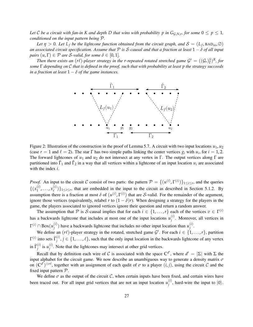
Let C be a circuit with fan-in K and depth D that wins with probability p in GG,N,r, for some 0 ≤ p ≤ 1,

conditioned on the input pattern being P .

Let η > 0. Let L f be the lightcone function obtained from the circuit graph, and S = (L f , BADin, ∅)an associated circuit specification. Assume that P is S-causal and that a fraction at least 1− δ of all input

pairs (u, Γ) ∈ P are S-valid, for some δ ∈ [0, 1].Then there exists an (rℓ)-player strategy in the r-repeated rotated stretched game G ′ = ((Gr)S

Γ)R, for

some Γ depending on C that is defined in the proof, such that with probability at least p the strategy succeeds

in a fraction at least 1− δ of the game instances.

Γ1 Γ2

u1 g1 g2 u2

Lf(u1) Lf(u2)

~Γ1~Γ2

Figure 2: Illustration of the construction in the proof of Lemma 5.7. A circuit with two input locations u1, u2

(case r = 1 and ℓ = 2). The star Γ has two simple paths linking the center vertices gi with ui, for i = 1, 2.

The forward lightcones of u1 and u2 do not intersect at any vertex in Γ. The output vertices along Γ are

partitioned into Γ1 and Γ2 in a way that all vertices within a lightcone of an input location ui are associated

with the index i.

Proof. An input to the circuit C consist of two parts: the pattern P = (u(i), Γ(i))1≤i≤r, and the queries

(x(i)1 , . . . , x

(i)ℓ)1≤i≤r, that are embedded in the input to the circuit as described in Section 5.1.2. By

assumption there is a fraction at most δ of (u(i), Γ(i)) that are S-valid. For the remainder of the argument,

ignore those vertices (equivalently, relabel r to (1− δ)r). When designing a strategy for the players in the

game, the players associated to ignored vertices ignore their question and return a random answer.

The assumption that P is S-causal implies that for each i ∈ 1, . . . , r each of the vertices v ∈ Γ(i)

has a backwards lightcone that includes at most one of the input locations u(i)j . Moreover, all vertices in

Γ(i) ∩ Box(u(i)j ) have a backwards lightcone that includes no other input location than u

(i)j .

We define an (rℓ)-player strategy in the rotated, stretched game G ′. For each i ∈ 1, . . . , r, partition

Γ(i) into sets Γ(i)j , j ∈ 1, . . . , ℓ, such that the only input location in the backwards lightcone of any vertex

in Γ(i)j is u

(i)j . Note that the lightcones may intersect at other grid vertices.

Recall that by definition each wire of C is associated with the space Cd′ , where d′ = |Σ| with Σ the

input alphabet for the circuit game. We now describe an unambiguous way to generate a density matrix σ

on (Cd′)⊗rℓ, together with an assignment of each qudit of σ to a player (i, j), using the circuit C and the

fixed input pattern P .

We define σ as the output of the circuit C, when certain inputs have been fixed, and certain wires have

been traced out. For all input grid vertices that are not an input location u(i)j , hard-wire the input to |0〉.

27

Execute the circuit until a vertex v of the circuit graph that is in the forward lightcone of an input vertex

associated with location u(i)j has to be considered. Since no input has been hard-wired for that vertex, the

circuit cannot proceed. There are two cases:

• If the forward lightcone of v intersects the forward lightcone of two different input locations u(i)j ,

then no vertex in the forward lightcone of that location can be on any of the stars Γ(i′) for i′ 6= i (as

otherwise the vertex would be a vertex of Γ whose backwards lightcone contains two distinct input

locations). In that case, trace out the vertex.

• In all other cases, vertex v is in the forward lightcone of a single input location u(i)j . In this case, give

the circuit wire associated with that vertex (in the state that it currently is) to player (i, j).

Finally, split the unassigned vertices on any path Γ(i)j in an arbitrary way among the players; the set Γ

(i)j is

defined as the set of vertices from the star Γ(i) assigned to the j-th player. All remaining unassigned vertices

are traced out.

This procedures specifies the state σ shared by the players (see Figure 2 for an illustration). It remains

to define their observables. Once the game starts, each player uses its input x(i)j in location u

(i)j (encoded

as an input to the circuit game, as specified in Section 5.1.2), and proceeds to complete the execution of the

circuit on the qudits that it holds. If a gate has an output wire that points to a qudit that is not in the player’s

possession, the player measures the qudit and ignores the outcome. Finally, the player measures all qudits

in the locations Γ(i)j in the computational basis, and returns them as its answer (decoded as an answer in G,

as specified in Section 5.1.2).

The fact that this strategy for the players has the same success probability in G ′ as the circuit C in the

circuit game GG,N,r follows from the fact that the success criterion in GG,N,r only involves output vertices

that are along the stars Γ(i), and it can be verified that the joint operations performed by the players in the

above-defined strategy correctly compute the reduced density matrix computed by the circuit on all those

output vertices. Finally, using Lemma 5.5 it can be verified that the success criterion in the circuit game

matches the win condition for the rotated stretched game.

Remark 5.8. The proof of Lemma 5.7 establishes a stronger statement than claimed in the lemma, that will

be useful later. Specifically, the reduction from a circuit to a strategy for the players in G ′ constructed in

the proof applies whenever the input pattern P chosen in the circuit game is S-causal for S the circuit

specification derived from C. Moreover, whenever this is the case the reduction yields a strategy for the

players that exactly reproduces the (suitably decoded) output distribution of the circuit, on any choice of

queries x(i).

We end this section with the proof of Theorem 1.2, that specifies a circuit game for which there is a very

large separation between the optimal winning probabilities of classical low-depth and quantum circuits.

Theorem 1.2 (Exponential Soundness, restated). Let N ≥ 1 be an integer. There exists a circuit game GN

such that the input and output sets are GRIDN ′ for some N′ = O(N), and such that the following hold:

• (Completeness) There exists a depth-4 quantum circuit that succeeds at GN with probability 1.

• (Soundness) For any η < 1/7 there is a constant c > 0 depending on η only such that any classical

circuit of depth D ≤ c log N has success probability at most exp(−Ω(Nη)) in the game.

28

Proof. Let GN = GG,N,r be the circuit game introduced in Definition 5.6, where the stabilizer game G is

instantiated as the GHZ game from Definition 3.14, and let π and P be the input distribution and input

pattern introduced in Definition 5.6 respectively.

Completeness: By Lemma 5.2 the circuit Cideal, as defined from the game GN at the beginning of Section

5.1, wins the game GN with probability at least (ω∗(G))r, where ω∗(G) is the optimal entangled winning

probability for the stabilizer game G. Since ω∗(G) = 1 it follows that Cideal succeeds at GN with probability

1. As noted after Definition 3.14, the shared state |ψ〉GHZ in the optimal strategy for the GHZ game can be

prepared starting from |000〉 by a circuit of depth 3. It follows by definition that Cideal has depth at most 4.

This establishes the completeness part of the corollary.

Soundness: Fix an η ∈ (0, 17). Let C be a classical circuit with fan-in K and depth D ≤ c log N (for c a

sufficiently small constant depending on η) that wins with probability pwin in GG,N,r. We show that if pwin

is too large, then there is a good classical strategy for the players in the game GHZ⌊r/2⌋, the ⌊r/2⌋-repeated

GHZ game defined in Definition 3.10. For an input pattern P in the support of D(r), say that P has a large

S-causal subpattern if there exists a subpattern P ′ ⊆ P such that P ′ is S-causal and |P ′| ≥ ⌊r/2⌋. Define

q as

q = 1− Pr (P has a large S-causal subpattern) . (30)

We first show an upper bound on q. For any pattern P let Pcore = PVAL ∩ PCAUS, where as in

Lemma 4.14,

PVAL =(u, Γ) ∈ P|(u, Γ) is S-valid

,

PCAUS =(u, Γ) ∈ P|(u, Γ) is individually-S-causal with respect to PVAL

.

By construction Pcore is S-causal. To prove an upper bound on q it suffices to place a lower bound on the

probability that |Pcore| ≥ ⌊r/2⌋. Recall that the classical circuit C has fan-in K, depth D ≤ c log N, and

circuit specification S = (L f , BADin, ∅). By Lemma 4.3, we may choose c as a function of η such that S is

(B, Rin, 0)-bounded, where B = O(Nη) and Rin = O(N2−η). By (18) we get

Pr(|Pcore| ≥ r(1− CrRin/N2 − 2p− 3t/r)

)≥ 1− 4 exp

(−t2/8r

), (31)

where p = C′rB(rL2/N2 + ℓ/L). Here ℓ = 3, and the other parameters depend on N. To set parameters,

first recall that B = O(Nη) and Rin = O(N2−η). Set t = r/10, r = Θ(Nη), and L such that L =O(N1−3η) and L = Ω(N4η), which is possible as long as η < 1/7. Then p = O(1) and rRin/N2 = O(1).By choosing the constants appropriately, we can ensure that

1− CrRin/N2 − 2p− 3t/r > 1/2.

With this choice of parameters, (31) implies that |Pcore| ≥ r/2 with probability at least 1− 4 exp (−C′′r),for some constant C′′ > 0. To conclude, note that whenever P contains a S-causal subpattern P ′ ⊆ P such

that |P ′| ≥ r/2 it follows from Lemma 5.7 and Remark 5.8 that the circuit C implies a strategy for (rℓ/2)classical players in the repeated game GHZ⌊r/2⌋. Using that the maximum success probability of classical

players in GHZ is 3/4 and that the classical value multiplies under repetition (since the players are distinct)

it follows that the implied strategy has success probability at most (3/4)⌊r/2⌋.

6 Randomness generation

In this section we give the construction of a circuit game such that any low-depth circuit that succeeds in the

game with non-negligible probability must generate outputs that have large min-entropy, even conditioned

on the inputs and side information that may be correlated with the initial state of the circuit.

29

The main idea for the construction is to embed a large number of copies of a simple stabilizer game Gin a circuit game, as described in Section 5. (We use the Mermin 3-player GHZ game [Mer90a], though

a similar reduction could be performed starting from any stabilizer game whose quantum value is larger

than its classical value.) Using the reduction from Lemma 5.7, it follows from Remark 5.8 that the output

distribution of any circuit that wins with non-negligible probability in the circuit game can be deterministi-

cally mapped to a (stretched, rotated) variant of the r-fold parallel repetition, with r independent groups of

players, of G. This reduction implies that, to bound the output entropy of the circuit, it suffices to place a

lower bound on the output entropy of any strategy in the parallel repeated game.

To accomplish this last step we employ the framework based on the Entropy Accumulation Theorem

(EAT) [DFR16] introduced in [AFDF+18], including the improvements from [DF18]. This framework

allows to place a linear (in the number of repetitions) lower bound on the amount of min-entropy generated

in the sequential repetition of a nonlocal game, using a lower bound on the function that measures the von

Neumann entropy generated in a single instantiation of the game as a function of the success probability.

Our setting of parallel repetition is more constrained (thus in principle easier to analyze) than the sequential

setting, but the results from [AFDF+18, DF18] still give the best rates for both settings.

In Section 6.1 we start by establishing a bound on the single-round randomness for the three-player GHZ

game that takes the form required to apply the framework from [AFDF+18]. In Section 6.2 we combine this

bound with the reduction from circuit games to nonlocal games shown in Section 5 to deduce a family of

randomness-generating circuit games.

6.1 Randomness generation from the GHZ game

We briefly recall the formalism from [AFDF+18], when tailored to our setting (in particular, we focus

on processes specified by quantum strategies in a nonlocal game, instead of arbitrary quantum channels

in [AFDF+18]). The main definition that is needed is that of a min-tradeoff function, which specifies a

lower bound on the amount of randomness generated in a single execution of a nonlocal game, as a function

of the players’ probability of winning in the game. We give the definition for stabilizer games, as introduced

in Definition 3.1.

Definition 6.1 (min-tradeoff function). Let G be an (ℓ, k, m) stabilizer game. Fix a set of measurements

Mxj for the ℓ players in the game. For any ω ∈ [0, 1], let Σ(ω) denote the set of states ρP1···PkR such that

when the players’ state is initialized to ρ (with player i being given register Pi), the players’ strategy wins

the game with probability ω.6

Then a real affine function f on [0, 1] is called an (affine) min-tradeoff function for G and Mxj if it

satisfies

f (ω) ≤ minρ∈Σ(ω)

H(A|QR)M(ρ) ,

where the entropy is evaluated on the post-measurement stateM(ρ) obtained after application of the play-

ers’ measurements, and Q and A are random variables that represent inputs (distributed according to π)

and outputs for the players in G. If f is a min-tradeoff function for a game G and every possible set of

measurements Mxj for the players, then we simply say that f is a min-tradeoff function for G.

To illustrate the definition we apply results from [WBA18] to give a min-tradeoff function for the Mer-

min GHZ game introduced in Definition 3.14. It is well-known (and easily verified) that the best classical

6We may without loss of generality assume that the dimension of R is no more than the sum of the dimensions of the players’

private registers Pj, themselves fixed by the measurements Mxj. Therefore, the set Σ(ω) can be taken to be a compact set.

30

strategy for this game succeeds with probability 34 . This in particular implies that any strategy that wins

with probability strictly larger than 34 cannot be deterministic, hence generates randomness. The following

bound shown in [WBA18] provides a tight lower bound on the conditional entropy present in the outputs of

any strategy that succeeds with sufficiently large probability.7

Lemma 6.2 ([WBA18]). Let τ = (ρ, Mxj) be a strategy with success probability ω ≥ 7

8 in the game

GHZ, where ρ is a density matrix on the provers’ registers P1 · · ·Pℓ and an arbitrary auxiliary register R.

Then

H(

A1A2|RQ)≥ fGHZ(ω) = − log

(5

4− ω +

√3

√(ω − 1

2

)(1−ω

)), (32)

where Q is a random variable that denotes the query to the players, and A1, A2 are random variables that

denote the answers a1, a2 ∈ Z2 from the first two players.

Note that for ω = 1, the bound (32) gives 2 bits of entropy, which is clearly optimal. If ω = 1− ε for

small ε, the bound degrades as 2−O(√

ε).Following the framework from [AFDF+18], the bound provided in Lemma 6.2 already implies a linear

lower bound on the entropy generated by the sequential repetition of the GHZ game. For our purposes it

will be convenient to have a bound on the entropy generated by the stretched, rotated variant of the GHZ

game, as introduced in Section 3.2.

Corollary 6.3 (min-tradeoff function for GHZ). Let 78 < ps < 1. Let Γ be a tuple of sets as in Definition 3.9.

Then the function gps : [0, 1] → R defined by

gps(q) = fGHZ(ps) + (q− ps)d fGHZ

dω(ps)

is a min-tradeoff function for the rotated stretched game GHZS,RΓ .

Proof. First we observe that the bound (32) from Lemma 6.2 applies equally to the the rotated stretched

game GHZS,RΓ , for any fixed Γ. Indeed, fix a strategy (ρ, Mxj

) in GHZS,RΓ . Using Lemma 3.8 we obtain

a strategy τ′ = (ρ, M′xj) for GHZ that has the same success probability. Furthermore, in the coarse-

graining of the strategy the answers A1, A2, A3 ∈ Z2 in τ′ are a deterministic function of the answers

A1, A2, A3 ∈ Z2 × (Z22)|Γ1| in GHZS,R

Γ , where the second factor is for the stretched rotation string. There-

fore the same bound on randomness generation that applies to GHZ applies to GHZS,RΓ (as long as all

outputs in the game are included, which is the case for the definition of a min-tradeoff function).

To conclude, note that the right-hand side of (32) is a convex function of ω, hence it is at least its tangent

at any point.

Recall that our goal is to generate a large amount of randomness by requiring a circuit to play multiple

copies of the game GHZ in parallel. Towards this, we introduce a partially derandomized variant of the

repeated game, where the inputs are chosen according to a very biased distribution in order to save on

the randomness required to generate them. The resulting game is a direct analogue of the protocol for

randomness expansion from the CHSH game given in [DF18].

7See (18) in [WBA18]. The authors prove a stronger bound, that applies to the min-entropy and extends to all success probabil-

ities in the range [3/4, 1]. We only state the weaker bound that will be sufficient for us. To see how the bound stated in Lemma 6.2

is obtained from (18) in [WBA18], use the replacement ω = 12 + M

8 .

31

Definition 6.4. Let r ≥ 1 be an integer. Let p, γ ∈ [0, 1]. Let Γ be a tuple of sets as in Definition 3.9. Let

GHZS,Rr,Γ,p,γ denote the r-fold repetition, as in Definition 3.10, of the rotated, stretched game GHZ with the

following two modifications:

• The r queries, instead of being sampled independently, are chosen according to the following distri-

bution: first, select a subset S ⊆ 1, . . . , r by including each element independently with probability

p; second, select queries x(1), . . . , x(r) ∈ X such that x(i) is sampled as in GHZ when i ∈ S, and

x(i) ← x for i /∈ S, where x is an arbitrary, but fixed, query in GHZ;

• It is only required that the win condition is satisfied for a fraction at least (1− γ) of the tuples of

answers a(i) such that i ∈ S (there is no requirement for i /∈ S).

Corollary 6.3 shows that any sufficiently successful strategy in the (rotated, stretched) game GHZ must

generate outputs that contain a constant amount of entropy. It is therefore natural to expect that a strategy

for the repeated game from Definition 6.4 should generate a linear (in the number of repetitions) amount

of entropy. The difficulty is to obtain a bound on the entropy generated, conditioned on having produced

outputs that satisfy the win condition of the game, but without placing an implicit assumption on the intrin-

sic winning probability of the strategy (which would be difficult to estimate). Moreover, the fact that the

strategy involves all players simultaneously measuring parts of the same entangled state introduces corre-

lations that prevent a direct treatment using techniques appropriate for the simpler case of i.i.d. (identically

and independently distributed) outputs.

The Entropy Accumulation Theorem, as applied in [AFDF+18], is designed specifically to address these

difficulties, and indeed guarantees that the repeated game introduced in Definition 6.4 generates a linear

amount of min-entropy. Here we use the improved results from [DF18],8 that give good bounds even when

the “test probability” p from Definition 6.4 can be very small.

Lemma 6.5. Let r ≥ 1, p, γ ∈ [0, 1], and ε > 0. Let (ρ, Mxj), where ρ is a density matrix on the player’s

private registers together with an ancilla register E, be a strategy for the (3r) players in GHZS,Rr,Γ,p,γ that

succeeds with probability at least ε. Let Q = (Q(1), . . . , Q(r)) (resp. A = (A(1), . . . , A(r))) be random

variables associated with the players’ answers in each copy of GHZ; note that each Q(i) (resp. A(i)) is

itself a 3-tuple. Let ρsAQE

denote the state of AQE conditioned on the players succeeding in the game (the

players’ private registers are traced out). Then

Hεmin(A|QE)ρs ≥ fGHZ(1− γ)r−O

( r√p

(ln

1

εTr(ρs)

)1/2). (33)

Note that the lower bound provided in (33) is non-trivial as soon as p = Ω(log N/r) and ε is at least

inverse-polynomially large (smaller ε is also possible, but requires a larger p).

Proof. The proof is identical to the proof of [DF18, Theorem 6.1], that applies to the CHSH game. The only

change needed is to use the min-tradeoff function from Corollary 6.3 instead of the min-tradeoff function

g∗ for the CHSH game used in [DF18]. The bound (33) follows from the bound stated in [DF18, Theorem

6.1] by noting thatd fdω (1− γ) is bounded by a universal constant.

8The results in [AFDF+18, DF18] apply to a much more general scenario, and in particular allow one to prove bounds on the

entropy generated by an arbitrary sequential process, as long as it satisfies a certain Markov condition. Our setting, which considers

parallel repetition, is easier, and trivially satisfies the required Markov condition.

32

6.2 Randomness generation from low-depth circuits

Using the technique to embed a stabilizer game into a circuit game described in Section 5 we can leverage

the randomness generation results from the previous section to obtain a family of circuit games for certified

randomness expansion. First we define the circuit games that we consider by introducing a randomness-

efficient, noise-tolerant modification of the game from Definition 5.6. Even though we will eventually

instantiate the definition with G = GHZ, we give the definition for a general stabilizer game.

Definition 6.6. Let G be an (ℓ, k, m) stabilizer game and N ≥ 1 an integer. Let L, B, Rin, r be parameters

that satisfy the constraints (22) for some constant η > 0. Let p, γ ∈ [0, 1]. The circuit game GG,N,r,p,γ is

defined as the game GG,N,r with the following modifications:

1. The input pattern P is sampled according to the distribution D(r) from Lemma 4.19;

2. The tuple of queries (x(1), . . . , x(r)) for G is sampled by first, selecting a subset S ⊆ 1, . . . , r by

including each element independently with probability p; second, selecting queries x(1), . . . , x(r) ∈ Xsuch that x(i) is sampled as in G when i ∈ S, and x(i) ← x for i /∈ S, where x is an arbitrary, but

fixed, query in G;

3. It is only required that the win condition is satisfied for a fraction at least (1− γ) of the tuples of

answers a(i) such that i ∈ S (there is no requirement for i /∈ S).

As shown in Lemma 4.19, it is possible to sample an input pattern from D(r) using O(log2 N) random

bits. In addition, it is possible to sample inputs as in Definition 6.6 using O(H(p)r) random bits. So, if

p = Θ(log N/r), then it is possible to sample inputs in GG,N,r,p,γ using O(log2 N) random bits. (To this

count, one may add O(log3 N) random bits, sufficient to extract near-uniform random bits from the output

of the circuit by using a seed-efficient randomness extractor [DPVR12].)

The following theorem places a lower bound on the amount of randomness generated by a circuit that

succeeds with non-negligible probability in the circuit game from Definition 6.6, when the stabilizer game

G is instantiated as the GHZ game from Definition 3.14.

Theorem 6.7. Let r, p, γ, N be as in Definition 6.6, for some η > 0. Let η′ > 0. Let D be such that

D ≤ c log N, for some sufficiently small constant c > 0, depending on η, η′. Let C be a (classical or

quantum) circuit with gates of constant fan-in and depth at most D. Assume that C succeeds in the game

GGHZ,N,r,p,γ with probability at least δ, for some δ = Ω(N−η ′). Suppose the circuit is executed on its input,

described by random variable I, as well as a an auxiliary state |ψ〉CE

such that the circuit acts on register

C, and the register E is available to an adversary. Let O be a random variable that represents the circuit

output, O = C(I). Let ρsOIE

denote the state of the inputs, outputs, and side information, conditioned on the

circuit winning in the circuit game. Then there exists an η′′′ > 0 such that for any ε = Ω(N−η ′′′), it holds

that

Hεmin(O|IE)ρs ≥

(κ − f (γ)

)r−O

( r√p

(ln

1

εTr(ρs)

)1/2), (34)

where the implicit constant depends on η, η′, η′′.

Proof. Let S be the circuit specification obtained from the circuit C. It follows from Lemma 4.3 that by

choosing the constant c small enough, we force S to be (B, Rin, 0)-bounded where Rin = O(N2−η) and

B = O(Nη). With this choice of parameters, it follows from Lemma 4.19 and Lemma 4.11 that a pattern

P sampled from D(r) is S-causal with probability at least 1−O(N−c′), for some c′ > 0. Since C succeeds

33

in G = GGHZ,N,r,p,γ with probability δ, it follows that conditioned on success of C, the pattern P chosen as

part of the input is S-causal with probability at least 1−O(N−c′δ−1).Let δ′ > 0 and let P be a pattern which is S-causal on which C succeeds with probability at least δ′

when the pattern P is fixed. For any such pattern, Lemma 5.7 together with Remark 5.8 imply that the

circuit’s behavior can be simulated by a strategy for the players in the stretched rotated game GHZS,Rr,Γ,p,γ,

for some collection of sets Γ that is determined from S . Using Lemma 6.5 it follows that, conditioned on

the input I to the circuit being of the form (P , x) for some query x ∈ X, the lower bound (33) holds.

If P is such that C succeeds with probability less than δ′, then there is no bound on the min-entropy.

However, the probability that this happens, conditioned on winning, is at most δ′/δ. (To see this, apply

Bayes’ rule directly.) Choosing δ′ =√

δ we get an η′′′, depending on η′, such that (34) holds.

References

[Aar18] S. Aaronson. Certified randomness from quantum supremacy, 2018. Personal communication.

[AC17] S. Aaronson and L. Chen. Complexity-theoretic foundations of quantum supremacy experi-

ments. In Proceedings of the 32nd Computational Complexity Conference, page 22. Schloss

Dagstuhl–Leibniz-Zentrum fuer Informatik, 2017.

[AFDF+18] R. Arnon-Friedman, F. Dupuis, O. Fawzi, R. Renner, and T. Vidick. Practical device-

independent quantum cryptography via entropy accumulation. Nature communications,

9(1):459, 2018.

[BCM+18] Z. Brakerski, P. Christiano, U. Mahadev, U. Vazirani, and T. Vidick. Certifiable randomness

from a single quantum device. arXiv preprint arXiv:1804.00640, 2018.

[BCP+14] N. Brunner, D. Cavalcanti, S. Pironio, V. Scarani, and S. Wehner. Bell nonlocality. Reviews of

Modern Physics, 86(2):419, 2014.

[Bel64] J. S. Bell. On the Einstein-Podolsky-Rosen paradox. Physics, 1:195–200, 1964.

[BGK17] S. Bravyi, D. Gosset, and R. Koenig. Quantum advantage with shallow circuits. arXiv preprint

arXiv:1704.00690, 2017.

[BWKST] A. Bene Watts, R. Kothari, L. Schaeffer, and A. Tal. Exponential separation between shallow

quantum circuits and unbounded fan-in shallow classical circuits. QIP 2019 (to appear).

[CHTW04] R. Cleve, P. Høyer, B. Toner, and J. Watrous. Consequences and limits of nonlocal strategies.

In Proc. 19th IEEE Conf. on Computational Complexity (CCC’04), pages 236–249. IEEE

Computer Society, 2004.

[CZX+18] Z.-Y. Chen, Q. Zhou, C. Xue, X. Yang, G.-C. Guo, and G.-P. Guo. 64-qubit quantum circuit

simulation. Science Bulletin, 2018.

[DF18] F. Dupuis and O. Fawzi. Entropy accumulation with improved second-order. Technical report,

arXiv:1805.11652, 2018.

[DFR16] F. Dupuis, O. Fawzi, and R. Renner. Entropy accumulation. arXiv preprint arXiv:1607.01796,

2016.

34

[DHKLP18] A. M. Dalzell, A. W. Harrow, D. E. Koh, and R. L. La Placa. How many qubits are needed for

quantum computational supremacy? arXiv preprint arXiv:1805.05224, 2018.

[DPVR12] A. De, C. Portmann, T. Vidick, and R. Renner. Trevisan’s extractor in the presence of quantum

side information. SIAM Journal on Computing, 41(4):915–940, 2012.

[Eke91] A. K. Ekert. Quantum cryptography based on Bell’s theorem. Phys. Rev. Lett., 67:661–663,

1991.

[Gal18] F. L. Gall. Average-case quantum advantage with shallow circuits. arXiv preprint

arXiv:1810.12792, 2018.

[GVW+15] M. Giustina, M. A. Versteegh, S. Wengerowsky, J. Handsteiner, A. Hochrainer, K. Phelan,

F. Steinlechner, J. Kofler, J.-A. Larsson, C. Abellan, et al. Significant-loophole-free test of

Bell’s theorem with entangled photons. Physical review letters, 115(25):250401, 2015.

[HBD+15] B. Hensen, H. Bernien, A. Dreau, A. Reiserer, N. Kalb, M. Blok, J. Ruitenberg, R. Vermeulen,

R. Schouten, C. Abellan, et al. Experimental loophole-free violation of a bell inequality using

entangled electron spins separated by 1.3 km. arXiv preprint arXiv:1508.05949, 2015.

[HM17] A. W. Harrow and A. Montanaro. Quantum computational supremacy. Nature, 549(7671):203,

2017.

[HNS18] C. Huang, M. Newman, and M. Szegedy. Explicit lower bounds on strong quantum simulation.

arXiv preprint arXiv:1804.10368, 2018.

[INW94] R. Impagliazzo, N. Nisan, and A. Wigderson. Pseudorandomness for network algorithms.

In Proceedings of the twenty-sixth annual ACM symposium on Theory of computing, pages

356–364. ACM, 1994.

[Mer90a] N. D. Mermin. Extreme quantum entanglement in a superposition of macroscopically distinct

states. Physical Review Letters, 65(15):1838, 1990.

[Mer90b] N. D. Mermin. Simple unified form for the major no-hidden-variables theorems. Physical

Review Letters, 65(27):3373, 1990.

[MFIB18] I. L. Markov, A. Fatima, S. V. Isakov, and S. Boixo. Quantum supremacy is both closer and

farther than it appears. arXiv preprint arXiv:1807.10749, 2018.

[NC02] M. A. Nielsen and I. Chuang. Quantum computation and quantum information, 2002.

[RBH05] R. Raussendorf, S. Bravyi, and J. Harrington. Long-range quantum entanglement in noisy

cluster states. Physical Review A, 71(6):062313, 2005.

[RUV13] B. Reichardt, F. Unger, and U. Vazirani. A classical leash for a quantum system: Command

of quantum systems via rigidity of CHSH games. Nature, 496(7446):456–460, 2013.

[SBT+18] V. Schafer, C. Ballance, K. Thirumalai, L. Stephenson, T. Ballance, A. Steane, and D. Lucas.

Fast quantum logic gates with trapped-ion qubits. Nature, 555(7694):75, 2018.

35

[SMSC+15] L. K. Shalm, E. Meyer-Scott, B. G. Christensen, P. Bierhorst, M. A. Wayne, M. J. Stevens,

T. Gerrits, S. Glancy, D. R. Hamel, M. S. Allman, et al. Strong loophole-free test of local

realism. Physical review letters, 115(25):250402, 2015.

[Tom15] M. Tomamichel. Quantum Information Processing with Finite Resources: Mathematical

Foundations, volume 5. Springer, 2015.

[VV14] U. Vazirani and T. Vidick. Fully device-independent quantum key distribution. Phys. Rev.

Lett., 113(14):140501, 2014.

[WBA18] E. Woodhead, B. Bourdoncle, and A. Acın. Randomness versus nonlocality in the Mermin-

Bell experiment with three parties. arXiv preprint arXiv:1804.09733, 2018.

[WBMS16] X. Wu, J.-D. Bancal, M. McKague, and V. Scarani. Device-independent parallel self-testing

of two singlets. Physical Review A, 93(6):062121, 2016.

[WEH18] S. Wehner, D. Elkouss, and R. Hanson. Quantum internet: A vision for the road ahead.

Science, 362(6412):eaam9288, 2018.

36