Embed Size (px)
Citation preview
PS 55 © 2010 The Psychonomic Society, Inc.PS
The term circumplex was introduced by Guttman (1954) to describe specific patterns in correlation matri-ces in which, as one moves diagonally away from the main diagonal, intercorrelations at first decrease, then increase. A visual-form hypothesis concerning the magnitude and direction of associations among the variables postulates that, as association strength decreases, the distance be-tween variables on the circumference of a circle increases. Thereby, a circumplex representation implies that both the strength and direction of associations among variables should depend on the distances between the variables on the circumference of a circle.
Fabrigar, Visser, and Browne (1997) conducted a review of empirical investigations of circumplex data represen-tations in personality and social psychology. They found two dominant methods of analysis: One was based on ex-ploratory principal components/factor analyses, the other on multidimensional scaling. Because circumplex theories are essentially pictorial representations of the relationships among variables, both of these approaches offer the advan-tage of yielding graphical representations of the variables’ circular ordering. However, neither of these approaches directly examines the extent to which the observed data conform to a circumplex structure. In fact, the two meth-ods can only assess the goodness of fit of two- (or multi-) dimensional scaling/common factor solutions.
To overcome this limit, Browne (1992) proposed a co-variance structure modeling (CSM) approach for directly testing circumplex structure. (Unless noted otherwise, all discussion of Browne herein relates to Browne, 1992). This approach allows a researcher to examine the extent to which the underlying structure of a sample correlation matrix con-forms to a circumplex pattern and to obtain estimates of the
locations of the variables on a circle. Browne’s CSM ap-proach is based on earlier work by Anderson (1960). Unlike Anderson’s approach, however, Browne’s can be applied to data in which all variables are positively correlated, as well as to data in which some variables have negative correla-tions. Thus, Browne’s model—unlike Anderson’s—may be seen as particularly applicable to personality psychology, where certain personality traits or emotions are expected to be negatively related to each other.
A practical advantage of approaches utilizing principal components/factor analysis and multidimensional scaling is their availability in most major statistical programs. In this connection, Browne’s CSM approach can be tested using CIRCUM, a DOS program that includes special subroutines specifically designed for analyzing circum-plex data, which are appended to a general algorithm for fitting nonstandard models called AUFIT (Browne & Du Toit, 1992). The CIRCUM program allows unconstrained as well as equally spaced estimations of variables’ spatial positions around 360º. Constraints can also be applied to the amount of unique1 variance relative to each variable and to the minimum common score correlation (MCSC) at 180º of separation.2
Nevertheless, this analysis is limited to about 20 vari-ables, and a modified version of CIRCUM to accommodate larger correlation matrices is not of practical use, since it is an older DOS-based program that Windows XP will not allow to run at all. To run this revised CIRCUM program, the user must find a computer with an older operating sys-tem or a good emulator or virtual computer. The program loads an input text file containing some setting parameters and the correlation or covariance matrix among the ob-served variables. This matrix must be inserted manually in a
CircE: An R implementation of Browne’s circular stochastic process model
MICHELE GRASSI, RICCARDO LUCCIO, AND LISA DI BLASUniversity of Trieste, Trieste, Italy
In confirmatory analysis of whether data have a circumplex structure, Browne’s (1992) model has played a major role. However, implementation of this model requires a dedicated program, CIRCUM, because the analy-sis routine is not integrated in any of the most widely used statistical software packages. Hence, data entry and graphical representation of the results require the use of one or more additional programs. We propose a package for the R statistical environment, termed CircE, that can be used to enter or import data, implement Browne’s confirmatory analysis, and graphically represent the results. Using this new software, we put forward a new approach to assess the sustainability of theoretical models when the analysis is carried out at the level of ques-tionnaire items. The CircE package (for either Mac OS X or Windows) and additional files may be downloaded from http://brm.psychonomic-journals.org/content/supplemental.
Behavior Research Methods2010, 42 (1), 55-73doi:10.3758/BRM.42.1.55
M. Grassi, [email protected]
56 GRASSI, LUCCIO, AND DI BLAS
be represented as an ordering along the circumference of an imaginary circle. Like more traditional types of covari-ance structure models, this circumplex covariance struc-ture model can be fitted to a sample correlation matrix of observed variables. If we consider a single variable x as a function of its common part, c, and a unique part, u, we can write
x (c u), (1)
where x is the 1 n vector of the n values x, is the con-formable vector of the expected values of x, is a nuisance parameter, and c and u are the 1 n vectors of the true score [with unit variance and E(c) 0] and the error part of x, respectively, with Cov(c, u) 0. Now, if we consider the p vectors of variables xp arranged in a p n matrix X and expressed as deviations from the mean p, the esti-mated variance–covariance matrix is
X E(X X ) D (Pc Dv)D , (2)
where [Pc]ij Cov(ci, cj), Dv diag[Cov(ui, ui)], and D is a diagonal scaling matrix that allows different measurement scales for different manifest variables. The model specifies an equation that precisely defines the mathematical rela-tionship of the angle between common score variables on the circle with the correlation coefficient among common score variables. A correlation structure yielding the required circumplex pattern will be assumed for the common score correlation matrix Pc, the elements of which are defined by the Fourier series (FS) correlation function
P kc ij k
k
m
d d01
cos ,
(3)
where d ( j i)—that is, the difference of angular position (in radians) on the circumference between two variables. There are certain practical limitations to how many free parameters, k, can be specified. At some point, little improvement in the fit of the correlation function will be gained from additional parameters. Additionally, if too many parameters are added, the model may become over-parameterized, preventing a proper estimate of the model parameters. Moreover, given that not all of the possible correlation functions that could be fitted to the data will be conceptually sensible within the context of a circular representation, the model places certain logical constraints on the correlation function. For a more detailed discussion of these issues, see Browne (1992, pp. 477, 485–486) and Fabrigar et al. (1997, pp. 191–193). This model has m free parameters for the correlation function, p 1 free polar angles i, p free unique variances vii, and p free scaling parameters ii, yielding q 3p m 1 free parameters.
The key assumption of the model is that the circumplex structure of correlations holds for the correlations among common scores, c, rather than observed scores, x. Thus, the model postulates that even when correlations among common scores have a circumplex structure, correlations among the observed scores should not strictly conform to a circumplex structure; indeed, the structure for the ob-served scores should approximate circumplex structure (i.e., be quasi-circumplex). In fact, the observed scores contain a unique part, u, that is likely to be due in part to
triangular form, a nontrivial operation; in fact, only the first 80 columns in each line (paragraph) of the text file are read by the program, and each line must end with the diagonal value 1. Depending on the number of variables used and the decimal positions retained, this operation can be quite com-plicated. Moreover, graphical solutions for the visualization of the obtained estimates are not directly available, so that again the use of specific external programs is required.
Although Browne’s structural model can be regarded as of fundamental importance in the field of personality re-search, its implementation has several operational limits. Here we present a program in the R language (R Develop-ment Core Team, 2008) that makes Browne’s CSM ap-proach available to R software users and meets the need of integrating the structural analysis performed by CIRCUM with the software used for data insertion. The program is distributed as a package, called CircE, that is available for free (see the supplemental materials, files CircE.1.0.tgz and CircE.1.0.zip) and can be easily installed directly from the R console. CircE is an easy-to-use tool that of-fers the same options available in CIRCUM, allowing constraints to be placed on angular distance (i.e., equal spacing among variables), on common score variance (i.e., equal communalities), and on the MCSC value (i.e., MCSC 1 or 0). CircE then overcomes at least four of the limits of CIRCUM: First, CircE facilitates the creation of data files, since R allows the loading of data sets from several commonly used statistical software programs. Re-sults obtained with CircE can then be directly used for fur-ther analyses or graphical representations. Second, when the data sets are imported into R, the functions contained in CircE can be directly used; external data files are no longer needed. Third, CircE offers choices of graphical representations to provide information for interpreting re-sults. Finally, the number of variables that can be analyzed is not limited by CircE but by the computer memory.
In the following sections, we begin with a brief review of Browne’s circular stochastic process model with a Fourier series (CSPMF). Next, we set out some statistical aspects useful for the implementation of the model. Practical ap-plications are then considered that illustrate how to fit spe-cific circumplex models and the convergence of CircE’s solutions with those obtained using CIRCUM; moreover, integrated graphical solutions are presented. We then in-troduce a new model constraining variables to fall within a specific arc of the circumference. This new model is the major advantage of CircE, since it is particularly useful in testing the structural validity of a psychological measure at the item level, where a model constraining the loca-tion of items to be equally spaced around the circle is too restrictive for the practical purposes of psychological test-ing. To conclude, we describe typical failures of conver-gence related to non-positive-definite matrices.
Theoretical Background: Browne’s Circular Stochastic Process Model
The approach proposed by Browne (1992) for testing circumplex structure involves specifying a nonstandard type of covariance structure model. This explicitly postu-lates that the underlying structure of intercorrelations can

CIRCUMPLEX MODELS 57
tion remains unchanged after one iteration).5 The code for method L-BFGS-B is written in FORTRAN 77 code obtained from Netlib6 (file opt/lbfgs_bcm.shar, or another version is in toms/778) and is inserted in the base distribution of the R software. A common-score variable is chosen as a reference variable, and its an-gular position is fixed at 0º. The locations of the other common- score variables on the circle’s circumference are specified by polar angles from this reference vari-able. The polar angle for a target common-score variable is defined as the angle subtended by the vectors joining the center of the circle with the reference common-score variable and the target common-score variable. The stan-dard errors of the parameters are obtained through the inverse of the approximate Hessian matrix, H (see the supplemental materials: Appendix C, Eq. 22). These are used for imposing symmetric confidence intervals on the polar angles . The nonsymmetric confidence intervals for the communality index estimates, (xi, ci) (Browne, 1992, Eq. 4), are obtained from symmetric confidence intervals on ln vii (Browne, 1982, pp. 95–96). As previ-ously noted, a correlation function should satisfy cer-tain logical requirements (Browne, 1992, section 5.2); particularly, in Equation 3, (0) 1. To ensure that this requirement is satisfied, the equality constraint
kk
m
10
(7)
must be imposed; during the optimization process, param-eters k (denoted by parameters a in the program output in Appendix A) are used to construct the parameters k by means of k k /
mk 0 k. Consequently, the equality
constraint in Equation 7 holds.7 Another logical require-ment for a correlation function is that 180º 1; if the inequality constraints
k 0, k 0, 1, . . . , m (8)
are imposed, this requirement is satisfied (see Browne, 1992, Eqs. 32 and 33). To ensure that values of k ( k dur-ing the optimization process) are nonnegative, we make use of the optimization method L-BFGS-B, which allows box constraints. That is, each parameter can be given a lower and/or an upper bound. In the same manner, the optimization for parameters vii is constrained to values vii 0, since 0 (xi, ci) 1. Evaluation of the model fit is based on the conventional likelihood ratio (LR) 2 test and a variety of descriptive measures of the model fit to the sample data (see the output in Appendix A). Given the selection of the discrepancy function in Equation 4, pa-rameter estimation is then carried out by determining the vector of parameter estimates (Equation 5) that produces an estimated covariance matrix as in Equation 2, which in turn yields the minimum value of the discrepancy func-tion, a sample statistic designated here as F . To evaluate the relative magnitude of F so as to achieve an assessment of model fit, the LR 2 test (n 1)F is used under the null hypothesis that the predicted matrix (Equation 2) has the specified model structure, with degrees of freedom d p( p 1)/2 q, where q is the effective number of parameters. In interpreting the outcome of this test, it
measurement error, presumably distorting the true struc-ture of the intercorrelations.
Statistical Aspects Considered for the Construction of the Package CircE
As mentioned above, CircE is a free package written for the R environment. The R statistical computing project3 is a useful interactive package for data analysis. In com-parison with most other statistical packages, R has at least three compelling advantages: It is free,4 runs on multiple platforms, and combines many of the most useful statisti-cal programs into one integrated program. The program itself and detailed installation instructions and manuals are available through CRAN (the Comprehensive R Ar-chive Network). The computational capabilities of R are extended through user-submitted packages that allow for specialized statistical techniques, graphical devices, and programming interfaces, as well as import/export capabili-ties to many external data formats. The CircE package is an R extension useful for researchers who work in the field of personality psychology, and more specifically work with questionnaires subsuming a circumplex latent structure.
The model defined by Equations 2 and 3 is fitted to a sample correlation matrix, R, using the maximum likeli-hood estimation method, which relies on the minimization of the discrepancy function
F( ) ln | ( ) | ln | R | tr[R 1( )] p (4)
over the parameter vector
[ 11, . . . , pp, v11, . . . , vpp, 1, . . . , p, 1, . . . , m]. (5)
Initial estimates for these parameters are provided by the factor analysis method described in Browne (1992, sec-tion 6.7) and based on the image factor analysis model (Jöreskog, 1969). An iterative optimization is then car-ried out by minimizing the value of Equation 4 through analytical derivatives (see the supplemental materials: Appendix C, Eqs. 9–20) within the optimization algo-rithm L-BFGS-B (Byrd, Lu, Nocedal, & Zhu, 1995; Liu & Nocedal, 1989; Zhu, Byrd, Lu, & Nocedal, 1994). The iteration will stop when
(Fk Fk 1)/max( | Fk | , | Fk 1 | , 1)
factr .Machine$double.eps, (6)
where Fk is the value of Equation 4 at the k th iteration, factr is a variable representing tolerance in the termi-nation test for the algorithm to be set by the user, and .Machine$double.eps is the machine precision. The built-in stopping test in Equation 6 is controlled by the parameter factr. It is designed to terminate the run when the change in the objective function F is suffi-ciently small. The default is factr 109; convergence occurs when the reduction in the objective function is within this factor of the machine tolerance (i.e., a toler-ance of about 109 2 10 16 2 10 7). The test can be made more stringent by decreasing factr (factr 1012 would be low accuracy; factr 106, moderate accuracy; factr 101, extremely high accuracy) and can be nearly disabled by setting factr 0 (i.e., the test will stop the algorithm only if the objective func-
58 GRASSI, LUCCIO, AND DI BLAS
Illustrative ExamplesWe shall consider two examples of use of the CircE
package in fitting a circular model to sample correlation matrices. The results illustrate the convergence of CircE’s solutions with those obtained using CIRCUM. In the first example, vocational interest scales, we reanalyzed data used by Browne to illustrate the analysis of circumplex structure with his CSPMF. To better clarify how the CircE program can be used in practice, we fitted four different models to answer specific questions concerning circum-plex representations of the data. In this case, using only seven observed variables, data were input directly at the keyboard. In the second example (child interpersonal cir-cumplex), the model was fitted to a data set (see the sup-plemental materials, file SELF5.sav) containing 48 state-ments originally assumed to have a circumplex structure and stored in an SPSS (SPSS Inc., 1999) data file that was imported using the appropriate R package (thus avoiding manual input of 1,176 correlation values).
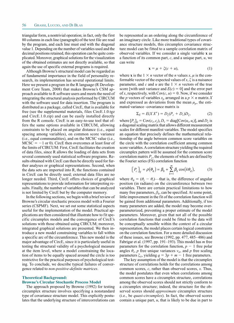
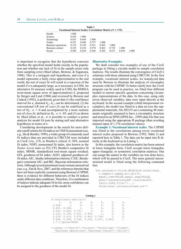
Example 1: Vocational interest scales. The CSPMF was fitted to the correlations among seven vocational interest scales proposed in Browne (1992, Table 2) and reported here in Table 1. The data can be input into R di-rectly at the keyboard as in Listing 1.
In this example, the correlation matrix has been entered in lower triangular form. CircE accepts lower triangular, upper triangular, or symmetric correlation matrices. One can assign the names to the variables (as was done here), which will be passed to CircE. The more general uncon-strained model is fitted using the following command line:
Voc.unconstr<-CircE.BFGS(R=R.vocational, v.names=v.names,m=1,N=175,equal.com=FALSE,equal.ang=FALSE,mcsc="unconstrained",iterlim=250,factr=1e06,file="/.../Vocational.unconstrained.txt")
is important to recognize that the hypothesis concerns whether the specified model holds exactly in the popula-tion and whether any lack of fit in the sample arises only from sampling error (MacCallum, Browne, & Sugawara, 1996). This is a stringent null hypothesis, and even if a model represents a fairly close approximation to the real world, the test of exact fit will result in a rejection of the model if n is adequately large, as is necessary in CSM. An alternative fit measure widely used in CSM, the RMSEA (root-mean square error of approximation) , proposed by Steiger and Lind (1980) and reviewed by Browne and Cudeck (1992), is preferred, given that (1) the confidence interval for , denoted L; U, can be determined; (2) the conventional LR test of exact fit can be redefined as a test of H0 : 0 and accompanied by a more realistic test of close fit, defined as H0 : .05; and (3) as shown by MacCallum et al., it is possible to conduct a power analysis for model fit tests by stating null and alternative hypotheses in terms of .
Considering developments in the search for more defi-nite cutoff criteria for fit indices in CSM fit assessment (see, e.g., Hu & Bentler, 1999), a wider group of commonly used fit indices than are provided in CIRCUM were included in CircE (viz., CN, or Hoelter’s critical N; NFI, normed fit index; NNFI, nonnormed fit index, also known as the Tucker–Lewis index or TLI; CFI, Bentler’s comparative fit index; SRMR, standardized root-mean square residual; GFI, goodness-of-fit index; AGFI, adjusted goodness-of-fit index; AIC, Akaike information criterion; CAIC, Bozdo-gan’s consistent AIC; and BIC, Bayesian information crite-rion). Although several prominent issues remain unresolved (see, e.g., Fan & Sivo, 2007, and the references therein) that have not been explicitly examined using Browne’s CSPMF, there is evidence for different behaviors of the fit indices under different data conditions. Therefore, if a combination of indices indicate adequate fit levels, more confidence can be assigned to the goodness of the model fit.
Table 1 Vocational Interest Scales: Correlation Matrix (N 175)
Health 1.000Science 0.654 1.000Technology 0.453 0.644 1.000Trades 0.251 0.440 0.757 1.000Business operations 0.122 0.158 0.551 0.493 1.000Business contact 0.218 0.210 0.570 0.463 0.754 1.000Social 0.496 0.264 0.366 0.202 0.471 0.650 1.000
Listing 1
R.vocational<-matrix(c( 1, 0, 0, 0, 0, 0, 0, 0.654, 1, 0, 0, 0, 0, 0, 0.453, 0.644, 1, 0, 0, 0, 0, 0.251, 0.440, 0.757, 1, 0, 0, 0, 0.122, 0.158, 0.551, 0.493, 1, 0, 0, 0.218, 0.210, 0.570, 0.463, 0.754, 1, 0, 0.496, 0.264, 0.366, 0.202, 0.471, 0.650, 1 ),7,7,byrow=TRUE)
v.names<-c("Health","Science","Technology","Trades", "Business Operations","Business Contact","Social”)
CIRCUMPLEX MODELS 59
Voc.eqspace<-CircE.BFGS(R=R.vocational,v.names=v.names,m=1,N=175,equal.com=FALSE,equal.ang=TRUE, mcsc="unconstrained",iterlim=250,factr=1e06,file="/.../Vocational.equal.space.txt")
The matrix depicted in Table 1 has nonnegative ele-ments. Clearly, there is a circular ordering of interest scales such that adjacent scales have high correlations. The correlations tend to decrease as the separation be-tween tests increases, but then they increase after an ideal distance of 180º of separation has been reached. Since the coefficients are positive, the value of 180º could be set to 0, imposing mcsc “0” (another possible option is
180º 1 for negative correlation coefficients). For the four fitted models, maximum likelihood estimates of polar angles and communality indices, estimated Fourier series weights, and fit measures (sample discrepancy function value F , population discrepancy function value F0, and RMSEA index ) are reported in Tables 2 and 3.
The results for m 1, m 2, and m 3 in Equation 3 coincide precisely with the ones obtained by CIRCUM. Particularly, as Browne (1992, p. 494) also reported, the FS correlation function with m 2 gave two Heywood cases, (xi,ci)
1, in the unconstrained model, and FS with m 3 resulted in a correlation function weight estimate,
3, attaining the lower bound of zero.Example 2: Child interpersonal circumplex. To
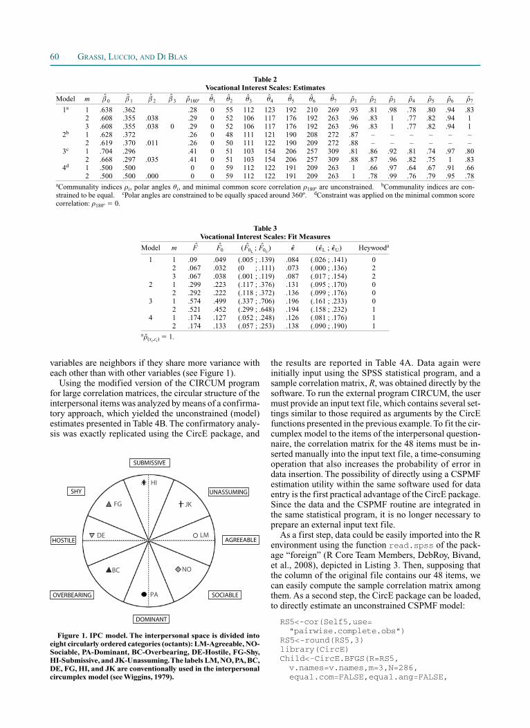
illustrate how CircE can be used to test the circumplex structure of dozens of variables (e.g., personality ques-tionnaire items), we applied CSPMF estimation to a re-cently collected data set to examine the structural conti-nuity of the interpersonal circumplex model in childhood (Di Blas, Grassi, Luccio, & Momentè, 2008). Specifically, we analyzed 286 self-reports provided by 5th-grade chil-dren who rated their interpersonal behavior on 48 items (i.e., six items for each of eight scale octants) conceptually organized around the dominance (DOM) and love (LOV) domains according to Wiggins’s interpersonal circumplex (IPC) model (Wiggins, 1979; Wiggins & Trapnell, 1996). Briefly, Wiggins’s model is based on the idea that people who interact attempt to negotiate relations of hierarchy and cooperation by granting or denying the resources of power (dominance) and warmth (love). Accordingly, the IPC model differently combines elements of the reference axes (DOM and LOV) and defines eight possible interper-sonal styles circularly ordered in terms of DOM and LOV, in compliance with a law of neighboring, positing that two
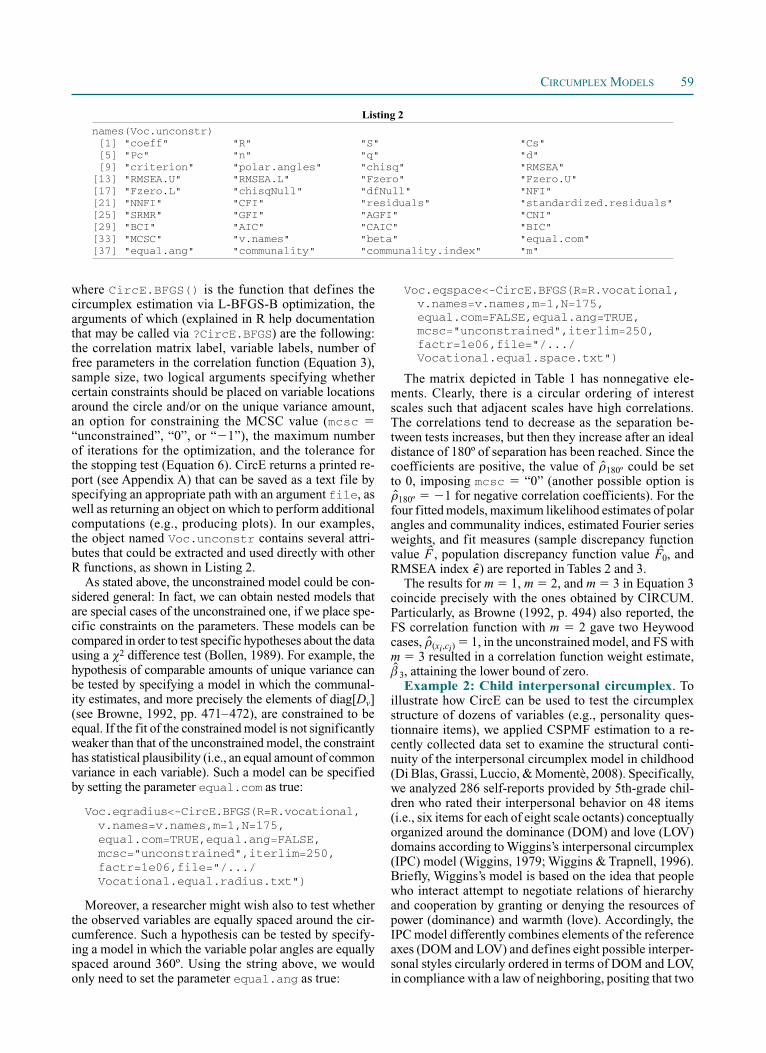
where CircE.BFGS() is the function that defines the circumplex estimation via L-BFGS-B optimization, the arguments of which (explained in R help documentation that may be called via ?CircE.BFGS) are the following: the correlation matrix label, variable labels, number of free parameters in the correlation function (Equation 3), sample size, two logical arguments specifying whether certain constraints should be placed on variable locations around the circle and/or on the unique variance amount, an option for constraining the MCSC value (mcsc “unconstrained”, “0”, or “ 1”), the maximum number of iterations for the optimization, and the tolerance for the stopping test (Equation 6). CircE returns a printed re-port (see Appendix A) that can be saved as a text file by specifying an appropriate path with an argument file, as well as returning an object on which to perform additional computations (e.g., producing plots). In our examples, the object named Voc.unconstr contains several attri-butes that could be extracted and used directly with other R functions, as shown in Listing 2.
As stated above, the unconstrained model could be con-sidered general: In fact, we can obtain nested models that are special cases of the unconstrained one, if we place spe-cific constraints on the parameters. These models can be compared in order to test specific hypotheses about the data using a 2 difference test (Bollen, 1989). For example, the hypothesis of comparable amounts of unique variance can be tested by specifying a model in which the communal-ity estimates, and more precisely the elements of diag[Dv] (see Browne, 1992, pp. 471–472), are constrained to be equal. If the fit of the constrained model is not significantly weaker than that of the unconstrained model, the constraint has statistical plausibility (i.e., an equal amount of common variance in each variable). Such a model can be specified by setting the parameter equal.com as true:
Voc.eqradius<-CircE.BFGS(R=R.vocational,v.names=v.names,m=1,N=175,equal.com=TRUE,equal.ang=FALSE, mcsc="unconstrained",iterlim=250,factr=1e06,file="/.../Vocational.equal.radius.txt")
Moreover, a researcher might wish also to test whether the observed variables are equally spaced around the cir-cumference. Such a hypothesis can be tested by specify-ing a model in which the variable polar angles are equally spaced around 360º. Using the string above, we would only need to set the parameter equal.ang as true:
Listing 2
names(Voc.unconstr) [1] "coeff" "R" "S" "Cs" [5] "Pc" "n" "q" "d" [9] "criterion" "polar.angles" "chisq" "RMSEA"[13] "RMSEA.U" "RMSEA.L" "Fzero" "Fzero.U"[17] "Fzero.L" "chisqNull" "dfNull" "NFI"[21] "NNFI" "CFI" "residuals" "standardized.residuals"[25] "SRMR" "GFI" "AGFI" "CNI"[29] "BCI" "AIC" "CAIC" "BIC"[33] "MCSC" "v.names" "beta" "equal.com"[37] "equal.ang" "communality" "communality.index" "m"
60 GRASSI, LUCCIO, AND DI BLAS
the results are reported in Table 4A. Data again were initially input using the SPSS statistical program, and a sample correlation matrix, R, was obtained directly by the software. To run the external program CIRCUM, the user must provide an input text file, which contains several set-tings similar to those required as arguments by the CircE functions presented in the previous example. To fit the cir-cumplex model to the items of the interpersonal question-naire, the correlation matrix for the 48 items must be in-serted manually into the input text file, a time- consuming operation that also increases the probability of error in data insertion. The possibility of directly using a CSPMF estimation utility within the same software used for data entry is the first practical advantage of the CircE package. Since the data and the CSPMF routine are integrated in the same statistical program, it is no longer necessary to prepare an external input text file.
As a first step, data could be easily imported into the R environment using the function read.spss of the pack-age “foreign” (R Core Team Members, DebRoy, Bivand, et al., 2008), depicted in Listing 3. Then, supposing that the column of the original file contains our 48 items, we can easily compute the sample correlation matrix among them. As a second step, the CircE package can be loaded, to directly estimate an unconstrained CSPMF model:
RS5<-cor(Self5,use="pairwise.complete.obs")
RS5<-round(RS5,3)library(CircE)Child<-CircE.BFGS(R=RS5,v.names=v.names,m=3,N=286,equal.com=FALSE,equal.ang=FALSE,
variables are neighbors if they share more variance with each other than with other variables (see Figure 1).
Using the modified version of the CIRCUM program for large correlation matrices, the circular structure of the interpersonal items was analyzed by means of a confirma-tory approach, which yielded the unconstrained (model) estimates presented in Table 4B. The confirmatory analy-sis was exactly replicated using the CircE package, and
Table 2 Vocational Interest Scales: Estimates
Model m 0 1 2 3 180º
1 2 3 4 5 6 7 1 2 3 4 5 6 7
1a 1 .638 .362 .28 0 55 112 123 192 210 269 .93 .81 .98 .78 .80 .94 .832 .608 .355 .038 .29 0 52 106 117 176 192 263 .96 .83 1 .77 .82 .94 13 .608 .355 .038 0 .29 0 52 106 117 176 192 263 .96 .83 1 .77 .82 .94 1
2b 1 .628 .372 .26 0 48 111 121 190 208 272 .87 – – – – – –2 .619 .370 .011 .26 0 50 111 122 190 209 272 .88 – – – – – –
3c 1 .704 .296 .41 0 51 103 154 206 257 309 .81 .86 .92 .81 .74 .97 .802 .668 .297 .035 .41 0 51 103 154 206 257 309 .88 .87 .96 .82 .75 1 .83
4d 1 .500 .500 0 0 59 112 122 191 209 263 1 .66 .97 .64 .67 .91 .662 .500 .500 .000 0 0 59 112 122 191 209 263 1 .78 .99 .76 .79 .95 .78
aCommunality indices i, polar angles i, and minimal common score correlation 180º are unconstrained. bCommunality indices are con-strained to be equal. cPolar angles are constrained to be equally spaced around 360º. dConstraint was applied on the minimal common score correlation: 180º 0.
Table 3 Vocational Interest Scales: Fit Measures
Model m F F0 (F0L ; F0U
) ( L ; U) Heywooda
1 1 .09 .049 (.005 ; .139) .084 (.026 ; .141) 02 .067 .032 (0 ; .111) .073 (.000 ; .136) 23 .067 .038 (.001 ; .119) .087 (.017 ; .154) 2
2 1 .299 .223 (.117 ; .376) .131 (.095 ; .170) 02 .292 .222 (.118 ; .372) .136 (.099 ; .176) 0
3 1 .574 .499 (.337 ; .706) .196 (.161 ; .233) 02 .521 .452 (.299 ; .648) .194 (.158 ; .232) 1
4 1 .174 .127 (.052 ; .248) .126 (.081 ; .176) 12 .174 .133 (.057 ; .253) .138 (.090 ; .190) 1
a(xi,ci)
1.
LM
JK
HI
FG
DE
BC
PA
NO
DOMINANT
AGREEABLE
SUBMISSIVE
HOSTILE
OVERBEARING SOCIABLE
UNASSUMINGSHY
Figure 1. IPC model. The interpersonal space is divided into eight circularly ordered categories (octants): LM-Agreeable, NO-Sociable, PA-Dominant, BC-Overbearing, DE-Hostile, FG-Shy, HI-Submissive, and JK-Unassuming. The labels LM, NO, PA, BC, DE, FG, HI, and JK are conventionally used in the interpersonal circumplex model (see Wiggins, 1979).

CIRCUMPLEX MODELS 61
a vector of the same length containing the point char-acters (point.char),
point.char=c(21,23,16,17,25,24,8,3)
and a vector of color names for filling in the points (bg.point).
bg.point=c("white","gray40","black","black","gray80","gray60","black","black")
The char.assign() function matches scale names with the item names (the vector v.names) and assigns appro-priate characters and colors automatically. The result is an R object (A) that contains two vectors of the same length, shown in Listing 4, of variable names that will be passed to CircE.Plot().
Octant-bounded estimation. For the previous exam-ple, child interpersonal circumplex, quantitative model-fitting indices (Table 4A, first row) showed that the 5th
mcsc="unconstrained",iterlim=250,factr=1e10)
As anticipated, another notable practical advantage is the possibility to produce a graphical representation of the es-timated circular order using the function CircE.Plot() (see Figure 2).
To simplify the assignment of a color and character type to each point on the graph—both of which are required as arguments by the function CircE.Plot()—in the case of a large number of items, the function char.assign() can be used as follows:
Supposing that the items are tagged with reference to the relative scale (e.g., Table 4A, first column), it is sufficient to create a string with scale names (sc.names),
sc.names=c("LM","NO","PA","BC","DE","FG","HI","JK")
Listing 3
library(foreign)Self5<-read.spss("SELF5.sav",to.data.frame=TRUE,use.value.label=FALSE)v.names<-names(Self5)v.names [1] "1LM" "43JK" "5FG" "9LM" "8DE" "4PA" "14BC" "2NO" "17LM" "25LM" [11] "21FG" "6BC" "18NO" "16DE" "42NO" "3JK" "23HI" "41LM" "28PA" "38BC" [21] "20PA" "24DE" "26NO" "27JK" "29FG" "40DE" "12PA" "22BC" "11JK" "7HI" [31] "33LM" "31HI" "19JK" "48DE" "13FG" "35JK" "30BC" "44PA" "39HI" "32DE" [41] "47HI" "45FG" "46BC" "34NO" "37FG" "15HI" "36PA" "10NO"
Attended Circular Order
LM NO PA BC DE FG HI JK
180º 0.63max h 0.71max h2 0.5
d
0 45 90 135 180 225 270 315 360
1.0
0.5
0.0
0.5
1.0
( d) 0 mk 1 kcos (k d)
180º 0.63
3 0.1161
2 0.0765
1 0.699
0 0.1084
Figure 2. Child interpersonal circumplex: Unconstrained circular ordering of the 48 items, obtained using the CircE.Plot function.

62 GRASSI, LUCCIO, AND DI BLAS
interpersonal variables overlap (e.g., JK and HI sentences) and that items representing the same interpersonal variable are not regularly distributed within 45º arcs, as the ICM posits (e.g., FG items are spread through the upper left quadrant, but DE, BC, and PA sentences are all arranged within the lower left quadrant). Therefore, whatever deci-sion we make about the structural validity of our 48-item measure, such a decision would be based on personal judg-ments. Conversely, we primarily need to test whether each item represents what it is intended to represent, and thereby whether it falls within an expected (45º) arc.
graders’ ratings conformed to a circumplex structure; that is, the 48 sentences could be represented in a circular array. Nevertheless, to develop a psychological measure, we need to demonstrate that each item represents the intended vari-able, in agreement with the psychological model, in order to provide evidence of the measure’s structural validity. To help with this aim, we may inspect the item continuum il-lustrated in Figure 2. Overall, the observed sentence array seems to reproduce fairly well the hypothesized circular array shown in Figure 1. A closer inspection, however, re-veals that some sentences intended to represent different
Table 4 Estimates of Unknown Parameters: Comparison Between the Two Programs
(A) CircE (B) CIRCUM
F F0 (F0L ; F0U
) ( L ; U) F F0 (F0L ; F0U
) ( L ; U)
5.86 2.27 (1.90 ; 2.68) .047 (.043 ; .051) 5.86 2.25 (1.87 ; 2.65) .047 (.043 ; .051)
i ( iL ; iU
) (x,c) ( L ; U) i ( iL ; iU
) (x,c) ( L ; U)
1LM 0 (0 ; 0) .44 (.34 ; .56) 1LM 0 (0 ; 0) .45 (.34 ; .56)27JK 23 (5 ; 41) .43 (.32 ; .55) 27JK 23 (5 ; 41) .43 (.33 ; .55)3JK 33 (15 ; 51) .45 (.34 ; .56) 3JK 33 (15 ; 50) .45 (.35 ; .57)31HI 37 (16 ; 59) .33 (.23 ; .47) 31HI 37 (16 ; 58) .34 (.24 ; .48)43JK 38 (18 ; 58) .37 (.26 ; .50) 43JK 38 (18 ; 57) .38 (.27 ; .51)35JK 39 (21 ; 56) .49 (.39 ; .60) 35JK 38 (21 ; 55) .48 (.38 ; .60)11JK 44 (26 ; 61) .48 (.38 ; .60) 11JK 44 (26 ; 61) .48 (.38 ; .60)15HI 46 (27 ; 66) .40 (.30 ; .53) 15HI 46 (27 ; 65) .42 (.31 ; .54)39HI 49 (31 ; 66) .47 (.37 ; .59) 39HI 48 (30 ; 65) .48 (.37 ; .59)19JK 58 (35 ; 82) .31 (.20 ; .45) 19JK 57 (33 ; 82) .29 (.18 ; .44)47HI 83 (62 ; 103) .37 (.27 ; .51) 47HI 83 (62 ; 103) .38 (.27 ; .51)23HI 83 (67 ; 100) .55 (.45 ; .66) 23HI 83 (67 ; 100) .56 (.46 ; .67)7HI 84 (66 ; 101) .51 (.40 ; .62) 7HI 83 (66 ; 101) .51 (.41 ; .63)29FG 87 (63 ; 111) .29 (.19 ; .44) 29FG 87 (61 ; 112) .26 (.16 ; .42)21FG 95 (79 ; 112) .56 (.46 ; .67) 21FG 95 (78 ; 112) .56 (.46 ; .66)24DE 103 (80 ; 126) .32 (.21 ; .46) 24DE 103 (80 ; 125) .32 (.21 ; .46)13FG 128 (112 ; 144) .71 (.62 ; .79) 13FG 128 (112 ; 144) .71 (.62 ; .79)5FG 131 (115 ; 148) .63 (.54 ; .72) 5FG 131 (115 ; 148) .63 (.54 ; .72)37FG 136 (120 ; 152) .67 (.58 ; .75) 37FG 136 (120 ; 152) .67 (.58 ; .75)45FG 156 (139 ; 173) .50 (.40 ; .61) 45FG 155 (138 ; 172) .50 (.39 ; .61)48DE 183 (167 ; 199) .56 (.47 ; .66) 48DE 183 (167 ; 200) .56 (.47 ; .66)16DE 184 (166 ; 201) .47 (.37 ; .58) 16DE 184 (166 ; 201) .47 (.37 ; .58)8DE 190 (174 ; 207) .55 (.45 ; .64) 8DE 190 (173 ; 206) .55 (.46 ; .65)38BC 195 (179 ; 211) .59 (.50 ; .68) 38BC 195 (179 ; 211) .59 (.50 ; .68)40DE 195 (175 ; 216) .37 (.27 ; .50) 40DE 195 (175 ; 216) .38 (.28 ; .50)32DE 197 (181 ; 213) .61 (.53 ; .70) 32DE 197 (181 ; 213) .61 (.53 ; .70)14BC 208 (190 ; 225) .51 (.41 ; .61) 14BC 207 (190 ; 224) .51 (.41 ; .61)22BC 213 (194 ; 232) .44 (.34 ; .55) 22BC 213 (194 ; 232) .43 (.33 ; .54)46BC 218 (203 ; 234) .70 (.62 ; .77) 46BC 218 (203 ; 233) .70 (.62 ; .77)6BC 221 (205 ; 237) .62 (.53 ; .71) 6BC 221 (205 ; 236) .62 (.54 ; .71)30BC 229 (207 ; 250) .34 (.24 ; .47) 30BC 229 (207 ; 250) .35 (.25 ; .48)20PA 246 (224 ; 267) .34 (.23 ; .48) 20PA 246 (225 ; 267) .35 (.24 ; .48)4PA 248 (226 ; 270) .33 (.22 ; .47) 4PA 249 (227 ; 270) .33 (.22 ; .47)36PA 251 (235 ; 267) .64 (.54 ; .73) 36PA 251 (235 ; 266) .64 (.54 ; .73)44PA 252 (235 ; 269) .53 (.43 ; .64) 44PA 252 (235 ; 269) .53 (.42 ; .63)12PA 268 (249 ; 287) .43 (.32 ; .55) 12PA 268 (249 ; 287) .42 (.31 ; .54)18NO 286 (268 ; 304) .49 (.39 ; .61) 18NO 286 (268 ; 304) .49 (.39 ; .60)28PA 293 (275 ; 311) .47 (.37 ; .59) 28PA 292 (274 ; 311) .47 (.36 ; .58)42NO 294 (274 ; 314) .41 (.31 ; .54) 42NO 293 (274 ; 313) .42 (.31 ; .54)34NO 295 (279 ; 312) .59 (.49 ; .69) 34NO 295 (278 ; 311) .59 (.49 ; .69)26NO 303 (284 ; 321) .46 (.36 ; .58) 26NO 302 (283 ; 320) .46 (.36 ; .58)2NO 305 (288 ; 323) .50 (.39 ; .61) 2NO 304 (287 ; 322) .50 (.40 ; .61)10NO 326 (308 ; 344) .44 (.33 ; .56) 10NO 325 (307 ; 343) .43 (.33 ; .56)33LM 347 (328 ; 6) .39 (.29 ; .52) 33LM 346 (328 ; 5) .41 (.31 ; .53)41LM 349 (334 ; 5) .58 (.48 ; .67) 41LM 349 (334 ; 4) .58 (.48 ; .67)17LM 354 (339 ; 9) .57 (.48 ; .67) 17LM 354 (338 ; 9) .57 (.48 ; .67)9LM 357 (342 ; 12) .60 (.51 ; .69) 9LM 356 (341 ; 11) .60 (.51 ; .69)25LM 357 (342 ; 11) .66 (.58 ; .74) 25LM 356 (342 ; 11) .67 (.58 ; .75)
CPU time 36 min CPU time 27 min

CIRCUMPLEX MODELS 63
lower<-c(-22.5,292.5,247.5,202.5,157.5, 112.5,67.5,22.5)upper<-c(22.5,337.5,292.5,247.5,202.5, 157.5,112.5,67.5)B<-bound.assign(sc.names,v.names, lower,upper)Child.obm<-CircE.BFGS(R=RS5, v.names=v.names,m=3,N=286, equal.com=FALSE,equal.ang=FALSE, mcsc="unconstrained",iterlim=250, factr=1e10,upper=B$upper,lower=B$lower)
The estimated octant-bounded angular position can be graphically represented (see Figure 3) using the function CircE.Plot(), as in the previous example.
The models that can be tested with CIRCUM do not serve this purpose. Thus, we developed a function aimed at testing a model in which items are constrained to fall within a given arc, but within that arc, each item’s angular position and radius are unconstrained. The function CircE.BFGS has two arguments, upper and lower, which specify, respectively, the upper and lower bounds for each item, or variable, used for a bounded optimization; a bound as-signment functionality, bound.assign(), helps provide each of the 48 items with an upper and lower bound, as seen previously for char.assign(). The code in R for fitting the octant-bounded model is:
sc.names=c("LM","NO","PA","BC","DE", "FG","HI","JK")
Listing 4
A<-char.assign(sc.names, v.names, point.char, bg.point) A $pchar [1] 21 3 24 21 25 16 17 23 21 21 24 17 23 25 23 3 8 21 16 17 16 25 23 3 [25] 24 25 16 17 3 8 21 8 3 25 24 3 17 16 8 25 8 24 17 23 24 8 16 23
$bg.points [1] "white" "black" "gray60" "white" "gray80" "black" "black" "gray40" [9] "white" "white" "gray60" "black" "gray40" "gray80" "gray40" "black" [17] "black" "white" "black" "black" "black" "gray80" "gray40" "black" [25] "gray60" "gray80" "black" "black" "black" "black" "white" "black" [33] "black" "gray80" "gray60" "black" "black" "black" "black" "gray80" [41] "black" "gray60" "black" "gray40" "gray60" "black" "black" "gray40"CircE.Plot(Child,pchar=A$pchar,bg.points=A$bg.points,big.points=60, big.labels=40,bg.plot="white",col.text="black",twodim=FALSE, labels=FALSE)
Attended Circular Order
LM NO PA BC DE FG HI JK
180º 0.649max h 0.71max h2 0.50
d
0 45 90 135 180 225 270 315 360
1.0
0.5
0.0
0.5
1.0
3 0.0865
2 0.065
1 0.7378
0 0.1107
( d) 0 mk 1 kcos (k d)
180º 0.649
Figure 3. Child interpersonal circumplex: Octant-bounded circular ordering of the 48 items.
64 GRASSI, LUCCIO, AND DI BLAS
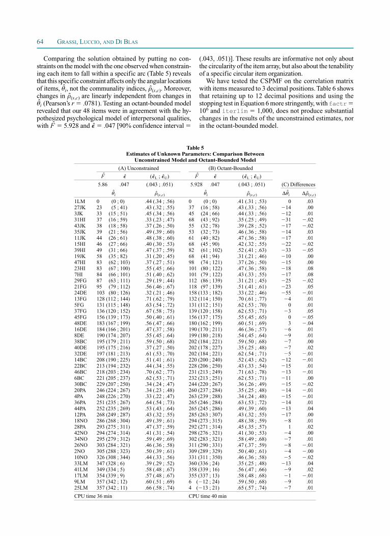
(.043, .051)]. These results are informative not only about the circularity of the item array, but also about the tenability of a specific circular item organization.
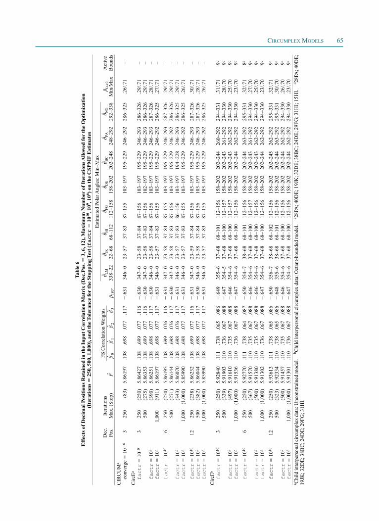
We have tested the CSPMF on the correlation matrix with items measured to 3 decimal positions. Table 6 shows that retaining up to 12 decimal positions and using the stopping test in Equation 6 more stringently, with factr 106 and iterlim 1,000, does not produce substantial changes in the results of the unconstrained estimates, nor in the octant-bounded model.
Comparing the solution obtained by putting no con-straints on the model with the one observed when constrain-ing each item to fall within a specific arc (Table 5) reveals that this specific constraint affects only the angular locations of items, i, not the communality indices, (x,c). Moreover, changes in (x,c) are linearly independent from changes in
i (Pearson’s r .0781). Testing an octant-bounded model revealed that our 48 items were in agreement with the hy-pothesized psychological model of interpersonal qualities, with F 5.928 and .047 [90% confidence interval
Table 5 Estimates of Unknown Parameters: Comparison Between
Unconstrained Model and Octant-Bounded Model
(A) Unconstrained (B) Octant-Bounded
F ( L ; U) F ( L ; U)
5.86 .047 (.043 ; .051) 5.928 .047 (.043 ; .051) (C) Differences
i (x,c) i (x,c) i (x,c)
1LM 0 (0 ; 0) .44 (.34 ; .56) 0 (0 ; 0) .41 (.31 ; .53) 0 .0327JK 23 (5 ; 41) .43 (.32 ; .55) 37 (16 ; 58) .43 (.33 ; .56) 14 .003JK 33 (15 ; 51) .45 (.34 ; .56) 45 (24 ; 66) .44 (.33 ; .56) 12 .0131HI 37 (16 ; 59) .33 (.23 ; .47) 68 (43 ; 92) .35 (.25 ; .49) 31 .0243JK 38 (18 ; 58) .37 (.26 ; .50) 55 (32 ; 78) .39 (.28 ; .52) 17 .0235JK 39 (21 ; 56) .49 (.39 ; .60) 53 (32 ; 73) .46 (.36 ; .58) 14 .0311JK 44 (26 ; 61) .48 (.38 ; .60) 61 (40 ; 82) .47 (.36 ; .58) 17 .0115HI 46 (27 ; 66) .40 (.30 ; .53) 68 (45 ; 90) .42 (.32 ; .55) 22 .0239HI 49 (31 ; 66) .47 (.37 ; .59) 82 (61 ; 102) .52 (.41 ; .63) 33 .0519JK 58 (35 ; 82) .31 (.20 ; .45) 68 (41 ; 94) .31 (.21 ; .46) 10 .0047HI 83 (62 ; 103) .37 (.27 ; .51) 98 (74 ; 121) .37 (.26 ; .50) 15 .0023HI 83 (67 ; 100) .55 (.45 ; .66) 101 (80 ; 122) .47 (.36 ; .58) 18 .087HI 84 (66 ; 101) .51 (.40 ; .62) 101 (79 ; 122) .43 (.33 ; .55) 17 .0829FG 87 (63 ; 111) .29 (.19 ; .44) 112 (86 ; 139) .31 (.21 ; .45) 25 .0221FG 95 (79 ; 112) .56 (.46 ; .67) 118 (97 ; 139) .51 (.41 ; .61) 23 .0524DE 103 (80 ; 126) .32 (.21 ; .46) 158 (133 ; 182) .33 (.22 ; .46) 55 .0113FG 128 (112 ; 144) .71 (.62 ; .79) 132 (114 ; 150) .70 (.61 ; .77) 4 .015FG 131 (115 ; 148) .63 (.54 ; .72) 131 (112 ; 151) .62 (.53 ; .70) 0 .0137FG 136 (120 ; 152) .67 (.58 ; .75) 139 (120 ; 158) .62 (.53 ; .71) 3 .0545FG 156 (139 ; 173) .50 (.40 ; .61) 156 (137 ; 175) .55 (.45 ; .65) 0 .0548DE 183 (167 ; 199) .56 (.47 ; .66) 180 (162 ; 199) .60 (.51 ; .69) 3 .0416DE 184 (166 ; 201) .47 (.37 ; .58) 190 (170 ; 211) .46 (.36 ; .57) 6 .018DE 190 (174 ; 207) .55 (.45 ; .64) 199 (180 ; 218) .54 (.45 ; .64) 9 .0138BC 195 (179 ; 211) .59 (.50 ; .68) 202 (184 ; 221) .59 (.50 ; .68) 7 .0040DE 195 (175 ; 216) .37 (.27 ; .50) 202 (178 ; 227) .35 (.25 ; .48) 7 .0232DE 197 (181 ; 213) .61 (.53 ; .70) 202 (184 ; 221) .62 (.54 ; .71) 5 .0114BC 208 (190 ; 225) .51 (.41 ; .61) 220 (200 ; 240) .52 (.43 ; .62) 12 .0122BC 213 (194 ; 232) .44 (.34 ; .55) 228 (206 ; 250) .43 (.33 ; .54) 15 .0146BC 218 (203 ; 234) .70 (.62 ; .77) 231 (213 ; 249) .71 (.63 ; .78) 13 .016BC 221 (205 ; 237) .62 (.53 ; .71) 232 (213 ; 251) .62 (.53 ; .71) 11 .0030BC 229 (207 ; 250) .34 (.24 ; .47) 244 (220 ; 267) .36 (.26 ; .49) 15 .0220PA 246 (224 ; 267) .34 (.23 ; .48) 260 (237 ; 284) .35 (.25 ; .48) 14 .014PA 248 (226 ; 270) .33 (.22 ; .47) 263 (239 ; 288) .34 (.24 ; .48) 15 .0136PA 251 (235 ; 267) .64 (.54 ; .73) 265 (246 ; 284) .63 (.53 ; .72) 14 .0144PA 252 (235 ; 269) .53 (.43 ; .64) 265 (245 ; 286) .49 (.39 ; .60) 13 .0412PA 268 (249 ; 287) .43 (.32 ; .55) 285 (263 ; 307) .43 (.32 ; .55) 17 .0018NO 286 (268 ; 304) .49 (.39 ; .61) 294 (273 ; 315) .48 (.38 ; .59) 8 .0128PA 293 (275 ; 311) .47 (.37 ; .59) 292 (271 ; 314) .45 (.35 ; .57) 1 .0242NO 294 (274 ; 314) .41 (.31 ; .54) 298 (276 ; 321) .41 (.30 ; .53) 4 .0034NO 295 (279 ; 312) .59 (.49 ; .69) 302 (283 ; 321) .58 (.49 ; .68) 7 .0126NO 303 (284 ; 321) .46 (.36 ; .58) 311 (290 ; 331) .47 (.37 ; .59) 8 .012NO 305 (288 ; 323) .50 (.39 ; .61) 309 (289 ; 329) .50 (.40 ; .61) 4 .0010NO 326 (308 ; 344) .44 (.33 ; .56) 331 (311 ; 350) .46 (.36 ; .58) 5 .0233LM 347 (328 ; 6) .39 (.29 ; .52) 360 (336 ; 24) .35 (.25 ; .48) 13 .0441LM 349 (334 ; 5) .58 (.48 ; .67) 358 (339 ; 16) .56 (.47 ; .66) 9 .0217LM 354 (339 ; 9) .57 (.48 ; .67) 355 (337 ; 13) .58 (.48 ; .68) 1 .019LM 357 (342 ; 12) .60 (.51 ; .69) 6 ( 12 ; 24) .59 (.50 ; .68) 9 .0125LM 357 (342 ; 11) .66 (.58 ; .74) 4 ( 13 ; 21) .65 (.57 ; .74) 7 .01
CPU time 36 min CPU time 40 min
CIRCUMPLEX MODELS 65
Tab
le 6
E
ffec
ts o
f D
ecim
al P
osit
ion
s R
etai
ned
in t
he
Inp
ut
Cor
rela
tion
Mat
rix
(Dec
.Pos
. 3
, 6, 1
2), M
axim
um
Nu
mb
er o
f It
erat
ion
s All
owed
for
the
Op
tim
izat
ion
(I
tera
tion
s 2
50, 5
00, 1
,000
), a
nd
th
e T
oler
ance
for
the
Sto
pp
ing
Tes
t (factr
1
010, 1
09 , 1
06 ) o
n t
he
CS
PM
F E
stim
ates
Est
imat
ed P
olar
Ang
les:
Min
–Max
Dec
.It
erat
ions
FS
Cor
rela
tion
Wei
ghts
LM
JKH
IF
GD
EB
C
PA
NO
(x
,c)
Act
ive
Pos.
M
ax. (
Sto
p)
F
0
1
2
3
180º
33
8–22
22
–68
68
–112
11
2–15
8
158–
202
20
2–24
8
248–
292
29
2–33
8
Min
/Max
B
ound
s
CIR
CU
Ma
co
nver
ge
10
6 3
250
(83)
5.86
197
.108
.698
.077
.117
.631
346
–0
23–5
737
–83
87–1
5510
3–19
719
5–22
924
6–2
9228
6–3
25.2
6/.7
1–
Cir
cEa
factr
1
010
325
0(2
50)
5.86
427
.108
.699
.077
.116
.630
347–
023
–58
37–8
487
–156
103–
197
195–
229
246
–293
286
–326
.29/
.71
–50
0(2
75)
5.86
353
.108
.699
.077
.116
.630
347–
023
–58
37–8
387
–156
102–
197
195–
229
246
–293
286
–326
.29/
.71
– factr
1
09(3
90)
5.86
251
.108
.698
.077
.117
.630
346
–0
23–5
837
–84
87–1
5610
3–19
719
5–22
924
6–2
9328
7–32
6.2
8/.7
1–
factr
1
061,
000
(911
)5.
8619
7.1
08.6
98.0
77.1
17.6
3134
6–
023
–57
37–8
387
–155
103–
197
195–
229
246
–292
286
–325
.27/
.71
–
factr
1
010
625
0(2
50)
5.86
195
.108
.699
.076
.116
.631
347–
023
–58
37–8
487
–155
103–
197
195–
229
246
–293
287–
326
.29/
.71
–50
0(2
71)
5.86
144
.108
.698
.076
.117
.630
347–
023
–58
37–8
387
–156
103–
197
195–
229
246
–292
286
–326
.29/
.71
– factr
1
09(3
43)
5.86
070
.108
.698
.076
.117
.631
346
–0
23–5
737
–83
86–1
5610
3–19
719
4–2
2824
6–2
9328
6–3
25.2
9/.7
1–
factr
1
061,
000
(1,0
00)
5.85
990
.108
.698
.077
.117
.631
346
–0
23–5
737
–83
87–1
5510
3–19
719
5–22
924
6–2
9228
6–3
25.2
6/.7
1–
factr
1
010
1225
0(2
38)
5.86
232
.108
.699
.077
.116
.631
347–
023
–59
37–8
487
–156
103–
197
195–
229
246
–293
287–
326
.30/
.71
– factr
1
0950
0(3
82)
5.86
044
.108
.698
.077
.117
.630
346
–0
23–5
837
–84
87–1
5610
3–19
719
5–22
924
6–2
9328
7–32
6.2
8/.7
1–
factr
1
061,
000
(1,0
00)
5.85
990
.108
.698
.077
.117
.631
346
–0
23–5
737
–83
87–1
5510
3–19
719
5–22
924
6–2
9228
6–3
25.2
6/.7
1–
Cir
cEb
factr
1
010
325
0(2
50)
5.92
840
.111
.738
.065
.086
.649
355–
637
–68
68–1
0111
2–15
615
8–20
220
2–24
426
0–2
9229
4–3
31.3
1/.7
19c
500
(339
)5.
9190
3.1
10.7
36.0
67.0
88.6
4735
4–5
37–
6868
–100
112–
157
158–
202
202–
243
261–
292
294
–330
.28/
.70
9c
factr
1
09(4
97)
5.91
610
.110
.735
.067
.088
.646
354
–6
37–
6868
–100
112–
157
158–
202
202–
243
262–
292
294
–330
.25/
.70
9c
factr
1
061,
000
(1,0
00)
5.91
536
.110
.736
.067
.088
.647
354
–6
37–
6868
–100
112–
156
158–
202
202–
244
262–
292
294
–330
.23/
.70
9c
factr
1
010
625
0(2
50)
5.92
770
.111
.738
.064
.087
.650
354
–738
–68
68–1
0111
2–15
615
8–20
220
2–24
426
3–29
229
5–33
1.3
2/.7
18d
500
(367
)5.
9157
0.1
10.7
35.0
67.0
88.6
4635
4–
637
–68
68–1
0011
2–15
715
8–20
220
2–24
326
1–29
229
4–3
30.2
7/.7
09c
factr
1
09(5
00)
5.91
380
.110
.735
.067
.088
.646
354
–6
37–
6868
–100
112–
156
158–
202
202–
243
262–
292
294
–330
.25/
.70
9c
factr
1
061,
000
(1,0
00)
5.91
302
.110
.736
.067
.088
.647
354
–6
37–
6868
–100
112–
156
158–
202
202–
244
262–
292
294
–330
.23/
.70
9c
factr
1
010
1225
0(2
50)
5.93
613
.111
.738
.065
.086
.650
356
–738
–68
68–1
0211
2–15
615
8–20
220
2–24
526
2–29
229
5–33
1.3
2/.7
19c
500
(323
)5.
9233
4.1
10.7
38.0
65.0
86.6
4835
5–6
38–
6868
–101
112–
156
158–
202
202–
244
263–
292
295–
331
.30/
.70
9c
factr
1
09(5
00)
5.91
457
.110
.735
.067
.088
.646
354
–6
37–
6868
–100
112–
156
158–
202
202–
244
262–
292
294
–330
.26/
.70
9c
factr
1
061,
000
(1,0
00)
5.91
301
.110
.736
.067
.088
.647
354
–6
37–
6868
–100
112–
156
158–
202
202–
244
262–
292
294
–330
.23/
.70
9ca C
hild
inte
rper
sona
l cir
cum
plex
dat
a: U
ncon
stra
ined
mod
el.
b Chi
ld in
terp
erso
nal c
ircu
mpl
ex d
ata:
Oct
ant-
boun
ded
mod
el.
c 28PA
; 40D
E; 1
9JK
; 32D
E; 3
8BC
; 24D
E; 2
9FG
; 31H
I; 1
5HI.
d 28
PA; 4
0DE
; 19
JK; 3
2DE
; 38B
C; 2
4DE
; 29F
G; 3
1HI.
66 GRASSI, LUCCIO, AND DI BLAS
of how to deal with matrices that are not positive definite is contained in the seminal work of Wothke (1993). What follows are ways to recover from such failures using the CircE program.
Sample covariance/correlation matrix is non- positive-definite. A non-positive-definite input matrix may signal a perfect linear dependency (collinearity) among the observed variables. Collinearity may be a result of one of the following factors: (1) a composite or total- score variable that is a sum of two or more component variables, all of which are included in the covariance ma-trix; (2) outliers or extreme observations; (3) a sample size that is smaller than the number of observed variables; or (4) error in transcribing a matrix. When the sample size is small, a sample covariance or correlation matrix may fail to be positive definite merely due to sampling fluctuation. Moreover, non-positive-definiteness of the input matrix typically occurs when the pairwise (rather than listwise) deletion method is used for handling missing data.
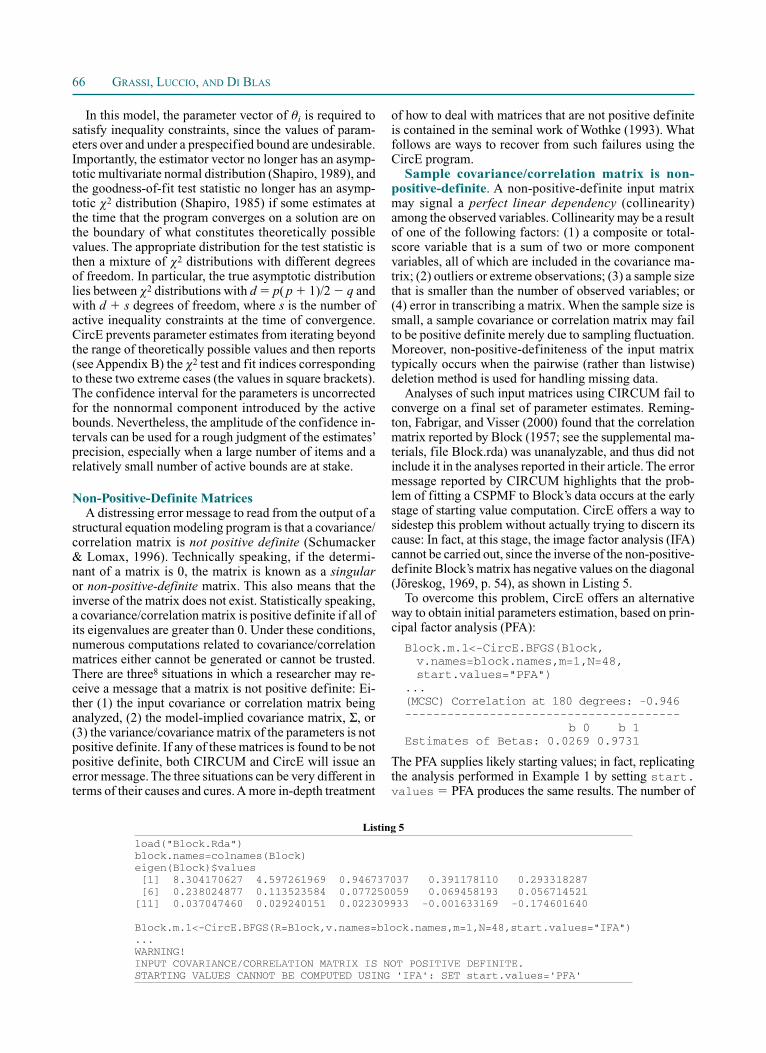
Analyses of such input matrices using CIRCUM fail to converge on a final set of parameter estimates. Reming-ton, Fabrigar, and Visser (2000) found that the correlation matrix reported by Block (1957; see the supplemental ma-terials, file Block.rda) was unanalyzable, and thus did not include it in the analyses reported in their article. The error message reported by CIRCUM highlights that the prob-lem of fitting a CSPMF to Block’s data occurs at the early stage of starting value computation. CircE offers a way to sidestep this problem without actually trying to discern its cause: In fact, at this stage, the image factor analysis (IFA) cannot be carried out, since the inverse of the non-positive-definite Block’s matrix has negative values on the diagonal (Jöreskog, 1969, p. 54), as shown in Listing 5.
To overcome this problem, CircE offers an alternative way to obtain initial parameters estimation, based on prin-cipal factor analysis (PFA):
Block.m.1<-CircE.BFGS(Block, v.names=block.names,m=1,N=48, start.values="PFA") ...(MCSC) Correlation at 180 degrees: -0.946--------------------------------------- b 0 b 1Estimates of Betas: 0.0269 0.9731
The PFA supplies likely starting values; in fact, replicating the analysis performed in Example 1 by setting start.values PFA produces the same results. The number of
In this model, the parameter vector of i is required to satisfy inequality constraints, since the values of param-eters over and under a prespecified bound are undesirable. Importantly, the estimator vector no longer has an asymp-totic multivariate normal distribution (Shapiro, 1989), and the goodness-of-fit test statistic no longer has an asymp-totic 2 distribution (Shapiro, 1985) if some estimates at the time that the program converges on a solution are on the boundary of what constitutes theoretically possible values. The appropriate distribution for the test statistic is then a mixture of 2 distributions with different degrees of freedom. In particular, the true asymptotic distribution lies between 2 distributions with d p( p 1)/2 q and with d s degrees of freedom, where s is the number of active inequality constraints at the time of convergence. CircE prevents parameter estimates from iterating beyond the range of theoretically possible values and then reports (see Appendix B) the 2 test and fit indices corresponding to these two extreme cases (the values in square brackets). The confidence interval for the parameters is uncorrected for the nonnormal component introduced by the active bounds. Nevertheless, the amplitude of the confidence in-tervals can be used for a rough judgment of the estimates’ precision, especially when a large number of items and a relatively small number of active bounds are at stake.
Non-Positive-Definite MatricesA distressing error message to read from the output of a
structural equation modeling program is that a covariance/correlation matrix is not positive definite (Schumacker & Lomax, 1996). Technically speaking, if the determi-nant of a matrix is 0, the matrix is known as a singular or non- positive-definite matrix. This also means that the inverse of the matrix does not exist. Statistically speaking, a covariance/ correlation matrix is positive definite if all of its eigenvalues are greater than 0. Under these conditions, numerous computations related to covariance/correlation matrices either cannot be generated or cannot be trusted. There are three8 situations in which a researcher may re-ceive a message that a matrix is not positive definite: Ei-ther (1) the input covariance or correlation matrix being analyzed, (2) the model-implied covariance matrix, , or (3) the variance/covariance matrix of the parameters is not positive definite. If any of these matrices is found to be not positive definite, both CIRCUM and CircE will issue an error message. The three situations can be very different in terms of their causes and cures. A more in-depth treatment
Listing 5
load("Block.Rda")block.names=colnames(Block)eigen(Block)$values [1] 8.304170627 4.597261969 0.946737037 0.391178110 0.293318287 [6] 0.238024877 0.113523584 0.077250059 0.069458193 0.056714521[11] 0.037047460 0.029240151 0.022309933 -0.001633169 -0.174601640
Block.m.1<-CircE.BFGS(R=Block,v.names=block.names,m=1,N=48,start.values="IFA")...WARNING!INPUT COVARIANCE/CORRELATION MATRIX IS NOT POSITIVE DEFINITE.STARTING VALUES CANNOT BE COMPUTED USING 'IFA': SET start.values='PFA'
CIRCUMPLEX MODELS 67
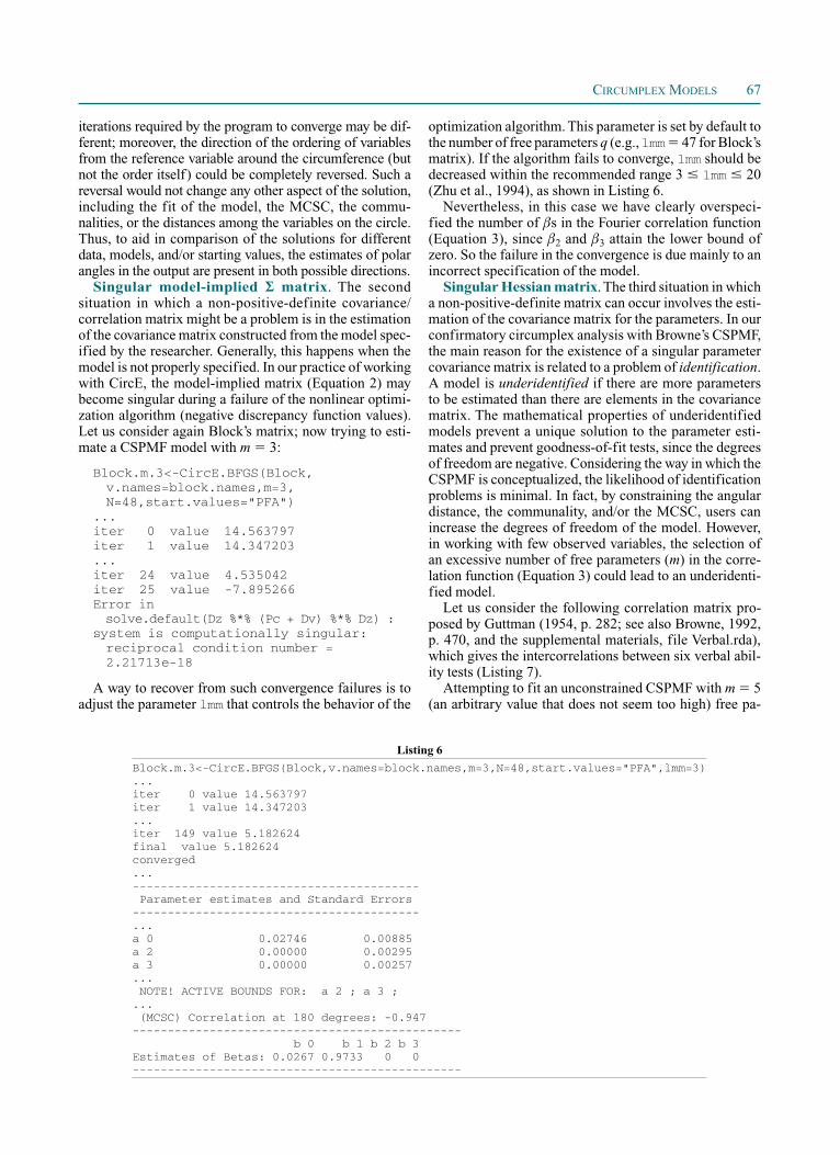
optimization algorithm. This parameter is set by default to the number of free parameters q (e.g., lmm 47 for Block’s matrix). If the algorithm fails to converge, lmm should be decreased within the recommended range 3 lmm 20 (Zhu et al., 1994), as shown in Listing 6.
Nevertheless, in this case we have clearly overspeci-fied the number of s in the Fourier correlation function (Equation 3), since 2 and 3 attain the lower bound of zero. So the failure in the convergence is due mainly to an incorrect specification of the model.
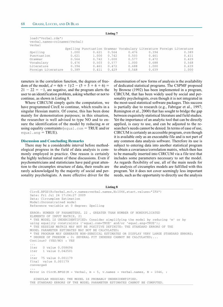
Singular Hessian matrix. The third situation in which a non-positive-definite matrix can occur involves the esti-mation of the covariance matrix for the parameters. In our confirmatory circumplex analysis with Browne’s CSPMF, the main reason for the existence of a singular parameter covariance matrix is related to a problem of identification. A model is underidentified if there are more parameters to be estimated than there are elements in the covariance matrix. The mathematical properties of underidentified models prevent a unique solution to the parameter esti-mates and prevent goodness-of-fit tests, since the degrees of freedom are negative. Considering the way in which the CSPMF is conceptualized, the likelihood of identification problems is minimal. In fact, by constraining the angular distance, the communality, and/or the MCSC, users can increase the degrees of freedom of the model. However, in working with few observed variables, the selection of an excessive number of free parameters (m) in the corre-lation function (Equation 3) could lead to an underidenti-fied model.
Let us consider the following correlation matrix pro-posed by Guttman (1954, p. 282; see also Browne, 1992, p. 470, and the supplemental materials, file Verbal.rda), which gives the intercorrelations between six verbal abil-ity tests (Listing 7).
Attempting to fit an unconstrained CSPMF with m 5 (an arbitrary value that does not seem too high) free pa-
iterations required by the program to converge may be dif-ferent; moreover, the direction of the ordering of variables from the reference variable around the circumference (but not the order itself) could be completely reversed. Such a reversal would not change any other aspect of the solution, including the fit of the model, the MCSC, the commu-nalities, or the distances among the variables on the circle. Thus, to aid in comparison of the solutions for different data, models, and/or starting values, the estimates of polar angles in the output are present in both possible directions.
Singular model-implied matrix. The second situation in which a non-positive-definite covariance/ correlation matrix might be a problem is in the estimation of the covariance matrix constructed from the model spec-ified by the researcher. Generally, this happens when the model is not properly specified. In our practice of working with CircE, the model-implied matrix (Equation 2) may become singular during a failure of the nonlinear optimi-zation algorithm (negative discrepancy function values). Let us consider again Block’s matrix; now trying to esti-mate a CSPMF model with m 3:
Block.m.3<-CircE.BFGS(Block, v.names=block.names,m=3, N=48,start.values="PFA")...iter 0 value 14.563797iter 1 value 14.347203...iter 24 value 4.535042iter 25 value -7.895266Error in solve.default(Dz %*% (Pc + Dv) %*% Dz) :system is computationally singular: reciprocal condition number = 2.21713e-18
A way to recover from such convergence failures is to adjust the parameter lmm that controls the behavior of the
Listing 6
Block.m.3<-CircE.BFGS(Block,v.names=block.names,m=3,N=48,start.values="PFA",lmm=3)...iter 0 value 14.563797iter 1 value 14.347203...iter 149 value 5.182624final value 5.182624converged... ----------------------------------------- Parameter estimates and Standard Errors-----------------------------------------...a 0 0.02746 0.00885a 2 0.00000 0.00295a 3 0.00000 0.00257... NOTE! ACTIVE BOUNDS FOR: a 2 ; a 3 ;... (MCSC) Correlation at 180 degrees: -0.947----------------------------------------------- b 0 b 1 b 2 b 3Estimates of Betas: 0.0267 0.9733 0 0-----------------------------------------------
68 GRASSI, LUCCIO, AND DI BLAS
dissemination of new forms of analysis is the availability of dedicated statistical programs. The CSPMF proposed by Browne (1992) has been implemented in a program, CIRCUM, that has been widely used by social and per-sonality psychologists, even though it is not integrated in the most-used statistical software packages. This success is partially due to research (e.g., Fabrigar et al., 1997; Remington et al., 2000) that has sought to bridge the gap between exquisitely statistical literature and field studies. Yet the importance of an analytic tool that can be directly applied, is easy to use, and can be adjusted to the re-searcher’s needs cannot be denied. In terms of ease of use, CIRCUM is certainly an accessible program, even though it is available only as an executable file and is not part of any common data analysis software. Therefore its use is subject to entering data into another statistical program to obtain a covariance/correlation matrix, which then has to be manually inserted into CIRCUM via a file text that includes some parameters necessary to set the model. As regards flexibility of use, all of the main needs for the analysis of circumplex models are fulfilled with this program. Yet it does not cover seemingly less important needs, such as the opportunity to directly use the analysis
rameters in the correlation function, the degrees of free-dom of the model, d 6(6 1)/2 (5 5 6 6) 21 22 1, are negative, and the program alerts the user to an identification problem, asking whether or not to continue, as shown in Listing 8.
Where CIRCUM simply quits the computation, we have programmed CircE to continue, which results in a singular Hessian matrix. Of course, this has been done mainly for demonstration purposes; in this situation, the researcher is well advised to type NO and to en-sure the identification of the model by reducing m or using equality constraints (equal.com TRUE and/or equal.ang TRUE).
Discussion and Concluding RemarksThere may be a considerable interval before method-
ological progress in the field of data analysis is com-monly employed in practice. One reason is certainly the highly technical nature of these discussions. Even if psychometricians and statisticians have paid great atten-tion to the circumplex structure of data, their results are rarely acknowledged by the majority of social and per-sonality psychologists. A more effective driver for the
Listing 7
load("Verbal.rda")verbal.names=colnames(Verbal)Verbal Spelling Punctuation Grammar Vocabulary Literature Foreign LiteratureSpelling 1.000 0.621 0.564 0.476 0.394 0.389Punctuation 0.621 1.000 0.742 0.503 0.461 0.411Grammar 0.564 0.742 1.000 0.577 0.472 0.429Vocabulary 0.476 0.503 0.577 1.000 0.688 0.548Literature 0.394 0.461 0.472 0.688 1.000 0.639Foreign Literature 0.389 0.411 0.429 0.548 0.639 1.000
Listing 8
CircE.BFGS(R=Verbal,m=5,v.names=verbal.names,N=1046,start.values="IFA")Date: Fri Jul 24 17:04:27 2009Data: Circumplex EstimationModel:Unconstrained modelReference variable at 0 degree: Spelling
ERROR: NUMBER OF PARAMETERS, 22 , GREATER THAN NUMBER OF NONDUPLICATEDELEMENTS OF INPUT MATRIX, 21* THE MODEL IS UNDERIDENTIFIED: Consider simplifying the model by reducing 'm' or byusing equality constraints ('equal.com=TRUE' and/or 'equal.ang=TRUE');* THE HESSIAN MATRIX MAY NOT BE POSITIVE DEFINITE: THE STANDARD ERRORS OF THEMODEL PARAMETER ESTIMATES MAY NOT BE CALCULATED;* THE PROGRAM MAY GENERATE NON-SENSICAL ESTIMATES OR DISPLAY VERY LARGE STANDARD ERRORS;* DEGREE OF FREEDOM < 0: SEVERAL FIT INDEXES CANNOT BE CALCULATED;...Continue? (YES/NO) : YES...iter 0 value 0.058694iter 1 value 0.042501...iter 75 value 0.001179final value 0.001179converged...Error in CircE.BFGS(R = Verbal, m = 5, v.names = verbal.names, N = 1046, :
SINGULAR HESSIAN: THE MODEL IS PROBABLY UNDERIDENTIFIED.THE STANDARD ERRORS OF THE MODEL PARAMETER ESTIMATES CANNOT BE COMPUTED.

CIRCUMPLEX MODELS 69
Block, J. (1957). Studies in the phenomenology of emotions. Journal of Abnormal & Social Psychology, 54, 358-363. doi:10.1037/h0040768
Bollen, K. A. (1989). Structural equations with latent variables. New York: Wiley.
Browne, M. W. (1982). Covariance structures. In D. M. Hawkins (Ed.), Topics in applied multivariate analysis (pp. 72-141). Cambridge: Cambridge University Press.
Browne, M. W. (1984). Asymptotically distribution-free methods for the analysis of covariance structures. British Journal of Mathematical & Statistical Psychology, 37, 62-83.
Browne, M. W. (1992). Circumplex models for correlation matrices. Psychometrika, 57, 469-497. doi:10.1007/BF02294416
Browne, M. W., & Cudeck, R. (1992). Alternative ways of assessing model fit. Sociological Methods & Research, 21, 230-258.
Browne, M. W., & Du Toit, S. H. C. (1992). Automated fitting of nonstandard models. Multivariate Behavioral Research, 27, 269-300. doi:10.1207/s15327906mbr2702_13
Byrd, R. H., Lu, P., Nocedal, J., & Zhu, C. (1995). A limited memory algorithm for bound constrained optimization. SIAM Journal on Sci-entific Computing, 16, 1190-1208. doi:10.1137/0916069
Di Blas, L., Grassi, M., Luccio, R., & Momentè, S. (2008). How children rate children: Structural continuity of the circumplex model of interpersonal behavior in late childhood. Manuscript submitted for publication.
Fabrigar, L. R., Visser, P. S., & Browne, M. W. (1997). Conceptual and methodological issues in testing the circumplex structure of data in personality and social psychology. Personality & Social Psychology Review, 1, 184-203. doi:10.1207/s15327957pspr0103_1
Fan, X., & Sivo, S. A. (2007). Sensitivity of fit indices to model mis-specification and model types. Multivariate Behavioral Research, 42, 509-529.
Guttman, L. (1954). A new approach to factor analysis: The radex. In P. F. Lazarsfeld (Ed.), Mathematical thinking in the social sciences (pp. 258-348). Glencoe, IL: Free Press.
Hu, L., & Bentler, P. M. (1999). Cutoff criteria for fit indexes in co-variance structure analysis: Conventional criteria versus new alterna-tives. Structural Equation Modeling, 6, 1-55.
Jöreskog, K. G. (1969). Efficient estimation in image factor analysis. Psychometrika, 34, 51-75. doi:10.1007/BF02290173
Liu, D. C., & Nocedal, J. (1989). On the limited memory BFGS method for large scale optimization. Mathematical Programming, 45, 503-528. doi:10.1007/BF01589116
MacCallum, R. C., Browne, M. W., & Sugawara, H. M. (1996). Power analysis and determination of sample size for covariance struc-ture modeling. Psychological Methods, 1, 130-149. doi:10.1037/1082 -989X.1.2.130
R Core Team Members, DebRoy, S., Bivand, R., et al. (2008). for-eign: Read data stored by Minitab, S, SAS, SPSS, Stata, Systat, dBase, . . . (R package version 0.8-26). Vienna: R Foundation for Statistical Computing.
R Development Core Team (2008). R: A language and environment for statistical computing (ISBN 3-900051-07-0). Vienna: R Founda-tion for Statistical Computing.
Remington, N. A., Fabrigar, L. R., & Visser, P. S. (2000). Reexamin-ing the circumplex model of affect. Journal of Personality & Social Psychology, 79, 286-300. doi:10.1037/0022-3514.79.2.286
Schumacker, R. E., & Lomax, R. G. (1996). A beginner’s guide to structural equation modeling. Mahwah, NJ: Erlbaum.
Shapiro, A. (1985). Asymptotic distribution of test statistic in the analy-sis of moment structures under inequality constraints. Biometrika, 72, 133-144. doi:10.1093/biomet/72.1.133
Shapiro, A. (1989). Asymptotic properties of statistical estimators in stochastic programming. Annals of Statistics, 17, 841-858. Available at http://projecteuclid.org/euclid.aos/1176347146.
SPSS Inc. (1999). SPSS base 10.0 for Windows user’s guide. Chicago: Author.
Steiger, J. H., & Lind, J. M. (1980, June). Statistically based tests for the number of common factors. Paper presented at the annual meeting of the Psychometric Society, Iowa City, IA.
Wiggins, J. S. (1979). A psychological taxonomy of trait-descriptive terms: The interpersonal domain. Journal of Personality & Social Psy-chology, 37, 395-412. doi:10.1037/0022-3514.37.3.395
results for further processing. Indeed, graphical repre-sentations of variables along the circumference and of the estimated FS correlation function must be produced by external software, into which the necessary informa-tion must be entered to obtain the graphs. The quality of the final result is then directly proportional to the user’s ability to stray from the default graphical settings of the software used.
Although these are minor problems if CIRCUM is used only occasionally, exploratory analyses, above all in terms of questionnaire items, would be much simplified if (1) the statistical routine were integrated in the software used for data entry, (2) the results of the analysis could be represented in a graph, and (3) the chance to constrain the estimates could be extended to items that are conceptually linked to higher-order variables, in order to assess the em-pirical tenability of their expected circular organization. In the present article, we have presented an R package for fit-ting circumplex models, an alternative to the widely used CIRCUM. It is “alternative” in the senses that the results provided by CircE are convergent with those obtained by CIRCUM and that the options for constraining the model allowed by CIRCUM are present also in CircE. Moreover, CircE has the compelling advantages of being integrated in one of the most widely used packages for statistical computing and of providing users with graphical func-tions, as well as providing users with the ability to specify bounded estimations of polar angles, which is particularly appropriate in questionnaire item analysis. As seen in the child interpersonal circumplex example, each item can be constrained to fall within a specific 45º arc; that is, items are constrained to be distributed across the eight octants LM to JK, which cover the whole circumference and rep-resent different possible DOM/LOV combinations. This approach allows testing of whether an expected organiza-tion of items into scales is empirically robust, whereas other presently available statistical packages do not allow for testing such specific circular distributions of an item. All of these features are programmed in an open language that is easy to check and modify with minor programming effort. A future enhancement would be to expand CircE’s computational capabilities to multiple-group models and alternative fitting functions, such as the asymptotically distribution-free discrepancy function (Browne, 1984; Yung & Bentler, 1994). The rapidity with which this will be accomplished will depend on users’ interest.
AUTHOR NOTE
We thank Michael W. Browne for useful documentation he provided and Michael Siegal for comments on an earlier draft. We also thank the three anonymous reviewers, who helped us improve this article. Cor-respondence concerning this article should be addressed to M. Grassi, Department of Psychology “G. Kanizsa,” Via Sant’ Anastasio 12, 34134, Trieste, Italy (e-mail: [email protected]).
REFERENCES
Anderson, T. W. (1960). Some stochastic process models for intelli-gence test scores. In K. J. Arrow, S. Karlin, & P. Suppes (Eds.), Mathe-matical methods in the social sciences, 1959 (pp. 205-220). Stanford: Stanford University Press.

70 GRASSI, LUCCIO, AND DI BLAS
5. In addition to the stopping test in Equation 6, the algorithm has an-other built-in stopping test based on the projected gradient: The iteration will stop when max{ | proj gi | (i 1, . . . , q)} pgtol; the user can sup-press this termination test by setting pgtol 0. By default, this termina-tion test is suppressed because L-BFGS-B is sometimes unable to reduce the projected gradient sufficiently to satisfy the stopping condition, even though the function value obtained is very good (Zhu et al., 1994).
6. Netlib is a repository of software for scientific computing main-tained by AT&T, Bell Laboratories, the University of Tennessee, and Oak Ridge National Laboratory.
7. The initial estimates of parameters k provided by the factor anal-ysis method are used to obtain the initial estimates k k / 1, with
1 1 held fixed during the optimization process.8. A fourth message may refer to the asymptotic covariance matrix.
This is not the covariance matrix being analyzed, but rather a weight ma-trix to be used with asymptotically distribution-free estimation (Browne, 1984; Yung & Bentler, 1994) that is not yet implemented in both the CIRCUM and CircE programs.
SUPPLEMENTAL MATERIALS
The CircE package (for Mac OS X or Windows), as well as R source code and the example files discussed in the text, may be downloaded from http://brm.psychonomic-journals.org/content/supplemental.
Wiggins, J. S., & Trapnell, P. D. (1996). A dyadic–interactional per-spective on the five-factor model. In J. S. Wiggins (Ed.), The five-factor model of personality: Theoretical perspectives (pp. 88-162). New York: Guilford.
Wothke, W. (1993). Nonpositive definite matrices in structural model-ing. In K. A. Bollen & J. S. Long (Eds.), Testing structural equation models (pp. 256-293). Newbury Park, CA: Sage.
Yung, Y.-F., & Bentler, P. M. (1994). Bootstrap-corrected ADF test statistics in covariance structure analysis. British Journal of Math-ematical & Statistical Psychology, 47, 63-84.
Zhu, C., Byrd, R., Lu, P., & Nocedal, J. (1994, December). L-BFGS-B: Fortran subroutines for large-scale bound constrained optimiza-tion (Rep. NAM-11). Evanston, IL: Northwestern University, EECS Department.
NOTES
1. Like other covariance structure models, Browne’s model assumes that variance in people’s responses can be divided into the common score variance and the unique score variance.
2. That is, the correlation between common score variables that are 180º apart from one another on the circle.
3. www.R-project.org.4. That is, users are free to use, modify, and distribute the program.
APPENDIX A CircE Output
Unconstrained CSPMF, With m 1, for the Correlation Matrix in Table 1Voc.unconstr<-CircE.BFGS(R=R.vocational,v.names=v.names,m=1,N=175,equal.com=FALSE, equal.ang=FALSE,mcsc="unconstrained",iterlim=250,factr=1e06)
Date: Tue Jun 30 09:49:33 2009Data: Circumplex EstimationModel:Unconstrained modelReference variable at 0 degree: Health
Constrained (L-BFGS-B) Optimizationiter 0 value 0.191801iter 1 value 0.164363iter 2 value 0.134711iter 3 value 0.120156iter 4 value 0.105840...iter 43 value 0.089815iter 44 value 0.089815iter 45 value 0.089815final value 0.089815converged
============================= MEASURES OF FIT OF THE MODEL =============================
-----------Sample discrepancy function value : 0.09
-----------Population discrepancy function value, Fo Point estimate : 0.049 Confidence Interval 90 % : ( 0.005 ; 0.139 )
-----------ROOT MEAN SQUARE ERROR OF APPROXIMATION Steiger-Lind: RMSEA=sqrt(Fo/Df) Point estimate : 0.084 Confidence Interval 90 % : ( 0.026 ; 0.141 )
-----------Discrepancy function TEST TEST STATISTIC : 15.63 p values: Ho: perfect fit (RMSEA=0.00) : 0.029 Ho: close fit (RMSEA=0.050) : 0.137

CIRCUMPLEX MODELS 71
-----------Power estimation (alpha=0.05), N 175 Degrees of freedom= 7 Effective number of parameters= 21 Ho (RMSEA=0.05) vs Alternative (RMSEA=0.01) : 0.135 Ho (RMSEA=0.05) vs Alternative (RMSEA=0.06) : 0.085 Ho (RMSEA=0.05) vs Alternative (RMSEA=0.08) : 0.215 Ho (RMSEA=0.00) vs Alternative (RMSEA=0.05) : 0.195
-----------EXPECTED CROSS VALIDATION INDEX Browne and Cudeck’s Index BCI-(MODIFIED AIC) Point estimate : 0.343 Confidence Interval 90 % : ( 0.298 ; 0.432 )
Hoelter’s CN( .05 ) : 154
-----------Fit index Chisquare (null model) = 747.663 Df = 21 Bentler-Bonnett NFI : 0.979 Tucker-Lewis NNFI : 0.964 Bentler CFI : 0.988 SRMR : 0.04 GFI : 0.986 AGFI : 0.944-----------Parsimony index Akaike Information Criterion : -0.152 Bozdogans’s Consistent AIC : -113.833 Schwarz’s Bayesian Criterion : -0.534
---------------------------------------- Parameter estimates and Standard Errors---------------------------------------- Parameters Stand. ErrorsHealth 0.00000 0.00000Science 305.35328 9.01111Technology 247.82980 7.35838Trades 237.38218 9.44904Business Operations 168.30615 9.08050Business Contact 149.83787 7.95016Social 91.25973 8.72929a 0 1.76119 0.26287v Health 0.15438 0.13759v Science 0.51654 0.12755v Technology 0.03945 0.04238v Trades 0.63153 0.13854v Business Operations 0.54550 0.12125v Business Contact 0.13449 0.05959v Social 0.44771 0.13865z Health 0.91358 0.07570z Science 0.81222 0.06530z Technology 1.00102 0.05839z Trades 0.79058 0.06533z Business Operations 0.79269 0.06325z Business Contact 0.92497 0.05923z Social 0.84376 0.06916
--------------------------------------------------------------------------- Estimates (ML) of POLAR ANGLES and COMMUNALITY INDICES (approximate 95% one at time confidence intervals) Note: variable names have been reordered to yield increasing polar angles--------------------------------------------------------------------------- ang. pos. (L ; U) 360-ang. pos. (L ; U) comm. ind. (L ; U)Health 0 ( 0 ; 0 ) 360 ( 360 ; 360 ) 0.93 ( 0.73 ; 0.99 )Social 91 ( 74 ; 108 ) 269 ( 286 ; 252 ) 0.83 ( 0.74 ; 0.9 )Business Contact 150 ( 134 ; 165 ) 210 ( 226 ; 195 ) 0.94 ( 0.87 ; 0.97 )Business Operations 168 ( 151 ; 186 ) 192 ( 209 ; 174 ) 0.80 ( 0.74 ; 0.86 )Trades 237 ( 219 ; 256 ) 123 ( 141 ; 104 ) 0.78 ( 0.71 ; 0.84 )Technology 248 ( 233 ; 262 ) 112 ( 127 ; 98 ) 0.98 ( 0.87 ; 1 )Science 305 ( 288 ; 323 ) 55 ( 72 ; 37 ) 0.81 ( 0.74 ; 0.87 )
APPENDIX A (Continued)
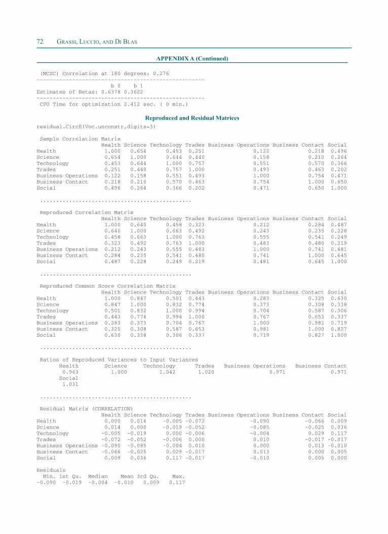
72 GRASSI, LUCCIO, AND DI BLAS
APPENDIX A (Continued)
(MCSC) Correlation at 180 degrees: 0.276---------------------------------------------------- b 0 b 1Estimates of Betas: 0.6378 0.3622---------------------------------------------------- CPU Time for optimization 2.412 sec. ( 0 min.)
Reproduced and Residual Matricesresidual.CircE(Voc.unconstr,digits=3)
Sample Correlation Matrix Health Science Technology Trades Business Operations Business Contact SocialHealth 1.000 0.654 0.453 0.251 0.122 0.218 0.496Science 0.654 1.000 0.644 0.440 0.158 0.210 0.264Technology 0.453 0.644 1.000 0.757 0.551 0.570 0.366Trades 0.251 0.440 0.757 1.000 0.493 0.463 0.202Business Operations 0.122 0.158 0.551 0.493 1.000 0.754 0.471Business Contact 0.218 0.210 0.570 0.463 0.754 1.000 0.650Social 0.496 0.264 0.366 0.202 0.471 0.650 1.000
...............................................
Reproduced Correlation Matrix Health Science Technology Trades Business Operations Business Contact SocialHealth 1.000 0.640 0.458 0.323 0.212 0.284 0.487Science 0.640 1.000 0.663 0.492 0.243 0.235 0.228Technology 0.458 0.663 1.000 0.763 0.555 0.541 0.249Trades 0.323 0.492 0.763 1.000 0.483 0.480 0.219Business Operations 0.212 0.243 0.555 0.483 1.000 0.741 0.481Business Contact 0.284 0.235 0.541 0.480 0.741 1.000 0.645Social 0.487 0.228 0.249 0.219 0.481 0.645 1.000
...............................................
Reproduced Common Score Correlation Matrix Health Science Technology Trades Business Operations Business Contact SocialHealth 1.000 0.847 0.501 0.443 0.283 0.325 0.630Science 0.847 1.000 0.832 0.774 0.373 0.308 0.338Technology 0.501 0.832 1.000 0.994 0.704 0.587 0.306Trades 0.443 0.774 0.994 1.000 0.767 0.653 0.337Business Operations 0.283 0.373 0.704 0.767 1.000 0.981 0.719Business Contact 0.325 0.308 0.587 0.653 0.981 1.000 0.827Social 0.630 0.338 0.306 0.337 0.719 0.827 1.000
...............................................
Ratios of Reproduced Variances to Input Variances Health Science Technology Trades Business Operations Business Contact 0.963 1.000 1.042 1.020 0.971 0.971 Social 1.031
...............................................
Residual Matrix (CORRELATION) Health Science Technology Trades Business Operations Business Contact SocialHealth 0.000 0.014 -0.005 -0.072 -0.090 -0.066 0.009Science 0.014 0.000 -0.019 -0.052 -0.085 -0.025 0.036Technology -0.005 -0.019 0.000 -0.006 -0.004 0.029 0.117Trades -0.072 -0.052 -0.006 0.000 0.010 -0.017 -0.017Business Operations -0.090 -0.085 -0.004 0.010 0.000 0.013 -0.010Business Contact -0.066 -0.025 0.029 -0.017 0.013 0.000 0.005Social 0.009 0.036 0.117 -0.017 -0.010 0.005 0.000
Residuals Min. 1st Qu. Median Mean 3rd Qu. Max.-0.090 -0.019 -0.004 -0.010 0.009 0.117
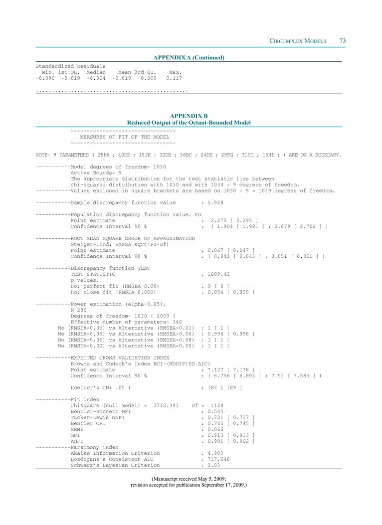
CIRCUMPLEX MODELS 73
APPENDIX B Reduced Output of the Octant-Bounded Model
================================= MEASURES OF FIT OF THE MODEL =================================
NOTE: 9 PARAMETERS ( 28PA ; 40DE ; 19JK ; 32DE ; 38BC ; 24DE ; 29FG ; 31HI ; 15HI ; ) ARE ON A BOUNDARY.
-----------Model degrees of freedom= 1030 Active Bounds= 9 The appropriate distribution for the test statistic lies between chi-squared distribution with 1030 and with 1030 + 9 degrees of freedom.-----------Values enclosed in square brackets are based on 1030 + 9 = 1039 degrees of freedom.
-----------Sample discrepancy function value : 5.928
-----------Population discrepancy function value, Fo Point estimate : 2.275 [ 2.295 ] Confidence Interval 90 % : ( 1.904 [ 1.921 ] ; 2.679 [ 2.702 ] )
-----------ROOT MEAN SQUARE ERROR OF APPROXIMATION Steiger-Lind: RMSEA=sqrt(Fo/Df) Point estimate : 0.047 [ 0.047 ] Confidence Interval 90 % : ( 0.043 [ 0.043 ] ; 0.051 [ 0.051 ] )
-----------Discrepancy function TEST TEST STATISTIC : 1689.42 p values: Ho: perfect fit (RMSEA=0.00) : 0 [ 0 ] Ho: close fit (RMSEA=0.050) : 0.854 [ 0.899 ]
-----------Power estimation (alpha=0.05), N 286 Degrees of freedom= 1030 [ 1039 ] Effective number of parameters= 146 Ho (RMSEA=0.05) vs Alternative (RMSEA=0.01) : 1 [ 1 ] Ho (RMSEA=0.05) vs Alternative (RMSEA=0.06) : 0.996 [ 0.996 ] Ho (RMSEA=0.05) vs Alternative (RMSEA=0.08) : 1 [ 1 ] Ho (RMSEA=0.00) vs Alternative (RMSEA=0.05) : 1 [ 1 ]
-----------EXPECTED CROSS VALIDATION INDEX Browne and Cudeck’s Index BCI-(MODIFIED AIC) Point estimate : 7.127 [ 7.178 ] Confidence Interval 90 % : ( 6.756 [ 6.804 ] ; 7.53 [ 7.585 ] )
Hoelter’s CN( .05 ) : 187 [ 189 ]
-----------Fit index Chisquare (null model) = 3712.393 Df = 1128 Bentler-Bonnett NFI : 0.545 Tucker-Lewis NNFI : 0.721 [ 0.727 ] Bentler CFI : 0.745 [ 0.745 ] SRMR : 0.066 GFI : 0.913 [ 0.913 ] AGFI : 0.901 [ 0.902 ]-----------Parsimony index Akaike Information Criterion : 4.903 Bozdogans’s Consistent AIC : 717.648 Schwarz’s Bayesian Criterion : 3.03
(Manuscript received May 5, 2009; revision accepted for publication September 17, 2009.)
Standardized Residuals Min. 1st Qu. Median Mean 3rd Qu. Max.-0.090 -0.019 -0.004 -0.010 0.009 0.117
................................................
APPENDIX A (Continued)