Embed Size (px)
Citation preview

Trakya Üniversitesi Mühendislik Bilimleri Dergisi
Cilt: 13 Sayı: 2 Aralık 2012
Trakya UniversiTy JoUrnal of engineering sciences
Volume: 13 Number: 2 December 2012 Trakya Univ J Eng Sci
http://fbe.trakya.edu.tr/tujes e-mail: [email protected]
ISSN 2147 0308

Trakya Üniversitesi Mühendislik Bilimleri Dergisi
Cilt: 13 Sayı: 2 Aralık 2012
Trakya University Journal of Engineering Science
Volume: 13 Number: 2 December 2012
Trakya Univ J Eng Sci
http://fbe.trakya.edu.tr/tujes e-mail: [email protected]
ISSN 2147 0308

Trakya Üniversitesi Mühendislik Bilimleri Dergisi http://fbe.trakya.edu.tr/tujes Cilt 13 Sayı 2, Aralık 2012
ISSN 2147 0308 Trakya Univ Journal of Engineering Sciencei Volume 13 Number2, December 2012
Dergi Sahibi / Owner
Trakya Üniversitesi Rektörlüğü Fen Bilimleri Enstitüsü Adına On behalf of Trakya University Rectorship, Graduate School of Natural and Applied Sciences Prof. Dr. Mustafa ÖZCAN Editör / Editor Prof .Dr. Metin AYDOĞDU Yardımcı Editör / Associate Editor Y.Doç. Dr. Deniz AĞIRSEVEN Dergi Yayın Kurulu / Editorial Board Başkan / Chairman Prof. Dr. Mustafa ÖZCAN Üyeler / Members Prof.Dr. Metin AYDOĞDU Y.Doç.Dr. Deniz AĞIRSEVEN Prof.Dr. Taner TIMARCI Y.Doç. Dr. Derya ARDA Y.Doç.Dr. Oğuzhan ERDEM Dizgi / Design Recep KARA, [email protected] Prof.Dr.Metin AYDOĞDU, [email protected] Yazışma Adresi / Correspondence Address T rakya Üniversitesi Fen Bilimleri Enstitüsü Binası, Balkan Yerleşkesi – 22030 Edirne / TÜRKİYE e-mail:[email protected] Tel: +90 284 2358230 Fax: +90 284 2358237 Baskı / Publisher Trakya Üniversitesi Matbaa Tesisleri / Trakya University Publishing Centre

Trakya University Journal of Engineering Science Danışma Kurulu / Advisory Board
Ahmet PINARBAŞI, Çukurova Üniversitesi, ADANA
Asım KURTOĞLU, Royal Institue of Technol,SWEDEN
Ayşegül AKDOĞAN EKER, Yıldız Teknik Üniversitesi,İSTANBUL
Burhan ÇUHADAROĞLU, Karadeniz Teknik Üniversitesi, TRABZON
Bülent DOYUM, Orta Doğu Teknik Üniversitesi, ANKARA
Erhan AKIN, Fırat Üniversitesi, ELAZIĞ
Erhan COŞKUN, Karadeniz Teknik Üniversitesi,TRABZON
Fahri YAVUZ, Atatürk Üniversitesi,ERZURUM
H.Avni CİNEMRE,Ondokuz Mayıs Üniversitesi, SAMSUN
İsmail H. TAVMAN,Dokuz Eylül Üniversitesi,İZMİR
Kadir KIRKKÖPRÜ, İstanbul Teknik Üniversitesi,İSTANBUL
Kai CHENG, Brunel University,Uxbridge,West London,UK
Mehmet Baki KARAMIŞ,Erciyes Üniversitesi,KAYSERİ
Mehmet BOZOĞLU,Ondokuz Mayıs Üniversitesi,SAMSUN
Mehmet KOPAÇ,Zonguldak Karaelmas Üniversitesi,ZONGULDAK
Nadia ERDOĞAN,İstanbul Teknik Üniversitesi,İSTANBUL
Narayana BALASUBRAMANIAN,Center for the Study of Science,Bangalore,INDIA
Şazuman SAZAK,Trakya Üniversitesi,EDİRNE
Tülay YILDIRIM,Yıldız Teknik Üniversitesi,İSTANBUL
Türkan Göksal ÖZBALTA,Ege Üniversitesi,İZMİR
Visvalingam BALASUBRAMANIAN, Annamalai University,CEMAJOR, Nagar, INDIA

Trakya Üniversitesi Mühendislik Bilimleri Dergisi http://fbe.trakya.edu.tr/tujes Cilt 13 Sayı 2, Aralık 2012
ISSN 2147 0308 Trakya Univ Journal of Engineering Sciencei Volume 13 Number2, December 2012
İÇİNDEKİLER / CONTENTS Behavior of Biaxially Loaded Concrete Columns under Fire Exposure Ataman HAKSEVER 73-87 Maximizing Tensile Strength and Minimizing Interface Hardness of Friction Welded Dissimilar Joints of Austenitic Stainless Steel and Aluminium Alloy G.Vairamani, T.Senthil Kumar, S.Malarvizhi and V.Balasubramanian 89-107 A Web-Control Based Student Classroom Attendence Tracking System Application: TUODS Deniz Mertkan GEZGİN 109-119 3D Modellemede Kullanılan Ardışık Yansıtmalı Yapılandırılmış Işık Yöntemleri Eser SERT, Deniz TAŞKIN, Olcay ÖZCAN, Cem TAŞKIN, Kenan BAYSAL 121-141
VHDL Kullanılarak FPGA İle Yüksek Kapasitel, Toplayıcı Ünite Tasarımı
Deniz TAŞKIN, Kenan BAYSAL, Eser SERT, Cem TAŞKIN, Murat Olcay ÖZCAN
143-156

http://fbe.trakya.edu.tr/tujs Trakya Univ J Sci, 13(2): 73-87, 2012 ISSN 2147–0308 DIC: 003AHTT1321204130413
BEHAVIOR OF BIAXIALLY LOADED CONCRETE COLUMNS UNDER FIRE
EXPOSURE
Ataman HAKSEVER Department of Civil Engineering, Namık Kemal University, Tekirdağ,TURKEY
ÖZET
Eğik eğilmeye maruz betonarme kolonların yangın dayanımı, karmaşık bir hesap işlemi gerktirmektedir. Burada tanıtılacak olan bir yöntem ile yangın durumu için betonarme kolonların eğik eğilme problemi, tek eksenli dayanım hesabına indirgenmektedir.
ABSTRACT
This paper aims at developing a simplified calculational method to be used to
determine the behavior of biaxial loaded reinforced concrete columns in fire. By aid of a developed calculation method, which uses the superpositon principle, the uniaxial bending of reinforced concrete columns has been analyzed.
Keywords: Fire, reinforced concrete columns, fire resistance, numerical modelling,
fire design, Eurocode 2, thermal curvature.
1.INTRODUCTION
Fire is one of the serious potential risks to most buildings and structures. The extensive use of concrete as a structural material has led to the need to understand the effects of fire on reinforced concrete structures. Generally, concrete is known to have good fire resistance.
Reinforced concrete columns are predominantly stressed by the comp-ression forces.
They are in buildings connected to other structural members, like beams, girders and slabs. If a building or part of it is exposed to a local fire, the reinforced concrete columns experience in addition to direct thermal and mechanical stress attacks also loadings due to uneven thermal deformation of surrounding structures /1-3/. Gradually the strength reduction in materials, cracking, spalling of individual concrete regions yielding of steel reinforcement as well will result in complete different statical systems due to plastic hinges in statically indeterminate structures /4/.
To build up a model to analyse these effects, an extensive investigation of reinforced
concrete columns was carried out at the special fire research department of the Technical University Braunschweig (SFB 1481) /5, 6/. In this paper, the behavior of biaxially loaded concrete columns is analyzed as a part of this project and a simplified calculation method is developed for the fire case.
1 Sonderforschungsbereich 148, a special research project for investigation of fire behavior of structural systems
Araştırma Makalesi / Research Article

74 Ataman HAKSEVER
Trakya Univ J Eng Sci, 13(2), 73-87, 2012
1.BIAXIALLY LOADED REINFORCED CONCRETE COLUMNS UNDER FIRE EXPOSUREL
Due to the uneven temperature distribution and the behavior of the neighboring struc-
tures, the cross-sections of the column will take rather large deformations, and they do not remain as plane in the deformation any more. However in the method developed, the pre-sumption about retaining the planar, but biaxial inclined cross-section is adopted. This load-ing corresponds to three-dimensional beam bending with biaxial deformation. In figure 2.1, the deformed geometry and the applied loads are illustrated /9/. The deformed shape of the cross-section will take on the base of the presumptions a form of an oblique plane. The beam buckling with bending corresponds to a possible collapse of the column. The possible loading conditions for a reinforced concrete column in case of fire in which a biaxial deformation shape can take place are indicated below.
-THREE DIMENSIONAL END DEFORMATIONS
-NONUNIFORM HEATING OF THE CROSS-SECTION -TWO-DIMENSIONAL BENDING CASE
Due to a nonsymmetric heat-ing of the cross-section, the develop-ing expansions will
cause directly a biaxial bending of the concrete column. On the other hand, if the acting bending moments result in stress condition which may not coincide with the both main axes y and z, a biaxial deformation will follow due to the non-uniform ex-pansions additionally. These defor-mation conditions can also appear in different combinations. However, this paper will take into account only the bending moments which cause a biaxial bending situation under sym-metrical heating. Figure 2.2 shows the warping of the cross-section in case of biaxial bending.
This paper aims at developing simplified calculational method to be used in iterative computation in order to determine the behavior of biaxial loaded reinforced concrete columns in fire and verify the calculation results by means of the test results.
Fig. 2.1: Statical System /9/

BEHAVIOR OF BIAXIALLY LOADED CONCRETE COLUMNS 75
3.MATERIAL PROPERTIES AND THE DIMENSIONS OF THE TEST SPECIMENS
Six fire tests with concrete columns were carried out in order to investigate the loss of
stiffness under fire attack and loading conditions /9/. In SFB148 mainly, the uniaxially loaded columns were investigated under fire action. In the tests, a uniform heating of the column was maintained from all sides which rendered the possibility that the bending took place in the loading plane. These tests did not consider how-ever that the deformation of the columns can be restricted by surrounding structures, yielding biaxial bending deformations. The bearing and deformation behavior of such columns can be substantially determined by the bending rigidities of the cross-section in
main directions /9, 10/. In Table 3.1, the geometry and the dimensions of the specimens are presented, whilst Table 3.2 gives information about the material properties of the specimens (s. also Fig. 3.1).
Table 3.1: Geometry and the dimensions of specimens /9/
Fig. 2. 2: Biaxial bending plane for a 30/30 cross- section in fire case

76 Ataman HAKSEVER
Trakya Univ J Eng Sci, 13(2), 73-87, 2012
Experimental and theoretical research covered systematic tests which were performed for biaxially loaded concrete columns in SFB148 /9, 10/. The temperatures in the furnace were controlled with respect to the ISO 834 temperature curve. In contrary to the uniaxial loaded columns, the boundary conditions were constructed to be three-dimensional hinges at each end, so that the correspondence to Euler Case II for beam buckling was reached. The loading regions at the column ends were protected carefully against the thermal loading.
Table 3.2: Material properties of the specimens /9/
Fig. 3.1. Geometry of the specimens and location of the reinforcements /9, 10/

BEHAVIOR OF BIAXIALLY LOADED CONCRETE COLUMNS 77
The bending stiffnesses of the cross-section chosen deviate obviously from each other. The slendernesses in two main directions are 51 and 102, respectively /9, 10/. The reinforcement bars are distributed uniformly along the sides of the cross-section. The systematic axial loads applied in the tests were in many cases somewhat lower than the design loads for room temperatures. Despite this fact, no specimen attained the fire resistance of an hour, though the columns satisfied the regulations of DIN 4102. In figure 3.1 the geometry and the location of the reinforcing of the specimens are illustrated.
4.CALCULATION METHOD 4.1 Assumptions In order to determine the fire behavior of concrete columns under fire attack in case of
biaxial loading, a simple calculation method has been developed. It is based on the uniaxial stress distribution. The calculation method takes into account the following assumptions:
1. At each time step, at which the stability analysis will be carried out, the
temperature distribution over the cross-section remains unchanged.
2. Beam theory is applied, shear stresses are neglected.
3. Cross-sections retain their planes in the deformation. Torsion and shear effects will not be taken into account.
4. Applied loads remain constant during the fire.
5. Local effects are excluded.
6. The temperature bound thermal properties of the material are taken into
account with time effects .
7. The stability analysis is carried out according to the second order theory.
Load bearing capacity and deformation behavior of concrete columns in fire are mainly influenced by nonsteady temperature distribution. The deter-mination or the temperature fields in these members is therefore the primary assumption for the further computational treatment of the fire problem except that the temperature distributions were obtained by means of experiments prior to calculations /5, 6, 11/.
4.2 Nonsteady temperature developments in cross-sections The mathematical treatment of the non-steady temperature problem was first carried
out by J. R. Fourier in 1822. The general heat transfer equation named after him has the form:
])[(.).( TgradTdivtTTc p λρ =∂∂ +W (4.1)

78 Ataman HAKSEVER
Trakya Univ J Eng Sci, 13(2), 73-87, 2012
The development of efficient computers now allows more realistic solutions by the use of numerical techniques. The term T(t) is the temperature distribution in a cross-section which has to be considered as an additional unknown parameter, while λ(T) shows the thermal conductivity, cp(T) indicates specific heat capacity of the concrete material. Because there is no heat source in the column the internal heat source W is set to zero. The solution of the Eq. 4.1 is obtained from the consideration of one-dimensional heat transfer conditions. It is accepted that the heat transfer along the column axis to be uniform. The mathematical treatment of this equation is discussed in the relevant literature /3, 11/. For this purpose, the cross-section is divided into surface elements by a net-like system.
4.3 Determination of the deflections Several methods are available for the determination of displacements and the the slope
at each point on the column axis. A numerical solution of the differential equation for deflection can be obtained by finite differences. Calculation of the deformations is carried out at equidistant nodes of the column by applying elastic weights iw at the nodes as concentrated loading with respect to the equation Eq. 4.2.
It can be shown that the moment iM at any nodal point of the conjugate column due to the elastic weights is equal to the deflection y at the corresponding point in the actual column. The elastic weights are calculated by Eq. 4.2.
(4.2) ∫∫ +=ll
rrr
ll
i dxxdxxwλλ
κλ
κλ 0
20
11
11
Fig. 4.1: Elastic weights for the calculation of the y deflections

BEHAVIOR OF BIAXIALLY LOADED CONCRETE COLUMNS 79
Figure 4.1 shows schematically three successive nodal points i-1, i, i+1 in a column
subjected to irregular loading along the x-axis. These points will be referred to as nodes. The curvature κ must be determined with respect to the biaxial bending, which means that strains at three separate points of the cross-section must be determined (s. Figs. 2.2, 4.3).
4.4 Calculation of the warping of the cross-sections The non-linear warping of a cross-section is related to the acting internal forces and
temperature distribution. It can be expressed by the Eq. (4.1)
κP,T = κP,T (M, N, T) (4.1)
The curvature function κP,T is generally nonlinear and can be determined iteratively by numerical procedures which can give sufficient accuracy. In this case, the curvature of the beam axis is dependent on the bending moment, applied axial load and actual temperature distribution on the cross-section plane. The curvature κ of the beam under applied loads and the fire action can be written in Eq. (4.2) for an uniaxial bending as
(4.2)
In figure 4.2, the thermal expansion εth and the deformed cross-section plane are
illustrated in the equilibrium condition of a cross-section. εr represents the cracked area in concrete while εth is the thermal expansion and εt shows the total strain on the Bernoulli-Plane. Figure 4.2 shows that the thermal expansion is naturally not uniform on the cross-section plane. Restrained areas and the strains which cause the internal stress distribution are hatched on the picture. Stress calculation considers the nonlinear material behavior σ=σ(εr,T) related to the acting temperature and stress history.
The acting internal forces are dependant on the edge strains ε1, ε2 and can be written as
given in Eq. (4.3).
Fig. 4.2: Deformation and equilibr- ium condition of a cross section in case of fire for uniaxial bending /3/.
hTP21
,εεκ −
=

80 Ataman HAKSEVER
Trakya Univ J Eng Sci, 13(2), 73-87, 2012
),( 211 εεfN = ),( 212 εεfM = (4.3)
In case of biaxial bending Eq. (4.3) becomes a more complex expression as shown in
Eq. (4.4).
),,(1 cbafN = ),,(2 cbafM y = ),,(3 cbafM z = (4.4) The strains of the nodal element a, b, c can be determined iteratively by the solution of
the total differentials of the simultaneous functions in Eq. (4.5)
NccNb
bNa
aN
∆=∆+∆+∆δδ
δδ
δδ (4.5.1)
zzzz Mc
cM
bb
Ma
aM
∆=∆+∆+∆δδ
δδ
δδ
(4.5.2)
yyyy Mc
cM
bb
Ma
aM
∆=∆+∆+∆δδ
δδ
δδ
(4.5.2)
The ΔN, ΔMz and ΔMy values indicate the differ-ences between the calculation and the external forces at the nodal point at each iteration step while a, b, c are the coordinates of the biaxial plane as strains (s. Fig. 4.3), by which the plane equation can be written as given by the Eq. (4.6).
1=++az
by
cx
(4.6)
The iterations must be set simultaneously so the equations (4.7) are suffi-ciently verified:
0),,(11 →−=∆ ++ iii NcbaNN (4.7.1)
0),,( ,1,1,, →−=∆ ++ iziziz McbaMM (4.7.2) 0),,( ,1,1, →−=∆ ++ iyiyiyz McbaMM (4.7.3)
Fig. 4.3: Coordinates of the biaxial plane

BEHAVIOR OF BIAXIALLY LOADED CONCRETE COLUMNS 81
The coordinates a, b and c can be improved at each iteration step i in Eq. (4.8) by the correction values Δa, Δb and Δc
11 ++ ∆+= iii aaa (4.8)
Similar equations can be written also for b and c. However, the simultaneous solution of those parameters becomes rather laborious and even the computer application is time consuming. In order to simplify the calculation, a method is developed here which uses the regulations in DIN 1045 /7, 8/ and it is verified with the tests in SFB148. In DIN 1045, it is shown that the biaxial bending design of reinforced concrete columns can be transferred to the uniaxial bending case if certain conditions are present. This regulation in DIN is shown in figure. 4.4.
I If one of the following assumptions is satisfied for the acting point of axial force Nd in
above figures as given in Eq. 4.9
2.0//
≤behe
y
z or 2.0//
≤hebe
z
y (4.9)
the Nd in figure 4.4 is then located in the hatched area and in this case a separate analysis is permitted for bending about the z and y axes. In order to consider the geometrical imperfections of the column, an additional eccentricity ea must be taken into account as the DIN 1045 prescribes /7, 8/. If e>0.2 x h is then, a reduced cross-section must be taken into account as shown in figure 4.5 for a separate analysis. If none of assumptions (4.9) is valid, a
Fig. 4.4: Condition for the separate calculation for the biaxial bending /7, 8/
Fig. 4.5 The effective width h’ in y-direction when ez≥0.2 x h is in z-direction

82 Ataman HAKSEVER
Trakya Univ J Eng Sci, 13(2), 73-87, 2012
separate analysis is not permitted. The simplified method developed in this paper takes into account a reduced cross-section when e>0.2 x h is present.
5. Comparison between test and calculational results5. 5.1 Fire resistance In Table 5.1 the loads, buckling length sk and the applied eccentricities of the
specimens are presented. The specimen SB4 in /9/ is not analyzed, because an unsymmetrical heating was simulated in the test.
Table 5.1: Loads on the reinforced concrete columns in tests
1 2 3 4 5 6 7 8 Specimen Design Loads Applied Loads
Name sk[cm] Nd[kN] ey[m] ez[m] Nx[kN] My[kNm] Mz[kNm] SB1 590.5 238 0.010 0.250 182 45.50 1.82 SB2 590.0 227 0.050 0.150 192 28.80 9.60 SB3 591.0 343 0.010 0.150 343 51.45 3.43
Taking into account the regulations of DIN 1045, the dimensions of the cross-sections
SB1-SB3 were determined and the resulting new eccentricities were combined in Table 5.2 (cols.3-8). The eccentricity of a cross-section is calculated with respect to the dimensions of the compression zone b.h’ (s. Fig. 4.5). Calculated uniaxial fire resistances of the specimens are given in columns 9 and 10 together with the test results in column 12. Column 11 shows the mean values of the calculated fire resistances. In column 13 the fire resistances of biaxial calculation are given /9, 10/.
Table 5.2 shows clearly that the calculation results are not in good agreement with the
test results. As a consequence the determination of the cross- section dimensions must be adjusted for the fire case based on the regulations of Eurocode 2, /7, 8/. In this case, some purpose-oriented calculations were carried out in order to determine the effective dimensions of the column cross-sections.

BEHAVIOR OF BIAXIALLY LOADED CONCRETE COLUMNS 83
The numerous calculations carried out have confirmed that the dimensions of the
cross-section must be reduced in relation with the applied load Nx and the load bearing capacity of the cross-section Nu, if the eccentricity of the load is outside of the hatched area. The investigations resulted in that the height of the cross-section must be reduced with an emprical factor α as shown in Eq. 5.1.
( )
5.045.0
...
/11
≈=
+==′
+=
nfAfAN
hhNN
psccu
nux
α
α
(5.1)
Table 5.3 shows the effective dimensions of the cross-sections deter-mined. The
effective dimensions (s. col. 4, 5 and 7, 8) are determined as multip-lied by factor α in Eq. 5.1 and the calculations are carried out in both directions y and z separately for uniaxial bending. The fire resistances tF in both directions are also presented (s. col. 9, 10). However the mean value of the fire resistances tF,m (col. 11) shows good agreement with the test results (col. 12).
It can be observed that the simplified method provides sufficiently reliable results for biaxially loaded concrete columns in fire. On the other hand, it must be mentioned that the fire resistance of reinforced concrete columns in an entire system are influenced by many complicated effects, like joints and heating conditions, material effects, spalling of the structural members and yielding of the reinforcement besides the elastic restraining effects. All those effects can be taken into account in theoretical investigations approximately. This simplified method uses a computer program developed by the author for uniaxial bending /5/ and need not any more sophisticated improvements.
1 2 3 4 5 6 7 8 9 10 11 12 13
Specimen y-direction bz/hy/ey [cm] by DIN1045
z-direction by/hz/ez [cm] by DIN 1045
Fire resistance [min]
Name sk[cm] tF,y tF,z tF,m tF tF,cal
[9]
SB1 590.5 zb′
25 20 1.0 20 40 25.0 62 67 65 55 50
SB2 590.0 Separate analysis is not permitted. Eq. (4.9) is not valid 38 34
SB3 591.0 zb′ 29 20 1.0 20 40 15.0 35 54 45 21 27
Table 5.2: Effective dimensions of the cross sections according to Eurocode 2 and DIN 1045 /7, 8/ and calculated fire resistance in comparison with test results

84 Ataman HAKSEVER
Trakya Univ J Eng Sci, 13(2), 73-87, 2012
Table 5.3: Effective dimensions of the cross-sections after Eq. 5.1 and the resulting fire resistances
In figure 5.1, the calculation results are illustrated versus the test results.
Fig 5.1: Calculated and measured fire resistance of the specimens
5.2 Load bearing capacity of biaxially bended columns in fire
In Table 5.4, the calculated load bearing capacities of the specimen SB3 during the fire
are given together with the results of the biaxial-calculation. The load bearing capacity of a specimen is determined in the main directions y and z separately for uniaxial bending. The results are given in columns 3, 4 with the mean value of the same columns in column 5. On the contrary, the column 6 shows the results of the biaxial-calculation /9/. Figure 5.2 shows these results also graphically. It can here also be observed that the simplified method gives sufficiently good results in agreement with the biaxial-calculation.
1 2 3 4 5 6 7 8 9 9 10 11 12
Specimen bz/hy/ey [cm]
by/hz/ez [cm]
Fire resistance [min]
Name sk [cm] α tF,y tF,z tF,m tF
SB1 590.5 0.82 33 20 1.0 17 33 25.0 62 47 55 55
SB2 590.0 0.81 32 17 5.0 17 32 5.0 27 53 40 38
SB3 591.0 0.74 29 20 1.0 20 29 15.0 35 20 27 21

BEHAVIOR OF BIAXIALLY LOADED CONCRETE COLUMNS 85
Table 5.4: Calculated load bearing capacity of specimen SB3 (col. 3-5, /5/) versus results of biaxial-calculation (col. 6, /9/)
Fig 5.2: Calculated load bearing capacity of specimen SB3 6. SUMMARY
Fire is one of the serious potential risks to most buildings and structures. The behavior
of concrete exposed to high temperatures is influenced by many factors. Generally for mature concrete an increase in temperature loading causes gradual loss of compressive strength of concrete. The reliable prediction of the fire behavior of the structures remains for this reason a responsible challenge for many structural engineers. In this context, some simplified methods can be helpful to avoid the laborious calculations. In this paper, such a calculation method is presented and checked with the results of the biaxial-calculation presented in /9/. It has been observed that the simplified method can provide sufficiently reliable results for biaxially loaded reinforced concrete columns subjected to fire.
1 2 3 4 5 6
Specimen Time [min]
Pu,z [kN]
Pu,y [kN]
Pu,m [kN]
Pu[9] [kN]
SB3
0. 1150 407 779 750 6. 948 392 670 681
12. 794 368 581 544 30. 443 274 359 342

86 Ataman HAKSEVER
Trakya Univ J Eng Sci, 13(2), 73-87, 2012
ACKNOWLEDGEMENTS The author appreciates the editorial help of Dr. David D. Gustafson. 7. NOTATIONS Ac Area of the concrete cross-section [mm2] As Total Area of the reinforcements [mm2] a Interval of stirrups [mm] Cp Specific heat capacity [Wh/kgK] c Concrete cover [mm] d Diameter of reinforcement [mm] e Eccentricity [mm] ea Imperfection in eccentricity [mm] f
Strength [N/mm2] l Length [mm] M Bending moment [kNm] Nd Design load of axial force [kN] Nx Applied axial force [kN] Nu Total strength of the cross-section [kN] Pu Load bearing capacity [kN] sk Buckling length [cm, mm] T Temperature [K] t Time [sec] tF Fire resistance [min] W Heat source or heat absorber [W] α Reduction factor λ Heat conductivity [W/mK] ρ Density [kg/m3] κ Curvature [1/m] ε Strain 8. INDICES c Concrete cyl Cylinder strength of concrete cube Cube strength of concrete F Fire l Longitudinal P Loading p Yield stress r Restrained strains s Stirrups t Tension strength th Thermal u Ultimate x, y, z Directions

BEHAVIOR OF BIAXIALLY LOADED CONCRETE COLUMNS 87
9 . REFERENCES
[1].Akhtaruzzaman, A., et al, Calculation of the deflections of reinforced concrete members during transient heating. Imperial College of Science and Technology, London, 1974.
[2].Becker, J. et al, A computer program for the fire behavior of structures – reinforced concrete Frames. Uni. of Calif, Berkeley, 1974.
[3].Haksever, A., Zur Frage des Trag- und Verformungsverhaltens ebener Stahlbetonrahmen im Brandfall. Diss. TU-Braunsch-weig, 1977.
[4].Haksever, A., Gesamt Bauwerksverhalten bei einem lokalen Brandfall. Bauphysik, 1/1982.
[5].Haksever, A., Stahlbetonstützen bei natürlichen Bränden. Habil. İ.T.Ü, 1982 (in German TU-Braunschweig).
[6].Klingsch, W., Traglastberechnung instationär thermisch belasteter schlanker Stahlbetondruckglieder. Diss. TU-Braunschweig, 1976.
[7].Kordina, K., et al., Tragverhalten schlanker Einzeldruckglieder. Betonkalender 2001 (DIN 1045-I 05.00).
[8].Roth, J. Grenzzustände der Tragfähigkeit-Knicksicherheits-nachweis. Stahlbeton- und Spannbetontragwerke nach Euro-code 2. Springer-Verlag. 2. Auflg. Berlin. (1995).
[9].Rudolph, K., Zweiachsig biegebeanspruchte Stahlbetonstützen unter Brandbelastung. Abschlußkolloquium of SFB 148, TU-Braunschweig, 1987.
[10].Rudolph, K., Traglastberechnung zweiachsig biegebeanspruchter Stahlbetonstützen unter Brandeinwirkung. Diss. TU-Braunschweig, 1988.
[11].Wickström, U., A computer program for temperature analysis of structures exposed to fire. Rep. No. 79-2, Lund Institute of Technology, Lund, Sweden, 1979.

88 Ataman HAKSEVER
Trakya Univ J Eng Sci, 13(2), 73-87, 2012

http://fbe.trakya.edu.tr/tujs Trakya Univ J Sci, 13(2): 89-107, 2012 ISSN 2147–0308 DIC: 011GVTI1321204130413
MAXIMIZING TENSILE STRENGTH AND MINIMIZING INTERFACE HARDNESS OF FRICTION WELDED DISSIMILAR JOINTS OF AUSTENITIC STAINLESS STEEL AND ALUMINIUM ALLOY
1G.Vairamani*, 2T.Senthil Kumar, 3S.Malarvizhi and 4V.Balasubramanian 1Department of Mechanical Engineering, Seshasayee Institute of Technology,
Tiruchirappalli. 2Department of Mechanical Engineering, Anna University of Chennai,
Tiruchirappalli campus. 3,4Centre for Materials Joining & Research (CEMAJOR), Annamalai University,
Annamalainagar. *Email: [email protected]
ABSTRACT
Friction welding can be used to join different types of ferrous metals and non-ferrous metals that cannot be welded by traditional fusion welding processes. The process parameters such as rotational speed, friction pressure, forging pressure, friction time and forging time play the major role in determining the tensile strength and interface hardness of the joints. During dissimilar materials joining, the formation of intermetallic phase is inevitable. The formation of intermetallic phase and its hardness control the tensile strength of the joints. Hence, in this investigation, an attempt was made to optimize friction welding parameters to attain minimum hardness at the interface and maximum tensile strength of the dissimilar joints of AISI 304 austenitic stainless steel (ASS) and AA6082 Aluminium alloy using Response Surface Methodology (RSM). Key words: friction welding, austenitic stainless steel, aluminium alloy, tensile strength, interface hardness, response surface methodology. 1.0 INTRODUCTION
Joints of dissimilar metal combinations are employed in different
applications requiring certain special combination of properties as well as to save cost incurred towards costly and scarce materials [1]. Conventional fusion welding of many such dissimilar metal combinations is not feasible owing to the formation of brittle and low melting intermetallics due to metallurgical incompatibility, wide difference in melting point, thermal mismatch, etc. Solid-state welding processes that limit extent of intermixing are generally employed in such situations. Friction welding is one such solid-state welding process widely employed in such situations [2].
Araştırma Makalesi / Research Article

90 G.VAİRAMANİ, T.Senthil KUMAR, S.MALARVİZHİ AND V.BALASUBRAMANİAN
Trakya Univ J Eng Sci, 13(2), 89-107, 2012
Mumin Sahin [3] studied the effects of friction time and friction pressure on welding strength of the joints was examined in the welding of equal diameter parts. The results of two sets of welding experiments, keeping the upset time and upset pressure constant at 20 s and 110 MPa. The change of friction time and friction pressure results the changing of the welding strengths of the joints. The welding strength of joints reaches a maximum and, then goes down. Beyond the maximum point, the heat produced brings about melting that decrease the welding strength. Meshram et al [4] investigated different dissimilar metal combinations, such as Fe–Ti, Cu–Ti, Fe–Cu, Fe–Ni and Cu–Ni. They found that the increased interaction time led to decrease in strength in eutectoid forming and insoluble systems and improved strength in soluble systems. Mechanical transport of the material was predominant at the peripheral region of the weld.
Ozdemir et al., [5] studied the microhardness distribution in the direction perpendicular to the weld interface of ASS/HSLA steel joints. The hardness of the (PDZ) and (FPDZ) increases with increasing rotational speed. The increasing hardness in the welding interface can be related directly to the microstructure formed in the welding interface as a result of the increasing heat input and plastic deformation. The plastic deformation causes a decrease in the grain size which leads to hardening in the region of the welding interface. The increase in the hardness values in the PDZ of AISI 304L stainless steel could be attributed to the work hardening of the austenitic stainless steel.
Mumin Sahin [6] reported the tensile strength for austenitic-stainless steel and copper parts were considered as positive results when compared with those of the base metals. Joint strength increased and reached a maximum, and then decreased again as the friction time and friction pressure increased. Sufficient heat to obtain a strong joint could not be generated with a shorter friction time. A longer friction time causes the excess formation of an intermetallic layer. Sammaiah et al.,[7] investigated the microhardness variations at interface with respect to welding parameters. The micro hardness increases with increase in forge pressure at the interface of dissimilar welding of aluminium alloy and ferritic stainless steel. The microhardness trend suggests that low friction pressures and high forge pressures led to high hardness. This can be due to lesser heat input available at the center resulting high degree of working.
Mumin Sahin [8] studied the effects of friction time and friction pressure on strength of the friction welded Cu / Al joints. As the friction time and pressure for the joints is increased, tensile strength of the joints increases up to a peak strength then decreases with further increase in friction pressure and time. Peak strength corresponds to about 70% that of aluminium parts and 50% that of copper parts. A grey layer was observed at the fracture surfaces of welded parts. This layer results in a decrease in the strength of the joints. Sammaiah et al., [9] studied the effects of friction pressure, upset pressure and burn-off length on the strength of the joints. The tensile strength decreases with increase in friction pressure due to high heat generation that leads to coarse grain structure. The fine microstructural features at high forge pressures can be attributed to the higher strain energy while the coarse microstructures are due to prolonged retention time at high temperature that resulted grain coarsening. The tensile strength is higher at low friction pressure and high upset pressures gave more plastic deformation and higher flash at interface. Khalid Rafi et al.,[10] evaluated the effects of friction welding process

MAXIMIZING TENSILE STRENGTH AND MINIMIZING INTERFACE 91
parameters on joint strength. Analysis of Variance (ANOVA) was performed using the ultimate tensile strength as the response parameter (the higher the better), summarizes the results of ANOVA. As can be seen, friction pressure, spindle speed, and burn off length have statistically significant influence on joint strength. Among these three, friction pressure was found to have the strongest effect on joint strength followed by spindle speed and burn-off length. On the other hand, the effect of upset pressure, within the parameter range selected in this investigation, was found to be insignificant.
Sammaiah et al.,[9] investigated friction welded A6061aluminum alloy and AISI 304 stainless steel joints. The structure of aluminum alloy was refined in the vicinity of the weld interface. However, the Vickers hardness was decreased near the interface since the precipitates were dissolved in the aluminum alloy matrix by the friction heat. The higher friction pressure made the joint strength decrease owing to the excess formation of brittle intermetallic compounds at the weld interface. Recently, Paventhan et al. [11] optimized friction welding parameters to attain maximum tensile strength using Response surface methodology.
From the literature review [12-15], it is understood that most of the published information on friction welding of dissimilar materials focused on the microstructural characteristics, microhardness variations, phase formation and tensile properties evaluation. All the above mentioned investigations were carried out on trial and other basis to attain optimum welding conditions. No systematic study has been so far reported to optimize the tensile strength of friction welded dissimilar joints of austenitic stainless steel and aluminium alloy. Hence in this investigation, an attempt was made to optimize friction welding parameters to minimize interface hardness of the joint and thus maximize tensile strength of the dissimilar joints of AISI 304 austenitic stainless steel (ASS) and AA6082 aluminium (Al) alloy using statistical tools such as design of experiments, analysis of variance, regression analysis and response surface methodology. 2.0 EXPERIMENTAL WORK 2.1 Evaluation of Base Metals Properties
The base metals used in this investigation were extruded rods of austenitic
stainless steel and aluminium alloy. Chemical composition and mechanical properties were analysed to confirm the base metal properties. The chemical composition of the base metals was obtained using a vacuum spectrometer (Make: ARL USA; Model: 3460). Sparks were ignited at various locations of the base metal sample and their spectrum was analysed for the estimation of alloying elements. The chemical compositions of the base metals are given in Table 1. Tensile specimens were prepared to obtain the base metal tensile properties. ASTM E 8M-04 (ASTM, 2004a) guidelines were followed for preparing the test specimens. Tensile test was carried out in 100 kN, electro-mechanical controlled Universal Testing Machine (Make: FIE-BLUE STAR, India; Model: UNITEK-94100). The specimen was loaded at the rate of 1.5 kN/min as per ASTM specifications, so that tensile specimen undergoes uniform deformation. The specimen finally fails after the necking and the load versus displacement was

92 G.VAİRAMANİ, T.Senthil KUMAR, S.MALARVİZHİ AND V.BALASUBRAMANİAN
Trakya Univ J Eng Sci, 13(2), 89-107, 2012
recorded. The 0.2% offset yield strength was derived from the diagram. The percentage of elongation and reduction in cross sectional area were evaluated and the values are presented in Table 2. A Vicker’s microhardness testing machine (Make: Shimadzu, Japan; Model HMV-2T) was employed for measuring the hardness of the base metals with 0.5 kg load. Microstructural examination was carried out using a light optical microscope (Make: MEIJI, Japan, Model: ML7100). The optical micrographs of the as received base metals are shown in Fig. 1. 2.2 Finding the Working Limits of the Welding Parameters
From the literature [3-15] the predominant factors which are having greater
influence on tensile strength and interface hardness of friction welded (FW) joints were identified. They are: (i) friction pressure, (ii) forging pressure, (iii) friction time and (iv) forging time and (v) rotational speed. Though there are five factors, in this investigation, these factors are combined in such a way that to make as three factors. They are: (i) the ratio between friction pressure and friction time (F), (ii) the ratio between forging pressure and forging time (D) and (iii) rotational speed per second (N). A large number of trial experiments were conducted to determine the working range of the above factors by varying one of the process parameters and keeping rest of them at a constant value. The working range was fixed in such a way that the friction welded joints should be free from any visible external defects.
(i) If the friction pressure per second was lower than 4 MPa/s, the joint was not properly bonded due to less heat generation and insufficient pressure (Fig.2a).
(ii) If the friction pressure per second was more than 20 MPa/s, then the Al alloy underwent large deformation due to high heat generation and excessive pressure (Fig. 2b)
(iii)If the forging pressure per second was lower than 4 MPa/s, deformation of the material is low, then the joints were weakly bonded (Fig.2c)
(iv) If the forging pressure per second was more than 20 MPa/s, then resulted in extensive deformation in the Al alloy side (Fig.2d)
(v) If the rotational speed was lower than 12 rev/s, the frictional heat generation was too low and hence bonding was improper (Fig. 2e);
(vi) If the rotational speed was greater than 24 rev/s, the frictional heat generation was too high and hence excessive flash formation occurred in Al alloy side (Fig. 2f)
2.3 Developing Experimental Matrix &Fabrication of Joints
As the range of individual factor was wide, a central composite rotatable
three-factors, five-level, central composite rotatable design matrix was selected. The chosen welding parameters and the levels are presented in Table 3. The experimental design matrix consisting 20 sets of coded condition and comprising a full replication three-factor factorial design of 8 points, 6 star points, and 6 center points was used (Table 4). The method of designing such matrix is dealt elsewhere [16]. The upper and lower limits of the parameters were coded as +1.682 and –
MAXIMIZING TENSILE STRENGTH AND MINIMIZING INTERFACE 93
1.682, respectively. The coded values for intermediate levels can be calculated from the following relationship [16]. Xi = 1.682 [2X - (Xmax + Xmin)] / (Xmax – Xmin) (1) Where, Xi is the required coded value of a variable X; X is any value of the variable from Xmin to Xmax; Xmin is the lower level of the variable; Xmax; is the highest level of the variable; Cylindrical rods of ASS and Al alloy having 12 mm diameter were cut to the required length of 75 mm by power hacksaw. The surfaces to be joined were faced using a lathe machine to fabricate friction welded joints. Hydraulic controlled, continuous drive friction welding machine (15 hp; 3000 rpm; 20 kN) was used to fabricate the joints. The friction welded joints were made as per the conditions dictated by the design matrix (Table 4) at random order so as to avoid the noise creeping output response. Fig. 3 shows the photograph of welded joints. 2.4 Recording the Responses (Tensile strength and Interface hardness)
The schematic representation of extraction of tensile specimen from the
welded joints for preparing tensile specimens is shown in Fig. 4a. The welded joints were machined to the required dimensions (Fig. 4b). Three tensile specimens from each welding conditions were fabricated as per the American society for Testing of Materials (ASTM E8M-04) standards to evaluate the tensile strength of the joints. Tensile test was carried out in 100 kN, electro-mechanical controlled Universal Testing Machine. The specimen was loaded at the rate of 1.5 kN/min as per the ASTM specifications. The average of three tensile tested specimen value of each condition was presented in Table 4 for developing empirical relationship. Vickers’s microhardness testing machine (Make: SHIMADZU, Japan; Model: HMV-T1) was employed for measuring the hardness along the joint interface with 0.5 kg load @ 15 seconds dwell time. Five readings were taken in each joint and the average is recorded in Table 4 for developing empirical relationship. 3.0 DEVELOPING EMPIRICAL RELATIONSHIPS
The responses, tensile strength (TS) and interface hardness (IH) of friction
welded joints are the functions of the friction welding parameters such as a friction pressure per second (F), forging pressure per second (D) and rotational speed per second (N) and they can be expressed as [17] TS = f {F, D, N} (2) IH = f {F, D, N} (3) The second-order polynomial (regression) equation used to represent the response surface Y (TS or IH) is given by [17] Y=b0+Σbixi+Σbiixi
2+Σbijxixj, (4) and for three factors, the selected polynomial could be expressed as TS or IH = {b0+b1(F)+b2(D)+b3(N)+b12(FD)+b13(FN)+b23(DN) +b11(F2)+b22(D2)+b33(N2)} (5)

94 G.VAİRAMANİ, T.Senthil KUMAR, S.MALARVİZHİ AND V.BALASUBRAMANİAN
Trakya Univ J Eng Sci, 13(2), 89-107, 2012
Where b0 is the average of the responses and b1, b2, b3,…, b44 are regression coefficients that depend on respective linear, interaction, and squared terms of factors. The value of the coefficient was calculated using Design Expert Software. The significance of each coefficient was determined by Student’s t test and p values, which are listed in Tables 5 and 6.Values of “Prob>F” less than 0.0500 (95% confidence level) indicate that model terms are significant. Values greater than 0.10 indicate that model terms are not significant.
The final empirical relationship was constructed using only these co-efficient and the developed final empirical relationships are given below: Tensile strength of the joint, (TS) = {191.13-4.270 (F)+6.56 (D)-9.86 (N)-2.37 (FD)-10.375 (FN) -2.62 (DN) -24.79 (F2) -19.84 (D2) -18.60 (N2)} MPa (6) Interface Hardness of the joint, (IH) = {118.23+3.94 (F)-6.75 (D) +10.09 (N) + 1.125(FD) +7.125 (FN) +4.37(DN) +16.80.79(F2)+11.67(D2)+12.03(N2)} Hv (7) 4.0 CHECKING ADEQUACY OF THE DEVELOPED RELATIONSHIPS
The adequacy of the developed relationships was tested using the analysis
of variance (ANOVA) technique and the results of second order response surface model fitting in the form of analysis of variance (ANOVA) are given in Tables 5 and 6. The determination coefficient (R2) indicates the goodness of fit for the model. In this case, the values of the determination coefficient (R2) indicate that the model does not explain only less than 5% of the total variations [18]. The values of adjusted determination coefficient (adjusted R2) should be high, which indicates a high significance of the model. Predicted R2 denotes the agreement with the adjusted R2. Adequate precision compares the range of predicted values at the design points to the average prediction error. The value of ‘R2’ for the above-developed relationships is found to be above 0.95, which indicates high correlation between experimental values and predicated values. Fig. 5 shows the high correlation existing between experimental values and predicted values.
5.0 OPTIMIZATION 5.1 Response Surface Methodology (RSM)
Response surface methodology (RSM) is a collection of mathematical and
statistical technique useful for analyzing problems in which several independent variables influence a dependent variable or response and the goal is to optimize the response. In many experimental conditions, it is possible to represent independent factors in quantitative form as given in Eqn. (8). Then these factors can be thought of as having a functional relationship or response as follows:
rk exxxY ±Φ= ),......,( 21 (8) Between the response Y and x1, x2…..xk of k quantitative factors, the function Φ is called response surface or response function. The residual er measures the

MAXIMIZING TENSILE STRENGTH AND MINIMIZING INTERFACE 95
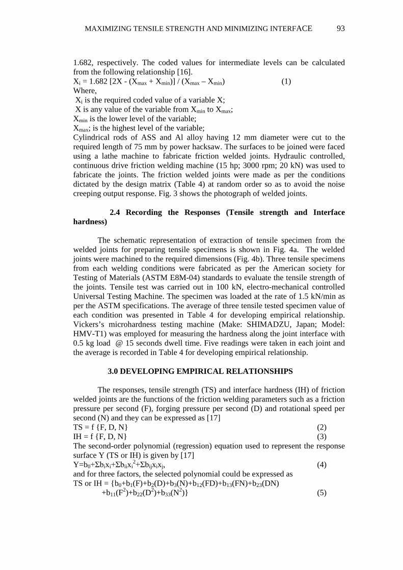
experimental errors. For a given set of independent variables, a characteristic surface is responded. When the mathematical form of Φ is not known, it can be approximated satisfactorily within the experimental region by a polynomial. Higher the degree of the polynomial the better is the correlation; but at the same time the costs of experimentation become higher. In this present investigation, RSM was applied for developing empirical relationships in the form of multiple regression equations for the quality characteristic of the friction welded dissimilar joints of ASS and Al. In applying the response surface methodology, the independent variable was viewed as a surface to which a mathematical model is fitted. 5.2 Contour Plots and Response Graphs Contour plots show a distinctive circular mound shape indicative of possible independence of factors with response. A contour plot is produced to visually display the region of optimal factor settings. For second order response surfaces, such a plot can be more complex than the simple series of parallel lines that can occur with first order models. Once the stationary point is found, it is usually necessary to characterize the response surface in the immediate vicinity of the point. Characterization means, identifying whether the stationary point found is a maximum response or minimum response or a saddle point. To classify this, the most straightforward way is to examine through a contour plot. Contour plots play a very important role in the study of the response surface. By generating contour plots using software for response surface analysis, the optimum is located with reasonable accuracy by characterizing the shape of the surface. If a contour patterning of circular shape occurs, it tends to suggest independence of factor effects while elliptical contours may indicate factor interactions [16]. Response surfaces have been developed for the models, considering two parameters in the middle level and plotting these in ‘X’ and ‘Y’ axes and response in ‘Z’ axis. The response surfaces clearly indicate the optimal response point. Figs. 6 and 7 show the contour plots and response graphs for the model developed for tensile strength of the joint and interface hardness of the joint (Eqns. 6 and 7). By analyzing the response surfaces and contour plots (Fig. 6), the maximum achievable tensile strength of the friction welded dissimilar joints of ASS and Al is found to be 181 MPa. By analyzing the response surface and contour plots (Fig. 7), the minimum achievable interface hardness of friction welded dissimilar joints of ASS and Al is found to be 124 Hv. The corresponding parameters that yielded the maximum tensile strength and minimum interface hardness are: friction pressure per second of 10 MPa/s, forging pressure per second of 10.25 MPa/s and rotational speed of 16.5 rev/s.
To validate and confirm the predictions of tensile strength and interface hardness by the RSM, three experiments were conducted by setting the optimized process parameter values. The experimental results, predicted values and percentage error between predicted and the experimental values are presented in Table 7. It is found from the results that the maximum percentage error is ±5%, which indicates the prediction capability of the developed optimization procedures.

96 G.VAİRAMANİ, T.Senthil KUMAR, S.MALARVİZHİ AND V.BALASUBRAMANİAN
Trakya Univ J Eng Sci, 13(2), 89-107, 2012
6.0 CONCLUSIONS
(i) Empirical relationships were developed to predict the tensile strength and interface hardness of friction welded dissimilar joints of AISI 304 austenitic stainless steel (ASS) and AA6082 aluminium alloy incorporating friction welding parameters.
(ii) The developed empirical relationships can be effectively used to predict the tensile strength and interface hardness of friction welded dissimilar joints of ASS and Al alloy at 95% confidence level.
(iii) A combination of friction welding parameters, namely, friction pressure per second of 10 MPa/s, forging pressure per second of 10.25 MPa/s and rotational speed of 16.5 rev/s yielded maximum tensile strength and minimum interface hardness for the dissimilar joints of ASS and Al alloy.
ACKNOWLEDGEMENTS
The authors also wish to record their sincere thanks to Dr.S.Rajakumar, Assistant Professor, Department of Manufacturing Engineering, Annamalai University, Annamalainagar for his help in statistical analysis. The authors are grateful to Dr.R.Paventhan, Associate Professor, Department of Mechanical Engineering, JJ College of Engineering, Tiruchirappalli for rendering help during fabrication of joints. REFERENCES
[1]. Ozdemir N. Investigation of mechanical properties of friction – welded joints between AISI 304 L and AISI 4340 steel as a function of rotational speed. Mater Lett 2005;59:2504–9.
[2]. Han-Ki Yoon, Yu-Sik Kong, Seon-Jin Kim, Akira Kohyama. Mechanical properties of friction welds of RAFs (JLF-1) to SUS 304 steels as measured by the acoustic emission technique. Fusion Eng Des 2006;81:945–50.
[3].Mumin Sahin, Erol Akata H, Turgut Gulmez. Characterization of mechanical properties in AISI 1040 parts welded by friction welding,Materials Characterization 58 (2007) 1033–1038.
[4]. Meshram S.D., T. Mohandas, G. Madhusudhan Reddy, Friction welding of dissimilar pure metals, Journal of Materials Processing Technology, (2007), 184, 330–337
[5]. Ozdemir N. F. Sarsılmaz, A. Hascalık, Effect of rotational speed on the interface properties of friction-welded AISI 304L to 4340 steel, Materials and Design 28 (2007), 301–307.
[6]. Mumin Sahin, Joining of stainless-steel and aluminium materials by friction welding; Int J Adv Manuf Technol (2009) 41:487–497.

MAXIMIZING TENSILE STRENGTH AND MINIMIZING INTERFACE 97
[7]. Sammaiah P, Tagore G R N, and Madhusudhan, G.R. Effect of parameters on mechanical properties of ferritic stainless steel(430) and 6063 Al aalloys by friction welding,Journal of Advanced Manufacturing Technology, Vol. 3 No. 1 January-June 2009
[8]. Mumin Sahin, M., Joining of aluminium and copper materials with friction welding”. Int J Adv Manuf Technol (2010) 49:527–534
[9]. Sammaiah P., Arjula Suresh, G. R. N. Tagore, Mechanical properties of friction welded 6063 aluminum alloy and austenitic stainless steel, J Mater Sci (2010) 45:5512–5521
[10]. Khalid Rafi H, Janaki Ram G D,. Phanikumar G, Prasad Rao K, Microstructure and tensile properties of friction welded aluminum alloy AA7075-T6, Materials and Design 31 (2010) 2375–2380.
[11]. Paventhan R, Lakshminarayanan PR, Balasubramanian V. Prediction and optimization of friction welding parameters for joining aluminium alloy and stainless steel. Transac. Of Nonferrous Metals Soc. Of China 2011; 21:342-349.
[12]. Sathiya, P. Aravindan, S. Noorul Haq, A. Mechanical and metallurgical properties of friction welded AISI 304 austenitic stainless steel [J]. Internaional Journal of Advanced Manufacturing and Technology, 2005, 26: 505–511. [13]. Ananthapadmanaban, D. A study of mechanical properties of friction welded mild steel to stainless steel joints [J]. Materials & Design, 2009, 30: 2642–2646.
[14]. Sathyanarayana, VV. Madhusudhan Reddy, G. Mohandas T. Dissimilar metal friction welding of austenitic–ferritic stainless steels [J]. Journal of Materials Processing and Technology, 2005, 60(2): 128–137.
[15]. Afes Hakan, Turker Mehmet, Kurt Adem. Effect of friction pressure on the properties of friction welded MA956 iron based super alloy [J]. Materials & Design, 2007, 28: 948–953.
[16]. Montgomery D.C. Design and Analysis of Experiments. 2001; 4th ed, John Wiley & Sons, New York.
[17]. Rajakumar S., Balasubramanian V. Correlation between weld nugget grain size, weld nugget hardness and tensile strength of friction stir welded commercial grade aluminium alloy joints, 2012 Materials and Design 34 , pp. 242-251.
[18]. Miller J.E, Freund, and Johnson R. Probability and Statistics for Engineers, 1996; Vol.5, Prentice Hall, New Delhi.

98 G.VAİRAMANİ, T.Senthil KUMAR, S.MALARVİZHİ AND V.BALASUBRAMANİAN
Trakya Univ J Eng Sci, 13(2), 89-107, 2012
Table 1 Chemical composition (wt %) of ASS and Al alloy
Elements C Mn Si P S Cr Ni Cu Fe Al ASS
(AISI304) 0.06 1.38 0.32 0.06 0.1 18.4 8.7 0.04 Bal 0.5
Al alloy (AA6082) -- 0.70 0.90 -- -- 0.25 -- -- 0.5 Bal
Table 2 Mechanical properties of ASS and Al alloy
Materials Yield strength (MPa)
Tensile strength (MPa)
Elongation in 50 mm
gauge length (%)
Reduction in cross
sectional area (%)
Micro hardness @ 0.5 kg (Hv)
ASS (AISI 304) 410 560 30 24 300
Al alloy (AA6082) 260 310 20 18 102
Table 3 Feasible working range of the friction welding parameters S.No. Parameter Notation Unit Levels
-1.682 -1.0 0 +1.0 +1.682 1 Friction
Pressure per second
F MPa/s 4 7.25 12 16.75 20
2 Forging pressure
per second D MPa/s 4 7.25 12 16.75 20
3 Rotational speed per second
N rev/s 12 15 18 21 24

MAXIMIZING TENSILE STRENGTH AND MINIMIZING INTERFACE 99
Table 4 Design Matrix and Experimental Results Expt. No.
F D N F (MPa/s)
D (MPa/s)
N (rev/s)
Tensile strength (TS) of
the joint (MPa)
Interface hardness (IH) of
the joint (Hv)
1 -1 -1 -1 7.25 7.25 15.25 126 163 2 +1 -1 -1 16.75 7.25 15.25 142 156 3 -1 +1 -1 7.25 16.75 15.25 145 138 4 +1 +1 -1 16.75 16.75 15.25 159 135 5 -1 -1 +1 7.25 7.25 21.75 123 160 6 +1 -1 +1 16.75 7.25 21.75 105 181 7 -1 +1 +1 7.25 16.75 21.75 139 152 8 +1 +1 +1 16.75 16.75 21.75 104 178 9 -1.682 0 0 4 12 18 128 162 10 +1.682 0 0 20 12 18 107 172 11 0 -1.682 0 12 4 18 120 163 12 0 +1.682 0 12 20 18 143 142 13 0 0 -1.682 12 12 15 145 136 14 0 0 +1.682 12 12 24 125 171 15 0 0 0 12 12 18 197 115 16 0 0 0 12 12 18 186 121 17 0 0 0 12 12 18 190 113 18 0 0 0 12 12 18 188 118 19 0 0 0 12 12 18 189 122 20 0 0 0 12 12 18 198 120

100 G.VAİRAMANİ, T.Senthil KUMAR, S.MALARVİZHİ AND V.BALASUBRAMANİAN
Trakya Univ J Eng Sci, 13(2), 89-107, 2012
Table 5 ANOVA Test Results for Tensile Strength Model
Source Sum of Squares
(SS)
Degrees of freedom
(df)
Mean Square (MS)
‘F’ Ratio
p-value Prob > F
Model 19497.93 9 2166.437 46.99242 < 0.0001 Significant F 249.0287 1 249.0287 5.401708 0.0425 D 588.9148 1 588.9148 12.77422 0.0051 N 1327.305 1 1327.305 28.79072 0.0003 FD 45.125 1 45.125 0.978811 0.3458 FN 861.125 1 861.125 18.67876 0.0015 DN 55.125 1 55.125 1.195722 0.2998 F2 8857.895 1 8857.895 192.1376 < 0.0001 D2 5674.015 1 5674.015 123.0757 < 0.0001 N2 4988.381 1 4988.381 108.2035 < 0.0001 Residual 461.0183 10 46.10183 Lack of Fit 337.685 5 67.537 2.737987 0.1466 Not
significant Std. Dev. 6.789 R-Squared 0.9769 Mean 147.95 Adj R-Squared 0.9561 C.V. % 4.5892 Pred R-Squared 0.8606 PRESS 2780.85 Adeq Precision 18.601

MAXIMIZING TENSILE STRENGTH AND MINIMIZING INTERFACE 101
Table 6 ANOVA Test Results for Interface Hardness Model
Source Sum of Squares
(SS)
Degrees of
freedom (df)
Mean Square (MS)
‘F’ Ratio
p-value Prob > F
Model 9637.004 9 1070.778 117.9321 < 0.0001 Significant F 212.0817 1 212.0817 23.35801 0.0007 D 624.0492 1 624.0492 68.7308 < 0.0001 N 1391.692 1 1391.692 153.2766 < 0.0001 FD 10.125 1 10.125 1.115135 0.3158 FN 406.125 1 406.125 44.72932 < 0.0001 DN 153.125 1 153.125 16.8647 0.0021 F2 4069.149 1 4069.149 448.1632 < 0.0001 D2 1965.013 1 1965.013 216.4203 < 0.0001 N2 2085.807 1 2085.807 229.7242 < 0.0001 Residual 90.79614 10 9.079614 Lack of Fit 27.96281 5 5.592562 0.445031 0.8025 Not
significant Std. Dev. 3.013 R-Squared 0.9906 Mean 145.9 Adj R-Squared 0.9825 C.V. % 2.065 Pred R-Squared 0.9689 PRESS 302.26 R-Squared 29.53 Table 7 Validation of optimization procedures
Optimized Process Parameters
Predicted Tensile Strength of
the joints (MPa)
Experimental Tensile Strength of
the joints (MPa)
Error (%)
F=10.00 MPa/s; D= 10.25 MPa/s; N= 16.50 rev/s
181 190 +4.9 174 -3.8 186 +2.7
Predicted Interface Hardness
of the joints (Hv)
Experimental Interface Hardness
of the joints (Hv)
124 120 -3.2 130 +4.8 119 -4.0

102 G.VAİRAMANİ, T.Senthil KUMAR, S.MALARVİZHİ AND V.BALASUBRAMANİAN
Trakya Univ J Eng Sci, 13(2), 89-107, 2012
(a) AISI 304 Austenitic Stainless Steel
(b) AA 6082 Aluminium alloy
Fig. 1 Optical micrographs of ASS and Al alloy

MAXIMIZING TENSILE STRENGTH AND MINIMIZING INTERFACE 103
(a) Friction pressure per second
(F) ˂ 4 MPa/sec (b) Friction pressure per second
(F) > 20 MPa/sec
(c) Forging pressure per second
(D) ˂ 4 MPa/sec (d) Forging pressure per second
(D) > 20 MPa/sec
(e) Rotational speed per second
(N) < 12 rev/sec (f) Rotational speed per second
(N) < 24 rev/sec
Fig. 2 Photographs of the joint fabricated outside the feasible working limits

104 G.VAİRAMANİ, T.Senthil KUMAR, S.MALARVİZHİ AND V.BALASUBRAMANİAN
Trakya Univ J Eng Sci, 13(2), 89-107, 2012
Fig. 3 Photograph of Friction welded ASS-Al Joints
( a) The schematic representation of extraction of tensile specimen
(b ) Tensile Specimen
(All dimensions are in mm) Fig.4 Dimensions of tensile specimen

MAXIMIZING TENSILE STRENGTH AND MINIMIZING INTERFACE 105
(a) Tensile strength model
(b) Interface Hardness model
Fig. 5 Correlation graphs
106 G.VAİRAMANİ, T.Senthil KUMAR, S.MALARVİZHİ AND V.BALASUBRAMANİAN
Trakya Univ J Eng Sci, 13(2), 89-107, 2012
(a) Contour plot between F and D (d)Response Graph between F and D
(b) Contour plot between F and N (e)Response Graph between F and N
(c) Contour plot between D and N (f)Contour plot between D and N
Fig. 6 Response Graphs and Contour Plots for Tensile Strength Model

MAXIMIZING TENSILE STRENGTH AND MINIMIZING INTERFACE 107
(a) Contour plot between F and D (d) Response Graph between F and D
(b) Contour plot between F and N (e) Response Graph between F and N
(c) Contour plot between D and N (f) Response Graph between D and N
Fig. 7 Response Graphs and Contour Plots for Interface Hardness Model

108 G.VAİRAMANİ, T.Senthil KUMAR, S.MALARVİZHİ AND V.BALASUBRAMANİAN
Trakya Univ J Eng Sci, 13(2), 89-107, 2012

The research conducted within this study has been supported by Trakya University Department of Scientific Research Projects with a project code number of TUBAP–2012–10.
http://fbe.trakya.edu.tr/tujs Trakya Univ J Sci, 13(2): 109-119, 2012 ISSN 2147–0308 DIC: 007DGET1321204130413
A WEB-CONTROL BASED STUDENT CLASSROOM ATTENDANCE TRACKING
SYSTEM APPLICATION: TUODS
Deniz Mertkan GEZGİN
Trakya Üniversitesi, Eğitim Fakültesi, Bilgisayar ve Öğretim Teknolojileri Eğitimi Bölümü, 22030 Edirne
e-mail: [email protected]
ABSTRACT
The focus matter of this study is to track the classroom attendance/absence of students
through digital techniques instead of paper-based methods. The purpose is to create and
implement an electronic, web-based student attendance tracking system in order to save from
paperwork expenses, to save lecture time by eliminating the need for roll calls via an online
processing fingerprint ID system and to report attendance/absence data over a student web
portal. The study required extensive research and investigation into the structure of biometric
fingerprint ID scanner devices and other elements that are required in order to integrate and
control these devices with computer software. Consequentially, a Web and Microsoft
Windows based computer software has been developed.
Keywords: Biometrics, Fingerprint, Attendance/Absence, Web
WEB KONTROL TEMELLİ BİR ÖĞRENCİ DEVAM/DEVAMSIZLIK TAKİP
SİSTEMİ UYGULAMASI: TUODS
ÖZET
Bu çalışmanın ana konusu, öğrenci devam/devamsızlık işleminin artık dijital ortamda
kontrol edilmesi ve hesaplanmasıdır. Amaç, maliyetten (kâğıt masrafı) tasarruf, öğrencilerin
sınıflara giriş yaparken parmak izi okuma cihazı ile çevrimiçi işlem sayesinde zamandan (ders
saatinden) tasarruf ve öğrenci web portalı ile devam/devamsızlık raporlama gibi işlemleri
yerine getirebilen bir Elektronik ve Web kontrolleri tabanlı bir devam/devamsızlık öğrenci
takip sistemi oluşturmaktır. Bu çalışma kapsamında biyometrik parmak izi okuyucusu
cihazların yapısı, yazılım ile bütünleşmiş çalışabilmesi için gerekli elemanları araştırılıp ve
Araştırma Makalesi / Research Article

110 Deniz Mertkan GEZGİN
Trakya Univ J Eng Sci, 13(2), 109-119, 2012
incelenmiştir. Bunun sonucu olarak bir Web ve Windows Tabanlı bir bilgisayar yazılım
programı geliştirilmiştir.
Anahtar Kelimeler: Biometri, Parmak izi, Devam/Devamsızlık, Web
INTRODUCTION
Especially when the fields of healthcare, security and education are considered, the use
of biometric devices in our country has been getting more and more popular recently.
(Sönmez et al., 2007). Among the various purposes of use for these devices are the follow-up
of employee arrival and departure times and monthly reporting of these. As for the public
sector, biometric devices combined with fingerprint identification tools are used in schools to
monitor the entries and exits of students from the building. Such systems are generally used at
a more hardware-oriented level and in combination with mechanisms such as turnstiles.
However, there’s still need for a system in which the hardware works along with a
sophisticated software component. Such a system could bring an electronic solution to
problems regarding the tracking of student classroom attendance in terms of security,
timeliness and paper waste. For this reason, a system that is comprised of a biometric
fingerprint ID device and a compliant software, which brings a solution to student classroom
attendance tracking problems, has been developed and implemented at the sample of Trakya
University Department of Computer Education and Instructional Technologies (CEIT)
students.
Today, tracking-automation systems that employ biometric devices are actively used
and new systems that closely follow the developments in the field of biometry keep emerging
rapidly. The most popular ones among these recent systems, which find use in the education
sector, are the student attendance tracking system from Perkotek Company (Perkotek,2010)
and the personal tracking system from Meyer (Meyer PDKS,2011).
In the development of the web-based student attendance tracking system application:
TUODS, the ASP.NET technology and the C# programming language have been used for the
web-side of the system, whereas C# programming language has been used for the Microsoft
Windows side.
The author shall provide information on biometrics and fingerprint ID systems in
Section 2, discuss the existing attendance tracking systems in schools or universities and point
out their disadvantages in Section 3, detail the hardware used in compliance with TUODS in
A WEB-CONTROL BASED STUDENT 111
Section 4, explain the attendance tracking software that has been developed and provide the
Unified Modeling Language (UML) diagram in section 5 and finally report the results and
provide recommendations in Section 6.
BIOMETRICS AND FINGERPRINT IDENTIFICATION
Biometrics is the science of verifying the identity of an individual by analysing
biological data, namely the physical attributes or the behavior of the individual ( Woodward
ve Ark., 2003). Among physical attributes are fingerprints, palm prints, hand geometry and
iris and face recognition. As for behavior patterns, autographs, voice and walking style can be
considered (Sönmez et al., 2007)
The biometric system scans an attribute or a behavior of an individual and compares it
to the pre-generated record stored within a database. The system scans attributes such as
fingerprints, hand shape or retina and hence needs to be extremely sensitive and accurate.
During the initial acquisition of the individual’s anatomical or physiological attributes,
accurate and repeated measurements must be made. All biometric systems need to possess the
five qualities stated below (Chellappa et al.,1995):
1. Universality: All individuals must carry the said biometric feature.
2. Uniqueness: The biometric characteristic should be different and unique in each individual
3. Constancy: The characteristic should remain constant through the passage of time.
4. Ease of Acquisition: The biometric feature should be easily acquired with practical tools.
5. Acceptability: Individuals should be consenting to the acquisition of the biometric feature
(Ergen and Çalışkan,2011)
As a first step, the records of authorized persons such as executives, employers or
teachers are entered into the biometric system. This process would take longer than the
normal acquisition of records. The reason for this longer duration is the need for acquiring
several samples of the same person’s attribute for the purpose of education. The number of
samples is usually two. As for the normal use, which is also referred to as the online mode,
the feature extraction process which is similar to data acquisition but carried out for a single
sample follows compression and decompression; after which the matching and decision
making stages are carried out. ( Kholmatov, 2003)

112 Deniz Mertkan GEZGİN
Trakya Univ J Eng Sci, 13(2), 109-119, 2012
Figure 1. The general operation structure of biometric systems (Şamlı and
Yüksel,2009)
The biometric identification systems that exist today are as follows:
• Hand (palm) geometry identification
• Facial recognition
• Blood Vein recognition
• Voice recognition
• Iris recognition
• Retinal recognition
• Fingerprint recognition
• Autograph recognition
Among the biometric methods that have been listed above in bullets, the methods that are
the easiest to implement, most cost-efficient, most common and most reliable in terms of
recognition are facial and fingerprint recognition methods (Daugman,1993). For the system
that is the subject of this study, the fingerprint identification biometric method has been
chosen. The fingerprint is a physically unique attribute in every human being (Chikkerur,
2005). The imitations of fingerprints can be prevented today with the use of aliveness-testing
fingerprint sensors ( Varlık and Çorumluoğlu ,2011). An automated fingerprint idenfitication
system (AFIS) that works with this principle usually relies on detecting feature anchor points

A WEB-CONTROL BASED STUDENT 113
in fingerprints and the comparison of the parameters of these with existing records (Sağıroğlu
and Özkaya, 2006).
Another interesting system recently developed in the field of biometrics is the palm-based
tracking system which scans blood vein patterns in the palm of the human hand. As of today,
individuals who seek services in the offices of the Turkish Social Security Institution found in
20 provinces are identified by palm prints rather than citizenship ID’s, driver’s licenses,
passports or certificate of marriage; therefore providing an effective solution against fraud and
similar forms of abuse.
EXISTING ATTENDANCE TRACKING PROCESSES AND THEIR
DISADVANTAGES
Currently, attendance tracking in schools is usually carried out with traditional pen and
paper methods, which has several disadvantages, such as:
• Paperwork expenses
• Loss of precious classroom time due to time taken in collecting signatures
• Students signing on behalf of their absent classmates
• Loss of attendance sheets causing the loss of all relevant attendance data
• Difficulty in accurately following up the attendance statuses of students for a
particular class, causing pressure on the lecturer.
An electronic system has been developed in order to overcome the said disadvantages.
The aim is to achieve the following:
• Entries into the attendance system made upon entering the classroom
• Singular key with a fingerprint ID system.
• Solution for the paperwork expenses.
• Providing attendance reports to students with web support
• Control provided to lecturers with updated administrative panel
• Secure processes, retrospective access

114 Deniz Mertkan GEZGİN
Trakya Univ J Eng Sci, 13(2), 109-119, 2012
THE HARDWARE USED WİTH THE STUDENT ATTENDANCE
TRACKING SYSTEM APPLİCATION AND THE SYSTEM FLOW STRUCTURE
The following hardware have been used for the creation of the TUODS System.
a- Fingerprint ID Scanner
A device that enables the acquisition of fingerprint data from students. Supports
TCP/IP, interface and audio feedback languages include Turkish, wall-mounted device can
store more than 3000 fingerprint ID records and hold more than 100000 log entries. Technical
specifications for the fingerprint ID scanner is as follows: Model ZKSoftware T4, Capacity:
3000 Fingerprints/50.000 Log Biometric Fingerprint Time Control (PDKS) and Optical Glass
Sensor, Ring alerts, TCP/IP, RS232/485 LCD Display ,Keypad.
b- Desktop or Laptop Computer
The software that runs on the Microsoft Windows side runs on a standard desktop or
laptop computer, which is connected to the fingerprint ID scanner and which the lecturer uses
to run the lecture modules on. Today, laptops are preferred more frequently due to mobility
and default wireless connectivity advantages. The specifications of the Desktop PC used for
the study is as follows: Intel Core i5 – 320 GHz processor, 6 GB’s of RAM, 560 GB HDD ,
17” LCD monitor, CPU case, keyboard, mouse and Windows 7 Ultimate-64 bit as operating
system.
c- Wireless Access Point
The connection between the computer and the fingerprint ID scanner is made via data
cables normally. However, it is also possible to connect the fingerprint ID scanner to a
wireless access point in order to establish connection between it and the computer. The
wireless connectivity standard to prefer is 802.11n. Technical specifications for the Wireless
Router used for the study is as follows: Asus RT-n13U , 1 x RJ45 for 10/100 BaseT Wan Port
, 4 x RJ45 for 10/100 BaseT Lan Ports , 1 x USB 2.0 Port and WPS.

A WEB-CONTROL BASED STUDENT 115
Şekil 2. The Operation of the Tuods System and the Hardware Infrastructure
SYSTEM SOFTWARE
This system software has been tested on the 4th year students of Trakya University
Faculty of Education Department of Computer Education and Instructional Technologies
during the Spring semester of the 2011-2012 academic year. The classroom attendance of 40
students have been tracked for one semester with this system. The system has been employed
through two modules namely the Windows-based instructor’s module and and web-based
student’s module.
a-Microsoft Windows Based Lecturer Module Software
The TUODS Windows based module works in compliance with the Fingerprint
scanner device. As shown in Figure 3, this module can connect to the fingerprint scanner
device in either wired or wireless modes. The lecturer may log on to the system with the
username and password that belongs to him and create virtual classrooms for departments that
he gives lectures in. When the time of the said class comes, he logs on at the respective virtual
classroom and proceeds to take into the classroom the students of the said class one by one,
acquiring their fingerprint ID’s in the process. He may choose to end the acquisition process
manually or set it to end after a predefined duration. He may generate reports regarding the
attendance data of the students and make changes on these. This software normally works on
a classroom computer or the lecturer’s mobile personal computer.
116 Deniz Mertkan GEZGİN
Trakya Univ J Eng Sci, 13(2), 109-119, 2012
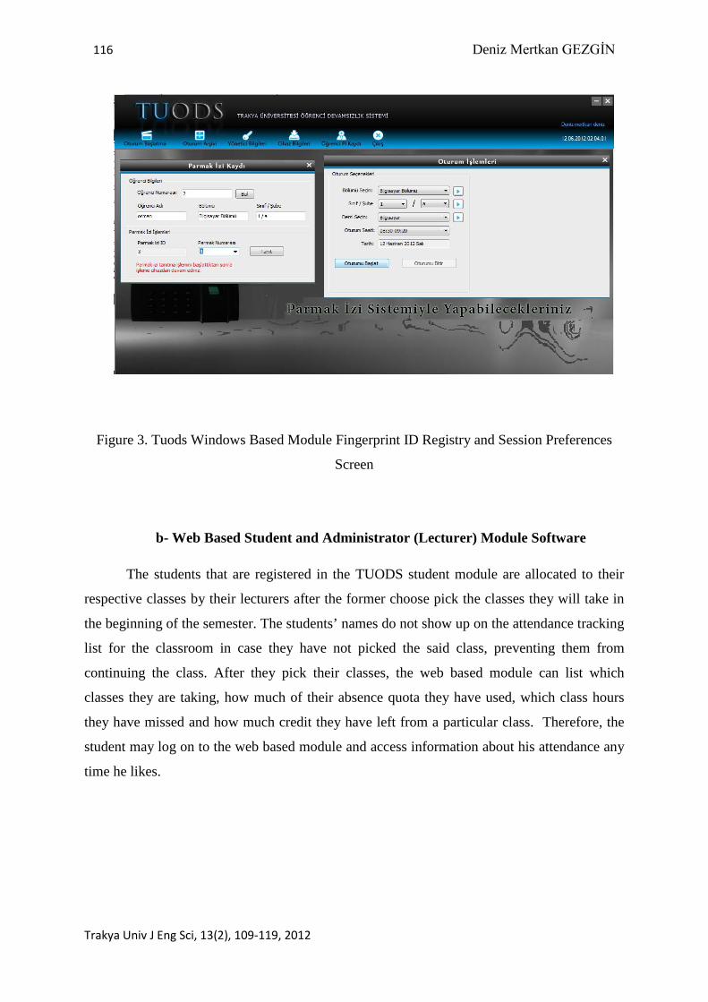
Figure 3. Tuods Windows Based Module Fingerprint ID Registry and Session Preferences
Screen
b- Web Based Student and Administrator (Lecturer) Module Software
The students that are registered in the TUODS student module are allocated to their
respective classes by their lecturers after the former choose pick the classes they will take in
the beginning of the semester. The students’ names do not show up on the attendance tracking
list for the classroom in case they have not picked the said class, preventing them from
continuing the class. After they pick their classes, the web based module can list which
classes they are taking, how much of their absence quota they have used, which class hours
they have missed and how much credit they have left from a particular class. Therefore, the
student may log on to the web based module and access information about his attendance any
time he likes.
A WEB-CONTROL BASED STUDENT 117
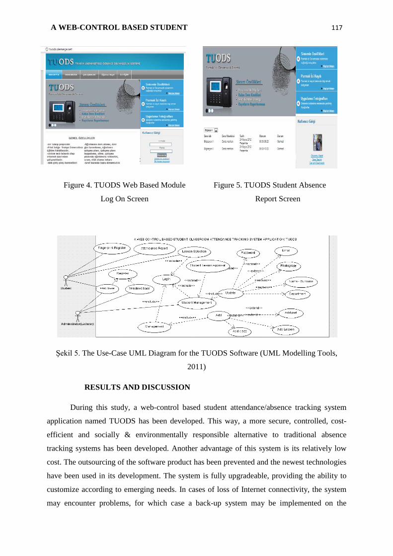
Figure 4. TUODS Web Based Module
Log On Screen
Figure 5. TUODS Student Absence
Report Screen
Şekil 5. The Use-Case UML Diagram for the TUODS Software (UML Modelling Tools,
2011)
RESULTS AND DISCUSSION
During this study, a web-control based student attendance/absence tracking system
application named TUODS has been developed. This way, a more secure, controlled, cost-
efficient and socially & environmentally responsible alternative to traditional absence
tracking systems has been developed. Another advantage of this system is its relatively low
cost. The outsourcing of the software product has been prevented and the newest technologies
have been used in its development. The system is fully upgradeable, providing the ability to
customize according to emerging needs. In cases of loss of Internet connectivity, the system
may encounter problems, for which case a back-up system may be implemented on the

118 Deniz Mertkan GEZGİN
Trakya Univ J Eng Sci, 13(2), 109-119, 2012
computer that holds the records and asynchronous syncing of the data on the computer may be
carried out once the connectivity has been restored. Keeping the accuracy of the fingerprint
ID scanner high may help the processes to take shorter time.
ACKNOWLEDGEMENTS
I would like to thank the Trakya University Department of Scientific Research
Projects, which has funded the research and my respected colleague Asst. Prof. Dr. Cem
Çuhadar, who has reviewed the article before printing and provided valuable advice.
REFERENCES
[1]. CHELLAPPA R., WILSON C. L., SIROHEY S., Human and machine recognition of
faces: A survey. Proceedings IEEE, 83(5):705-740, 1995.
[2].CHIKKERUR S. S., Online Fingerprint Verification System, Master Thesis, 2005 ,
StateUniversity of New York
[3].DAUGMAN J. G., High confidence visual recognition of persons by a test of statistical
independence, IEEE Trans. Pattern Analysis and MachineIntelligence, Vol. 15, No. 11, pp.
1148-1161, 1993.
[4].ERGEN B.,ÇALIŞKAN A., “Biyometrik Sistemler ve El Tabanlı Biyometrik Tanıma
Karakteristikleri”, 6th International Advanced Technologies Symposium (IATS’11), 455-
460,2011.
[5].KHOLMATOV A. A., Biometric Identity Verification Using On-Line & Off-Line
Signature Verification ,Springer.2003
[6].MEYER PDKS, http://www.meyer.com.tr/pdks.htm, 2011.
[7].PERKOTEK öğrenci Takip Sistemi, http://www.perkotek.com/12/220/detay/ogrenci-
takip-sistemi/, 2010.

A WEB-CONTROL BASED STUDENT 119
[8].SAĞIROĞLU Ş., ÖZKAYA N., Otomatik Parmak izi Tanıma Sistemlerinde Kullanılan
Önişlemler İçin Yeni Yaklaşımlar, Gazi Üniv.Müh. Mim. Fak. Der. Cilt 21, No 1, 11-
19,2006.
[9].SOSYAL GÜVENLİK KURUMU (SGK) , http://www.sgk.gov.tr/,2012
[10].SÖNMEZ E. B., ÖZBEK N. Ö., ÖZBEK Ö. , Avuç İzi ve Parmak İzine Dayalı Bir
Biyometrik Tanıma Sistemi, Akademik Bilişim’07 - IX. Akademik Bilişim Konferansı. 577-
582,2007, Kütahya.
[11].ŞAMLI R.,YÜKSEL M. E. , “Biyometrik Güvenlik Sistemleri”,Akademik Bilişim'09,
683-689,2009, Şanlıurfa
[12].UML BLOG ,http://univera-ng.blogspot.com/2009/11/uml-ve-modelleme-bolum-3-use-
case.html,2012
[13]. UML MODELLING TOOLS,http://argouml.tigris.org/,2011.
[14].VARLIK A., ÇORUMLUOĞLU Ö., Dijital Fotogrametri Teknikleri İle Kişi Tanıma ,
Harita Teknolojileri Elektronik Dergisi Cilt: 3, No: 2, 1-24, 2011.
[15].WOODWARD J. D., ORLANS N.M. , HIGGINS P. T. ,Biometrics, McGraw-Hill, 2003.

120 Deniz Mertkan GEZGİN
Trakya Univ J Eng Sci, 13(2), 109-119, 2012

http://fbe.trakya.edu.tr/tujs Trakya Univ J Sci, 13(2): 121-141, 2012 ISSN 2147–0308 DIC: 008ESET1321204130413
3D MODELLEMEDE KULLANILAN ARDIŞIK YANSITMALIYAPILANDIRILMIŞ
IŞIKYÖNTEMLERİ
1Eser SERT, 2Deniz TAŞKIN, 3Olcay ÖZCAN, 4Cem TAŞKIN, 5Kenan BAYSAL
1Trakya Üniversitesi, Edirne Teknik Bilimler Meslek Yüksekokulu, Elektronik Teknolojisi
Programı, Edirne
email:[email protected] 2Trakya Üniversitesi, Mühendislik Mimarlık Fakültesi, Bilgisayar Mühendisliği Bölümü,
Edirne
email:[email protected] 3Namık Kemal Üniversitesi, Hayrabolu Meslek Yüksekokulu, Bilgi Yönetimi Programı,
Tekirdağ
email: [email protected] 4 Trakya Üniversitesi, Tunca Meslek Yüksekokulu, Bilgisayar Teknolojisi Programı, Edirne
email:[email protected] 5Namık Kemal Üniversitesi, Hayrabolu Meslek Yüksekokulu, Bilgi Yönetimi Programı,
Tekirdağ
email: [email protected]
ÖZET
Yapılandırılmış ışık tekniği, nesnelerin 3D modellemesini gerçekleştirmede en
güvenilir temassız ölçüm yöntemlerinden birisidir. Yapılandırılmış ışık tekniğinde, kalibre
edilmiş kamera-projeksiyon çifti ve bilgisayar kullanılmaktadır. Projeksiyon, sahneye belirli
kodlama yöntemleri aracılığıyla kodlanmış desenleri yansıtmaktadır. Sonra, kamera
aracılığıyla bu desenlerin fotoğrafları alınmaktadır. Yansıtılan ve kameradan alınan desenler
arasındaki ilişki yorumlanarak 3D derinlik bilgisine ulaşılmaktadır. Yapılandırılmış ışık
sisteminde kullanılan kodlama yöntemi, elde edilecek 3D görüntünün kalitesini yakından
etkilemektedir. Bu çalışmada ardışık yansıtma temelli yöntemler incelenmiş ve bu yöntemler
çeşitli yönlerden karşılaştırılmıştır.
Araştırma Makalesi / Research Article

122 Eser SERT, Deniz TAŞKIN, Olcay ÖZCAN, Cem TAŞKIN, Kenan BAYSAL
Trakya Univ J Eng Sci, 13(2), 121-141, 2012
Anahtar Sözcükler: Yapılandırılmış ışık, 3D Modelleme, Üç Faz Kaydırma Algoritması,
Ardışık Yansıtma Yöntemleri
SEQUENTIAL PROJECTIVE STRUCTURED LIGHT METHODS USED FOR 3D
MODELING
ABSTRACT
Structured light technique is the most reliable contactless measurement method for the
realization of the 3D modeling of the objects. In the structured light technique, calibrated
camera-projection pairs and PC are used. The projection reflects the coded patterns, which
have been coded by specific methods, on to the scene. Then, the photos of these patterns are
taken by the camera. By making comment about projected and taken patterns from camera,
the 3D depth information can be reached. The coding method used for structural light system
will closely affect the quality of 3D image that will be obtained. In this study, sequential
projection based methods have been reviewed and this methods have been compared in
various ways.
Key Words: Structured Light, 3D Modeling, Three Phase Shifting, Sequential Projection
Methods
1. GİRİŞ
Klasik kameralarla alınan görüntüler2 boyutlu olduğundan derinlik bilgisi içermezler.
Bu durum gerçek dünyayı algılamakta sorunlar yaratabilmektedir. 3D teknolojisinin2 boyutlu
görüntülerden farklı olarak sunmuş olduğu derinlik bilgisi, nesnelerin sayısal sistemler
tarafından daha doğru yorumlanmalarına olanak sağlamaktadır. Bu avantajlardan dolayı 3D
görüntüleme teknolojileri savunma sanayi, tıp, eğitim ve sanayi alanlarında yaygınlıkla
kullanılmaktadır.
Son yıllarda 3D modelleme ve görüntüleme teknolojilerinde hızlı gelişmeler
yaşanmaktadır. Nesne ya da nesnelerin 3D modelini çıkarmak için kullanılan en etkili
çözümlerden birisi yapılandırılmış ışıkla modellemedir.
Bir yapılandırılmış ışık modeli,3D şekil ölçümü için Şekil 1’degörülmekte olan
kamera ve projeksiyon ikilisinden oluşan bir sistemi kullanmaktadır. Belirli yöntemler ile
kodlanan yapılandırılmış ışık desenlerini yansıtmak için projeksiyon makinesi kullanılır.

3D MODELLEMEDE KULLANILAN ARDIŞIK 123
Kamera ise sahnenin fotoğrafını bilgisayara aktarmaktadır. Sahne görüntüleri bilgisayar
tarafından işlenerek 3D bilgisine ulaşılmaktadır.
Şekil 1: Sahnede 3D nesne(Geng, 2011)
Bu görüntüler işlenirken, sahnede bulunan nesnenin yansıtılan yapılandırılmış ışıkta
meydana getirdiği bozulma miktarı dikkate alınmaktadır. Sahnede bulunan nesnenin derinlik
miktarına paralel olarak yapılandırılmış ışık deseninde bozulmalar meydana gelmektedir.
Benzer biçimde nesnenin derinliği sıfıra yaklaştığında, yapılandırılmış ışık desenindeki
bozulma da azalmaktadır.
Yapılandırılmış ışıkla üç boyutlu modelleme tekniğinde sahneye yansıtılan desenler
değişik kodlama türlerine sahip olabilmektedirler. Bu türlere örnek olarak ardışık yansıtma,
sürekli değişen, şerit indeksleme, ızgara indeksleme ve hibrit metotları verilebilir. Bu
çalışmada ardışık yansıtmalı (çoklu çekim) 3D yüzey görüntüleme teknikleri incelenmiştir.
2. 3D GÖRÜNTÜLEME TEKNİKLERİNİN SINIFLANDIRILMASI
Yapılandırılmış ışık ile 3D modellemede çeşitli yöntemler vardır. Bu yöntemler tekli
çekim ve çoklu çekim olarak iki ana gruba ayrılmaktadırlar. Ardışık yansıtma tekniklerinde
(çoklu çekim) birden fazla desen sahneye yansıtılıp fotoğrafları alınmaktadır. Tekil çekimde
ise sadece tek bir desen sahneye yansıtılıp fotoğrafı alınmaktadır. Yapılandırılmış ışık ile 3D
yüzey görüntüleme işleminde kullanılan teknik, elde edilecek 3D modelin performansını
yakından etkilemektedir. Bu çalışmada, Şekil 2’de görülmekte olan ardışık yansıtmalı 3D
yüzey görüntüleme tekniklerinin tamamı incelenmiştir.
Kamera Projektör

124 Eser SERT, Deniz TAŞKIN, Olcay ÖZCAN, Cem TAŞKIN, Kenan BAYSAL
Trakya Univ J Eng Sci, 13(2), 121-141, 2012
Ardışık Yansıtma Teknikleri (Çoklu Çekim)
İkili kod
Gray kod
Faz kaydırma
Hibrit: Gray kod + Faz kaydırma
Şekil 2:Yapılandırılmış ışık Temelli 3D Görüntüleme Tekniklerinin Sınıflandırılması
3.ARDIŞIK YANSITMA TEKNİKLERİ
Ardışık yansıtma teknikleri kendi arasında ikili kod, gray kod, faz kaydırma ve hibrit
tekniği olmak üzere dörde ayrılmaktadır
3.1 İkili Kod
Bu teknikte, 0 ve 1 olarak kodlanmış yalnızca iki aydınlatma düzeyi kullanılmaktadır.
0 ve 1,desende siyah ve beyaza karşılık gelmektedir. İkili desenin her pikseline karşılık gelen
kendi kodu mevcuttur; bu kod kelimeleri ise 0 ve 1’lerin sırasıyla belirlenmiştir. Bir kod
kelimesi yalnızca sıralama tamamlandığı zaman elde edilmektedir. Nesnenin yüzeyindeki her
bir nokta, diğer noktalardaki kodlamadan farklı benzersiz bir koda sahiptir. 1981’de ilk defa
Posdamer ve Altschuler tarafından desenin 2m şerit kodlayabildiği ortaya konmuştur. Şekil
3’te 5-bit’lik yansıtılan desen modelleri gösterilmektedir. Öncelikle bu desenler sırayla
sahneye yansıtılmaktadır. Böylece benzersiz şeritlerle 32 (25) adet farklı alan kodu
oluşturulur(Geng, 2011; Salvi vd. 2004).

3D MODELLEMEDE KULLANILAN ARDIŞIK 125
Şekil 3:3D Görüntüleme İçin İkili Kodlanmış Desen Yapısı
3.1.1 İkili Desenin Yansıtıldığı Resimde Piksel Yoğunluklarını Elde Etme
8 bit kapasiteli bir kameranın çıkış değer aralığı [0 255] arasındadır. Bu değer aralığı
ise Pon ve Poff olarak sınıflandırılabilmektedir. Piksel sınıflandırma metotları bu iki aralığın üst
ve alt sınırına göre belirlenmektedir.
İkili desen yansıtılan bir sahneden alınan görüntü Şekil 4’te verilmiştir(Xu ve Aliaga,
2007). Şekilde, ikili desenin beyaz (aydınlık) kısımlarına karşılık gelen bölgelerin yoğunluk
değeri [püst 255] arasında; siyah (karanlık) kısımlarına karşılık gelen bölgelerin yoğunluk
değeri [0 palt] arasındadır. Şekil üzerinde bu aralıklar kırmızı ve yeşil çizgiyle işaretlenmiştir.
Şekil 4:Eşikleme Yöntemiyle Pikselleri Sınıflandırma
Temel eşikleme yöntemi ile, pikselin p yoğunluğunun [0 palt] aralığına girdiğinde
Pkapalı olması, [püst 255] aralığına girdiğinde de Paçık olması sağlamaktadır. Bu şekilde
sahnedeki tüm pikseller sınıflandırılmaktadır. İkili şeridin bir periyodunu temsil eden
0 255
PÜst PAçık
255
PAlt PKapalı
Yüksek Değerli Bit Düşük Değerli Bit
Yansıtma Sırası

126 Eser SERT, Deniz TAŞKIN, Olcay ÖZCAN, Cem TAŞKIN, Kenan BAYSAL
Trakya Univ J Eng Sci, 13(2), 121-141, 2012
piksellerin sayısı Pn’dir. İkili dizi 1 numaralı denkleme bağlı olarak elde edilmektedir(Xu ve
Aliaga, 2007;Song vd., 2011).
Pkapalı(0)MOD [ Int (2x/ Pn) ] =0 (1) Bk(x,y) = Paçık(1) Değilse
Sahnede bulunan nesnelerin oluşturduğu gölgeler, nesne ya da zeminin geometrisinden
kaynaklanan sorunlar gibi faktörlerden dolayı piksel sınıflandırmada hatalar olabilmektedir.
Bu sorunları azaltmak için farklı sınıflandırma algoritmaları geliştirilmiştir.
3.1.2 İkili Kod temelli Kodlama ve Kod çözme
İkili desenin yansıtıldığı sahne görüntüsü kamera tarafından alınır. Alınan bu
desenlerin kesitlerinin aynı hizada paralel sıralanması sonucunda Şekil 5’teki görüntü elde
edilebilmektedir. Dört bitlik ikili sayı için 24-1 bağıntısına bağlı olarak 15 kenar oluşmaktadır.
Kod çözme sürecinin başlangıcında, kamera görüntülerinin pikselleri sınıflandırılarak
sayısallaştırılır. Ardından dört adet desenden alınan örnekleme noktalarına karşılık gelen ikili
değerler birleştirilerek kod kelimelerine ulaşılır. Örneğin sıra numarası 15 olan kesitin
örnekleme noktaları birleştirildiğinde ikilik tabanda 1111 sayısı elde edilmektedir. İkili
tabanda 1111’in onluk tabandaki kod karşılığı ise 15’tir. Bu şekilde ilgili kodun sıra
numarasına ve onluk tabandaki karşılıklarına ulaşılmaktadır. Elde edilen ikili kodlar derinlik
bilgisine ulaşmak için kullanılmaktadır.
Şekil 5: Zaman sırasına göre ikili desenlerin paralel dizilimi
Yüksek Değerli Bit (1111)2 =15
Düşük Değerli Bit
Yansıtma Sırası
1 2 3 4 5 6 7 8 9 10 11 12 13 14 15
1 2 3 4
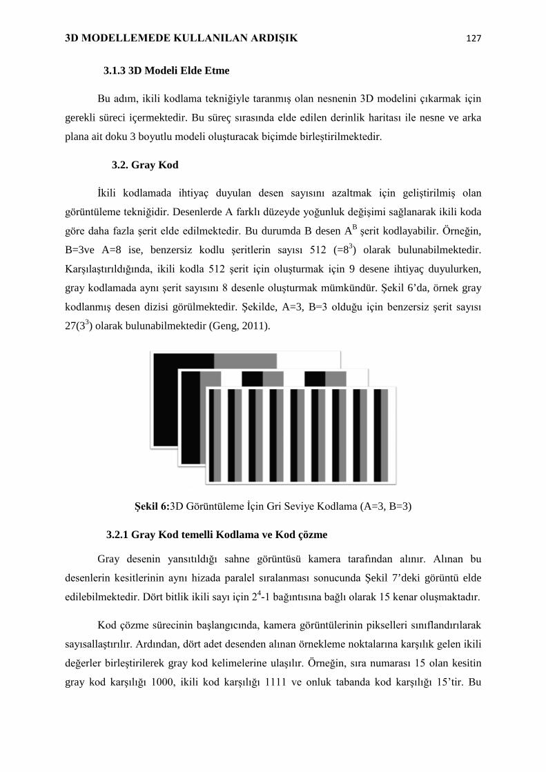
3D MODELLEMEDE KULLANILAN ARDIŞIK 127
3.1.3 3D Modeli Elde Etme
Bu adım, ikili kodlama tekniğiyle taranmış olan nesnenin 3D modelini çıkarmak için
gerekli süreci içermektedir. Bu süreç sırasında elde edilen derinlik haritası ile nesne ve arka
plana ait doku 3 boyutlu modeli oluşturacak biçimde birleştirilmektedir.
3.2. Gray Kod
İkili kodlamada ihtiyaç duyulan desen sayısını azaltmak için geliştirilmiş olan
görüntüleme tekniğidir. Desenlerde A farklı düzeyde yoğunluk değişimi sağlanarak ikili koda
göre daha fazla şerit elde edilmektedir. Bu durumda B desen AB şerit kodlayabilir. Örneğin,
B=3ve A=8 ise, benzersiz kodlu şeritlerin sayısı 512 (=83) olarak bulunabilmektedir.
Karşılaştırıldığında, ikili kodla 512 şerit için oluşturmak için 9 desene ihtiyaç duyulurken,
gray kodlamada aynı şerit sayısını 8 desenle oluşturmak mümkündür. Şekil 6’da, örnek gray
kodlanmış desen dizisi görülmektedir. Şekilde, A=3, B=3 olduğu için benzersiz şerit sayısı
27(33) olarak bulunabilmektedir (Geng, 2011).
Şekil 6:3D Görüntüleme İçin Gri Seviye Kodlama (A=3, B=3)
3.2.1 Gray Kod temelli Kodlama ve Kod çözme
Gray desenin yansıtıldığı sahne görüntüsü kamera tarafından alınır. Alınan bu
desenlerin kesitlerinin aynı hizada paralel sıralanması sonucunda Şekil 7’deki görüntü elde
edilebilmektedir. Dört bitlik ikili sayı için 24-1 bağıntısına bağlı olarak 15 kenar oluşmaktadır.
Kod çözme sürecinin başlangıcında, kamera görüntülerinin pikselleri sınıflandırılarak
sayısallaştırılır. Ardından, dört adet desenden alınan örnekleme noktalarına karşılık gelen ikili
değerler birleştirilerek gray kod kelimelerine ulaşılır. Örneğin, sıra numarası 15 olan kesitin
gray kod karşılığı 1000, ikili kod karşılığı 1111 ve onluk tabanda kod karşılığı 15’tir. Bu

128 Eser SERT, Deniz TAŞKIN, Olcay ÖZCAN, Cem TAŞKIN, Kenan BAYSAL
Trakya Univ J Eng Sci, 13(2), 121-141, 2012
şekilde ilgili kodun sıra numarasına ve onluk tabandaki karşılıklarına ulaşılmaktadır. Elde
edilen ikili kodlar derinlik bilgisine ulaşmak için kullanılmaktadır. Şekil 7’de,gray kodlu
desenlerin iç kenarları birbiriyle kesişmemektedir. Bu nedenle kodların değerlendirmesinde
hata yapma olasılığı düşmektedir.
Şekil 7:Zaman Sırasına Göre Gray Desenlerin Paralel Dizilimi
3.2.2. 3D Modeli Elde Etme
Bu adım, ikili kodlama tekniğiyle taranmış olan nesnenin 3D modelini çıkarmak için
gerekli süreci içermektedir. Bu süreç sırasında elde edilen derinlik haritası ile nesne ve arka
plana ait doku 3 boyutlu modeli oluşturacak biçimde birleştirilmektedir.
Şekil 8’de, yatay tarama ve eğri uygunlaştırma işlemine ait şekiller verilmiştir.
Modellenecek nesne üzerine gray desen yansıtılmış, i. hat taranmış ve her bir pikselin gri
değeri Şekil 8.b’de gösterilmiştir. Desenin filtrelenmesinden sonra gri seviyesinin sinyal
değişimi Şekil 8.c’de görülmektedir. Bu sinyalin üst ve alt limitlerine bağlı olarak ortalaması
bulunarak Şekil 8.c’de bu sonuç işaretlenmiştir. Bu işlemin sonunda kenar tespiti
gerçekleşmektedir(Wu vd., 2006).
1 2 3 4 5 6 7 8 9 10 11 12 13 14 15
1 2 3 4
Zaman Sırası
1000(Gray)=1111(İkili)=15(Onluk)
Sıra Numarası

3D MODELLEMEDE KULLANILAN ARDIŞIK 129
Şekil 8:Yatay tarama ve Eğri uygunlaştırma(Wu vd., 2006)
3.3 Faz Kaydırma
Faz kaydırma, 3D yüzey görüntüleme için iyi bilinen bir 3D görüntüleme metodudur.
Faz-kaydırma metodları yaygın avantajlarından dolayı ölçümlerde sıklıkla
kullanılmaktadır.Zhang, Sansoi Srinivasan vd. tarafından faz kaydırma tekniği konusunda
çalışmalar yapılmıştır.
3D modellemesi yapılacak nesne üzerine yansıtılacak saçak desenlerinin parlaklıkları
(Zhang, 2010):
I1(x,y)=I’(x,y) + I’’(x,y) cos[Ф(x,y)- 2π/3], (2)
I2(x,y) =I’(x,y) + I’’.(x,y)cos[Ф(x,y)], (3)
I3(x,y) =I’(x,y)+ I’’(x,y)cos[Ф(x,y) + 2π/3], (4)
olarak ifade edilebilmektedir. Burada I’(x,y) ortalama yoğunluk, I’’(x,y) yoğunluk
modülasyonudur.
a) i. Hattı Taranan Resim
b) Her Pikselin GrayDeğeri
Maksimum Değer
Minimum Değer c) Filrelenmiş Görüntünün Uygunlaştırma Eğrisi

130 Eser SERT, Deniz TAŞKIN, Olcay ÖZCAN, Cem TAŞKIN, Kenan BAYSAL
Trakya Univ J Eng Sci, 13(2), 121-141, 2012
Şekil 9:Sinüsoidal Sinyallere Karşılık Oluşan Saçak Resimleri
Denklem 2,3,4‘deki sinüzoidal sinyal denklemlerine karşılık oluşan saçak resimleri
Şekil 9’da görülmektedir.
3.3.1 3D Modeli Elde Etme
İlk olarak, I1 fazı nesne üzerine yansıtılırken kamera tarafından nesnenin görüntüsü
alınır. Aynı süreç I2 ve I3 fazı içinde gerçekleştirilmektedir.
I1, I2 ve I3 kullanılarak ortalama yoğunluk denklem 5’te bulunmuştur.
I′(x, y) = (𝐼1 + 𝐼2+𝐼3)/3 (5)
Yoğunluk modülasyonu denklem 6’da bulunmuştur.
I′′(x, y) = �𝟑(𝑰𝟏− 𝑰𝟑)𝟐+(𝟐𝑰𝟐−𝑰𝟏− 𝑰𝟑)𝟐
𝟑 (6)
Saçak Resimleri
Sinüsoidal Sinyaller I1 (α=-120°) I2 (α = 0) I3 (α=120°)

3D MODELLEMEDE KULLANILAN ARDIŞIK 131
Denklem 7’ye bağlı olarak faz matrisi elde edilmektedir (Karpinsky ve Zhang, 2010;
Zhang, 2010; Zhang ve Huang, 2006).
Faz :
Ф(𝐱,𝐲) = tan−1 (√𝟑 (𝐈𝟏− 𝐈𝟑)𝟐𝐈𝟐−𝐈𝟐−𝐈𝟑
) (7)
0-2π aralığındaki saçak desenlerinin faz değerleriyle wrapped resmi elde edilmektedir.
Wrapped sürecinden önce, üç faz resminin hesaplanan renk aralığına bağlı olarak bir maske
matrisikullanılır. Wrapped resim, resmin merkezinden başlayarak resim piksellerini tamamı
taranarak oluşturulmaktadır. Wrapped resim işlenerek unwrapped resim elde
edilir.Unwrapped derinlik bilgisi için yeterli değildir. Eğim açısı ve derinlik çarpanı
kullanılarak işlenmelidir. Bu adımın sonunda, z ekseni için derinlik bilgisi elde
edilmektedir(Zhang, 2010). Sistemin çalışmasını açıklayan akış şeması Şekil 10’da
görülmektedir.

132 Eser SERT, Deniz TAŞKIN, Olcay ÖZCAN, Cem TAŞKIN, Kenan BAYSAL
Trakya Univ J Eng Sci, 13(2), 121-141, 2012
Şekil 10:Üçlü Faz Kaydırma Algoritmasının Akış Şeması
3.4 Gray Kod+ Faz Kaydırma
Gray kodlar, piksel kodlamada zamanlama avantajı sağlamaktadır ancak desen
aralıkları sınırlıdır. Faz kaydırma metodunda ise periyodik olarak birkaç desen yansıtılıp
yüksek çözünürlüğe ulaşılabilmektedir. Her iki metodun avantajlarından yararlanabilmek için
birleştirilmeleriyle oluşturulmuş olan tekniktir. Böylece, yüksek çözünürlüğe sahip 3D
modellemeler yapılabilmektedir.
Gray ve faz kaydırma kod dizileri Şekil 11’de görüldüğü gibi 32 şeritli kodlama
sırasıyla kombine edilerek hibrit deseni elde edilmektedir.
Projektör Kamera
Faz
Wrapping
Wrapped Faz
Derinlik Haritası
3D Geometri
Unwrapping ve Derinlik
Haritasının Oluşturulması
3D Geometrinin
Oluşturulması
I1 I2 I3 I1 I2 I3

3D MODELLEMEDE KULLANILAN ARDIŞIK 133
Şekil 11:Faz Kaydırmayla Gray Kod Kombinasyonu (Gühring, 2000)
Bergmann, Sansoi, WioraGühring tarafından hibrit (gray kod + faz kaydırma)
tekniği üzerinde çalışmalar yapılmıştır. Şekil 12’de gray kod + faz kaydırma tekniğine ait
desen dizisi görülmektedir.
Şekil 12:Gray Kod+Faz Kaydırma
3.4.1 3D Modeli Elde Etme
Her bir piksel için denklem (8) ve denklem (9)’dan maksimum yoğunluk(Imax) ve
minimum yoğunluk (Imin) değerleri hesaplanmaktadır.
Imin(x,y) = I’(x,y)-I’’(x,y) (8)
Imak(x,y) = I’(x,y)+I’’(x,y) (9)
Gray Kod Dizisi
Faz Kaydırma Dizisi

134 Eser SERT, Deniz TAŞKIN, Olcay ÖZCAN, Cem TAŞKIN, Kenan BAYSAL
Trakya Univ J Eng Sci, 13(2), 121-141, 2012
Imin, Imakve𝐵𝑘 𝑛(𝑥,𝑦)kullanılarak normalizasyon işlemi denklem 10’abağlı olarak
gerçekleştirilmektedir (Song vd., 2011).
𝐵𝑘 𝑛(𝑥,𝑦) = 𝐵𝑘(𝑥,𝑦)−𝐼𝑚𝑖𝑛(𝑥,𝑦)
𝐼𝑚𝑎𝑘(𝑥,𝑦)−𝐼𝑚𝑖𝑛(𝑥,𝑦 (10)
Ardından, kod kelimesi denklem 11’e bağlı olarak hesaplanmaktadır.
CD(x,y) =∑ [2𝑁−𝑘−1𝐵𝑘𝑛𝑛𝑘=1 (𝑥, 𝑦)] (11)
Kod kelimesi kullanılarak faz değeri denklem 12’yebağlı olarak bulunmaktadır.
Ф(x, y) = Ф(x, y) + 𝐶𝐷𝑥2𝜋 (12)
(Song vd., 2011; Gühring, J., 2001)
Hibrit metodunun akış diyagramı Şekil 13’te verilmiştir. Başta, desenler sahneye
yansıtılıp fotoğrafları çekilmektedir. Ardından, bu resimler işlenerek kod kelimeleri üretilir.
Faz kaydırma algoritmasından elde edilen faz değeri ve kod kelimesi kullanılarak yeni faz
değeri elde edilir. Yeni faz değeri kullanılarak wrapped faz değeri bulunur. Sonra, unwrapped
faz işlemi yapılır. Son adımda ise, elde edilen uzaysal koordinatlara bağlı olarak 3D
modelleme gerçekleştirilir.
Şekil 13:Hibrit Metodunun Akış Diyagramı (Song vd., 2011)
Saçak Resimlerinin Elde edilmesi
İkili Resimlerin
Elde Edilmesi
İkili Resimler
Kod Kelimeleri
Wrapped Faz
Unwrapped Faz
3D Şekil

3D MODELLEMEDE KULLANILAN ARDIŞIK 135
4.DENEYSEL SONUÇLAR
İkili kodlama, gray kodlama ve hibrit tekniklerinin performanslarını karşılaştırmak
için yapılmışanalizlerin sonuçları Tablo 1’de sunulmuştur.
Tablo 1.Nesneler ve 3D Modelleme Sonuçları
Kodlama Yöntemi Nesne 3D Modeli
İkili Kodlama
Tekniği
(Giryesvd.,2008)
Gray Kodlama
Tekniği(Lanman ve
Taubin, 2009)
Hibrit Tekniği
(Reitemeiervd.,2004)
Tablo 1’de sunulanörneklerde; Giryes vd. tarafından obje üzerine ikili desen dizisi,
Lanman ve Taubin tarafından obje üzerine gray kodlama dizisi, Reitemeier vd. tarafından ise
obje üzerine hibrit tekniği kullanılarak desen dizisi yansıtılmıştır. Ardından, elde edilen
resimler işlenerek 3D modelleme işlemi gerçekleştirilmiştir. Elde edilen 3D modelleme
sonuçlarıTablo 1’in sonsütunundasunulmaktadır. Tablo 1’de de görüldüğü gibi en iyi 3D

136 Eser SERT, Deniz TAŞKIN, Olcay ÖZCAN, Cem TAŞKIN, Kenan BAYSAL
Trakya Univ J Eng Sci, 13(2), 121-141, 2012
modelleme çözünürlüğü hibrit tekniğiyle, en düşük 3D modelleme çözünürlüğü ise ikili
kodlama tekniğiyle elde edilmiştir.
Üçlü faz kaydırma algoritmasıyla yapmış olduğumuz test işlemlerinin sonuçlarıTablo
3’te sunulmuştur. Test sürecinin başlangıcında, Şekil 14.a’dagörülen modellenecek kişinin
üzerine birbiriyle 120° faz farkı olan üç adet faz desenisırayla yansıtılmış ve herbir desenin
görüntüsü kamera aracılığıyla alınmıştır. Kameradan alınan bu görüntüler Şekil 14.a’da
görülmektedir. Ardından, alınan bu görüntüler işlenerek Tablo 3’te görülen “Wrapped Faz
1”şekli elde edilmiştir. Wrapped resmi işlenerek unwrapped resmi elde edilmiştir. Sonra,
unwrapped faz kullanılarak derinlik analizi yapılmış ve Tablo 3’te görülen “Derinlik Haritası
1” elde edilmiştir. Son adımda, derinlik haritası kullanılarak 3D modelleme işlemi
gerçekleştirilmiştir. Analiz sonucunda elde edilen 3D modelleme sonuçları, Tablo 3’te “3D
Görünümler 1” kısmında sunulmuştur. Şekil 14.b’de görülen faz resimleri üzerindeaynı işlem
süreçleri yürütülerek Tablo 3’te görülen “Wrapped Faz 2”, “Derinlik Haritası 2” ve “3D
Görünümler 2” elde edilmiştir.
Şekil 14: Modellenecek Kişi Üzerine Faz Desenlerinin Yansıtılma Süreci
a) 3D Modellenecek Kişi ve Üç Faz Deseninin Kişi Üzerine Yansıtılması
b) 3D Modellenecek Kişi ve Üç Faz Deseninin Kişi Üzerine Yansıtılması

3D MODELLEMEDE KULLANILAN ARDIŞIK 137
Tablo 3. Üçlü Faz Kaydırma Tekniğiyle Elde Edilen 3D Modeller 3D Modellenecek
Kişi 1 Analiz Sonucu Elde Edilen Sonuçlar 1
Wrapped Faz 1 Derinlik Haritası 1
3D Görünümler 1
3D Görünüm 1 3D Görünüm 2 3D Görünüm 3
3D Modellenecek Kişi 2 Analiz Sonucu Elde Edilen Sonuçlar 2
Wrapped Faz 2 Derinlik Haritası 2
3D Görünümler 2
3D Görünüm 1 3D Görünüm 2 3D Görünüm 3
Sonuçlarını Tablo 3’te sunduğumuz bu deneysel çalışmada yalnızca üç faz deseni
kullanmamıza rağmen gray ve ikili kodlama sistemlerine göre daha yüksek, hibrit

138 Eser SERT, Deniz TAŞKIN, Olcay ÖZCAN, Cem TAŞKIN, Kenan BAYSAL
Trakya Univ J Eng Sci, 13(2), 121-141, 2012
kodlamayaise yakın çözünürlükte 3D modelleme gerçekleştirilmiştir.Şekil 14.a’da görülen 1.
kişi için 3D modeli elde etme süresi10,43 sn, 2.kişi için 3D modeli elde etme süresiise 12.86
sn’dir. Diğer algoritmalarda daha fazla desen işlendiği için 3D modeli elde etme süresi üçlü
faz kaydırma algoritmasına göre çok daha uzundur.
5.TARTIŞMA
İkili kodlama tekniği güvelidir ve zemin karakteristiklerine daha az duyarlıdır. Buna
karşın, yüksek çözünürlüğe ulaşmak için çok sayıda desene ihtiyaç duyulmaktadır. Bu durum
3D modelin oluşturulma zamanını uzatmaktadır.
Şekil 7’de görülebildiği gibi gray kodlu desenlerin iç kenarları birbiriyle
kesişmemektedir. Bu nedenle kodların değerlendirmesinde hata yapma olasılığı düşmektedir.
Bu açıdan ikili kodlanmış desenlere göre daha güvenlidirler. Gray kodlamada daha az desenle
ikili kodlamanın şerit sayısına ulaşılmaktadır. Örneğin, ikili kodla 512 şerit oluşturmak için 9
desene ihtiyaç duyulurken, gray kodlamada aynı şerit sayısını 8 desenle oluşturmak
mümkündür. Gray kodlamada, ikili kodlamada olduğu gibi yüksek çözünürlüğe ulaşmak için
çok sayıda desene ihtiyaç duyulmaktadır. Bu da 3D modelin oluşturulma zamanını
uzatmaktadır.
Üçlü faz kaydırma algoritmasında sahneye yalnızca üç adet desen yansıtılmaktadır. Bu
nedenle ardışık yansıtma yöntemleri içerisinde en az desene gereksinim duyulan tekniktir.
Buna karşın bu teknikle yüksek çözünürlüklü 3D görüntüler elde edilebilmektedir.Faz
kaydırma algoritmasının diğer avantajları, sahne zeminine daha az duyarlılık göstermeleri ve
ölçüm sonuçlarının ortamın ışık miktarının değişiminden az etkilemesidir. 3D modelleme
süresi diğer metotlara göre daha kısadır.
Hibrit yöntemi faz kaydırma algoritması ve gray kodlamanın özelliklerini
birleştirdiğinden yüksek çözünürlükte 3D görüntüler elde edilebilmektedir. Buna karşın,
modellenecek nesne üzerine çok sayıda desen yansıtmaya gereksinim duymaktadırlar.
Desenler yansıtılırken nesnenin uzun süre hareketsiz olması gerektiğinden hareketli
görüntülerde uygulamak elverişli değildir. Ayrıca çok sayıda desenin bilgisayar tarafından
işlenmesine ihtiyaç duyulduğundan 3D görüntüyü elde etme süreci uzundur(Geng, 2011).

3D MODELLEMEDE KULLANILAN ARDIŞIK 139
6. SONUÇ
Bu çalışmada, ardışık yansıtmalı yapılandırılmış ışık teknikleri incelenmiş; her bir
tekniğin kullandığı desen yapısı ve kod çözme sistematiği sunulmuştur. Seçilen teknikler
üzerinde yapılan testlere bağlı olarak avantaj ve dezavantajları ortaya konmuştur.
Üçlü faz kaydırma algoritmasıyla az desenle yüksek performans elde edilmektedir.
Hibrit, ikili ve gray kodlama tekniklerinde çok sayıda desen kullanımıyla yüksek kalitede 3D
görüntüler elde edilmektedir. Ancak, çok sayıda desen kullanımı dezavantajlar
doğurmaktadır. Bu nedenle üçlü faz kaydırma algoritmasının diğer tekniklere göre daha
avantajlı olduğu görülmüştür.
KAYNAKÇA
[1].GENG, J.Structured-Light 3D Surface Imaging A Tutorial.Advances In Optics And
Photonics. 3: 128-160, 2011.
[2].GIRYES, R., BRONSTEIN, A. M., MOSHE, Y., BRONSTEIN, M. M. Embedded System
for 3D Shape Reconstruction.Proc. of the 3rd European DSP Education and Research
Symposium (EDERS 2008).265-272, 2008, Telaviv.
[3].GÜHRİNG, J.Dense 3-D surface acquisition by structured light using off-the-shelf
components.Photonics West, Videometrics VII. 4309, 2011, USA.
[4].GÜHRING, J., BRENNER, C., BÖHM, J., FRITSCH, D. Data Processing and Calibration
ofa Cross-Pattern Stripe Projector.International Archives of Photogrammetry and Remote
Sensing.XXXIII, 2000, Amsterdam.
[5].HE, Y., CAO, Y. A. Composite-Structured-Light 3D Measurement Method Based On
Fringe Parameter Calibration.Opticsand Lasers in Engineering. 49:773-779, 2011.
[6].HUANG, P. S., ZHANG, S. Fast Three-Step Phase-Shifting Algorithm. Applied
Optics.45:5086-5091, 2006.
[7].KARPINSKY, N., ZHANG, S. High-Resolution, Real-Time 3D Imaging With Fringe
Analysis.Journal of Real-Time Image Processing.7:55-66, 2012.

140 Eser SERT, Deniz TAŞKIN, Olcay ÖZCAN, Cem TAŞKIN, Kenan BAYSAL
Trakya Univ J Eng Sci, 13(2), 121-141, 2012
[8].LANMAN, D., TAUBIN, G. Build Your Own 3D Scanner: 3D Photography for Beginner,
SIGGRAPH 2009 Course Notes, USA, 2009.
[9].REITEMEIER, B., NOTHI, G., HEINZE, M., SCHÖNE, C., SCHMIDT, A., FICHTNER,
D.The Journal of Prosthetic Dentistry.Optical Modeling ofExtraoral Defects.91:80-84, 2004.
[10].ROCCHINI, C., CIGNONI, P., MONTANI, C. A Low Cost 3D Scanner Based On
Structured Light.Computer Graphics Forum. 20:299-308, 2002.
[11].SALVI, J., FERNANDEZ, S., PRIBANIC, T., LLADO, X.A State Of The Art in
Structured Light Patterns for Surface Profilometry.Pattern Recognition. 43:2666-2680, 2010.
[12].SEO, B. K., LEE, M. H., PARK, H., PARK, J. I., KIM, Y. S. Direct-Projected AR Based
Interactive User Interface for Medical Surgery.17th International Conference on Artificial
Reality and Telexistence.IEEE Computer Society,S. 105-112, 2007, Denmark.
[13].SALVI, J., PAGES, J., BATTLE, J.Pattern Codification Strategies in Structured Light
Systems.Pattern Recognition. 37:827-849, 2004.
[14].SONG vd.,Patent Application Publication, Pub. No.: US 2011/0080471 A1
(YayınlanmaTarihi: 07/04/2011).
[15].XU, Y., ALIAGA, D.G. Robust Pixel Classification for 3D Modeling with Structured
Light.Appeared in Proceedings of 33rd Graphics Interface Conference (GI). S. 233-240,2007,
Canada.
[16].WU, H.B., CHEN, Y., WU, M.Y., GUAN, C.R., YU, X.Y. 3D Measurement Technology
by Structured Light Using Stripe-Edge-Based Gray Code.Journal of Physics: Conference
Series 48.S. 537-541, 2006, China.
[17].ZHANG, S.High-Resolution, High-Speed 3-D Dynamically Deformable Shape
Measurement Using Digital Fringe Projection Techniques, S. 29-50, 2010. [Editor: Milind Kr
Sharma, Advances in Measurement Systems, ISBN: 978-953-307-061-2in Book: Advances in
Measurement Systems].
[18].ZHANG, S.Recent Progresses On Real-Time 3d Shape Measurement Using Digital
Fringe Projection Techniques.Optics and Lasers in Engineering. 48:149–158, 2010.

3D MODELLEMEDE KULLANILAN ARDIŞIK 141
[19].ZHANG, S., HUANG, P.S.Novel Method for Structured Light System
Calibration.Optical Engineering,Instrumentation, Measurement, and Metrology.45:1-8,2006.
[20].ZHANG, S., YAU, S.T. High-Resolution, Real-Time 3D Absolute Coordinate
Measurement Based On A Phase-Shifting Method.Optics Express. 14:2644–2649, 2006.
[21].ZOLLMANN, S., LANGLOTZ, T., BIMBER O. Passive-Active Geometric Calibration
for View-Dependent Projections onto Arbitrary Surfaces.Journal of Virtual Reality and
Broadcasting. 4: 1-10,2007.

142 Eser SERT, Deniz TAŞKIN, Olcay ÖZCAN, Cem TAŞKIN, Kenan BAYSAL
Trakya Univ J Eng Sci, 13(2), 121-141, 2012

http://fbe.trakya.edu.tr/tujs Trakya Univ J Sci, 13(2): 143-156, 2012 ISSN 2147–0308 DIC: 009ESET1321204130413
VHDL KULLANILARAK FPGA İLE YÜKSEK KAPASİTELİ TOPLAYICIÜNİTE TASARIMI
Deniz TAŞKIN1, Kenan BAYSAL2, Eser SERT3, Cem TAŞKIN4, Murat Olcay
ÖZCAN5
1Trakya Üniversitesi, Mühendislik Mimarlık Fakültesi, Bilgisayar Mühendisliği
Bölümü, Edirne
email: [email protected] 2Namık Kemal Üniversitesi, Hayrabolu Meslek Yüksekokulu, Bilgi Yönetimi
Programı, Tekirdağ
email:[email protected] 3Trakya Üniversitesi, Edirne Teknik Bilimler Meslek Yüksekokulu, Elektronik
Teknolojisi Programı, Edirne
email: [email protected] 4Trakya Üniversitesi, Tunca Meslek Yüksekokulu, Bilgisayar Teknolojisi Programı,
Edirne
email:[email protected] 5Namık Kemal Üniversitesi, Hayrabolu Meslek Yüksekokulu, Bilgi Yönetimi
Programı, Tekirdağ
email:[email protected]
ÖZET
Alan Programlanabilir Kapı Dizileri (FPGA), esnek tasarım kapasitesi ve
araştırma geliştirme aşamalarındaki uygun maliyetleri sebebiyle sayısal sistemlerde
en çok tercih edilen donanım platformlardandır. FPGA sistemlerinin tercih
edilmesindeki en önemli neden, deneme ve yanılma metoduyla karmaşık devreler
Araştırma Makalesi / Research Article

144 Deniz TAŞKIN, Kenan BAYSAL, Eser SERT, Cem TAŞKIN, Murat Olcay
ÖZCAN
Trakya Univ J Eng Sci, 13(2), 143-156, 2012
oluşturmak yerine Yüksek Hızlı Donanım Tasarlama Dili (VHDL) ile binlerce kez
programlanabilmeleridir.
Şifreleme biliminin bilgisayar teknolojisi ile birleşmesi ile birlikte artan güvenlik
sunan algoritmaların yüksek kapasiteli veriler ile çalışmaya başladığı görülmektedir.
Yüksek kapasiteli verilerin işlenmesindeki en büyük sorun veri işleme süresi ve
gelişmiş donanım yapılarına ihtiyaç duymalarıdır. Bu çalışmanın amacı yüksek
kapasiteli verileri işleyebilecek bir donanım tasarımı gerçekleştirerek veri işleme
süresini kısaltılmaktır.
Anahtar Kelimeler:FPGA, VHDL, kriptoloji, bilgisayar aritmetiği, yüksek
kapasiteli aritmetik toplayıcı

VHDL KULLANILARAK FPGA 145
DESIGNING HIGH CAPACITY ARTIHMETIC UNIT WITH FPGA
USING BY VHDL
ABSTRACT
Field Programmable Gate Arrays (FPGA) are most preferred hardware platforms
at digital systems, because of flexible design capacity and cheap cost at the research
and development level. The reason of preference FPGA systems, instead of building
complex circuits at the try and error method are could be program thousands of times
using by Very High Speed Hardware Design Language (VHDL)
With the merging of computer technology and cryptography science, algorithms,
that provide increased security, are started to working with high capacity data. The
biggest issue of processing high capacity data is processing time and needs to
advanced hardware structure. The aim of this study is to shorten the duration of data
processing by practicing to design of hardware that able to process high capacity
data.
Keywords: FPGA, VHDL, cryptology, computer arithmetic, high capacity
arithmetic adder

146 Deniz TAŞKIN, Kenan BAYSAL, Eser SERT, Cem TAŞKIN, Murat Olcay
ÖZCAN
Trakya Univ J Eng Sci, 13(2), 143-156, 2012
GİRİŞ
Bilgisayarda gerçekleştirilen veri işleme, kod çalıştırma ve hesaplama
işlemlerinin çoğu toplama işlemine dayanır. Bu işlemler ikili sistem tabanlı olarak
gerçekleştirilmektedir. Bilgisayarın veri işleme kapasitesine bağlı olarak toplama
işlemi yapılacak olan veri, aritmetik üniteye alınır. Veri boyutu aritmetik ünitenin tek
seferde işleyebileceğinden fazla ise, veri, paketler halinde bölünerek her saat
vuruşunda aritmetik ünitenin işleyebileceği kadar olan kısmı iletilir ve işlenir. Bu
durumda toplama işleminden artan elde kısmı taşma bayrağı ile bir sonraki saat
vuruşunda işlenecek olan pakete aktarılır (Hwang, 2004).
Şekil 1:Aritmetik İşlem Birimi
Aritmetik işlem biriminde aynı anda toplanacak bit sayısı arttığında işlem
sürecide uzayacaktır. Ancak, toplayıcının aynı anda işlemiş olduğu bit sayısı
arttırılarak işlem süreci kısaltılabilmektedir. Bu çalışmada FPGA platformu
kullanılarak yüksek hızlı toplayıcı devre tasarımı gerçekleştirilmiştir (Harris ve
Harris, 2007).
ARİTMETİK İŞLEM BİRİMLERİNDE TOPLAMA İŞLEMİ
Onluk sistemde basit bir toplama işlemi örneği Şekil 2’de görülmektedir.

VHDL KULLANILARAK FPGA 147
Şekil 2: Tek Basamaklı Toplama İşlemi
Bir basamaklı bir aritmetik ünite varsa bir saat vuruşu içinde bir basamaklı bir
toplama işlemi gerçekleştirir ve aynı saat vuruşu içinde elde basamağına artanı
gönderir. Şekil 2’de bu durum görülmektedir.
Bir basamaklı aritmetik toplayıcı kullanılarak iki basamaklı iki rakamın toplama
işlemi Şekil 3’te verilmiştir.
Şekil 3: İki Saat Vuruşu Süresinde Hatalı İki Basamaklı Toplama İşlemi
18 ile 12 sayılarının toplama işleminde, bir saat vuruşu içerisinde ilk basamakta
yapılan işlemin sonucunda oluşan elde değeri diğer basamağın sonucunu
etkilemektedir. Ancak bir saat vuruşu içerisinde elde aktarımı mümkün
olamamaktadır. Şekil 4’te görüldüğü gibi, toplama işleminin yapılabilmesi ve birinci
basamakta oluşan elde değerinin bir sonraki basamağın toplamına aktarılabilmesi
için iki saat vuruşundan fazla süre gerekmektedir (Paar ve Jan, 2010).
+
8
2
0 2 sonuç sonuç
2 saat vuruşu
1
1
+
8
2
0 1 sonuç elde
1 saat vuruşu

148 Deniz TAŞKIN, Kenan BAYSAL, Eser SERT, Cem TAŞKIN, Murat Olcay
ÖZCAN
Trakya Univ J Eng Sci, 13(2), 143-156, 2012
Şekil 4: İki Basamaklı Toplama İşlemi
Tablo 1’de, günümüzde kullanılan 32 bitlik ve 64 bitlik işlemcilerin 1 saat
vuruşunda işleyebildikleri veri boyutları ve 1024 bitlik bir veriyi işleme süreleri
görülmektedir.
Tablo 1. 32 bit 64 bit işlemci ile işlenebilecek veri boyutlarının karşılaştırılması
32 bit 64 bit
32 bit işlemci
32 bit işletim sistemi
32 bit derleyici
64 bit işlemci
64 bit işletim sistemi
64 bit derleyici
1 saat vuruşunda
4 byte’lık veri
işlenebilir
1 saat vuruşunda
8 byte’lık veri
işlenebilir.
1024 bitlik bir
toplama işlemi için
32 saat vuruşundan
daha fazla
1024 bitlik bir toplama
işlemi için
16 saat vuruşundan
daha fazla
Günümüzde kullanılan şifreleme algoritmalarının anahtar uzunluklarının 2048
bit boyutlarında olduğunu düşünülürse, her anahtar için şifreleme algoritmasının
işlenme süresi oldukça uzun süreler almaktadır (Buluş, 2006).
+
8
2
0 3 sonuç sonuç
2 saat vuruşundan fazla
1
1
1 elde

VHDL KULLANILARAK FPGA 149
TOPLAYICI TASARIMI
Yüksek kapasiteli verilerin işlenmesinde karşılaşılan uzun süre gereksinimi
sorununa çözüm olarak FPGA ile doğrudan anahtar boyutuna uygun kapasitede bir
aritmetik ünite tasarlanabilir. Standart bir tasarım sürecinde milyonlarca transistor
kullanılarak gerçekleştirilen bu işlem süreci,FPGA üzerine sadece birkaç VHDL
kodunun yüklenmesi ile gerçekleştirilebilir (Aydın,2005).
Şekil 5:1024 bit toplayıcı blok şema
1024 bitlik devrede bulunan bir bitlik bir toplayıcı devresinin uygun şekilde
genişletilmesi yoluyla toplama kapasitesi arttırılabilmektedir(Chen ve Ark., 2006).
Tek bitlik toplayıcının VHDL kodları tablo 2’de ve RTL görüntüsü Şekil 6’da
verilmiştir. Bu devrenin ModelSIM benzetim sonuçları ise Şekil 7’de verilmiştir.

150 Deniz TAŞKIN, Kenan BAYSAL, Eser SERT, Cem TAŞKIN, Murat Olcay
ÖZCAN
Trakya Univ J Eng Sci, 13(2), 143-156, 2012
Tablo 2.Tek bit toplayıcı VHDL kodları
libraryieee; useieee.std_logic_1164.all; useieee.std_logic_unsigned.all; useieee.std_logic_arith.all;
entityobfaddis port( A_BIT : in std_logic; B_BIT : in std_logic; C_BIT : in std_logic; COUT : outstd_logic; SUM_BIT : outstd_logic);
Endobfadd;
Architecturestructofobfaddis begin process(A_BIT, B_BIT, C_BIT) begin SUM_BIT <= (A_BIT xor B_BIT) xor C_BIT; COUT <= (A_BIT and B_BIT) or (A_BIT and C_BIT) or (B_BIT and
C_BIT); Endprocess;
Endstruct;
Şekil 6:Tek bit toplayıcı RTL görünüşü
Şekil 7: Tek bit toplayıcı ModelSIM benzetim sonuçları

VHDL KULLANILARAK FPGA 151
n’bitlik bir toplayıcı devresi oluşturabilmek için tek bit toplayıcı devresinden n
sayıda kullanılmalıdır.Bu çoğaltma işlemi, Tablo 3’te VHDL kodları verilen yapıda
“entity” kısmında tanımlanan “generate” bölmesinde “SZ” genişletilebilir değişken
boyutu olarak tanımlanmıştır (Ashenden, 1990).
Tablo 3. 64 bit toplayıcı VHDL kodları

152 Deniz TAŞKIN, Kenan BAYSAL, Eser SERT, Cem TAŞKIN, Murat Olcay
ÖZCAN
Trakya Univ J Eng Sci, 13(2), 143-156, 2012
Tablo 3’te VHDL kodları verilen 64 bitlik toplayıcı için veriler dışarıdan
verilmek yerine kod içerisinde “generic” bölümünde ROM olarak tanımlanmıştır. 64
bitlik toplayıcıda 64 bit A veri girişi, 64 bit B veri girişi, 64 bit SUM çıkışı, elde ve
kontrol bitleri ile 200 bit giriş çıkış pin sayısını geçmemektedir. Ancak 1024 ve 2048
bit gibi yüksek kapasiteli tasarımlarda giriş ve çıkışlarının toplamı FPGA’nın fiziksel
sınırlarını aşmaktadır. Bu yüzden işlenecek verinin içeride bir RAM veya ROM
bellek bölgesinde tutulması zorunludur.
DENEYSEL SONUÇLAR
Yapılan deneyler benzetim seviyesindedir. Deneysel amaçla kullanılan
donanımlar toplam veri giriş ve çıkışları işlenen veriyi doğrudan görüntülemede
yetersiz kalmaktadır (Munoz ve Ark., 2010). Bu sebeple gerçekleştirilen deneyde
veriler FPGA içerisinde tanıtılan sabit hafıza içerisinden kullanılmıştır. Çıkış verisi
de sabit hafıza içerisine kaydedilmiştir.
Benzetim sonuçlarının kolay görüntülenebilmesi için A girişinin 64 bitlik veri
değeri için en yüksek değerlikli biti “1” olarak seçilmiştir. Bu değer ise 263 =
(9223372036854775808)10 sayı değerine karşılık gelmektedir. B girişinin 64
bitlik veri değeri için 62. biti “1” olarak seçilmiştir. Bu
değer262 = (4611686018427387904)10 sayı değerine karşılık gelmektedir. Şekil
8 ve Şekil 9’daModelSIM benzetim sonuçları görülmektedir.
Şekil 8’de görüldüğü gibi sadece bir saat vuruşunda 64 bitlik iki verinin toplama
işlemi gerçekleştirilmiştir.
Tablo 3’te verilen kodların aynısı kullanılarak 1024 bitlik bir toplayıcı devresi
gerçekleştirilebilir. Sadece “generic” kısmında tanımlanan “SZ” boyutunun 1023
olarak değiştirilmesi ile A, B veri alanlarının 1024 bit boyutuna ayarlanarak1024 bit
boyutunda veri ile doldurulmasını gerektirmektedir.

VHDL KULLANILARAK FPGA 153
Şekil 8:64 bit toplayıcı ModelSIM benzetim sonuçları
ModelSIM benzetim sonuçları aşağıdaki şekilde verilmiştir.
Şekil 9:1024 bit toplayıcının ModelSIM benzetim sonuçları

154 Deniz TAŞKIN, Kenan BAYSAL, Eser SERT, Cem TAŞKIN, Murat Olcay
ÖZCAN
Trakya Univ J Eng Sci, 13(2), 143-156, 2012
Benzetim sonuçlarının kolay görülebilmesi için önceki örnekte olduğu gibi A
girişinin en yüksek değerlikli biti “1” olarak seçilmiştir. 21023 ≅ (89 𝑥 10306)10B
ifadesinde de en yüksek değerlikli bitin bir solundaki bit “1” olarak seçilmiştir.
21022 ≅ (45 𝑥 10306)10eşitliğibulunabilmektedir.
TARTIŞMA VE SONUÇ
Yüksek güvenlikli şifreleme algoritmalarında kullanılan yüksek basamaklı
anahtar boyutlarından dolayı karşılaşılan, donanım seviyesindeki yetersizliklere
FPGA ile tasarlanan işleme özgü yüksek basamaklı aritmetik üniteler ile çözüm
bulunmaktadır (Kawakami ve Ark.. 2008; M. Bečvář ve Štukjunger, 2005). Yazılım
destekli çözümlerde karşılaşılan sorunları aşabilme konusunda FPGA tasarımcıya
esnek bir platform sunmaktadır. Hız ve kapasite değerleri göz önüne alındığında
günümüzde satın alınabilecek yüksek işlem kapasitesine sahip güçlü bir bilgisayar
bile çok daha düşük bir fiyata satın alınabilecek bir FPGA ile yüksek basamaklı
sayıların aritmetiği konusunda yarışamamaktadır. FPGA platformu yüksek başarım
seviyelerinde, düşük maliyetlerde, tutarlı sonuçlar üretmektedir (Beauchamp ve Ark.,
2006).
FPGA ile gerçekleştirilen şifreleme ve şifre çözme donanımları, artan yüksek
aritmetik işlem kapasitesi sayesinde daha güvenli şifreleme algoritmalarının
geliştirilmesini sağlayacaktır.

VHDL KULLANILARAK FPGA 155
KAYNAKLAR
[1].ASHENDEN, P. J.The VHDL Cookbook, First Ed., Dept. Computer Science
University of Adelaide, Australia, 1990.
[2].AYDIN, A.FPGA Yonga Mimarisi ve Kullanımı.,Yüksek Lisans Tezi, Süleyman
Demirel Üniversitesi, S.50, Isparta, 2005.
[3].BEAUCHAMP, M. J., SCOTT, H., KEITH, D. U., HEMMERT, K. S.
Embedded Floating-Point Units in FPGAs. 14th International Symposium on Field
Programmable Gate Arrays, Proceedings of the 2006 ACM/SIGD,S. 12-20, 2006,
USA.
[4].BEČVÁŘ, M., ŠTUKJUNGER, P. Fixed Point Arithmetic in
FPGA.ActaPolytechnica.45: 67–72, 2005.
[5].BULUŞ, H. N.Temel Şifreleme Algoritmaları ve Kriptanalizlerin İncelenmesi,
Yüksek Lisans Tezi,Trakya Üniversitesi, Edirne, 2006.
[6].CHEN D., CONG J., PAN, P. FPGA Design Automation. Foundations and
Trends® in Electronic Design Automation.1:139-169, USA.
[7]. HARRIS, D. M., HARRIS, S. L. Digital Design and Computer Architecture, 2nd
Edition, Elsevier Inc., San Francisco, 2007.
[8].HWANG, E. O.DigitalLogicandMicroprocessor Design With VHDL, Thomson
2006, La Sierra University, Riverside, CA.
[9].KAWAKAMI K., SHIGEMOTO K., NAKANO K. Redundant Radix-2𝑟 Number
System for Accelerating Arithmetic Operations on the FGPAs.PDCAT 2008. Ninth
[10].International Conference, Parallel and Distributed Computing, Applications and
Technologies, S. 370-377, 2008, New Zealand.

156 Deniz TAŞKIN, Kenan BAYSAL, Eser SERT, Cem TAŞKIN, Murat Olcay
ÖZCAN
Trakya Univ J Eng Sci, 13(2), 143-156, 2012
[11].MUNOZ D. M., SANCHEZ D. F., LLANOS C. H., RINCON M. A. Tradeoff of
FPGA Design of a Floating-point Library for Arithmetic Operators. Journal
Integrated Circuits and Systems.5:42-52, 2010.
[12].ÖCAL, F. Güvenli İletişim İçin FPGA Kullanarak Şifreleme Sistemi Tasarımı
ve Gerçekleştirilmesi, Yüksek Lisans Tezi,Gazi Üniversitesi, Ankara, 2006.
[13].PAAR, C., JAN, P. Understanding cryptography, 1st Ed.2nd Printing, Springer,
Berlin, 2010.

Trakya Üniversitesi Mühendislik Bilimleri
Dergisi
Telif Hakları Devretme Formu
Eserin Adı :
Eserin Cinsi :
Yukarıda belirtilen, baskı ve yayın hakkını Trakya Üniversitesi’ne devrettiğim ve basım
işlerinin Üniversiteler Yayın Yönetmeliği ve Trakya Üniversitesi Yayın Uygulama Yönergesi
hükümleri gereğince yapılmasını kabul ettiğim eserimin telif hakkından feraget ettiğimi, buna
ilişkin mali haklarımı Trakya Üniversitesi’ne devrettiğimi beyan ederim.
Adı, Soyadı :
Ünvanı :
İmza :
Tarih :

Trakya Univ J Eng Sci
Copyright Release Form
Please read the notes, fill complete, sign and send this form to the Journal Editor. We
transferred copyright of below article to the Trakya University (Edirne - Turkey). The material
presented in the article has not been published or submitted elsewhere. I am aware of manuscript
submission in its present form. Additionally, data collection has been done under all legal
requirements. We accepted the conditions of publication below the article. I (we) agree that the
above conditions of publication form.
Title of the Article :
Type of the Article :
Name and the surname of the author(s) :
Title of the author(s) :
Address of the author(s) :
Signature :
Date :

Trakya University Journal of Engineering Sciences
YAZIM KURALLARI
Trakya University Journal of Engineering Sciences, her yıl Haziran ve Aralık aylarında olmak
üzere yılda iki sayı çıkar ve Türkçe veya İngilizce dillerinde Mühendislik ve Mimarlık
alanındaki teorik ve deneysel makaleleri yayınlar. Dergide orijinal çalışma, araştırma notu,
derleme, teknik not, editöre mektup, kitap tanıtımı yayınlanabilir. Makalelerin başlıkları Türkçe
ve İngilizce olarak yazılır. Basılacak eserlerin daha önce hiçbir yerde yayınlanmamış ve yayın
haklarının verilmemiş olması gerekir. Dergide yayınlanacak yazıların her türlü sorumluluğu
yazar(lar)ına aittir. Dergimizde Türkçe ve İngilizce metinler yayınlanabilir. Ancak, metin
İngilizce yazılmış ise Türkçe özet, Türkçe yazılmış ise geniş İngilizce özet olmalıdır. İngilizce
özet kısmında kısaca giriş, materyal ve metod, sonuçlar ve tartışma başlıkları yer almalıdır.
İngilizce olarak yazılan makalelere yayın önceliği verilir.
Makalelerin sunulması
Makaleler e-posta yoluyla editör veya editör yardımcısına gönderilir. Makalede yer alan tüm yazarlar, çalışmalarının yayın haklarını Trakya Üniversitesi Fen Bilimleri Dergisi’ne verdiklerine dair Telif Hakları Formu’nu imzalamalıdırlar. Makalede yer alan tüm şekil, resim, tablolar v.s. elektronik ortamda sunulmalıdır. Dergi yönetimi bunları elektronik ortama aktarmaktan sorumlu değildir.
Makale sunumu yapılırken:
- Makalenin dergiye sunulduğuna dair üst yazı.
- Makale ile ilgili dökümanlar
- Yazarlar tarafından imzalanmış olarak Telif Hakları Devretme Formu (Bu form editörden veya dergi internet sitesinden alınabilir), Editör veya Editör yardımcısına iletilmelidir.
Eserler, Yayın Komisyonu’na Word programıyla 12 punto büyüklüğündeki Times New Roman tipi harflerle ve en az 1.5 aralıklı olarak yazılmış olarak gönderilir. Makaleler, 15 basılı sayfayı geçmemelidir. Yazar adları yazılırken herhangi bir akademik unvan belirtilmez. Çalışma herhangi bir kurumun desteği ile yapılmış ise, birinci sayfanın altına kurumun bu çalışmayı desteklediği yazılır.

Makale aşağıdaki sıraya göre düzenlenir:
Başlık: Kısa ve açıklayıcı olmalı, büyük harfle ve ortalanarak yazılmalıdır.
Yazarlar: Adlar kısaltmasız, başlığın altına yan yana, soy adlar büyük harfle ortalanarak yazılır.
Adres (ler) tam yazılmalı, kısaltma kullanılmamalıdır. 1’den fazla yazarlı çalışmalarda,
yazışmaların hangi yazarla yapılacağı belirtilmeli ve yazışma yapılacak yazarın adres, telefon,
fax ve e-posta adresi başlığın hemen altına yazılmalıdır.
Özet ve Anahtar kelimeler: Türkçe ve İngilizce özet 250 kelimeyi geçmemelidir. Özetin altına
küçük harfle ve yanına anahtar kelimeler (key words) yazılmalıdır. Anahtar kelimeler, zorunlu
olmadıkça başlıktakilerin tekrarı olmamalıdır. İngilizce özet sayfanın sol kenarından “Abstract”
sözcüğü ile başlamalı, ve İngilizce başlık İngilizce özetin üstüne büyük harfle ortalanarak
yazılmalıdır. Makaledeki ana başlıklar ve varsa alt başlıklara numara verilmemelidir.
Giriş: Çalışmanın amacı ve geçmişte yapılan çalışmalar bu kısımda belirtilmelidir. Makalede SI
(Systeme International) birimleri ve kısaltmaları kullanılmalıdır. Diğer kısaltmalar
kullanıldığında, metinde ilk geçtiği yerde 1 kez açıklanmalıdır.
Materyal ve Metod: Eğer çalışma deneysel ise kullanılan deneysel yöntemler detaylı ve
açıklayıcı bir biçimde verilmelidir. Makalede kullanılan metod/metodlar, başkaları tarafından
tekrarlanabilecek şekilde açıklayıcı olmalıdır.
Sonuçlar: Bu bölümde elde edilen sonuçlar verilmeli, yorum yapılmamalıdır. Sonuçlar gerekirse
tablo, şekil ve grafiklerle de desteklenerek açıklanabilir.
Tartışma: Sonuçlar mutlaka tartışılmalı fakat gereksiz tekrarlardan kaçınılmalıdır. Bu kısımda,
literatür bilgileri vermekten çok, çalışmanın sonuçlarına yoğunlaşılmalı, sonuçların daha önce
yapılmış araştırmalarla benzerlik ve farklılıkları verilmeli, bunların muhtemel nedenleri
tartışılmalıdır. Bu bölümde, elde edilen sonuçların bilime katkısı ve önemine de mümkün olduğu
kadar yer verilmelidir.

Teşekkür: Mümkün olduğunca kısa olmalıdır. Teşekkür, genellikle çalışmaya maddi destek
sağlayan kurumlara veya kişilere veya makale yayına gönderilmeden önce inceleyip önerilerde
bulunan uzmanlara yapılır. Teşekkür bölümü kaynaklardan önce ve ayrı bir başlık altında yapılır.
Kaynaklar: Yayınlanmamış bilgiler kaynak olarak verilmemelidir. (Yayınlanmamış kaynaklara
örnekler: Hazırlanmakta olan veya yayına gönderilen makaleler, yayınlanmamış bilgiler veya
gözlemler, kişilerle görüşülerek elde edilen bilgiler, raporlar, ders notları, seminerler gibi).
Ancak, tamamlanmış ve jüriden geçmiş tezler ve DOI numarası olan makaleler kaynak olarak
verilebilir. Kaynaklar, makale sonunda alfabetik sırada (yazarların soyadlarına göre ) sıra
numarası ile belirtilerek verilmelidir.
Makale ve kitapların referans olarak veriliş şekilleri aşağıdaki gibidir:
Makale: Yazarın soyadı, adının baş harfi, makalenin başlığı, derginin adı, cilt numarası, sayfa
numarası, basıldığı yıl. Dergi adı italik yazılır
Örnek:
FEUGARD DC., ABNER R., WAYLAND D. Modelling daylight illuminance. Journal of
Climate and Applied Meteorology. 23: 93-109, 1994.
MEHTA PK. Studies on Blended Cements Containing Santorin Earth. Cement and Concrete
Research. 11: 507–518, 1981.
Kitap: Yazarın soyadı, adının baş harfi, kitabın adı (varsa derleyen veya çeviren ya da editör),
cilt numarası, baskı numarası, sayfa numarası, basımevi, basıldığı şehir, basıldığı yıl.
Örnek:
DUFFIE JA., BECKMAN WA. Solar Engineering of Thermal Processes, Second Ed. Wiley
Interscience, New York, 54-59, 1991.

Kitapta Bölüm: Yazarın soyadı, adının baş harfi, makale adı, sayfa numaraları, basıldığı yıl.
Parantez içinde: Kitabın editör(ler)i, kitabın adı, Sayfa sayısı, yayınlayan şirket veya kurum,
yayınlandığı yer.
Örnek:
BROWN B, AARON M. The politics of nature. New York, 230-257, 2001. [Editörler:
SMİTH J. The rise of modern genomics. 3rd edn. Wiley].
Kongre, Sempozyum: Yazar (lar)ın soyadı, adının başharfi, makale başlığı, kongre adı, kitapçık
adı, varsa cilt numarası, sayfa numarası, yıl ve kongrenin yapıldığı yer.
Örnek:
CAPPLEMAN O. Communication in the Studio. FIDE’ 98 International Conference on First
Year Architectural Design Education Proceedings, Faculty of Architecture Istanbul Technical
University, Cilt V. S. 48-54, 1998, Istanbul.
Internet: Eğer bir bilgi herhangi bir internet sayfasından alınmış ise (internetden alınan ve
dergilerde yayınlanan makaleler hariç), kaynaklar bölümüne internet sitesinin ismi tam olarak
yazılmalı, siteye erişim tarihi verilmelidir.
Kaynaklara metin içinde numara verilmemeli ve aşağıdaki örneklerde olduğu gibi belirtilmelidir.
Örnekler:
... x maddesi atmosferde kirliliğe neden olmaktadır (Landen, 2002). İki yazarlı bir çalışma
kaynak olarak verilecekse, (Landen ve Bruce, 2002) veya Landen ve Bruce (2002)’ye göre. ...
şeklinde olmuştur; diye verilmelidir. Üç veya daha fazla yazar sözkonusu ise, (Landen ve Ark.,
2002) veya Landen ve Ark. (2002)’ye göre .... olduğu gösterilmiştir; diye yazılmalıdır.
Kaynak gösterilecek yayında kaç isim varsa, kaynaklar bölümünde tümü belirtilmeli, Landen ve
Ark., 2002, gibi kısaltma yapılmamalıdır.
Dipnotlar: Mümkünse dipnotlardan kaçınılmalı, bu tip notlar kaynaklar kısmında verilmelidir.

Grafik ve Tablolar: Tablo dışında kalan fotoğraf, resim, çizim ve grafik gibi göstermeler
“Şekil“ olarak verilmelidir. Resim, şekil ve grafikler net ve ofset baskı tekniğine uygun olmalıdır.
Her tablo ve şeklin metin içindeki yeri belirtilmelidir. Tüm tablo ve şekiller makale boyunca
sırayla numaralandırılmalı (Tablo 1., Şekil. 1), başlık ve açıklamalar içermelidir. Grafik ve
şekiller basılı sayfa boyutları dikkate alınarak çizilmelidir. Şekillerin sıra numaraları ve başlıkları,
alta, tabloların ki ise üstlerine yazılır.
Ekler: Tüm ekler ayrı sayfaya yazılmalı ve Romen rakamları ile numaralandırılmalıdır.
Sunulan makaleler, öncelikle Dergi Yayın Kurulu tarafından ön incelemeye tabii tutulur. Dergi
Yayın Kurulu, yayınlanabilecek nitelikte bulmadığı veya yazım kurallarına uygun
hazırlanmayan makaleleri hakemlere göndermeden red kararı verme hakkına
sahiptir. Değerlendirmeye alınabilecek olan makaleler, incelenmek üzere iki ayrı hakeme
gönderilir. Dergi Yayın Kurulu, hakem raporlarını dikkate alarak makalelerin yayınlanmak üzere
kabul edilip edilmemesine karar verir. Makaleler, aşağıda verilen adrese gönderilmelidir. Daha
fazla bilgi için <http://fbe.trakya.edu.tr> sitesine girilebilir veya Editör – Yardımcı Editör ile
iletişime geçilebilir:
Editör : Prof.Dr. Metin AYDOĞDU
Yardımcı Editör: Y.Doç. Dr. Deniz AĞIRSEVEN
Trakya Üniversitesi
Fen Bilimleri Enstitüsü
Balkan Yerleşkesi
22030 - EDİRNE
Tel : 0284 235 82 30
Fax : 0284 235 82 37
e-mail : [email protected]