Embed Size (px)
Citation preview
1
CIE Div 1, R1-47 Hue angles of Elementary Colours
By
Thorstein Seim
Terms of reference:
To review the current literature on elementary (unique) hues for potential imaging
applications.
Norway, May 24. 2009
For copyright reasons please do not circulate this document outside of CIE Division 1

2
A request for this reportership was presented at the 53rd meeting of ISO/TC159/ SC 4/ WG 2 "Visual display requirements" on 2007-05-19 to 22, Long Beach, CA, USA:
Conclusion31/2007 ISO TC159/SG4/WG2 "Visual Display Requirements" realizes that the colour spaces CIELAB and CIELUV of CIE Division 1 will soon become ISO/CIE standards. In applications we use these CIE colour spaces and device-dependent relative RGB colour spaces. For users of visual display systems a device-independent RGB colour space is useful. This produces via software the elementary hues Red, Green and Blue for the RGB data 100, 010 and 001 and equally spaced output in CIE colour spaces for equally spaced RGB input. We recommend that CIE Division 1 study the colorimetric definition of such a space, which can be used in visual display applications. Remark: We have realized that an example colour space of this type is published in CIE X030:2006, p. 139-144.
At the CIE meeting in Stockholm, June 2008, Div. 1 decided to establish a
reportership in response to this request and to present the result at the next CIE
meeting in Budapest 2009.
NOTE 1: The main topic of this report is to define the hue angles of elementary colours. The second
question in the above request seems how to define rgb coordinates with the values 100, 010 and 001
for the elementary hue angles and for potential imaging applications.

3
1. Introduction
The concept of ”Elementary hues” is well understood by most people, and it is
therefore surprising that these hues are not used more for calibration and control of
imaging devices like colour printers and displays.
The purpose of this report is to establish the status of the understanding of the
concept of elementary hues, as presented in the current literature, and to discuss
how this understanding may be used to make practical suggestions of how to
calibrate and control imaging devices.
A search in Google for “elementary hues” gave 3.7 million hits! However, the
literature concerned with printing and displaying the elementary hues correctly is
limited.
The main target of this study is to:
1. Review the literature on elementary hues.
Here are some suggested research fields:
1.1 How we perceive elementary hues. This has been studied in the
field of perceptual psychology and psychophysics.
1.2 Colour order systems: The presentation of (object) colours in an
orderly fashion.
1.3 Neuroscience: What we know of the cells in the visual pathway,
from the retina to the brain.
1.4 Modeling: Mathematical descriptions that explain visual perception,
including the coding of elementary hues.
1.5 The historical aspects of how our understanding has developed
through time.
NOTE 2: How colours are generated in the printing devices, cameras and displays is not considered
here. Different printing techniques will all have their specific transfer functions to the created colour
gamut. Displays also use different methods to produce colours. LDC displays use backlighting
combined with colour-filters in the pixels, while displays with rotating micro-mirrors use colour wheels,
often with more than 3 colours. Plasma displays have replaced the CRT display but work in a similar
way. OLED displays use tri-colour Light Emitting Diodes.
NOTE 3: All reproductions of colour have a limited gamut, compared to the human eye. Maximum
obtainable device chroma varies with hue, and the luminance ranges are limited. Different methods
are used to overcome these limitations. A method for calibrating by using the elementary hues should
take these device dependent properties into account.

4
2. The use of elementary hues in imaging applications
This task can be more precisely defined as:
2.1 To search for methods that use the elementary hues in a device-
independent way for imaging applications (i.e. in the control of the
output of printers and displays).
2. Elementary hues and device hues
Table 1 shows the definition of elementary and device hues according to
ISO/IEC 15775:1999.
2.1 Definition of elementary or unique hues
“Unique hues” were first described by Ewald Hering (1878). He proposed that any
hue can be described by its redness or greenness and its blueness or yellowness. He
defined red and green as opposite hues because they cannot be seen
simultaneously. The same is true for blue and yellow. Based on this observation
Hering postulated two colour-opponent channels, one coding for red/green and
another coding blue/yellow. Unique hues then belong to hues which also may be
called neither-nor hues, for example red, as neither yellowish nor bluish (See Table
1).
Today the perception of elementary hues is a well established concept, accepted by
most people, independent of culture and language. (Saunders & van Brakel, 1997),
and little influenced by age (Schefrin and Werner, 1990; Wuerger et al 2009;
Wuerger, Fu, Xiao and Karatzas, 2009).
People with normal colour vision seem to be in no doubt about what we mean when
we ask for an elementary hue, like unique red. Somehow we have a built-in
understanding of what red is. When we are given a set of coloured samples and
asked to select the red that is neither yellowish nor bluish, we normally find that the
task is easy.
5
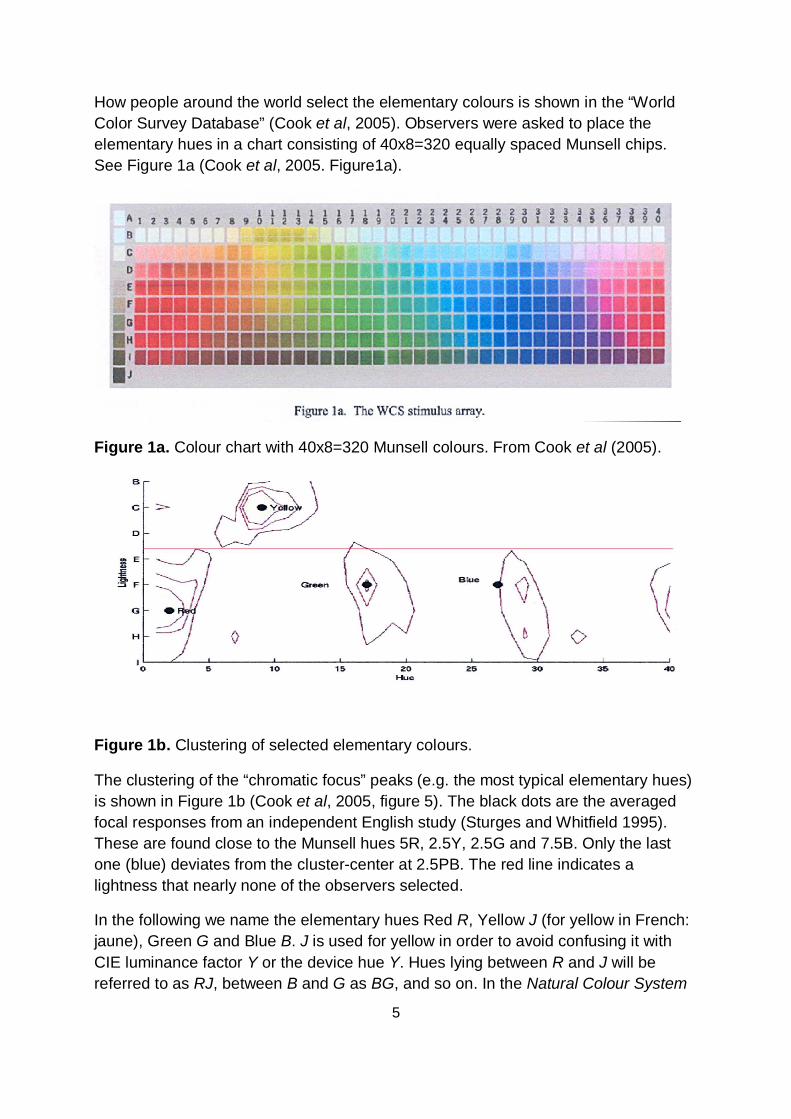
How people around the world select the elementary colours is shown in the “World
Color Survey Database” (Cook et al, 2005). Observers were asked to place the
elementary hues in a chart consisting of 40x8=320 equally spaced Munsell chips.
See Figure 1a (Cook et al, 2005. Figure1a).
Figure 1a. Colour chart with 40x8=320 Munsell colours. From Cook et al (2005).
Figure 1b. Clustering of selected elementary colours.
The clustering of the “chromatic focus” peaks (e.g. the most typical elementary hues)
is shown in Figure 1b (Cook et al, 2005, figure 5). The black dots are the averaged
focal responses from an independent English study (Sturges and Whitfield 1995).
These are found close to the Munsell hues 5R, 2.5Y, 2.5G and 7.5B. Only the last
one (blue) deviates from the cluster-center at 2.5PB. The red line indicates a
lightness that nearly none of the observers selected.
In the following we name the elementary hues Red R, Yellow J (for yellow in French:
jaune), Green G and Blue B. J is used for yellow in order to avoid confusing it with
CIE luminance factor Y or the device hue Y. Hues lying between R and J will be
referred to as RJ, between B and G as BG, and so on. In the Natural Colour System

6
(NCS), 100 steps are used between two elementary hues. Therefore, for example
G50B may be used for a hue angle in the middle between the hue angles of the
elementary hue G and the elementary hue B.
2.2 Device colours
The hue of the device colours depends on the type of imaging device we look at. Up
to six chromatic device colours might be used. These are listed in Table 1.
2.3 Different naming of the concept of elementary hues:
In Norway we say: “A much-loved child have many names”. The same might be said
for the concept of elementary hues. They have been called:
1. Chromatic elementary hues or colours
2. Unique hues
3. Primary hues or colours
4. Focal hues or colours
5. Urfarben
6. Psychologically pure hues or colours, or just pure hues or colours
7. Elementary colours
8. Simple colours
9. Basic colours
10. Perceptual universals
“Simple colours” has been used by Leonardo da Vinci and Miescher (Miescher
1970).
The term elementary hues was chosen by the CIE for this reportership. It is used in
the NCS system and there is an easy translation to any language.
2.4 Achromatic hues
Hering included blackness and whiteness as opponent perceptions (Hering, 1878). In
the CIELAB colour space the origin of the (elementary) hue angles is the achromatic
point in the a*,b* plane. The preferred naming of achromatic colours is listed in
Table 1.
NOTE 4: For real applications the measurement data differ usually up to 5 CIELAB in a* and/or b*, and
independent for White W and Black N. Usually both colours are still accepted as achromatic.
7
3. Colour order systems and elementary hues The selection of the elementary hues by CIE should, in addition to being based on newer data, also use the information contained in previously developed colour order systems. 3.1 The Munsell Renotation System This system is based upon experiments where the observer scales colours uniformly (Newhall et al 1943). In the Munsell System the elementary hues are approximately placed at hue 5R, 5Y, 5G and 5PB (Richter 1996). 3.2 The elementary hue system of Karl Miescher (1948)
The Miescher System pre-dates the NCS. It presents the elementary hues R/G along
the x-axis and Y/B along the orthogonal y-axis, making it a so called symmetrical hue
circle. (K. Richter 1996). The 400 step colour circle of this system was produced by a
special dye process to obtain a highly chromatic hue circle where the luminance of
the samples varied, having dark blue colours and light yellow colours. Coordinates for
the colour samples are given for Source C.
The position of the elementary hues in this highly chromatic hue circle was evaluated
by a group of 24 observers. For R, Y and G any single observer, with normal colour
vision, the positioning of the hues is given with a standard deviation of about 1%
(about 4 degrees of 360 degrees). For the elementary blue the standard deviation
was larger, about 2%.
3.3 The Natural Colour System (NCS)
This well-known Swedish system is based on the opponent theory of Ewald Hering
(Hering 1878). The NCS system is based on experimentally defined elementary
hues, having the four system axes aligned with the elementary hues. Achromatic
colours are scaled according to their whiteness and blackness ratio along the z-axis.
NCS data are published in the Swedish Standard SS 01 91 02:2004. The
development and use of this system is summarized by A. Hård, L. Sivik and G.
Tonnquist (1996)

8
3.4 The four elementary colours selected by the CIE
The CIE has defined four highly chromatic colours as “typical” colours Red R, Yellow
J, Green G, and Blue B for colour rendering purposes. The lightness of these “typical”
colours is therefore high for Yellow J and low for Blue B in accordance with our daily
experience with these hues. This is also typical for the Miescher and NCS hue
circles.
3.5 Selection of elementary hue angles in CIELAB The standardized CIELAB (a*,b*) chroma diagram is chosen for comparison of the
different elementary hue angles found in the systems listed above (ISO 11664-4).
Data for Miescher (1948), the Natural Colour System NCS (1996) and the CIE-test
colours number 9 to 12 of CIE 13.3 are presented below. The CIELAB data of the
colour order system NCS, and the CIE-test colours are available for the CIE standard
illuminant D65.
The Miescher data are available for CIE illuminant C. The CIELAB hue angles for CIE
illuminant C and D65 are very similar because of the high chroma of the samples.
None of the colours in these systems contains fluorescent material.
Figure 2. Elementary hues RJGB of the Miescher (1948) 400-step colour circle.
Figure 2 shows the elementary colours RJGB and the two intermediate colours Cgb
and Mbr of the Miescher colour circle. These are all high-chroma colours of varying
lightness.
9
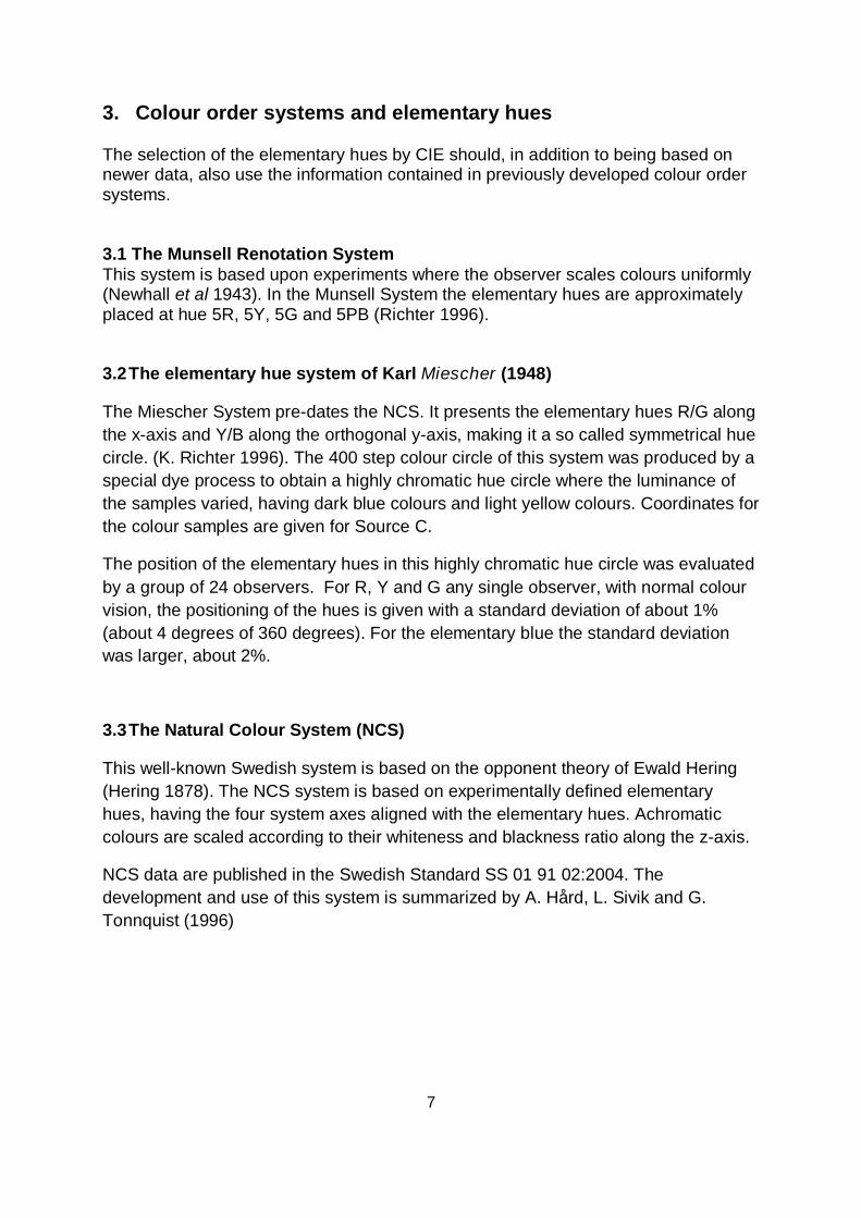
Figure 3. Elementary hues RJGB of the NCS (1996) 400-step colour circle.
Figure 3 shows the elementary colours RJGB and the two intermediate colours Cgb
and Mbr of the NCS colour circle. In the blue area the NCS hue circle is less
chromatic compared to the Miescher hue.
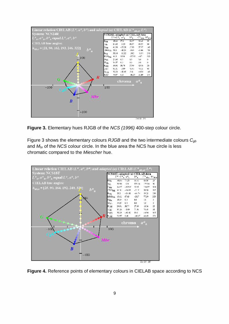
Figure 4. Reference points of elementary colours in CIELAB space according to NCS

10
Figure 4 shows the four extrapolated reference points of the NCS system. These
anchor colours of the NCS system are approximately additionally neither blackish nor
whitish and have the relative blackness n*=0, the relative chroma c*=1 and the
relative whiteness w*=0. The data in figure 4 are taken from the NCS Standard
SS 01 91 02:2004 for the relative blackness n*=0,05 and the relative chromac*=0,95
(not n*=0 and c*=1 since no data are given).
Figure 5: Elementary hues RJGB of CIE-test colours number 9 to 12 according to
CIE 13.3.
Figure 5 shows the elementary colours RJGB of the CIE-test colours number 9 to 12
according to CIE 13.3. The two intermediate colours Cgb and Mbr are calculated by
linear interpolation upon the lines G–B and B–R in the CIELAB space.
3.6 Average hue angles
The hue angles of the high-chroma elementary hues are listed in the figures. If we
calculate an average of Miescher, NCS, and the CIE hue angles given in Figures 2, 4
and 5 we get 26o, 92o, 166o and 270o for R, J, G and B, respectively, which happens
to be quite close to the hue angles of the CIE colours 25o, 92o, 162o and 271o.

11
3.7 Elementary hue planes in CIELAB The figures above only include a single, high-chroma sample for each elementary hue. Ideally, when all samples, having the same hue but different chroma and lightness, are plotted in CIELAB they should end up along the elementary hue lines in the figures above. Figure 6a. All elementary hue samples in the NCS plotted in the CIELAB (a*,b*) diagram. Figure 6a shows all colours samples of the four elementary hue planes in the NCS system. Data-points are taken from Swedish Standard SS 01 91 03 (1982). The R and G hues are close to be ideally placed in planes in CIELAB, but the J and B hues vary in hue angle, with dark samples to the right (close to the b* axis).
NCS Elementary hues in CIELAB
-150
-100
-50
0
50
100
150
-150 -100 -50 0 50 100 150
a*
b*

12
Figure 6b. All samples of hue 5R, 5G, 5Y and 5PB in the Munsell System plotted in the CIELAB (a*,b*) diagram. Figure 6b shows all Munsell samples for 5R, 5G, 5Y and 5PB, including extrapolated
data. For 5R the V5 and V8 data closely follow a straight line, with an angle similar to
the NCS red hues. The V2 data deviate from this line, but most of the V2 values are
extrapolated values, not experimental. For 5Y (yellow) the hue angle is nearly the
same for all samples. For The high-chroma 5G (green) samples deviate from a
straight line. However these are not measured but extrapolated values. For 5PB
(blue) the hue angle for V2 samples deviate from V5 and V8 samples.
Based on the elementary hue data shown in Figures 2 – 6 we may conclude that
there is a general agreement of the elementary hue angles for R, J and G, but a
relatively large variation for the blue hue angle.
4. Experimental definition of elementary hues
4.1 The Jameson and Hurvich type experiments
The classical experiment of Jameson & Hurvich (1955) defined “Chromatic response
functions” by using elementary hue perceptions as criteria. In the experiment they
selected 4 cancellation stimuli, 3 spectral colours which appeared as unique blue,
green and yellow, and 700nm to represent red since elementary red is outside the
spectrum.
For each wavelength of the spectral test stimulus a cancellation stimulus was added
and adjusted until either the redness/greenness was neutralized, or the
Munsell elementary hues in CIELAB. V2, 5 and 8
-150
-100
-50
0
50
100
150
-150 -100 -50 0 50 100 150a*
b*

13
blueness/yellowness was neutralized. The strengths of the four cancellation stimuli
are shown in Figures 7a and 7b. A linear transformation of the CIE Standard
Observer tri-stimulus coordinates can be used to predict the experimental results.
See the solid line in the figures.
Figure 7a Cancellation of redness (open symbols) and greenness (filled symbols).
Figure 7b. Cancellation of yellowness and blueness. (Figures from Larimer et al
1974)
This experiment was later repeated for several luminance levels in order to test
Grassmann’s laws, and if the result could be represented by a linear transformation
of colour matching coordinates. (Larimer et al 1974; Larimer et al1975). They found
that Grassman-type additivity laws could be used for the equilibrium colours of the
red/green opponent process but not for the yellow/blue opponent.
Other researchers found that this non-linearity might be accounted for by assuming
not one but two yellow/blue linear mechanisms (Mausfeld and Niederee 1993,
Chichilnisky and Wandell 1999, Logvinenko 2005). Significant failures in linearity are
observed, but the linear opponent models remain in use in spite of empirical
evidence. The reason is their simplicity. But they can only be used for stimuli of
limited lightness and chroma ranges (Valberg et al 1991).

14
4.2 Observer variation in selecting the elementary hues
Numerous experiments have been done where the observers have to select their
personal elementary hues (EH). If we bundle these results we get a surprisingly large
spread of the selected elementary hues (Kuehni 2001, Kuehni 2004, Abramow 2005,
Kuehni 2005).
A control experiment was done in 2007, with 40 medium-saturated (Chroma 8)
Munsell colours of equal luminance (Value 6). (Hinks et al 2007). The samples were
placed on a light-grey background in a grey box and illuminated with a daylight
simulator at 1424 lx. See Figure 8a. After 2 min. adaptation to the scene the
observers were asked to select their EHs in the usual way: Find the yellow one that is
neither reddish nor greenish, and so on. Each observer repeated the hue selection
after 24 hours.
Figure 8a
Figure 8b
Figure 8a shows the 40 Munsell Chroma 8/Value 6 samples used in the experiment.
In Figure 8b the ranges of selected elementary hues for the 102 observers are
shown, together with the mean hue angles (solid lines).
The experiment verified the large spread of selected elementary colours. See Figure
8b. When the selection of elementary hues was repeated, the same observer
generally selected the same colour samples as before or the neighbouring sample.
This indicates that part of the spread must be due to variation in how elementary
hues are coded in the visual system of the different observers. These variations may
be due to:

15
a) Genetic variations change the absorption spectrum of the cones slightly. In
addition the relative number of L, M and S cones varies markedly between
persons with normal colour vision.
b) The neural network that produce the perception of elementary hues may vary.
c) The adaptation of the eye might vary, making the result vary.
4.3 Other recent experiments
The hue angle spreads in the experiment described above are surprisingly large.
However, other experiments show less variation. In one experiment the colours were
generated on a CRT screen in a dark room (Wuerger et al 2005). A circle of 12
coloured discs of 1.5 degrees diameter was presented on a grey (43 cd/m2)
background. To select elementary red, the observer pointed at the sample appearing
closest to red. 12 new colours were then generated, with hues closer to the selected
one. This procedure was repeated once more to get a precise value that the observer
judged as neither yellow nor blue.
18 observers participated in the experiment. In all, 1616 data-points, obtained for
colours with different chroma and lightness, were recorded. See Figure 9 (Fig. 1 in
Wuerger et al. 2005) where all data-points are displayed in a linear, L, M and S
diagram. Note the different scaling on the x- and y-axis. Here the Smith/Pokorny
cone sensitivities are used. Note that R does not align with the (L-M) axis.
Figure 9. Distribution of 1616 data-points for the elementary hues red, yellow, green
and blue. (After S.M. Wuerger et al 2005)

16
The scatter of the 1616 data points in Figure 9 appears large, but when delta E data
are plotted in the CIELAB space, the variation is about 3 delta E units for the pooled
data. See Figure 10 (Fig. 5 in Wuerger et al 2005).
As in the experiment by Hinks et al (2007), the inter-observer (pooled) data shows
larger spread than the intra-observer (individual) spread. Still, since delta ECIELAB=1 is
roughly the visual threshold, a spread of delta ECIELAB=3 is not more than the allowed
tolerance of colour copiers, according to ISO/IEC 15775.
Figure 10. The mean perceptual errors in delta E*ab units for the four elementary
hues. In addition the mean perceptual errors are shown when the data for elementary
red and green are fitted by a single plane (RG). This implies that different yellow/blue
mechanisms are silenced when the observer perceives a test-colour as elementary
red compared with elementary green.
In another experiment, 185 observers, aged from 18 to 75 years, were tested (under
similar experimental conditions) in order to check if the selection of elementary hues
varied with age (S. Wuerger et al 2009, Fu et al 2009). Their result shows no
significant change of elementary hue selection with age. For all age groups the delta
ECIELAB was less than 3 for nearly 70% of the observers (Private communication with
S. Wuerger).

17
4.4 General comments
The use of aperture colours and high-luminance test colours on darker backgrounds
may change the state of adaptation of the eye and thus influence the results.
Elimination of background will lead to variable adaptation, since the eye then adapts
to the test-sample. The selection of elementary hues is also influenced by the size of
the colour sample. The selection is different for the 2o and the 10o CIE observer
(Nerger et al 1995). For the viewing angles of office documents, only the CIE 2
degree observer is appropriate. The (achromatic) adaptation of the eye will influence
the observer selection of elementary hues. A mean grey background can be applied
for visual displays used at work places. Office documents produced on paper and on
displays both have a standard lightness range between L*=18 and L*=95 according
to ISO 9241-306 and ISO/IEC 15775.
Finally, adapting the eye to different light sources (2800K to 6500K) changes the
elementary hue coordinates (Pridmore 1999).
5 Models
Modeling the perception of colour is approached from two main directions. One may
start with neurophysiologically based studies of how visual information is coded in
neural cells, or by approaching the problem from the perceptional side. A third
approach (often favored by CIE) is to use the tristimulus X, Y, Z transformations of
the cone primaries.
However, no models can predict the correct placement of the elementary hues in the
different colour spaces. Neural coding in the retina and the Lateral Geniculate
Nucleus (LGN) is relatively clearly understood, but less is known about the higher
visual center in the brain (Stoughton 2008). The response of the Parvocellular
neurons in the LGN corresponds poorly with the elementary hues (Valberg 2001). In
the striate cortex the –S+(L+M) from the LGN might be added to the L-M mechanism
from the LGN. De Valois et al have shown that the number of mechanisms containing
the –S+(L+M) signal is doubled in the cortex. (De Valois et al 2000). Based on these
finding one may suggest a solution:
a) if the –S+(L+M) signal from the LGN is added to the L-M cell output then the
resulting response will get an offset from the L-M LGN axis in the unique red
direction.
b) if the –S+(L+M) signal from the LGN is added to the M-L cell output then the
resulting response will get an offset from the M-L LGN axis in the unique green
direction.

18
5.1 Linear models
Earlier, when the three cone spectra L, M and S were unknown, the CIE tri-stimulus
values were often used to model colour vision. The CIELUV is an example of such a
system. Linear models, using linear coded cone sensitivities LMS, are often based on
neural responses for Parvocellular neurons in the LGN. Typical coding types found
here can be expressed as (De Valois 2000):
(L – M), (M-L) and S-(L+M)
Many models use L-M as x-axis and S-(L+M) as y-axis in an opponent cone-
excitation space. However, the weight of the L, M and S components varies
significantly in these cell groups (Tailby 2008). In many experiments with limited
stimulus ranges, linear responses for L, M and S can be used. (De Valois 2000).
When the elementary hues are plotted in such diagrams, the elementary red is often
found close to the L-axis, but the Y, G and B hue angles deviate significantly from the
axes, as shown in figure 11 below ( Webster et al 2000).
Figure 11. Variation in the selection of the elementary hues. From Webster et al
(2000)

19
5.2 Non-linear models
In the linear expressions (L – M) and S – (L + M), shown above, the L, M and S may
be replaced by non-linear responses. In most non-linear models, the cone
sensitivities are replaced with compressing functions. This compressing function can
be a cube root function, as used by CIELAB, or a hyperbolic function (Seim and
Valberg 1986).
For extended ranges of stimulus parameters, only non-linear models can explain
experimental results. When the luminances of spectral lights are varied over a range
of about 4 log-units, then hues change due to the Bezold-Brücke effect. Also when
stimulus luminance increases above a wavelength-dependent value, the chromatic
strength of every hue gets increasingly lower. (Valberg et al1991). This is shown in
Figure 12 for four observers. To explain this result, a non-linear model was used.
Figure 12. The perceptual increase of chroma and variation in hue angle of a
stimulus of constant chromaticity is shown radiating outward as luminance increases.
Further increment of luminance reduces the chroma and continues to change the hue
angle. (From Valberg et al. 1991)
M. Ayama et al (1987) measured the constant hue loci for Elementary red, yellow,
green and blue at 10, 100 and 1000 Td for two observers. Only the hue loci of yellow
at 10 and 1000 Td plotted as straight lines. The other elementary hue loci were
curved.
20
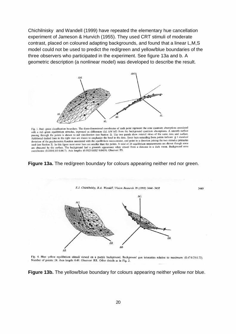
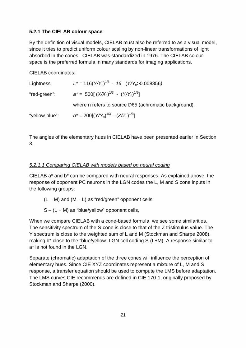
Chichilnisky and Wandell (1999) have repeated the elementary hue cancellation
experiment of Jameson & Hurvich (1955). They used CRT stimuli of moderate
contrast, placed on coloured adapting backgrounds, and found that a linear L,M,S
model could not be used to predict the red/green and yellow/blue boundaries of the
three observers who participated in the experiment. See figure 13a and b. A
geometric description (a nonlinear model) was developed to describe the result.
Figure 13a. The red/green boundary for colours appearing neither red nor green.
Figure 13b. The yellow/blue boundary for colours appearing neither yellow nor blue.
21
5.2.1 The CIELAB colour space
By the definition of visual models, CIELAB must also be referred to as a visual model,
since it tries to predict uniform colour scaling by non-linear transformations of light
absorbed in the cones. CIELAB was standardized in 1976. The CIELAB colour
space is the preferred formula in many standards for imaging applications.
CIELAB coordinates:
Lightness L* = 116(Y/Yn)1/3 - 16 (Y/Yn>0.008856)
“red-green”: a* = 500[ (X/Xn)1/3 - (Y/Yn)
1/3]
where n refers to source D65 (achromatic background).
“yellow-blue”: b* = 200[(Y/Yn)1/3 – (Z/Zn)
1/3]
The angles of the elementary hues in CIELAB have been presented earlier in Section
3.
5.2.1.1 Comparing CIELAB with models based on neural coding
CIELAB a* and b* can be compared with neural responses. As explained above, the
response of opponent PC neurons in the LGN codes the L, M and S cone inputs in
the following groups:
(L – M) and (M – L) as “red/green” opponent cells
S – (L + M) as “blue/yellow” opponent cells,
When we compare CIELAB with a cone-based formula, we see some similarities.
The sensitivity spectrum of the S-cone is close to that of the Z tristimulus value. The
Y spectrum is close to the weighted sum of L and M (Stockman and Sharpe 2008),
making b* close to the “blue/yellow” LGN cell coding S-(L+M). A response similar to
a* is not found in the LGN.
Separate (chromatic) adaptation of the three cones will influence the perception of
elementary hues. Since CIE XYZ coordinates represent a mixture of L, M and S
response, a transfer equation should be used to compute the LMS before adaptation.
The LMS curves CIE recommends are defined in CIE 170-1, originally proposed by
Stockman and Sharpe (2000).

22
5.2.2 Other CIE Colour Appearance Models
A large number of non-linear Colour Appearance Models (CAMs) exists. An overview
of most of them is found in the book of Fairchild (2005). None of these has a
neurophysiologically based description of the elementary hues.
An outline of how device colours are linearized and may be controlled by the use of
elementary hues is presented below.
6. Printing colours In printers the device colours of high chroma are mixed with both black and white to
vary the luminance, and with each other to vary hue. In order to produce a high
chroma hue gamut, three to six device colours are used.
6.1 Linearization of printer-device colours
A device output linearization is fundamental for any colour management application
in imaging (See ISO/IEC TR 19797 and Richter 2008). Usually a grid of 729 = 9x9x9
rgb-input colours is used and the device output colours are measured in CIELAB
coordinates. If the six chromatic device colours X=OYLCVM and Black N and White
W are measured, then DIN 33872 describes a method to calculate the intended
equally spaced 729 output colours both by rgb* and the LAB* coordinates of CIELAB.
Therefore a LAB* to rgb* transition and an rgb* to LAB* transition is known.
L*a*b* - rgb* (LAB* relation)
With the help of the LAB*relation there are three tables of the 729 colours between
the input and output colours:
rgb – rgb* (star relation, based on 8 CIELAB colours)
rgb – rgb*’ (star-dash relation, data rgb*’ of real practical output)
rgb’ – rgb* (dash-star relation, Inverse relation to reach the intended ouput)
Therefore output linearization of any device is reached if a transformation from rgb to
rgb’ (dash) is used for example within the device.
If the input data are equally spaced between 0 and 1 in 9 steps, for example between
Black and White, Black and Red, and White and Red, then for linearized output
systems the three output colours series are equally spaced. This is intended in all
reddish hue planes, including the elementary Red hue plane.

23
6.2 Transfer from device colours to elementary hues
A transfer function must be developed to transfer the device-colours to device-
independent colours based on reproduction of the elementary hues. If the CIE test
colours Red, Yellow, Green, and Blue (RJGB) number 9 to 12 of CIE 13.3 are used
as elementary hues, then for the elementary hues the hue angles are hab = 26, 92,
162, and 272 degrees in CIELAB. From the closest colours in the (tri-dimensional)
set of 9x9x9 colours generated by the device, the device colour for each elementary
hue colour can be computed.
7. Colour displays
7.1 Linearization of display-device colours
A similar method as described for colour printers may be used for displays. One
visual linearization method is given in ISO 9241-306 for work places and for eight
ambient light reflections at the display surface
7.2 Transfer from device colours to elementary hues
A similar method to that described for colour printers may be used.
8. Control of the result Printed control charts may be used as a reference and visually compared with the
output of the device. For displays and projectors a reference display or projector
might be used. Otherwise the output coordinates of the different imaging device can
be measured. There exist 5-, 9-, 17-, 33- step colour series based on 5-step simple
sub-series. Usually observers can evaluate 5-step series on a visual scale between 0
and 1. See for example the 5-step test charts of CIE TC 1-63.
http://www.ps.bam.de/ME23/10L/L23E00NP.PDF
http://www.ps.bam.de/ME05/10L/L05E00NP.PDF
8.2 Illumination used for evaluation of printed colours
For printed images, the relative spectral power distribution of the illumination will
influence the spectral components reflected from the pixels in the image. This,
combined with the adaptation of the eye, will define the colours of the image.
Relevant standard sources are the D65, D50 and source A, the incandescent light-
bulb. The latter may be banned due to its inefficiency and replaced by new, more
efficient light sources, like the LED-based light sources.
24
8.3 Projective devices and ambient illumination
For displays, the ambient illumination will add to that of the displayed image. Care
should be taken to correct for ambient light when colour linearization is performed.
(Thomas et al 2008)
9. Methods for calibrating colour printers and displays using
elementary hues
Two proposals for calibrating colour printers and displays using elementary hues
have been found in the literature:
9.1 Method based on using real observers
This method is presented by D. Karatzas and S. M. Wuerger in the paper:
“Hardware-Independent Colour Calibration Technique” (2008). The idea is to avoid
expensive measurement equipment and complex procedures when calibrating the
elementary hues of an imaging device. This is obtained by the use of a real observer
to define the elementary hues RJGB.
They use a linear model based on light absorptions in the LMS cones, called the HSV
(Hue angle, Saturation, Value) model, to define the elementary colours. Here the
elementary hues of the observer are presented as straight lines in the (L-M), S-(L+M)
diagram.
One advantage of this method is that the observer is always adapted to the real
experimental condition where the device is placed. Since the eye reacts to a highly
complex visual environment a mathematical model will probably not be able to
simulate it.
A short description of their procedure follows:
Task: A Device Under Test (DUT) is compared with a Reference device. On both
devices the observer defines the elementary hue loci as follows:
1. Define achromatic grey through an iterative process
2. Select colours that are neither red nor green
3. Select colours that are neither yellow nor blue
At each trial the HSV coordinates of the selected colours are stored together with the
(linearized) RGB device settings. At least 24 assessments are made by the observer.
4. A device profile is obtained by localizing four planes in the HSV model,
representing each of the elementary hues.
5. A 3x3 transfer matrix is generated that transfers the elementary hue data from
the reference device to the DUT.

25
6. This matrix is then used to transfer any colour on the reference device to the
DUT.
The result can then be visually evaluated by the observer (and other observers) by
comparing the two device images.
Figure 14. A schematic description of the method of Karatzas and Wuerger
9.2 The Relative Elementary Colour System (RECS)
This System is included in a German standard and was developed by K. Richter
(2008). It represents a comprehensive proposal for the application of elementary
hues in image technology. See DIN 33872-1 to -6: http://www.ps.bam.de/D33872-
AE.PDF
The test charts are available at http://www.ps.bam.de/33872E
The charts are found in both digital and analog form in a colour atlas.
The Relative Elementary Colour System uses the standard CIELAB space and a
relative CIELAB space to transfer the CIELAB data of device colours into elementary
hues; see http://www.ps.bam.de/RECS/index.html
The transformations in both directions for the standard and relative CIELAB space
are given in E DIN 33872-1 to -6.

26
The system is developed for calibration of printing and display devices. Linearizing
methods similar to the method given in ISO/IEC TR 19797 are used to make the
output for the 9- and 16-step colour series equally spaced in CIELAB in the
elementary hue planes RJGB and in 12 intermediate hue planes.
9.2.1 Normalization
The device colours White W and Black N and the four elementary colours Red R,
Yellow J, Green G and Blue B are reference points. The relative coordinates of the
RECS are scaled in relation to these reference points. These coordinates are
computed from the standard CIELAB L*, a*, b* coordinates (ISO 11664-4/CIE S 014-
4) for CIE standard illuminant D65 and the CIE 2 degree observer.
9.2.2 Transfer equations
The CIELAB coordinates are transformed into RECS coordinates which show some
similarities with the coordinates of the NCS system. Three colorimetric coordinates
are used to specify the device-produced colours. These are brilliantness i* (equal to 1
minus blackness n*), relative chroma c* and hue angle hab.a (explained below) or
elementary hue u*.
9.2.3 Presentation system
In order to simplify the presentation of surface colours the following normalization
transformation of the CIELAB coordinates was done:
The lightness L* was replaced by relative lightness l* = (L* - L*N)/(L*W – L*N) making
l* vary between 0 and 1.
L*N is the value for the device-black (N for Noir in French) and L*W is the value for
device-white.
The CIELAB coordinates a* and b* are replaced by
a*a = a* - a*N – l*[a*w – a*N]
b*a = b* - b*N – l*[b*w – b*N].
NOTE 7: If the CIELAB data a* and b* are zero for the achromatic colours Black (N) and White (W)
then the adapted (Index a) CIELAB data are equal to the standard CIELAB data.
The last term in these two equations ensures that both a*a and b*a is zero
for both Black N and White W.
From this we can define chroma in adapted CIELAB:
C*ab,a = [a*a2 + b*a
2]1/2

27
The adapted hue angle hab,a can be expressed by
h*ab,a = arctan (b*a / a*a )
The relative chroma c* can then be defined by
c* = C*ab,a/ C*ab,a,M
where M represents maximum chroma of any device for a given hue, and c* varies
between 0 and 1.
The new representation, called the Relative Elementary Colour System (RECS), uses
the coordinates l*, c*, both with values between 0 and 1, and the adapted hue angle
hab,a to represent any surface or display colour. See Note 1.
9.2.4 Elementary hues
The hue angles for the elementary hues are defined by the coordinates of the CIE
Standard colours number 9 to 12, according to CIE 13.3. The hue angles hab in
CIELAB are 26o, 92o, 162o and 272o for the elementary hues R, J, G and B,
respectively.
Figures 15 and 16 contain some equations to calculate the adapted (Index a)
CIELAB coordinates (a*a, b*a) for the standard device systems ORS18 (offset) and
TLS00 (television). See ISO/IEC 15775.
NOTE 8: For the definition of brilliantness i*, blackness n*, elementary hue text u* and others see the
documents of the standard series DIN 33872.

28
Figure 15. Device hues Y, L, C, V, M and O and elementary hues R, J, G and B for
offset system ORS18. Hue angles for device (d) and elementary hues (e) are
included in the figure.
For the device system ORS18 (Offset) both the coordinates (a*N, b*N) of Black N and
(a*W, b*W) of White W are different from zero, but the adapted coordinates are equal
to zero.
Figure 16. Device and elementary hues for television display system TLS00. (See
explanation of data in Figure 15).
For the device system TLS00 (Television), both the coordinates (a*N, b*N) of Black N
and (a*W, b*W) of White W are equal to zero, and therefore it is always valid that (a*,
b*) = (a*a, b*a).
29
In Figures 15 and 16 the colours with the hue angles of the CIE-test colours number
9 to 12 are compared with the six device colours for the standard offset print system
ORS18 and a standard monitor system TLS00 according to ISO/IEC 15775: 1999.
The two colours Cgb = G50B and Mbr = B50R, with a hue angle in the middle between
G and B, and between B and R are added in the figures.
10. Proposals People react more strongly to errors in hue reproduction (hue shifts) compared to errors in lightness and chroma reproduction (Taplin 2004). In addition, many prefer the use of elementary hues when they evaluate a test chart reproduction, and they would like to avoid the variability found when device colours are used in the reproduction. 10.1 Selection of elementary hue angles The variation of elementary hue angles in the literature is due to individual variations as well as to different experimental conditions. While some experimenters get surprisingly large variation in observer hue angles, others get less variation. Data from the Colour Order Systems (Figure 2 – 5) shows much less variation, except for elementary blue. This experimental divergence is probably partly due to different experimental conditions, and this should be clarified further by the CIE. Experimental conditions, typical for evaluation of imaging device outputs, should be preferred.
10.1.1 Proposal: A further study of the selection of elementary hue angles should be done by
the CIE to analyze the scatter of experimental defined angles. The results
should appear in a CIE Technical Report.
The average of Miescher, NCS, and the CIE elementary hue angles is quite close to the hue angles of the CIE colours number 9 to 12 (See 3.6 above). The hue angles of the CIE colours can be used as preliminary values. 10.2 Modification of “Method based on using real observers”
See 9.1: “Method based on using real observers.”This method is presented byKaratzas and Wuerger in the paper: “Hardware-Independent Colour Calibration Technique” (2007). The advantage of their method is its simplicity.

30
However, if CIE decide to consider this approach, they should also modify it. An obvious way of doing this is to use the method presented by Jameson and Hurvich (1955). They replaced the experimental observers with the CIE Standard Observer. The same substitution can be done with the real observers used by Karatzas and Wuerger. 10.2.1 Proposal: The modified method of Karatzas and Wuerger should be considered as a possible basis for a CIE Technical Report. 10.3 The Relative Elementary Colorimetric System (RECS)
This system fulfills most of the criteria for a CIE-based method for calibration of
imaging devices. It is based on the (nonlinear) CIELAB space, and it includes test
charts.
10.3.1 Proposal: The Relative Elementary Colorimetric System of Richter should be considered
as a possible basis for a CIE Technical Report
NOTE 9: The reflection factors of the CIE-test colours and reference samples by different sources are
available. They can be used for many additional visual experiments. Colour constancy experiments
suggests that the CIE-test colours remain the property “Elementary Hue” under different illuminants,
for example the image technology illuminants D65 and D50.

31
Acknowledgments
Figures 2-5 were kindly produced for the report by Klaus Richter. He also helped me by explaining his Relative Elementary Colour System (RECS). Arne Valberg gave me important information about elementary colours, including the Miescher System. I am also grateful for information I received from Rolf Kuehni and Sophie Wuerger about their experiments.

32
References
I. Abramov and J. Gordon, "Seeing Elementary hues," J. Opt. Soc. Am. A 22, 2143-
2153 (2005)
C. F. Andersen, J. Y. Hardeberg, “Colorimetric characterization of digital cameras
preserving hue planes”, 13.th Color Imaging Conference, Scottsdale, Arizona (2005).
M. Ayama, T. Nakatsue, and P. K. Kaiser, "Constant hue loci of unique and binary
balanced hues at 10, 100, and 1000 Td," J. Opt. Soc. Am. A 4, 1136-1144 (1987)
E. J. Chichilnisky, B. A. Wandell, “Trichromatic opponent color classification”, Vis.
Res. 39, 3444-3458 (1999).
R. S. Cook, P. Kay, T. Regier, “Handbook of Categorisation in the Cognitive
Sciences”, page 1: The World Color Survey Database: History and Use” ( 2005)
R. L. De Valois, N. P. Cottaris, S. D. Elfar, L. E. Mahon and J. A. Wilson, “Some
transformations of color information from LGN to striate cortex”, Proc. Natl. Acad. Sci.
USA, 97 (9), pp 4997-5002. (2000).
M.D. Fairchild “Color Appearance Models”, Second Edition, USA John Wiley & Sons,
Ltd (2005)
C. Fu, K.Xiao, D. Karatzas and S. Wuerger, “Changes in colour perception across the
life span”. To be presented at the AIC in Sidney (2009).
A. Hård, L. Sivik and G. Tonnquist ,“NCS, Natural Color System – from Concept to
Research and Applications”, Color Res. Appl., 21,No 3, p180-205 (1996)
E. Hering, “Zur Lehre vom Lichtsinne”, C. Gerold’s Son, Vienna. Or: “Grundzüge der
Lehre vom Lichtsinn”, (Springer, 1905-1911)
D. Hinks, L. M. Cárdenas, R. G. Kuehni, R. Shamey, “Unique-hue stimulus selection
using Munsell color chips”, J. Opt. Soc. Am., 24(10),(2007)
D. Jameson and L. M. Hurvich (1955), “Some quantitative aspects of an opponent-
colors theory. I. Chromatic responses and spectral saturation.”, J. Opt. Soc. Am., 45,
546.
T. Jean-Baptiste, J. Y. Hardeberg, I. Foucherot, P. Gouton, ”The PVLC Display Color
Characterization Model Revisited”, Color Res. Appl., 33(6), 449-460 (2008).
D. Karatzas and S. M. Wuerger, “A hardware-Independent Colour Calibration
Technique”, Annals of the BMVA Vol. 2007, No. 3, pp 1-10 (2007)
R. G. Kuehni, “Focal color Variability and Unique Hue Stimulus Variability”. Journal of
Cognition and Culture, 5 (2005)

33
R. G. Kuehni, “Determination of unique hues using Munsell color chips”, Color Res.
Appl., 26(1), 61-66 (2001).
R. G. Kuehni, “Variability of unique hue selection: a surprising phenomenon”, Color
Res. Appl. 29, 158-162 (2004)
J. Larimer, D. H. Krantz, C. M. Cicerone, ”Opponent process additivity – I. Red/Green
equilibria”, Vis. Res. 14, pp1127-1140(1974).
J. Larimer, D. H. Krantz, C. M. Cicerone, ”Opponent process additivity – II.
Yellow/Blue equilibria and nonlinear models”, Vis. Res. 15, pp723-731(1975).
A. D. Logvinenko, S. J. Hutchinson, “One blue channel or two?”, Perception, 34,
p921-925 (2005)
R. Mausfeld, R. Niederée, “An inquiry into relational concepts of colour, based on incremental principles of colour coding for minimal relational stimuli”, Perception, 22, p427-468 (1993) K. Miescher, “Neuermittelung der Urfarben und deren Bedeutung für die Farbordnung”, Helv. Physiol. Acta 6, C12-C13 (1948) K. Miescher, “Leonardo da Vinci, Göthe und das Problem der einfachen und zusammengesetzten Farben”, Die Farbe 19, 269-276 (1970) N. Moroney, “A Radial Sampling of the OSA Uniform Color Scales”, Proceedings of
the 11th IS&T/SID color imaging conference, (2003):
www.hpl.hp.com/personal/Natham_Moroney/osa-radial-560.dat
J. L. Nerger, Vicki J. Volbrecht, and Corey J. Ayde, "Unique hue judgments as a
function of test size in the fovea and at 20-deg temporal eccentricity," J. Opt. Soc.
Am. A 12, 1225-1232 (1995)
S. M. Newhall, D. Nickerson, D. B. Judd, “Final report of the O.S.A. subcommittee on
spacing of the Munsell colors”, J. Opt. Soc. Am. 33, 385 (1943)
R. W. Pridmore, “Unique and binary hues as functions of luminance and illuminant
color temperature, and relations with invariant hues”, Vision Research, Volume 39,
Issue 23, Pages 3892-3908 (1999)
K. Richter, “Computergrafik und Farbmetrik”, VDE-Verlag GMBH, Berlin (1996)
K. Richter, The Relative Colorimetric System (RCS) based on device and elementary
colors. Proceedings Report, Colour – Effects & Affects, Interim Meeting of the
International Colour Association (AIC), paper N156, 4 pages, Stockholm 2008

34
K. Richter, Colour management reference circle: Scan – File – Print – Scan using a
CIELAB camera and standard offset printing, pages 204-208, Proceedings of the CIE
expert symposium on “Advances in Photometry and Colorimetry”, Turin, CIE
x033:2008
B. A. C. Saunders and J. van Brakel, “Are there nontrivial constrains on colour
categorization?”, Behavioral and Brain Sciences, 20(2), p 167 (1997).
B. E. Schefrin and J. S. Werner, ”Loci of spectral unique hues throughout the life
span”, J. Opt. Soc. Am. 7(2), 305-311 (1990)
T. Seim, A. Valberg, “Toward a Uniform Color Space: A better formula to Describe
the Munsell and OSA Scales”, Color Res. Appl. 11(1), 11-23 (1986)
Stockman, A., Jägle, H., Pirzer, M. and Sharpe, L. T.: “The dependence of luminous
efficiency on chromatic adaptation”, Journal of Vision 8(16), 1-26. (2008)
J. Sturges, T. W. A. Whitfield, “Locating the basic colours in the Munsell space”,
Color Res. Appl. 20, 364-376 (1995)
B M. Stoughton and B. R. Conway, “Neural basis for unique hues”, Current Biology,
18, no 16, page R698-699 (2008).
C. Tailby, S. G. Solomon, P. Lennie, ””Functional Asymmetries in Visual Pathways
Carrying S-Cone Signal in Macaque”, Journ. Neuroscience, 28(15),4078-4087 (2008)
L. A. Taplin, G. M. Johnson, “When Good Hues Go Bad”, CGIV Second European
Conference in Colour in Graphics, Imaging and Vision(2004)
J. B. Thomas, J.Y. Hardeberg, I. Foucherot, P. Gouton, “The PLVC Display Color
Characterization Model Revisited”, Color Res. Appl. 33(6), 449-460 (2008)
A Valberg, B. Lange-Malecki and T. Seim, “Colour changes as function of luminance
contrast”, Perception, 20, p655-668 (1991).
A. Valberg, “Elementary hues: an old problem for a new generation”. Vision
Research, 41, 1645 – 1657(2001).
M. A. Webster, E. Miyahara, G. Malkoc and V. E. Raker. “Variations in normal color
vision. II. Unique hues”. J. Opt. Soc. Am. (2000).
S. M. Wuerger, P. Atkinson and S. Cropper, “The cone input to the unique-hue
mechanisms”, Vision Research, 45, p3210-3223 (2005).
S. M. Wuerger,C. Fu, K. Xiao and D. Karatzas, “Colour-opponent mechanisms are
not affected by sensitivity changes across the life span”. To be presented at the AIC
in Sidney (2009).

35
Standards and recommendations
Swedish Standard SS 01 91 03, CIE tristimulus values and chromatcity co-ordinates
for the colour samples in SS 01 91 02. Edition 1982 for Source C and edition 1996
for Source D65.
ISO/IEC 15775, Information technology—Office machines—Method of specifying image reproduction of colour copying machines by analog test charts—Realisation and application
ISO/IEC 19797:2004, Information technology -- Office machines -- Device output of
16 colour scales, output linearization method (LM) and specification of the
reproduction properties
ISO/IEC 24705:2005, Information technology -- Office machines -- Machines for
colour image reproduction -- Method of specifying image reproduction of colour
devices by digital and analog test charts
ISO 9241-306:2008, Ergonomics of human-system interaction -- Part 306: Field
assessment methods for electronic visual displays
ISO 11664-4/CIE 1976 L*a*b* Colour space
ISO TC159/SC4/WG2: Visual Display Requirements
CIE 13.3-1995: Method of measuring and specifying colour rendering of light sources
New edition
CIE 170-1:2006: Fundamental chromaticity diagram with physiological axes - Part 1
CIE X030:2006 p. 139-144, Klaus Richter, Device dependent linear relative CIELAB data lab* and colorimetric data for corresponding colour input and output on monitors and printers, CIE Symposium, 75 years colorimetric observer, Ottawa/Canada DIN 33872:2007 Information technology - Office machines - Method of specifying
relative colour reproduction with YES/NO criteria
W. W. Coblentz and W. B. Emerson, Relative sensibility of the average eye to light of
different colors and some practical applications to radiation problems, Bull. Bur.
Stand. 14, 167-236 (1918).


![COMPUTER ORGANIZATION & ARCHITECTURE · mov r3, h r3 m [h] add r3, g r3 r3+m [g] div r1, r3 r1 r1/r3 mov x, r1 m[x] r1 page 4 of 16 knreddy computer organization and architecture](https://img.pdfslide.us/doc/110x75/6144b5c334130627ed50859a/computer-organization-architecture-mov-r3-h-r3-m-h-add-r3-g-r3-r3m-g.jpg)


![lr V≤ Xmg]m{Y - samarthramdas400.in/cite>MaUHù_cr](https://img.pdfslide.us/doc/110x75/5af7c1867f8b9a44658b7d2d/lr-v-xmgmy-.jpg)