Embed Size (px)
Citation preview
CID~
II
-41
KLL
.11
UNITED STATES AIR FORCE,~1I AIR UNIVERSITY
AIR FORCE INSTITUTE OF TECHNOLOGYWright-Patterson Air Forc* Base,OhIai
or Public x un Oprve
is litniledsoo z
7908203 0971
~AAUG L4 1979 f
THE USE OF THE MAURER FACTOR FORESTIMATING~ THE COST OF A TURBlINE
Eli ENGINE IN THE EARLY STAGESOF DEVELOPMENT
Charles W. Barrett, Jr.,, Ca tain, USAFMichael J. Koenig, Capta n, USAF
LSSR 1.9-79A
I, I d
•'-aul - rnIitbnl 'tM~fkfliu ~ .A ~ a
The contents of the document are technically accurate, and
Sno sensitive items, detrimental ideas, or deleteriousinformation are contained therein. Furthermore, the viewsexpressed in the document are those of the author(s) and donot necessarily reflect the views of the School of Systemsand Logistics, the Air University, the Air Training Command,the United States Air Force, or the Department of Defense.
L?
Vt
NI
.1 ~ -
USAF SL 75-Z2B AFTT Control mnber-- ---
r AFIT RESEARCH ASSESM"4TThe purpose of this questionnaire is to determine the I _ntial for currentand future applications of AFIT thesis research. Please return completed
1. Did this research contribute to a current Air Force project?
a. Yes b. No
2. Do you believe this research topic is significant enough that it wouldhave been researched (or contracted) by your organization or another agencyif AFIT had not researched it?
a. Yes b. No
3. The benefits of ARZT research can often be expressed by the equivalentvalue that your agency received by virtue of AFIT performing the research.Can you estimate what this research would have cost if it had beenaccMlished tunder contract or if it had been done in-house in terms of man-power and/or dollars?
a. Man-years ....... $ . (Contract).
b. Man-years __,_$ _ ,,, (In-house).
4. Often it is not possible to attach equivalent dollar values to research,although the results of the research may, in fact, be important. Whether ornot ydu were able to establish an equivalent value for this research (3 above),what is your estimate of its significance?
a. Highly b. Significant c. Slightly d. Of NoSignificant Significant Significance
S. Couemts:
Nmne Ea Crade Position
Oraizto rocation '4.4'•:,. . • . • j !•. .. ... _ ,•.. _ _ .. •, _ . - .• - -- , _ - - - - :.,.;•,.:!T - ,• , . . . . . ..
MICUSARVI
BUSINESS REPLY MAIL
PWAGS~ WAL if PAID aY AOOR4USlU___________
A.FIT/LSH (Thesis Feedback)W~±g~-Paa~~A.FB 09 41433 ________
SECURITY CL.ASSIF'ICATION OF' THIS PAGE ("o Dole Entered)
00 COERACO
-HE E OF THE-ZAURER. ACTOR
~N THE gARLY _SiFAES OF D)2VEOPMVENT.N AO I
111-CONRACT OR 61ANT NUM11111(oJ
k'i Charles W. /arrett, Jr ,Captain, USAFSI Michael J. aoenig a , USAF
91 1091119AMINO ORGANIZATION NAM9 AND ADORESS to oMGRAM0EkNIMENT, PROJECT, TASK(
Air Force Institute of Technology (AFIT/ ARIA & WORX UNIT NUMSERS
LSG) Air Training ComnmandWright-Patterson AF, OHIO
I.CONTROI,.I.ING OPFICS, NAME AND -DDES /1 Jun7914. MONITORIN Ad NC N i&j&Afli1 diferent from Controlling Ofi~e) Is. 11E1CURITYw CL.ASS. eel this revert) ;
UNCLASSIFIEDIle, IffaustapI E ATI ON/ 55W t Abi N a
ig. DIP1T111114TION STATEMEINT (*I thi. Report)
Approved for public releasee distribution unlimitedý
A 1:71". P . '1' .7, DISTRIBUTION IT ATEMEN (at the abstract entered In Block 20, It differmnt from, Roeor()
Statement Ai A p~ov-ed--for, 'Pu'b'j.2i 1 steaie -Di..s jUto
IS. SUPPLEMENTARY NOTES
11. KE, WORDS (Continuo on toverso side it uecesseary and Identify by. block number)
Turbine EnginesCost Eati~mationMaurer FactorModelsLearning Curve
20. AGITRACT (Continue on reveres side It necessary and identify by block number)
F 147 EDITION 0OP 1 NOV 111 52 ONSOLETE
SECURITY C. Alai IPcATION OR THIS PiaGE (ften r " ee).. ... ...
IRCURITY CLASSIFICATION OF THIS PAGOU(WPhwi Data EnEli'.d)
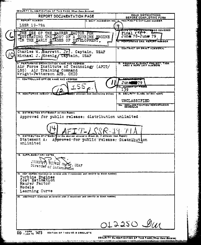
Military managbris are faced with increasing systems costs, ;n~earea where this increasing cost is especially true is in theacquisition of aircraft weaponf systems. A driving factor in theaircraft cost is the turbine engine# and therefore acquisitionmanagers ha~ve been taskced with developing cost estimating methods
C' that will more accurately predict turbine engine cost. Atpresent, several ýarametrio costing models available are brieflydiscussed in this report. However, the primary objective of thisreport, is to evaluate a costing technique used extensively by the
V Navy--the Maurer Factor (MP) technique. The MF technique is aparametric costing technique based on the materials in a turbineengine. The report includes the followingi (a) a detaileddescription Ole the MP technique; (b) a validation of the MFtechnique; (c) the development of an estimated MF (EMF) mL'odelusing engine performance parameters; and (d) statistical analysisand validation of the EM? models.~
sacupiry CLASSIFICATION OR r~4is PA4se(wPan BeraWtared)
~~~~~~ L.. F...,
LSSR 19-79A
THE USE OF THE MAURER FACTOR FOR ESTIMATING
THE COST OF A TURBINE ENGINE IN THE
EARLY STAGES OF DEVELOPMENT
Itis
A Thesis
Presented to the Faculty of the School of Systems and Logistics
of the Air Force Institute of Technology
Air University
In Partial Fulfillment of the Requirements for the
Degree of Master of Science in Logistics Management
By
Charles W. Barrett, Jr., BA Michael J. Koenig, BACaptain, USAF Captain, USAF
June 1979
Approved for public release;distribution unlimited
I. ....... .. A.
This thesis, written by
Captain Charles W. Barrett, Jr.
and
Captain Michael J. Koenig
has been accepted by the undersigned on behalf of the facultyof the School of Systems and Logistics in partial fulfillmentof the requirements for the degrees of
MASTER OF SCIENCE IN LOGISTICS MANAGEMENT(Captain Charles W. Barrett, Jr.)
MASTER OF SCIENCE IN LOGISTICS MANAGEMENT (CONTRACTINGAND ACQUISITION MANAGEMENT MAJOR)
(Captain Michael J. Koenig)
DATE, 6 June 1979
COMW E CHAIRMAN
UP
/,
ACKNOWLEDG=ENTS
The authors wish to express their gratitude for the
valuable information provided to them by the Maurer Factor
sponsor Mr. Pressman and specifically his experts at the
Naval Air Development Center, Warminster, PA--Mr. Finizie
and Mr. Friedman. We extend our appreciation for the long
hours and extensive research that Mr. Richard McNally of
the Propulsion Branch at Wright-Patterson AFB conducted to
provide us with extremely valuable information for inclusionin this report, Furthermore, we wish to thank Major Leslie
Zambo, our faculty advisor, for his expert advice for the
successful completion of this report. Finally, we express
our thankfulness for such loving and supporting wives
without whom this report would not have been possible,
iiii
ill 1V
.11,' -. '*V.V. QJ .~-. -, .,,I!:. .' VV'I' -C VP
'I!TABLE OF CONTENTS
Page
LIST OF TABLES . . . . . . . . . . . . . . . . .viii
LIST OF FIGURES . . . .......... ..... . X
Chapter
1. INTRODUCTION . . . . . . . . . . . . . . . . . . 1
Background
Problem Statement . . . . . . . , . . . , . .
Justification . .. ,. . ... . . . 2
"2. LITERATURE REVIEW , , , . , . , , . . . 6
Cost Estimation , ... ... , . 6Engineering-accounting 6
Statistical analysis 7
Linear regression . . 8 . , ., , , , . 8
Turbine Engine CostEstimation * ., . .. , , , . , to
Rand model . . , A , , * * , . .#
Grumman model a, , .. .. .. . 14
"Mullineaux and Yanke model , . . . . , . , 15
Maurer factor . . . . . . . a . . a . 17
The Learning Curve , .#. a .# , .. . * o ,a& 24
Objectives A . . . .A . .. . .A . . 25
Research Questions , , . A,, ... A. 26
Research Hypothesis a S A A A A A . , A A , 26
Summary 26
iv iv .U
Chapter Page
3. RESEARCH METHODOLOGY .. . . . . ....... . 28Overview £ * S a . . a. . . .. . . . .. . 28
Variables of Interest ... .. .a. 28
Justification of VariableSelection . a a a . , a . . a . , , .. . 28
Selection of IndependentVariables . . . . . . . . a . a . a a . a a 30
Method of Data Collection . a £ . , . . 30
Population and SampleDescription . a a a a a a , . • a a . a . a 33
Model Justification 35
Model Development ... a a a a a a a a a 36
Regression Analysis 36
Validation Process ... a a a a a a . .a 37
The Maurer Factor technique . a a a a a a 37
Estimated Maurer Factor model validation a 37
Selection test criterion , a , a a . a a a 38
Summary List ofLimitations a a a . .a a.. . . . a . a a 38
Summary List ofAssumptions 36. a a a a a a a a . a. . a 3
1.1 4. DATA ANALYSIS AND FINDINGS . a . a . a .. a.. 40
Introduction # 40
Maurer Factor Cost EstimatingTechnique a , . a a a a a a a . . a a a a , 40
Learning curve cost adjustment . . a . . . . 40
Profit and General and Administrative costadjustments . . .a .a .a. . .. a 41
V .
Chapter Page
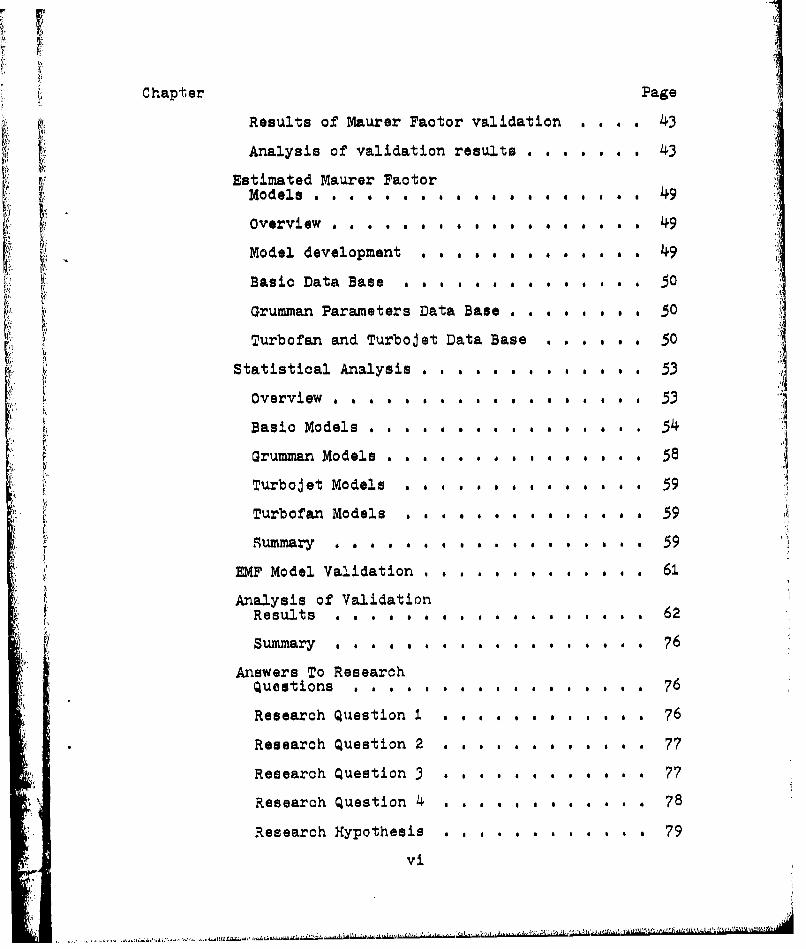
Results of Maurer Factor validation . . . . 43
Analysis of validation results . . . . . . . 43
Estimated Maurer FactorModel~s . . a * a a a a a a a a a a a a a a 49
overview . . . . . . . . . a . . a a . a . 49
Model development aaaaaaa aa.aa49
Basic Data Base . a a .aa .. .. 50k •i• Grumman Parameters Data Base 3 a a a a . , a 50
Turbofan and Turbojet Data Base s a . a a . 50
Statistical Analysis is.. . .a. . 53
Overview . a a a a a a a a , a , a a a a a 53
Basic Models . . . . . . . . . . . . . . . 54
Grumman Model s .... . . . .. . . . . . . 58
Turbojet Models . . , .a .. , 59
Turbofan Models . . . , 1, ,a 59
Summary a a a . . . a a . . . . a . a a a a 59
EMF Model Validation .. , .. , , . 61
Analysis of ValidationResults a a a a a a , a . a a . .a. a. , 62
Summary a a a a a a a a 76
Answers To ResearchQuestions , a a . , a a a a a a , a a a a a 76
Research Question 1,.,.., a,, . 76
Research Question 2 # , a a at a a a a 77
Research Question 3 . a a a . . a a a a a a 77
Research Question 4 a & aa a aa a .. 78
Research Hypothesis a a a .. a ... a a a 79
vi
Chapter Page
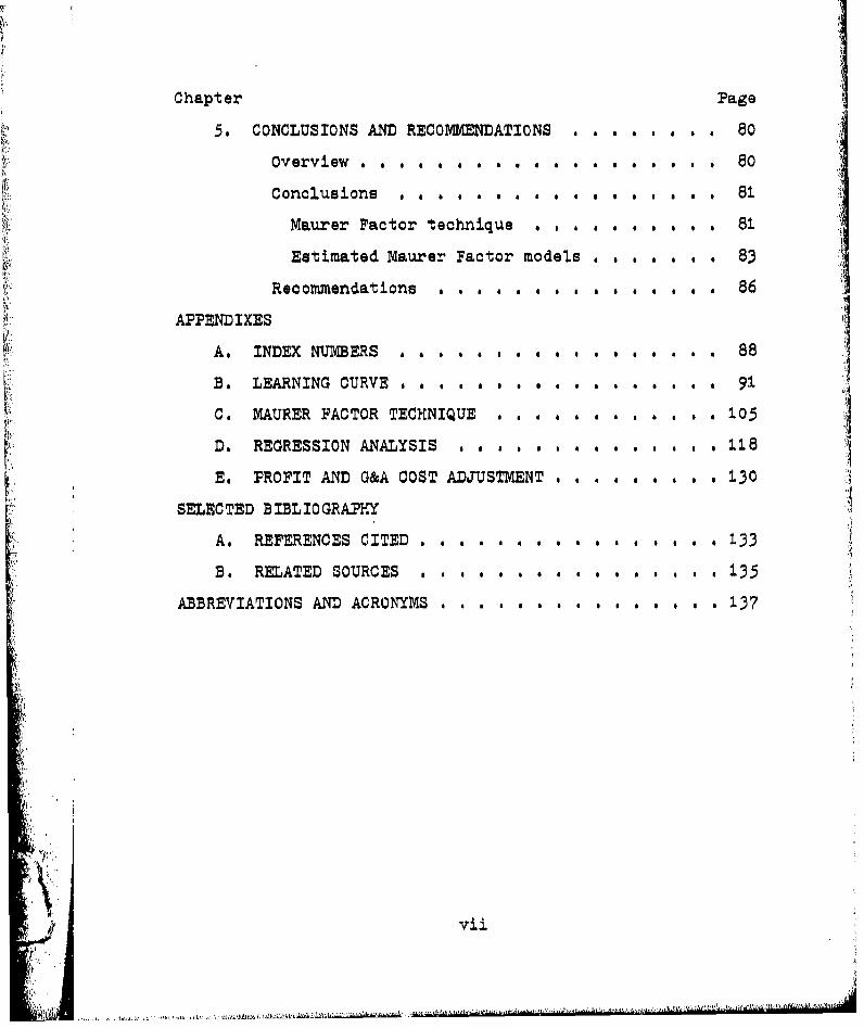
5. CONCLUSIONS AND RECOMMHENDATIONS , a .. ,. .80
Overview , . . . . . • .. • . . . . .. . . 80 +
Conclusions 81
Maurer Factor technique . a a . . . , . 81
Estimated Maurer Factor models . . . . . . . 83
Recommendations . . . . . . . , . a a a a 86
APPENDIXES
A. INDEX NUMBERS . . . . . . . . . . 88
B. LEARNING CURVE . . . a a , . . . a a . . a 91
C. MAURER FACTOR TECHNIQUE . a a . . .. . . . 105
D. REGRESSION ANALYSIS o . a a a a a . . a . , . 118
E. PROFIT AND G&A COST ADJUSTMENT . . . . . . . . . 130
SELECTED BIBLIOGRAPHY
A. REFERENCES CITED .... . .... . . . . . . . 133
B. RELATED SOURCES . a. . a . . .a a a 135
ABBREVIATIONS AND ACRONYMS .. .. .. . . .a . ... . 137
'pi
*1.,- vjii- r . . ".,I-.
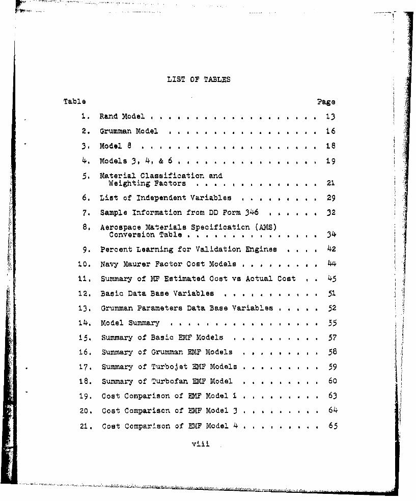
LIST OF TABLES
Table Page
1. Rand Model . . . . . . . . ,. . . a 13
2. Grumman Model . a a . . 6 a g1 16
3. Model 8 . . . . . . . . .a g . a a a a a a .a 1.8
4. Models 3, 4, & 6 a a . a a a a . . a a a a 19
5. Material Classification andWeighting Factors . ..... a . a 1 g . 21
6. List of Independent Variables . . . a . a . . . 29
7. Sample Information from DD Form 346 , . . a . 32
8. Aerospace Materials Specification (AMS)Conversion Table a . , a . a a sagaa 34
9. Percent Learning for Validation Engines a a a . 42
10. Navy Maurer Factor Cost Models . . . . . . a 44
11. Summary of MF Estimated Cost vs Actual Cost a a 45
12. Basic Data Base Variables a a . a . . a a a a 51.
13. Grumman Parameters Data Base Variables . a a . a 52
14. Model Summary . . . . . . a . . a . . . . . . . 55
15. Summary of Basic EMF Models . .a . . . .a a . 57
16. Summary of Grumman EMF Models . . . a . . * . 58
17. Summary of Turbojet EMF Models a a . .a. . . . . 59
18. Summary of Turbofan EMF Model , , a a a a a a a 60
19. Cost Comparison of EMF Model I . . . . . . . . . 63
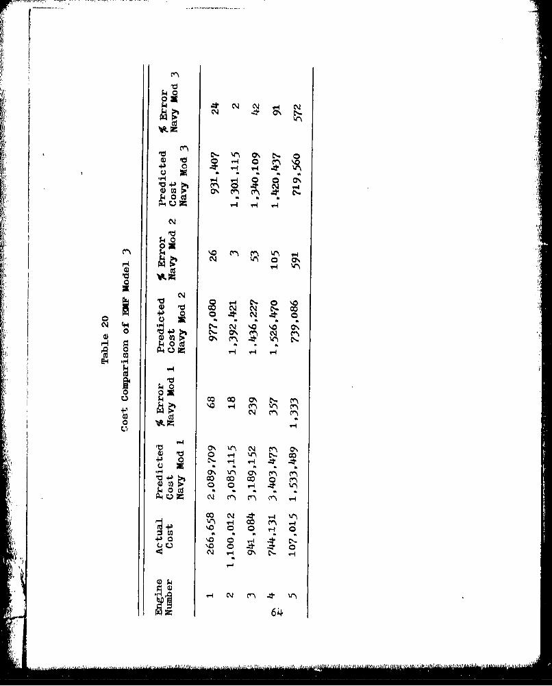
20. Cost Comparison of EMF Model 3 . . . .a. . . . . 64
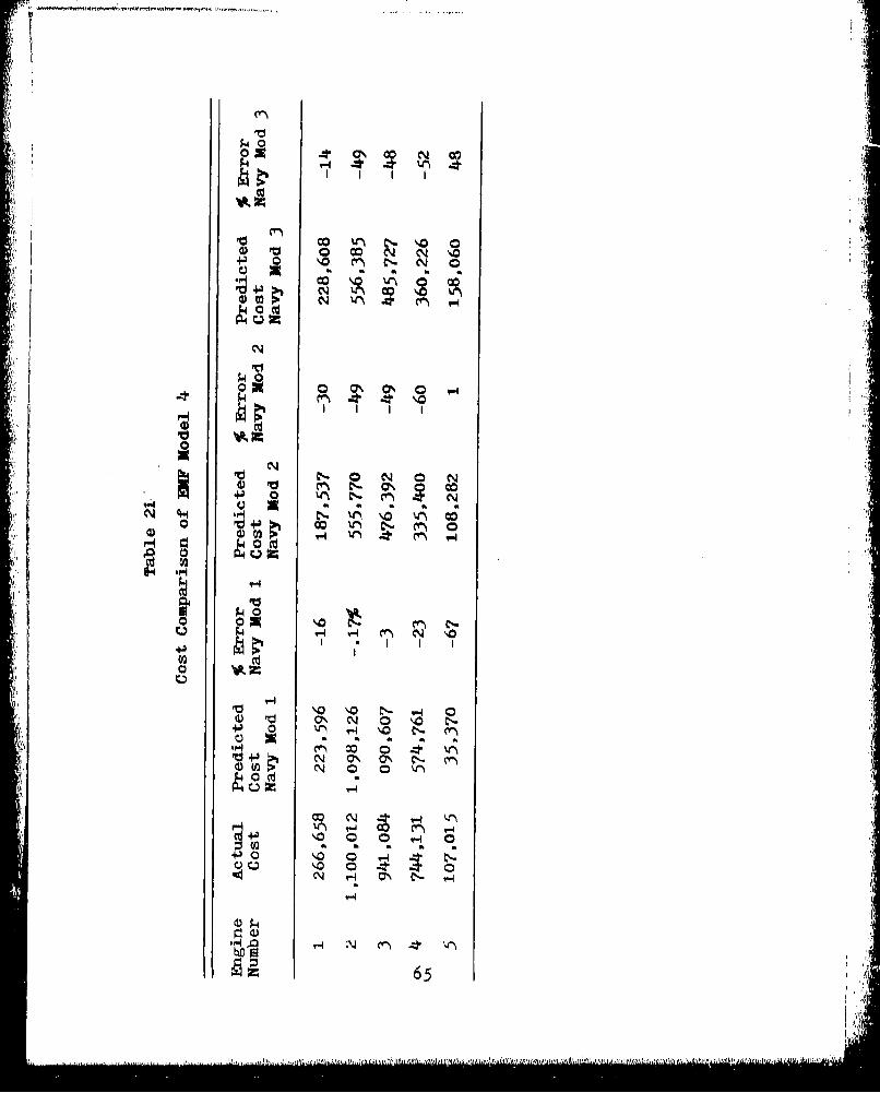
21. Cost Comparison of EMF Model 4 . a . a . . . . a 65
viii
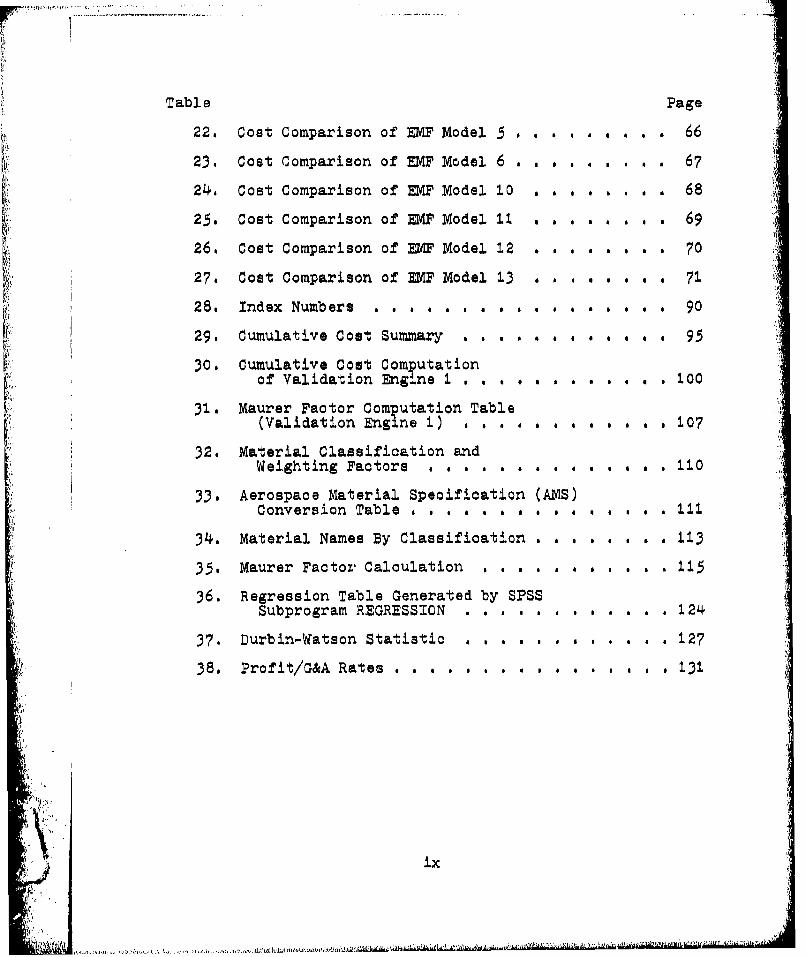
Table Page
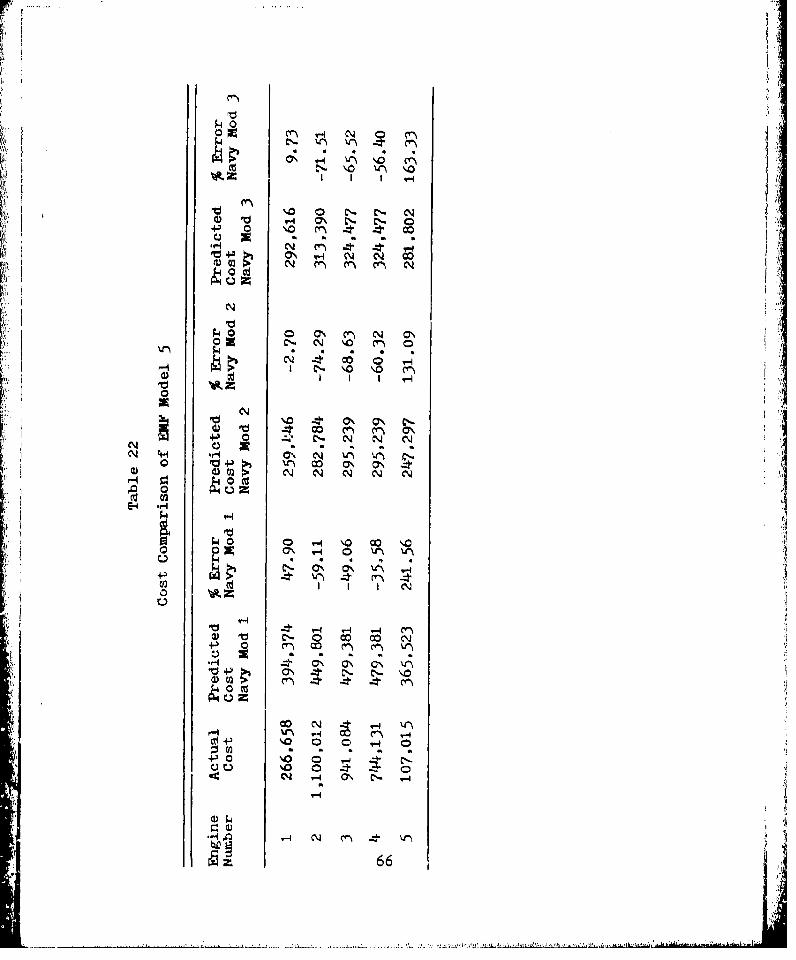
22. Cost Comparison of EIF Model 5 . . . . . . . . . 66
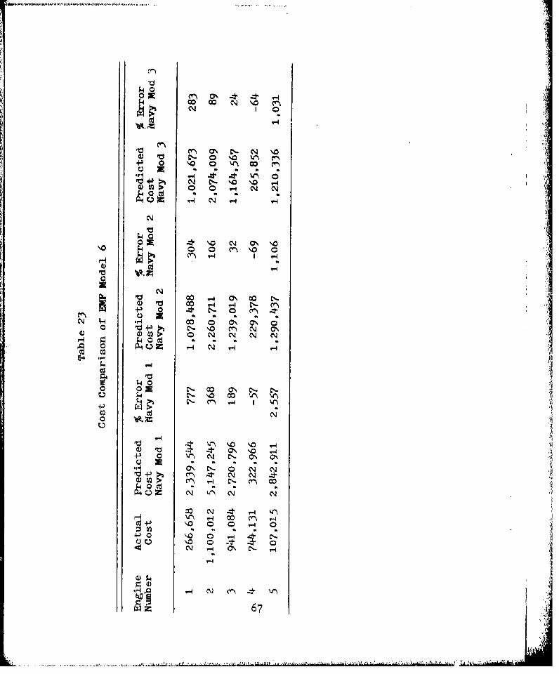
23. Cost Comparison of EMF Model 6 . . . . . . .. . 67
24. Cost Comparison of EMF Model 10 . . a .a. . . . 68
25. Cost Comparison of W4F Model 11 . . . . . .a . 69
26. Cost Comparison of EMF Model 12 . . . . . . . . 70
27. Cost Comparison of EMF Model 13 . . . . . . 71
28. Index Numbers a a a.. .a.a a .a 90
29. Cumulative Cost Summary ..... . . . . , . . 95
30. Cumulative Cost Computationof Validation Engine 1 . . . a . a . a , a a 1.00
31. Maurer Factor Computation Table(Validation Enginhe 1) . .10?
32. Material Classification andWeighting Factors . . . a .a .a a . .a .a a 1.10
33. Aerospace Material Specification (AIS)Conversion Table . . . . . a .a .* a * a 11±
34. Material Names By Classification 1 a a . a a a a 133
35. Maurer Factor Calculation . . a . a a .... 115
36. Regression Table Generated by SPSSSubprogram REGRESSION . . a . . . . .a. . . 124
37. Durbin-Watson Statistic .a .a a a a * a a 127
38. Profit/G&A Rates .aa. a a a a a a a a a 131
V ix
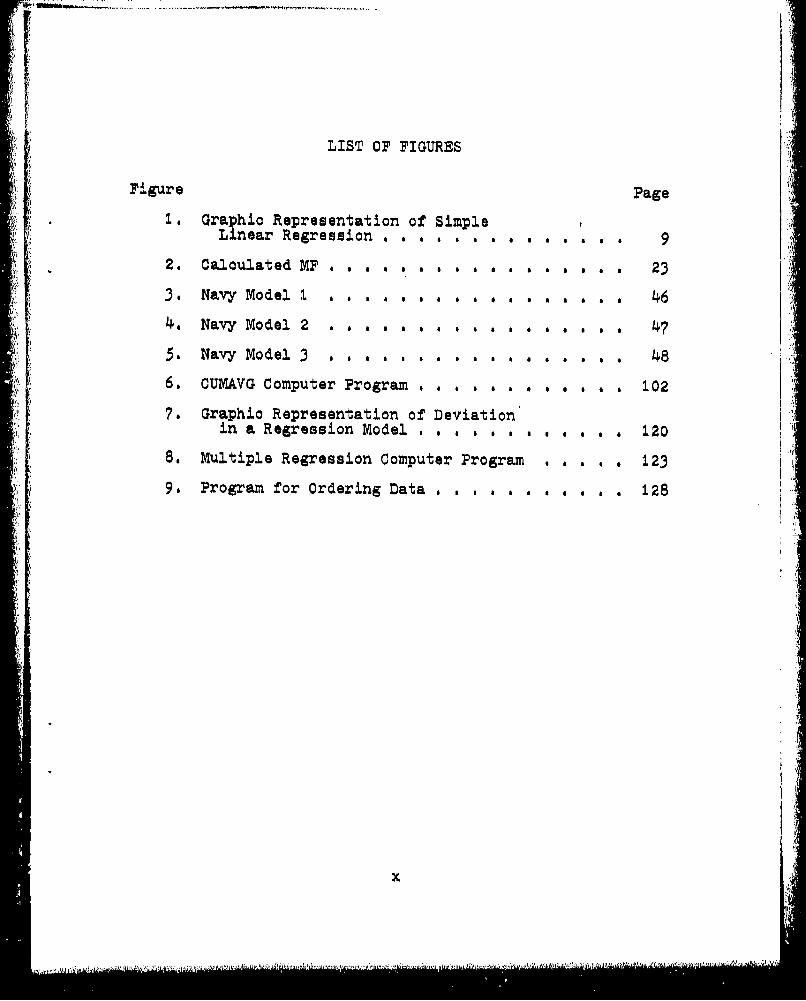
LIST OF FIGURES
Figure Page1. Graphic Representation of Simple
Linear Regression.. . . ... .. . . 9
2. Calculated MFd,,, . .... .... 23
3. Navy Model I . . . . . .o . 46
4. Navy Model 2 47 . * * . * . a . . . . . . . . 7
5. Navy Model 3 . . . . . . . . . . . . . . . . . 48
6. CUMAVG Computer Program a a , a a a a a . a . a 102
7. Graphic Representation of Deviationin a Regression Model, 120
8. Multiple Regression Computer Program . a . . . 123
9. Program for Ordering Data,,., a a a a a . 128
x•HUw
Chapter i
INTRODUCTION
Background
Today's military managers are faced with increasing
systems costs. Because of these increasing costs, managers
must insure that every defense dollar is spent in the most
efficient way possible.
DOD is engaged in an effort to reduce its hardwarecosts. While the military's defense costs are esca-lating, its responsibility to a sustained nationalsecurity persists, It is therefore DOD's desire tore-evaluate existing acquisition procedures and findnew ones in its drive to procure the best hardwarevalue [1811].
One area where this increasing cost is especially true is
in the acquisition of aircraft weapons systems. A driving
factor in the aircraft cost is the turbine engine, and
therefore acquisition managers have been tasked with
developing cost estimating methods that will more accurately
predict engine cost. At present there are several cost
estimation models which can be used in the different phases
of the acquisition process, The primary area of interest in
this study will be cost estimation of turbine engines which
are in the early development stage,
Problem Statemen Ii
The Propulsion Branch, Turbine Engine Division,
Air Force Aero Propulsion Laboratory (AFAPL/TBP) Wright-i1
Patterson AFB, Ohio needs a model which can be used to
estimate the cost of the turbine engine early in its
development stage.
Justification
The Turbine Engine Division is one of four divisions
within the AFAPL. Its mission is the development of
advanced engines for possible use in future weapons systems.
Within the Turbine Engine Division there are four branchess
(1) the Performance Branch, which conducts basic engine
research, (2) the Components Branch, which conducts explor-atory research--working mainly with improvement of engine
components, (3) the Propulsion Branch, which works in
advanced engine development, and (4) the Engine Development
Branch, which matches advanced engines developed in the
Propulsion Branch to a specific mission need. The
Propulsion Branch uses components developed by the
Components Branch to design actual engines. Some of these
engines are built and tested while others remain only
concepts on paper. Although these engines could be used in
future weapons systems, normally they are not. Instead,
when the requirements for a weapon system are identified,
the technology learned in Propulsion Branch engines, and
possibly even components of the engines, are used to develop
an operational engine to be used in the weapon system (17).
The research topic was generated by the Propulsion
Branch of the Turbine Engine Division. Since the possibility
2
does exist that the complete engines or improved components
developed by the Propulsion Branch will be used by some Air
Force agency in the acquisition of a new weapon system, the
Propulsion Branch must be able to accurately predict the
cost of these advanced engines (17).
The accurate estimation of engine costs in the early
development stages is necessary today in view of the
increased emphasis on tighter defense budgets. This
increased interest in cost estimation was illustrated by
the following statement in OMB Circular No. A-109,
Maintain a capability to, Estimate . . . costs forsystem development, engineering, design, demonstration,test, production, operation and support. . . Estimate£ . ,cost during system design concept evaluation . .to ensure appropriate tradeoffs among investment costs,ownership costs, schedules, and performance £615].
If the Air Force is to maintain its combat readiness despite
scarce money resources, then it must be able to accurately
predict the spiraling costs of its new weapon systems.
Since a decrease in these costs is nowhere in sight, the
Air Force must be able to anticipate and plan for the rising
costs in its acquisition of new weapon systems (18:3-6).
One of the major cost driving factors of a weapon
system is the turbine engine, which has not been exempt from
the problem of rising costs. There are many reasons for the
increasing cost of today's engines. Growing inflation is
one, but the increased performance requirements of today's
advanced technology engines have also had a great effect on
cost, Such requirements as improved thrust to weight ratios,
3
I''
improved fuel efficiency, and less noise and air pollution
have been met, but the result has been increasing cost.
For example, to obtain the thrust required in high
technology engines, one of the trade-offs has been a drastic
rise in turbine inlet temperatures. Techniques were
developed to compensate for these higher temperatures. One
such technique was turbine air cooling. Air cooling is
accomplished by forcing air through passageways drilled in
the turbine blade (22t69-73).
Another procedure for coping with the hotter
temperatures has been through the development of exotic
super-alloys. Through the use of these metals, engine
designers have developed blades that con sustain temperatures
up to 21000 F.
The performance results of these turbine sections
have been good, but the cost is high. For example, the
price of an advanced technology turbine disk ranges from
$25,000 to $30,000 (12t81-82), The reasons for the high
prices are the expensive machining techniques and the
increase in cost of metals. According to Aviation Week,
the commodity price of some basic metals used in the
aircraft industry has risen by 125 percent since 1960
(28,73-77). Scientists are looking at ways to reduce these
costs, such as the development of cheaper composite
materials, but it is still apparent that acquisition
managers will be faced with the problem of expensive engines
............ ...... . .... .... ... • •. ,
• ,' ..
I I II II1
in the future. Cost estimation is one tool that could be
used to help manage rising costs.
Several cost estimation models exist; however, only
one of these models was specifically designed for use on the
types of engines of primary interest to the Propulsion
Branch. The results of previous studies have indicated that
some of these models are more accurate than others. When
dealing with expensive engines, however, small errors in
cost estimation models can lead to disastrous results.
For example, one of the models available was
developed by the Rand Corporation. Research was conducted
using this model to estimate the cost of the F100 turbine
engine. The estimated cost of the engine using the Rand
model was $675,359 in fiscal year (FY) 1970 dollars. The
actual FY76 cost of the engine was $2,000,000 which
equates to $1,148,000 in FY70 dollars (18t5). Since
Propulsion Branch analysts desire an estimated value within
25 percent of the actual cost, this underestimation of
$472,641 is unacceptable. Therefore, further research Jis
required to determine which of the existing models are most
appropriate for the needs of the Propulsion Branch (1?).
5
Chapter 2
LITERATURE REVIEW
Cost Estimation
Estimating is the process of reckoning in dollarsthe sum necessary to manufacture a product at somefuture time by calculating and projecting the futurecosts of men, materials, methods, and management. Itis a tart of every business. The production of anyitem as tied to estimating from the time it isconsidored feasible, through development and engineering,until the cost of every nut, bolt, and screw can bepriced as a part of the total cost for the job [8si].
military service manuals on cost estimation listed as many
as five different methods, other sources listed many other
variations such as synthesis, analysis, roundtable
estimating, estimating by comparison, detailed estimating,
analytical appraisal, comparative analysis, and statistical
analysis (2t2), These methods can be placed in two
categories--engineering-accounting and statistical (1j2).
Enxineering-accounting. The engineering accounting
approach, also referred to as the industrial engineering
approach, the grass roots approach, the building block
approach, or the bottom up approach,
entails the examination of separate items ofwork at a low level of the work break down structurewith detailed estimates developed for the functionalcosts of engineering, manufacturing, quality control,etc, In turn, these are broken down by labor material,and other elements of cost for each item [ 1:3j.
6VA
The summation of these individual costs is used to compute
the total system cost (17), According to a Rand report,
Engineering estimating procedures requireconsiderably more personnel and data than arelikely to be available to government agenciesunder any foreseable conditions C2o5].
Nevertheless, the engineering method is sometimes used in
the later phases of the acquisition process when more
detailed information is known. One advantage of the
engineering method is increased accuracy because of the
detail required in arriving at the final cost, However, it
is also the most expensive and time consuming, Many people
are required to analyze a system's components and determine
the price of each (2s2-8). Since the engineering accounting
approach entails more resources than the statistical method,
the latter is the most widely used in cost estimation,
Statistical analysis. The use of statistical
analysis in cost estimation has proven to be one of the
more practical methods. The key to this methodology is the
extensive use of historical data pertinent to the system
being studied. Pertinent historical data may be defined
as characteristics of previous systems which are similar to
characteristics of the system under consideration (2113-16).
Statistical methods are used to analyze data and establish
cost driving relationships between the old and new system
(15 1i-2). For example, it might be determined from
analyzing historical data in the automobile manufacturing
7
............ .......... .. ... ..... ...
industry that when the speed capability of a new model
automobile increased by a certain amount, the price also
increased by a proportional amount. By using the rela-
tionship of speed to price, general equations can be
developed to estimate the price of any new car. This
simplified example demonstrates one of the basic concepts
used in statistical cost estimation--linear regression
(29,315-326).
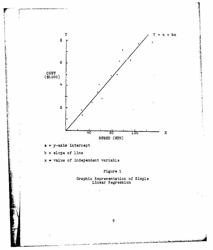
Linear regression. Linear regression is a method
commonly used in cost estimation to analyze historical data,
One characteristic of the system, for example the speed of
a car versus cost, is chosen, and all the data collected
concerning cost versus speed are plotted on a two dimen-
sional graph. The independent variable speed is plotted on
the horizontal axis (x) against the dependent variable cost
on the vertical axis (y). Once the speed/cost data are
plotted, a line is fitted through the plotted data points.
By determining the slope of the line, the x-axis intercept,
and the y-axis intercept, a linear equation describing this
line can be formulated. This general equation can then be
used to estimate the price of any car based on the desired
speed capability of the car (Figure 1). Detailed procedures
for fitting a line can be found in basic statistics texts
(30,368-395).
A problem that must be considered when using
regression analysis is the significance of the derived
8
Y Y a~bx
S *1C OST
($1000)
.il 4I
2 - I
0 00 X
SPEED (MPH)
a = y-axis intercept
b = slope of line
x = value of independent variable
Figure 1
Graphic Representation of SimpleLinear Regression
V1
9
equation. One method of testing for a significant rela-
tionship between x and y is called the t-ratio or ratio of
a coefficient to its standard error. The procedure develops
a hypothesis that x and y are not related, and then testing
of the data is performed to determine if the null hypothesis
can be rejected (29,341-347). (See Appendix D for further
explanation of regression analysis.)
Turbine Engine Cost
Estimation
The statistical methods previously discussed were
the primary methods used in developing turbine engine cost
estimation models for Air Force use (2,v). When developing
an engine cost estimating model using linear regression
techniques, engine parameters must be selected which will
have an effect on production cost. This relationship,
between cost and parameters, is called a Cost Estimating
Relationship (CER), and the method is termed Parametric
i Costing (2179-87). For turbine engines these CERs include
such parameters as thrust, weight, maximum RPM, turbine inlet
j temperature, cruise mach, and specific fuel consumption
(20v). Historical data concerning engine parameters are
collected, and linear regression is used to determine which
parameters chow the greatest relationship to production cost.
In the regression model, the engine parameters are the
independent variables and production cost is the dependent
variable. From the regression analysis, generalized
10
Ilk... ! ,•.•,• • /.r,.•!:!• • ;• ••• •'''
equations are developed which can be used to estimate the
cost of the engine (2033-50).
Rand model. The Rand Corporation has conductedextensive research in the cost estimation area. Themajority of its work deals with parametric costing
techniques. Rand's latest effort using parametric costing
was an analysis of turbine engine life cycle costs. Of
particular interest to this research effort was the portion
of the Rand study dealing with engine production cost
estimation.
As with most other cost estimation models, the Rand
model used several CERs in its equations. Rand studied
many different engine parameters and determined that
parameters such as thrust, weight, turbine inlet temperature,
and specific fuel consumption were the primary cost drivers
in engine production cost (i9 1 i3). However, at this point,
Rand varied from the standard technique of showing a direct
relationship between an engine parameter, such as thrust,
and cost. Instead, Rand introduced a level of technology
factor in its model. Rand believed that if an engine pushes
the state-of-the-art, the result would be an increase in
cost, and this factor should be part of the cost estimating
equation (19,13).
In using the state-of-the-art factor in the model,
"Rand introduced two terms which are not used in other cost
ii
estimating models. These terms are time of arrival (TOA)
and model qualification test (MQT). TOA is the time
designated that an engine passes D/T, and is ready for full
production (20o5). Rand defined XT as
. the final military qualification, normally150 hours, after which the engine is considered to besufficiently developed for installation in a productionaircraft C27,8].
Rand used a separate regression model containing the
previously described engine parameters to calculate TOA.
This TOA was given in quarters of a year with October 1942
used as the base year. The calculated TOA was compared to
the engine actual TOA, and the difference of the two was the
engine's delta TOA (ATOA). The ATOA is the state-of-the-art
factor which is used in the CER to calculate the estimated
production cost.For example, assume that a new engine is being
developed, and the values required for the cost estimation
model are known. The calculated TOA is determined from the
computation of the known values in the equation. If this
TOA is higher than the engine's actual TOA, the state-of-the-
art required to build this engine is being pushed, and the
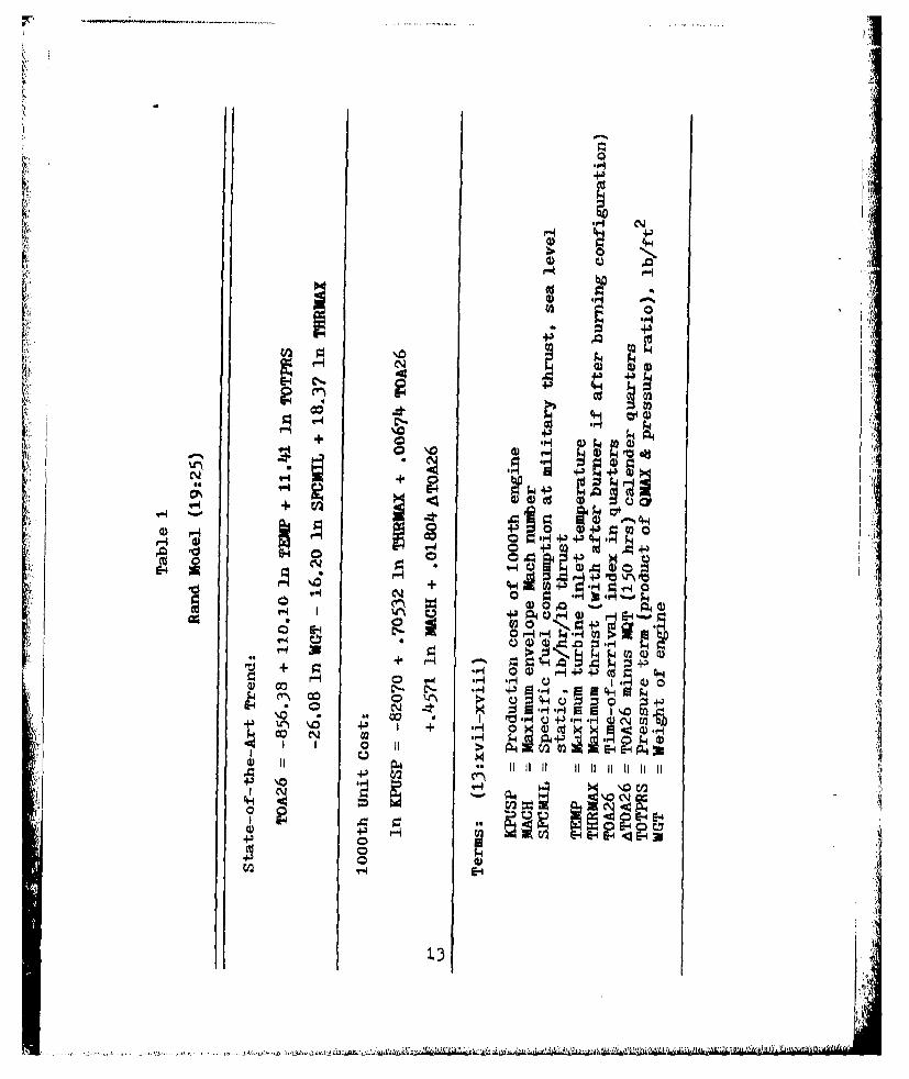
result will be increased cost. Table I is a listing of the
equations for the Rand model (2013-19).
Rand's first report on this type of cost estimation
model was in 1974. A research effort conducted by Captains
Rodney J. Mullineaux and Michael A. Yanke reported the
results of the model using data they had collected on the
12
4 4J.) 4-1
-4-1
,,- P4 (t )
a +,
0)0
0 0 -P 4J 0q C
1-4 0 1-l C
N 0 0. -' % m~X%Z .4 co 04) ( f
+. 9 0) ft)co 0 (*3')
0) ~ '- C' .~ ~I 4H00
4-2
* * *HH~~13
------- ............... .. .~ .. .H . ~ .... ...
F100 engine. As indicated earlier, the estimated cost of
this engine using the Rand model was $472,641 below the
actual engine cost--an error of 70% (1805).
In 1977 Rand issued another report in which the data
base used to construct the original cost estimation model
had been updated, thus leading to improvements in the model.
The model shown in Table I is based on this 1977 report.
Currently, no formal study of the new model has been
conducted, although a cost analyst who has been working with
this model indicated that the estimated costs are agzin
below the actual engine costs.
Although the Rand model could be used by the
Propulsion Branch, the model design makes it more appro-
priate for use in earlier development stages where less
detail about an engine is known (17).
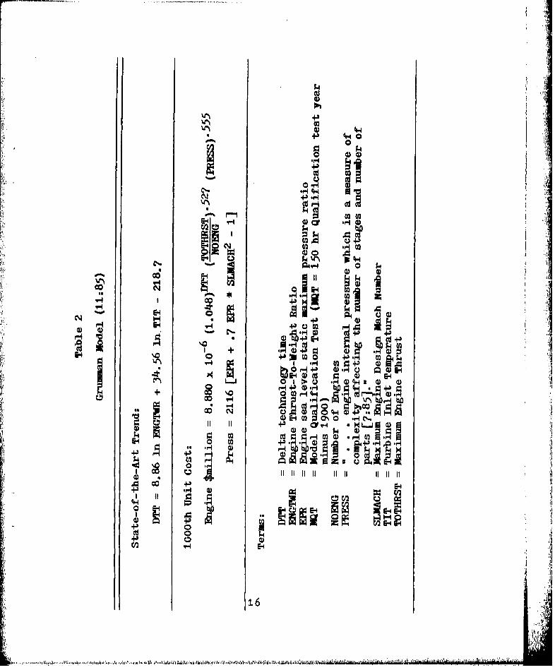
Grumman model. The Grumman model is another cost
estimation model which was based on the Rand concept just
discussed. The Grumman engine production cost model was
part of a Life Cycle Cost Model developed by the Grumman
Aerospace Corporation for the Air Force Flight Dynamics
Laboratory at Wright-Patterson APB, Ohio. It was designed
to predict the total cost of an advanced aircraft systemV including research, development, testing, and engineering,
production, initial supportl and operations and support
costs. A portion of the model deals specifically with the
prediction of engine costs (11ii)
_i
As in the Rand model, the Grumman model relates cost
to design parameters and vehicle performance requirements.
Grumman's data base was developed using Rand's cost
estimation data base and industry sources. The cost data
from these sources were combined with the appropriate engine
design parameters and regressed to produce CERs, as explained
earlier (11J19). This model also relates the production
costs to advances in engine technology, Therefore, as in
the Rand model, a TOA exists in the Grumman model, but
instead of TOA Grumman used the term Delta Technology Time
(DTT) (1t,66),
This model was designed to be used with a complete
weapon system; thus, the Propulsion Laboratory and other
departments within AAPL have not used this model and are
not aware of its value or credibility at this time. At
present, the model is being tested on new engines to
evaluate its practicability in cost estimation of advanced
engines (17). (See Table 2 for the Grumman Model.)
Mullineaux and Yanke model. In June 1976 Captains
Mullineaux and Yanke of the Air Force Institute of
Technology, Wright-Patterson APB, Ohio, conducted a study
to build a model for AFAPL for estimating engine costs.
This study led to the development of a new model, Model 8
in their thesis. This methodology was built upon the CERs
developed by Rand with a few modifications--the addition of
material factors developed by the Navy, to be discussed15
S. .. . .. . - " .-_ . ...... • " .:------. .. ... . , . . .... . -. .. .. : l "
4J i
Cd
VI C Ci
- $0
--0 rq C(D
E-11
4J (0 4 4
v4
41 0yV4 0 ~
r1.6
4J;'
later in the Maurer Factor (MF) approach. Mullineaux and
Yanks felt that the inclusion of a material factor within
their model " . . . would automatically update the cost-
estimating model as changes in technology occurred CI8,21J."
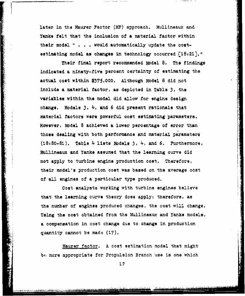
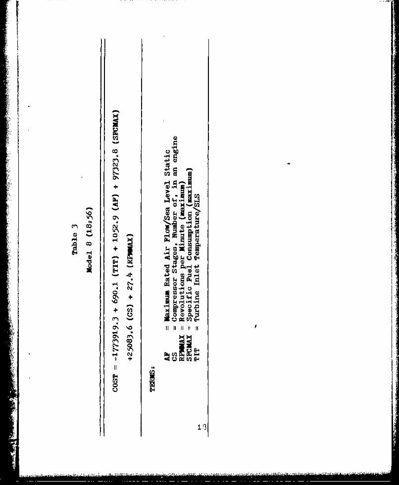
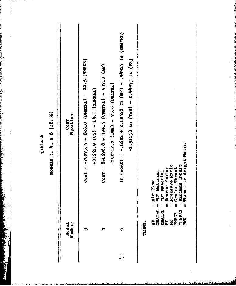
Their final report recommended Model 8. The findings
indicated a ninety-five percent certainty of estimating the
actual cost within $375,000. Although Model 8 did not
include a material factor, as depicted in Table 3, the
variables within the model did allow for engine design
change. Models 3, 4, and 6 did present rationale that
material factors were powerful cost estimating parameters.
However, Model 8 achieved a lower percentage of error than
those dealing with both performance and material parameters
(I8,80-81). Table 4 lists Models 3, 4, and 6. Furthermore,
IlMullineaux and Yanks assumed that the learning curve did
not apply to turbine engine production cost. Therefore,
their model's production cost was based on the average cost
of all engines of a particular type produced.
Cost analysts working with turbine engines believe
that the learning curve theory does apply, therefore, as
the number of engines produced changes, the cost will change.
Using the cost obtained from the Mullineaux and Yanks models,
a compensation in cost change due to change in production
quantity cannot be made (17).
Maurer factor. A cost estimation model that might
bf, more appropriate for Propulsion Branch use is one which
.......... I.I
N V2
444
-*4 6V~2 0)o
0
"4$
S0 0 )
4.)
C',-W
000% N~
4J4 -H 0%oo mf 40
co~I rnC.Jr.-o
+ CO 4-
1 4-3
'A~~ 4- " '
incorporates the Maurer Factor CER. The MP, developed by
the late Mr. Richard J. Maurer, was a parameter used in the
Navy cost estimation models. The basic concept behind the
MF method was that the cost of a turbine engine is related
to the materials required to build the engine (3,2-5).
In the mid 1960s the Navy began extensive research
into the "why and how" of engine costs. As higher
technology engines became a reality, the Navy realized that
its costing methods were not adequate. After surveying
existing costing methodologies and CERs, the Navy decided
that the engine parameters used in its cost estimation
models were not valid. Instead, the Navy developed the
basic rationale that the cost of an engine, in great part
if not entirely, is governed by the type of material as well
as the weight of the raw material employed in the manufacture
of an engine (3,2-5).
This rationale assumes that most of the physicaland thermodynamic technology areas associated withengine-compressor stage loading, maximum turbinetemperatures, specific weights, etc.--are closelyinterrelated with the metallurgical technologies.This assumption is probably more true of the aircraftindustry than any other aerospace industry because ofthe severe stress and temperature environmentexperienced by a Jet engine C3t2-51.
As a result of this concept of the relationship of
materials to cost, the Navy began initial efforts in defining
a material parameter to describe engine costs. Mr. Richard
Maurer did extensive work in classifying all the materials
used in a Jet engine into seven material categories, and
20
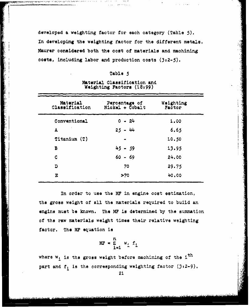
developed a weighting factor for each category (Table 5).
In developing the weighting factor for the different metals,
Maurer considered both the cost of materials and machining
costs, including labor and production costs (3s2-5).
Table 5
Material Classification andWeighting Factors (18s99)
Material Percentage of WeightingClassification Nickel + Cobalt Factor
Conventional 0 - 24 1.000
A 25 -44 6.65
Titanium (T) - 10.50
B 45 -59 13-95
C 60 - 69 24.00
D 70 29.75
2 >"70 40,00
In order to use the M. in engine cost estimation,
the gross weight of all the materials required to build an
engine must be known. The MF is determined by the summation
of the raw materials weight times their relative weighting
factor. The MF equation is
nMP. = wi fi
ial
where wi is the gross weight before machining of the ith
part and fi is the corresponding weighting factor (3,2-9).
21.
.• , .. . ... .. ..
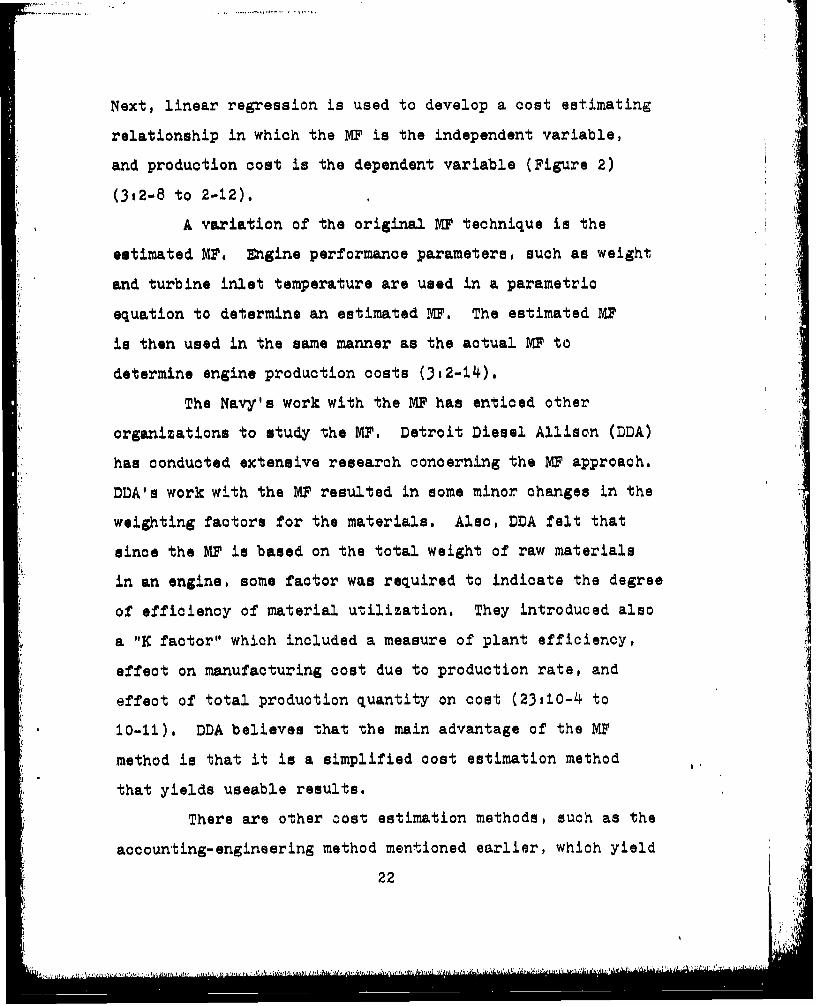
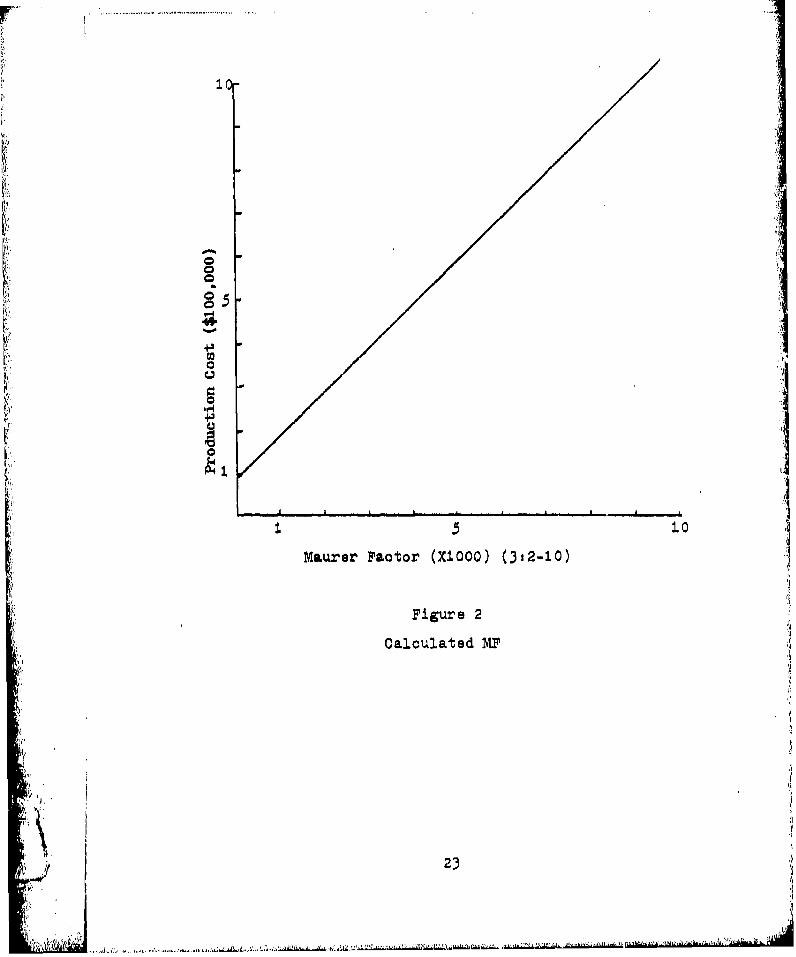
Next, linear regression is used to develop a cost estimating
relationship in which the MF is the independent variable,
and production cost is the dependent variable (Figure 2)
(3,2-8 to 2-12).
A variation of the original MF technique is the
estimated MF. Engine performance parameters, such as weight
and turbine inlet temperature are used in a parametric
equation to determine an estimated .IF, The estimated Ml
is then used in the same manner as the actual MP to
determine engine production costs (3t2-14).
The Navy's work with the MP has enticed other
organizations to study the MP. Detroit Diesel Allison (DDA)
has conducted extensive research concerning the MY approach.
DDA's work with the Ml resulted in some minor changes in the
weighting factors for the materials. Also, DDA felt that
since the Ml is based on the total weight of raw materials
in an engine, some factor was required to indicate the degree
of efficiency of material utilization. They introduced also
a "K factor" which included a measure of plant efficiency,
effect on manufacturing cost due to production rate, and
effect of total production quantity on cost (23si0-4 to
* 10-11), DDA believes that the main advantage of the Ml
method is that it is a simplified cost estimation method
that yields useable results.
There are other cost estimation methods, such as the
accounting-engineering method mentioned earlier, which yield
22'i
005-
*11
50
I . IIi
Maurer Pactor (XiOOO) (3,2-10)
Figure 2
Calculated MF
;/ 234 1.
j
better results but also require many more man-hours and
much more detailed information about the engine. Ordinarily
this information would not be available in the early stage
of engine development (23,10-18),
The Learning Curve
Another aspect that should be taken into account in
cost estimation models is the learning curve. The basic
theory is that when a new task is undertaken by an individual
or group, continuous repetition of that task will tend to
improve efficiency (4,3). The learning process prevails in
many industries; its existence has been verified by
empirical data and controlled tests. A Rand report stated
that
the basis of learning-curve theory is thateach time the total quantity of items produced doubles,the cost per item is reduced to a constant percentageof its previous cost C2193].
For example, in a manufacturing process possessing
an 80% learning curve, the cost of producing the 2nd unit
would be 80% of the cost of producing the Ist unit, and the
cost of producing the 32nd unit would be 80% of the cost of
producing the 16th unit (17). The learning curve seems to
fit most appropriately in situations where there is: (1) a
high proportion of manual labor, (2) uninterrupted
production, (3) production of complex items, (4) no major
technological changes, (5) continuous pressure to improve,
or (6) no external rate changes (16). Although there are
24
many factors contributing to the learning curve theory,
4 the most commonly mentioned are,
1. Job familiarization by workmen.
2. General improvement in plant coordination and
organization.
3. Development of more efficient operations.
4. Substitution of casts or forged components for
machined components.
5, Improvements in overall management (2t94).
Rand also believed that a learning curve exists for
unit materials cost, Worlknen learn to work more efficiently
with the raw materials, and management learns to order
4, materials in shapes and sizes which are more appropriate for
the job, thereby reducing the waste involved in fabrication,
The result is a reduction in overall material cost as the
learning process continues (2195-96).
Since the MY is based on the relationship of
materials to production cost, this research effort will
investigate the application of the learning curve to the
MF, (See Appendix B for explanation of the learning curve.)
9bJectives
The objective of this research study was to determine
if the Maurer Factor cost estimation method could be used
by the Propulsion Branch of the Air Force Aero Propulsion
Laboratory. The study will include an examination of the
procedures required to use the MF cost estimation method.
25
• ' 2 .... . 2 _ ".. . .
The accuracy of the results obtained from the MF
technique and the amount of time and effort required to usethe technique will determine the value of the technique to
the Propulsion Branch.
The research effort will also investigate the
possible application of the learning curve theory to turbineengine cost.
Research Questions
1. What steps are necessary to develop and use the
Maurer Factor cost estimation model?
2. What results can be achieved concerning turbine
engine cost estimation in the early development stage by
using the Maurer Factor cost estimation model?
3. Is the learning curve applicable in turbine
engine cost estimation?
4, How can the learning curve be incorporated with
the Maurer Factor technique?
Research Hy-pothesis
A model based.on engine performance parameters
can be developed which will estimate the Maurer Factor.
Summary
Increasing costs in aircraft weapons systems have
been evidenced by the acquisition managers, In an attempt
to use limited funds more efficiently, cost analysts require 2
cost estimation techniques which will accurately predict
26
• - -• -• ' ' - •- • •- • -"" -- '• - I
future costs. The Propulsion Branch analysts are familiar
with four estimation teohniques--(1) the Rand model, (2) the
Grumman model, (3) the Mullineaux and Yanks model, and (4)
the Maurer Factor model. However, they have specifically
requested the study of the MP for use in their work with
turbine engines. The MF is a statistical and not an
industrial-engineering approach of achieving a cost
estimate. This research will analyze the MP's usefulness
in predicting turbine engine production costs in the early
development stage.
27
i...............
Chapter 3
RESEARCH METHODOLOGY
Overview
The research methodology was designed to determine
the estimated cost of turbine engines using the Maurer
Factor (MP) technique. Additionally, a model was developed
which will estimate the MF. In this model, estimated
Maurer Factor (EMF) was the dependent variable and engine
performance parameters and engine categories were the .1independent variables. 4
Variables of Interest
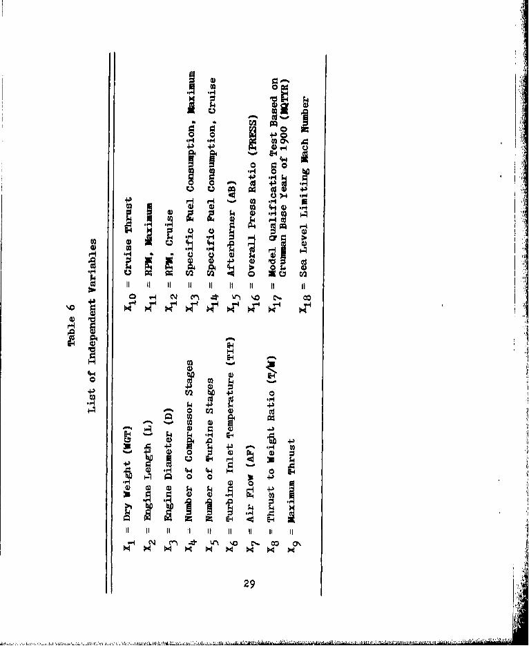
The variables of interest included turbine engine
materials, engine performance parameters, and engine
classification based on afterburner versus non-afterburner,
The materials variable represented the summation of all
materials in a turbine engine. RPM, turbine inlet
temperature, and thrust were the performance parameters
used in developing the EMF model (Table 6).
Justification of Variable--Selection
As discussed earlier, several studies indicated that
engine materials were an important cost-driving factor
28
.4J)
04
4)A0)
E-4
4-2
0 W 0'~ w
ca~
0 .H ~ C4.4-)
~~4. CH o . C-~
~~'4 E'4- 4
29
". j� m .. f .! V -t •. .... ...... .....
(31 151 181 23). For this study the MF was used as the
material factor in the cost estimation model.
The variables listed in Table 6 were used to
develop the EKF model. These variables were determined
through discussion with the Propulsion Branch cost analysts
and through information gained from research studies
conducted by the Navy and the Rand Corporation (81 171 201
27). Several combinations of these independent variables
were used in developing the model.
Selection of Independent
Variables
Three basic requirements were considered in
selecting variables for the cost estimation model,
1. The variable (MF) had to exhibit a logicalrelationship as a cost-driving factor (29,37L-376).
2. The variables in the EMP model had to show a
logical relationship to IF.
3. The model is proposed for use by the Propulsion
Branchl therefore, independent variables were selected which
could be supported by data available to the cost analyst
in the early development stage of an engine.
Method of Data Collection
Two methods were used to obtain data, First, the
data base created by Captains Mullineaux and Yanke was used.
The data base contains engine performance parameters for 93
30
.,~, .') ~ 1 t, ..r~ t , ,. i t fj A I . ... ................... . .. .' . .
turbine engines, However, the gross weight of individual
components in some of the engines was not available;
therefore, theme engines could not be used for M?•
calculations.
Another major source of data was the USAF Propulsion
Characteristics Summary (Airbreathing), This document is
commonly referred to as the Gray Book. Data in the Gray
Book concerning engine production lots and engine prices
were used for investigating learning curve characteristics
in turbine engine production. Also, the data collection
plan included the use of the Navy's equivalent to the Gray
Book,
The DD Form 346, Abbreviated Summary Bill of
Materials, was another data source. The 346 gives a break-
down of an engine by components and lists the gross weight
of these components, before machining, along with the type
of material of each component, The 346 is supplied to the
Air Force by the contractor, and the data contained in it
are vital to performing MF computations. An example of the
data found on the DD Form 346 is shown in Table 7.
The final source of data was material type and
gross weight of engine components as supplied by engine
manufacturers. A complete set of this type of data was
obtained from the manufacturer of one of the validation
engines (Appendix C).
31
uiww ý1 a
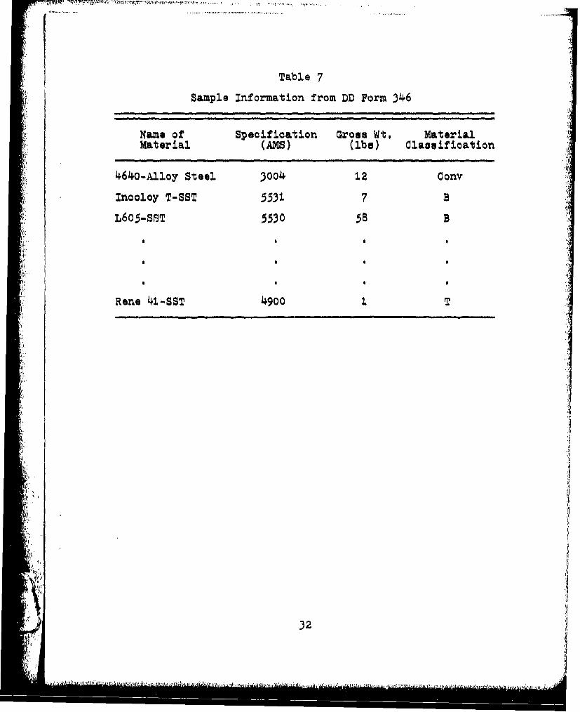
Table 7
Sample Information from DD Form 346
Name of Specification Gross Wt. MaterialMaterial (AMS) (lbs) Claggification
4640-Alloy Steel 3004 12 Conv
Inooloy T-SST 5531 7 B
L605-SST 5530 58 B
Rene 41-SST 49OO I T
32
=OioI-- • ,*.' '
310
Before the data obtained from the DD Form 346 and
from individual contractors could be used for MP compu-
tations, the different materials for all of the engine
components were classified and assigned to one of the seven
categories shown in Table 5. The classification involved
several steps.
First, the different alloys were assigned an
Aerospace Material Specification (AMS) number (13,1-31).
Each AMS number was assigned to one of the seven MP'
categories shown in Table 5. The AMS conversion tables
used by Capts Mullineaux and Yanks were used to categorize
the AMS numbers by MP category (18,101-103). An example of
this table is shown in Table 8. A complete explanation of
the materials classification process is in Appendix C,
Po~ulation and Sammle
Description
The population consisted of all turbine engines
which have been used in United States military aircraft and
advanced engines currently under development for possible
use in future weapon systems.
The research conducted for the literature review
indicated that data pertinent to the calculation of the ME
may be difficult to obtain. Therefore, a sample of
opportunity was used in our data collection effort.
33
............
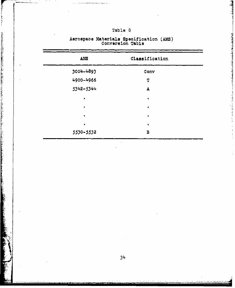
Table 8
Aerospaoe Materials Speoification (AMS)Conversion Table
AMS Classifioation
3004-4893 Cono4900-4966T
5342-5344 A
* 0
5530-5532 B
34
Model Justification
The objectives of the study included an investigation
of the MF process and the development of an estimated MF
model. The MF cost estimation concept was chosen because:
I, A model is needed which is not complicated and
obtains reasonable results, Engineers and cost analysts
working in the turbine engine field consider an estimate
within 25 percent of the actual cost to be reasonable (17).
2. Engine cost appears to be highly related to
materials; therefore, the model should be sensitive to
materials (3'2-5).
3. The higher the engineering technology in an
engine the higher the cost; therefore, the model must be
sensitive to technology changes (13,81-8.2). Technology is
compensated for in the MP model through the weighting
factors assigned to the seven MF materials classifications
(3t2-5).
The development of 'the EMF model was studied because
the material data required to compute the actual MX may not
be readily available to cost analysts in the Propulsion
Branch. Since the literature review indicated that the use
of a material factor in the turbine engine cost estimation
model is appropriate, a relationship between engine
parameters and MlF was used to develop the EWi model. The
Navy's successful use of the MF technique verifies the
importance of the material factor in estimating engine
cost (7),35
............................... ,, ,
Model Development
One part of this research effort was directed toward
developing a model that could be used to estimate the MY.
The MV can then be used in the MF cost estimation models
developed by the Navy. To develop the TMU model, it was
necessary to establish and verify appropriate relationships
between engine parameters and MP.
After the appropriate variables were identified,
such as the relationship of engine air flow and MPI engine
thrust and MFj and turbine inlet temperature and MP, some
meaningful way had to be used to combine these variables
into a useable model. Regression analysis was used to
analyze and combine the variables into a model which
resulted in an EMF model.
Rearession Analysis
Multiple regression was used to develop the EMF
model, Multiple regression is an extension of the simple
linear regression technique discussed in Chapter 2.
However, in multiple regression a number of independent
variables may be used, The advantage of this method is
that the effects of several independent variables on the
dependent variable may be determined, Also as independent
variables are added to the model, the amount of unexplained
variation in the model is reduced (29,359-362).
The independent variables were the engine performance
parameters as listed in Table 6, The dependent variable was36 •
MF. An explanation of the multiple regression technique
used to develop the Me model is given in Appendix D.
Validation Process
The Maurer Factor technigue. Before EMP model
validation could be accomplished, the cost estimating
relationship of calculated MP to cost had to be validated,
The calculated MF for five engines was used in three MF
models developed by the Navy. Hereafter, these engines
will be referred to as validatioa engines i, 6, 7, 8, and 9.
Engine I is an advanced technology engine, and engines 6,
7,8, and 9 are turbojet engines currently in use, The
estimated costs of the validation engines were compared to
their actual costs. Engines 1, 6, 7, 8, and 9 were selected
as the validation engines because the data requiied to
compute the MlF for these engines were available, and their
actual costs could be determined. Therefore, a meaningful
comparison between actual engine cost and the estimated
cost could be made. After the Navy MF models had been
validated, the EMF model validation could be accomplished.
Estimated Maurer Factor model validation. The EM?
models were developed using data from the Mulltneaux and
Yanke data base, Five advanced technology engines were
used to validate the EMF models; hereafter referred to as
engines 1, 2, 3, 4, and 5,
37- Ct
Certain performance parameters for engines 1, 2, 3r
4, and 5 were used in the ENF models to arrive at an EMP. ,
The computed EMF was then used in the three Navy MD models.
The resultant estimated costs were compared to the actual
cost of engines 1, 2, 3, 4, and 5.
In order to obtain a realistic validation of the EMF
models, engines 1, 2, 3, 4, and 5 were not used as data
points in developing the EMW models.
Selected test criterion. The statistical signif-
icance of the model was determined using F-test and t-tests
with the level of significance set at a = .05. (See
Appendix D for further explanation of these tests.)
Summary List of
Limitatiens
1. The gross weights of some of the engine
components used in calculating the Maurer Factor were
estimates. The estimates were made by the engine manu-
facturers and were assumed to be accurate (17).
2. The independent variable list identified may
not be all-inclusive (17).
Summary List of
T Assumptions
I. Concerning the independent variabless
a. The regression models developed by the Navy
were assumed to represent an accurate regression of turbine
engine cost on Maurer Factor (3,2-13),
38
' I '~ .,,.I!'*',
b. The engine performance parameters used in
developing the EMF regression models were assumed to be the
most representative of the entire set of possible performance
parameters, and i
c, The independent variables met the necessary
criteria for regression analysis. A list of these criteria
can be found in Appendix D.
2. Historical data of past jet engines could be
used to predict the costs of future Jet engines.
39 .
01-
Chapter 4
DATA ANALYSIS AND FINDINGS
Introduction
In this chapter a detailed analysis of the Maurer
Factor (MF) technique and the estimated Maurer Factor (EMP)
models are presented, The results of the estimated costs
of the validation engines obtained using the MF technique
are discussed in an attempt to determine its validity.
Also, a statistical analysis of the EMF models is presented.
The EMF models are discussed in terms of the statistical
findings for each model and the results of the validation
process using the validation engines. The chapter is
summarized by addressing the research questions and the
research hypothesis.
Malirer Factor Cost EstimatingTechnique
Learning curve cost adjustment. The learning curve '3
theory was used to adjust the cost of the validation engines
to the cumulative average cost of 1500 engines. Theadjustment was required because the Navy MF cost estimation
models were based on the cumulative average manufacturing
-ost of 1500 engines, and the costs of the validation
engines were all based on costs other than the cumulative4o ;
average cost of 1500 engines. To make a valid comparison
of the actual cost to the estimated cost, the actual cost
and the estimated cost had to have the same cumulative
average cost basis.
Since validation engines 6, 7, 8, and 9 were engines
in the inventory, historical cost data for these engines
were available. The percent of learning for these engines
was calculated using the computations shown in Appendix B.
After the percent of learning was computed, the cumulative
average cost of engines 6, 7, 8, and 9 was calculated. A
summary of the calculations is presented in Table 9,
Because validation engines ., 2, 3, 4, and 5 were
proposed advanced technology engines, no historical data
were available to calculate the percent of learning. The
learning figures supplied by the manufacturers were used to
adjust the costs of validation engines 1, 2, 3, 4, and 5 to
cumulative average costs (Appendix B). A summary of these
computations is shown in Table 9.
Profit and General and Administrative cost
adustments. In addition to the learning curve cost
adjustment to the validation engines, the engine costs
were adjusted for profit and general and administrative
(G&A) costs. This adjustment was necessary because the
Navy cost models gave an estimated cumulative average
manufacturing cost, but the dollar amounts of the validation
engines were total selling price to DOD. The manufacturing
.41
III i .~
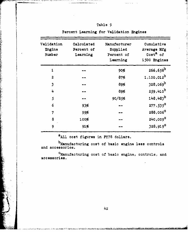
Table 9
Percent Learning for Validation Engines
Validation Calculated Manufacturer CumulativeEngine Percent of Supplied Average MfgNumber Learning Percent of Coslt of
Learning 1500 Engines
I -- 90% 2 6 6 , 6 5 8b
2 -- 87% 100012
3 -- 89% 3 2 8 ,0 6 9b
4-- 89% 25 9,• 1 0b
5 -- 90/85% 1 4 8 , 4 8 3b
6 93% - 27 7 , 535 0c
7 99% -- 288,0060
"8 100% -- 24o,0090
9 91% 328,9190
a All cost figures in PY78 dollars.
bManufacturing cost of basic engine less controls
"and accessorios,
CManufaoturing cost of basic engine, controls, and
accessories.
42
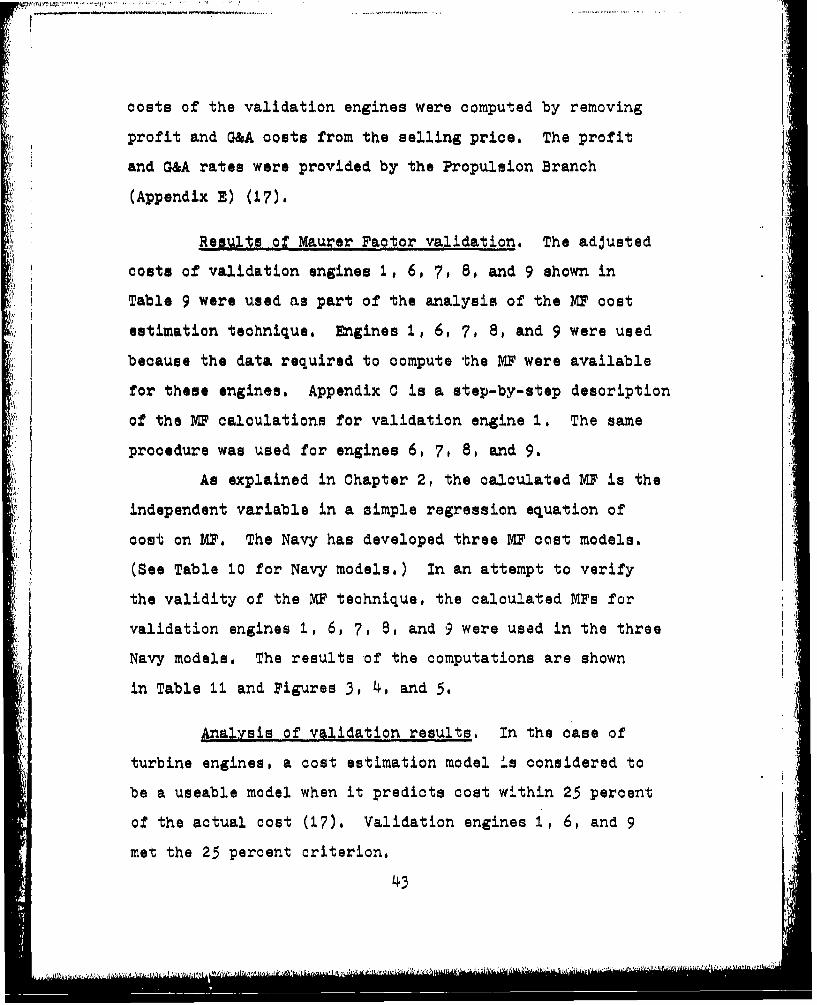
costs of the validation engines were computed by removing
profit and G&A costs from the selling price. The profit
and G&A rates were provided by the Propulsion Branch
(Appendix E) (17).
Results of Maurer Factor validation. The adjusted
costs of validation engines 1, 6, 7, 8, and 9 shown in
Table 9 were used as part of the analysis of the MI cost
estimation technique. Engines 1, 6, 7, 8, and 9 were used
because the data required to compute the MF were available
for these engines. Appendix C is a step-by-step description
of the XF calculations for validation engine 1. The same
procedure was used for engines 6, 7, 8, and 9.
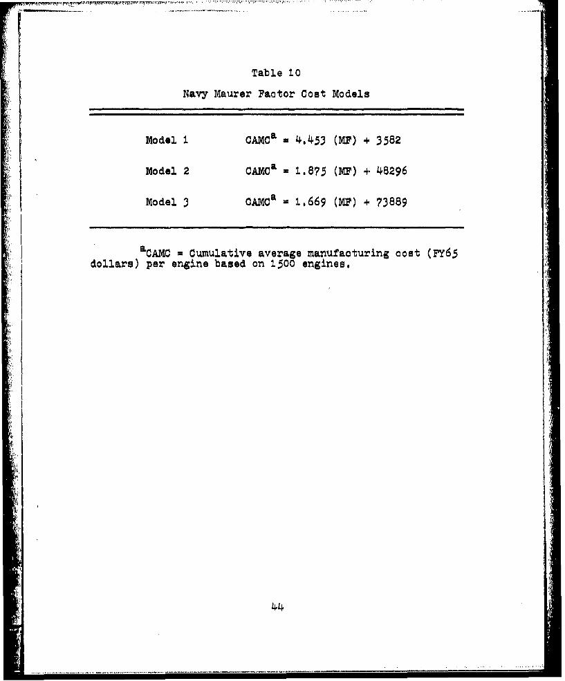
As explained in Chapter 2, the calculated MP is the
independent variable in a simple regression equation of
cost on 10. The Navy has developed three MF cost models.
(See Table 10 for Navy models.) In an attempt to verify
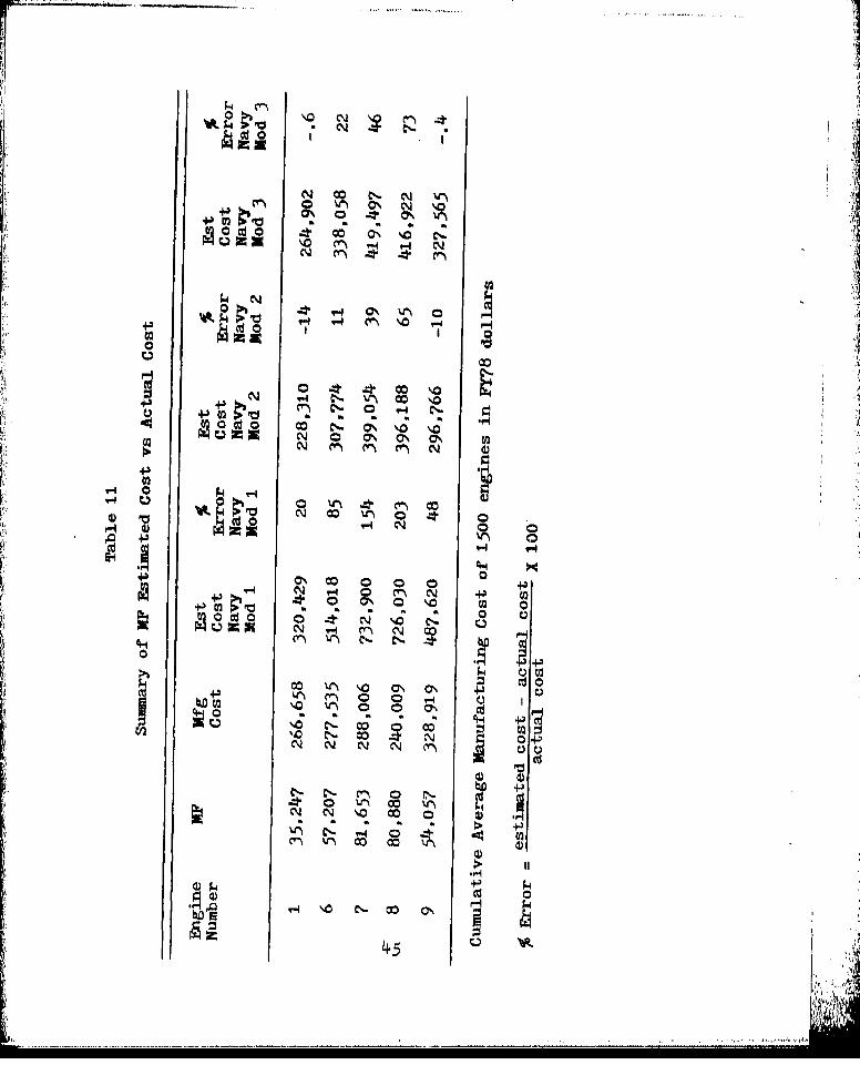
the validity of the MF technique, the calculated MFs for
validation engines 1, 6, 7, 8, and 9 were used in the three
Navy models. The results of the computations are shown
in Table 11 and Figures 3, 4, and 5.
Analysis of validation results. In the case of
turbine engines, a cost estimation model is considered to
be a useable model when it predicts cost within 25 percent
of the actual cost (17). Validation engines 1, 6, and 9
met the 25 percent criterion.
43
. . . . . .......
F£
Table 10
Navy Maurer Factor Cost Models
Model i CAMCa = 4453 (MlF) + 3582
Model 2 CAMCa = 1.875 (Ml') + 48296
Model 3 CAMCa = 1,669 (Ml) + 73889
aCAMC = Cumulative average manufacturing cost (FY65dollars) per engine based on 1500 engines.
44
41*
m \0
02oc
0 c
4JN cc% % 0'V. No cz C'0'ý N
CoN
0t
~4 0 00N CN P C44
0 -0
Co 0 rN % CYN
N co ~N
002
-q 00C 0
45)
L . .........
i ~1.
1,000.
Ji
A A !!
St
4J 5 0 0 -,!:
4-)
oo10 0
100 500 1,000
Actual Cost($1,o000)
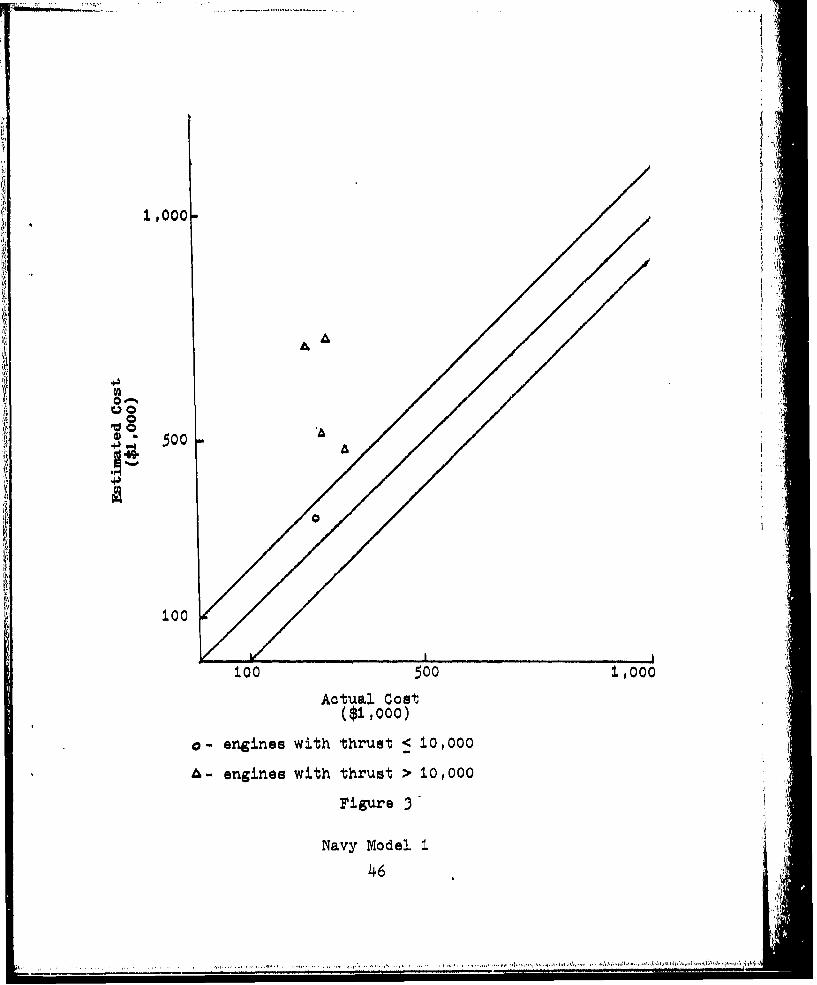
a- engines with thrust < 10,000
A- engines with thrust > 10,0000
Figure 3
Navy Model 1
46
' I I I'I
Il,
1,000 0 4'
+3
4J 50
r A
0/
.c.4
100
100 500 1,000
Actual Cost($1,000)
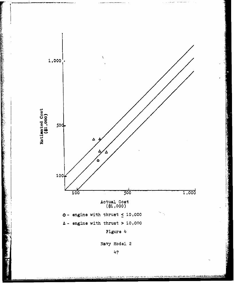
'V 0- engine with thrust < 10,000
A- engine with thrust > I0,0o0
Figure 4
Navy Model 2
47
0 0 0 /4t
100. ... 500 1,000
Actual Cost($1,000)
•-engines with thrust < 10,000 ibs
A - engines with thrust > 10,000 Ibs
Figure 5
Navy Model 3
48
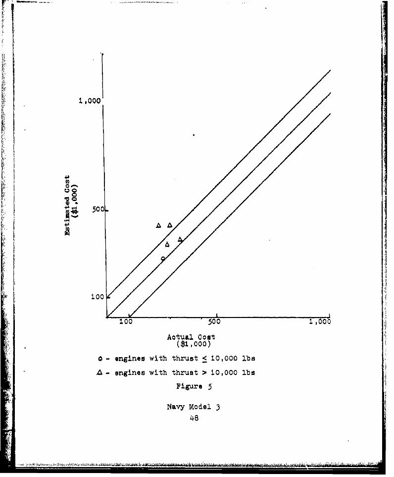
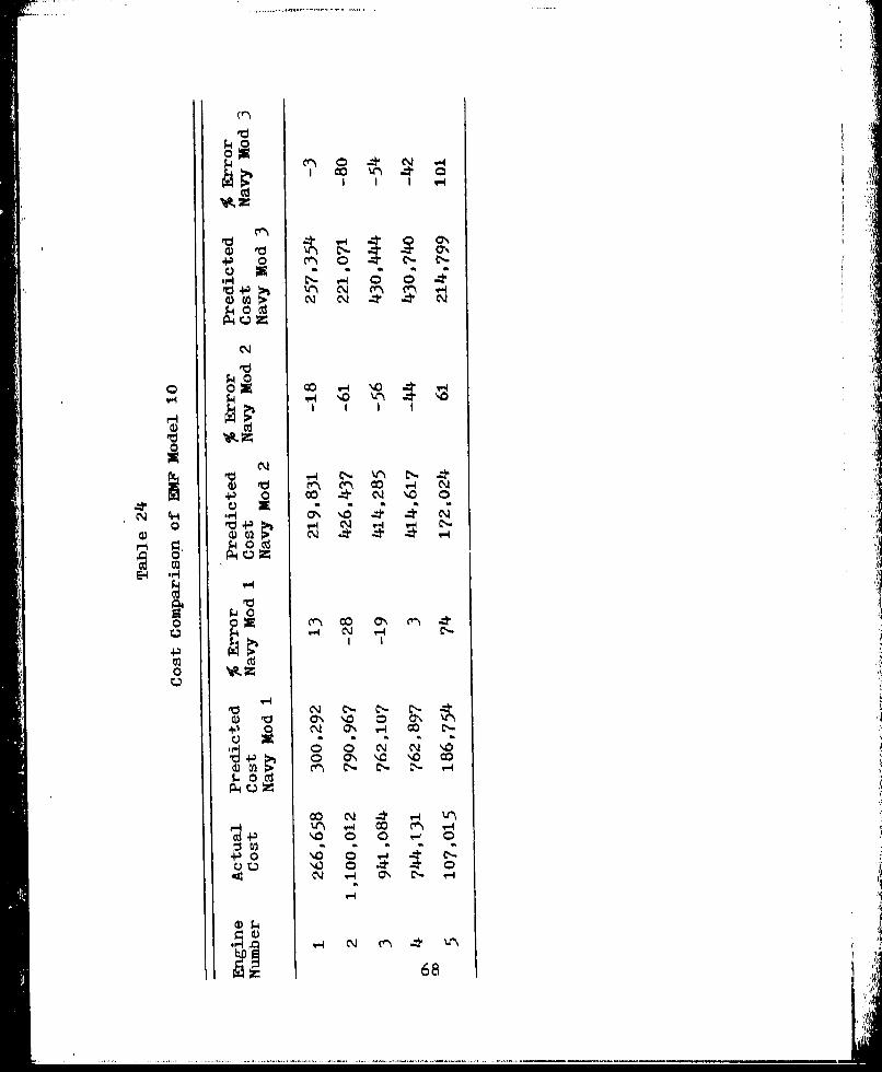
In an attempt to determine which of the three Navy
MF models was the best, it was noted that the engine thrust
or possibly the size of the MF may determine which model
gives the best results. It appeared that engines with a
maximum thrust of 0OO00 pounds or less obtained the best
results using Model 3, but that those with thrust greater
than 10,000 pounds obtained the best results using Model 2.
The MF size may also be a driving factor. In this case
Navy Model 3 performed best when the MF was less than 55,000,
and Model 2 seemed to achieve better results with a MP
above 55,000, The MF size corresponded to the amount of
thrust. Engines with a MP of less than 55,000 also had less
than 10,000 pounds of thrust. Those with a MI' greater than
55,000 had more than 10,000 pounds of thrust.
Estimated Maurer FactorModels
Overview. The objective was to develop an estimated
Maurer Factor (EMF) model which could be used in the early
development stage of a turbine engine. This section
describes the EMF models that were developed. The discussion
includes a description of the data bases, a statistical
analysis of selected models, and the results of the
validation of the models.
Model development, The EMF models were developed
using the multiple regression technique (Appendix D). The
4~9
•-OU
regression was performed using four data bases hereafter
referred to as the Basic Data Base, the Grumman Parameters
Data Base, the Turbofan Data Base, and the Turbojet Data
Base, The following is a description of the contents of
each data base.
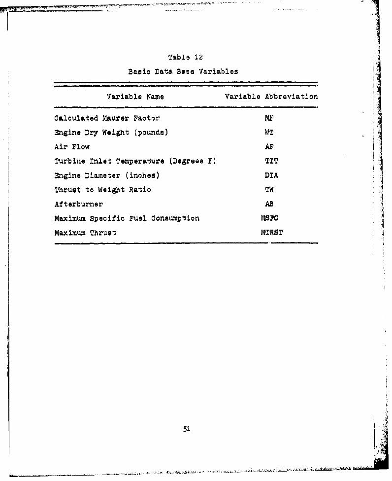
Basic-Data Base. The Basic Data Base consisted of
the calculated IF and engine parameters for 35 turbine
engines. The data for these engines were obtained from
research conducted by Mullineaux and Yanks, from analysts
at the Naval Air Development Center, from the Air Force
Gray Book, and from the Navy version of the Air Force Gray
Book. Table 12 is a summary of the variables in the Basic
Data Base.
Grumman Parameters Data Base. The GrummanParameters Data Base contained the calculated MF and some
of the engine parameters used in the Grumman cost model
discussed in Chapter 2. The Grumman Parameters were
selected because of roesearch conducted in which it was
determined that the Grumman model yielded the best cost
estimation results as compared to the Rand and Mullineaux
and Yanks models (17). Fifteen engines were used in this
data base, Table 13 is a summary of the variables in the
Grumman Parameters Data Base,
Turbofan and Turbojet Data Base. The Turbofan and
Turbojet Data Bases were developed by separating the engines
50
______ -i+•... .. .. .. .- , -•L .• I i ....'..
Table 12
Basic Data Base Variables
Variable Name Variable Abbreviation
Calculated Maurer Factor MF
Engine Dry Weight (pounds) WT
Air Flow AF
Turbine Inlet Temperature (Degrees F) TIT
Engine Diameter (inches) DIA
Thrust to Weight Ratio TW I IAft erburner AB
Maximum Specific Fuel Consumption MSPC
Maximum Thrust MTRST
51
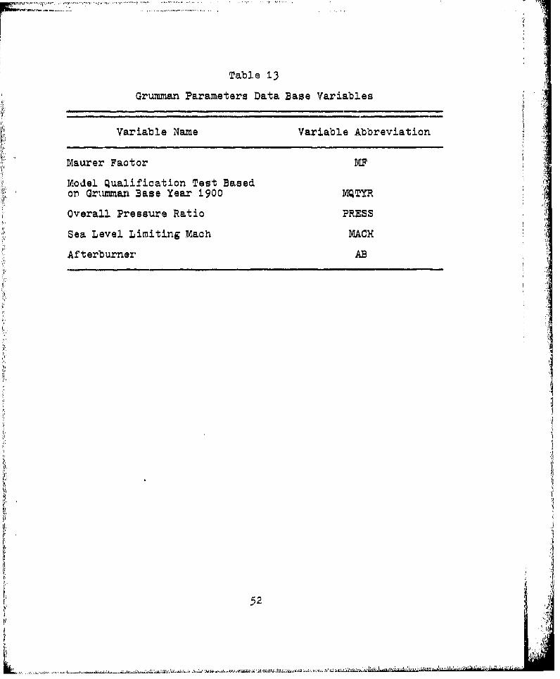
Table 13
Grumman Parameters Data Base Variables
Variable Name Variable Abbreviation
Maurer Factor Ml,
Model Qualification Test Basedor Grumman Base Year 1900 MQTYR
Overall Pressure Ratio PRESS
Sea Level Limiting Mach MACH
Afterburner AB
I
iI
52
I ....... ........
in the Basic Data Base into two categories--turbofan and
turbojet. The parameters in the Basic Data Base were also
used in the Turbofan and Turbojet Data Bases. The Turbofan
Data Base contained 11 engines and the Turbojet Data Base
contained 24 engines,
Statistical Analysis
Overview. A statistical analysis of the EMF models
was conducted to determine which models were statistically
i significant. The statistical significance of a model is
determined by measuring the dependence of a variable on a
, set of independent variables. A subjective determination
of the level of significance for each EMP model and its
independent variables was set at the a = .05 level
(2 91 243 -245),
As presented in Chapter 3, the technique of multiple
regression was used to develop the EMP models, With the
aid of a computer subprogra", REGRESSION, 13 initial models
were developed. The subprogram produced a printout with the
information required to analyze each model and its independent
variables. With this printout, it was then determined that
all models except Model i1 were statistically significant at
the a = ,05 level. Once each of the 13 models was tested
for significance, the independent variables were analyzed
as to their significance in their particular model. (See
Appendix D for further details,) After the analysis of
53
. . I I'............ .... .......-. ,i••i'•'.. ." ":i'........ / * I I.r . I* . j.I '
the overall models and the individual variables was
completed, the next step of the analysis was performed.
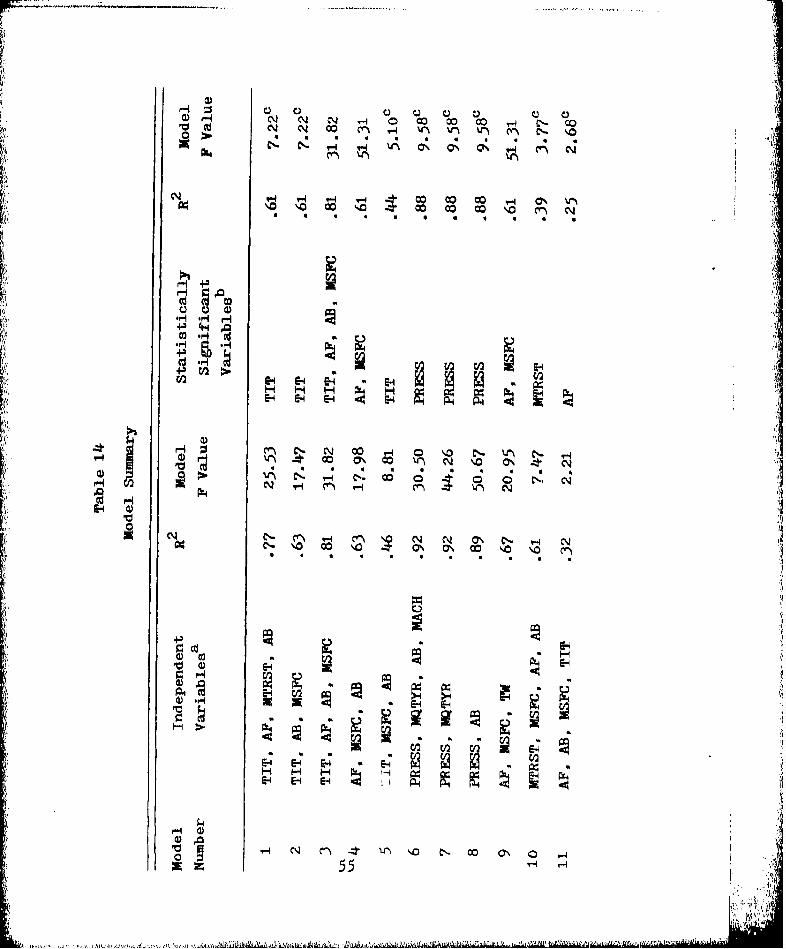
Each of the independent variables was analyzed for
significance in its EMP model. The 13 EMF models were then
run through the multiple regression subprogram, but with
this run only the previously determined significant variables
were included. Table 14 is a summary of the results of the
two-step statistical analysis. The table includes the R2
value and the F value for the overall models with all
independent variables included, The table also shows the
R2 and the F value for the same models with the statistically
insignificant independent variables excluded.
The EM' models were grouped according to the data
base used to develop the model. The following is a
discussion of the results of the statistical tests performed
on the final EMF models--that is the models with only the
significant variables included, Of particular interest was
the R value for the overall model, the F value for the
overall model, and the t statistic for the individual
variable coefficients.
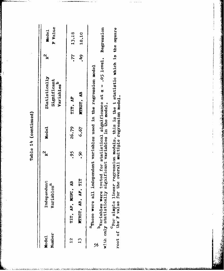
Basic Models, The Basic EMF models (Models t, 2, 3,
4, 5, and 9) which were developed using the Basic Data Base
are summarized in Table 15. The models and the independent
variables were tested for statistical significance at the
S= ,05 level, All of the final EMF models shown in Table 15
were significant as were the independent variables.
54
CD~
q- . 0 CO) 0 0 O 0qC- cm .N UN V, 0U )~ C'
vO COCOQ
.3 44 Q
4.3
.1E-4
;3C N CO '.4 0 0 C,- ul N
Nq n N NCON NN q- No
E~4-2
EE EH ~ ~ c N N 0
N ~ ~ ~ c V; % 0 ~~0~E-41 E4 4 4 4 4
1-ý H i ,
4., I-I
a) c
TE4 nEv-
55
10 1:0
c~co
4J4 4-1.
N~O \Q
oj dO) 0
100
Jt -I F-4'
q-4 W.-q
CH U.14 --I'm ~
4)2rý ~~ .H P-A4
~9"4 l-.
5 6 *i 00
..........
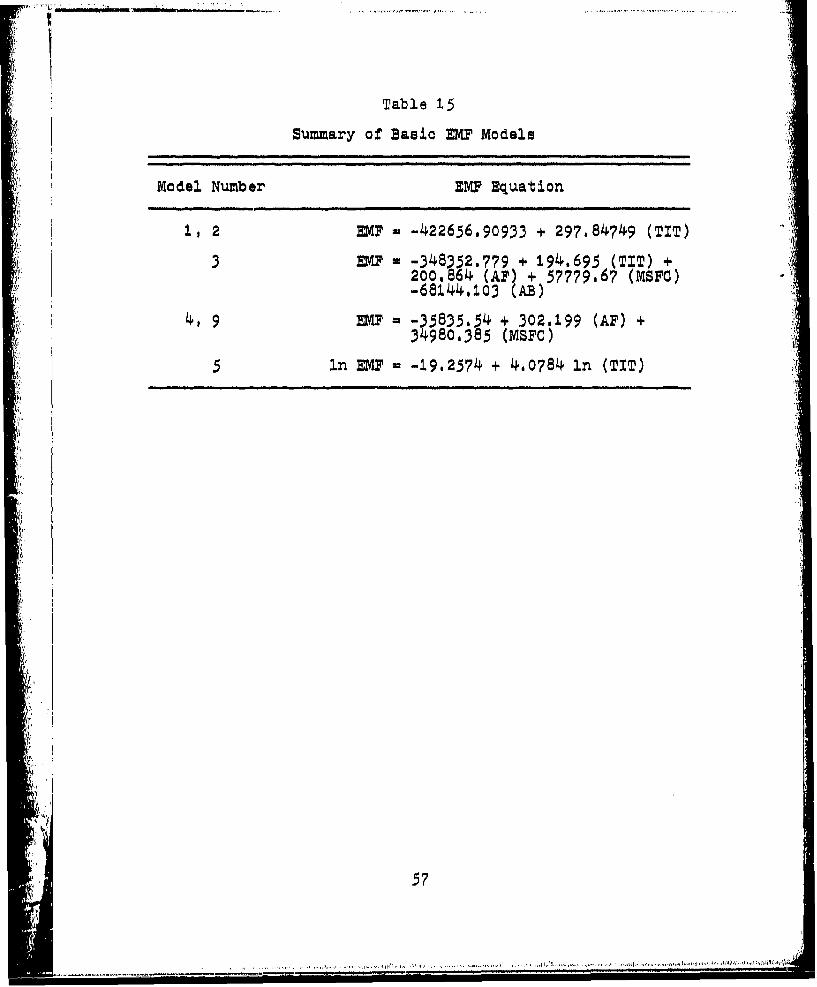
Table 15
Summary of Basic EM? Models
Model Number EMP Equation
1, 2 EMP w -422656.90933 + 297.84749 (TIT)
3 EM? = -348352.779 + 194.695 (TIT) +200.864 (AF) + 57779-67 (MSFc)-68N44.103 (AB)
4, 9 EM? a -45835.54 + 302.199 (AF) +34980.385 (MSFC)
5 in EM = -19.2574 + 4.0784 in (TIT)
57.
5?
, • . ... , ' '•i ..... ... • .....~~ ', *'', .......... ..... .. ..-
The R value in a multipie regression model is used
as an indicator of the strength of the model. It was
believed that the EMF models should have an R2 of at least
.80. Of the Basic EMF models, only Model 3 met the .80
criterion. Because of the low A2 of Models 1, 2, 41, and 5,
their use as an estimator of turbine engine costs was
questionable.
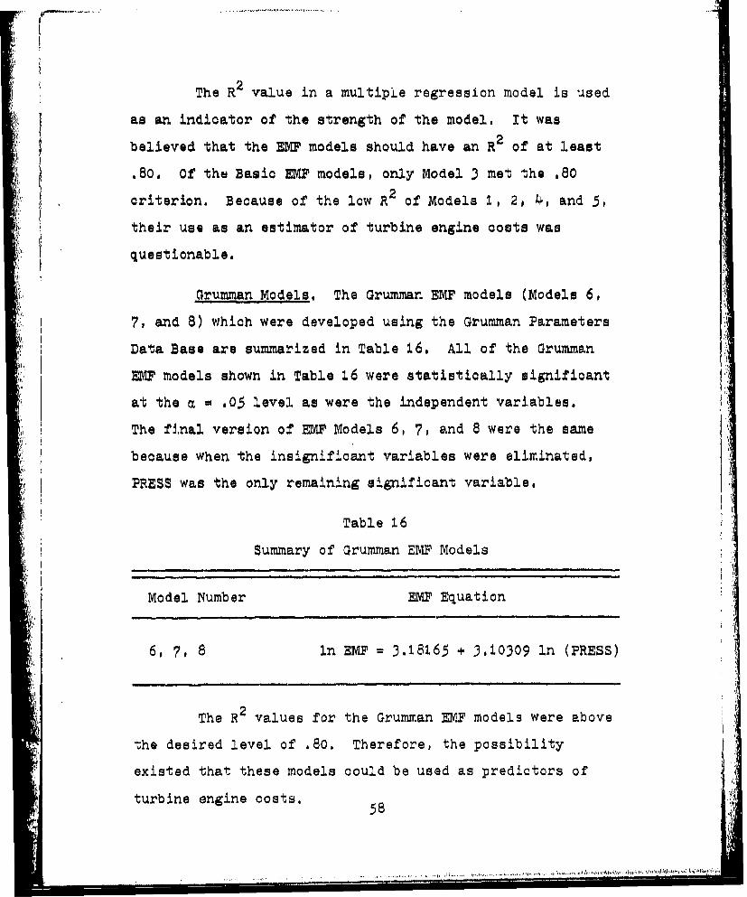
Grumman Models. The Grumman EMF models (Models 6,
7, and 8) which were developed using the Grumman Parameters
Data Base are summarized in Table 16. All of the Grumman
EMP models shown in Table 16 were statistically significant
at the m = .05 level as were the independent variables.
The final version of EMF Models 6, 7, and 8 were the same
because when the insignificant variables were eliminated,
PRESS was the only remaining significant variable.
Table 16
Summary of Grumman EMF Models
Model Number EMF Equation
6, 7, 8 ln EMF = 3.18165 + 3.10309 ln (PRESS)
The R2 values for the Grumman EMF models were above
the desired level of .80. Therefore, the possibility
existed that these models could be used as predictors of
turbine engine costs, 58
58
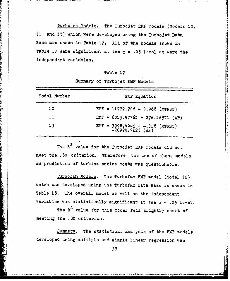
Turbojet Models. The Turbojet EMF models (Models 10,
11, and 13) which were developed using the Turbojet Data
Base are shown in Table 17, All of the models shown in
Table 17 were significant at the a = .05 level as were the
independent variables.
Table 17
Summary of Turbojet EMF Models
Model Number EMF Equation
1.0 EMFI 11777.726 + 2.968 (MTRST)
II mF - 6015.97761 + 276.16571 (AF)
13 DIF = 3998.4245 + 4.318 (MTRST)-20990,7223 (AB)
2i
The R2 value for the Turbojet EMF models did not
meet the .80 criterion. Therefore, the use of these models
as predictors of turbine engine costs was questionable,
Turbofan Models. The Turbofan EMP model (Model 12)
which was developed using the Turbofan Data Base is shown in
Table 18. The overall model as well as the independent
variables was statistically significant at the a = .05 level.
The R2 value for this model fell slightly short of
meeting the .80 criterion.
Summary. The statistical ana-'ysis of the EMF models
developed using multiple and simple linear regression was
59
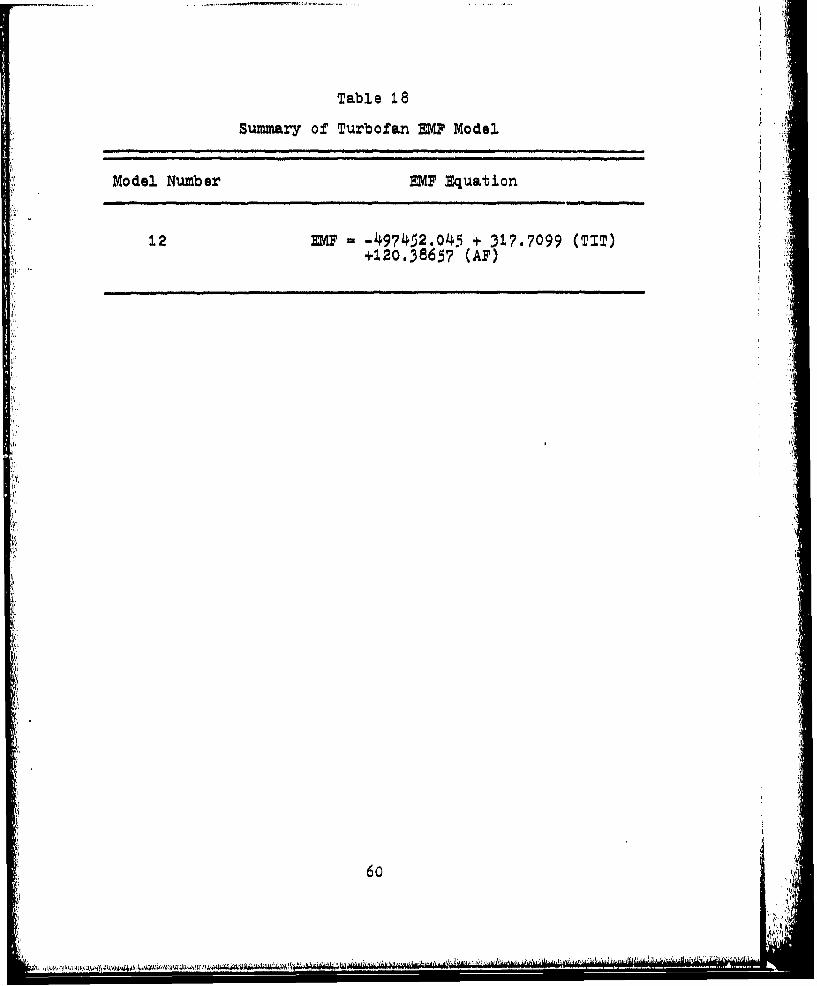
Table 18
Summary of Turbofan EvP Model
Model Number vMF Equation
12 EP= -4974.2.o45 + 317.7099 (TIT)+120.3865? (A?)
6o
.t
* . .1. . .
performed to determine which of the models were statistically
significant. The desired R2 level and the a level were
subjectively selected by the researchers so that the
relative statistical strength of the different EMP models
could be determined,
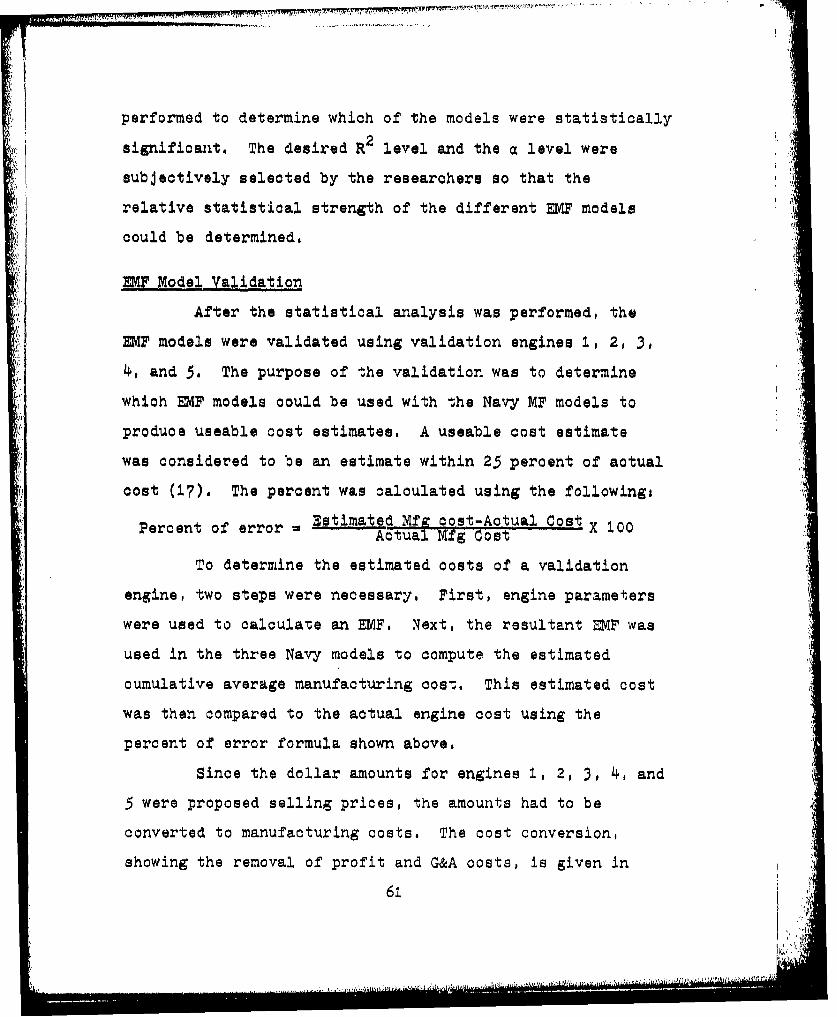
EMP Model Validation
After the statistical analysis was performed, the
EMF models were validated using validation engines 1, 2, 3,
4, and 5. The purpose of the validation was to determine
which EMF models could be used with the Navy MF models to
produce useable cost estimates, A useable cost estimate
was considered to be an estimate within 25 percent of actual
cost (17). The percent was calculated using the following,
3stimated Mfg cost-Actual CostPercent of error = Acul•gCs•X tooActual Mfg cost
To determine the estimated costs of a validation
engine, two steps were necessary. First, engine parameters
were used to calculate an EMF. Next, the resultant EMF was
used in the three Navy models to compute the estimated
cumulative average manufacturing cost. This estimated cost
was then compared to the actual engine cost using the
percent of error formula shown above.
Since the dollar amounts for engines 1, 2, 3, 4, and
5 were proposed selling prices, the amounts had to be
converted to manufacturing costs. The cost conversion,
showing the removal of profit and G&A costs, is given in
61"I ............. .
Appendix E. Also the costs for the engine controls and
accessories were removed from the total engine cost, There-
fore, all costs in the next section are the cumulative
average manufacturing costs of engines without controls and
accessories in PY78 dollars,
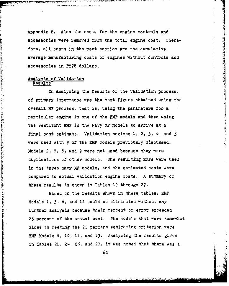
Analysis of ValidationResults
In analyzing the results of the validation process,
of primary importance was the cost figure obtained using the
overall M? process, that is, using the parameters for a
particular engine in one of the EWF models and then using
the resultant EMF in the Navy MP models to arrive at a
final cost estimate. Validation engines 1, 2, 3, 4, and 5
were used with 9 of the EMW models previously discussed.
Models 2, 7, 8, and 9 were not used because they were
duplications of other models. The resulting EMFs were used
in the three Navy MF models, and the estimated costs were
compared to actual validation engine costs. A summary of
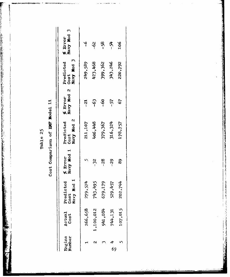
these results is shown in Tables 19 through 27.
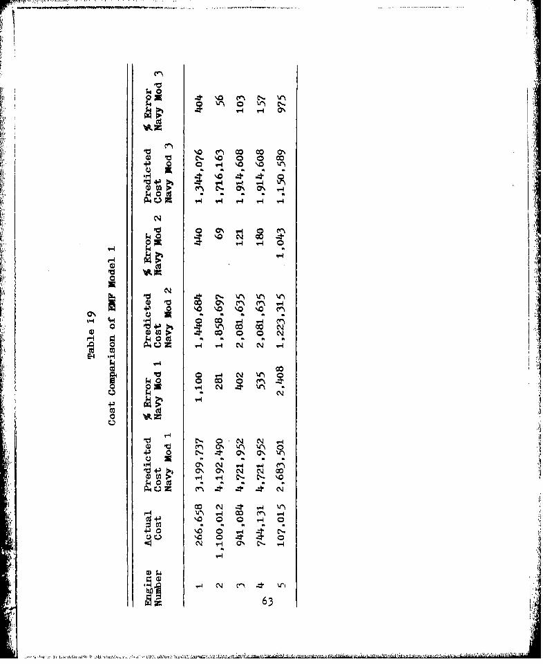
Based on the results shown in these tables, EMF
Models 1, 3, 6, and 12 could be eliminated without any
further analysis because their percent of error exceeded
25 percent of the actual cost. The models that were somewhat
close to meeting the 25 percent estimating criterion were
EMF Models 4, 10, 11, and 13. Analyzing the results given
in Tables 21, 24, 25, and 27, it was noted that there was a
62
.: . ... ..... .. .... i
IVI
N .,o c0 0. v-
Pw4
ON 0 4~ O W
14 '. -0
ON V
14` 0%4 CO44 - - -4 0
....... .Q ...
~.P4
4-1 N N
90 4- 000
4-1O
0
4- 0 10 4 N 0N ~- C~-N ~. .ON H
MA6
coN 0
v-4
r44 0r
"-4 I I I4
0 0
N C
+1 a C 0' 0
+3 0
'~O N65
Ilk
'.0 4J'. r- C.4) 03 ~ O ~
0 ON C'~N ON
V O C- N '.0 \Y~0
I C-ý Cý c4
0O \
- C-- a \
~0 0E-44
b.0
z 66
04-
PO4) r O V' ca
0 N as a o
vC-4 C v-4
FO ~ 0- cl N C
4"4Ifn
0N
0- 0 N a' '0
00
N ~ O ~ C
~ F ~ ~ ,- C0
4 1 a
C.) E a - a a7
... 0. ..0.....
kt 0 0 - -
0 00
V.. 100
N~- "04 0%044
mm0/
o N • , ,•
Li i68
N C-
0 V- Cz '-4
0.) ON 0' 1.0 0 aN
0. 0 N ,N~
U' v-4 CO n -4-3 0 0 V- 0
4) 0~4 C-
N (-4 ON Cs. -
468
00 N
CE q-4 co 0 C'-
C- C') c.-
V4w
C-4 CH-
SN ON ON
N C Nl
00
CO n
~ '4~ % N .4
.H '-4 0% n- VI
0z 69 ~ .. .
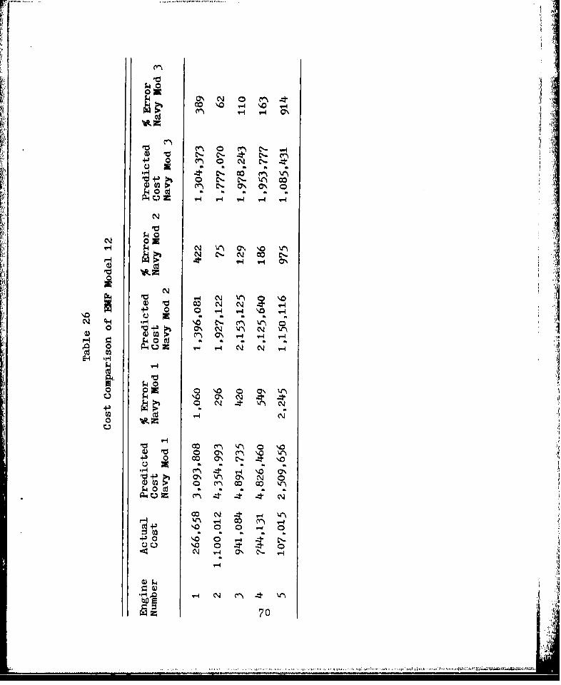
C- 0 co -
P400 C-. CI-cm N' aN
v- - -4 9-1 -
~C\ V - -
NN
FO 4. N Ewn C'-N -4 " "-
00
EH -
N~C - N~
4-3N 4-
I; lii' 0 ca aa
ND 0 0
5V.4 N -4
40
Az 70
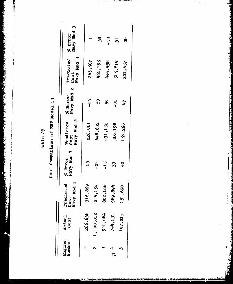
VI V)i
NNC
C144 4..
'0 4- 3 o- - N
O' :4a. a
(I r-q
oc 0n~
p' 0
iIN o\ N
4-
- a a 71
pattern in the percentage of errors for the different engines
using the 3 Navy MF models. As was done previously with the
ME' validation, a comparison between the percent of error and
engine thrust was made in an attempt to explain the pattern
that existed. IEngines 2, 3, and 4 had a thrust greater than 25,000
pounds. Engine I thrust was less than 10,000 pounds but was
very similar to the engines in the data base. Engine 5
thrust was also less than 10,000 pounds but was very much
smaller than engines in the data base.
Although engine 5 had a percent of error of I using
EMP Model 4 and Navy MF Model 2, EMF Model 4 was the only
model where engine 5 obtained results that were less than
the 25 percent criterion, Since this was the only case
where engine 5 came close to the 25 percent criterion, it
was decided that the cost of engines of the same type as
engine 5 (very small engines with thrust well below 10,000
pounds) could not be determined using the EMF models.
Engine 1, which was considered to be a conventional
size engine with less than 25,000 pounds of thrust, met the
25 percent criterion for E/F Models 4, 10, 11, and 13 using
all 3 Navy models with one exception--EMF Model 4, Navy
Model 2. Therefore, it appeared that EMF Models 4, 10, 11,
or 13 could be used with any of the Navy models to estimate
the manufacturing cost of a turbine engine with less than
25,000 pounds of thrust. However, the overall best results
72
.... . ... ....
were obtained when these EMF models (Models 4, 10, 11, or
13) were used with Navy M? Models I or 3.
For engines 2, 3, and 4, which all had thrusts
greater than 25,000 pounds, the 2.5 percent criterion was met
in most cases using EMP Models 4, 10, and 13 and Navy MF
Model 1. The beet overall results for engines 2, 3, and 4
were obtained using EMW Model 4 and Navy MP Model 1.
The analysis of the validation results of the EPF
models indicated that some models yielded unuseable cost
estimates while other models had results that met the 25
percent estimating criterion. Based on engine thrust,
generalizations were made as to what types of engines should
"be used with the EM1 models and the Navy MF models. It
was suggested that,
1. The EIF models cannot be used for very small
engines (such as engine 5 where the thrust is well below
10,000 pounds).
2. EKF Models 4, 10, 11, or 13 and Navy MF Models 1
or 3 yield results which meet the 25 percent estimating
criterion for conventional size engines with less than25,000 pounds of thrust.
3. EMP Model 4 in conjunction with Navy M? Model 1
yielded the best results for engines with thrust greater
than 25,000 pounds.
However, before it could be stated that th-se EMF
models can be used to estimate turbine engine costs, the
73
results of the statistical tests of these EMF Models had to
be considered. Of importance were the statistical signi-
ficance of the overall model, the statistical significance
of the individual regressors, the model R2 value, and the
possibility of autocorrelation in the data, As previously
discussed, the final EMF models were shown to be significantas were the individual regressors (Table 14).
Although EMP Models 4, 10, 1i, and 13 met the 25
percent estimating criterion, it could not be stated with
confidence that these same results would be obtained with
other engines because of the low R2 value of these models.
Due to the limited size of the data base, it was believed
that a R of at least .80 was required for the EMP models.
E!1 Models 4, .0, 11, and 13 did not meet the .80 criterion
Another factor that should be considered when dealing
with regression models is autocorrelation in the data base,
Autocorrelation indicates the presence of a relationship
among the residuals; thus, "with positive autocorrelation,
the second (or some later) observation tends to resemble, or
repeat the first observation, and hence gives little new
information [29,626]." The result of autocorrelation is
that the estimated regression line is shifted farther from
the true regression line. This shift causes the regression
constant to be overestimated and the regressor coefficients
to be underestimated or vice vlrsa, depending on whether the
estimate is above or below the true regression line, The
74
amount of error is dependent on how much the independent
variable of the item being estimated varies from the mean
of the independent variable in the data base. The problem
with autooorrelation is not that it biases the estimate,
since an overestimate is as likely as an underestimate,
Rather, the problem is that the estimate may be badly wide
of the target (29s627).
Autocorrelation in the data was determined by using
the Durbin-Watson statistic, To perform the test, the
independent variable of interest was ordered, and then the
multiple regression subprogram was used to obtain the
Durbin-Watson statistic. This statistic was compared to
Durbin-Watson critical values obtained from a Durbin-Watson
statistic table (29t720-721). The computer program used to
order the data is given in Figure 9 Appendix D. (See
Appendix D for detailed explanat'on of the Durbin-Watson
test.)
Using the Durbin-Watson test, it was determined that
all EMF models except Model 10 were developed using auto-
correlated data.
The existence of autocorrelation was important for
two reasons. First, it was stated previously that EMF
Models 4, 10, Ilp and 13 yielded results which met the
25 percent estimating criterion. However since Models 4,
ii, and 13 had autocorrelation, these models should not be
used as cost estimators, Because of autocorrelation, the
75
..........
Lq
acceptable results obtained using the validation engines
does not guarantee the same results if other engines are
used in the models.
The other MOF models (Models 1, 2, 3, 5, 6, 7, 8, 9,
and 12) yielded cost estimates that did not meet the 25
percent estimating criterion. It was believed that auto-
correlation was the cause of the gross estimates resulting
from these models.
Summary, The analysis of the validation results
indicated that EMF Models 4, 10, 11, and 13 met the 25
percent estimating criterion. The remaining models did not,
However, further statistical analysis of EMF Models 4, 10,
11, and 13 suggested that Models 4, 11, and 13 should not
be used as cost estimators because of the presence of
autocorrelation. EMF Model 10 met the 25 percent criterion
and was not developed from autocorrelated data. However,
the R2 value for Model 10 did not meet the .80 criterioni
therefore, Model 10 should not be used as an estimator.
Based on the foregoing analysis, it was concludedthat all of the EMF models were unreliable and should not
be used to estimate turbine engine costs.
Answers To ResearchQuestions
Research Question 1. What steps are necessary to
develop and use the Maurer Factor cost estimation model?
. . .
A detailed explanation of the steps involved in the
MF technique is given in Appendix C.
Research Question 2, What results can be achieved
concerning turbine engine cost estimation in the early
development stage by using the Maurer Factor cost estimation
e6 8,mfemodel?
The Maurer Factor was computed for validation
, engines It 6, 7, 8l and 9, The computed MF for these engines •
was then used in the three Navy MF models. According to
expert opinion, the results of parametric cost models are
"considered good if the resultant estimate is within 25
percent of actual cost (17). As shown in Table 11 and
Figures 4 and 5, this 25 percent criterion was met by
validation engines 1, 6, and 9.
Research Question 3. Is the learning curve appli-
cable in turbine engine cost estimation?
It was believed that 'the use of learning curve theory
is essential in turbine engine cost estimation. The learning
curve was used to adjust the actual cost of engines to some
basis--that basis being the cumulative average cost per
engine based on 1500 engines,
In their thesis, Mullineaux and Yanks have stated
that learning curve theory should not be applied to turbine
engine production because of the production lot system that
is used by engine manufacturers, However, the researchers
77-..
F
and experts in the turbine engine field believe that some
learning does take place regardless of what production
methods are used (7M 17). The manufacturers of the
validation engines used in this thesis all use some form
of learning curve (1?).
In stating that learning curve theory does apply to
turbine engine production, caution must be used when
selecting an average percent of learning that can be applied
to all engines and all manufacturers. As shown in Appendix
B, where the percent of learning for different engines was
computed, different engines have different learning curves.
Also, as shown in Table 9, different engine manufacturers
use different curves.
In summary, the cost analyst using learning curve
theory as part of the cost estimation process, must be able
to determine which learning curve is appropriate for a
particular manufacturer and a particular engine.
Research Question 4. How can the learning curve be
incorporated with the Maurer Factor technique?
In this study, learning curve computations were used
to adjust all engine costs to the cumulative average cost
of 1500 engines. This is the main application of learning
curve theory in conjunction with the MF technique (7).
Using the Navy MF models, the estimated cost
obtained is the cumulative average cost of an engine based
on production of 1500 engines. Using a learning curve, this
78
cost can be adjusted to the engine cost based on any desired
cumulative number of engines, The cost can also be adjusted
to the unit cost of an engine based on any n th unit of that
engine produced. However, before any of these cost
adjustments can be made, the percent of learning for the
particular manufacturer must be known (7).
Research Hypothesis
I A model based on engine performance parameters can
be developed which will estimate the Maurer Factor,
Several EMF models were developed, and all were
shown to be statistically significant, Although several of
the WMI models met the 25 percent criterion, it was shown
I that these models should not be used as turbine engine costI2
estimators because of the low model R2 and autocorrelation,
STherefore with the available data, it was determined that
a useable EMF model could not be developed.
* 7Ii
Chapter 5
CONCLUSIONS AND RECOMENDATIONS
Overview
As stated in Chapter 1, a cost estimating model is
needed which can be used to estimate the cost of a turbine
engine early in its development stage. This chapter contains
the conclusions related to the analysis of one such technique
discussed in previous chapters--the Maurer Factor (MF) cost
estimating technique.
One objective of this thesis was to analyze the MF
cost estimating technique. The analysis included,
I. A look at what steps were necessary to use the
MF cost estimating technique.
2. What results could be obtained using the MF
technique,
3. Some of the problems encountered using the MF
technique.
The conclusions in this chapter are based on the analysis
and on some of the problems encountered in attempting to use
the MF technique.
Another area of research was devoted to developing
a regression model that could be used to estimate the Maurer
Factor, This estimated Maurer Factor (EMF) could be used
in conjunction with the Navy MF models to estimate the cost
80
............i
of a turbine engine, The conclusions for this portion of
the research are based on the statistical analysis and the
validation results of the EMW models.
Finally, based on the findings concerning the MF
technique, some recommendations are presented.
Conclusions
Maurer Factor technique. In analyzing the MF
technique, the steps required to use the technique, the
results obtained using the technique, and the problems
encountered using the technique were considered. The
following results were obtained,
To use the MF technique, the MF for a particular
engine was calculated. This process included tasks ranging
from breaking down an engine into its individual components
to determining the gross weight of the individual components,
A step-by-step procedure explaining this process is given in
Appendix C.
After it was determined that the MF for an engine
could be calculated, the cost estimating results using the
three Navy MF models (Table 10) were evaluated, The model
was considered to be useable if the cost estimate was
within 25 percent of the actual engine cost (17). To keep
the validation of the MF technique unbiased, validation
engines were selected which had not been used in developing
the Navy MF cost models. The MF for the validation engines
81
I
was calculated and used with the three Navy MF models. The
results showed that the 25 percent estimating criterion
could be met, depending on which engine was used with a
particular Navy model. Based on the validati. results
(Table 1i), it was concluded that the MF technique could be
used and would yield cost estimates that met the 25 percent
estimating criterion. Also, based on the validation results,
it was concluded that engines with a maximum thrust of less
than 10,000 pounds obtained the overall best results using
Navy MF Model 3 (Table 10). For engines with a thrust value
greater than 10,000 pounds, Navy MF Model 2 achieved the
best results. Although the estimating criterion was met
using the validation engines, it should be noted that the
MF validation process was based on a limited number of
validation engines,
Several problems were encountered during the
validation of the MF cost estimating technique. These
problems included a lack of data required to calculate the
MF and the questionable currency of the MF weighting factors
(Table 5). The following is a discussion of these problems.
A small number of validation engines was used
because the data required to compute the MF for an engine
was not available, To calculate the MF, the gross weight
and type of material of each engine component must be known,
The information is contained in the DD Form 3 46 which should
be supplied by the engine manufacturers. However, the form
82
. .....' . , . '. ......, . •
....... ............
has not been supplied in most insta es, and as a result, it
was impossible to calculate the MF.
Another problem in obtaining the weight information
occurred even when the manufacturers did supply the
information. Many times manufacturers did not koiow the
actual gross weight of a component before machining, When
this occurred, the manufacturers had to estimate the gross
weight. For validation engine I, the manufacturer supplied
the data required to calculate the MF, and several of the
component weights were estimated.
Another problem was encountered with the MF
weighting factors. The weighting factors are used to
introducA a difficulty of machinability factor into the MF
calculation, The difficulty factor is based on the
hardness of different materials. What is not taken into
consideration in the weighting factors is the drastic
increase in the prices of some materials (7). Although
price increases due to inflationary pressures were
compensated for by using price index adjustments (Appendix A),
the price Increase for some materials is much greater than
current inflation rates. As a result, the accuracy of the
MF technique will probably be affected in the future if
some method is not found to compensate for rapidly rising
materials prices.
Estimated Maurer Factor models. As discussed
throughout this thesis, it was difficult to obtain the data
83
.~ ~ ~ ... .. ...... .......................
necessary to calculate the MF. The gross weights of the
individual engine components were often not available
because the manufacturer had not provided them. Another
reason that the data may not be available is because the
engine is in a stage of development where specific details
about engine components are not known. However, since the
MF cost estimating technique did meet the 25 percent
estimating criterion as shown in Chapter 4, it was decided
to develop a regression model that would estimate the MP.
This estimated Maurer Factor (EMP) could then be used with
the Navy MF models to estimate the cost of a turbine engine.
The following conclusions were based on the
statistical analysis and validation of the EMF models.
1. A high R value does not always indicate the
predictive capability of a model. Several of the initially
developed EMP models had an R2 value greater than .90.
However, further analysis indicated that many of the
independent variables were insignificant. These variables
did nothing for the overall model except increase the R
value by insignificant amounts. Validation attempts using
these initial models resulted in gross estimating errors
because of the inclusion of the insignificant variables,
When the insignificant variables in the initial
EMF models were removed, the R2 values dropped. However,
model validation showed that several of these final models
with low R2 values in the range of .25 to .65 achieved the
84L
L• V
22
best estimating results. (See Table 1,L and Tables 21, 2LJ,
25, and 27.) Therefore, the R value alone should not be
used to analyze the predictive capability of a model.
2. The data used to develop a model should be tested
for autocorrelation. When several of the EWI models
achieved large estimating errors in the validation process,
the data was tested for autocorrelation. The test results
indicated that autocorrelated data had been used to develop
all but one of the EMF models. Therefore, some of the models
which achieved acceptable results in the validation process
could not be used with any reasonable level of confidence.
3. Of the 13 MVF models developed, Model 10 was the
only model that was void of autocorrelation problems and
still met the 25 percent estimating criterion, It was
concluded that EMF Model 10 should be used in conjunction
with Navy MF Models I or 3 when estimating the costs of
engines with less than 25,000 pounds of thrust. For engines
with more than 25,000 pounds of thrust, EMF Model 10 should
be used in conjunction with Navy Model 1. For very small
engines, the EMF models should not be used.
4, Although EMF Model 10 met the 25 percent
estimating criterion, confidence in its predictive capability
was limited because of its low R2 value. If the model had2
been developed using a larger data base, a low R value would
be more acceptable. Also, confidence in EMF Model 10s
predictive capability was limited because of the small
number of engines used in the validation process,• .• 85
Recommendations
The recommendations are based on the results of
analyzing the validation of the Maurer Factor cost estimating
technique. As previously mentioned, one problem encountered
in validating the MF technique was lack of data necessary
to compute the MF. Therefore, it is recoin r&1Ad that the
DD Form 346 be mandatory for engine contr.'ts. This form
would enable cost analysts to obtain the gross weights of
engine components which are required to compute the MF.
Another problem mentioned was the rapidly increasing
prices of raw materials used to build turbine engines, As
a possible area for future study, it is recommended that
an attempt be made to include a factor in the MF cost
estimating process which will compensate for rapidly
increasing prices.
Finally, it is recommended that an effort be
directed toward increasing the size of the data base used
to develop EMP Model 10. The enlargement of the data base
should include more modern, advanced technology engines,
Copies of the data bases used in this thesis may be obtained
from the authors or from Richard McNally, AFAPL/TBP,
Wright-Patterson AFB, Ohio.
In conjunction with increasing the data base size,
it is recommended that further validation of EMF Model 10
should be accomplished. It is believed that if increased
confidence in EMF Model 10 could be developed, the effort
86
would be beneficial. The research indicated that the Maurer
Factor technique is a feasible technique which can meet the
25 percent estimating criterion, but the data required to
calculate the MP is not always available. Therefore, a
model which could be confidently used to estimate the MF
would make the use of the Maurer Factor cost estimating
technique more applicable.
In view of increasing defense costs and the
decreasing buying power of the defense dollar, effective
cost estimating techniques are an important part of defense
planning and decision making. It has been the objective
of this thesis to contribute in some way to improving cost
estimating techniques.
87.
87a
*
I I I
APPENDIX A
INDlEX NUMBERS
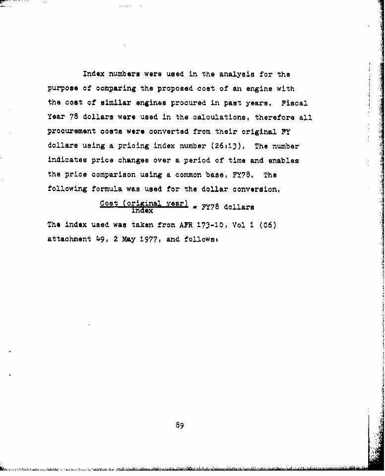
Index numbers were used in the analysis for the
purpose of comparing the proposed cost of an engine with
the cost of similar engines procured in past years. Fiscal
Year 78 dollars were used in the calculations, therefore all
procurement costs were converted from their original FY
dollars using a pricing index number (26,13). The number
indicates price changes over a period of time and enables
the price comparison using a common base, FY78. The
following formula was used for the dollar conversion.
cost (original Year) . FY78 dollarsindex
The index used was taken from AFR 173-10, Vol 1, (06)
attachment 49, 2 May 1977, and followst
89
. ., ..~ ..- ......... .....
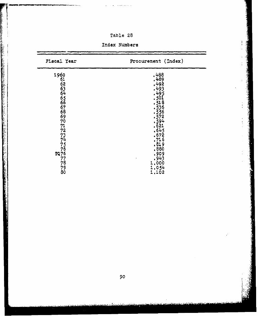
Table 28
Index Numbers
Fiscal Year Procurement (Index)
196o .48861 .48962 ,492
63 .,49364 .49565 .50166 .51.867 53668 .55669 .57270 59471 :621272 .64574. 672.
75 .8•976 .880TQ76 .909 ,77 .94378 . 00079 1.05480 . 102.02
90
r'

APPENDIX B
LEARNING CURVE
91.
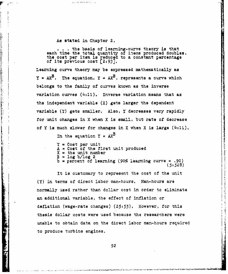
As stated in Chapter 2,
the basis of learning-curve theory is thateach time the total quantity of items produced doubles,the cost per item is reduced to a constant percentageof its previous cost C21933.
Learning curve theory may be expressed mathematically as
Y a AXB* The equationo Y = AXB, represents a curve which
belongs to the family of curves known as the inverse
variation curves (4,11). Inverse variation means that as
the independent variable (X) gets larger the dependent
variable (Y) gets smaller. Also, Y decreases very rapidly
for unit changes in X when X is small, but rate of decrease
of Y is much slower for changes in X when X is large (4tii),
In the equation Y AXB
Y = Cost per unitA = Cost of the first unit producedX = the unit numberB = log b/log 2b = percent of learning (90% learning curve = .90)(51526)
It is customary to represent the cost of the unit
(Y) in terms of direct labor man-hours. Man-hours are
normally used rather than dollar cost in order to eliminate
an additional variable, the effect of inflation or
deflation (wage-rate changes) (25l55). However, for this
thesis dollar costs were used because the researchers were
unable to obtain data on the direct labor man-hours required
to produce turbine engines.
92
""I 4
To compensate for the effect of inflation on turbine
engine costs, all costs used in the learning curve compu-
tations for this thesis were adjusted to base year 1978
dollars. (See Appendix A for discussion on the use of price
index numbers.)
There are two learning curve cost models. Cne model,
called the "unit curve" or "Boeing" theory was validated by
the Stanford Research Institute study (25,50). The unit
curve model expresses cost as unit cost. The other learning
curve model is the "Northrop" model, which bases cost on
the cumulative average cost per unit (24).
In this thesis, cumulative average learning curve
theory was used to compute the cumulative average cost of
the validation engines.
Since the Navy's MF cost estimation models were
based on the average cost of 1500 engines, the costs of the
validation engines used in this thesis were adjusted to the
cumulative average cost per unit of 1500 engines.
The following is a discussion of how the cumulative
average cost of an engine based on the cumulative average
cost of 1500 engines was determined. The percent of learning
for a particular engine had to be determined. The Gray
Book was used to determine (1) in what year a certain engine
was produced, (2) the numbers of that engine produced in a
year, and (3) the average cost of the engines in a
93
i,, (ALI.
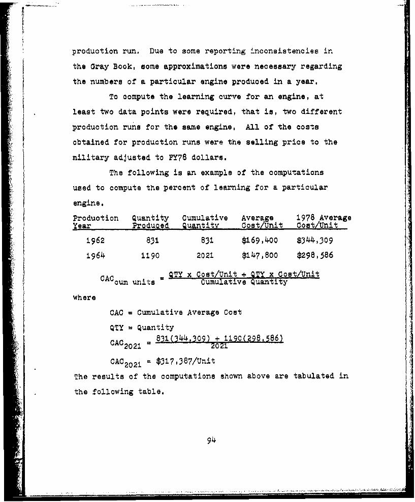
production run. Due to some reporting inconsistencies in
the Gray Book, some approximations were necessary regarding
the numbers of a particular engine produced in a year.
To compute the learning curve for an engine, at
least two data points were required, that is, two different
production runs for the same engine. All of the costs
obtained for production runs were the selling price to the
military adjusted to FY78 dollars.
The following is an example of the computations
used to compute the percent of learning for a particular
engine.
Production Quantity Cumulative Average 1978 AverageYear Produced Quantity Cost/Unit Cost/Unit
1962 831 831 $169,400 $344,309
1964 1.190 2021 $147,800 $298,586Aoum units QTY x Cost/Unit + QTY x Cost/Unit
cum units Cumulative Quantity
where
CAC = Cumulative Average Cost
QTY = Quantity831(344,309) + 1.190(298,586)
2021 2021
CAC 20 21 $317,387/Unit
The results of the computations shown above are tabulated in
the following table.
94
.. .. .. .... .
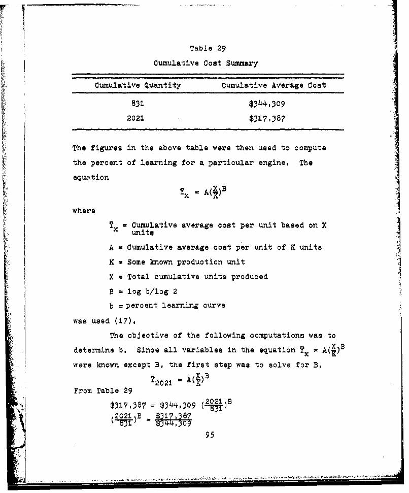
Table 29
Cumulative Cost Summary
Cumulative Quantity Cumulative Average Cost
831 $344,3o9
2021 $317,387
The figures in the above table were then used to compute
the percent of learning for a particular engine. The
equation
= A("B
where
= Cumulative average cost per unit based on Xunits I.
A = Cumulative average cost per unit of K units
K X Some known production unit
X = Total cumulative units produced
B = log b/log 2 41
b = percent learning curve
was used (17).
The objective of the following computations was to
determine b. Since all variables in the equation ? =
were known except B, the first step was to solve for B.
?2021 A(X)From Table 29
$317,387 = $344,309 2021 B-B31'
2021B $317,387
95
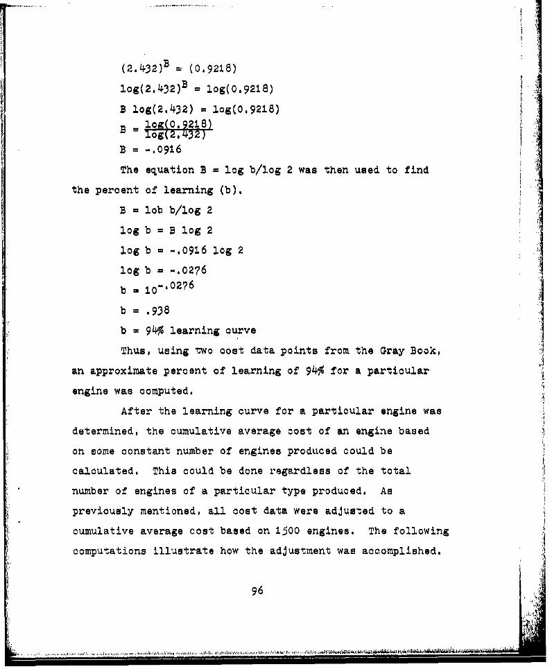
(2.432)B = (0.9218)
log(2.432)B = log(o.9218)
B log(2.432) - log(O.9218)
B lo zg(2. •32)
B = -. 0916
The equation B = log b/log 2 was then used to find
the percent of learning (b).
B = lob b/log 2
log b = B log 2
log b = -. 0916 log 2
log b = -. 0276
b - 1o-0276
b - .938
b = 94% learning curve
Thus, using two cost data points from the Gray Book,
an approximate percent of learning of 94% for a particular
engine was computed.
After the learning curve for a particular engine was
determined, the cumulative average cost of an engine based
on some constant number of engines produced could be
calculated. This could be done regardless of the total
number of engines of a particular type produced. As
previously mentioned, all cost data were adjusted to a
cumulative average cost based on 1500 engines. The following
computations illustrate how the adjustment was accomplished.
96
... ... I. ....
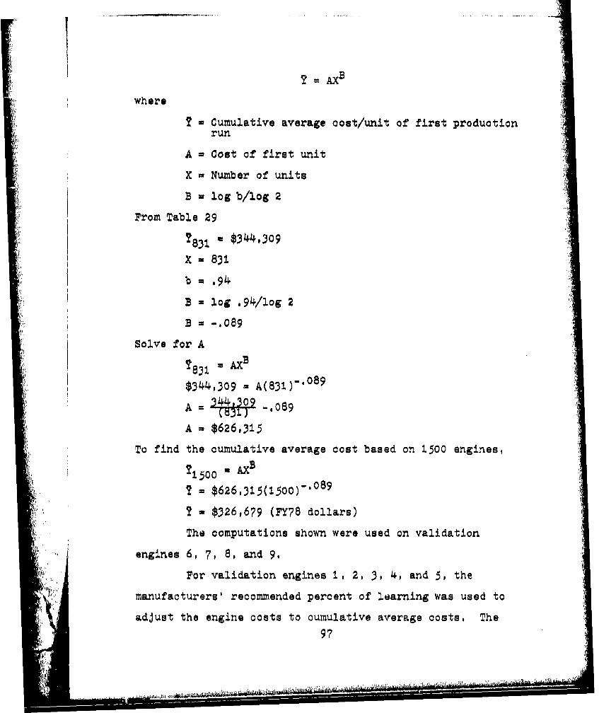
?=AX B
where
S,- Cumulative average oost/unit of first productionrun
A = Cost of first unit
X - Number of units
B log b/log 2
From Table 29
2831 U $344,309
X = 831
b ..94
B = log .94/log 2
B = -. 089
Solve for A
2831 0 AX.
$344,309 = A(831)"' 0 8 9
A 344,09 .089
A = $626,315
To find the cumulative average cost based on 1500 engines,
?1500 = AX3
. $626'315(1500)-'089
2-$326,679 (PY7B dollars)
The computations shown were used on validation
engines 6, 7, 8, and 9.
For validation engines 1, 2, 3, 4, and 5, the
manufacturers' recommended percent of learning was used to
adjust the engine costs to cumulative average costs. The
97
method of computing the cumulative average cost of engines
1, 2, 3, 4, and 5 varied for the different engines, there-
fore a brief explanation of the computation foreach engine
is given. Since the calculations for engine I were the most
complex, this procedure is discussed first,
The standard method used to compute cumulative
average cost per engine based on a cumulative average cost
of 1500 engines was shown in the first part of this appendix.
However, another method had to be used to compute the
cumulative average cost for validation engine ±.
The proposed actual cost to the Air Force of a new
advanced engine was obtained through the Propulsion Branch
AFAPLI This engine was used as one of the validation
engines for the different cost estimation models in this
thesis. The cost was known for the total engine and was
also broken down into the cost of the basic engine and the
engine accessories, The proposed actual cost was based on
the cumulative average cost per unit of the first 50 engines
produced (17).
To make a valid comparison of validation engine
actual cost to validation engine estimated cost using the
various M? cost estimating models, the proposed actual cost
of the validation engine had to be adjusted to the
cumulative average cost per engine based on 1500 engines.
The manufacturer producing the validation engine
believed that the cumulative learning curve behaves somewhat
98
. ....
differently than the Northrop learning curve, The manu-
facturer produced engines in lots of 50. They believed
that cumulative average costs should be computed for each
production lot of 50 engines, and this computation must be
performed for each lot of 50 engines until the cumulative
quantity of engines equals the desired cumulative basis of
1500 engines. However, the cumulative average cost per
engin, for the first 50 engines remains in the equation for
all computations. The total cost for each lot was computed
based on the cumulative average cost for each lot, and the
summation of the computations was divided by 1500 to obtain
the cumulative average cost per engine.
The equation A(•) was used for the computations
where
YX cumulative average cost per unit based on X
units
A - known average cost of first production lot of 50engines
X = cumulative quantity of engines (50 unitincrements)
X = number of engines per production lot (K = 50)
ii B w log b/log 2 (Manufacturer uses 90% learning)
99
..... ......
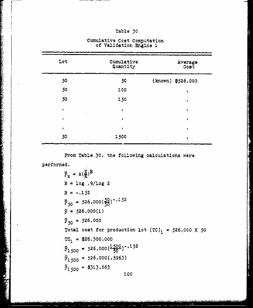
Table 30
Cumulative Cost Computationof Validation Engine I.
Lot Cumulative AverageQuantity cost
50 50 (known) $526,000
50 100
50 150
50 1500
From Table 30, the following calculations were
performed,
B = log .9/log 2
B= -.152
Y50 = 5260000( Y 152
y= 526,000(1)
=5 526,000
Total coat for production lot (TC), 526,000 X 50
TC1 $26,300,000
Y150 =1o 526,000(.5963)
lOO= $313,663ý1100
TC3 0 3 513,663 X 50
TC3 0 = $15,683,151
Using the same computations as shown above, the cumulative
average cost based on 1500 engines can be found by using the
equation S30
91500 = 1 , Ta
The calculations just shown were accomplished by
computer using the program shown in Figure 6. The program
was designed to compute the cumulative average cost per unit
based on 1500 engines. The program can be used to determines
1. the cost of the total engine (basic + controls)
2, the cost of the basic engine
3. the cost of the controls.
The standard learning curve computations discussed
earlier were used to accomplish the cumulative average cost
adjustment for validation engines 2, 3, and 4, However,
engine 5 required a slight variation of the standard
learning curve computation.
For validation engine 5, the manufacturer used two
different percents of learning. The engine cost was
separated into a basic cost and two different types of
labor cost. The following computations were used to
compute the cumulative average cost of engine 5,
-1500 Basic Cost + AI(X)B1 + A2(x)B2
where
101
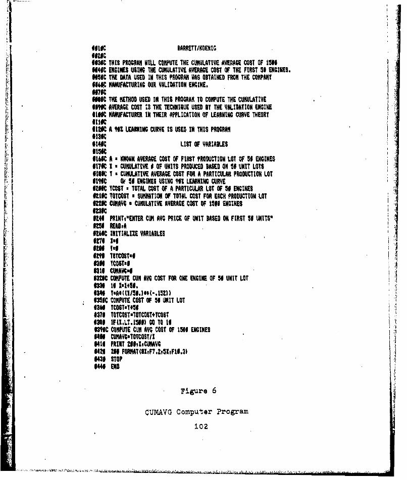
ifto BARRETTIKOENIG
003fC THIS PROGRAM VILL COMPUTE THE CUMULATIVE AVERAGE COST OF 1510U4C ENGINES USING THE CUMULATIVE AVERAGE COST OF THE FIRST 51 ENGINES.005IC THE DATA USED IN THIS PRORAAN VAS OBTAINED FROM THE COKPANTI", MANUFACTURING OUR VALIDATION ENGINE.
WN THE METHOD USED I THIS PROGRAM TO COMPUTE THE CUMULATIVE1I1W AVERAGE COST 04 THE TECHNIQUE USED It THE VALIDATION ENGINEIWOC MANUFACTURER IN THEIR APPLICATION OF LEARNING CURVE THEORTlueKf120C A 96% LEARNING CURVE IS USED IN THIS PROGRAM113K114K LIST OF VARIABLESDISKIL4C A a KNOON AVERAGE COST OF FIRST PRODUCTION LOT OF 51 ENGINES617K 1 v CUMULATIVE I OF UNITS PRODUCED BASED ON 50 UNIT LOTS
01CK 1 a CUMULATIVE AVERAGE COST FOR A PARTICULAR PRODUCTION LOTOIfC OF 51 ENGINES USING 901 LEARNING CURVEOZffC YCOST x TOTAL COST OF A PARTICULAR LOT OF 50 ENGINESOZIOC TOTCOST, SUMMATION OF TOTAL COST FOR EACH PRODUCTION LOTWIZC CUHAVG * CUMULATIVE AVERAGE COST OF 1500 ENGINES
0240 PRINT,"ENTER CUR AVG PRICE OF UNIT BASED OH FIRST 51 UNITS"I510 READ,A
IM TOTCOST',
0300 YCOSTIOA10l CUKAVG.03IlC COMPUTE CUR AVG COST FOR ONE ENGINE OF S0 UNIT LOT
0331 If Is4.l.03401 'A(1115.)4'('.15Z)).13WIC COMPUTE COST OF 50 UNIT LOT1310 TCOSTr.*#50370 TOTCOSTTOTCOST+TCOST0381 IF(I.LTSOO) GO TO If1CK COMPUTE CUM AVG COST OF 1500 ENGINES
1410 CUNAVG'TOTCOST/I014 PRINT 110ObCUMAVG042I 200 FORNT(1,F1.2414,FI1.3)1430 STOP0441 END
Figure 6
CUMAVG Computer Program
102
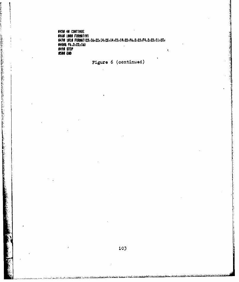
145f 46 CONTINUE04049 1 FQIMFRATMY6470 IltI FORNAT(21di6,21dt4,Udi4,Zlt4,ZXF4.2Z,1F4.ZZdlZXtl94661 F6.3oZXI4l#4"9 STOP6569 END
Figure 6 (oantinued)
103
1500= cumulative average cost/unit based on 1500
engines
Al a labor cost of first engine
A2 - labor cost of first engine
Bi w log bj/log 2
bi - percent of learning for different labor types
X r number of engines
bi= .90
b 2 .85
B= log .90/log 2
BI -. 152
B2 log .85/log 2
B2 -. 234
= 71,293 + 262,092(1500)"' 1 5 2 + 55,416(1500)"' 2 3 4
?1500 $167,539
104~,

APPENDIX C
MAURER FACTOR TECHNIQUE
105
The following is a step-by-step explanation of the
procedure used to estimate the cost of validation engine I1
using the MF technique. The steps include engine component
breakdown, materials classification, MP calculations, and
determination of the final estimated cost.
Component Breakdown
Each individual component in the validation engine
was identified, and the gross weight of the material used
to make the component was determined. The component data
are available on the DD Form 346s (Table 7) supplied by
engine contractors, The component data for the validation
engine were supplied by the engine manufacturer (Table 31).
Material Indexing
Using the Aerospace Material Specification (AMS)
index, an AMS number was assigned to each material type
MF Classification
The materials were classified using the seven MF
categories (Table 32). The classification was accomplished
by using the AMS conversion table shown in Table 33 and the
data are shown in Table 34. The purpose of the MF
categorization was to enable assignment of the MF weighting
factor (fj).
106
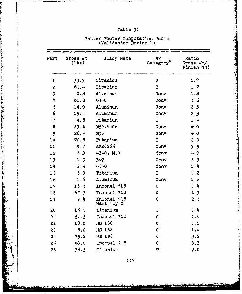
Table 31,
Maurer Factor Computation Table(Validation Engine 1)
Part Gross Wt Alloy Name MF Ratioa(lbs) Category (Gross Wt/Finish Wt)
1 55.3 Titanium T 1.7
2 65.4 Titanium T 1,7
3 0.8 Aluminum Cony 1.2
4 61.8 4340 Cony 3.6
5 14.0 Aluminum Conv 2.36 19.4 Aluminum Conv 2.3
7 4.8 Titanium T 1,4
8 23.2 M50,440c Cony 4.09 26.4 M50 Conv 4.o
10 72.8 Titanium T 2.011 9.7 AMS6265 Cony 3.512 8.3 4340, M50 Conv 4.013 1.9 347 Cony 2.3
14 2.9 4340 Cony 1.4
15 6.o Titanium T 1.216 1.6 Aluminum Conv 1.2
17 16,3 Inconel 718 C 1.4
is 67.7 Inconel 718 C 2.319 9.4 Inconel 718 C 2.3
1.astoloy X
20 15.5 Titanium T 1.4
21 51,5 Inconel 718 C 1.422 18.0 HS 188 C 1.123 8.2 HS 188 C 1.4
24 752 FTS 188 c 3,2
25 43.0 Inconel 718 C3.326 38.5 Titanium T 7.0
107
......................................................... .. 1 - - r...
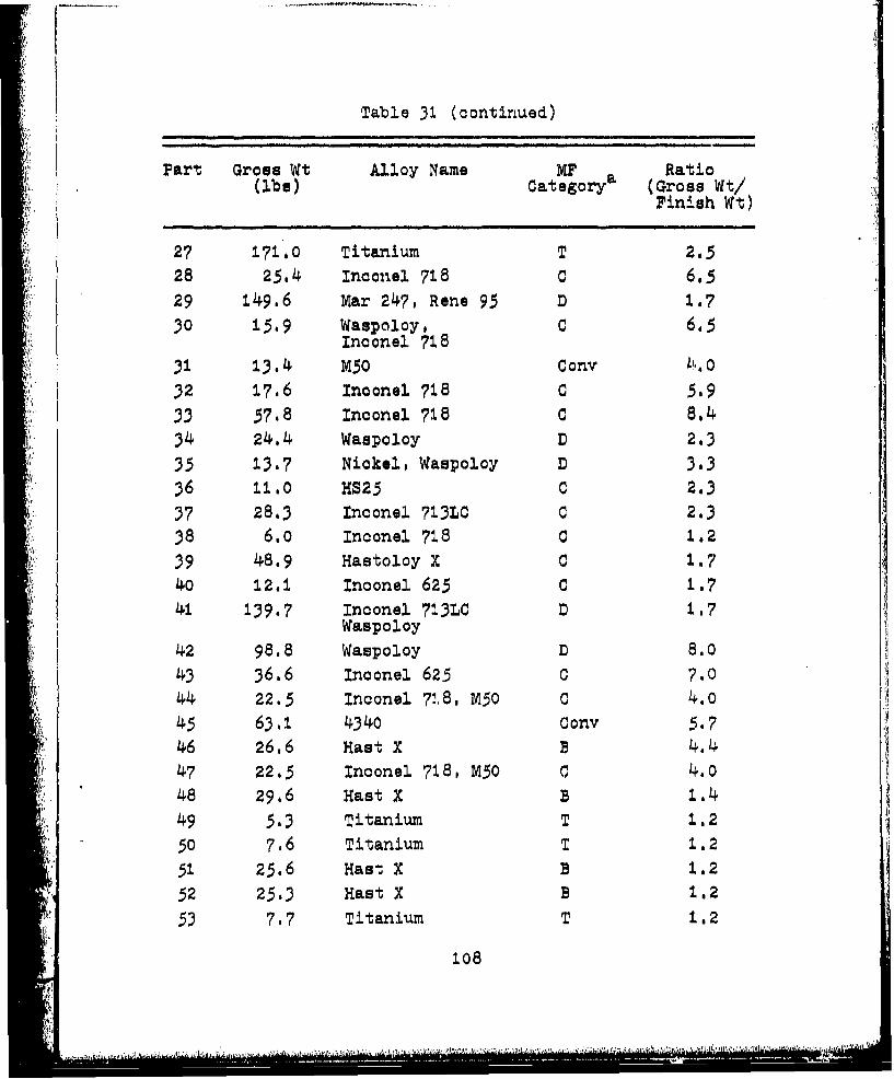
Table 31 (continued)
Part Gross Wt Alloy Name MF Ratio
(lbs) Category (Gross Wt/Finish Wt)
27 171.0 Titanium T 2.528 25,4 Inconel 718 C 6.5
29 149.6 Mar 247, Rene 95 D 1.7
30 15.9 Waspoloy, C 6.5Inconel 718
31 13.4 M50 Cony 0
32 17.6 Inconel 718 C 5.933 57.8 Inconel 718 C 8.434 24,4 Waspoloy D 2.3
35 13.7 Nickel, Waspoloy D 3.336 11.0 MS25 C 2.337 28.3 Inoonel 713LC C 2.338 6.0 Inconel 718 C 1.239 48.9 Hastoloy X C 1.7
40 12.1 Inconel 625 C 1.741 139.7 Inconel 713LC D 1.7
Waspoloy
42 98.8 Waspoloy D 8.0
43 36.6 Inoonel 625 C 7.0
44 22.5 Inconel 718., M50 C 4.045 63.1 4340 Conv 5.746 26.6 Hast X B 4.4
47 22.5 Inconel 718, M50 C 4.048 29.6 Hast X B 1.4
49 5.3 Titanium T 1.250 7.6 Titanium T 1.251 25.6 Hast X B 1.252 25.3 Hast X B 1.2
53 7.7 Titanium T 1.2
108
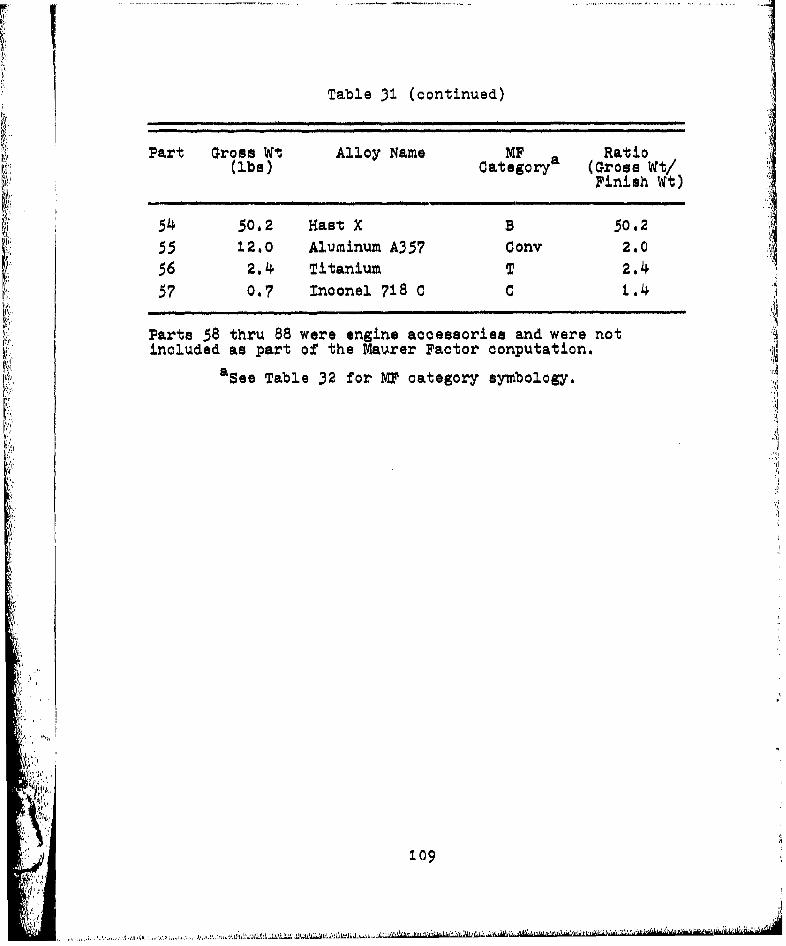
!ITable 31 (continued)
Part Gross Wt Alloy Name MF Ratio(ibs) Categorya (Gross Wt/
Finish Wt)
54 50,2 Hast X B 50.2
55 12,0 Aluainum A357 Cony 2.056 2.4 Titanium T 2.4
57 0.7 Inoonel 718 C C 1.4
Parts 58 thru 88 were engine accessories and were notincluded as part of the Matrer Factor conputation.
aSee Table 32 for MF category symbology.
log
I,'
Sl109
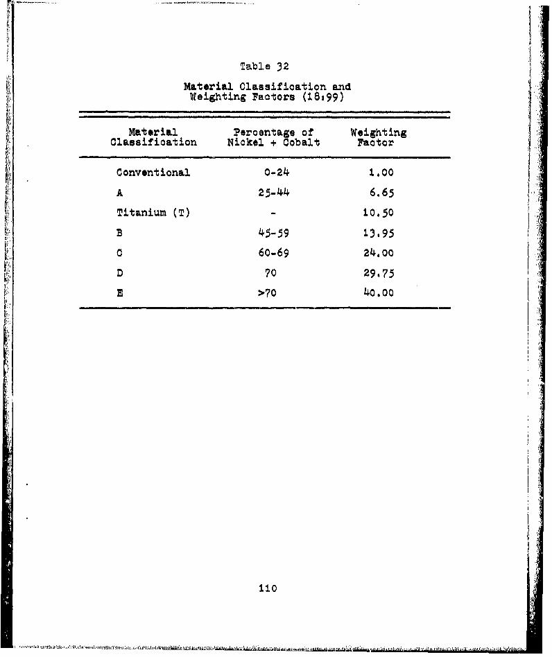
Table 32
Material Classification andWeighting Factors (18,99)
Material Percentage of Weighting
Conventional 0-24 1.00
A 25-44 6.65
Titanium (T) 10.50
B 45-59 13.95
0 60-69 24,00D 70 29-75 ,,
E >70 4o.0o
110
,,. , '-,, 'J • ', l
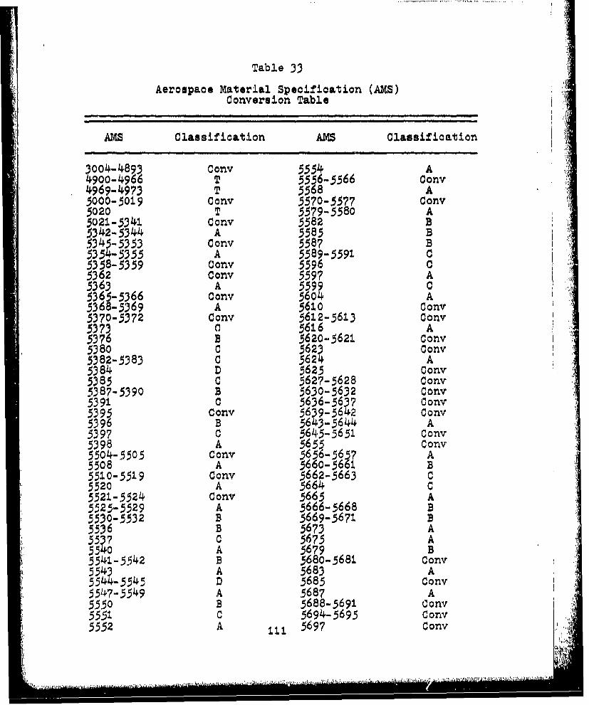
Table 33
Aerospace Material Specification (AMS)Conversion Table
AMS Classification AMS Classification
3004-4893 Cony 5554 A4900-4966 T 5556-5566 Cony4969-4973 T 5568 A5000-501.9 Conv 5570-5577 Cony5020 T 5579-5580 A5021-5341 Cony 5582 B53042-5344 A 5585 B5345-5353 Cony 5587 B5354-5355 A 5589-5591 C5358-5359 Conv 5596 C5362 Cony 5597 A5363 A 5599 C5365- 5366 Cony 5604 A5368-5369 A 5610 Conv5370-5372 Cony 5612-5613 Cony5373 C 561.6 A5376 B 5620-5621 Cony5380 C 5623 Conv5382-5383 C 5624 A5384 D 5625 Cony5385 C 5627-5628 Cony5387-5390 B 5630-5632 Cony5391 C 5636-5637 Conv5395 Cony 5639-5642 Cony5396 B 56 3-5644 A5397 C 5645-5651 Cony5398 A 5655 Cony5504-5505 Cony 5656-5657 A5508 A 5660-5661 B5510-5519 Cony 5662-5663 C5520 A 5664 C5521-5524 Cony 5665 A5525-5529 A 5666-5668 B5530-5532 B 5669-5671 B5536 B 5673 A55ý7 C 5675 A5540 A 5679 B5541-5542 B 5680- 5681 Conv
. 5543 A 5683 A5544-5545 D 5685 Conv5547-5549 A 5687 A5550 B 5688-5691 Cony5551 C 5694-5695 Cony5552 A 111 5697 Cony
'P . I I ,,.,,*j. '-F•
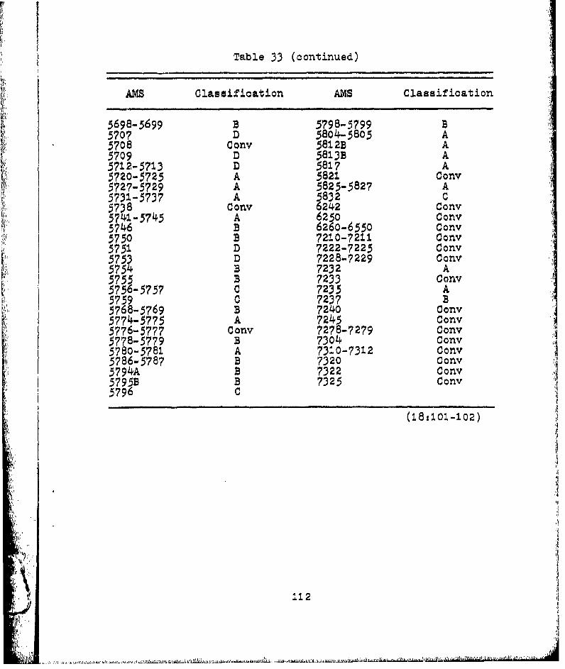
Table 33 (continued)
AMS Classification AMS Classification
5698-5699 B 5798-5799 B5707 D 5804-5805 A5708 Cony 5812B A5709 D 5813B A5712-5713 D 5817 A5720-5725 A 5821 Cony5727-5729 A 5825-5827 A5731-5737 A 58ý2 C5738 Cony 6242 Cony5741-5745 A 6250 Cony5746 B 6260-6550 Conv5750 B 7210-7211 Cony5751 D 7222-7225 Conv5753 D 7228-7229 Conv5754 B 7232 A5755 B 7233 Conv5756-5757 C 7235 A5759 C 7237 B5768-5769 B 72 0 Conv5774-5775 A 7245 Cony5776-5777 Cony 7278-7279 Conv5778-5779 3 7304 Cony5780-5781 A 7310-7312 Conv5786-5787 B 7320 Conv5794A B 7322 Conv5795B B 7325 Cony5796 C
(18,1oI-1o2)
112
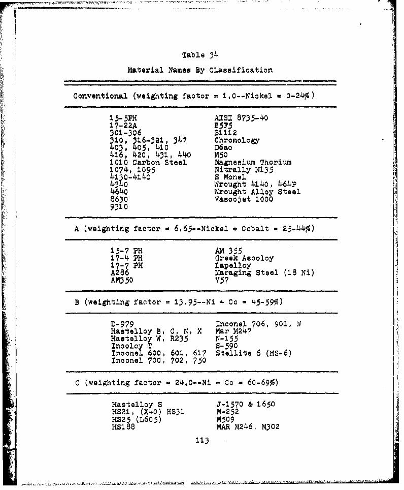
fflo.. ....... ... r
Table 34 p.
Material Names By Classification
Conventional (weighting factor = 1,0--Nickel = 0-24%)
15-51H AISI 8735-4017-22A B5F5301-306 B11124O 10 6-321, 347 Chromology
0•o5,410 D6ac416, 420, 431, 440 M501010 Carbon Steel Magnesium Thorium1074, 1095 Nitrally N135413o-4140 S Monel4340 Wrought 4140, 464P
Wrought Alloy Steel8630 Vasoojet 10009310
A (weighting factor = 6.65--Nickel + Cobalt = 25-44%)
15-7 PH AM 39517-4 PH Greek Ascoloy17-7 PH LapelloyA286 Maraging Steel (18 Ni)AM350 V57
B (weighting factor 13.95--Ni + Co = 45-59%)
D-979 Inconel 706, 901, WHastelloy B, C, N, X Mar M247Hastelloy W, R235 N-155Inooloy T S-590Inconel 600, 601, 617 Stellite 6 (HS-6)Inconel 700, 702, 750
C (weighting factor = 24.0--Ni + Co 60-69%)
Hastelloy S J-1570 & 1650
HS21, (X40) HS31 M-252HS25 (L605) M509HS188 MAR M246, M302
113
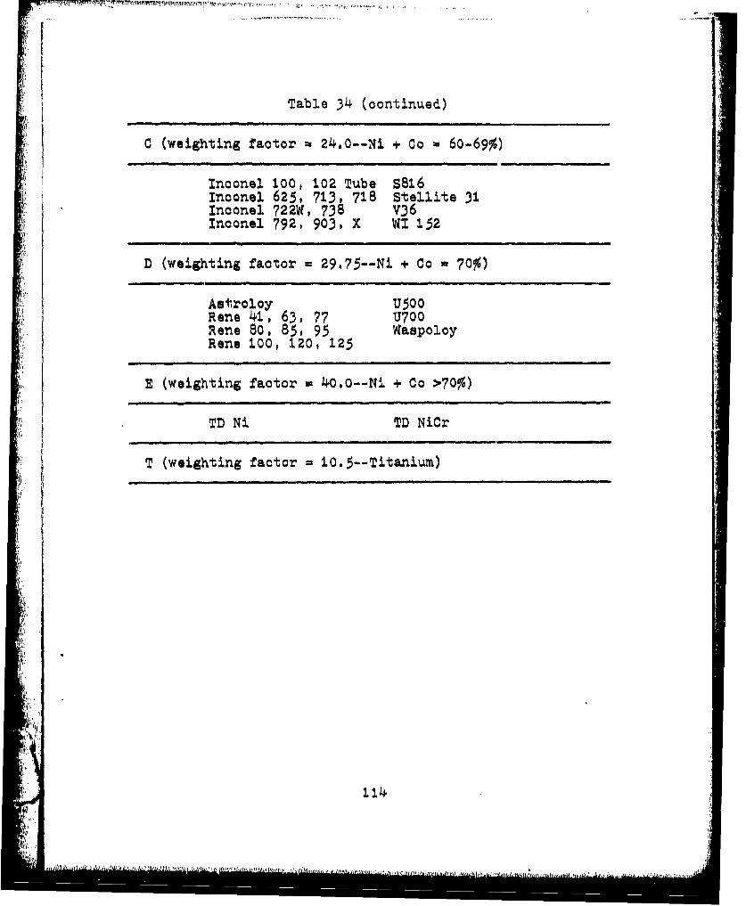
Table 34 (continued)
C (weighting factor = 2460--Ni + Co = 60-69%)
Inoonel 100, 102 Tube S816Inconel 625, 713, 718 Stellite 31Inconel 722W, 738 V36Inconel 792, 903, X WI 152
D (weighting factor u 29,75--Ni + Co 70%)
Astroloy U500Rene 41, 63, 77 U700Rene 80, 85, 95 WaspoloyRene 100, 120, 125
E (weighting factor * 40.0--Ni + Co >70%)
TD Ni TD NiCr
T (weighting factor = 10.5--Titanium)
11
1.1.4
.. U . ..- ~ ,-
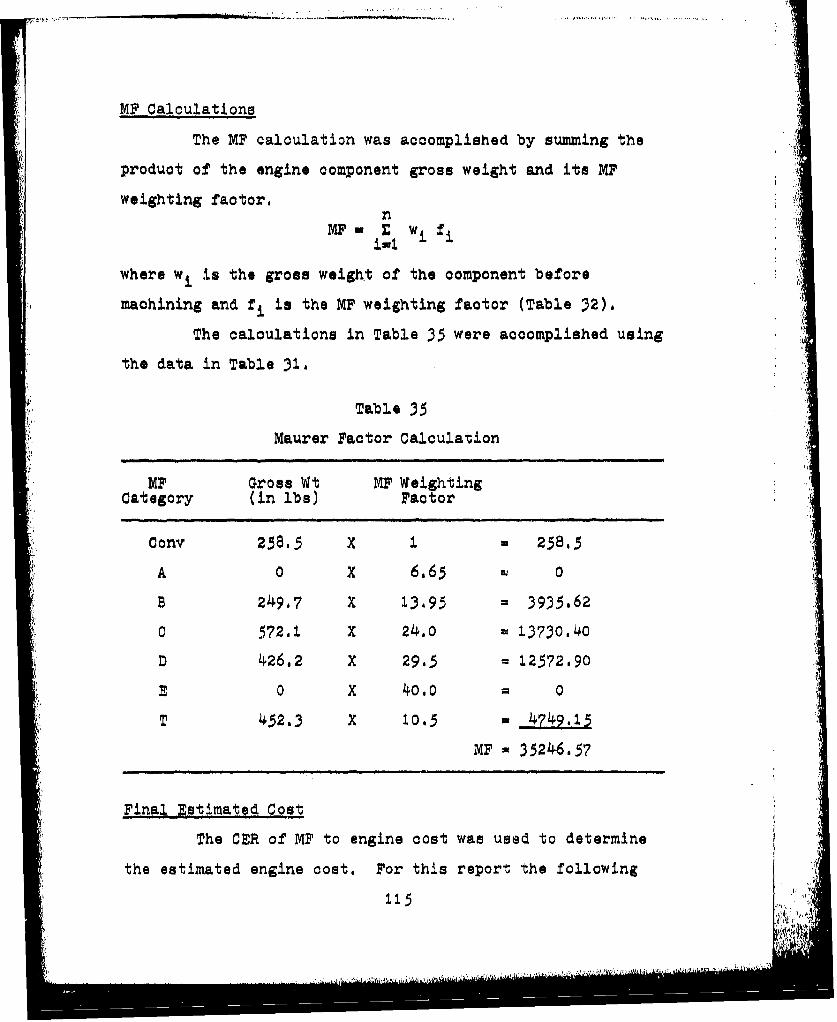
MF Calculations
The MF calculation was accomplished by summing the
product of the engine component gross weight and its MP4
weighting factor.niMF - Wj wfl
I=I.? i, ii
where wi is the gross weight of the component before
machining and f is the MP weighting factor (Table 32).
The calculations in Table 35 were accomplished using
the data in Table 31.
Table 35Maurer Factor Calculation
" IvMF Gross Wt MF Weighting
* Category (in ibs) Factor
Cony 258.5 x 1 2 258.5
A 0 X 6.65 0
B 249.7 X 13.95 = 3935.62
C 572,1 X 24.0 = 13730.40
D 426,2 X 29,5 = 12572.90
3 0 X 4o,00 0
S452.3 x 10.5 = 4749.15
MF = 35246.57
Final Estimated Cost
The CER of MF to engine cost was used to determine
the estimated engine cost. For this report the following
115
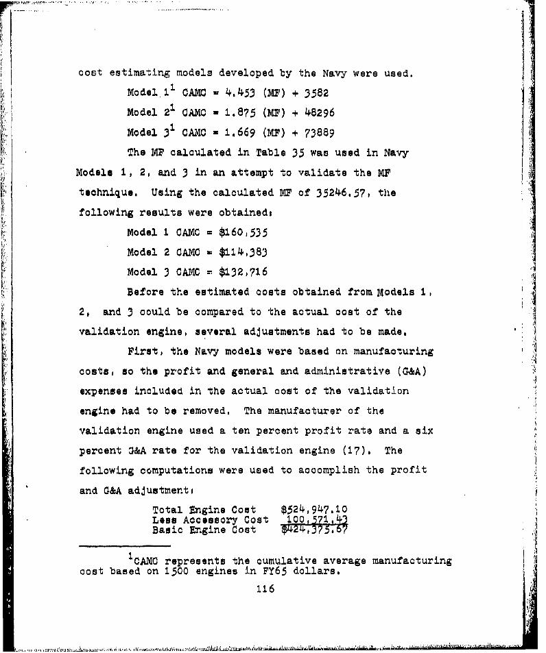
cost estimating models developed by the Navy were used.
Model I OAMC - 4.453 (MF) + 3582
Model 2 CAMC * 1.875 (MV) + 48296
Model 3 CAMC = 1.669 (MF) + 73889
The M? calculated in Table 35 was used in Navy
Models 1, 2, and 3 in an attempt to validate the MF
technique. Using the calculated MF of 35246.57, the
following results were obtained,
Model I CANC m $160,535
Model 2 CAMC = $114,383
Model 3 CAMC = $132,716
Before the estimated costs obtained from Models 1,
2, and 3 could be compared to the actual cost of thevalidation engine, several adjustments had to be made, i
First, the Navy models were based on manufacturing
costs, so the profit and general and administrative (G&A)
expenses included in the actual cost of the validation
engine had to be removed. The manufacturer of the
validation engine used a ten percent profit rate and a six
percent G&A rate for the validation engine (17). The
following computations were used to accomplish the profit J
and G&A adjustmenti
Total Engine Cost $524,947,i0Less Accessory Cost 407,ŽBasic Engine Cost 42T 7 516
1 CAMC represents the cumulative average manufacturingcost based on 1500 engines in FY65 dollars.
116
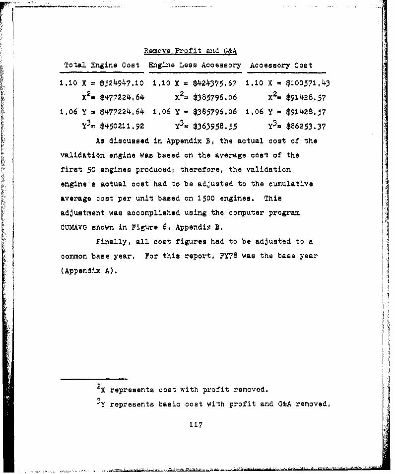
Remove Profit anid G&A
Total Engine Cost Engine Less Accessory Accessory Cost
1.10 x w $52494.7,1o 1.10 X = $424375.67 1.10 X = $100571.43
X2 = $477224,64 X2 = $385796.06 X2 $91428.57
1.06 Y = $477224.64 1.06 Y $385796.06 i.O6 y = $91428.57
y3= $450211.92 Y3 = $363958.55 Y3m $86253.37
As discussed in Appendix B, the actual cost of the
validation engine was based on the average cost of the
first 50 engines producedl therefore, the validation
engine's actual cost had to be adjusted to the cumulative
average cost per unit based on 1500 engines. This
adjustment was accomplished using the computer program
CUMAVG shown in Figure 6, Appendix B.
Finally, all cost figures had to be adjusted to a
common base year. For this report, FY'8 was the base year
(Appendix A).
X represents cost with profit removed,
3Y represents basic cost with profit and G&A removed,
117
APPENDIX D
REGRESSION ANALYSIS
118
I .
The main thrust of the analysis is to evaluate and
measure the dependence of a variable on a set of independent
variables. Within this thesis a dependent variable MP is
regressed on independent variables, such as air flow (AF),
maximum specific fuel consumption (MSFC), and afterburner
(AB). Thus, a meaningful relationship of the dependent
variable to independent variables will hopefully exist,
enabling the prediction of turbine engine cost.
The dependent variable is plotted on the Y axis and
the independent variables are plotted on the X axis, As
depicted in Figure I the regression line is of the form
Y= a + BIX + ei
where
Y = Estimated Maurer Factor
m = the constant added in each case
B = the constant coefficient by which the value ofthe independent variables is multiplied(regression coefficient)
X = the independent variables (turbine engineparameters)
e = the error in prediction, the residual (asdepicted in Figure?)
and is the best fitting line among the data points. The
data points in this analysis are engine parameters and their
associated Maurer Factor.
119
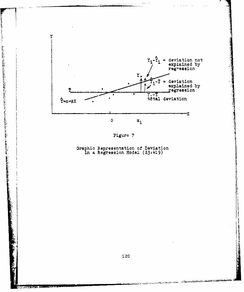
y
=iY deviation notexplained by
=deviation1' ~ explained by
riegress i.on
A t~tal deviation
0 0i
Figure7
Gralhio Representation of~ Deviationn a Regression Model (25,j419)
1.20
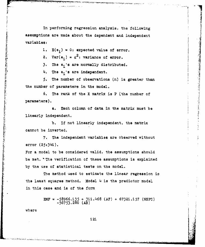
In performing regression analysis, the following
assumptions are made about the dependent and independent
variabless
1. E(ei) = 01 expected value of error.
2. Var(ei) = a2; variance of error.
3. The ei's are normally distributed,
J4, The ej's are independent.
5. The number of observations (n) is greater than
the number of parameters in the model.
6. The rank of the X matrix is P (the number of
parameters).
a, Each column of data in the matrix must be
linearly independent.
b, If not linearly independent, the matrix
cannot be inverted.
7. The independent variables are observed without
error (251341).
For a model to be considered valid, the assumptions should
be met. The verification of these assumptions is explained
by the use of statistical tests on the model.
The method used to estimate the linear regression ia
the least squares method. Model 4 is the predictor model
in this case and is of the form
EMF = -58966.135 + 311.468 (AF) + 67321.157 (MSFC)-56753.280 (AB)
where
121
EPIF = The estimated Maurer Factor
AF ? Air Flow
MSFC = Maximum specific fuel consumption
AB " Afterburner
and to validate the model, the P-test and t-test were
conducted. The predictor model was achieved using a
computer multiple regression subprogram. (See Figure 8 for
the Model 4 statistical program.) This subprogram also
provided the statistics for the F-test and t-test (Table 36).
F-test
An F-test is performed to determine if a statistically
significant relationship exists between the dependent
variable and the independent variables. In Model 4 the F
ratio,
= variance explained by reressionunexplained variance
is equal to 17.98, To determine whether the model is
significant the F ratio is compared to a critical F (Fc)
calculated using an F Statistics Distribution Table
(25,716-717), If F < FC then the null hypothesis (HO)
cannot be rejected.
HO 1 0 02 '" = - 0
However, if F > Fc then Ho can be rejected and further
testing of the model can be continued. In Model 4, F =
17.98 > = 3.32 which is significant, thus reject Ho04
122
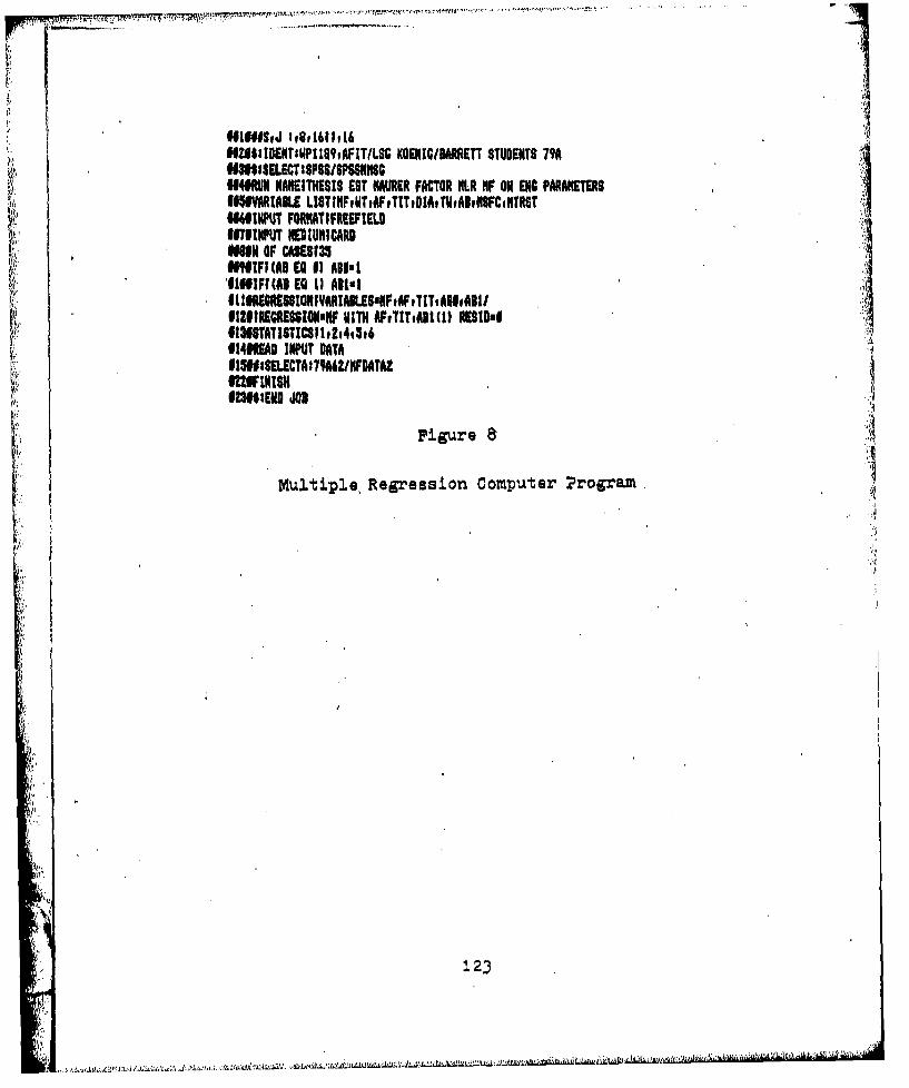
I 71"*IZPI!1DENTINHMPID9AITILS KOENIGIBAtRETT STUDENTS 79A
MORIJN ONAEITHESIS EST NAURER FACTOR MLR HF ON END PARAHETES695PARIAILE LIST INF.UTAFetTIT tDIA.t MAINSFCs NTROTINIMU FORHATIFREEFTELD
IM7IPUT HEDIUNICARD
fr UYf"IF (AD EQ 01 ADM~OfINIFI (AD EQ 11 A8I19
IIZIIPRCRESSIOMaF NITH WTAF, I Me31~ RESI~u*f I3NTATISTlCSIbb24oW,0Z4#00A INPUT DATA915ff SELECTA'79A4/FOATAZ
*Z39SEND Joe
Figure a
Multiple, Regression Compu~ter Program.
123
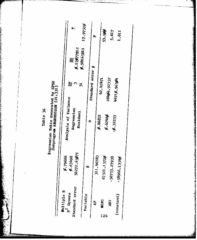
f.4 0.
43.
00
44)
ca% 124
Ak
t tes.
In Model 4 above, the null hypothesis for the overall
Smodel was rejeotedl therefore, at least one of the regressors i
•i ~~(independent variables) in the model was significant., To ii
check the regressor for significance, a t-test was performed
on each of the independent variable's coefficient, the
hypothesis being H0 , 0.
The information was again obtained from Table 36.
The t value associated with each of the independent
variables is equal to the square root of that variable's
F statistic, thusi
tAF 53•9 7.34
t mVr. ZT7 *2. 37
Agan, -VI•" * 1.27
Again, the critical t (to) was taken from the Student's t
Critical Points table (25t713). Since t a 2.042, and t
and tMSFC > t0, air flow and maximum specific fuel
consumption are significant variables in the model.
Afterburner does not prove significant, but the variable
may still add to the model. In Model 4, afterburner was
included (25 0345-346).
Thus far, the F test of the overall model indicated
a good modeli and the t tests of the individual regressors
implied that AF and MSFC were significant regressors.
However, further testing must be accomplished to indicate
whether there exists a relationship among the residuals
125
S... ............................... ... . . .i.. . . • ................ i .. . • ... ...... .... ,.. -......... ... . . ..." - ..- --. -.. . . . .. " -- o
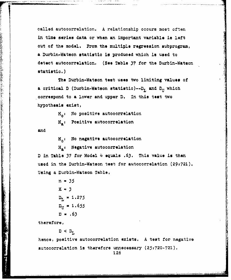
• ,• i• 1• . • - -,s • ,• . •r• . •; • , •, , ,• • _ , 1, • • ; . • : ... . • : •..i,.1..., .....
called autocorrelation. A relationship occurs most often
in time series data or when an important variable is left
out of the model. Prom the multiple regression subprogram,
a Durbin-Watson statistic is produced which is used to
detect autocorrelation, (See Table 37 for the Durbin-Watson
statistic.)
The Durbin-Watson test uses two limiting values of
a critical D (Durbin-Watson statisatio)--DL and DU which
correspond to a lower and upper D. In this test two
hypothesis exist,
H i No positive autocorrelation
Ha, Positive autooorrelation
and
H No negative autocorrelationHgi Negative autooorrelationa
D in Table 37 for Model 4 equals .63. This value is then
used in the Durbin-Watson test for autocorrelation (29,721).
Using a Durbin-Watson Table,
n =35
DL = 1.275
Du - 1.655
D = .63
therefore,
D < DL
hence, positive autocorrelation exists, A test for negative
autocorrelation is therefore unnecessary (251720-721),126
lU
E4)
4J
44
go,
ot
02
4-)0m2
4)
4-2
r)-I
012
.. .. ... ..
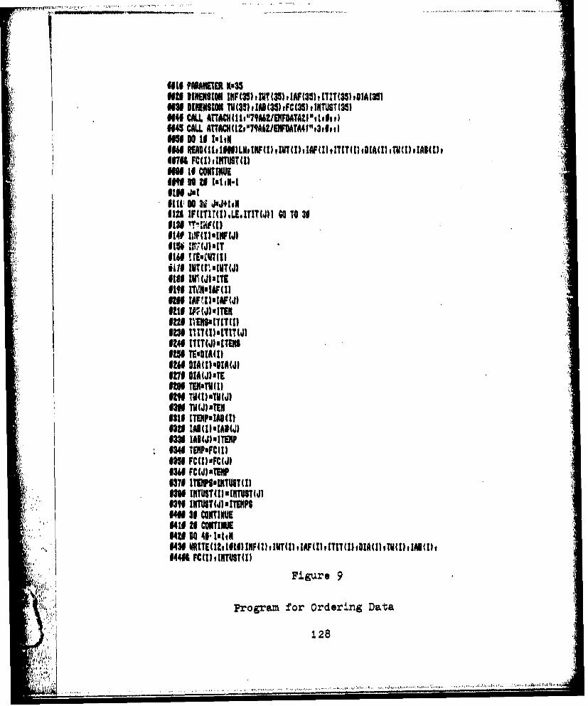
0911 PMARIEIER K1,35IOU3 DINENSION IRF(3) INT(351 IAF(33) ITT(35) #CIA (351MN3 0100NION TV(35) lAO(33 wFC (35), INTUST (33)9649 CALL ATTACH II t1,79A6/ERFlOATA2I,1et #I,M94 CALL ATTACH (Ie"79A62/NFUAA4 V",3s It t
99709 FC1E1hINTUST11)990919 CONTINUEItiIlt" N0 U9 [IeN-1It99 JotIM.;100 W~ JIJMIN1121 IF(ITIT(I.L.E.TITW)) 40 TO 369113 `!i!WK(I)'IFJ
9299 IAFI)'lPW9W1 INT(JoWTTERfill Ir aEYEITI
629ITC~IT(J'IE
329 DIAF1I)'DIA(J1R111 DIAW)'TER
9Z31 t1TU(J)'IYTE9320 IADIT'IAI(J)W$3 MIAI(MIO
V. 934M TENP'VTUIt"9 THCWN(J)
03310 ITERMAI'ITOT0306 INTIMA(3INTSTJ0331 ZINIUTJxI [TERPO
6137 9 CO~aNTNUETl64130 461.1cM[KUSIJ
14406 FC(IhINTUST1Z)
Figure9
Program for Ordering Data
128
S,.~......... . . .. . ...... , ...
The findings of positive autooorrelation in Model 4
indicate that it would not be a reliable predictor of values
for MPs,
129
APPENDIX E
PROFIT ANiD Q&A COST ADJUSTMENT
130
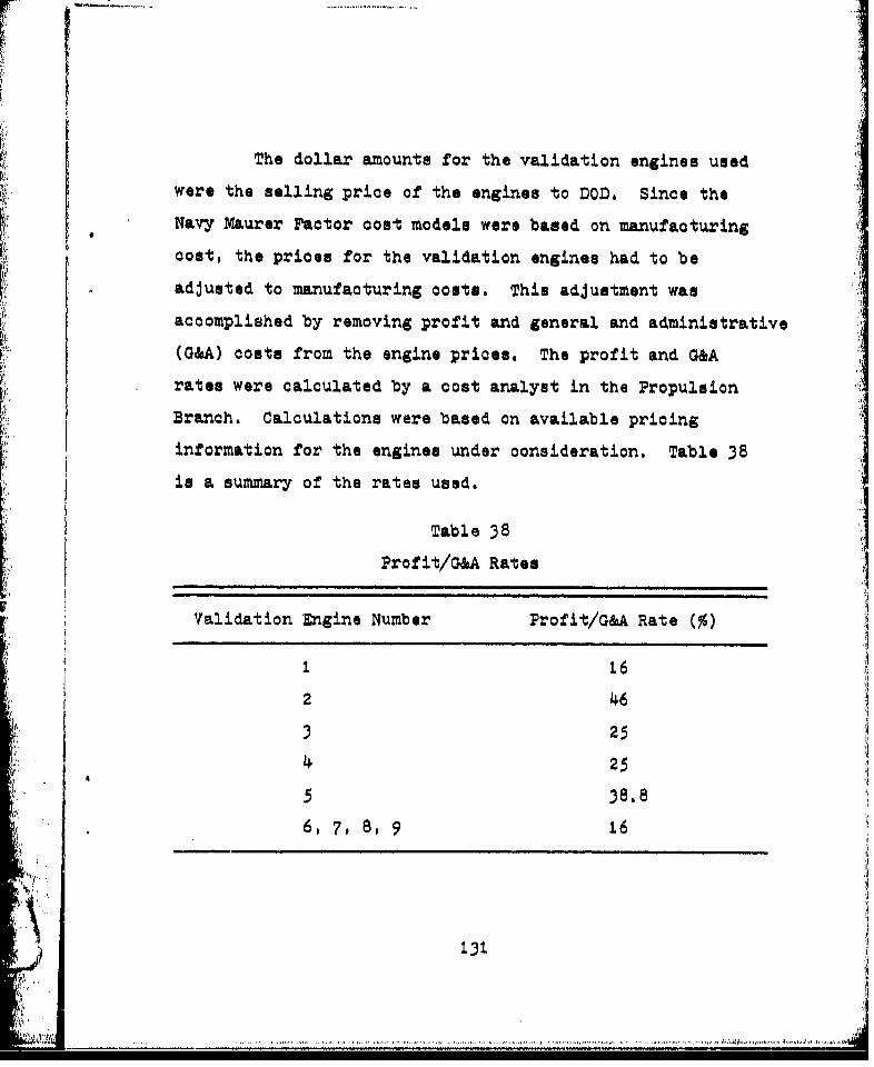
The dollar amounts for the validation engines used
were the selling price of the engines to DOD, Since the
Navy Maurer Factor cost models were based on manufacturing
cost, the prices for the validation engines had to be
adjusted to manufacturing costs. This adjustment was
accomplished by removing profit and general and administrative
(G"A) costs from the engine prices. The profit and G&Arates were calculated by a cost analyst in the Propulsion
Branch. Calculations were based on available pricing
information for the engines under consideration. Table 38
is a summary of the rates used.
Table 38
Prof it/GM Rates
Validation Engine Number Profit/G&A Rate (%)
1. 1.6
2 46
3 25
4 25
5 38.8
* 6, 7, 8, 9 16
131

SELECTED BIBLIOGRAPHY
1.32
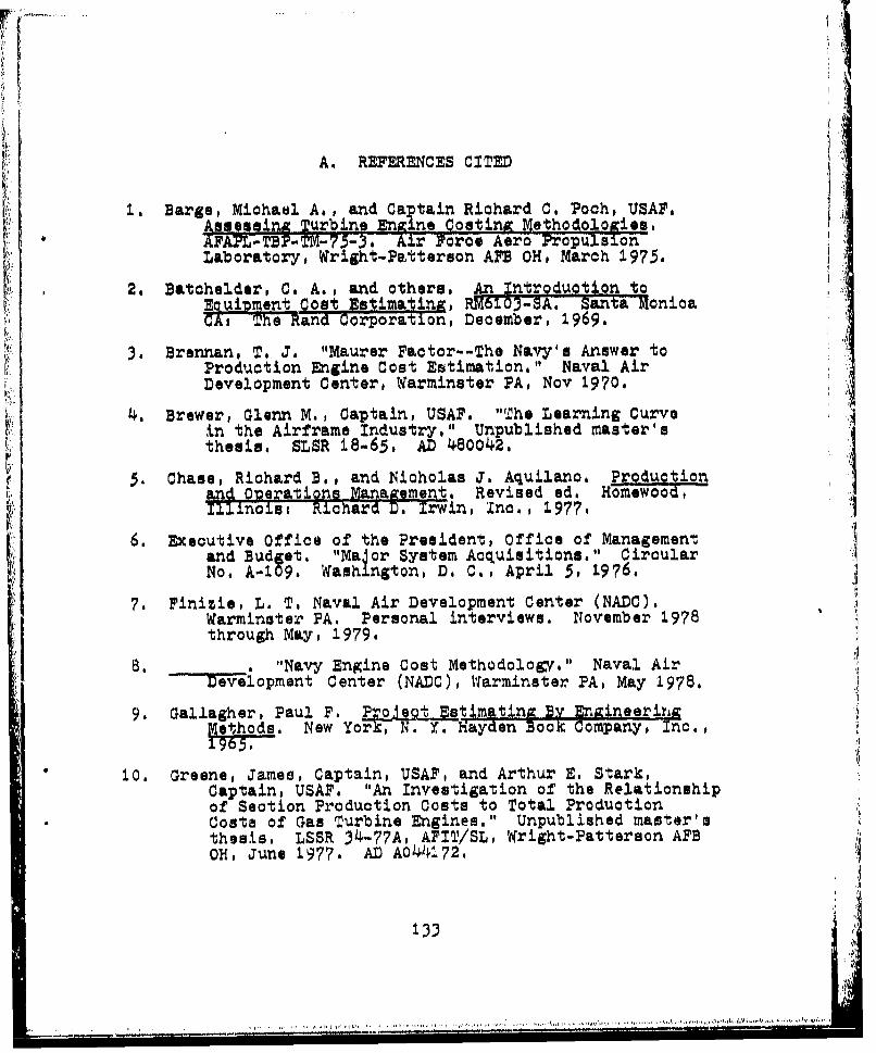
A. REFERENCES CITED
1. Barge, Michael As, and Ca tain Richard C. Pooh, USAF.Fsess-Tng Turbine Engine Costing Methodolocies
AFAYL-TBF-TM-75"3, Air Force Aero PropulsionLaboratory, Wright-Petterson APB OH, March 1975.
2, Batchelder, C. A., and others. An Introduotion toEguipment Cost Estimating, RM6103-SA. Santa MonicaCAs The Rand Corporation, December, 1969,
3. Brennan, T. J. "Maurer Factor--The Navy's Answer toProduction Engine Cost Estimation." Naval AirDevelopment Center, Warminster PA, Nov 1970.
4, Brewer, Glenn M., Captain, USAF. "The Learning Curvein the Airframe Industry," Unpublished master'sthesis. SLSR 18-65, AD 480042.
5. Chase, Richard B., and Nicholas J. Aquilano. Prod otionand Oa rations Management, Revised ed. Homewood,Illinoisi Richard D. irwin, Inc., 1977.
6. Executive Office of the President, Office of Managementand Budge t. "Major System Acquisitions." CircularNo. A-1O99 Washington, D, C., April 5, 1976.
7. Finizie, L. T. Naval Air Development Center (NADC).Warminster PA. Personal interviews. November 1978through May, 1979.
8. , "Navy Engine Cost Methodology." Naval Airx-Dvelopment Center (NADC), Warminster PA, May 1978.
9. Gallagher, Paul F. Prole.o t Estimating By 1npaneerinrgMethods. New YorkI-I. Yr. Hayden Book Company, Inc.,1965.
±0. Greene, James, Captain, USA?, and Arthur E. Stark,Captain, USAF. "An Investigation of the Relationshipof Section Production Costs to Total Production
* Costs of Gas Turbine Engines." Unpublished master'sthesis. LSSR 34-77A, AFIT/SL, Wright-Patterson AFBOH, June 1977. AD A044172.
133
* a n-n
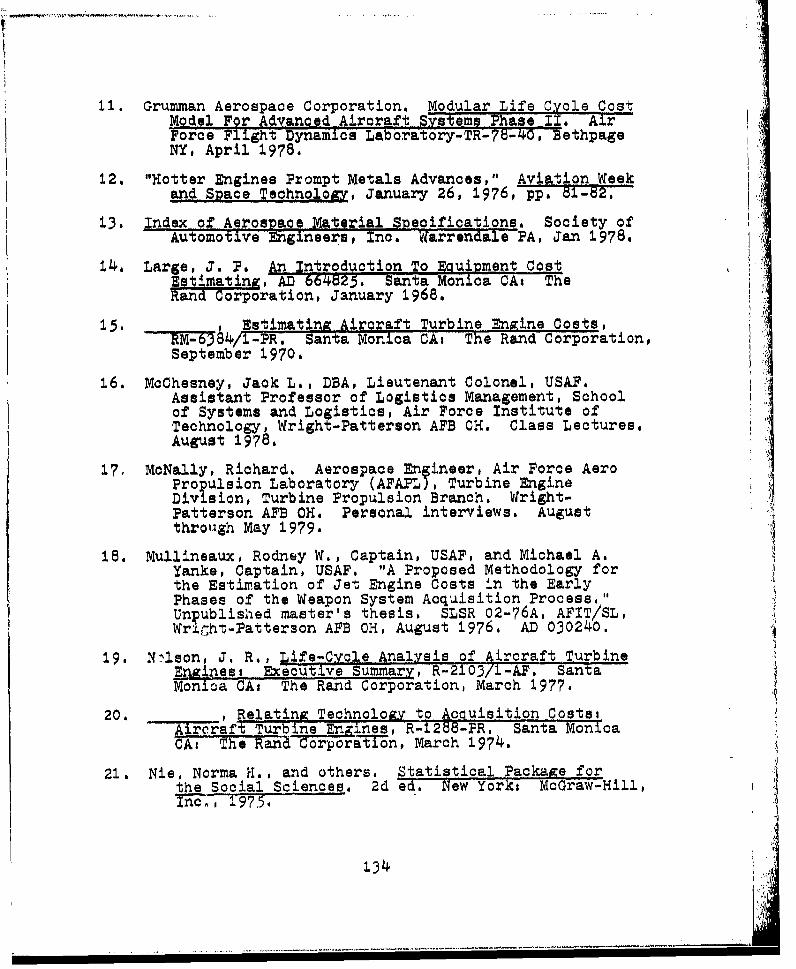
11. Grumman Aerospace Corporation. Modular Life Cycle CostModel For Advanced Aircraft Systems Phase I1. AirForce Flight Dynamics Laboratory-TR-?8-40, BethpageNY, April 1978.
12. "Hotter Engines Prompt Metals Advances," Aviation Weekand Space Technology, January 26, 1976, pp. 81-2.
13. Index of Aerospace Material Specifications. Society ofAutomotive Engineers, Inc. Warrendale PA, Jan 1978,
14, Large, J. P. An 1ntroduction To Eauipment CostEstimating, AD 664825, Santa Monica CA: TheRand Corporation, January 1968.
15. , Estimating Aircraft Turbine Engine Costs,---•84/f-PR. Santa Monica CA: The Rand Corporation,September 1970.
16. McChesney, Jack L., DBA, Lieutenant Colonel, USAF.Assistant Professor of Logistics Management, Schoolof Systems and Logistics, Air Force Institute ofTechnology, Wright-Patterson AFB OH. Class Lectures.August 1978.
17,? McNally, Richard. Aerospace Engineer, Air Force AeroPropulsion Laboratory (AFAPL), Turbine EngineDivision, Turbine Propulsion Branch. Wright-Patterson AFB CH, Personal interviews. August
18. Mullineaux, Rodney W., Captain, USAF, and Michael A.Yanke, Captain, USAF. "A Proposed Methodology forthe Estimation of Jet Engine Costs in the EarlyPhases of the Weapon System Acquisition Process."Unpublished master's thesis. SLSR 02-76A, AFIT/SL,Wright-Patterson AFB OH, August 1976, AD 030240.
19. N'lson, J. R., Life-Cycle Analysis of Airoraft TurbineEnguines: Executive Summary, R-2103/1-AF. SantaMonica CAs The Rand Corporation, March 1977.
20. Relatind Technology to Acquisition Costs, -
" Aircraft Turbine En ines, R-12d-3R. Santa MonicaCAt The Rand'Corporation, March 1974.
21. Nie, Norma H., and others. Statistical Package forthe Social Sciences. 2d id. New Yorks McGraw-Hill,
[ I I I .... I ... i.....I ... I I I I I I I I134I I
22. Pratt-Whitney Aircraft. The Aircraft Gas Turbine Engineandoits Operation. Pratt-Whitney Aircraft,Division of United Technologies, June 1952 (rewrittenMay, 1974).
23. Robinson, Lester L., Beverly A. Zolezzi, and Dean X.Hanink. "Materials Index Factor Methods forEstimating Manufacturing Cost of Advanced PowerPlants." Technical Memorandum, EngineeringOperations, Detroit Diesel Allison, Division ofGeneral Motors Corporation, Indianapolis IN, 1975,
24. Smith, Larry L. Ph D, Lieutenant Colonel, USAF.Associate Professor of Logistics Management, Schoolof Systems and Logistics, Air Force Institute ofTechnology, Wright-Patterson AFB OH. Class Lectures.January through March 1979,
25. U. S. Department of the Air Force. Principles ofContract Pricin , Volume I, Shoo ystems andLogistios, Air Force Institute of Technology (AU),Wright-Patterson AFB OH, June 1975,
26. . Princioles of Contract Pricing, Volume II.School of Systems and Logistics, Air Force Instituteof Technology (AU), Wright-Patterson APB OH, June1975.
27. Watts, A. Frank, Aircraft Turbine Engines-Developmentand Procurement Cost, RM-4670-PE. Santa MonicaCA: The Rand Corporation, November 1965.
28. "Weight, Cost Cuts Spur Composite Work," Aviation Weekand Space Technology., 26 January, 1976_, pp, 73-77.
29. Wonnacott, Thomas H., and Ronald J. Wonnacott,Introductory Statistics for Business and Economics.2d ed. John Wiley and Sons, Inc., 1977.
30. Yamane, Taro. Statistics, An Zntroductory Analysis.2d ed. New Yorks Harper and Row, Publishers, Inc.,1967.
B. RELATED SOURCES
"Inflation Boasts F-15 Program Cost," Aviation Week andSpace Technology, August 2, 1976, pp. 38-39.
135
. ....t......
Lee, Lamar, and Donald W. Dobler. Purchasing and MaterialsManaxemento Xept an•d Cases. 3d ed. New York, McGraw-i:•, Hill Book Companys 1977,
Luettinger, Terry V., Captain, USA?. Life Cycle CostAnalyst, Directorate of Program Control, PropulsionSystem Program Office. Wright-Patterson APB OH. -IPersonal interview. Conducted I Sept 1978.
"1"R & D Costs of JTIO Set at $400 Million," Aviation Weekand SPaoe TechnoloSX, February 2, 1976 p. 3 5,
Taylor, Craig P., Captain, USAF. Chief, Estimating andEvaluation, Directorate of Program Control PropulsionSystem Program Office. Wright-Patterson AFB OH.Personal interview. Conducted I Sept 1978.
"Titanium Industry Banks on Use in B-1I," Aviation Week andSpace Technoloon, January 26, 1.976, pp. 73-77,
U, S. Air Force Systems Command. "Turbine Engine LifeCycle Cost Model." ASD/YZ office, Wright-PattersonAPB OH, I February 1977.
136
ABBREVIATIONS AND ACRONYMS
143
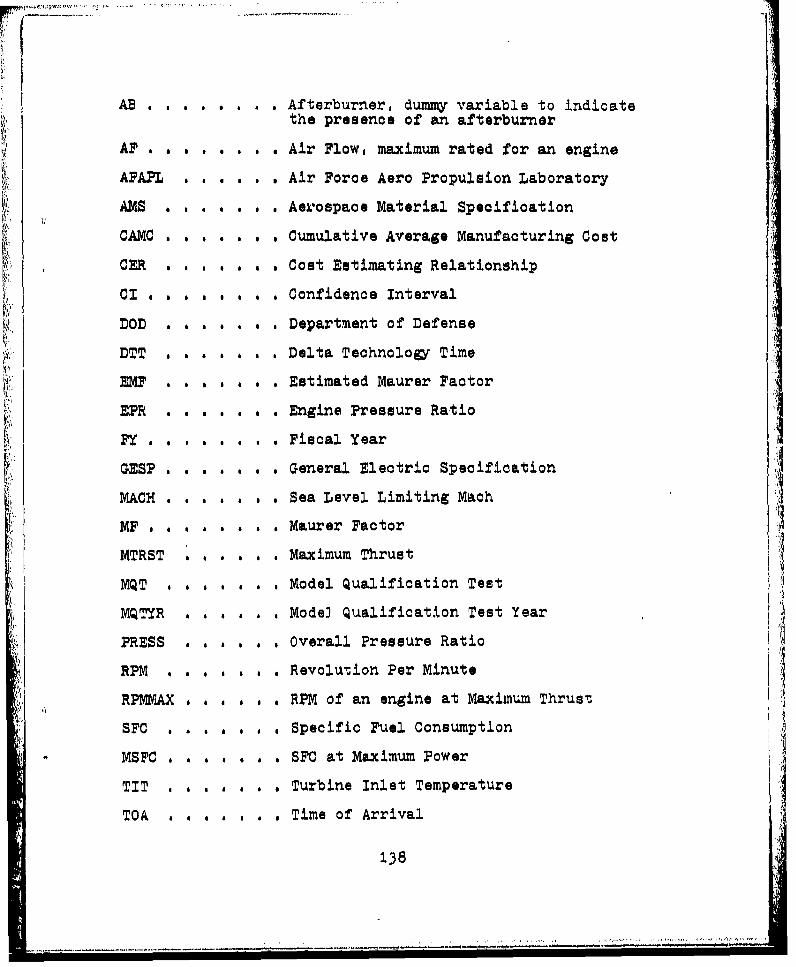
AB . . . . . . . . Afterburner, dummy variable to indicatethe presence of an afterburner
A? . . . . . . . . Air Flow, maximum rated for an engine
AFAPL . . . . . . Air Force Aero Propulsion Laboratory
AMS a , * 4 , * * Aerospace Material Specification
CAMC . . . . . . . Cumulative Average Manufacturing Cost
CER . . . . . . . Cost Estimating Relationship
CI . . . . . . . . Confidence Interval
DOD . . . . . . . Department of Defense
DTT . . . . . . . Delta Technology Time
EMF . . . . . . . Estimated Maurer Factor
EPR . a * . . . Engine Pressure Ratio
FY . .. . Fiscal Year
GESP . . . . . . . General Electric Specification
MACH ....... Sea Level Limiting Mach
MFP. ..... .Maurer Factor
MTRST . . a . a . Maximum Thrust
MQT , .... a Model Qualification Test
MQTYR . . . . . . Model Qualification Test Year
PRESS . . . . . . Overall Pressure Ratio
RPM a a . a a a Revolution Per Minute
RPMMAX . . a . a . RPM of an engine at Maximum Thrust
SFC . . . . . . . Specific Fuel Consumption
MSFC . . . . . . . SFC at Maximum Power
TIT . . . . . . . Turbine Inlet Temperature
TOA . . . . . . . Time of Arrival
138