Chronicle of a War Foretold: The MacroeconomicEffects of Anticipated Defense Spending Shocks ∗

Nadav Ben Zeev† Evi Pappa‡

October 14, 2014

Abstract

We identify US defense news shocks as shocks that best explain future movementsin defense spending over a five-year horizon and are orthogonal to current defensespending. Our identified shocks are strongly correlated with the Ramey (2011) newsshocks, but explain a larger share of macroeconomic fluctuations and have significantdemand effects. Fiscal news induces significant and persistent increases in output,consumption, investment, hours and the interest rate. Standard DSGE models failto produce such a pattern. We propose a sticky price model with variable capitalutilization, capital adjustment costs, and rule-of-thumb consumers that replicates theempirical findings and allows us to test the validity of our methodology for extractinganticipated fiscal shocks from the data.

JEL classification: E62, E65, H30

Key words: SVAR, maximum forecast error variance, defense news shocks, DSGE model

∗We are grateful to Markus Bruckner, Fabio Canova, Efrem Castelnuovo, Sandra Eickmeier, Wouter DenHaan, Luca Dedola, Maren Froemel, Nir Jaimovich, Karel Mertens, Anton Nakov, Tomasso Oliviero, PaoloSurico, Valerie Ramey, Nora Traum, and participants at the VIII REDg Workshop, CSEF seminar, the 18thT2M Annual Conference, the Budensbank Seminar, the 2014 ESSIM Meeting, and the 18th Conference onMacroeconomic Analysis for helpful comments and suggestions.†Ben Gurion University of the Negev, Israel. E-mail: nadavbz@bgu.ac.il.‡European University Institute, UAB, BGSE, and CEPR. E-mail: evi.pappa@eui.eu.

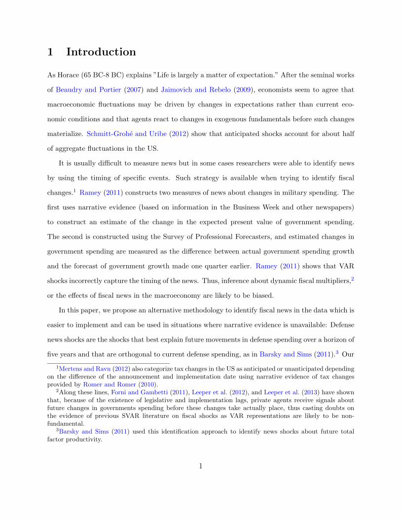
1 Introduction

As Horace (65 BC-8 BC) explains ”Life is largely a matter of expectation.” After the seminal works

of Beaudry and Portier (2007) and Jaimovich and Rebelo (2009), economists seem to agree that

macroeconomic fluctuations may be driven by changes in expectations rather than current eco-

nomic conditions and that agents react to changes in exogenous fundamentals before such changes

materialize. Schmitt-Grohe and Uribe (2012) show that anticipated shocks account for about half

of aggregate fluctuations in the US.

It is usually difficult to measure news but in some cases researchers were able to identify news

by using the timing of specific events. Such strategy is available when trying to identify fiscal

changes.1 Ramey (2011) constructs two measures of news about changes in military spending. The

first uses narrative evidence (based on information in the Business Week and other newspapers)

to construct an estimate of the change in the expected present value of government spending.

The second is constructed using the Survey of Professional Forecasters, and estimated changes in

government spending are measured as the difference between actual government spending growth

and the forecast of government growth made one quarter earlier. Ramey (2011) shows that VAR

shocks incorrectly capture the timing of the news. Thus, inference about dynamic fiscal multipliers,2

or the effects of fiscal news in the macroeconomy are likely to be biased.

In this paper, we propose an alternative methodology to identify fiscal news in the data which is

easier to implement and can be used in situations where narrative evidence is unavailable: Defense

news shocks are the shocks that best explain future movements in defense spending over a horizon of

five years and that are orthogonal to current defense spending, as in Barsky and Sims (2011).3 Our

1Mertens and Ravn (2012) also categorize tax changes in the US as anticipated or unanticipated dependingon the difference of the announcement and implementation date using narrative evidence of tax changesprovided by Romer and Romer (2010).

2Along these lines, Forni and Gambetti (2011), Leeper et al. (2012), and Leeper et al. (2013) have shownthat, because of the existence of legislative and implementation lags, private agents receive signals aboutfuture changes in governments spending before these changes take actually place, thus casting doubts onthe evidence of previous SVAR literature on fiscal shocks as VAR representations are likely to be non-fundamental.

3Barsky and Sims (2011) used this identification approach to identify news shocks about future totalfactor productivity.

1

identified defense news shocks are strongly correlated with the Ramey (2011) news shocks, but they

explain a much larger fraction of the variability in all real variables at business cycle frequencies.

Also, they have a significant and more positive effect in the economy. In particular, anticipated

fiscal shocks induce a significant and persistent increase in output, consumption, investment, hours

and the interest rate. Hence, the component of the shock identified using the maximum forecast

error variance methodology (henceforth MFEV) that is independent of the Ramey shock series

contains important information on future defense spending. We illustrate further this point by

showing that the Ramey news series is missing important information about fiscal news in the

beginning of the 1950s, the end of 1970s and the mid 1990s.

Standard models are incapable of generating significant demand effects from defense spending

news. In fact, in these models consumption falls after a news shock and output reacts less strongly.

We have augmented a standard New Keynesian DSGE model with (a) variable capital utilization

and capital adjustment costs and (b) rule of thumb consumers in order to generate theoretical

responses to fiscal news that match the data. We use the model to simulate data and employ our

proposed identification scheme in the simulated data to estimate the theoretical impulse responses

and show that our proposed methodology recovers accurately the true shocks.

Several other studies analyze the macroeconomic effects of anticipated government spending

shocks. Mertens and Ravn (2010), for example, use a DSGE model to derive a fiscal SVAR estimator

that is applicable when shocks are permanent and anticipated and use it with US data. Our

framework is less restrictive since it can deal with temporary fiscal shocks and uses medium-

run rather than long-run constraints to identify them. Leeper et al. (2012) identify two types of

fiscal news concerning government spending and tax policies. They identify government spending

news using the Survey of Professional Forecasters and map the reduced-form estimates of news

into a DSGE framework. They find that fiscal news is a time-varying process and incorrectly

assuming time-invariant processes to model news might be misleading. Gambetti (2012) assesses

the information content of government spending news constructed as the difference between the

forecast of government spending growth over the next three quarters made by the agents at time t

2

(measured with the Survey of Professional Forecasters) and the forecast of the same variable made

at time t − 1. He finds that the identified government spending news shock in a VAR generates

Keynesian type of effects, increasing output and consumption and real wages before the actual

increase in spending but crowding out private investment.

The remainder of the paper is organized as follows. Section 2 describes the econometric frame-

work. Section 3 presents the main empirical results and in section 4 we examine their sensitivity

to changes in the model specification. In Section 5 we present the theoretical model and in Sec-

tion 6 we report results from testing our empirical methodology on simulated data and Section 7

concludes.

2 Econometric Strategy

2.1 Data

The data covers the period from 1947:Q1 to 2008:Q4. Recent work by Leeper et al. (2013) and

Ramey (2011) has discussed the issue of missing information with respect to defense news events

and how it can undermine identification in SVAR’s. One efficient way to address this problem

is by directly adding more information to the VAR, as in Sims (2012) and Forni and Gambetti

(2011). Thus, together with real per capita defense spending, we also include in the VAR the

Ramey (2011) measure of defense news shocks.4 Apart from enabling us to alleviate the missing

information problem, the inclusion of this series allows us to check how the news series we extract

correlates with the latter series and to compare the effects of our shock with the effects of Ramey’s

news shock.

In addition to the defense spending variable and the Ramey (2011) news series, we also include

in the VAR output, hours, consumption , and investment, all in real per capita terms, as well as

the real manufacturing wage, the Barro and Redlick (2011) average marginal tax rate, the interest

4This the narrative-based series Ramey constructed from newspaper archives.

3

rate on 3 month T-bills, and CPI inflation. The data comes from Ramey’s website.5

2.2 Identifying Defense News Shocks

The defense news shock is identified as the shock that best explains future movements in defense

spending over a horizon of five years and that is orthogonal to current defense spending. To

obtain such shock we need to find the linear combination of VAR innovations contemporaneously

uncorrelated with current defense spending which maximally contributes to defense spending’s

future forecast error variance as in Barsky and Sims (2011). The orthogonality restriction relative

to defense spending is important since it requires the identified shock to have no contemporaneous

effect on defense spending.

Let yt be a kx1 vector of observables of length T . Let the reduced form moving average

representation in the levels of the observables be:

yt = B(L)ut (1)

where B(L) is a kxk matrix polynomial in the lag operator, L, and ut is the kx1 vector of reduced-

form innovations. We assume that reduced-form innovations and structural shocks, εt, are linked

by

ut = Aεt (2)

Equations (1) and (2) imply

yt = C(L)εt (3)

where C(L) = B(L)A and εt = A−1ut. The matrix A must satisfy AA′ = Σ, where Σ is the

variance-covariance matrix of reduced-form innovations. There are, however, an infinite number of

5http://weber.ucsd.edu/ vramey/

4

A′s that satisfy the restriction. For some arbitrary orthogonalization, A (for example, the Choleski

decomposition), the space of permissible impact matrices can be written as AD, where D is a k x

k orthonormal matrix (D′ = D−1, which entails D′D = DD′ = I).

The h step ahead forecast error is

yt+h − Etyt+h =

h∑τ=0

Bτ ADεt+h−τ (4)

where Bτ is the matrix of moving average coefficients at horizon τ . The contribution to the forecast

error variance of variable i attributable to structural shock j at horizon h is

Ωi,j =h∑τ=0

Bi,τ Aγγ′A′B′i,τ (5)

where γ is the jth column of D, Aγ is a kx1 vector corresponding with the jth column of a possible

orthogonalization, and Bi,τ represents the ith row of the matrix of moving average coefficients at

horizon τ . We put defense spending in the first position in the system, and index the defense

news shock as 1. Our identification procedure requires finding the γ which maximizes the sum of

contributions to the forecast error variance of defense spending from horizon 0 to horizon H (the

truncation horizon), subject to the restriction that these shocks have no contemporaneous effect

on defense spending. Formally, we need to solve the following optimization problem

γ∗ = argmaxγ

H∑h=0

Ω1,1(h) =

H∑h=0

h∑τ=0

B1,τ Aγγ′A′B′1,τ (6)

subject to A(1, j) = 0 ∀j > 1 (7)

γ(1, 1) = 0 (8)

γ′γ = 1 (9)

The first two constraints impose on the identified news shock to have no contemporaneous effect

on defense spending. The third restriction ensures that γ is a column vector belonging to an

orthonormal matrix. This normalization implies that the identified shocks have unit variance.

5

In the benchmark set up H=20 quarters. Hence, the defense news shock we identify is the shock

that is orthogonal to defense spending and which maximally explains future variation in defense

spending over a horizon of five years. The lag of the model is set to 4 which is a midway between

what standard criteria suggest (The Akaike criteria favors six lags, the Hannan-Quinn information

and Schwartz criteria favor two lags, and the likelihood ratio test statistic chooses eight lags). We

examine the robustness of our results to alternative lag lengths and alternative H in Section 4.

3 Empirical Evidence

3.1 Impulse Responses

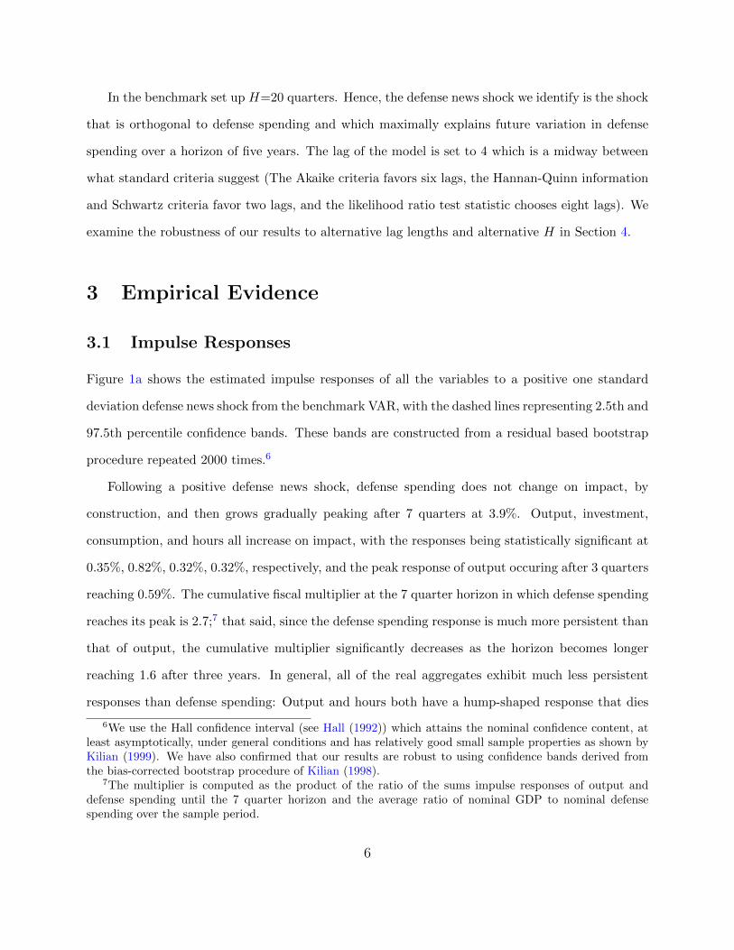
Figure 1a shows the estimated impulse responses of all the variables to a positive one standard

deviation defense news shock from the benchmark VAR, with the dashed lines representing 2.5th and

97.5th percentile confidence bands. These bands are constructed from a residual based bootstrap

procedure repeated 2000 times.6

Following a positive defense news shock, defense spending does not change on impact, by

construction, and then grows gradually peaking after 7 quarters at 3.9%. Output, investment,

consumption, and hours all increase on impact, with the responses being statistically significant at

0.35%, 0.82%, 0.32%, 0.32%, respectively, and the peak response of output occuring after 3 quarters

reaching 0.59%. The cumulative fiscal multiplier at the 7 quarter horizon in which defense spending

reaches its peak is 2.7;7 that said, since the defense spending response is much more persistent than

that of output, the cumulative multiplier significantly decreases as the horizon becomes longer

reaching 1.6 after three years. In general, all of the real aggregates exhibit much less persistent

responses than defense spending: Output and hours both have a hump-shaped response that dies

6We use the Hall confidence interval (see Hall (1992)) which attains the nominal confidence content, atleast asymptotically, under general conditions and has relatively good small sample properties as shown byKilian (1999). We have also confirmed that our results are robust to using confidence bands derived fromthe bias-corrected bootstrap procedure of Kilian (1998).

7The multiplier is computed as the product of the ratio of the sums impulse responses of output anddefense spending until the 7 quarter horizon and the average ratio of nominal GDP to nominal defensespending over the sample period.

6

off after three years; consumption and investment responses return to zero after a year and a half.

It is also apparent that the real wage declines significantly following the news shock. Given

that the real wage is measured as the product wage in the manufacturing sector rather than the

consumption wage, this result can be interpreted along the lines of Ramey and Shapiro (1998) who

showed that the relative price of manufactured goods rises significantly during a defense buildup

and, thus, product wages in these industries can fall at the same time that the consumption wage

is unchanged or rising. The news shock also raises the average marginal income tax rate, inflation

and interest rates. Note that the tax rate increases in a gradual manner reflecting the notion that

defense news shocks foretell future increases in both defense spending and tax rates.

Figure 1b shows the estimated impulse responses to a positive one standard deviation shock to

the Ramey news variable. Two important differences stand out. First, our identified news shock

has a larger effect on defense spending: the peak response of spending following the Ramey news

shock is 3.3% compared to 3.9% following our news shock. Second, the responses of all the macro

variables are significantly weaker. For example, the peak response of output occurs after 5 quarters,

generating a multiplier of 1.13. On the other hand, the responses of hours are insignificant at all

horizons. Furthermore, the responses of investment, consumption, and interest rates, though not

significant, have signs which are the opposite of those obtained with our news series.

3.2 Forecast Error Variance Decomposition

Figure 2 shows the share of the forecast error variance of the endogenous variables attributable

to our defense news shocks and the Ramey news shock. In general, our news shock explains a

larger share of the forecast error variance of all variables. For example, it explains 54% of the

variation in defense spending at the three year horizon compared to 38% for the Ramey news

shock. Moreover, our news shock explains 70% of the variation in the Ramey news variable on

impact. This indicates that our identified news shock is strongly related to Ramey’s news shock

though it appears to contain more information about future defense spending.

In addition to the defense spending variable, our MFEV news shock accounts for a much larger

7

share of the forecast error variance of all other variables: It explains 23% and 28% of output and

hours variation at the one year horizon, respectively, compared to 2% and 0% explained by Ramey’s

news shock; and a much bigger share of the variation in the nominal variables and the Barro and

Redlick (2011) average marginal tax rate. In particular, our news shocks explains 21% of the

variation in inflation at the three quarter horizon and 22% of the variation in the tax rate at the

two year horizon, compared to 9% and 4% of the Ramey news shock, respectively. Furthermore,

our news shock explains 13% of the variation in interest rates at the two year horizon, compared

to zero in the case of Ramey’s news shock.

To examine whether the differences between the contributions of the MFEV news shock and

the Ramey news shock to the variables’ variation are statistically significant, we estimated for all

variables the p-value for the null hypothesis that the difference between the contribution the MFEV

news shock and the Ramey news does not exceed zero. Each estimated p-value was obtained as the

proportion of bootstrap values of the contribution difference of the two shocks not exceeding zero.8

Our estimated p-values indicate that the differences are generally significant. Table 1 presents these

results. To be concise, we focus on the horizon for which the point estimate of the contribution

difference is maximal. P-values are sufficiently low for most variables: The contribution differences

for defense spending, output, hours, the Barro and Redlick (2011) average marginal tax rate,

and investment appear to be highly significant with p-values of 0%, 2.2%, 1.1%, 3.2%, and 6.1%,

respectively, and those corresponding to inflation and consumption are moderately significant with

p-values of 10.6% and 12.5%, respectively. The zero p-value for the null hypothesis that the

difference between the contribution of our news shock and the Ramey news shock to the defense

spending variation is not positive strongly indicates that our news shock contains relatively more

information about future defense spending.

8As noted in Lutkepohl (2005) on p. 712, this estimation procedure will yield p-value estimates that areconsistent under general assumptions.

8

3.3 The Additional Information Content in the MFEV News Shock

Series

The results presented thus far have established that there is valuable information contained in our

MFEV news series that is absent from the narrative-based Ramey (2011) shock series.9 To further

illustrate the important difference between the two shocks, we run an exercise in which we projected

our MFEV shock series onto the shock to the Ramey (2011) news series and collected the residual,

and then projected all of the other variables in the VAR onto their own lags and the current and

lagged values of the residual from the first step and estimated the impulse responses of the variables

to the residual.10

The first step residual (henceforth MFEVORT) is shown in Figure 3, along with shaded areas

that represent the dates at which the Ramey series is uninformative, i.e., contains zeroes. It

is apparent that the mid-1990s deficit reducing Clinton era and the Obama election period are

captured by very large negative realizations of our shock that are not accounted for by Ramey’s

narrative-based approach. Furthermore, there are various other large shocks that our identification

method captures but are not accounted for by the narrative approach, e.g., the very large late 1952

shock (third largest overall) which can be associated with the Eisenhower election; the very large

shock at the end of 1980 (second largest overall) when Reagan got elected; and the largest shock

of the series that took place in the second quarter of 1978 and can be associated with the Saur

Revolution which signified the onset of communism in Afghanistan and preluded the 1979 Soviet

war in Afghanistan.

The impulse responses to MFEVORT are shown in Figure 4: MFEVORT has a significant effect

on future defense spending as well as on all real and nominal variables. More specifically, it raises the

9It is worth noting that this result holds despite the strong correlation between the two series on 0.85.That is, the component of the MFEV series that is unrelated to the Ramey news shock, albeit small relativeto the shared component, seems to contain valuable information.

10We thank Karel Mertens for suggesting us this exercise. We excluded Ramey’s series from the estimationundertaken in the second step so as to avoid collinearity resulting from the fact that the first step residualis a linear combination of all lagged variables. Since the first step residual is orthogonal by construction toRamey’s series, thus, rendering the inclusion of Ramey’s series redundant, we proceeded with the secondstep estimation without the Ramey series.

9

real aggregates, inflation, interest rates, and taxes, and starts to have a significant effect on defense

spending after six quarters. The peak effect on defense spending is also economically significant at

nearly 2%, indicating that there is additional information about future defense spending beyond

that contained in the narrative-based series of Ramey. Taken together, the results of this section

suggest that while the narrative approach is informative, it can only capture part of the news

present in the data and is therefore inferior to our MFEV identification method which can do a

better job of picking the vast information content available in the data.

4 Robustness

This section addresses six potentially important issues regarding the analysis undertaken in the

previous section. The first is the concern that assuming different lag specifications or alternative

truncation horizons for the MFEV optimization problem may produce different results. The second

issue pertains to the potential effect that altering the sample period, such that either the World War

II period is included or the Korean War period is excluded, may have on the benchmark results.

The third issue we examine is whether our shock is correlated with the identified defense shock of

Fisher and Peters (2011) which corresponds to the innovation to the accumulated excess returns

of large US military contractors. The fourth issue we address is whether our results are robust

to excluding the Ramey (2011) news series from the VAR, which is important to confirm given

that narrative-based defense news measures are generally unavailable for most countries. The fifth

robustness check pertains to the specification of a linear time trend in the benchmark VAR. Finally,

we confirm that our results are not driven by a positive correlation of our identified shock with

other structural disturbances that are identified in the literature as potential drivers of business

cycle fluctuations.11

11We have also tried a battery of sensitivity tests regarding the number of variables in the VAR and theirordering: Our results are insensitive to such changes and we do not present them here for economy of space.

10

4.1 VAR Lags and the Truncation Horizon

Figure 5a shows the impulse responses obtained with lag lengths, from 3 to 6. As evident, the

impulse responses to all of the variables are in general similar both qualitatively and quantitatively.

The only noticeable difference is in the response of the Barro and Redlick (2011) income tax rate

which is weaker and negative on impact for the model with 6 lags. Figure 5b displays the responses

for four separate horizons, H = 10, 20 (benchmark), 30, and 40. The results are similar for all

horizons.

4.2 Changing the Sample

Figures 6a and 6b correspond to Figures 1a and 1b with the only difference being that now the

VAR is estimated using the larger sample period of 1939:Q2-2008:Q4. Including the World War II

period introduces additional large fiscal events that are relatively much larger in magnitude (See

also Ramey (2011)).

It is apparent that, by and large, the results are qualitatively unchanged for both news shocks,

with the exception of the responses of investment which falls after our news shock in the extended

sample. While the point estimate impact effect on investment is still positive, investment starts to

decline much sooner as compared to the benchmark sample though the decline becomes significant

only after 6 quarters.

Quantitatively responses are stronger than in the previous section and the MFEV news shock

still generates much stronger responses than the Ramey news shock. The peak effects on output

and hours are twice as large as before and the peak response of defense spending is 5.7% following

our news shock compared to 2.9% following the Ramey news shock. These differences are most

likely related to the very large fiscal news events that took place in the World War II period and

are seen to have a noticeable effect on the responses of output and hours.

Perotti (2007) argues that the Korean War was unusually large and it should be excluded from

the analysis of the effects of government spending. Figures 7a and 7b present responses estimated

using the smaller sample period of 1955:Q1-2008:Q4. The results are unchanged: our news shock

11

continues to generate significant demand effects that are stronger than the Ramey news shock

effects.

4.3 Relation of News Shocks to the Fisher and Peters (2011) De-

fense Shock Series

Fisher and Peters (2011) have recently identified government spending shocks as the innovations

to the accumulated excess returns of large US military contractors. Figures 8a and 8b plot the

responses of the economy to a news shocks identified with our and Ramey’s approach, when the

VAR includes the Fisher and Peters (2011) excess return series.

The main results are robust to adding the excess return series to the VAR. Yet, an interesting

result emerges with respect to the added excess returns variable. While our news shock significantly

increases the excess returns of large defense contractors, the Ramey news shock has an insignificant

effect on this variable. Thus, our methodology might recover shocks which contain more information

about future fiscal policy relative to the Ramey news series.

4.4 Excluding the Ramey (2011) News Series

Given that narrative-based news shock measures are often unavailable for most countries, it is

important to alleviate the concern that our empirical results are driven by our inclusion of the

Ramey (2011) news series and that the applicability of our method is limited to economies for

which such measures are available. To this end, we applied our methodology to a VAR that

excludes the Ramey (2011) news series. The results of this exercise are presented in Figure 9. It is

apparent that the main results remain qualitatively unchanged: the identified news shock continues

to raise the real aggregates, inflation, interest rates, and taxes, with defense spending following a

delayed and gradual rise after the news shock realizes.

Note that although defense spending responds less strongly to the identified news shocks when

the Ramey (2011) series is absent from the VAR,12 the responses of the other variables are generally

12The contribution of the shock to the variation in defense spending (not shown here) after three years is

12

stronger than the benchmark ones. Furthermore, the correlation between the identified MFEV news

shock with the corresponding benchmark shocks obtained from the VAR that includes the Ramey

(2011) series is 0.58, a strong correlation though clearly one that manifests a non-negligible wedge

between the two identified shock series. In sum, while it is clear that including the Ramey (2011)

series increases the importance of the shock in explaining the future variation in defense spending

and thus improves identification, it is still evident that a significant effect on defense spending is

identified along with a significant effect on the other important macroeconomic variables also when

the Ramey (2011) series is excluded.

4.5 Adding a Linear Trend to the VAR

Given that various authors have chosen to add a linear trend to VARs with fiscal shocks (e.g.,

Blanchard and Perotti (2002), Ramey (2011), and Mertens and Ravn (2012)), in this section we

present results from estimating a VAR in which a linear trend was added. Figure 10 presents the

impulse responses from this robustness exercise: it is clear that the results are unchanged, both

qualitatively and quantitatively, with the MFEV news shock continuing to have significant demand

effects.

4.6 Relation of MFEV News Shock to Other Structural Distur-

bances

An additional concern that may arise from the benchmark results is that the identified MFEV news

shock is correlated with other structural disturbances. To address this concern, we computed the

correlation between the identified MFEV news shock and up to four lags and leads of the Romer

and Romer (2004) monetary policy shock measure, Romer and Romer (2010) tax shock measure,

shock to the real price of oil, the TFP news shock from Barsky and Sims (2011), the innovation

to the U.S. economic policy uncertainty index of Baker et al. (2012), and the unanticipated and

16% after three years compared to 54% in the benchmark case.

13

anticipated tax shocks constructed by Mertens and Ravn (2012).13 Apart from the Barsky and Sims

(2011) TFP news shock series which was used in its raw form, all other shocks were constructed as

the residuals of univariate regressions of each of the six raw shock measures on four own lags.

In Figure 11 we plot contemporaneous and lead and lag correlations between the MFEV news

shocks and the other five shocks we consider, together with the corresponding 95% asymptotic

confidence intervals. The results indicate that the cross-correlations are small and insignificant,

with all correlations being lower than 19% in absolute value. Thus, the fact that our shock is well

identified and it has significant effects on output, consumption, investment, and hours relative to

Ramey’s news cannot be driven by mixing disturbances when using our identification approach. .

4.7 Relation of MFEVORT to Other Structural Disturbances

Given that MFEVORT, i.e., the component of our identified defense news shocks that is orthogonal

to the the shock to the Ramey (2011) news series, is an important driver behind this paper’s results,

it is important to show that it too is not correlated with the macroeconomic shocks considered

in the previous section. Figure 12 presents the same output as Figure 11 only that the cross-

correlations are now computed for the MFEVORT series. It is apparent that MFEVORT is generally

uncorrelated with all leads and lags of the considered shocks: the correlations are small and largely

statistically insignificant, all being lower than 18% in absolute terms. That MFEVORT is not

correlated with monetary policy shocks is especially important given the strong effect it was found

to have on interest rates.

Nevertheless, there are two marginally significant correlations worth noting and addressing: i)

a correlation of 17% between one lag of the Mertens and Ravn (2012) anticipated tax shock and

MFEVORT and ii) a contemporaneous correlation of -18% between the Barsky and Sims (2011)

TFP news shock and our identified defense news shock. While these correlations are low, we still

13The Mertens and Ravn (2012) anticipated tax shock is effectively available in the form of 17 separateseries, each corresponding to a different anticipation horizon at which the news shock took place. Wetransform these series into a single summary news shock measure by adding the various series thus producinga single series of tax news shocks, albeit with heterogenous anticipation horizons. The results of both thissection and the next section are unaffected by taking instead the separate series themselves.

14

view it as important to conduct two supplementary robustness exercise so as to ensure that our

results are not driven by these two other news shocks. First, we added the Mertens and Ravn

(2012) raw anticipated tax measure to the model of Section 3.3 as an endogenous variable.14.

Second, we projected the utilization-adjusted TFP measure of Fernald (2012) upon current and

lagged MFEVORT.15 The motivation for conducting the first exercise is that obtaining similar

results for MFEVORT when controlling for the lagged values of tax news shocks would ensure that

this paper’s results are not driven by anticipated tax shocks; the motivation for doing the second

exercise is that directly and formally testing the effect of MFEVORT on TFP at future horizons

would allow to asses to what extent, if any, MFEVORT is linked to TFP news shocks.

Figures 13 and 14 present the impulse responses from the tax news augmented model of the

first exercise and the response of TFP to MFEVORT from the second exercise, respectively. We

can clearly see that controlling for lagged tax news shocks has essentially no effect on the impulse

responses of MFEVORT, which continues to have significant demand effects raising the real ag-

gregates as well as inflation and interest rates. Also note that the effects of MFEVORT on the

anticipated tax measure are both statistically and economically insignificant at all horizons. Turn-

ing to the TFP response, it is strongly indicated that MFEVORT shock has no significant effect on

TFP at all horizons; note also that the negative point estimate, in addition to being statistically

insignificant, is also not economically significant having a peak response of less than 0.17% after

one year and hovering at less than 0.13% for nearly all horizons. Importantly, the result of the

second exercise not only removes the concern that our findings are driven by TFP news shocks but

it also eliminates the worry that unanticipated TFP shocks, which are the more conventional TFP

shock traditionally considered in macroeconomic models, play a role in driving this paper’s results.

Taken together, the results from all three robustness exercises of this section suggest that we

can be fairly confident that our findings are not driven by other structural shocks. Moreover, the

main takeaway from the results of this section is that MFEVORT does in fact represent added

14The tax news augmented model was estimated with a sample period ending in the first quarter of 2006(the ending date of the Mertens and Ravn (2012) raw anticipated tax measure).

15This regression was estimated with the sample period for which MFEVORT is available, i.e., 1948:Q1-2008:Q4.

15

information contained in our MFEV news shock series relative to the Ramey shock series. This is

highly encouraging as it is this added information that effectively produces the stronger results for

the MFEV news shock.16

5 Anticipated Defense Spending Shocks in a DSGE

Model

It is easy to show that a standard flexible, or sticky price DSGE model cannot replicate the empiri-

cal impulse responses with respect to defense news shocks. Both models fail to match qualitatively

and quantitatively the responses present in the data. For standard DSGE models, even under

the assumption of sticky prices, consumption reacts negatively in the impact period of the antic-

ipated shock and the responses of the real variables fall short of the empirical impulse responses

quantitatively.

Clearly, many mechanisms having been proposed for inducing positive responses of consumption

after government spending shocks and for propagating news shocks in DSGE models in the litera-

ture. Various theoretical models have been suggested for generating increases in consumption after

a fiscal expansion. These mechanisms include: (a) consumption and hours’ complementarity in the

utility function (see Monacelli and Perotti (2008), Hall (2009), Christiano et al. (2011) and Naka-

mura and Steinsson (2011)); (b) a lax monetary policy (see Canova and Pappa (2011), Christiano

et al. (2011) and Erceg and Linde (2013)); (c) rule-of-thumb consumers (see Gali et al. (2007)); (d)

deep habits (see Mertens and Ravn (2012)); (e) spending reversals (see Muller et al. (2009)) and

(g) home production (see Gnocchi (2013)). On the other hand, the ‘News Driven Business Cycles’

literature has focused on the problem of generating intuitive news driven business cycles. Several

16We have also confirmed a positive connection between MFEVORT and revisions of expectations aboutfederal spending from the Survey of Professional Forecasters (SPF). More specifically, we have constructedthe revision of expectations made at period t of growth in federal spending from period t to period t + 3;we then projected this SPF-based news variable on current and lagged values of MFEVORT and found astatistically significant impact response of 0.13%. These results are available upon request from the authors.

16

modifications of the standard model have been suggested for propagating TFP news shocks:17 (a)

making consumption or leisure an inferior good (see, Eusepi and Preston (2009)); (b) using wealth

in the utility function (Karnizova (2012)); (c) allowing for sticky prices and accommodative mone-

tary policy (see Christiano et al. (2010), Khan and Tsoukalas (2012), Blanchard et al. (2009) among

others) ; (d) adopting a multi-sector structure (see, Beaudry and Portier (2007)); (e) introducing

investment adjustment costs and variable capital utilization (see Jaimovich and Rebelo (2009)) and

(f) introducing search and matching frictions (see, Den Haan and Kaltenbrunner (2009)).

We have played with combinations of the different suggested mechanism in order to be able to

replicate the empirical findings. We introduce two modifications to the standard sticky price model

in order to bring its predictions closer to the data: (a) introducing variable capacity utilization in

the production function as in Jaimovich and Rebelo (2009);18 and (b) introducing rule of thumb

consumers, assuming that 33% of the population does not have access to capital markets and simply

consumes its disposable income. Next we present briefly the model and describe the theoretical

responses to fiscal news shocks.

5.1 A Theoretical Model

The economy is inhabited by two types of households, optimizers and rule of thumb consumers.

The problem of the optimizers is given below.

Optimizing Households

There is a share 1 − λ of optimizers that derive utility from private consumption, Cot and leisure,

1 − Not . At time 0 they choose sequences for consumption, labor supply, capital to be used next

period Kt+1, nominal state-contingent bonds, Dt+1 and government bonds, Bt+1 to maximize their

17Beaudry and Portier (2013) provide an extensive literature review on the topic.18Following Burnside and Eichenbaum (1996) we assume that production depends on effective utilized

capital and that capital depreciation depends negatively of the capital utilization rate.

17

expected discounted utility:

E0

∞∑t=0

βtu(Cot , Not ) = E0

∞∑t=0

βt[Cot (1−No

t )1−φ]1−σ − 1

1− σ(10)

where 0 < β < 1, and σ > 0. Here β is the subjective discount factor and σ a risk aversion

parameter. Available time each period is normalized at unity. The financially unconstrained

household maximizes utility subject to the sequence of budget constraints:

Pt(Cot + It) + EtQt,t+1Dt+1+R−1t Bt+1 ≤ (11)

(1− τ lt )PtwtNot + [rt − τk(rt − δ(Ut))]PtKt +Dt +Bt + Ξt

where (1−τ lt )PtwtNot , is the after tax nominal labor income, [rt−τk(rt−δ(Ut))]PtKt is the after tax

nominal capital income (allowing for depreciation), Ξt, are nominal profits from the firms (which

are owned by consumers), and Tt are lump-sum taxes.

We assume complete private financial markets: Dt+1 is the holdings of the state-contingent

nominal bond that pays one unit of currency in period t + 1 if a specified state is realized and

Qt,t+1 is the period-t price of such bonds, and Rt the gross return of a government bond Bt.

Private capital accumulates according to:

Kt+1 = It + (1− δ(Ut))Kt − ν(Kt+1

Kt

)Kt (12)

Following Burnside and Eichenbaum (1996), we assume that production depends on effective uti-

lized capital and that capital depreciation depends positively on the capital utilization rate:

δ (Ut) = ψUφt (13)

where ψ,φ > 0. The parameter φ in equation (13) determines the effect of utilization on the

rate of depreciation of capital. When φ > 0 , ∂δ∂U > 0, whereas when φ = 0, capital utilization does

not affect the rate at which capital depreciates.

18

and the function ν is parameterized as:

ν

(Kt+1

Kt

)=b

2

[Kt+1 − (1− δ)Kt

Kt− δ(1)

]2(14)

where b determines the size of the adjustment costs. Since optimizers own and supply capital to

the firms, they bear the adjustment costs.

Financially constrained households

The remaining fraction of households, λ, are financially constrained. Rule-of-thumb households

fully consume their current labor income. They cannot smooth their consumption in the face of

fluctuations in labor income and intertemporally substitute in response to changes in interest rates.

Their period utility is the of the same form as for optimizers and its given by (10). And their

budget constrained is given by:

PtCrt = (1− τ lt )PtwtN r

t (15)

Aggregation

Aggregate consumption and hours are given by a weighted average of the corresponding variables

for each consumer type. That is,

Ct = (1− λ)Cot + λCrt (16)

and

Nt = (1− λ)Not + λN r

t (17)

Firms

Firm j produces output according to:

Yt(j) = (ZtNt(j))1−α(Ut(j)Kt(j))

α (18)

19

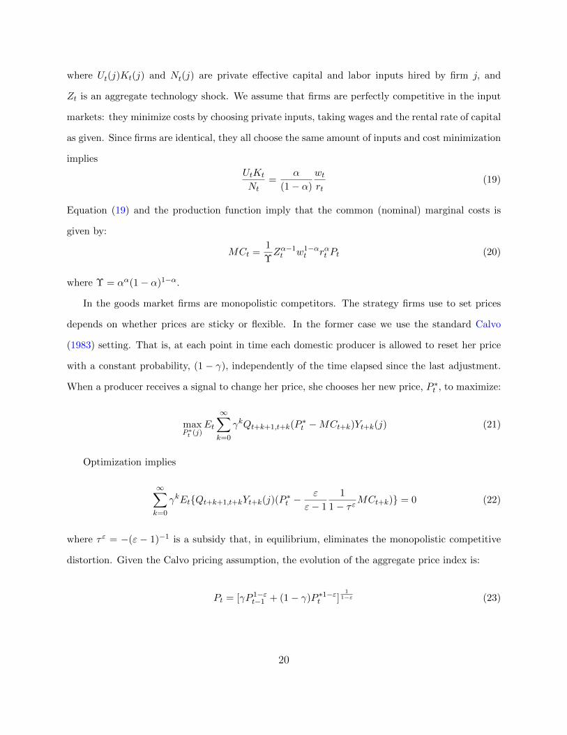
where Ut(j)Kt(j) and Nt(j) are private effective capital and labor inputs hired by firm j, and

Zt is an aggregate technology shock. We assume that firms are perfectly competitive in the input

markets: they minimize costs by choosing private inputs, taking wages and the rental rate of capital

as given. Since firms are identical, they all choose the same amount of inputs and cost minimization

implies

UtKt

Nt=

α

(1− α)

wtrt

(19)

Equation (19) and the production function imply that the common (nominal) marginal costs is

given by:

MCt =1

ΥZα−1t w1−α

t rαt Pt (20)

where Υ = αα(1− α)1−α.

In the goods market firms are monopolistic competitors. The strategy firms use to set prices

depends on whether prices are sticky or flexible. In the former case we use the standard Calvo

(1983) setting. That is, at each point in time each domestic producer is allowed to reset her price

with a constant probability, (1 − γ), independently of the time elapsed since the last adjustment.

When a producer receives a signal to change her price, she chooses her new price, P ∗t , to maximize:

maxP ∗t (j)

Et

∞∑k=0

γkQt+k+1,t+k(P∗t −MCt+k)Yt+k(j) (21)

Optimization implies

∞∑k=0

γkEtQt+k+1,t+kYt+k(j)(P∗t −

ε

ε− 1

1

1− τ εMCt+k) = 0 (22)

where τ ε = −(ε − 1)−1 is a subsidy that, in equilibrium, eliminates the monopolistic competitive

distortion. Given the Calvo pricing assumption, the evolution of the aggregate price index is:

Pt = [γP 1−εt−1 + (1− γ)P ∗1−εt ]

11−ε (23)

20

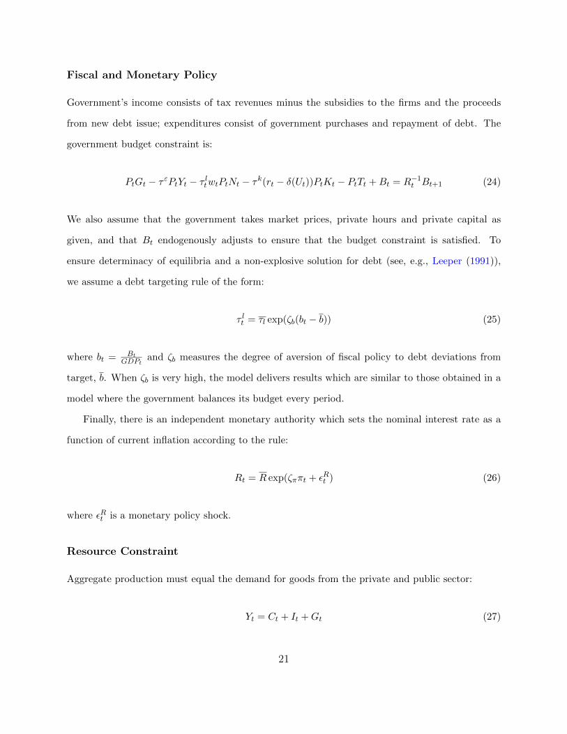
Fiscal and Monetary Policy

Government’s income consists of tax revenues minus the subsidies to the firms and the proceeds

from new debt issue; expenditures consist of government purchases and repayment of debt. The

government budget constraint is:

PtGt − τ εPtYt − τ ltwtPtNt − τk(rt − δ(Ut))PtKt − PtTt +Bt = R−1t Bt+1 (24)

We also assume that the government takes market prices, private hours and private capital as

given, and that Bt endogenously adjusts to ensure that the budget constraint is satisfied. To

ensure determinacy of equilibria and a non-explosive solution for debt (see, e.g., Leeper (1991)),

we assume a debt targeting rule of the form:

τ lt = τl exp(ζb(bt − b)) (25)

where bt = BtGDPt

and ζb measures the degree of aversion of fiscal policy to debt deviations from

target, b. When ζb is very high, the model delivers results which are similar to those obtained in a

model where the government balances its budget every period.

Finally, there is an independent monetary authority which sets the nominal interest rate as a

function of current inflation according to the rule:

Rt = R exp(ζππt + εRt ) (26)

where εRt is a monetary policy shock.

Resource Constraint

Aggregate production must equal the demand for goods from the private and public sector:

Yt = Ct + It +Gt (27)

21

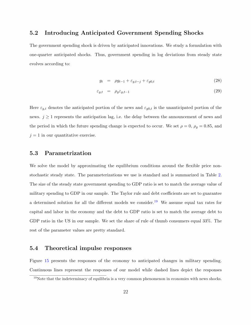
5.2 Introducing Anticipated Government Spending Shocks

The government spending shock is driven by anticipated innovations. We study a formulation with

one-quarter anticipated shocks. Thus, government spending in log deviations from steady state

evolves according to:

gt = ρgt−1 + εg,t−j + εg0,t (28)

εg,t = ρgεg,t−1 (29)

Here εg,t denotes the anticipated portion of the news and εg0,t is the unanticipated portion of the

news. j ≥ 1 represents the anticipation lag, i.e. the delay between the announcement of news and

the period in which the future spending change is expected to occur. We set ρ = 0, ρg = 0.85, and

j = 1 in our quantitative exercise.

5.3 Parametrization

We solve the model by approximating the equilibrium conditions around the flexible price non-

stochastic steady state. The parameterizations we use is standard and is summarized in Table 2.

The size of the steady state government spending to GDP ratio is set to match the average value of

military spending to GDP in our sample. The Taylor rule and debt coefficients are set to guarantee

a determined solution for all the different models we consider.19 We assume equal tax rates for

capital and labor in the economy and the debt to GDP ratio is set to match the average debt to

GDP ratio in the US in our sample. We set the share of rule of thumb consumers equal 33%. The

rest of the parameter values are pretty standard.

5.4 Theoretical impulse responses

Figure 15 presents the responses of the economy to anticipated changes in military spending.

Continuous lines represent the responses of our model while dashed lines depict the responses

19Note that the indeterminacy of equilibria is a very common phenomenon in economies with news shocks.

22

of the standard sticky price model (NK model) and dotted lines the responses of a standard DSGE

model with flexible prices (RBC model) to the shock.20 Our proposed model captures well the

dynamics with respect to fiscal news. It matches the empirical response of consumption whereas

the other two standard models fail to do so and it generates significant responses to fiscal news

relative to the standard RBC model. Relative to the standard NK model, the responses of the

modified economy to the anticipated shock are more persistent. Output, consumption and labor

increase for more than a year after the news. Investment declines at a slower pace relative to

the standard NK model, while the real wage is not reacting much initially and increases with a

delay. Finally, the nominal interest and inflation (not shown in the picture since its responses are

proportional to the responses of the nominal rate) increase persistently after the shock. Thus, apart

from the responses of the real wage, the model captures reasonably well the dynamics of the real

variables in response to fiscal news.21 Given that the responses of the real wage in the data changed

with the sample, we prefer not to change the model specification in order to change this result.

5.4.1 Discussion of the propagation mechanism and alternatives

In this subsection we investigate the importance of the different assumptions we have incorporated

in the model for the transmission of fiscal news shocks. We start by investigating whether the

nominal part of the model is necessary for our analysis. The first column of Figure 16 presents

responses when we assume flexible prices in our benchmark economy. As it is apparent, real

responses under flexible prices are weak due to the absence of the demand effect that propagates

the effects of the fiscal news in the economy by increasing labor demand and real wages and, hence,

the consumption of rule of thumbs and consequently aggregate consumption.

In order to obtain increases in private consumption after fiscal news we have introduced a share

of financially constrained consumers in the model economy. Alternatively, we could have assumed

20In the NK and RBC models utilization does not vary in response to the shocks and the rule of thumbconsumers share is set to zero.

21In simulations that we do not present here for economy of space we show that the model is consistentwith the responses to other shocks such as contemporaneous and news TFP shocks and contemporaneousand news investment specific shocks and monetary policy shocks.

23

complementarities between consumption and leisure by adopting the preference specification in

Jaimovich and Rebelo (2009). We perform this exercise in the second column of Figure 16. All

real variables react to the shock with the same sign as in our benchmark specification, apart

from the real wage that is now falling after a fiscal news shock and the nominal interest rate

that is counterfactually falling. Responses for this model are quantitative smaller for the adopted

calibration, but the major drawback for using this model is that it does not fit the responses of the

economy to a monetary policy shock and for that reason we have decided to use the model with

rule of thumb consumers as our benchmark.

Turning to rule of thumb consumers, the behavior of those households is, by definition, insulated

from movements in real interest rates. Moreover, since these agents consume their disposable income

and since in the presence of sticky prices, their income is increased through the increases in the

real wage induced by the increased labor demand and the increase in tax revenues when the shock

arrives, those agents will increase consumption after the fiscal news shock. As the third column

of Figure 16 shows the presence of financially constrained individuals guarantees an increase in

consumption on impact after the shock, and propagates the effects of fiscal news in the economy.

Also variable capital utilization and adjustment costs are important for generating persistence

responses to fiscal news, as seen in the first column of Figure 17. In the absence of variable capital

utilization and capital adjustment costs, firms miss an additional margin to react to the increased

demand generated by the expected shock and are constrained to increase more labor demand. This

results in higher increases in wages which translates into higher increases in consumption by rule

of thumb consumers. At the same time, investment is crowded out by the increase in private

consumption and increases by a smaller amount relative to the benchmark model. Overall, the

demand effects of the shock become even stronger. Yet, the responses to the shock of all variables

are much less persistent.

5.4.2 Other Assumptions that Help Propagate Fiscal News Shocks

Evans and Karras (1998) estimate private consumption and military spending to be complements

24

and at the same time estimate the share of financially constrained individuals to be 30% in the

US. We investigate how the assumption of financially constrained individuals coupled with comple-

mentarity of military spending and private consumption affect the dynamics of the model economy

by introducing military spending directly in the utility function. The responses of the modified

economy are presented in the second column of Figure 17. Assuming complementarity between mil-

itary and private spending enhances the propagation mechanism of anticipated shocks and helps

the model fit better the data.

Finally, many authors have shown (see, e.g., Canova and Pappa (2011)) that the interaction

between fiscal and monetary policy is crucial for the propagation of fiscal shocks. In the third

column of Figure 17 we plot responses of the model economy when we assume a lower coefficient

for the Taylor rule in (26) - setting ζπ = 1. A laxer monetary policy does indeed allow for stronger

demand effects from fiscal news shocks.

6 A Test of our Methodology

In this section we test our methodology through the lens of our model. To this end, we simulate

series from our model and use our identification strategy in these series in order to see whether

we can recover the true shocks. In particular, we simulate 2000 sets of data with 248 observations

each using as the data generating process the model of Section 5.1. For each simulation, we

apply our identification method on the artificial data and include in the Monte Carlo VAR the

same variables that we used in the empirical exercise.22 The two structural shocks in the model

are the unanticipated and anticipated defense spending shocks, which we draw from the normal

distribution. To avoid singularity, we attach eight measurement errors to all variables in the model

apart from defense spending, all of which are also drawn from normal distributions. The standard

22The only difference from the empirical VAR is that we do not include a narrative-based news measurebecause our theoretical model does not contain a natural counterpart to the Ramey (2011) news series.Nevertheless, we have confirmed that the simulation results are generally insensitive to adding a variablethat is equal to the true news shock series and some reasonably calibrated measurement error that couldproxy for the Ramey news.

25

deviations of the two defense shocks and the measurement errors are presented in Table 3.

Figure 18 depicts both the theoretical and estimated impulse responses averaged over the sim-

ulations to a defense news shock. The theoretical responses are represented by the solid lines and

the average estimated responses over the simulations are depicted by the dashed lines, with the

dotted lines depicting the 2.5th and 97.5th percentiles of the distribution of estimated impulse

responses. It is apparent that the estimated empirical impulse responses are generally unbiased

and capture the dynamics of the variables following the news shock quite well. The unbiasedness

of the estimated responses of the variables coupled with the observation that the lower bands of

the confidence intervals are significantly above zero are very encouraging.

Table 4 reports the average correlation between the identified defense news shock and the true

defense news shock across simulations, along with 95% confidence interval bands. The average

correlation between the identified defense news shock and the true defense news shock across sim-

ulations is 0.84. Moreover, 2.5th and 97.5h percentile correlations are 0.78 and 0.88, respectively.

Taken together, the results of this section demonstrate that our identification method is suitable

for identifying defense spending news shocks.

7 Conclusion

We show that news about military spending do affect significantly aggregate demand and explain

a significant fraction of output fluctuations. In contrast with Ramey (2011), fiscal news generate

significant Keynesian type of effects in the economy, increasing persistently output, consumption,

investment, hours, the interest rate and inflation.

We propose a DSGE model that can explain some of the facts we have revealed and use it to

test our methodology. Our empirical strategy for identifying fiscal news shocks passes the test in

simulated data. We are able to show that identifying fiscal news shocks as shocks that explain

future movements in defense spending over a five-year horizon and that are orthogonal to current

spending in simulated data recovers the true fiscal news shocks.

26

Our results are useful to both academics and policymakers. First, we propose a new methodol-

ogy for the identification of news about fiscal policy changes. It is objective and does not require

the readings of newspapers sources and, as a result, can be applied for countries with weak or no

newspaper archives. Second, we have shown that our approach captures better information about

future military spending increases relative to Ramey (2011) approach. Third, we show that the

presence of rigidities and financially constrained individuals are key assumptions for matching the

empirical findings. Financial frictions matter for aggregate fluctuations, even when the latter are

induced by news shocks. Finally, according to our estimates, news about future changes in military

spending account for a non-negligible share of output fluctuations at business cycle frequencies.

Since anticipation effects are estimated to be significant and economically important, policymakers

should be cautious in announcing policy changes that can affect agents’ expectations about future

government spending. Or reversing this argument, policymakers can use policy announcements as

a tool for responding to the cycle when constrained by budgetary or other types of restrictions.

27

References

Baker, S. R., Bloom, N. and Davis, S. J.: 2012, Policy uncertainty: a new indicator, CentrePiece -

The Magazine for Economic Performance 362, Centre for Economic Performance, LSE.

Barro, R. and Redlick, C.: 2011, Macroeconomic effects from government purchases and taxes, The

Quarterly Journal of Economics 126(1), 51–102.

Barsky, R. and Sims, E. R.: 2011, News shocks and business cycles, Journal of Monetary Economics

58(3), 235–249.

Beaudry, P. and Portier, F.: 2007, When can changes in expectations cause business cycle fluctua-

tions in neo-classical settings?, Journal of Economic Theory 135(1), 458 – 477.

Beaudry, P. and Portier, F.: 2013, News driven business cycles: Insights and challenges, Working

Paper 19411, National Bureau of Economic Research.

Blanchard, O. J., L’Huillier, J.-P. and Lorenzoni, G.: 2009, News, noise, and fluctuations: An

empirical exploration, NBER Working Papers 15015, National Bureau of Economic Research,

Inc.

Blanchard, O. and Perotti, R.: 2002, An empirical characterization of the dynamic effects of changes

in government spending and taxes on output, The Quarterly Journal of Economics 117(4), 1329–

1368.

Burnside, C. and Eichenbaum, M.: 1996, Factor-hoarding and the propagation of business-cycle

shocks, American Economic Review 86(5), 1154–1174.

Calvo, G. A.: 1983, Staggered prices in a utility-maximizing framework, Journal of Monetary

Economics 12(3), 383–398.

Canova, F. and Pappa, E.: 2011, Fiscal policy, pricing frictions and monetary accommodation,

Economic Policy 26(68), 555–598.

28

Christiano, L., Eichenbaum, M. and Rebelo, S.: 2011, When is the government spending multiplier

large?, Journal of Political Economy 119(1), 78–121.

Christiano, L., Ilut, C. L., Motto, R. and Rostagno, M.: 2010, Monetary policy and stock market

booms, NBER Working Papers 16402, National Bureau of Economic Research, Inc.

Den Haan, W. J. and Kaltenbrunner, G.: 2009, Anticipated growth and business cycles in matching

models, Journal of Monetary Economics 56(3), 309–327.

Erceg, C. J. and Linde, J.: 2013, Is there a fiscal free lunch in a liquidity trap?, Journal of the

European Economic Association (forthcoming) .

Eusepi, S. and Preston, B.: 2009, Labor supply heterogeneity and macroeconomic co-movement,

NBER Working Papers 15561, National Bureau of Economic Research, Inc.

Evans, P. and Karras, G.: 1998, Liquidity constraints and the substitutability between private and

government consumption: The role of military and non-military spending, Economic Inquiry

36(2), 203–14.

Fernald, J.: 2012, A quarterly utilization-adjusted series on total factor productivity, Technical

report, Federal Reserve Bank of San Francisco.

Fisher, J. D. M. and Peters, R.: 2011, Using stock returns to identify government spending shocks,

Economic Journal 120(544), 414–436.

Forni, M. and Gambetti, L.: 2011, Fiscal foresight and the effects of government spending,

Manuscript, Universitat Autonoma de Barcelona.

Gali, J., Lopez-Salido, J. D. and Valles, J.: 2007, Understanding the effects of government spending

on consumption, Journal of the European Economic Association 5(1), 227–270.

Gambetti, L.: 2012, Government spending news and shocks, Working paper, Universitat Autonoma

de Barcelona.

29

Gnocchi, S.: 2013, Monetary commitment and fiscal discretion: The optimal policy mix, American

Economic Journal: Macroeconomics 5(2), 187–216.

Hall, P.: 1992, The Bootstrap and Edgeworth Expansion, Springer-Verlag.

Hall, R. E.: 2009, By how much does gdp rise if the government buys more output?, Brookings

Papers on Economic Activity 40(2 (Fall)), 183–249.

Jaimovich, N. and Rebelo, S.: 2009, Can news about the future drive the business cycle?, American

Economic Review 99(4), 1097–1118.

Karnizova, L.: 2012, News shocks, productivity and the U.S. investment boom-bust cycle, The

B.E. Journal of Macroeconomics 12(1), 15.

Khan, H. and Tsoukalas, J.: 2012, The quantitative importance of news shocks in estimated DSGE

models, Journal of Money, Credit and Banking (forthcoming) .

Kilian, L.: 1998, small sample condence intervals for impulse response function, The Review of

Economics and Statistics 80(2), 218–230.

Kilian, L.: 1999, Finite-sample properties of percentile and percentile-t bootstrap confidence inter-

vals for impulse responses, The Review of Economics and Statistics 81(4), 652–660.

Leeper, E. M.: 1991, Equilibria under ’active’ and ’passive’ monetary and fiscal policies, Journal

of Monetary Economics 27(1), 129–147.

Leeper, E. M., Richter, A. W. and Walker, T. B.: 2012, Quantitative effects of fiscal foresight,

American Economic Journal: Economic Policy 4(2), 115–44.

Leeper, E. M., Walker, T. B. and Yang, S. S.: 2013, Fiscal foresight and information flows, Econo-

metrica 81(3), 1115–1145.

Lutkepohl, H.: 2005, New introduction to multiple time series analysis, Springer.

30

Mertens, K. and Ravn, M. O.: 2010, Measuring the impact of fiscal policy in the face of anticipation:

A structural VAR approach, The Economic Journal 120(544), 393–413.

Mertens, K. and Ravn, M. O.: 2012, Empirical evidence on the aggregate effects of anticipated and

unanticipated us tax policy shocks, American Economic Journal: Economic Policy 4(2), 145–81.

Monacelli, T. and Perotti, R.: 2008, Fiscal policy, wealth effects, and markups, NBER Working

Papers 14584, National Bureau of Economic Research, Inc.

Muller, G., Corsetti, G. and Meier, A.: 2009, Fiscal stimulus with spending reversals, IMF Working

Papers 09/106, International Monetary Fund.

Nakamura, E. and Steinsson, J.: 2011, Fiscal stimulus in a monetary union: Evidence from u.s.

regions, NBER Working Papers 17391, National Bureau of Economic Research, Inc.

Perotti, R.: 2007, In search of the transmission mechanism of fiscal policy, NBER Working Papers

13143, National Bureau of Economic Research, Inc.

Ramey, V. A.: 2011, Identifying government spending shocks: It’s all in the timing, The Quarterly

Journal of Economics 126(1), 1–50.

Ramey, V. A. and Shapiro, M. D.: 1998, Costly capital reallocation and the effects of government

spending, Carnegie-Rochester Conference Series on Public Policy 48(1), 145–194.

Romer, C. and Romer, D.: 2004, A new measure of monetary shocks: Derivation and implications,

American Economic Review 94(4), 1055–1084.

Romer, C. and Romer, D.: 2010, The macroeconomic effects of tax changes: Estimates based on a

new measure of fiscal shocks, American Economic Review 100(3), 763–801.

Schmitt-Grohe, S. and Uribe, M.: 2012, What’s news in business cycle?, Econometrica (forthcom-

ing) .

31

Sims, E. R.: 2012, News, non-invertibility, and structural VARs, Advances in Econometrics (fort-

coming) .

32

Table 1: The Difference Between the Forecast Error Variance Contributions ofMFEV and Ramey News Shocks: Statistical Significance

Variable Contribution Difference (%) Horizon P-Value (%)

Defense Spending 16 12 0

Output 21 3 2.2

Consumption 16 1 12.5

Investment 15 1 6.1

Real Wage 5 5 24.6

Tax Rate 17 9 3.2

Hours 28 5 1.1

Interest Rate 13 10 15.4

Inflation 11 3 10.6

Notes : This table presents the p-values for the null hypothesis that the difference betweenthe contribution of the MFEV news shock and the Ramey news shock to the correspondingvariable’s variation is not positive. The horizon for which the p-value is computed is theone at which the point estimate of the contribution difference is maximal. The secondcolumn depicts the maximal point estimate difference between the two shocks’ contributionsto the corresponding variable’s variation, and the third column gives the correspondinghorizon. Each estimated p-value was obtained as the proportion of bootstrap values of thecontribution difference of the two shocks not exceeding zero.

33

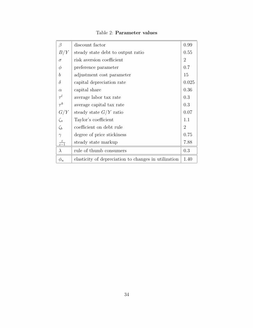
Table 2: Parameter values

β discount factor 0.99

B/Y steady state debt to output ratio 0.55

σ risk aversion coefficient 2

φ preference parameter 0.7

b adjustment cost parameter 15

δ capital depreciation rate 0.025

α capital share 0.36

τ l average labor tax rate 0.3

τ k average capital tax rate 0.3

G/Y steady state G/Y ratio 0.07

ζπ Taylor’s coefficient 1.1

ζb coefficient on debt rule 2

γ degree of price stickiness 0.75εε−1 steady state markup 7.88

λ rule of thumb consumers 0.3

φu elasticity of depreciation to changes in utilization 1.40

34

Table 3: Monte Carlo Experiment: DSGE Model Shock Standard Deviations

Shock Standard Deviation

Unanticipated Defense Shock 0.03

Anticipated Defense Shock 0.03

Measurement Errors 0.01

Notes : This table reports the standard deviations of the shocks used to generate the datain the Monte Carlo experiment of Section 6.

Table 4: Monte Carlo Correlations

Mean 2.5th and 97.5th Percentiles

0.84 [0.78,0.88]

Notes : This table reports the correlations between the MFEV shock and the narrative-based shock and the true defense shock series, computed from 2000 Monte Carlo simulationsof the model of Section 5.1. The MFEV shock was identified using the empirical MFEVidentification method and the narrative-based shock is the VAR innovation in the artificiallyconstructed narrative-based news shock measure constructed by adding a measurement errorto the true news shock series. The benchmark case pertain to a Monte Carlo exercise in whichthe narrrative-based series was included in the VAR, whereas the second row corresponds tothe exercise in which this series was excluded from the VAR.

35

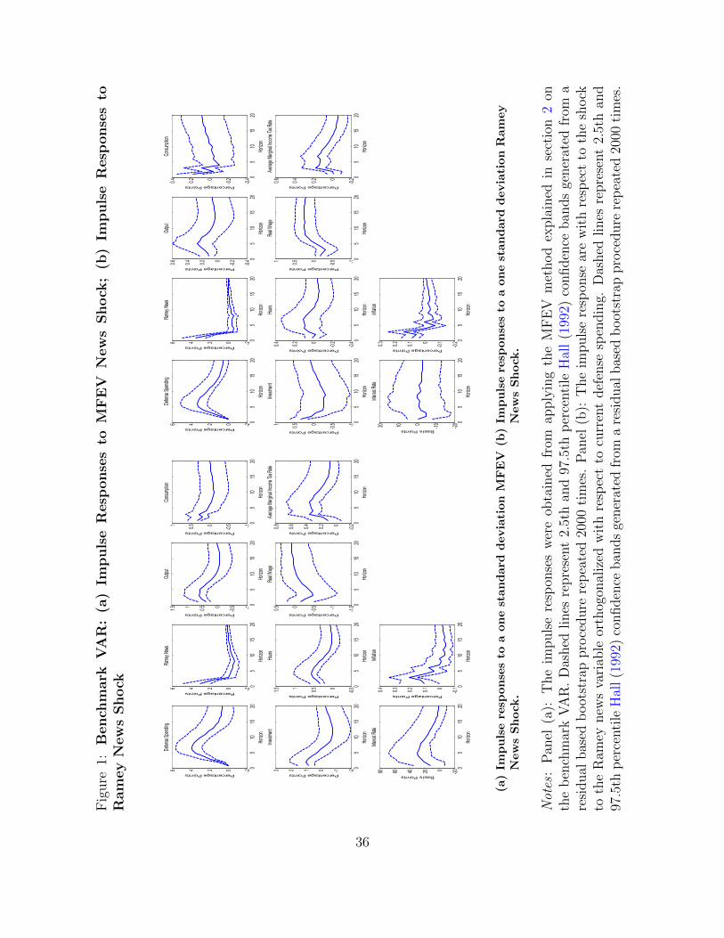
Fig

ure

1:B

en

chm

ark

VA

R:

(a)

Impuls

eR

esp

onse

sto

MF

EV

New

sShock

;(b

)Im

puls

eR

esp

onse

sto

Ram

ey

New

sShock

05

1015

20-20246

Rame

y Ne

ws

Horizon

Percentage Points

05

1015

20-1-0.500.511.5

Outpu

t

Horiz

on

Percentage Points

05

1015

20-1-0.500.51

Consum

ption

Horiz

on

Percentage Points

05

1015

20-2-10123

Investm

ent

Horizon

Percentage Points

05

1015

20-0.500.511.5

Hours

Horizon

Percentage Points

05

1015

20-1.5-1-0.500.5

Real Wag

e

Horiz

on

Percentage Points

05

1015

20-0.200.2

0.4

0.6

0.8

Average Ma

rgina

l Inco

me Ta

x Rate

Horiz

on

Percentage Points

05

1015

20-20246

Defense Sp

endin

g

Horizon

Percentage Points

05

1015

20-20020406080

Interest R

ate

Horizon

Basis Points

05

1015

20-0.100.1

0.2

0.3

0.4

Inflation

Horizon

Percentage Points

(a)

Imp

uls

ere

spon

ses

toa

on

est

an

dard

devia

tion

MF

EV

New

sS

hock

.

05

1015

20-20246

Rame

y Ne

ws

Horiz

on

Percentage Points

05

1015

20-0

.4

-0.200.2

0.4

0.6

Outpu

t

Horiz

on

Percentage Points

05

1015

20-0

.4

-0.200.2

0.4

Cons

umpti

on

Horiz

on

Percentage Points

05

1015

20-1-0.500.51

Inve

stmen

t

Horiz

on

Percentage Points

05

1015

20-0

.4

-0.200.2

0.4

Hour

s

Horiz

on

Percentage Points

05

1015

20-1-0.500.51

Real

Wag

e

Horiz

on

Percentage Points

05

1015

20-0

.200.2

0.4

0.6

Aver

age

Marg

inal In

come

Tax R

ate

Horiz

on

Percentage Points

05

1015

20-20246

Defe

nse

Spen

ding

Horiz

on

Percentage Points

05

1015

20-2

0

-1001020

Inter

est R

ate

Horiz

on

Basis Points

05

1015

20-0

.2

-0.100.1

0.2

0.3

Infla

tion

Horiz

on

Percentage Points

(b)

Imp

uls

ere

spon

ses

toa

on

est

an

dard

devia

tion

Ram

ey

New

sS

hock

.

Notes

:P

anel

(a):

The

impuls

ere

spon

ses

wer

eob

tain

edfr

omap

ply

ing

the

MF

EV

met

hod

expla

ined

inse

ctio

n2

onth

eb

ench

mar

kV

AR

.D

ashed

lines

repre

sent

2.5t

han

d97

.5th

per

centi

leH

all

(199

2)co

nfiden

ceban

ds

gener

ated

from

are

sidual

bas

edb

oot

stra

ppro

cedure

rep

eate

d20

00ti

mes

.P

anel

(b):

The

impuls

ere

spon

sear

ew

ith

resp

ect

toth

esh

ock

toth

eR

amey

new

sva

riab

leor

thog

onal

ized

wit

hre

spec

tto

curr

ent

def

ense

spen

din

g.D

ashed

lines

repre

sent

2.5t

han

d97

.5th

per

centi

leH

all

(199

2)co

nfiden

ceban

ds

gener

ated

from

are

sidual

bas

edb

oot

stra

ppro

cedure

rep

eate

d20

00ti

mes

.

36

Figure 2: The Share of Forecast Error Variance Attributable to MFEV NewsShocks and Ramey’s News Shocks.

0 5 10 15 2040

50

60

70

80

90

100Ramey News

Horizon

Proportion of Forecast Error

MFEV Defense News Shock

Ramey News Shock

0 5 10 15 200

5

10

15

20

25Output

Horizon

Proportion of Forecast Error

0 5 10 15 200

5

10

15

20

25Consumption

Horizon

Proportion of Forecast Error

0 5 10 15 200

5

10

15

20Investment

Horizon

Proportion of Forecast Error

0 5 10 15 200

5

10

15

20

25

30Hours

Horizon

Proportion of Forecast Error

0 5 10 15 200

2

4

6

8Real Wage

Horizon

Proportion of Forecast Error

0 5 10 15 200

5

10

15

20

25Average Marginal Income Tax Rate

HorizonProportion of Forecast Error

0 5 10 15 200

10

20

30

40

50

60Defense Spending

Horizon

Proportion of Forecast Error

0 5 10 15 200

5

10

15Interest Rate

Horizon

Proportion of Forecast Error

0 5 10 15 200

5

10

15

20

25Inflation

Horizon

Proportion of Forecast Error

Notes : The MFEV news shock corresponds to that from figure 1a whereas the Ramey newsshock corresponds to that from figure 1b.

37

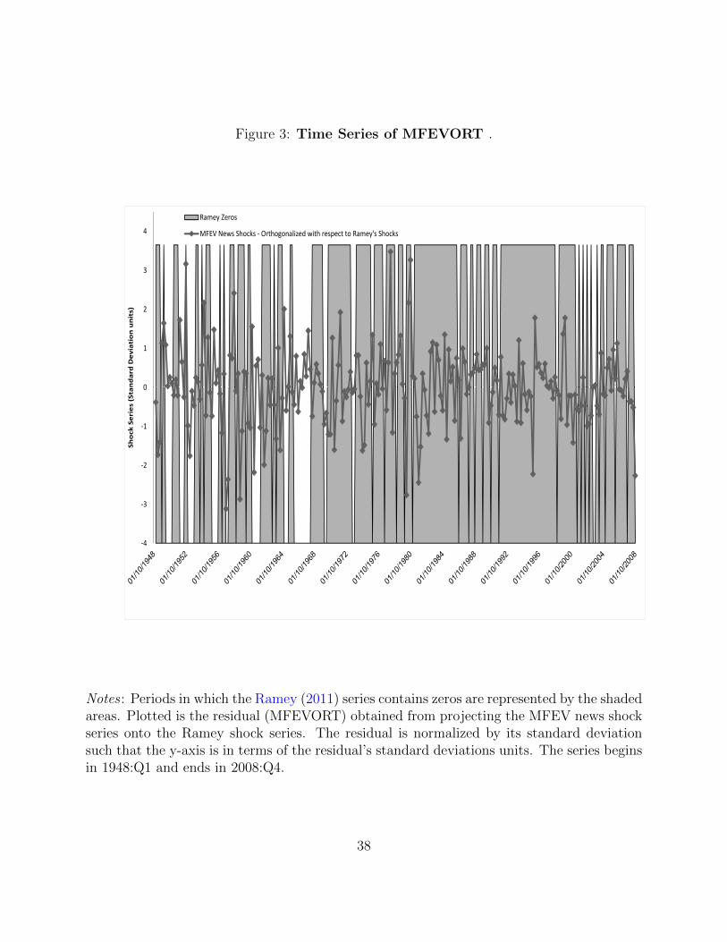
Figure 3: Time Series of MFEVORT .

-4

-3

-2

-1

0

1

2

3

4

Sh

ock

Se

rie

s (

Sta

nd

ard

De

via

tio

n u

nit

s)

Ramey Zeros

MFEV News Shocks - Orthogonalized with respect to Ramey's Shocks

Notes : Periods in which the Ramey (2011) series contains zeros are represented by the shadedareas. Plotted is the residual (MFEVORT) obtained from projecting the MFEV news shockseries onto the Ramey shock series. The residual is normalized by its standard deviationsuch that the y-axis is in terms of the residual’s standard deviations units. The series beginsin 1948:Q1 and ends in 2008:Q4.

38

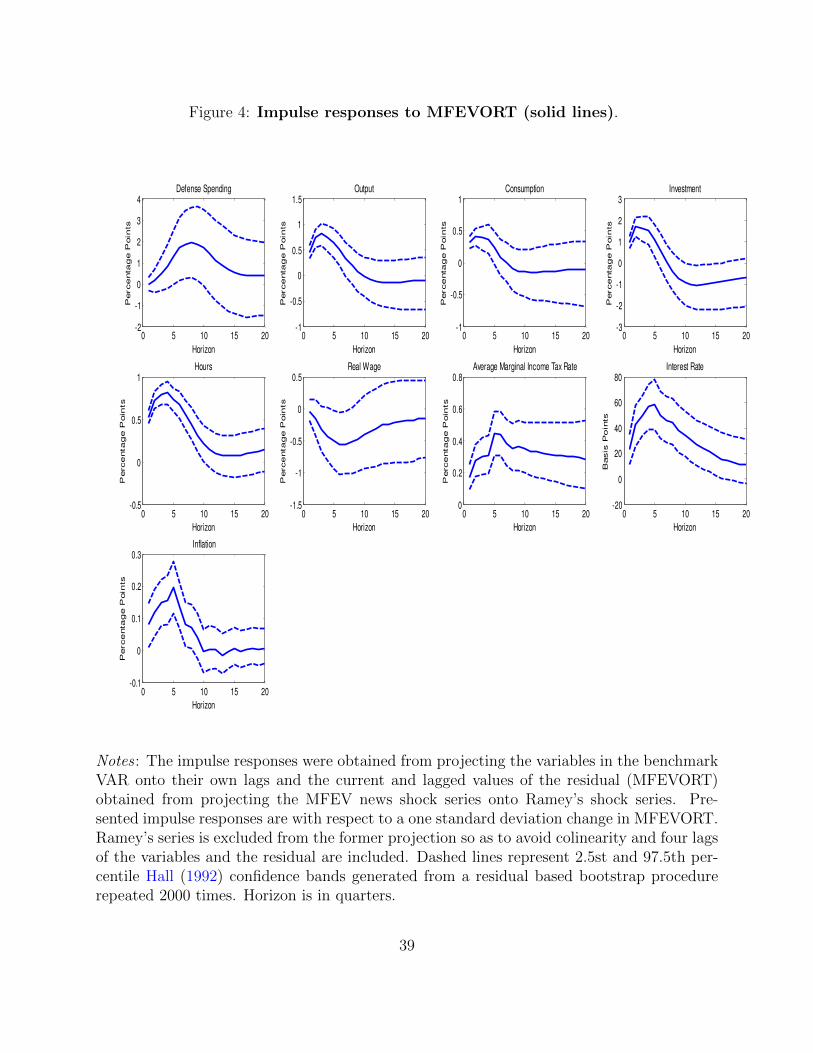
Figure 4: Impulse responses to MFEVORT (solid lines).

0 5 10 15 20-1

-0.5

0

0.5

1

1.5Output

Horizon

Perce

nta

ge P

oin

ts

0 5 10 15 20-1

-0.5

0

0.5

1Consumption

Horizon

Perce

nta

ge P

oin

ts

0 5 10 15 20-3

-2

-1

0

1

2

3Investment

Horizon

Perce

nta

ge P

oin

ts

0 5 10 15 20-0.5

0

0.5

1Hours

Horizon

Perce

nta

ge P

oin

ts

0 5 10 15 20-1.5

-1

-0.5

0

0.5Real Wage

Horizon

Perce

nta

ge P

oin

ts

0 5 10 15 200

0.2

0.4

0.6

0.8Average Marginal Income Tax Rate

Horizon

Perce

nta

ge P

oin

ts

0 5 10 15 20-2

-1

0

1

2

3

4Defense Spending

Horizon

Perce

nta

ge P

oin

ts

0 5 10 15 20-20

0

20

40

60

80Interest Rate

Horizon

Basis

Po

ints

0 5 10 15 20-0.1

0

0.1

0.2

0.3Inflation

Horizon

Perce

nta

ge P

oin

ts

Notes : The impulse responses were obtained from projecting the variables in the benchmarkVAR onto their own lags and the current and lagged values of the residual (MFEVORT)obtained from projecting the MFEV news shock series onto Ramey’s shock series. Pre-sented impulse responses are with respect to a one standard deviation change in MFEVORT.Ramey’s series is excluded from the former projection so as to avoid colinearity and four lagsof the variables and the residual are included. Dashed lines represent 2.5st and 97.5th per-centile Hall (1992) confidence bands generated from a residual based bootstrap procedurerepeated 2000 times. Horizon is in quarters.

39

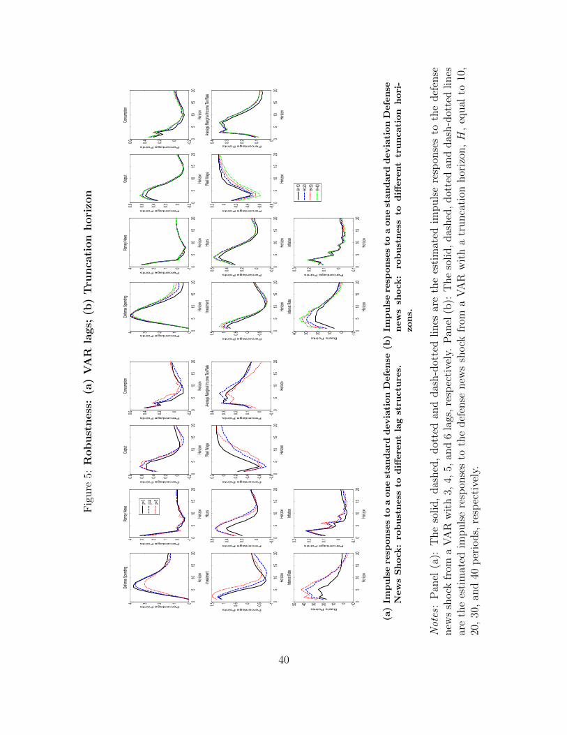
Fig

ure

5:R

ob

ust

ness

:(a

)V

AR

lags;

(b)

Tru

nca

tion

hori

zon

05

1015

20-101234

Ramey News

Horizon

Percentage Points

p=3

p=4

p=5

05

1015

20-0.200.2

0.4

0.6

0.8

Output

Horizon

Percentage Points

05

1015

20-0.200.2

0.4

0.6

Consumption

Horizon

Percentage Points

05

1015

20-1-0.500.511.5

Investment

Horizon

Percentage Points

05

1015

20-0.200.2

0.4

0.6

Hours

Horizon

Percentage Points

05

1015

20-0.8

-0.6

-0.4

-0.200.2

Real Wage

Horizon

Percentage Points

05

1015

20-0.100.1

0.2

0.3

0.4

Average Marginal Income Tax Rate

Horizon

Percentage Points

05

1015

2001234

Defense Spending

Horizon

Percentage Points

05

1015

20-1001020304050

Interest Rate

Horizon

Basis Points

05

1015

20-0.100.1

0.2

0.3

Inflation

Horizon

Percentage Points

(a)

Imp

uls

ere

spon

ses

toa

on

est

an

dard

devia

tion

Defe

nse

New

sS

hock

:ro

bu

stness

tod

iffere

nt

lag

stru

ctu

res.

05

1015

20-101234

Rame

y New

s

Horiz

on

Percentage Points

H=10

H=20

H=30

H=40

05

1015

20-0.200.2

0.4

0.6

0.8

Outpu

t

Horiz

on

Percentage Points

05

1015

20-0.200.2

0.4

0.6

Consum

ption

Horizon

Percentage Points

05

1015

20-1-0.500.511.5

Investm

ent

Horiz

on

Percentage Points

05

1015

20-0.200.2

0.4

0.6

Hours

Horiz

on

Percentage Points

05

1015

20-0.8

-0.6

-0.4

-0.200.2

Real Wag

e

Horiz

on

Percentage Points

05

1015

2000.1

0.2

0.3

0.4

Average Ma

rgina

l Inco

me Ta

x Rate

Horizon

Percentage Points

05

1015

2001234

Defense Sp

endin

g

Horiz

on

Percentage Points

05

1015

20-10010203040

Inter

est R

ate

Horiz

on

Basis Points

05

1015

20-0.100.1

0.2

0.3

Inflation

Horiz

on

Percentage Points

(b)

Imp

uls

ere

spon

ses

toa

on

est

an

dard

devia

tion

Defe

nse

new

ssh

ock

:ro

bu

stn

ess

tod

iffere

nt

tru

ncati

on

hori

-zon

s.

Notes

:P

anel

(a):

The

solid,

das

hed

,dot

ted

and

das

h-d

otte

dlines

are

the

esti

mat

edim

puls

ere

spon

ses

toth

edef

ense

new

ssh

ock

from

aV

AR

wit

h3,

4,5,

and

6la

gs,

resp

ecti

vely

.P

anel

(b):

The

solid,

das

hed

,dot

ted

and

das

h-d

otte

dlines

are

the

esti

mat

edim

puls

ere

spon

ses

toth

edef

ense

new

ssh

ock

from

aV

AR

wit

ha

trunca

tion

hor

izon

,H

,eq

ual

to10

,20

,30

,an

d40

per

iods,

resp

ecti

vely

.

40

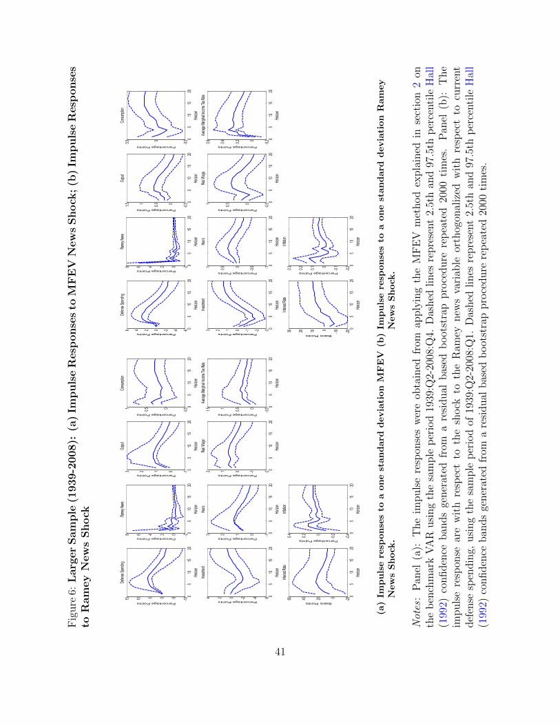
Fig

ure

6:L

arg

er

Sam

ple

(1939-2

008):

(a)

Impuls

eR

esp

onse

sto

MF

EV

New

sShock

;(b

)Im

puls

eR

esp

onse

sto

Ram

ey

New

sShock

05

1015

20-202468

Rame

y New

s

Horiz

on

Percentage Points

05

1015

20-10123

Outpu

t

Horiz

on

Percentage Points

05

1015

20-0

.500.51

Cons

umpti

on

Horiz

on

Percentage Points

05

1015

20-6-4-2024

Inve

stmen

t

Horiz

on

Percentage Points

05

1015

20-10123

Hour

s

Horiz

on

Percentage Points

05

1015

20-2-1012

Real

Wag

e

Horiz

on

Percentage Points

05

1015

20-0

.500.511.5

Aver

age

Marg

inal In

come

Tax R

ate

Horiz

on

Percentage Points

05

1015

20-1

0-5051015De

fens

e Sp

endin

g

Horiz

on

Percentage Points

05

1015

20-2

00204060In

teres

t Rate

Horiz

on

Basis Points

05

1015

20-0

.4

-0.200.2

0.4

Infla

tion

Horiz

on

Percentage Points

(a)

Imp

uls

ere

spon

ses

toa

on

est

an

dard

devia

tion

MF

EV

New

sS

hock

.

05

1015

20-202468

Ramey N

ews

Horizon

Percentage Points

05

1015

20-0.500.511.5

Output

Horizon

Percentage Points

05

1015

20-0.500.5

Consumption

Horizon

Percentage Points

05

1015

20-3-2-10123

Investm

ent

Horizon

Percentage Points

05

1015

20-1-0.500.51

Hours

Horizon

Percentage Points

05

1015

20-0.500.51

Real Wage

Horizon

Percentage Points

05

1015

20-0.200.2

0.4

0.6

Average Marginal Income Tax Rate

Horizon

Percentage Points

05

1015

20-6-4-20246

Defense Spending

Horizon

Percentage Points

05

1015

20-20

-100102030

Interest Rate

Horizon

Basis Points

05

1015

20-0.2

-0.100.1

0.2

0.3

Inflation

Horizon

Percentage Points

(b)

Imp

uls

ere

spon

ses

toa

on

est

an

dard

devia

tion

Ram

ey

New

sS

hock

.

Notes

:P

anel

(a):

The

impuls

ere

spon

ses

wer

eob

tain

edfr

omap

ply

ing

the

MF

EV

met

hod

expla

ined

inse

ctio

n2

onth

eb

ench

mar

kV

AR

usi

ng

the

sam

ple

per

iod

1939

:Q2-

2008

:Q4.

Das

hed

lines

repre

sent

2.5t

han

d97

.5th

per

centi

leH

all

(199

2)co

nfiden

ceban

ds

gener

ated

from

are

sidual

bas

edb

oot

stra

ppro

cedure

rep

eate

d20

00ti

mes

.P

anel

(b):

The

impuls

ere

spon

sear

ew

ith

resp

ect

toth

esh

ock

toth

eR

amey

new

sva

riab

leor

thog

onal

ized

wit

hre

spec

tto

curr

ent

def

ense

spen

din

g,usi

ng

the

sam

ple

per

iod

of19

39:Q

2-20

08:Q

1.D

ashed

lines

repre

sent

2.5t

han

d97

.5th

per

centi

leH

all

(199

2)co

nfiden

ceban

ds

gener

ated

from

are

sidual

bas

edb

oot

stra

ppro

cedure

rep

eate

d20

00ti

mes

.

41

Fig

ure

7:P

ost

-Kore

aW

ar

Sam

ple

(1955-2

008):

(a)

Impuls

eR

esp

onse

sto

MF

EV

New

sShock

;(b

)Im

puls

eR

esp

onse

sto

Ram

ey

New

sShock

05

1015

20-0.500.511.5

Rame

y New

s

Horiz

on

Percentage Points

05

1015

20-1-0.500.511.5

Outpu

t

Horiz

on

Percentage Points

05

1015

20-1-0.500.51

Cons

umption

Horiz

on

Percentage Points

05

1015

20-4-2024

Investm

ent

Horiz

on

Percentage Points

05

1015

20-0.500.511.5

Hours

Horiz

on

Percentage Points

05

1015

20-3-2-101

Real

Wag

e

Horiz

on

Percentage Points

05

1015

20-0.4

-0.200.2

0.4

0.6

Averag

e Ma

rgina

l Inco

me Ta

x Rate

Horiz

on

Percentage Points

05

1015

20-101234

Defense Sp

endin

g

Horiz

on

Percentage Points

05

1015

20-50050100

150

Inter

est R

ate

Horiz

on

Basis Points

05

1015

20-0.200.2

0.4

0.6

Inflation

Horiz

on

Percentage Points

(a)

Imp

uls

ere

spon

ses

toa

on

est

an

dard

devia

tion

MF

EV

New

sS

hock

.

05

1015

20-0

.500.511.52

Rame

y New

s

Horiz

on

Percentage Points

05

1015

20-0

.4

-0.200.2

0.4

0.6

Outpu

t

Horiz

on

Percentage Points

05

1015

20-0

.4

-0.200.2

0.4

0.6

Cons

umpti

on

Horiz

on

Percentage Points

05

1015

20-1-0.500.511.52

Inve

stmen

t

Horiz

on

Percentage Points

05

1015

20-0

.6

-0.4

-0.200.2

Hour

s

Horiz

on

Percentage Points

05

1015

20-0

.500.51

Real

Wag

e

Horiz

on

Percentage Points

05

1015

20-0

.4

-0.200.2

0.4

Aver

age

Marg

inal In

come

Tax R

ate

Horiz

on

Percentage Points

05

1015

20-0

.500.511.52

Defe

nse

Spen

ding

Horiz

on

Percentage Points

05

1015

20-3

0

-20

-100102030

Inter

est R

ate

Horiz

on

Basis Points

05

1015

20-0

.15-0.1

-0.050

0.050.

1In

flatio

n

Horiz

on

Percentage Points

(b)

Imp

uls

ere

spon

ses

toa

on

est

an

dard

devia

tion

Ram

ey

New

sS

hock

.

Notes

:P

anel

(a):

The

impuls

ere

spon

ses

wer

eob

tain

edfr

omap

ply

ing

the

MF

EV

met

hod

expla

ined

inse

ctio

n2

onth

eb

ench

mar

kV

AR

usi

ng

the

sam

ple

per

iod

1955

:Q1-

2008

:Q4.

Das

hed

lines

repre

sent

2.5t

han

d97

.5th

per

centi

leH

all

(199

2)co

nfiden

ceban

ds

gener

ated

from

are

sidual

bas

edb

oot

stra

ppro

cedure

rep

eate

d20

00ti

mes

.P

anel

(b):

The

impuls

ere

spon

sear

ew

ith

resp

ect

toth

esh

ock

toth

eR

amey

new

sva

riab

leor

thog

onal

ized

wit

hre

spec

tto

curr

ent

def

ense

spen

din

g,usi

ng

the

sam

ple

per

iod

of19

55:Q

1-20

08:Q

1.D

ashed

lines

repre

sent

2.5t

han

d97

.5th

per

centi

leH

all

(199

2)co

nfiden

ceban

ds

gener

ated

from

are

sidual

bas

edb

oot

stra

ppro

cedure

rep

eate

d20

00ti

mes

.

42

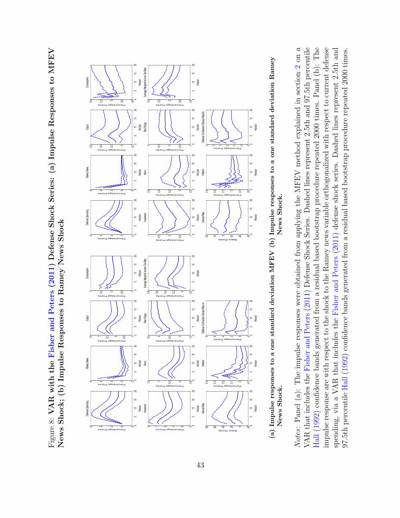
Fig

ure

8:V

AR

wit

hth

eF

isher

and

Pete

rs(2

011)

Defe

nse

Shock

Seri

es:

(a)

Impuls

eR

esp

onse

sto

MF

EV

New

sShock

;(b

)Im

puls

eR

esp

onse

sto

Ram

ey

New

sShock

05

1015

20-20246

Rame

y New

s

Horiz

on

Percentage Points

05

1015

20-1-0.500.511.5

Outpu

t

Horiz

on

Percentage Points

05

1015

20-1-0.500.51

Consum

ption

Horizon

Percentage Points

05

1015

20-3-2-1012

Investm

ent

Horiz

on

Percentage Points

05

1015

20-0.500.511.5

Hours

Horiz

on

Percentage Points

05

1015

20-1.5-1-0.500.5

Real Wag

e

Horiz

on

Percentage Points

05

1015

20-0.200.2

0.4

0.6

0.8

Average Ma

rgina

l Inco

me Ta

x Rate

Horizon

Percentage Points

05

1015

20-20246

Defense Sp

endin

g

Horiz

on

Percentage Points

05

1015

20-20020406080

Inter

est R

ate

Horiz

on

Basis Points

05

1015

20-0.100.1

0.2

0.3

0.4

Inflation

Horiz

on

Percentage Points

05

1015

20-202468

Defense Co

ntrac

tors E

xcess R

eturns

Horiz

on

Percentage Points

(a)

Imp

uls

ere

spon

ses

toa

on

est

an

dard

devia

tion

MF

EV

New

sS

hock

.

05

1015

20-20246

Rame

y New

s

Horiz

on

Percentage Points

05

1015

20-0

.200.2

0.4

0.6

Outpu

t

Horiz

on

Percentage Points

05

1015

20-0

.4

-0.200.2

0.4

Cons

umpti

on

Horiz

on

Percentage Points

05

1015

20-1-0.500.51

Inve

stmen

t

Horiz

on

Percentage Points

05

1015

20-0

.200.2

0.4

0.6

Hour

s

Horiz

on

Percentage Points

05

1015

20-1-0.500.51

Real

Wag

e

Horiz

on

Percentage Points

05

1015

20-0

.4

-0.200.2

0.4

Aver

age

Marg

inal In

come

Tax R

ate

Horiz

on

Percentage Points

05

1015

20-20246

Defe

nse

Spen

ding

Horiz

on

Percentage Points

05

1015

20-3

0

-20

-1001020

Inter

est R

ate

Horiz

on

Basis Points

05

1015

20-0

.2

-0.100.1

0.2

0.3

Infla

tion

Horiz

on

Percentage Points

05

1015

20-3-2-10123

Defe

nse

Contr

actor

s Exc

ess R

eturn

s

Horiz

on

Percentage Points

(b)

Imp

uls

ere

spon

ses

toa

on

est

an

dard

devia

tion

Ram

ey

New

sS

hock

.

Notes

:P

anel

(a):

The

impuls

ere

spon

ses

wer

eob

tain

edfr

omap

ply

ing

the

MF

EV

met

hod

expla

ined

inse

ctio

n2

ona

VA

Rth

atin

cludes

the

Fis

her

and

Pet

ers

(201

1)D

efen

seShock

Ser

ies.

Das

hed

lines

repre

sent

2.5t

han

d97

.5th

per

centi

leH

all

(199

2)co

nfiden

ceban

ds

gener

ated

from

are

sidual

bas

edb

oot

stra

ppro

cedure

rep

eate

d20

00ti

mes

.P

anel

(b):

The

impuls

ere

spon

sear

ew

ith

resp

ect

toth

esh

ock

toth

eR

amey

new

sva

riab

leor

thog

onal

ized

wit

hre

spec

tto

curr

ent

def

ense

spen

din

g,via

aV

AR

that

incl

udes

the

Fis

her

and

Pet

ers

(201

1)def

ense

shock

seri

es.

Das

hed

lines

repre

sent

2.5t

han

d97

.5th

per

centi

leH

all

(199

2)co

nfiden

ceban

ds

gener

ated

from

are

sidual

bas

edb

oot

stra

ppro

cedure

rep

eate

d20

00ti

mes

.

43

Figure 9: VAR Without the Ramey (2011) Series: Impulse responses to a onestandard deviation Defense News Shock (solid lines).

0 5 10 15 20-1

-0.5

0

0.5

1

1.5

2Output

Horizon

Perce

nta

ge P

oin

ts

0 5 10 15 20-1

-0.5

0

0.5

1

1.5Consumption

Horizon

Perce

nta

ge P

oin

ts

0 5 10 15 20-4

-2

0

2

4Investment

Horizon

Perce

nta

ge P

oin

ts

0 5 10 15 20-0.5

0

0.5

1

1.5

2Hours

Horizon

Perce

nta

ge P

oin

ts

0 5 10 15 20-2.5

-2

-1.5

-1

-0.5

0

0.5Real Wage

Horizon

Perce

nta

ge P

oin

ts

0 5 10 15 20-0.5

0

0.5

1Average Marginal Income Tax Rate

Horizon

Perce

nta

ge P

oin

ts

0 5 10 15 20-2

0

2

4

6

8Defense Spending

Horizon

Perce

nta

ge P

oin

ts

0 5 10 15 20-20

0

20

40

60

80

100Interest Rate

Horizon

Basis

Po

ints

0 5 10 15 20-0.2

0

0.2

0.4

0.6

0.8Inflation

Horizon

Perce

nta

ge P

oin

ts

Notes : The impulse responses were obtained from applying the MFEV method explainedin section 2 on a VAR that excludes the Ramey (2011) news series. Dashed lines represent2.5th and 97.5th percentile Hall (1992) confidence bands generated from a residual basedbootstrap procedure repeated 2000 times. Horizon is in quarters.

44

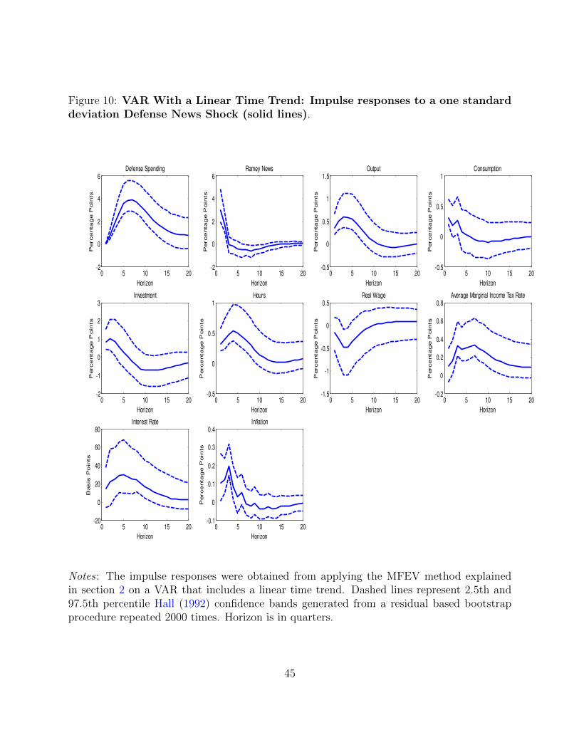
Figure 10: VAR With a Linear Time Trend: Impulse responses to a one standarddeviation Defense News Shock (solid lines).

0 5 10 15 20-2

0

2

4

6Ramey News

Horizon

Perce

nta

ge P

oin

ts

0 5 10 15 20-0.5

0

0.5

1

1.5Output

Horizon

Perce

nta

ge P

oin

ts

0 5 10 15 20-0.5

0

0.5

1Consumption

Horizon

Perce

nta

ge P

oin

ts

0 5 10 15 20-2

-1

0

1

2

3Investment

Horizon

Perce

nta

ge P

oin

ts

0 5 10 15 20-0.5

0

0.5

1Hours

Horizon

Perce

nta

ge P

oin

ts

0 5 10 15 20-1.5

-1

-0.5

0

0.5Real Wage

Horizon

Perce

nta

ge P

oin

ts

0 5 10 15 20-0.2

0

0.2

0.4

0.6

0.8Average Marginal Income Tax Rate

Horizon

Perce

nta

ge P

oin

ts

0 5 10 15 20-2

0

2

4

6Defense Spending

Horizon

Perce

nta

ge P

oin

ts

0 5 10 15 20-20

0

20

40

60

80Interest Rate

Horizon

Basis

P

oin

ts

0 5 10 15 20-0.1

0

0.1

0.2

0.3

0.4Inflation

Horizon

Perce

nta

ge P

oin

ts

Notes : The impulse responses were obtained from applying the MFEV method explainedin section 2 on a VAR that includes a linear time trend. Dashed lines represent 2.5th and97.5th percentile Hall (1992) confidence bands generated from a residual based bootstrapprocedure repeated 2000 times. Horizon is in quarters.

45

Figure 11: The Cross-Correlation between the MFEV News Shock and Lags/Leadsof Other Structural Shocks.

-4 -2 0 2 4-0.4

-0.2

0

0.2

0.4Romer-Romer Monetary Policy Shocks

Lags

Corre

latio

n

-4 -2 0 2 4-0.4

-0.2

0

0.2

0.4Romer-Romer Tax Shocks

Lags

Corre

latio

n

-4 -2 0 2 4-0.4

-0.2

0

0.2

0.4Oil Shocks

Lags

Corre

latio

n

-4 -2 0 2 4-0.4

-0.2

0

0.2

0.4Barsky-Sims TFP News Shocks

Lags

Corre

lati

on

-4 -2 0 2 4-0.4

-0.2

0

0.2

0.4Baker-Bloom-Davis Economic Policy Uncertainty Shocks

Lags

Corre

lati

on

-4 -2 0 2 4-0.4

-0.2

0

0.2

0.4Mertens-Ravn Unanticipated Tax Shocks

Lags

Corre

lati

on

-4 -2 0 2 4-0.4

-0.2

0

0.2

0.4Mertens-Ravn Anticipated Tax Shocks

Lags

Corre

latio

n

Correlation

95th and 5th Percentiles

Notes : The solid line is the cross-correlation and the dashed lines represent the 95% asymp-totic confidence interval. The other shocks are the Romer and Romer (2004) monetary policyshock measure, Romer and Romer (2010) tax shock measure, shock to the real price of oil,the TFP news shock from Barsky and Sims (2011), the innovation to the U.S. economicpolicy uncertainty index of Baker et al. (2012), and the unanticipated and anticipated taxshocks constructed by Mertens and Ravn (2012). Apart from the Barsky and Sims (2011)TFP news shock series which was used in its raw form, all other shocks were constructed asthe residuals of univariate regressions of each of the four variables on four lags.

46

Figure 12: The Cross-Correlation between MFEVORT and Lags/Leads of OtherStructural Shocks.

-4 -2 0 2 4-0.4

-0.2

0

0.2

0.4Romer-Romer Monetary Policy Shocks

Lags

Corre

latio

n

-4 -2 0 2 4-0.4

-0.2

0

0.2

0.4Romer-Romer Tax Shocks

Lags

Corre

latio

n

-4 -2 0 2 4-0.4

-0.2

0

0.2

0.4Oil Shocks

Lags

Corre

latio

n-4 -2 0 2 4

-0.4

-0.2

0

0.2

0.4Barsky-Sims TFP News Shocks

Lags

Corre

lati

on

-4 -2 0 2 4-0.4

-0.2

0

0.2

0.4Baker-Bloom-Davis Economic Policy Uncertainty Shocks

Lags

Corre

lati

on

-4 -2 0 2 4-0.4

-0.2

0

0.2

0.4Mertens-Ravn Unanticipated Tax Shocks

Lags

Corre

lati

on

-4 -2 0 2 4-0.4

-0.2

0

0.2

0.4Mertens-Ravn Anticipated Tax Shocks

Lags

Corre

latio

n

Correlation

95th and 5th Percentiles

Notes : The solid line is the cross-correlation and the dashed lines represent the 95% asymp-totic confidence interval. MFEVORT is the component of the MFEV news shock that isorthogonal to the Ramey news shock. The macroeconomic shocks with which the cross-correlations are computed are identical to those considered in Figure 11.

47

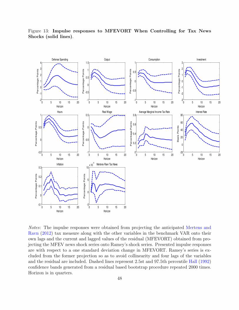
Figure 13: Impulse responses to MFEVORT When Controlling for Tax NewsShocks (solid lines).

0 5 10 15 20-1

-0.5

0

0.5

1

1.5Output

Horizon

Perce

nta

ge P

oin

ts

0 5 10 15 20-1

-0.5

0

0.5

1Consumption

Horizon

Perce

nta

ge P

oin

ts

0 5 10 15 20-3

-2

-1

0

1

2

3Investment

Horizon

Perce

nta

ge P

oin

ts

0 5 10 15 20-0.5

0

0.5

1Hours

Horizon

Perce

nta

ge P

oin

ts

0 5 10 15 20-1

-0.5

0

0.5Real Wage

Horizon

Perce

nta

ge P

oin

ts

0 5 10 15 200

0.2

0.4

0.6

0.8Average Marginal Income Tax Rate

Horizon

Perce

nta

ge P

oin

ts

0 5 10 15 20-2

-1

0

1

2

3

4Defense Spending

Horizon

Perce

nta

ge P

oin

ts

0 5 10 15 20-20

0

20

40

60

80Interest Rate

Horizon

Basis

P

oin

ts

0 5 10 15 20-0.1

0

0.1

0.2

0.3Inflation

Horizon

Perce

nta

ge P

oin

ts

0 5 10 15 20-5

0

5

10x 10

-4Mertens-Ravn Tax News

Horizon

Perce

nta

ge P

oin

ts

Notes : The impulse responses were obtained from projecting the anticipated Mertens andRavn (2012) tax measure along with the other variables in the benchmark VAR onto theirown lags and the current and lagged values of the residual (MFEVORT) obtained from pro-jecting the MFEV news shock series onto Ramey’s shock series. Presented impulse responsesare with respect to a one standard deviation change in MFEVORT. Ramey’s series is ex-cluded from the former projection so as to avoid collinearity and four lags of the variablesand the residual are included. Dashed lines represent 2.5st and 97.5th percentile Hall (1992)confidence bands generated from a residual based bootstrap procedure repeated 2000 times.Horizon is in quarters.

48

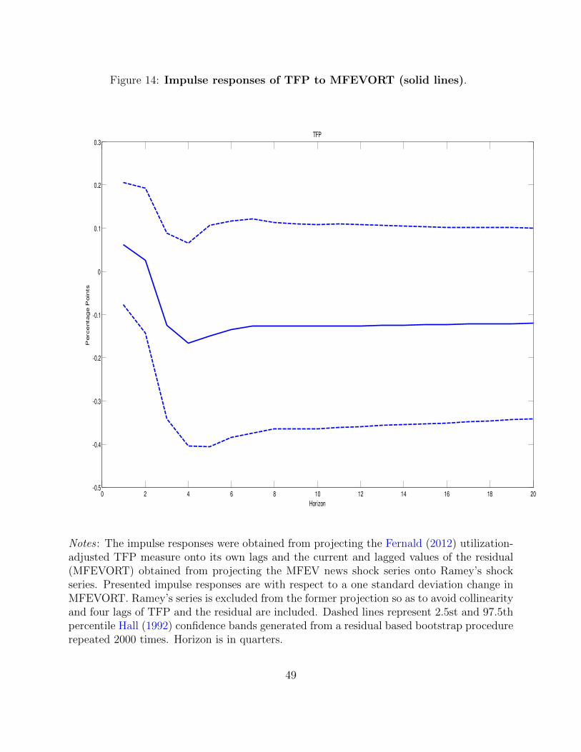
Figure 14: Impulse responses of TFP to MFEVORT (solid lines).

0 2 4 6 8 10 12 14 16 18 20-0.5

-0.4

-0.3

-0.2

-0.1

0

0.1

0.2

0.3TFP

Horizon

Perce

nta

ge P

oin

ts

Notes : The impulse responses were obtained from projecting the Fernald (2012) utilization-adjusted TFP measure onto its own lags and the current and lagged values of the residual(MFEVORT) obtained from projecting the MFEV news shock series onto Ramey’s shockseries. Presented impulse responses are with respect to a one standard deviation change inMFEVORT. Ramey’s series is excluded from the former projection so as to avoid collinearityand four lags of TFP and the residual are included. Dashed lines represent 2.5st and 97.5thpercentile Hall (1992) confidence bands generated from a residual based bootstrap procedurerepeated 2000 times. Horizon is in quarters.

49

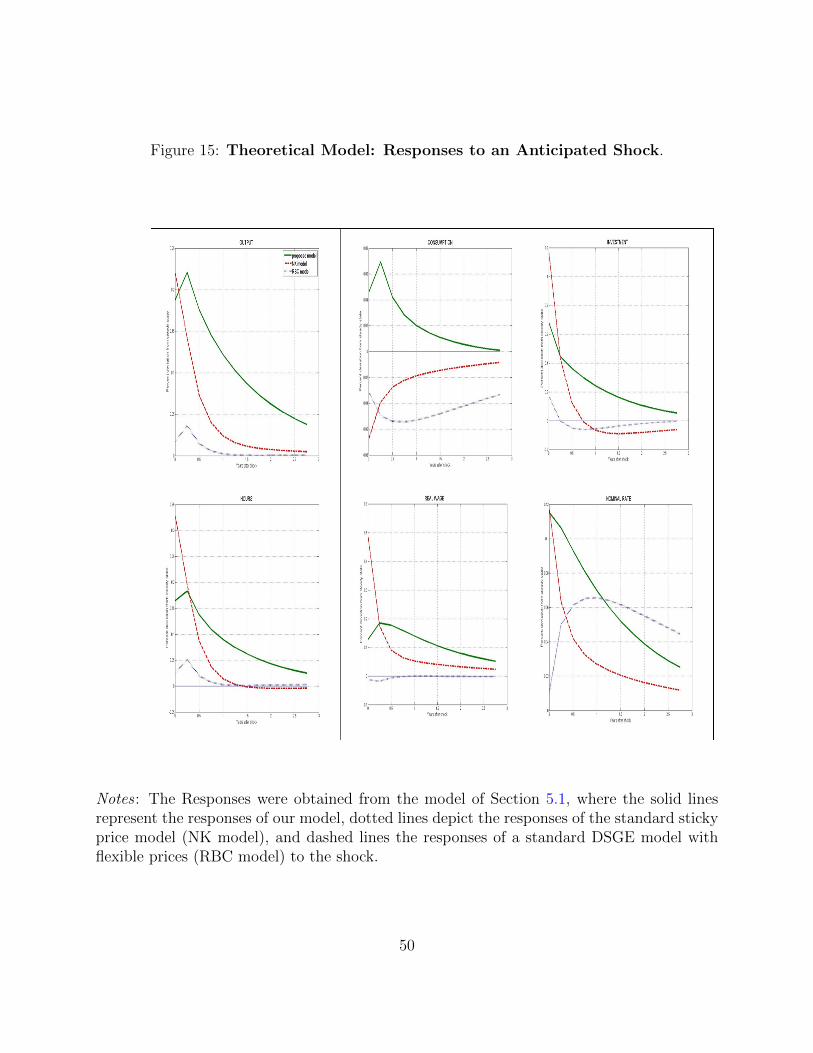
Figure 15: Theoretical Model: Responses to an Anticipated Shock.

Notes : The Responses were obtained from the model of Section 5.1, where the solid linesrepresent the responses of our model, dotted lines depict the responses of the standard stickyprice model (NK model), and dashed lines the responses of a standard DSGE model withflexible prices (RBC model) to the shock.

50

Figure 16: Theoretical Model: Quantification of the Propagation MechanismsInduced by Sticky Prices, Jaimovich and Rebelo (2009) Preferences, and Ruleof Thumb Consumers.

Notes : The Responses were obtained from the model of Section 5.1, where each columncorresponds to a model in which the relevant feature is absent from the model.

51

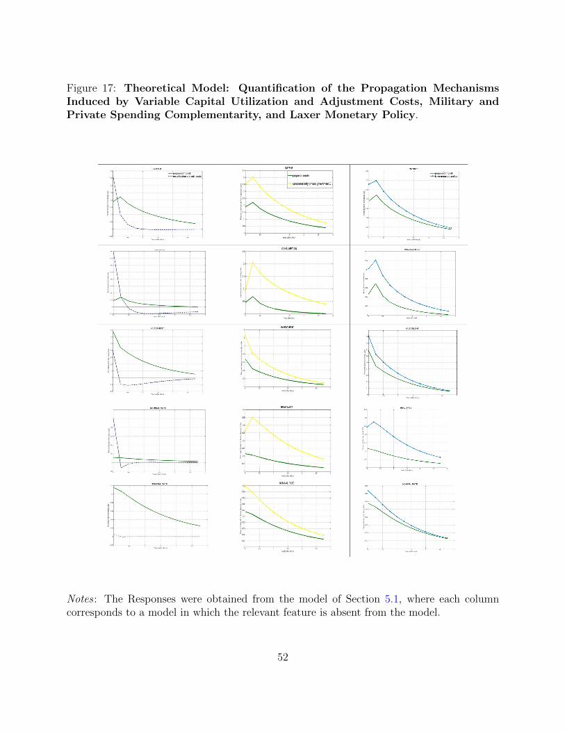
Figure 17: Theoretical Model: Quantification of the Propagation MechanismsInduced by Variable Capital Utilization and Adjustment Costs, Military andPrivate Spending Complementarity, and Laxer Monetary Policy.

Notes : The Responses were obtained from the model of Section 5.1, where each columncorresponds to a model in which the relevant feature is absent from the model.

52

Figure 18: Monte Carlo Evidence: Estimated Impulse Responses to IdentifiedNews Shock.

0 5 10 15 20-1

0

1

2

3

4Defense Spending

Horizon

Perce

nta

ge D

evia

tio

n

Model

Estimated

0 5 10 15 20-0.2

0

0.2

0.4

0.6

0.8Output

Horizon

Perce

nta

ge D

evia

tio

n

0 5 10 15 20-0.2

0

0.2

0.4

0.6Consumption

Horizon

Perce

nta

ge D

evia

tio

n

0 5 10 15 20-0.5

0

0.5

1

1.5

2Investment

Horizon

Perce

nta

ge D

evia

tio

n

0 5 10 15 20-0.2

0

0.2

0.4

0.6Hours

Horizon

Perce

nta

ge D

evia

tio

n

0 5 10 15 20-0.1

0

0.1

0.2

0.3Inflation

Horizon

Perce

nta

ge P

oin

t D

evia

tio

n

0 5 10 15 20-0.2

0

0.2

0.4

0.6Interest rate

HorizonP

erce

ntag

e P

oin

t D

evia

tio

n

0 5 10 15 20-0.1

-0.05

0

0.05

0.1Tax Rate

Horizon

Perce

ntag

e P

oin

t D

evia

tio

n

0 5 10 15 20-0.5

0

0.5

1Real Wage

Horizon

Perce

nta

ge D

evia

tio

n

Notes : The figures are based on 2000 Monte Carlo simulations of the model of Section5.1 where in each simulation the MFEV shock was identified using the empirical MFEVidentification method. The solid line represents the true model impulse responses, the dashedline is the average estimated impulse response to the MFEV shock across Monte Carloreplications, and the dotted lines are the 97.5th and 2.5th estimated percentiles.

53