Christopher Dougherty EC220 - Introduction to econometrics (chapter 3) Slideshow: exercise 3.5 Original citation: Dougherty, C. (2012) EC220 - Introduction

Christopher Dougherty

EC220 - Introduction to econometrics (chapter 3)Slideshow: exercise 3.5

Original citation:

Dougherty, C. (2012) EC220 - Introduction to econometrics (chapter 3). [Teaching Resource]

© 2012 The Author

This version available at: http://learningresources.lse.ac.uk/129/

Available in LSE Learning Resources Online: May 2012

This work is licensed under a Creative Commons Attribution-ShareAlike 3.0 License. This license allows the user to remix, tweak, and build upon the work even for commercial purposes, as long as the user credits the author and licenses their new creations under the identical terms. http://creativecommons.org/licenses/by-sa/3.0/

http://learningresources.lse.ac.uk/

http://learningresources.lse.ac.uk/

http://creativecommons.org/licenses/by-sa/3.0/

3.5 Explain why the intercept in the regression of EEARNon ES is equal to zero.

1

EXERCISE 3.5

This exercise relates to the Frisch–Lovell–Waugh procedure for graphing the relationship between the dependent variable and one of the explanatory variables in a multiple regression model.

The model was an earnings function with earnings hypothesized to be determined by years of schooling and years of work experience.

2

EXERCISE 3.5

. reg EARNINGS S EXP

Source | SS df MS Number of obs = 540-------------+------------------------------ F( 2, 537) = 67.54 Model | 22513.6473 2 11256.8237 Prob > F = 0.0000 Residual | 89496.5838 537 166.660305 R-squared = 0.2010-------------+------------------------------ Adj R-squared = 0.1980 Total | 112010.231 539 207.811189 Root MSE = 12.91

------------------------------------------------------------------------------ EARNINGS | Coef. Std. Err. t P>|t| [95% Conf. Interval]-------------+---------------------------------------------------------------- S | 2.678125 .2336497 11.46 0.000 2.219146 3.137105 EXP | .5624326 .1285136 4.38 0.000 .3099816 .8148837 _cons | -26.48501 4.27251 -6.20 0.000 -34.87789 -18.09213------------------------------------------------------------------------------

EXPSINGSNEAR 56.068.249.26ˆ

3

To represent the relationship between EARNINGS and S graphically, we first regress EARNINGS on EXP and save the residuals, which we call EEARN.

EXERCISE 3.5

. reg EARNINGS EXP


------------------------------------------------------------------------------ EARNINGS | Coef. Std. Err. t P>|t| [95% Conf. Interval]-------------+---------------------------------------------------------------- EXP | .2414715 .1398002 1.73 0.085 -.0331497 .5160927 _cons | 15.55527 2.442468 6.37 0.000 10.75732 20.35321------------------------------------------------------------------------------

. predict EEARN, resid

4

Then we do the same with S. We regress it on EXP and save the residuals as ES.

EXERCISE 3.5

. reg S EXP


------------------------------------------------------------------------------ S | Coef. Std. Err. t P>|t| [95% Conf. Interval]-------------+---------------------------------------------------------------- EXP | -.1198454 .0231436 -5.18 0.000 -.1653083 -.0743826 _cons | 15.69765 .4043447 38.82 0.000 14.90337 16.49194------------------------------------------------------------------------------

. predict ES, resid

5

A plot of EEARN and ES then gives a proper graphical representation of the relationship between EARNINGS and S, controlling for the effects of EXP.

EXERCISE 3.5

-20

0

20

40

60

80

-8 -6 -4 -2 0 2 4 6

ES (schooling residuals)

EEARN

(e

arn

ing

s r

es

idu

als

)

Here is the regression of EEARN on ES. The intercept is 8.10e–09, which means 8.10x10–9, or –0.00000000810, effectively zero. What is the reason for this?

6

EXERCISE 3.5

. reg EEARN ES


------------------------------------------------------------------------------ EEARN | Coef. Std. Err. t P>|t| [95% Conf. Interval]-------------+---------------------------------------------------------------- ES | 2.678125 .2334325 11.47 0.000 2.219574 3.136676 _cons | 8.10e-09 .5550284 0.00 1.000 -1.090288 1.090288------------------------------------------------------------------------------

. reg EEARN ES

Source | SS df MS Number of obs = 570---------+------------------------------ F( 1, 568) = 21.21 Model | 1256.44239 1 1256.44239 Prob > F = 0.0000Residual | 33651.2873 568 59.2452241 R-squared = 0.0360---------+------------------------------ Adj R-squared = 0.0343 Total | 34907.7297 569 61.3492613 Root MSE = 7.6971

------------------------------------------------------------------------------ EEARN | Coef. Std. Err. t P>|t| [95% Conf. Interval]---------+-------------------------------------------------------------------- ES | .7390366 .1604802 4.605 0.000 .4238296 1.054244 _cons | -5.99e-09 .3223957 0.000 1.000 -.6332333 .6332333------------------------------------------------------------------------------

EXERCISE 4.5

XbYb 21

uXY 21

7

In the simple regression model, the intercept is calculated as the mean of the dependent variable minus b2 times the mean of the explanatory variable.

. reg EEARN ES



EXERCISE 4.5

XbYb 21

00 221 bESbEEARNb

uXY 21

8

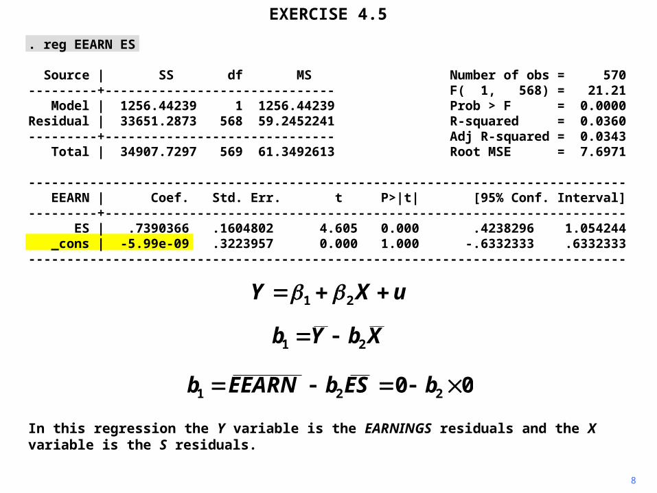
In this regression the Y variable is the EARNINGS residuals and the X variable is the S residuals.

. reg EEARN ES



9

The means of both of these are zero because residuals from OLS regressions always have zero means. Hence the intercept must be zero.

EXERCISE 4.5

XbYb 21

00 221 bESbEEARNb

uXY 21

Copyright Christopher Dougherty 1999–2006. This slideshow may be freely copied for personal use.

26.06.06

Documents

Christopher Dougherty EC220 - Introduction to econometrics (chapter 3) Slideshow: exercise 3.5 Original citation: Dougherty, C. (2012) EC220 - Introduction