HAL Id: halshs-02057137https://halshs.archives-ouvertes.fr/halshs-02057137v2

Preprint submitted on 17 Mar 2021

HAL is a multi-disciplinary open accessarchive for the deposit and dissemination of sci-entific research documents, whether they are pub-lished or not. The documents may come fromteaching and research institutions in France orabroad, or from public or private research centers.

L’archive ouverte pluridisciplinaire HAL, estdestinée au dépôt et à la diffusion de documentsscientifiques de niveau recherche, publiés ou non,émanant des établissements d’enseignement et derecherche français ou étrangers, des laboratoirespublics ou privés.

Choosing Unemployment Benefits:the Role of AdverseSelection and Moral Hazard

Laura Khoury

To cite this version:Laura Khoury. Choosing Unemployment Benefits:the Role of Adverse Selection and Moral Hazard.2021. �halshs-02057137v2�

WORKING PAPER N° 2019 – 13

Choosing Unemployment Benefits: the Role of Adverse Selection and Moral Hazard

Laura Khoury

JEL Codes: J08, J65, J68, H31 Keywords: Unemployment, moral hazard, adverse selection, insurance design.

Choosing Unemployment Benefits:the Role of Adverse Selection and Moral Hazard∗

Laura Khoury†

Abstract

Most unemployment insurance (UI) schemes mandate a single benefit schedule,while little empirical findings support this mandate. In this paper, I exploit aFrench program where workers are given a choice between two different UI sched-ules, providing an ideal setup to evaluate both moral hazard and selection intoUI. Using high-quality administrative data, I measure significant adverse selectionby relating the entitlement choice with the characteristics of the insured. Moralhazard is even larger, as shown by a fuzzy regression discontinuity design using aneligibility criterion: choosing a short schedule with higher average benefits increasesunemployment duration by six months.

Keywords: Unemployment, moral hazard, adverse selection, insurance design

JEL Codes: J08, J65, J68, H31

∗I am grateful to Spenser Bastani, Luc Behaghel, Antoine Bozio, Paul Brandily, Clément Brebion,Thomas Ericson, François Fontaine, Thomas Giebe, Andreas Haller, Jonas Kolsrud, Camille Landais,Thomas Le Barbanchon, Katrine Løken, Armando Meier, Bertil Tungodden, Arne Uhlendorff, and An-drea Weber for their help and comments, as well as to numerous participants in workshops and seminars.I would also like to thank the Unédic for hosting me and providing me access to the data, and my col-leagues in the Analysis and Studies Department of Unédic for their help, especially Claire Goarant,with whom I worked on a note on the same topic. I acknowledge the support of the EUR grant ANR-17-EURE-0001. An earlier version of this paper circulated under the title "Generosity versus DurationTrade-Off and the Optimization Ability of the Unemployed".

†Norwegian School of Economics, Helleveien 30, 5045 Bergen, Norway. Email: laura.khoury@nhh.no

1 Introduction

The very principle of offering mandated public unemployment insurance (UI) is rarelyquestioned. This is because theory has well-established that a mandate can solve theunderprovision of insurance in a competitive private equilibrium that is due to adverseselection (Rothschild and Stiglitz, 1976; Akerlof, 1978).1 In line with this theoreticalargument, we observe that most existing UI schemes offer a single mandated schedule atthe national level. However, empirical evidence supporting this argument in the specificcontext of UI is lacking, the main challenge being that mandated schemes do not allowresearchers to observe insurance choices.2

In this paper, I take advantage of an uncommon UI program that lets jobseekerschoose between two benefit schedules. Both schedules differ horizontally in benefit level,duration, and time profile, and vertically, since the total sum of potential benefits collectedis higher in one option. This allows me to measure both the adverse selection and moralhazard costs of UI benefits in a unique setting. Under this program, jobseekers can choosebetween either a long length of time with on average lower benefits, or a shorter length oftime with on average higher benefits. Leveraging high-quality administrative data, I firstassess the extent of moral hazard after a simultaneous change in the level, duration, andtime profile of benefits (while those parameters are generally analyzed separately). To doso, I measure the causal impact of choosing a shorter unemployment compensation withon average higher benefits using a regression discontinuity design (RDD) on an eligibilitythreshold.3 Second, I identify adverse selection into UI by relating the choice of theinsured to her initial level of risk.4 While previous empirical literature on UI has mainlyfocused on moral hazard, evidence on the empirical existence of selection into UI remainsscarce. I measure adverse selection and separate it from moral hazard using the estimatefrom the RDD.

The program under study, called the option right (OR), was introduced in Francein 2015, to allow unemployed workers alternating short employment and unemploymentspells to better smooth their income. More precisely, it targets people who received

1Adverse selection may arise when there is heterogeneity in the level of risk, and individuals haveprivate information on their risk type (Rothschild and Stiglitz, 1976; Akerlof, 1978). The intuition isthat the insurer prices according to the average risk level, as he has no information on individual risktype. The presence of high-risk types makes this average premium too costly for low-risk types, who exitthe market. As low-risk types leave, the average premium goes up, driving ever more low-risk types outof the market, and ending up in its collapse.

2Sweden, Denmark, Finland and Iceland are the only countries where choice is widely available inthe UI system.

3Noneligibles cannot choose and are offered the default option, which is the long schedule with onaverage lower benefits. Moral hazard in the paper refers to the behavioral change in response to thisincrease in the average level of benefits entailed by the high-short-benefit schedule, although it implies ahigher benefit at the start of the spell and a lower benefit later in the spell.

4In this setting, adverse selection is assessed by linking the initial unemployment risk to the choiceof the low-long option which also offers a higher total amount of benefits.

1

low UI benefits in the past, which they have not exhausted, and who are returning tounemployment. These workers are given a choice between either (i) starting with theremainder of the former compensation followed by their new one or (ii) directly usingtheir new right (computed on the basis of only their last employment spell). Becausethe remainder of the former right is associated with a low level of benefits, and the newright with a higher one,5 it implies that the first option offers the worker a low levelof initial benefits, followed by a higher compensation, for a long total potential benefitduration (PBD). The second option provides the worker with higher benefits immediatelyfor a shorter total PBD (see Figure ?? for an example). For the sake of simplicity, in theremainder of the paper, the first option will be referred to as the low-long-benefit schedule,and the second one as the high-short-benefit schedule.6 The RDD is then comparingworkers offered a choice between both schedules (below the cutoff) with workers offeredonly the long and low-benefit schedule, which is the default option.7 Moral hazard, in thepaper, therefore refers to the behavioral change in response to the increase in the averagelevel of benefits entailed by the high-short-benefit schedule, although it implies a higherbenefit at the start of the spell and a lower benefit later in the spell. From an insuranceperspective, what makes the worker better off is a priori unclear. The two schedules areboth horizontally- and vertically-differentiated: opting for the high-short-benefit scheduleis equivalent to trading tomorrow’s benefits off for today’s benefits. At the same time,retaining the remainder of the former right reduces the risk of exhausting benefits andpotentially provides a larger total amount of benefits. If the premium paid does notdirectly differ between both options,8 choosing the low-long benefit implies an extensionof the coverage at the expense of lower benefits in the short run. Having an option thatunambiguously entails a higher total amount of benefits – but with a lower average one– makes such a setting particularly appropriate for measuring both adverse selection andmoral hazard.

To understand better the determinants of the OR take-up, I first provide descriptiveevidence on the characteristics of the unemployed choosing the high-short-benefit option.The likely existence of private information about employment prospects encourages totest for the presence of adverse selection and try to quantify its magnitude. Leveragingrich administrative data and machine learning methods, I predict the unemploymentduration of each individual in my sample, capturing most of the information available tothe worker when he makes his insurance choice. Performing the correlation test between

5This is by construction of the eligibility conditions.6This is a simplification because the first option allows the jobseeker to receive higher benefits at the

end of the UI spell, and because the second option entails a shorter benefit duration, but which can stillbe long in absolute terms.

7People above the eligibility threshold could also be eligible if they meet other conditions, that I amnot able to observe. For that reason, the design is fuzzy. For simplicity, I will refer to workers below thethreshold as having a choice and workers above the threshold as not having a choice.

8The contributions paid during employment spells are the same in both options.

2

insurance coverage and the predicted unemployment duration, as opposed to the realizedone, presumably provides a better test of adverse selection, one that is not confoundedwith moral hazard. To quantify moral hazard, I compare people on either side of a benefitcutoff who differ in their ability to choose their schedule. This fuzzy RDD allows to studythe response of unemployed people to a change in the level and potential duration ofbenefits. In theory, the effect of both parameters is expected to go in opposite directions,as most of the literature has found a positive relationship between the level of benefitsand unemployment duration on the one hand, and PBD and unemployment duration onthe other (see Schmieder and Von Wachter (2016) for a review). Therefore, the net jointimpact is ambiguous. I measure this joint impact, both in financial and employmentterms. Because I have no information on the job found after leaving unemployment,my main outcome variable is the duration of the unemployment spell. Finally, I usethe estimate of moral hazard that I obtain from the RDD to decompose the observeddifference in risk between adverse selection and moral hazard.

The analysis points to five main results. (i) I measure significant adverse selection,since individuals with the highest initial unemployment risk tend to select the longestcoverage. (ii) Workers able to choose the high-benefit option have a much longer unem-ployment spell duration, indicating sizable moral hazard. (iii) However, the effect seemsto fade out over time. Workers offered a choice do not differ in terms of total number ofdays on benefits on a longer time horizon. (iv) Findings suggest that additional numberof days unemployed in the short run are not used to find better-quality jobs. Workersoffered a choice work more frequently while being unemployed,9 but this type of partialemployment is often associated with part-time and temporary contracts.10 (v) Finally,when individuals with the highest initial unemployment risk are offered a choice, theyalso suffer a larger negative impact. This suggests, together with a heterogeneity analy-sis, that the unemployed already experiencing difficulties in the labor market – the lessskilled, less educated, and younger ones – are the most harmed by the OR. This raisessome questions on the welfare cost of allowing the unemployed to choose their insurancecoverage. The increase in unemployment duration for workers choosing the high-short-benefits is strikingly large (i.e. a 157-day response), but is in line with the literatureshowing that workers are generally more sensitive to the level than the duration of bene-fits (see Schmieder et al. (2016) for a review of elasticities) and that the moral hazard costof UI is higher early in the spell (Kolsrud et al., 2018). Moreover, workers on which theresponse is estimated may exhibit a particularly large response since (i) they self-selectinto high-short benefits; (ii) but are still entitled to a long benefit duration; (iii) and are

9The French UI scheme allows jobseekers to keep receiving part of their UI benefits when they goback to work if their earnings and working time are below a certain threshold.

10However, a definitive answer to this question cannot be established. I do not observe the qualityof the job found at the end of the unemployment spell, but only that of the jobs taken during theunemployment spell.

3

likely to be liquidity-constrained.This paper relates to several strands of the literature. Although theoretical work (Ak-

erlof, 1978; Rothschild and Stiglitz, 1976) has preceded empirical evidence, there is nowa large body of papers testing for the presence of selection in insurance markets. Recentpapers go beyond the correlation test (Chiappori and Salanie, 2000) that mixes adverseselection with moral hazard, as both predict that individuals with the highest coveragehave higher claims. They use quasi-experimental variations in prices to reconstruct thedemand and cost curves in various insurance markets, such as health insurance (Einav etal., 2010; Finkelstein et al., 2019). Finkelstein and Poterba (2002, 2004, 2014) have usedthe fact that moral hazard is unlikely in annuity markets, as it would entail a behavioralresponse on life duration to income in the form of an annuity. However, because such anassumption does not hold in the UI context, and because private schemes are virtuallynonexistent, precluding the observation of insurance choices, empirical evidence on thepresence of selection into UI is lacking.11 There are two notable exceptions.12 Hendren(2017) develops a methodology that does not rely on observing insurance choices. Heuses elicited beliefs about job loss to demonstrate that no private UI scheme can be sus-tained, as a complement of the existing public UI scheme in the US, because workers’private information on their level of risk would entail too much selection. Landais etal. (2021) use the coexistence of minimum mandated coverage with private additionalinsurance that can be purchased on a voluntary basis in Sweden to confirm the presenceof adverse selection, controlling for moral hazard, and explore the welfare consequences ofa mandate. My setting differs from Hendren (2017) because I directly observe insurancechoices, that I can relate to the initial unemployment risk of the workers. My settingalso differs from Landais et al. (2021) because the two insurance contracts vary not onlyin the extent of coverage, but also in how it is allocated over time.13 This horizontaldifferentiation partly affects the interpretation of adverse selection and moral hazard: Ishow that there is still adverse selection in a context where both options do not differ interms of premium,14 but where benefits of the option with the highest coverage are lower

11Reviewing the empirical literature on adverse selection in social insurances, Chetty and Finkelstein(2013) (p. 134) explain “In contrast to the study of selection in annuity and health insurance marketsthere is, to our knowledge, a dearth of work on adverse selection in several settings where there are im-portant social insurance programs including disability insurance, unemployment insurance, and worker’scompensation”.

12Parsons et al. (2003) also investigate the extent of selection in the Danish context of voluntary UI.Using a multinomial logit model, they show that workers purchasing UI have a higher unemployment risk.However, their estimation is complicated by the fact that UI purchase depends on union membership andthe eligibility to high social assistance benefits, that they try to take into account using the sample ofswitchers into and out of the UI scheme. They also control for moral hazard by measuring unemploymentrisk the first year of membership, during which workers are not eligible for benefits yet. However, theprospect of being able to receive UI benefits in the near future could still influence workers’ behavior.The use of quasi experimental methods in my paper presumably provides a more robust measure of moralhazard.

13As there is a simultaneous change in replacement rate, benefit duration and profile.14It means that the willingness to pay does not influence the insurance decision.

4

in the first period. It suggests that riskier individuals prioritize the length of the coverageor minimize the risk of having no benefit at all. The moral hazard response is complexand measured on multiple outcomes, both in the short and long run. Because the neteffect of having the high-short benefit option is an increase in unemployment duration,it suggests that less risky individuals are more sensitive to the level than the duration ofbenefits in their search behavior.

This paper also contributes to the optimal unemployment insurance literature (Baily,1978; Chetty, 2006), as it explores the behavioral response of workers to different pa-rameters of UI, to measure its distortion cost on labor supply. A large literature hasquantified the distorting effect of UI generosity on unemployment duration or reservationwage (Meyer, 1988; Feldstein and Poterba, 1984; Van Ours and Vodopivec, 2006; Laliveet al., 2006; Lalive, 2007; Lalive et al., 2015; Le Barbanchon et al., 2017). Some authors(Landais, 2015; Kolsrud et al., 2018) have built on the initial framework to study theoptimal time profile of UI, drawing attention also to the duration of UI entitlements.Elasticities with respect to both the level and the duration of benefits are crucial toevaluating the cost and welfare effect of UI and to improve its design. This paper con-tributes to insights into this issue. Often examined separately, the analysis focuses hereon the combined effect of both parameters on labor market outcomes. Establishing whichof the two parameters prevails is important, especially for policymakers concerned withreforming UI by limiting behavioral responses. Moreover, this recent literature has alsohighlighted the importance of how UI benefits were allocated over time, as the moral haz-ard cost and insurance values are not likely to be constant throughout the unemploymentspell. In the setting I study, the high-benefit option amounts to an increase in benefitearly in the spell and a decrease to zero later in the spell.15 Given the large moral haz-ard cost triggered by the high-benefit option, this paper suggests that a declining profileis not optimal. This finding is consistent with Kolsrud et al. (2018) who find that themoral hazard cost of UI benefits is larger early in the spell, whereas the insurance valueis larger later in the spell, advocating for an inclining benefit profile. However, Lindnerand Reizer (2016) take advantage of an experiment in Hungary frontloading UI benefits,keeping constant the total UI benefit amount, and find opposite effects. The discrepancybetween these findings can be explained by the Hungarian reform being more salient, andpeople being more aware of future benefit cuts. My paper adds to this ongoing debate bydemonstrating the positive impact on unemployment duration of receiving high benefitsimmediately as opposed to an inclining benefit path.16

Choosing the short and high-benefit option can be related, to a certain extent, to risk15Unemployed workers choosing this option may qualify for social minima after the exhaustion point,

but will not necessarily because they are means-tested based on household income. Their level is alsogenerally lower than UI benefits.

16In the French context, the choice between both options was presented in rather complex terms, asa mix between the former and new entitlements, rather than as a choice between two benefit profiles.

5

aversion, present-biased preferences, or optimism. While I do not measure these parame-ters, several behavioral mechanisms can rationalize my results. For example, hyperbolictime preferences, with a low short-term discount parameter, could explain both the de-cision to opt for the short and high-benefit schedule and poor labor market outcomes.Indeed, it has been shown that unemployed people, especially at low levels of wages,exhibit hyperbolic time preferences (Paserman, 2008) and that impatience associatedwith hyperbolic time preferences has a negative impact on job search (DellaVigna andPaserman, 2005). Exploring another channel, Mueller et al. (2018) find that unemployedworkers in general, and the long-term unemployed in particular, are overoptimistic abouttheir employment prospects. Overoptimism can lead workers to choose the high-benefitschedule and to be overly selective and stay longer in unemployment. A further explo-ration of how OR choices could be used to estimate time discounting or risk aversion isleft to future work.

The remainder of the paper proceeds as follows. Section 2 describes the institutionalbackground as well as the data. Section 3 analyzes the determinants of the take-up andthe extent of selection. Section 4 estimates the impact of the OR on future labor marketoutcomes and investigates the magnitude of moral hazard and adverse selection. Section5 concludes.

2 Institutional setting and data

Institutional background – The option right was introduced as a corrective to the2014 UI Agreement17 because some unemployed people were adversely affected by it.Indeed, the 2014 Agreement introduced two principles: (i) the automatic resumption ofthe former right, meaning that a person taking a new job before exhausting his UI rightautomatically benefited from the remainder of his former right when again becomingunemployed; and (ii) the recharging of the right, meaning that, at the exhaustion pointof his former right, the worker was allowed to extend the entitlements based on his lastemployment spells.18 This mechanism was a way to use any employment spell, evenshort ones, to extend UI entitlements and maximize the coverage duration without anyinterruption to payments. However, this mechanism, meant to be more favorable, turnedout to have unintended consequences for workers whose last employment spell was highlypaid whereas the remainder of their former right was associated with a low daily benefit(DB). Making the resumption of the former right automatic at the end of the employmentspell would cause a large drop in income. This regulation has then been rectified by anamendment to the 2014 Agreement, which gave the possibility to these types of workers

17Amendment №1 of March 25, 2015 modifying the general regulation appended to the Conventionof May 14, 2014 on unemployment insurance.

18This holds once at least 150 hours of new employment spells that have never been used to computeany UI entitlements have accumulated.

6

to choose between benefiting from the remainder of their former right and then rechargingwith the new one or to jump directly to the new right associated with a higher averagedaily benefit. The first option implies longer benefits, starting with a low level andfollowed by higher ones. The second option leads to shorter benefits but starting directlywith the higher ones.19 This possibility to choose between both schedules, referred to asthe option right, was introduced in April 2015. Because the long and low-benefit scheduleis the default option, workers choosing the shorter unemployment compensation with onaverage higher benefits are referred to as takers.

The eligibility criteria to be granted this choice are the following: (i) having a residualfrom the former right; (ii) having worked at least 122 days or 610 hours since becomingeligible for the former right (corresponding to the minimum work history to open a UIright); (iii) having a DB associated with the former right no greater than 20e or havinga DB associated with the new right at least 30% greater than the former one. The lastcondition is the most crucial one and will allow the use of the thresholds as part of theidentification strategy. If eligible workers choose to exercise their OR, they will directlybenefit from their new right, and abandon the residual of their former right. An illustra-tive example can be found in Figure A1.

Data – I use administrative data from Unédic,20 the organization in charge of UIin France. It gathers all the information needed to compute UI entitlements, on thecharacteristics of the unemployment spell, as well as sociodemographic variables. It allowsme to follow the universe of registered unemployed workers with exhaustive informationon their successive unemployment spells for the period of interest (October 2014–May2017).21 However, two important data limitations should be noted.

First, although numerous details are available on the characteristics of the unemploy-ment spell, much less is known about what happens to unemployed people when theyleave the unemployment roll. If they interrupt the unemployment spell for any reason –sickness, maternity leave, a new job – while remaining registered, we can still follow themin the database even if we do not necessarily know the reason for the interruption. Thedatabase shows whether the person uses his right and/or receives benefits. If a personfails to remain registered, that person just disappears from the database, without neces-sarily providing the motive for the exit. With this information at hand and knowing thatwe are interested in employment spells of at least 122 days between two unemploymentspells, I define an unemployment spell as any period during which the person is registered

19For simplicity, in the remainder of the paper, the first option is referred to as the long and low-benefitschedule, and the second option is referred to as the short and high-benefit schedule.

20Union nationale interprofessionnelle pour l’emploi dans l’industrie et le commerce, the French na-tional interprofessional union for employment in industry and trade.

21October 2014–May 2017 is the main period of interest used throughout the paper. However, tocompute the unemployment probability of workers having started their UI spell during this period, Iextend the observation window to February 2018.

7

as unemployed with interruptions of less than 4 months. Any interruption of at least 4months, even if the person is still registered but does not use the right and is not paid,means the end of the unemployment spell, except if we know explicitly that it is for areason other than a return to the labor market. Then, I define as the paid unemploy-ment spell duration the addition of all the periods consumed and paid, and as the fullunemployment spell duration the addition of all registered periods, paid and unpaid.22

Second, for people eligible for the OR and choosing not to take it, nothing is knownabout the new right they could have opened, unless we observe a recharging in thefuture. Indeed, not to exercise means they are resuming their former right. Then, thedata do not record the opening of the new right they would have benefited from hadthey exercised it, and no information is available on this potential new right. This partialinformation implies that I am not able to compute the ratio of the new to the formerDB, and that I cannot take advantage of the 30% eligibility threshold. This limitationhas important consequences as it constrains the analysis to the 20e threshold, for whichonly the information on the former DB is needed. Nonetheless, knowing the value of thepotential new DB for these people would have been very informative in understandingthe exact terms of the trade-off faced by eligible people and to understand better thedeterminants of the take-up.

I build a final sample of people who began an unemployment spell from October 1,201423 who meet at least the first two eligibility criteria, that is, not having exhausteda former right and having worked at least 122 days between two unemployment spells.Among those, I can only observe whether the person is eligible but does not exercise hisOR under the 20e condition, and whether the OR is exercised under both conditions.Table B1 details the sample composition, with some proxies for the take-up rate, as thetrue rate could only be determined if we had the exact number of eligible people. I endup with a sample of 2,209,471 individuals, of whom more than 200,000 are eligible underthe 20e condition. Restricting ourselves to the 20e condition, the take-up rate is equalto 34%, although it may not perfectly reflect the overall take-up rate in the population.This rate may seem small, given the very low daily benefits associated with the formerright for this population (under 20e); however, there are many reasons for not exercisingthe OR that can stem from both the unemployed person and their caseworker. Indeed,survey data from Unédic reveals that caseworkers were sometimes reluctant to advertisethis choice and to argue in favor of opting for the new right, because they felt that it wasrisky for a population of workers generally experiencing difficulties in the labor market.

22By definition of unemployment spells, the unpaid periods within the spell are necessarily less than4 months. These periods are accounted for in the full unemployment spell duration computation only ifthe person maintains registration as unemployed and thus remains in the database.

23The amendment was passed on March 29, 2015 and applied from April 1, 2015 retrospectively onunemployment spells starting from October 1, 2014 onward. It means that a person who automaticallyresumed their former right between October 1, 2014 and April 1, 2015 could decide from the latter dateto exercise the OR and to switch directly to that new right.

8

In addition, unemployed people are not necessarily aware of the existence of such a possi-bility, and the default option is not to exercise the OR. By law, applying for the OR is atthe initiative of the jobseeker. That is why we observe an ascending trend in the numberof takers over the months, with a seasonality component, as displayed in Figure E1.

Description of the sample – Because of data limitations, this study focuses ona specific unemployed population with very low daily benefit (lower than or equal to20e). Yet, if specific, this population is nonnegligible, as it accounts for 12% of theflows to compensated unemployment as part of the main UI benefit.24 This populationis also particularly hard hit in the labor market because their benefits and thus theirprevious earnings were very low, which is often associated with low qualifications and alow probability of reemployment. Both their weight for all the people receiving UI benefitsas well as their situation in the labor market warrant our attention to their labor marketoutcomes. Moreover, while the results obtained cannot necessarily be extrapolated tothe whole unemployed population, they are of particular policy relevance if we believethe State should provide specific support to populations that are more distant from thelabor market.

Table 1 describes the characteristics of the eligible population under the 20e cutoffcompared to the population of noneligible nontakers.25 Consistent with their low benefitlevel, eligible workers are, on average, younger, more frequently female, less skilled andeducated. They also have a lower tenure and working hours, signaling their lower attach-ment to the labor market. Their initial potential benefit duration is also lower, indicatingless secure entitlements, in line with their lower tenure. Overall, eligible people underthe 20e condition are a more fragile population, namely more in difficulty in the labormarket compared with similar noneligible workers.

3 Determinants of the take-up

3.1 Descriptive evidence

The profile of takers – An exploration of the observable characteristics of eligibleworkers choosing the short and high-benefit option provides useful insights on the profileof the takers. Although not allowing us to fully understand their preferences, it canproxy for their prospects in the labor market, the way they anticipate them, and theirimpatience and risk aversion. In the following paragraphs, I describe: (i) the populationof takers under the 20e cutoff; (ii) the population of takers fulfilling the 20e but not

24As measured between January 2014 and March 2015.25This noneligible nontaker population refers to the population of people similar to eligible workers

except for the third eligibility condition, that is, having a former daily benefit lower than 20e. However,it may include workers eligible as part of the ratio criterion that I am not able to identify.

9

the 30% condition, on which I will measure the moral hazard response (later referredas the “complier” population); (iii) how they compare to eligible nontakers under the20e cutoff, to better understand the determinants of the take-up.

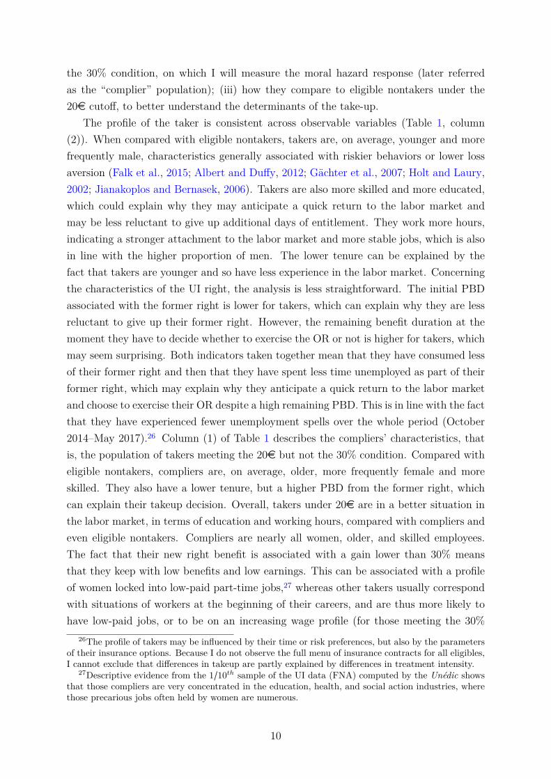
The profile of the taker is consistent across observable variables (Table 1, column(2)). When compared with eligible nontakers, takers are, on average, younger and morefrequently male, characteristics generally associated with riskier behaviors or lower lossaversion (Falk et al., 2015; Albert and Duffy, 2012; Gächter et al., 2007; Holt and Laury,2002; Jianakoplos and Bernasek, 2006). Takers are also more skilled and more educated,which could explain why they may anticipate a quick return to the labor market andmay be less reluctant to give up additional days of entitlement. They work more hours,indicating a stronger attachment to the labor market and more stable jobs, which is alsoin line with the higher proportion of men. The lower tenure can be explained by thefact that takers are younger and so have less experience in the labor market. Concerningthe characteristics of the UI right, the analysis is less straightforward. The initial PBDassociated with the former right is lower for takers, which can explain why they are lessreluctant to give up their former right. However, the remaining benefit duration at themoment they have to decide whether to exercise the OR or not is higher for takers, whichmay seem surprising. Both indicators taken together mean that they have consumed lessof their former right and then that they have spent less time unemployed as part of theirformer right, which may explain why they anticipate a quick return to the labor marketand choose to exercise their OR despite a high remaining PBD. This is in line with the factthat they have experienced fewer unemployment spells over the whole period (October2014–May 2017).26 Column (1) of Table 1 describes the compliers’ characteristics, thatis, the population of takers meeting the 20e but not the 30% condition. Compared witheligible nontakers, compliers are, on average, older, more frequently female and moreskilled. They also have a lower tenure, but a higher PBD from the former right, whichcan explain their takeup decision. Overall, takers under 20e are in a better situation inthe labor market, in terms of education and working hours, compared with compliers andeven eligible nontakers. Compliers are nearly all women, older, and skilled employees.The fact that their new right benefit is associated with a gain lower than 30% meansthat they keep with low benefits and low earnings. This can be associated with a profileof women locked into low-paid part-time jobs,27 whereas other takers usually correspondwith situations of workers at the beginning of their careers, and are thus more likely tohave low-paid jobs, or to be on an increasing wage profile (for those meeting the 30%

26The profile of takers may be influenced by their time or risk preferences, but also by the parametersof their insurance options. Because I do not observe the full menu of insurance contracts for all eligibles,I cannot exclude that differences in takeup are partly explained by differences in treatment intensity.

27Descriptive evidence from the 1/10th sample of the UI data (FNA) computed by the Unédic showsthat those compliers are very concentrated in the education, health, and social action industries, wherethose precarious jobs often held by women are numerous.

10

criterion).If eligible people under the 20e condition are a more fragile population, among them,

unemployed people who decide to exercise their OR appear to be less precarious, and toperform better in the labor market. Their higher education and qualifications can explainwhy they may be more confident in their labor market prospects and why they may favorthe UI’s generosity over the duration of the coverage.

The takeup decision – Table F1 runs a multivariate analysis of the probability ofbeing a complier or taker on the sample of eligibles, to examine the marginal effect of eachvariable, as they are potentially correlated. Only looking at predetermined characteristics,what seems the most important influence for probability of taking up the OR for eligiblesunder the 20e criterion is age, being female – both negatively correlated – and thelevel of qualifications, all else being equal.28 Interestingly, the level of education has anegative impact, whereas descriptive evidence (Table 1) shows that takers are, on average,more educated than eligible nontakers. The effect of education reverses when right’scharacteristics are added, while the coefficients on other predetermined characteristicsslightly decrease but stay of the same sign. The effect of age, gender and skills seems to bepartly captured by the positive and significant impact of working hours. The multivariateanalysis confirms previous descriptive evidence, where characteristics associated with ahigher taste for risk and better employment prospects influence positively the decision oftaking up the OR.

The picture looks different for compliers. Consistent with the higher proportion ofolder and female workers in this population, age and being a woman have both a posi-tive marginal impact, although the gender effect disappears when right’s characteristicsare added. The level of skills play a positive role in both regressions, and the effect ofright’s characteristics goes in the same direction as in the case of takers, although themagnitude of the coefficients is much smaller when looking at the probability of being acomplier. The decision to choose the short and high-benefit schedule among compliersdoes not seem to be necessarily related to better employment prospects, but is ratherconsistent with a profile of workers durably in part-time jobs with a medium number ofhours worked and fewer variations in their employment spell characteristics, and withvery low levels of benefits that make them presumably more sensitive to this parameter.

Characteristics of insurance options of takers – To gain a more complete pictureof the determinants of their choice, we can also look at the exact terms of the trade-offfaced by takers (Table B2). Takers are characterized by a new DB that is, on average,more than twice the former DB. This is not surprising because their choice to exercise

28The level of qualifications has a reversed scale, meaning that it has a positive impact on the prob-ability of being a taker.

11

the OR must be motivated by a high financial gain to compensate for the loss in termsof PBD. This ratio is even higher at close to 3 for takers having a former DB lower than20e, which is in line with the fact that, as their former DB is very low, the new one islikely to be much higher. However, compliers, who, by definition, have a ratio betweennew and former benefit lower than 1.3, gain only 18% in terms of level of benefits, onaverage.29 Row 3 of Table B2 indicates that the new PBD the taker is entitled to is 1.35longer than the PBD he gives up by exercising the OR. This ratio is lower in the caseof those taking under the 20e criterion. It is reasonable to believe that, at these verylow levels of DB, unemployed people are willing to give up a remaining PBD that, inproportion, represents more of their new PBD if it allows them to earn higher benefits.In other words, in the amount–duration trade-off, they are likely to put more weight onthe amount of their DB. For both types of takers, the total initial PBD associated withboth rights is almost the same, which can also motivate their choice. Indeed, they areoffered, as part of their new right, a PBD that is equal to what they were entitled to atthe beginning of their former right. By definition, if they are eligible for the OR, they arein a situation where they did not exhaust their former right. Then, based on their verylast experience, it makes sense for them to anticipate that they will not entirely consumetheir new right if they take it, and then, that they do not need a longer coverage, andthat they should exercise their OR.

However, the last row indicates that by doing so, takers choose to receive benefits fora period of time that is slightly more than half what they could have if they had notexercised the OR. In the case of compliers, they lose less in terms of duration, which ispartly explained by a long new right, longer than their former one, and much longer thanthe remaining PBD (row 3). This is also consistent with their choice. Because takingup the OR for them is only associated with a small increase in the level of benefits, theymight be more willing to take it only if they are assured of a long coverage despite thewithdrawal of the residual of their former right.

To put the numbers into perspective, Figures F1, F2, and F3 show the average dailybenefit and PBD for takers and nontakers, as a function of the previous level of dailybenefit. UI benefits are higher for takers, as a direct consequence of the OR. The slopeincreases slightly after the 20e threshold, as takers above this threshold necessarily needto fulfil the 30% criterion. For takers, the PBD would be almost twice as high as their ac-tual PBD, had they not exercised the OR, with a linear increasing pattern along the dailybenefit distribution. Comparing the PBD of takers and nontakers is not straightforward,as we do not have information on the potential new right for eligible nontakers. Figure F3only compares the actual PBD of takers with the remainder of the former right for non-takers, which accounts for only part of the coverage duration to which they are entitled.The PBD of takers increases continuously along the previous daily benefit distribution,

29It should be noted that this ratio is necessarily higher than one.

12

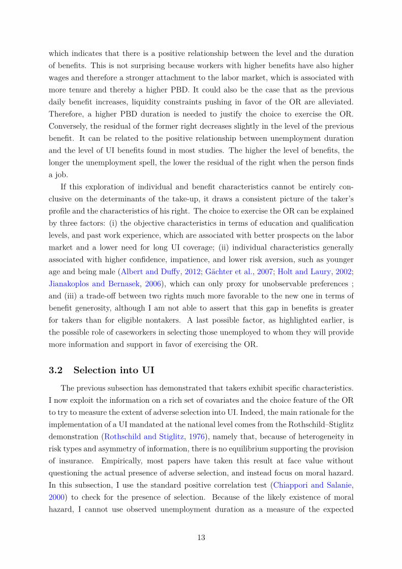
which indicates that there is a positive relationship between the level and the durationof benefits. This is not surprising because workers with higher benefits have also higherwages and therefore a stronger attachment to the labor market, which is associated withmore tenure and thereby a higher PBD. It could also be the case that as the previousdaily benefit increases, liquidity constraints pushing in favor of the OR are alleviated.Therefore, a higher PBD duration is needed to justify the choice to exercise the OR.Conversely, the residual of the former right decreases slightly in the level of the previousbenefit. It can be related to the positive relationship between unemployment durationand the level of UI benefits found in most studies. The higher the level of benefits, thelonger the unemployment spell, the lower the residual of the right when the person findsa job.

If this exploration of individual and benefit characteristics cannot be entirely con-clusive on the determinants of the take-up, it draws a consistent picture of the taker’sprofile and the characteristics of his right. The choice to exercise the OR can be explainedby three factors: (i) the objective characteristics in terms of education and qualificationlevels, and past work experience, which are associated with better prospects on the labormarket and a lower need for long UI coverage; (ii) individual characteristics generallyassociated with higher confidence, impatience, and lower risk aversion, such as youngerage and being male (Albert and Duffy, 2012; Gächter et al., 2007; Holt and Laury, 2002;Jianakoplos and Bernasek, 2006), which can only proxy for unobservable preferences ;and (iii) a trade-off between two rights much more favorable to the new one in terms ofbenefit generosity, although I am not able to assert that this gap in benefits is greaterfor takers than for eligible nontakers. A last possible factor, as highlighted earlier, isthe possible role of caseworkers in selecting those unemployed to whom they will providemore information and support in favor of exercising the OR.

3.2 Selection into UI

The previous subsection has demonstrated that takers exhibit specific characteristics.I now exploit the information on a rich set of covariates and the choice feature of the ORto try to measure the extent of adverse selection into UI. Indeed, the main rationale for theimplementation of a UI mandated at the national level comes from the Rothschild–Stiglitzdemonstration (Rothschild and Stiglitz, 1976), namely that, because of heterogeneity inrisk types and asymmetry of information, there is no equilibrium supporting the provisionof insurance. Empirically, most papers have taken this result at face value withoutquestioning the actual presence of adverse selection, and instead focus on moral hazard.In this subsection, I use the standard positive correlation test (Chiappori and Salanie,2000) to check for the presence of selection. Because of the likely existence of moralhazard, I cannot use observed unemployment duration as a measure of the expected

13

costs to the insured. Unemployment duration is therefore predicted using a sample ofsimilar jobseekers during the two years preceding the implementation of the OR. I usea large set of covariates associated with the worker and his last employer to capture asaccurately as possible all the information that is available to the worker when he hasto decide on his benefit schedule. Different specifications are tested, such as a simpleOLS, a Poisson model to account for the fact that the dependent variable is positive, ormodels for zero-inflated count data. Finally, I implement a machine learning algorithmto avoid making any assumption on the functional form of the relationship betweenunemployment duration and individual and job characteristics. The choice of the modelis based on several goodness-of-fit indicators, such as the root mean squared error. Adetailed discussion of the model is provided in Appendix G.

Table 2 reports the predicted unemployment duration on the sample of interest,namely takers and eligible nontakers under the 20e cutoff. Controls are workers on whichthe prediction model has been trained. The table shows that the predicted unemploymentduration is higher for eligible nontakers than for takers below the 20e threshold. The33-day difference, representing a 13% increase relative to the predicted unemploymentduration of takers, is indicative of significant adverse selection. Jobseekers with higherpredicted unemployment duration are more likely to choose the longest UI coverage. Thesame prediction exercise using a flexible OLS yields lower predicted duration in absoluteterms, but a similar 10% difference between takers and nontakers (Table G2).

While there is a clear and robust difference in predicted unemployment duration be-tween takers and nontakers, pointing to significant adverse selection, potential alternativeinterpretations should be mentioned. First, given that the sample under study is madeof workers with low labor market attachment, it is not unlikely that they are not allinformed about the existence of the OR or fully understand its consequences. This maybe particularly true for low-educated workers for example, who are also likely to exhibit ahigher predicted unemployment risk. If I cannot fully rule out the information channel, Ican check whether the difference in predicted unemployment duration still holds after theOR had been in place for some time. I measure that the difference between takers andnontakers goes in the same direction and is even larger if we focus on workers startingtheir spell at least one year after the implementation of the OR (Table G3 of AppendixG). It is reasonable to think that after one year, workers had time to learn about the ORscheme, especially the ones with the highest unemployment risk who experience frequentunemployment spells and are therefore more familiar with the UI legislation. Second, aspreviously mentioned, there exists anecdotal evidence that caseworkers may influence thedecision of jobseekers, which would therefore change the interpretation of the differencein predicted unemployment risk between takers and nontakers. While there is no registerdata or survey evidence that would allow to quantify and potentially rule out this possi-bility, I can, however, provide some details on the institutional framework. First, there

14

is no particular incentive for the caseworker to make the jobseeker choose one option orthe other. The administrative cost does not differ between both options. The caseworkermay advice some jobseekers that they perceive as riskier to opt for the longest option as itis considered safer. In that sense, the caseworker would use his own private informationto make an insurance choice for the jobseeker. The adverse selection from jobseekerswill therefore be reinforced by the adverse selection coming from caseworkers. Althoughcaseworkers may be better informed about the state of the labor market in a particu-lar region or occupation, this information can be assumed public and available to thejobseeker (possibly at some cost). However, it is reasonable to think that the jobseekerhas private information on his own level of risk that he will not necessarily reveal to thecaseworker.30 Second, according to the law, the initiative of taking up the option rightmust come from the jobseeker himself. These two facts suggest that most of the adverseselection comes from the jobseeker.

The next step of the analysis focuses on the measure of moral hazard using a RDD.

4 The moral hazard cost of UI benefits

4.1 Empirical methodology

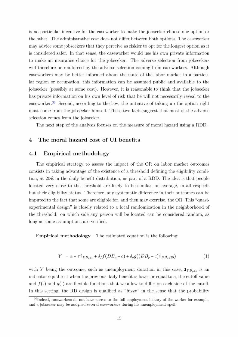
The empirical strategy to assess the impact of the OR on labor market outcomesconsists in taking advantage of the existence of a threshold defining the eligibility condi-tion, at 20e in the daily benefit distribution, as part of a RDD. The idea is that peoplelocated very close to the threshold are likely to be similar, on average, in all respectsbut their eligibility status. Therefore, any systematic difference in their outcomes can beimputed to the fact that some are eligible for, and then may exercise, the OR. This “quasi-experimental design” is closely related to a local randomization in the neighborhood ofthe threshold: on which side any person will be located can be considered random, aslong as some assumptions are verified.

Empirical methodology – The estimated equation is the following:

Y = α + τ1DBp≤c + δff(DBp − c) + δgg((DBp − c)1DBp≤20) (1)

with Y being the outcome, such as unemployment duration in this case, 1DBp≤c is anindicator equal to 1 when the previous daily benefit is lower or equal to c, the cutoff valueand f(.) and g(.) are flexible functions that we allow to differ on each side of the cutoff.In this setting, the RD design is qualified as “fuzzy” in the sense that the probability

30Indeed, caseworkers do not have access to the full employment history of the worker for example,and a jobseeker may be assigned several caseworkers during his unemployment spell.

15

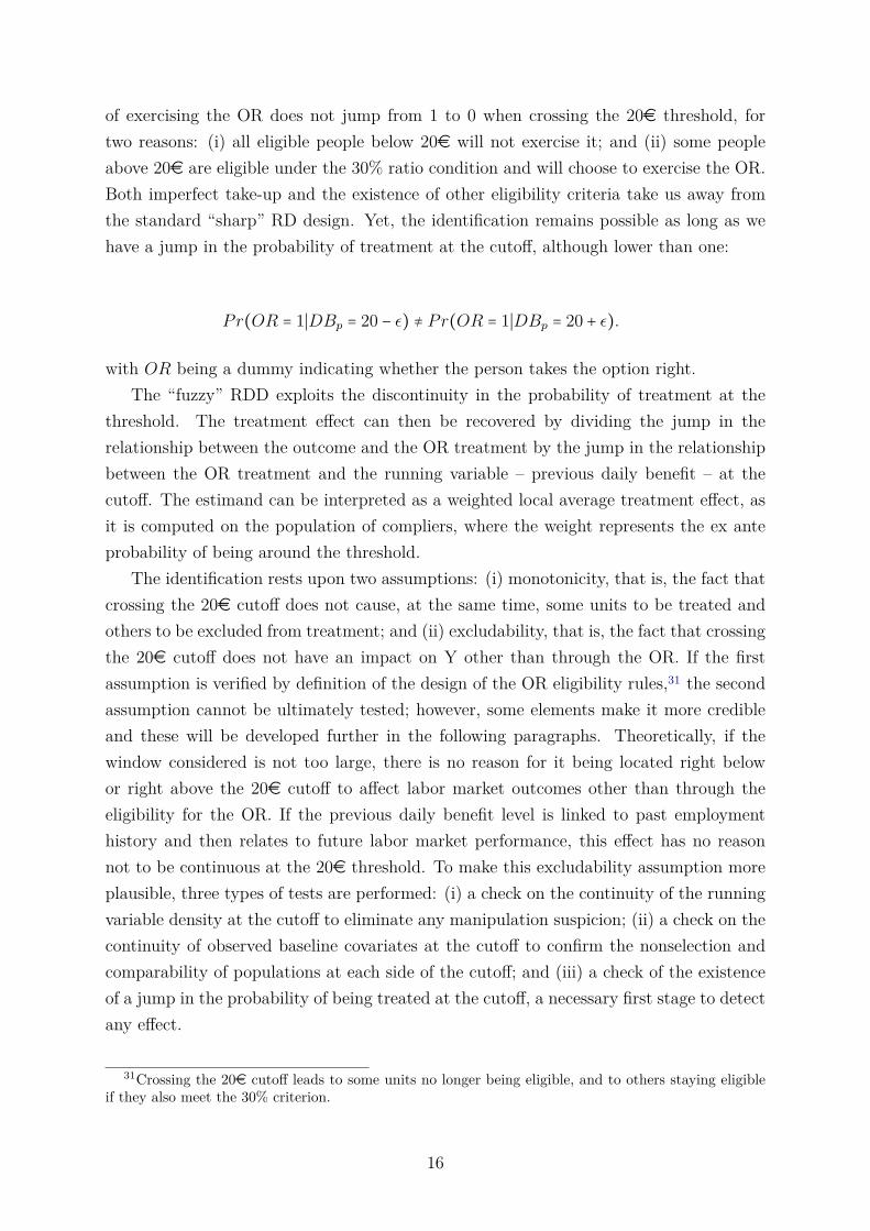
of exercising the OR does not jump from 1 to 0 when crossing the 20e threshold, fortwo reasons: (i) all eligible people below 20e will not exercise it; and (ii) some peopleabove 20e are eligible under the 30% ratio condition and will choose to exercise the OR.Both imperfect take-up and the existence of other eligibility criteria take us away fromthe standard “sharp” RD design. Yet, the identification remains possible as long as wehave a jump in the probability of treatment at the cutoff, although lower than one:

Pr(OR = 1∣DBp = 20 − ε) ≠ Pr(OR = 1∣DBp = 20 + ε).

with OR being a dummy indicating whether the person takes the option right.The “fuzzy” RDD exploits the discontinuity in the probability of treatment at the

threshold. The treatment effect can then be recovered by dividing the jump in therelationship between the outcome and the OR treatment by the jump in the relationshipbetween the OR treatment and the running variable – previous daily benefit – at thecutoff. The estimand can be interpreted as a weighted local average treatment effect, asit is computed on the population of compliers, where the weight represents the ex anteprobability of being around the threshold.

The identification rests upon two assumptions: (i) monotonicity, that is, the fact thatcrossing the 20e cutoff does not cause, at the same time, some units to be treated andothers to be excluded from treatment; and (ii) excludability, that is, the fact that crossingthe 20e cutoff does not have an impact on Y other than through the OR. If the firstassumption is verified by definition of the design of the OR eligibility rules,31 the secondassumption cannot be ultimately tested; however, some elements make it more credibleand these will be developed further in the following paragraphs. Theoretically, if thewindow considered is not too large, there is no reason for it being located right belowor right above the 20e cutoff to affect labor market outcomes other than through theeligibility for the OR. If the previous daily benefit level is linked to past employmenthistory and then relates to future labor market performance, this effect has no reasonnot to be continuous at the 20e threshold. To make this excludability assumption moreplausible, three types of tests are performed: (i) a check on the continuity of the runningvariable density at the cutoff to eliminate any manipulation suspicion; (ii) a check on thecontinuity of observed baseline covariates at the cutoff to confirm the nonselection andcomparability of populations at each side of the cutoff; and (iii) a check of the existenceof a jump in the probability of being treated at the cutoff, a necessary first stage to detectany effect.

31Crossing the 20e cutoff leads to some units no longer being eligible, and to others staying eligibleif they also meet the 30% criterion.

16

Validity conditions of the RDD – One key assumption to check for the RDD tobe valid is that there is no manipulation at the threshold, or strategic sorting of workersat either side of the threshold. Theoretically, there are several reasons why unemployedpeople would not have an interest in reporting lower earnings to have a DB just belowthe 20e cutoff: (i) they would receive very low benefits, lower than they were entitled toif they had reported their true earnings; (ii) the earnings value used to compute DB isreported on a certificate delivered by the employer to open UI rights, making falsificationvery unlikely; and (iii) manipulating their earnings value in anticipation of a future ORwould require very accurate foresight, as well as a precise knowledge of UI legislation.32

Although the manipulation scenario seems implausible, I still perform a McCrary test(McCrary, 2008) to check that the density of the former DB distribution is smooth at the20e cutoff (Figure C1). Some regularities in the level of earnings or in the UI parameterstend to create small spikes at different points of the distributions, without threateningthe validity of the RDD, as these spikes are not in the neighborhood of the cutoff. Forexample, we observe a big jump in density around 32e, as this corresponds to the levelof DB for a person who has worked full-time at the minimum wage. As there is noprecise sorting at the threshold, RDD is considered “as good as randomization” in theneighborhood of the threshold.

If I chose to focus on one eligibility criterion for data limitation issues, it would still bepossible to observe which eligibility criterion was binding for eligible workers who choseto exercise the OR. The distribution across eligibility conditions for takers shows thatthe most decisive criterion is having a new daily benefit greater than the former one byat least 30%. Indeed, 97.5% of takers having a previous DB lower than 20e also fulfillthe ratio criterion, and 92.2% of all takers fulfill the ratio criterion (Table E1). Thisdistribution emphasizes the fact that having information on both criteria would havehelped to capture the OR impact in a more exhaustive way and that the populationof compliers is very specific, being made up of people eligible under the 20e criterionbut not under the 30% criterion. Indeed, the share of people eligible based on the 30%criterion have no reason not to be continuous at the 20e threshold,33 meaning thatthe compliers have a financial gain when exercising the OR necessarily lower than 30%,translating into at most 6e daily. This implies that compliers are willing to give up ona significant additional coverage duration (336 days on average) for a limited increase inincome, demonstrating either particular preferences, very tight financial constraints, or

32It would require unemployed people to be aware of the existence of the OR, to anticipate that theywill find a job and lose it again, and then that they might be eligible, and to know very precisely therules to compute DB from earnings, with some parameters being updated every semester.

33I cannot ultimately test this as I cannot identify the eligible population, but the continuity assump-tion at least holds for the percentage of takers under the 30% criterion. This alleviates the suspicionthat take-up could be discontinuous at the threshold also because of people already eligible under the30% criterion, who exercise the OR, but who would not have exercised it if they had been above thethreshold because of higher salience of the OR possibility under the threshold.

17

very optimistic anticipation about their return to the labor market.To conclude fully that the difference in outcomes we observe between populations

at each side of the threshold can be imputed to differences in OR take-up, we need torule out the influence of other variables at the threshold. Appendix H displays differenttests of the continuity of covariates at the threshold. Figures H1–H7 do not depict anyclear jump in the distribution of covariates at the threshold, and the whole distributionpattern shows numerous bumps and lumps at other values of the covariates. In addition,Figure C2 (Appendix C) provides the corresponding RD estimates, where each covariateis used as the dependent variable in the RD regression, and previous daily benefit as therunning variable. None of the coefficient is significantly different from zero, except forthe tenure at past job. Although strategic sorting of people on either side of the thresh-old is very unlikely,34 I also test the continuity of the predicted unemployment duration,which can be considered an index of various characteristics. Unemployment duration ispredicted using a sample of similar workers unemployed during the two years preced-ing the introduction of the option right, and performing an out-of-sample prediction onthe sample under study. Included variables are age, gender, skill level (5 categories),education level (10 categories), sought occupation (14 categories), part-time coefficient,region of residence (31 categories), sector of activity (11 categories), month of contracttermination, number of children, family situation (5 categories), previous occupation (81categories), firm and plant size. A flexible linear model is used, yielding a R2 equal to7% and a RMSE equal to 281. The rather low R2 can be explained by the fact that Ido not include any variable related to the UI entitlements, because these variables mayinterfere with the effect of the option right itself. Figure H8 (Appendix H) shows nodiscontinuity in the distribution of predicted unemployment duration at the eligibilitythreshold. Further, Table C1 reports the RD estimates without controls, controlling forpredetermined variables (age, gender, level of education) and controlling for the value ofpredicted unemployment. Although coefficients move a bit, they are qualitatively similarand do not alter the conclusion that the option right significantly increases paid unem-ployment duration.

First-stage estimation – Empirically, I estimate Equation 1 nonparametrically us-ing a restricted window around the threshold. To demonstrate the robustness of theeffect, results will be shown for a range of different polynomial orders and bandwidthsizes.35 Equation 1 shows the reduced form of two equations capturing the first-stage

34Sorting would imply that workers anticipate, when opening their UI right, that they might exercisethe OR in the future if they work in a better paid job (in some cases even before the OR has beenimplemented), and, in order to be eligible, they should be willing to falsify their work certificate toreceive lower benefits immediately

35Table I1 and Figure D1 of Appendices D and I reproduce the main results making the size of thebandwidth vary (choosing, in particular, between 0.5 and 3 times the optimal bandwidth value).

18

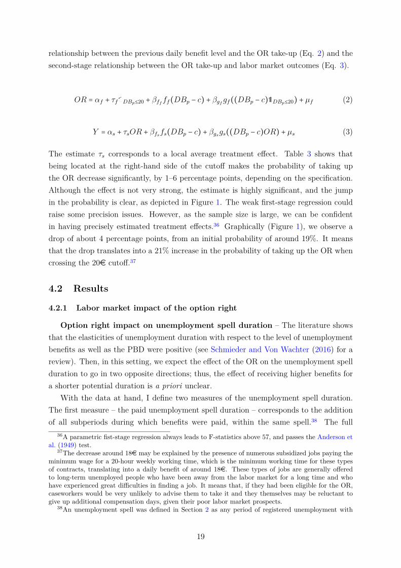
relationship between the previous daily benefit level and the OR take-up (Eq. 2) and thesecond-stage relationship between the OR take-up and labor market outcomes (Eq. 3).

OR = αf + τf1DBp≤20 + βffff(DBp − c) + βgf

gf((DBp − c)1DBp≤20) + µf (2)

Y = αs + τsOR + βfsfs(DBp − c) + βgsgs((DBp − c)OR) + µs (3)

The estimate τs corresponds to a local average treatment effect. Table 3 shows thatbeing located at the right-hand side of the cutoff makes the probability of taking upthe OR decrease significantly, by 1–6 percentage points, depending on the specification.Although the effect is not very strong, the estimate is highly significant, and the jumpin the probability is clear, as depicted in Figure 1. The weak first-stage regression couldraise some precision issues. However, as the sample size is large, we can be confidentin having precisely estimated treatment effects.36 Graphically (Figure 1), we observe adrop of about 4 percentage points, from an initial probability of around 19%. It meansthat the drop translates into a 21% increase in the probability of taking up the OR whencrossing the 20e cutoff.37

4.2 Results

4.2.1 Labor market impact of the option right

Option right impact on unemployment spell duration – The literature showsthat the elasticities of unemployment duration with respect to the level of unemploymentbenefits as well as the PBD were positive (see Schmieder and Von Wachter (2016) for areview). Then, in this setting, we expect the effect of the OR on the unemployment spellduration to go in two opposite directions; thus, the effect of receiving higher benefits fora shorter potential duration is a priori unclear.

With the data at hand, I define two measures of the unemployment spell duration.The first measure – the paid unemployment spell duration – corresponds to the additionof all subperiods during which benefits were paid, within the same spell.38 The full

36A parametric fist-stage regression always leads to F-statistics above 57, and passes the Anderson etal. (1949) test.

37The decrease around 18e may be explained by the presence of numerous subsidized jobs paying theminimum wage for a 20-hour weekly working time, which is the minimum working time for these typesof contracts, translating into a daily benefit of around 18e. These types of jobs are generally offeredto long-term unemployed people who have been away from the labor market for a long time and whohave experienced great difficulties in finding a job. It means that, if they had been eligible for the OR,caseworkers would be very unlikely to advise them to take it and they themselves may be reluctant togive up additional compensation days, given their poor labor market prospects.

38An unemployment spell was defined in Section 2 as any period of registered unemployment with

19

unemployment spell duration corresponds to all registered subperiods within the samespell, including the unpaid ones, which, by definition of the spell, last less than 4 months.It allows to include days when jobseekers have potentially exhausted their benefits butstay registered. However, restricting the analysis to the unemployment spell duration maysometimes not be relevant; if the person keeps going back and forth, in and out of thelabor market, the unemployment spell may be short without necessarily correspondingto a stable exit from the labor market.39 That is why this measure will be presentedwith other complementary outcome variables intended to capture a medium- to long-term effect. Tables 4 and 5 show that taking up the OR has a strong and significanteffect on unemployment spell duration – both paid and unpaid. If we focus on thequadratic specification without any controls of Table 4, the OR leads to an increasein paid unemployment duration of about 157 days. The effect is markedly large, andthe OR seems to have a very detrimental impact on the employment outcomes of apopulation already in a precarious situation. In particular, if we consider that the averageduration of a spell at the cutoff is around 92 days, the effect is equivalent to multiplyingthe spell duration by 2.7.40 At first sight, evidence would lead to the conclusion thatletting the unemployed choose the terms and conditions of their compensation is a veryinefficient way of ensuring satisfactory coverage and a quick return to the labor market.The strong and positive effect on unemployment duration is confirmed by Figures 2 and3. The addition of covariates does not change the order of magnitude of the results forany specification, which is reassuring on the validity of the RDD. The results are alsovery consistent across the local linear and quadratic polynomials. Tables D1 and D2 ofAppendix D report the reduced-form coefficients, which range from 7 to 8 days for thepaid unemployment duration, and 11 to 16 days for the full unemployment duration.For both outcome variables, it represents about a 10% increase relative to the controloutcome mean, and coefficients are remarkably stable across specifications.

These different findings indicate that benefiting from a shorter potential durationwith a higher average level of benefits and a declining profile makes the duration of theunemployment spell increase. In this specific context, the elasticity of unemploymentduration to the level of unemployment benefits outweighs the elasticity of unemploymentduration with respect to the PBD. This result is in line with the literature, as elasticitiesof nonemployment duration or benefit duration with respect to the benefit level areusually higher than the same elasticities measured with respect to PBD (see Schmieder

interruptions shorter than 4 months. Then, the paid unemployment spell duration refers to the additionof registered and paid subperiods without counting the time elapsed during the interruptions.

39Nevertheless, as unemployment spells are defined so that they are separated by at least 4 monthsof interruption, we can be fairly confident that the end of an unemployment spell corresponds to a jobof at least several months.

40It should be noted that the control outcome mean refers to the mean paid unemployment spellduration for values of the DB right above the cutoff, between 20e and 30e, but the counterfactualaverage duration of the spell for compliers in the absence of the OR may differ.

20

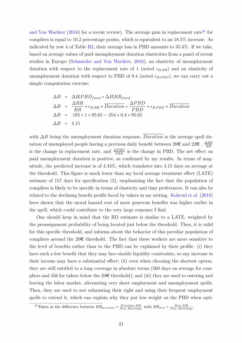
and Von Wachter (2016) for a recent review). The average gain in replacement rate41 forcompliers is equal to 10.2 percentage points, which is equivalent to an 18.5% increase. Asindicated by row 4 of Table B2, their average loss in PBD amounts to 35.4%. If we take,based on average values of paid unemployment duration elasticities from a panel of recentstudies in Europe (Schmieder and Von Wachter, 2016), an elasticity of unemploymentduration with respect to the replacement rate of 1 (noted εB,RR) and an elasticity ofunemployment duration with respect to PBD of 0.4 (noted εB,P BD), we can carry out asimple computation exercise:

∆B = ∆B∣PBDfixed +∆B∣RRfixed

∆B = ∆RRRR

× εB,RR ×Duration + ∆PBDPBD

× εB,P BD ×Duration∆B = .185 × 1 × 95.65 − .354 × 0.4 × 95.65

∆B = 4.15

with ∆B being the unemployment duration response, Duration is the average spell du-ration of unemployed people having a previous daily benefit between 20e and 22e , ∆RR

RR

is the change in replacement rate, and ∆P BDP BD is the change in PBD. The net effect on

paid unemployment duration is positive, as confirmed by my results. In terms of mag-nitude, the predicted increase is of 4.34%, which translates into 4.15 days on average atthe threshold. This figure is much lower than my local average treatment effect (LATE)estimate of 157 days for specification (2), emphasizing the fact that the population ofcompliers is likely to be specific in terms of elasticity and time preferences. It can also berelated to the declining benefit profile faced by takers in my setting. Kolsrud et al. (2018)have shown that the moral hazard cost of more generous benefits was higher earlier inthe spell, which could contribute to the very large response I find.

One should keep in mind that the RD estimate is similar to a LATE, weighted bythe preassignment probability of being located just below the threshold. Then, it is validfor this specific threshold, and informs about the behavior of this peculiar population ofcompliers around the 20e threshold. The fact that these workers are more sensitive tothe level of benefits rather than to the PBD can be explained by their profile: (i) theyhave such a low benefit that they may face sizable liquidity constraints, so any increase intheir income may have a substantial effect; (ii) even when choosing the shortest option,they are still entitled to a long coverage in absolute terms (560 days on average for com-pliers and 456 for takers below the 20e threshold); and (iii) they are used to entering andleaving the labor market, alternating very short employment and unemployment spells.Then, they are used to not exhausting their right and using their frequent employmentspells to extend it, which can explain why they put less weight on the PBD when opti-

41Taken as the difference between RRprevious =P revious DB

New Earningswith RRnew =

New DBNew Earnings

.

21

mizing their search behavior. (iv) Finally, the population on which the effect is measuredhas self-selected into the treatment, implying that they are likely to react more than inother settings found in the literature where no choice is involved.

Longer-term impact on the professional path – Looking only at this first evi-dence on unemployment duration would lead one to conclude that the OR has a negativeimpact on employment. However, the ultimate impact on a worker’s welfare dependson whether this increase in the duration of the subsequent unemployment is driven bythe fact that the person can afford to take more time to find a job, and that this jobwill be more stable and of better quality. Even though job quality cannot be measureddirectly with the available data, because I have no information on the job found whenthe unemployed person leaves the rolls, we can still try to capture a longer-run effect,by measuring the total number of days spent unemployed after the exercise of the OR.If the OR was associated with an increase in job quality, we would observe that, despitea longer immediate unemployment spell, people exercising the OR would be less unem-ployed over the whole subsequent period. I now define two new outcome variables: thetotal number of days unemployed over the subsequent period, and the total number ofdays on UI benefits over the subsequent period. Figures I1 and I2 (Appendix I) exhibita drop in the total number of days registered as unemployed over the subsequent period,but not in the total number of days on UI benefits over the subsequent period. Con-sequently, Tables 6 and 7 show that the effect on the total number of days registeredas unemployed is significant for all specifications, whereas it is never significant for thetotal number of days on benefits. The total number of days unemployed is measured ontime periods of different lengths depending on the starting date of the spell. This shouldnot be an issue to the extent that the starting date of the spell is uniformly distributedacross treated and controls. Figures E2 and E3 are reassuring on this issue.42 However,I provide the results on the total number of days unemployed over a two and three-yearperiod (Table I6 of Appendix I). Results are less precise due to the small sample size:they point to a positive to nonsignificant effect of the OR on the longer-run number ofdays unemployed. This is confirmed by the graphical evidence displayed on Figures I4and I3. If anything, the effect would be positive on the total number of days registeredas unemployed, consistent with Tables 6 and 7.

Several interpretations of this difference between the effect on the total number of dayson benefits and the total number of days registered as unemployed can be put forward.Being registered as unemployed without receiving benefits generally corresponds to either

42Figure E2 shows that the distribution of the starting date of the spell is rather uniform across groupsof workers with the former benefit above and below the 20e cutoff. Figure E3 further shows that theprobability to fall under the 20ethreshold is rather stable over time. The difference in entry date, if any,would rather lead to underestimating the results in terms of unemployment duration as those earningmore than 20e enter more frequently at the beginning of the period.

22

(i) periods during which the unemployed receives assistance benefits, or (ii) periods duringwhich the person works while registered as unemployed, because he is still looking foranother job or because his contract is short. I examine the plausibility of each motivein the following paragraphs. Distinguishing between both explanations is a key issue.The first scenario would mean that the higher number of days registered as unemployedbut not paid corresponds to unemployed people at the exhaustion point of their right,staying registered to keep benefiting from the support of the caseworker. In particular,to receive assistance benefits or the minimum income, it is required to be registeredas unemployed. This would be compatible with the fact that takers have mechanicallyshorter PBD than nontakers. It would mean that evidence in Tables 6 and 7 and Figure I1supports the hypothesis that the OR slows down the return to work, even in the longrun, and forces takers to switch to assistance benefits as they are no longer entitled toUI benefits. If the second scenario prevails, it implies that, in the long run, takers workslightly more, although it can be under temporary and part-time contracts. My data donot contain, at the moment, information on assistance benefits,43 but the data can stillinclude jobseekers staying registered without receiving any income from UI, after theyexhausted their benefits for instance. Table 8 indicates that compliers are more likely toreach the exhaustion point of their benefits by 13–17 percentage points depending on thespecification, from a baseline of around 4% (Figure 4). Then, the difference we observein terms of number of days registered could be partly explained by the fact that takersrun out of benefits more frequently.44

The second motive may more plausibly explain the main difference in the numberof days registered but not paid. Anecdotal evidence has revealed that caseworkers wereadvising unemployed people who found a job under a fixed-term contract to maintainregistration at the job center to avoid starting the whole procedure again at the end oftheir contract. It is also particularly recommended when the job is temporary, part-time,or corresponds to qualifications that do not perfectly match those of the worker, so thatthe person can keep looking for a better job and benefiting from support and guidancefrom the caseworkers. Therefore, if we believe that the higher number of days registeredbut not paid corresponds to trial periods at the beginning of an open-ended contract,when the worker is not sure yet of being permanently hired, we may consider that theOR acts as a stepping-stone to a more stable job in the long run. Another reason peoplewould stay registered as unemployed while working is that they earn a sufficiently lowwage to be entitled to receive complementary benefits from UI. The benefits received arelower than a full month of complete compensation, and the person would then appear asbeing on benefits for some days in the month and registered but not receiving benefits

43Assistance benefits such as the minimum income are managed by another administration.44Indeed, if I do not observe jobseekers receiving the minimum income for example,

23

for the rest of the month.45 In other words, these periods during which the person isregistered without receiving benefits generally correspond to employment spells underunstable, temporary, and/or part-time contracts. For example, if, in a given month, theperson is employed under a part-time contract and is entitled to receive one-third of themonthly benefits he would receive with no job at all, he will appear as registered onbenefits for 10 days in the month, and registered without benefits for the other 20 days.However, if the person has no job at all, he will appear as registered on benefits for all30 days. This scenario is then compatible with takers having a similar total number ofdays on UI benefits with a higher total number of days registered without benefits at thesame time. Overall, the evidence suggests that in the medium to long run, the OR doesnot impact negatively on the professional path in terms of unemployment probability,although it may encourage temporary, unstable, and part-time contracts.

The next subsection investigates in greater detail whether the difference in terms ofdays registered as unemployed can be explained by takers having more frequent smallemployment spells while maintaining registration.

Impact on partial employment – If an unemployed person works while registeredas unemployed, I am able to track the employment spells and to have information onthe number of hours worked and total earnings, no matter whether still earning benefitsduring this period. These types of employment spells typically include short-term andpart-time contracts rather than a stable job.46 In the remainder of the paper, I will referto these periods of employment while registered as unemployed as partial employment.I observe that people exercising the OR have a probability of experiencing partial em-ployment during the unemployment spell that is much higher than the control group(Table 9).47 This finding is consistent with the fact that the impact I measure on unem-ployment duration is higher in terms of number of days registered than in the number ofdays receiving benefits, both in the short and long term. The fact that compliers earnmore income from labor during the spell (Table I3 of Appendix I), conditional on workingat least 1 hour during the spell, is presumably explained by more hours worked (Table I4of Appendix I). I also measure the unconditional impact of the OR on hourly wage earnedwhile registered as unemployed. This impact is unbiased as it is not conditional on work-ing during the UI spell, which is endogenous, but does not allow us to separate the impacton the probability of work from the intensive margin impact. Table D4 of Appendix Dshow nonsignificant results, suggesting that, given the positive impact on the probability

45Jobseekers are entitled to receive benefits as long as the sum of their labor income and their UIbenefits does not exceed their previous earnings.

46Survey evidence (Unédic, 2018) shows that 70% of individuals working while on UI benefits areunder a fixed-term contract.

47The RD estimation yields estimates larger than one because it does not account for the binarynature of the variable. A parametric estimation using bivariate probit indicates a 55 pp increase in theprobability to work during the UI spell caused by the option right (Table D3 of Appendix D).

24

to work during the UI spell, there is no positive impact of the OR on hourly wage.48 Al-though compliers resort more often to partial employment during the UI spell, the typeof job they find is not of better quality, if we assume that the wage rate is a good proxyfor job quality.

Taken together, these findings suggest that people exercising the OR are not only onbenefits for a longer time in the short run, but also experience a more unstable path,alternating frequently between short periods of employment and unemployment. It couldalso be the case that people accustomed to partial employment are less worried abouthaving a shorter unemployment right and focus more on the generosity of UI benefits, asthey know they will find short-term employment contracts to extend the length of theirUI entitlements.49

4.2.2 The optimization ability of the unemployed

Because the impact of the OR on unemployment duration is markedly negative in theshort run, and less clear in the long run, the ultimate welfare impact is not straightfor-ward. The presence of adverse selection discussed in section 3.2 suggests that jobseekershave a significant amount of private information about their unemployment risk. If thatis the case, they should be able to choose the option that optimizes their compensationbased on this information. Answering the question of whether the unemployed made theright decision is complex, and made difficult by the lack of data on the full set of insurancecontracts for eligible nontakers. However, I explore several outcomes that shed light atthe link between the OR and the welfare and optimization ability of jobseekers. A firstdimension relates to the comparison of total income earned by compliers and controls,and a second one relates to the risk of ending up with no income at all.

I start investigating the first dimension by measuring the effect of OR on daily earn-ings, defined as the sum of UI benefits and earnings from work divided by the durationof the unemployment spell.50 It allows to account both for the fact that earning morebenefits or wage presumably increases welfare, whereas having a longer UI spell maydecrease welfare. Table I5 (Appendix I) indicates a negative impact on daily earnings,suggesting that the effect of OR on unemployment duration outweighs the effect of ORon the total amount of benefits and the probability to work while unemployed.51

48RD estimates on the conditional hourly wage are negative and nonsignificant. Tables are availableupon request.

49A descriptive analysis of individuals working while being on UI benefits (Unédic, 2016) revealsthat their profile is quite consistent with that of compliers: more frequently female, and working in thepersonal care sector.

50I do not use any time discount factor in this analysis.51It should be again emphasized that earnings from work are only observed if the person stays reg-

istered as unemployed. Although it is a limitation, since daily earnings are measured during the unem-ployment spell, taking a job implies in most cases staying registered as unemployed, and working onlyfor short spells. Given the results on the probability of working while unemployed, and the fact thatestimates on daily earnings are negative, it suggests that, if anything, the effect is underestimated.

25

A second important outcome to take into account is whether takers reach the exhaus-tion point of their entitlements. Indeed, if by exercising the OR they lose benefit duration,they could still be entitled to a longer coverage. If they are not at risk of running outof benefits, taking up the OR would simply mean having higher benefits, and would bea risk-free way to maximize benefits collected. Table I2 of Appendix I shows that in-deed only a small percentage of takers, 17%, exhaust their UI entitlement. However, thestrong effect of the OR on the probability of exhausting benefits (+15 percentage points,Table 4) suggests that at least a portion of the unemployed choosing the OR becausethey anticipate a quick return to the labor market fail in their prediction.

To have a sense of whether some groups of unemployed are better optimizers relativeto others, I perform a heterogeneity analysis, intersecting the propensity to take the ORwith the outcome in terms of unemployment spell duration. The idea is to analyze whichsubpopulations are more likely to take the OR, and whether they experience a negativeimpact on their employment prospects by doing so. Using age, gender, and educationcategories and comparing the first and second stage for each category, I observe thatyounger unemployed people have a higher jump in the probability of taking up the ORat the 20e threshold (Table D5 of Appendix D), which is compatible with the less stableprofessional status that is often experienced in the early years of the career. Youngerworkers (under 35 years old) do not optimize perfectly, because both their take-up andthe negative impact on unemployment duration are of high magnitude. Older workershave insignificant first- and second-stage estimates. Some exercise the OR but they donot seem to resort to it under the 20e criterion. Similarly, Table D5 points to a hightake-up jump for people with a higher level of education, with a limited negative impactfor the very top of the distribution. In particular, we observe that people with highereducation display a significant and substantial jump in take-up while the impact onunemployment duration is lower than the average, whereas it is negative and of highermagnitude for people who only completed high school, despite a higher first stage. Inline with this result on education, we observe that unskilled employees and workers oftenexercise the OR whereas the impact is markedly negative for them. On the contrary,the skilled worker and executive categories are where the jump in take-up is highestwith a limited or insignificant effect on unemployment duration. This means that theirqualifications play a role in protecting them from the adverse impact of the OR on labormarket performance. The OR is also more detrimental to men, because they exhibit ahigher discontinuity in take-up, coupled with a similar negative impact on labor marketoutcomes than women.

Overall, it seems that workers in the middle and the top of the age and skills distri-bution, as well as the highly educated, are those gaining the most advantage from theOR, with a limited impact on their subsequent unemployment spell duration. One inter-pretation is that they are better at predicting their reemployment probability, and that

26

they have at the same time better objective labor market prospects. Better educatedworkers are more likely to take the risk of exercising the OR without increasing theirunemployment spell duration too much, because they are better equipped to find a jobrapidly and they may have a more stable professional status. However, it is also possiblethat different subgroups face different treatment intensity: for example, young peopleare likely to experience an erratic earnings trajectory in the beginning of their career,with substantial jumps in income from one job to the other. Therefore, the differencein benefit between both options may be larger than for other categories. Their higherpropensity to take the OR could then be rationalized by a different treatment inten-sity, keeping preferences and employment prospects equal. I cannot observe the full setof insurance contracts offered to different subgroups, but only those offered to takers.52

Based on this information, I regress the ratio of benefits and the ratio of PBD in caseof takeup relative to nontakeup on a number of observable characteristics.53 Youngerand more skilled takers have, on average, a higher PBD ratio but a lower benefit one,making the net effect on treatment intensity ambiguous. Level of education, is, however,negatively correlated with both ratios. It means that highly-educated workers have ahigher propensity to take the OR despite the fact that we observe that highly-educatedworkers gain less by taking the OR than the average of other takers. It suggests that,assuming they have the same preferences than the average worker, they anticipate a quickreturn to the labor market. The fact that they experience only a limited increase in theirunemployment duration, however, can be explained both by less intensive treatment orbetter employment prospects.

4.3 Adverse selection and moral hazard

The correlation between observed unemployment duration and the OR take-up mixesmoral hazard and adverse selection. The challenge of the analysis is to disentangle thetwo, and to compare their magnitude. Table 2 points to the existence of significant adverseselection in this setting. This is confirmed by Tables 10 and 11 where the population isdivided into quintiles of predicted unemployment duration. Table 10 focuses on thesubsample of workers with previous daily benefit lower than 20e, where we can preciselyidentify the population of eligibles. On this sample, we observe that the take-up rateis a decreasing function of the predicted unemployment duration, except for the fourthquintile, which means that the higher the unemployment risk, the more likely it is thatthe worker will choose the longest coverage. Consistently, Table 11 shows, on the wholesample, that the jump in take-up at the threshold is the highest in the lowest quintiles.

52The information on the options faced by takers does not allow to fully conclude on the potentialheterogenous treatment intensity, because it is conditional to the endogenous takeup decision. However,it is still informative on the expectations of different subgroups of takers.

53Tables are available upon request.

27

For both tests, the pattern in the middle of the distribution is less clear. However,they indicate that the bottom of the predicted unemployment duration is systematicallyassociated with a higher takeup, whereas the top of the distribution is systematicallyassociated with a lower takeup. This correlation test with the predicted unemploymentduration, although it may not capture the role of unobservables, is indicative of adverseselection.

We know from the previous section that the moral hazard response to the OR is sub-stantial, as measured by the increase in the unemployment spell duration at the eligibilitythreshold. I try to go further by analyzing the response on the different predicted unem-ployment duration quintiles (Table 12). It shows that, as the predicted unemploymentduration increases, the negative impact of the OR also increases, meaning that those whoare initially predicted to stay unemployed longer will suffer even more from choosing ashorter coverage with higher benefits. Although, here again, the relationship is less clearin the middle of the distribution, we observe that workers in the top quintile of predictedunemployment duration suffer from a negative impact of the option right on their em-ployment prospects three times larger than workers in the bottom quintile. These resultssuggest that the policy designed to give a certain degree of flexibility in the UI choice iswidening inequalities in terms of employment probability.

Following ?, I use the following decomposition to separate moral hazard (MH) fromadverse selection (AS).

ES[π∣Short] −EL[π∣Long] = ES[π∣Short] −ES[π∣Long]´¹¹¹¹¹¹¹¹¹¹¹¹¹¹¹¹¹¹¹¹¹¹¹¹¹¹¹¹¹¹¹¹¹¹¹¹¹¹¹¹¹¹¹¹¹¹¹¹¹¹¹¹¹¹¹¹¹¹¹¹¹¹¹¹¹¹¹¹¹¹¹¹¹¹¹¹¹¹¹¹¹¹¹¹¸¹¹¹¹¹¹¹¹¹¹¹¹¹¹¹¹¹¹¹¹¹¹¹¹¹¹¹¹¹¹¹¹¹¹¹¹¹¹¹¹¹¹¹¹¹¹¹¹¹¹¹¹¹¹¹¹¹¹¹¹¹¹¹¹¹¹¹¹¹¹¹¹¹¹¹¹¹¹¹¹¹¹¹¹¹¶MH

+ES[π∣Long] −EL[π∣Long]´¹¹¹¹¹¹¹¹¹¹¹¹¹¹¹¹¹¹¹¹¹¹¹¹¹¹¹¹¹¹¹¹¹¹¹¹¹¹¹¹¹¹¹¹¹¹¹¹¹¹¹¹¹¹¹¹¹¹¹¹¹¹¹¹¹¹¹¹¹¹¹¹¹¹¹¹¹¹¹¹¹¹¸¹¹¹¹¹¹¹¹¹¹¹¹¹¹¹¹¹¹¹¹¹¹¹¹¹¹¹¹¹¹¹¹¹¹¹¹¹¹¹¹¹¹¹¹¹¹¹¹¹¹¹¹¹¹¹¹¹¹¹¹¹¹¹¹¹¹¹¹¹¹¹¹¹¹¹¹¹¹¹¹¹¹¶AS

AS = Observed difference −RDD estimate

= 79 − 157

= −78

∣AS∣ ≈ 50% MH

The change in unemployment duration between people randomly offered the choice of theshort option versus a situation in which everyone is assigned to the long option is measuredby the RDD coefficient, and captures the moral hazard cost.54 The observed differenceis measured as the difference between takers and nontakers under the 20e cutoff. Thechoice to restrict to this subsample is justified by the fact that the adverse selectionmeasured in Table 2 is computed on the same sample, as it is the only population where

54The moral hazard estimate goes in the opposite direction to what is usually found. This counter-intuitive result is actually explained by the fact that it measures a combination of a change in the overallamount of UI benefits as well as a change in the benefit profile. The estimate captures the effect ofreceiving higher benefits in the short-run and lower benefit in the long-run compared to the oppositeprofile. It therefore suggests that the moral hazard cost is higher in the beginning of the spell, endingup in a positive net effect of the OR on unemployment spell duration.

28

I can assess the eligibility criteria even for nontakers. Because I want to measure therelationship between unemployment risk and insurance contract decision, I want to ensurethat nontakeup is not actually explained by noneligibility. In addition, the moral hazardcost is estimated on the population of compliers, who are workers meeting the 20e butnot the 30% condition. I cannot measure the observed difference on the same population,by comparing the observed unemployment duration of compliers and nontakers meetingthe 20e but not the 30% condition, because I do not observe this last condition onnontakers. However, restricting to the sample below 20e allows to get closer to thesample where I measure moral hazard. Reassuringly, the observed difference betweentakers and nontakers above the 20e cutoff is also equal to 79 days. Adverse selectionis retrieved from the subtraction of moral hazard from the observed difference in theunemployment spell duration between people choosing the long and the short options.The figures used are based on the duration of the paid unemployment spell immediatelyfollowing choosing whether to exercise the OR. This computation suggests that, althoughadverse selection is sizable, moral hazard is far more substantial in this setting.

4.4 Robustness tests

Definition of the unemployment spell – The preferred definition of the unemploy-ment spell used throughout the paper is the gathering of days registered as unemployedwithout any interruption of at least 4 months. The 4-month criterion has been chosento ensure that the interruption reflects a stable return to work, and because it is theminimum working requirement to be able to open a new UI right. The definition chosenshould not affect the result to the extent that we are comparing people at the direct neigh-borhood of the 20e cutoff. Nonetheless, it could be argued that if people exerting the ORare more prone to experience very short employment spells while still being registered asunemployed, it could inflate the duration of the unemployment spell as defined earlier,even though these small employment periods are not counted in the unemployment spellduration. To alleviate this concern, I perform the same analysis on the duration of thespell before an interruption in payment of different durations (from 1 day to 2 months).Table D6 of Appendix D exhibits very similar reduced-form estimates when expressedrelative to the average duration of the spell (the last two columns reproduce the mainspecification). Then, the measured impact on unemployment spell duration does notdepend on the definition of the spell I choose to adopt. I also reproduce the main resultslooking at the probability of being unemployed at different time horizons (Tables I7, I8of Appendix I). These findings confirm that the main effect on employment probabilityoccurs in the short term, more precisely within a 9-month horizon.

Permutation test – I perform a nonparametric permutation test in the same spirit

29

of Chetty et al. (2009) where RD estimates are computed for 1,000 randomly chosenvalues of the cutoff. Defining F (β̄p) to be the empirical cumulative distribution functionof these placebo effects, the statistic F (β) gives a p-value for the hypothesis that β = 0.Intuitively, if the option right had a significant effect on unemployment duration, wewould expect the estimated reduced-form coefficient to be in the lower tail of estimatedplacebo effects. Figure I5 (Appendix I) reports the cumulative distribution function ofthe RD estimate for paid unemployment spell duration measured using these placebovalues. The solid vertical line denotes the treatment effect on the real cutoff, which liesoutside the 95% confidence interval (dashed lines). I obtain F (β) = 0.04. The p-value islarger than the one obtained using t-test, but it confirms that the option right has a truepositive effect on unemployment duration.55

5 Concluding remarks

This paper takes advantage of an uncommon setting in which unemployed people areoffered a choice between two unemployment benefits schedules. It is a priori unclearwhat makes the worker better-off between receiving on average higher benefits for ashorter duration or having a longer PBD with lower average benefits. This paper looksprecisely at the combined effect of a variation in the level, duration and profile of benefitson labor market outcomes. Opting for the short and high-benefit schedule increasesdramatically the length of the subsequent unemployment spell. This finding suggeststhat the moral hazard cost of UI benefits is larger early in the spell. This effect isparticularly worrying if we consider that the targeted population is already at risk in thelabor market, alternating unemployment and employment spells. However, the effect isno longer significant when considering a longer time horizon: the unemployed choosingthe short and high-benefit schedule do not experience more days on UI benefits over thewhole of the following period, but they resort more to short-term and part-time workcontracts. The main mechanism explaining both the divergence between the short- andlong-run effects and between the impact on paid and registered unemployment is the moreregular use of partial employment. Determining whether experiencing numerous shortemployment spells has a positive impact on the long-run professional path is an openquestion. However, findings on the characteristics of this partial employment suggest thatthe additional days of unemployment for compliers are not necessarily used to improvethe quality of the job. Finally, observing a choice on the part of the insured in the UIcontext is a unique opportunity to test the presence of adverse selection. I add to thescarce empirical evidence by showing that adverse selection is substantial in this setting,although the main cost of this UI scheme is the moral hazard cost. Letting the unemployed

55The reduced-form effect is negative because it measures the effect of having a daily benefit higherthan 20e.

30

choose the parameters of their coverage seems to have a detrimental impact, in particularon those already experiencing difficulties in the labor market, namely the less skilled andeducated, the youngest, and those with the highest predicted unemployment risk.

31

References

Akerlof, George A, “The market for “lemons”: Quality uncertainty and the marketmechanism,” in “Uncertainty in economics,” Elsevier, 1978, pp. 235–251.

Albert, Steven M and John Duffy, “Differences in risk aversion between young andolder adults,” Neuroscience and neuroeconomics, 2012, 2012 (1).

Anderson, Theodore W, Herman Rubin et al., “Estimation of the parametersof a single equation in a complete system of stochastic equations,” The Annals ofMathematical Statistics, 1949, 20 (1), 46–63.

Baily, Martin Neil, “Some aspects of optimal unemployment insurance,” Journal ofPublic Economics, 1978, 10 (3), 379–402.

Barbanchon, Thomas Le, Roland Rathelot, and Alexandra Roulet, “Unemploy-ment insurance and reservation wages: Evidence from administrative data,” Journalof Public Economics, 2017.

Chetty, Raj, “A general formula for the optimal level of social insurance,” Journal ofPublic Economics, 2006, 90 (10), 1879–1901.

, Adam Looney, and Kory Kroft, “Salience and taxation: Theory and evidence,”American economic review, 2009, 99 (4), 1145–77.

and Amy Finkelstein, “Social insurance: Connecting theory to data,” in “handbookof public economics,” Vol. 5, Elsevier, 2013, pp. 111–193.

Chiappori, Pierre-André and Bernard Salanie, “Testing for asymmetric informa-tion in insurance markets,” Journal of political Economy, 2000, 108 (1), 56–78.

DellaVigna, Stefano and M Daniele Paserman, “Job search and impatience,” Jour-nal of Labor Economics, 2005, 23 (3), 527–588.

Einav, Liran, Amy Finkelstein, and Mark R Cullen, “Estimating welfare in insur-ance markets using variation in prices,” The quarterly journal of economics, 2010, 125(3), 877–921.

Falk, Armin, Anke Becker, Thomas J Dohmen, Benjamin Enke, and DavidHuffman, “The nature and predictive power of preferences: Global evidence,” 2015.

Feldstein, Martin and James Poterba, “Unemployment insurance and reservationwages,” Journal of Public Economics, 1984, 23 (1), 141–167.

Finkelstein, Amy and James Poterba, “Selection effects in the United Kingdomindividual annuities market,” The Economic Journal, 2002, 112 (476), 28–50.

32

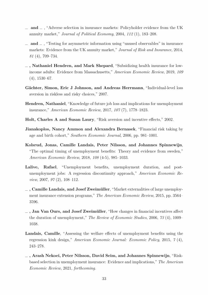
and , “Adverse selection in insurance markets: Policyholder evidence from the UKannuity market,” Journal of Political Economy, 2004, 112 (1), 183–208.

and , “Testing for asymmetric information using “unused observables” in insurancemarkets: Evidence from the UK annuity market,” Journal of Risk and Insurance, 2014,81 (4), 709–734.

, Nathaniel Hendren, and Mark Shepard, “Subsidizing health insurance for low-income adults: Evidence from Massachusetts,” American Economic Review, 2019, 109(4), 1530–67.

Gächter, Simon, Eric J Johnson, and Andreas Herrmann, “Individual-level lossaversion in riskless and risky choices,” 2007.

Hendren, Nathaniel, “Knowledge of future job loss and implications for unemploymentinsurance,” American Economic Review, 2017, 107 (7), 1778–1823.

Holt, Charles A and Susan Laury, “Risk aversion and incentive effects,” 2002.

Jianakoplos, Nancy Ammon and Alexandra Bernasek, “Financial risk taking byage and birth cohort,” Southern Economic Journal, 2006, pp. 981–1001.

Kolsrud, Jonas, Camille Landais, Peter Nilsson, and Johannes Spinnewijn,“The optimal timing of unemployment benefits: Theory and evidence from sweden,”American Economic Review, 2018, 108 (4-5), 985–1033.

Lalive, Rafael, “Unemployment benefits, unemployment duration, and post-unemployment jobs: A regression discontinuity approach,” American Economic Re-view, 2007, 97 (2), 108–112.

, Camille Landais, and Josef Zweimüller, “Market externalities of large unemploy-ment insurance extension programs,” The American Economic Review, 2015, pp. 3564–3596.

, Jan Van Ours, and Josef Zweimüller, “How changes in financial incentives affectthe duration of unemployment,” The Review of Economic Studies, 2006, 73 (4), 1009–1038.

Landais, Camille, “Assessing the welfare effects of unemployment benefits using theregression kink design,” American Economic Journal: Economic Policy, 2015, 7 (4),243–278.

, Arash Nekoei, Peter Nilsson, David Seim, and Johannes Spinnewijn, “Risk-based selection in unemployment insurance: Evidence and implications,” The AmericanEconomic Review, 2021, forthcoming.

33

Lindner, Attila and Balázs Reizer, “Frontloading the unemployment benefit: Anempirical assessment,” Technical Report, IEHAS Discussion Papers 2016.

McCrary, Justin, “Manipulation of the running variable in the regression discontinuitydesign: A density test,” Journal of Econometrics, 2008, 142 (2), 698–714.

Meyer, Bruce D, “Unemployment insurance and unemployment spells,” 1988.

Mueller, Andreas I, Johannes Spinnewijn, and Giorgio Topa, “Job Seekers’ Per-ceptions and Employment Prospects: Heterogeneity, Duration Dependence and Bias,”Technical Report, National Bureau of Economic Research 2018.

Ours, Jan C Van and Milan Vodopivec, “How shortening the potential duration ofunemployment benefits affects the duration of unemployment: Evidence from a naturalexperiment,” Journal of Labor economics, 2006, 24 (2), 351–378.

Parsons, Donald O, Torben Tranæs, and Helene Bie Lilleør, “Voluntary publicunemployment insurance,” 2003.

Paserman, M Daniele, “Job search and hyperbolic discounting: Structural estimationand policy evaluation,” The Economic Journal, 2008, 118 (531), 1418–1452.

Rothschild, Michael and Joseph Stiglitz, “Equilibrium in competitive insurancemarkets: An essay on the economics of imperfect information,” Quarterly Journal ofEconomics, 1976, 90 (4), 630–49.

Schmieder, Johannes F and Till Von Wachter, “The effects of unemployment insur-ance benefits: New evidence and interpretation,” Annual Review of Economics, 2016,8, 547–581.

, Till von Wachter, and Stefan Bender, “The effect of unemployment benefitsand nonemployment durations on wages,” American Economic Review, 2016, 106 (3),739–77.

Unédic, “Les allocataires qui travaillent et le cumul allocation-salaire : étude descrip-tive,” 2016.

, “Enquête auprès des allocataires qui travaillent,” 2018.

34

Tables and Figures

Table 1: Individual characteristics of compliers, takersand eligibles

Compliers Takers Eligible Nontakers All eligibles Noneligible Nontakers (3) - (1) (3) - (2) (5) - (4)

DemographicsAge 39.496 30.317 35.169 33.862 37.089 -4.327*** 4.852*** 3.228***

(0.324) (0.057) (0.024)Percentage of female 0.851 0.570 0.690 0.658 0.455 -0.161*** 0.120*** -0.203***

(0.012) (0.002) (0.001)QualificationExecutive 0.004 0.016 0.004 0.008 0.071 -0.000 -0.012*** 0.063***

(0.002) (0.001) (0.001)Intermediate occupation 0.016 0.024 0.005 0.013 0.030 -0.010*** -0.019*** 0.017***

(0.002) (0.001) (0.001)Skilled employee 0.620 0.580 0.513 0.539 0.515 -0.107*** -0.067*** -0.023***

(0.015) (0.003) (0.002)Skilled blue collar worker 0.210 0.265 0.222 0.239 0.245 0.012 -0.043*** 0.006***

(0.013) (0.003) (0.001)Unskilled employee 0.139 0.094 0.224 0.173 0.101 0.084*** 0.130*** -0.073***

(0.013) (0.002) (0.001)Unskilled blue collar worker 0.011 0.021 0.032 0.028 0.038 0.021*** 0.011*** 0.010***

(0.005) (0.001) (0.001)Level of educationNo education 0.039 0.023 0.041 0.036 0.030 0.002 0.017*** -0.006***

(0.005) (0.001) (0.000)Elementary school completed 0.022 0.011 0.020 0.018 0.011 -0.002 0.009*** -0.007***

(0.004) (0.001) (0.000)6th to 8th grade 0.024 0.013 0.023 0.020 0.015 -0.001 0.010*** -0.005***

(0.004) (0.001) (0.000)Middle school completed 0.048 0.042 0.060 0.055 0.040 0.012* 0.019*** -0.016***

(0.006) (0.001) (0.000)10th to 11th grade 0.015 0.011 0.016 0.014 0.012 0.001 0.005*** -0.002***

(0.003) (0.001) (0.000)Vocational diploma 0.424 0.469 0.405 0.422 0.367 -0.019 -0.064*** -0.055***

(0.013) (0.002) (0.001)High school diploma - Baccalaureate 0.247 0.228 0.255 0.248 0.253 0.008 0.028*** 0.005***

(0.011) (0.002) (0.001)Two-year Higher education degree 0.101 0.111 0.094 0.099 0.140 -0.007 -0.018*** 0.042***

(0.008) (0.001) (0.001)Three to four-year Higher education degree 0.056 0.056 0.058 0.057 0.073 0.002 0.001 0.016***

(0.006) (0.001) (0.001)Five-year and more Higher education degree 0.025 0.036 0.029 0.031 0.059 0.004 -0.007*** 0.028***

(0.004) (0.001) (0.001)

Rights’ characteristicsTenure 395.287 393.067 681.725 632.185 917.700 286.438*** 288.658*** 285.515***

(66.979) (9.367) (5.436)Part-time coefficient 0.694 0.689 0.645 0.650 0.958 -0.049*** -0.044*** 0.308***

(0.013) (0.002) (0.000)Number of unemployment spells over the period 1.336 1.370 2.811 2.423 2.471 1.475*** 1.441*** 0.048***

(0.073) (0.012) (0.005)PBD of the former right 446.454 468.780 550.358 540.413 564.500 103.904*** 81.578*** 24.087***

(11.563) (1.725) (0.607)Remaining PBD from former right 341.257 355.737 324.740 333.061 330.519 -16.517** -30.997*** -2.541***

(5.921) (1.063) (0.515)Observations 1508 62397 169234 231631 1664287 170742 231631 1895918

* p<0.05, ** p<0.01, *** p<0.001. Standard errors in parentheses.NOTE: This table compares the characteristics of compliers, takers, eligible nontakers and all eligibles, restricting to thesample under 20e. Compliers are those meeting the 20e but not the 30% condition, as they would not be treated absent the20e criterion. They are older and more frequently female than all other categories. They are also overrepresented amongskilled employees. They are typically found in preschool assistant occupations, where income fluctuations are common, aswage depends on the number of children cared for. Eligibles show characteristics associated with a lower attachment to thelabor market compared with noneligible nontakers, whereas, among them, takers are younger, more skilled and educated.

35

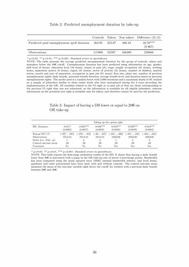
Table 2: Predicted unemployment duration by take-up

Controls Takers Non takers Difference (3)-(2)Predicted paid unemployment spell duration 263.95 253.67 286.43 32.76***

(0.967)

Observations 115900 62397 166269 228666

* p<0.05, ** p<0.01, *** p<0.001. Standard errors in parentheses.NOTE: The table presents the average predicted unemployment duration for the group of controls, takers andnontakers below the 20e cutoff. Unemployment duration has been predicted using information on age, gender,skill level (6 items), education level (10 items), tenure in past job, wage, sought occupation (81 items), workinghours, separation motive (8 items), region (31 items), sector of activity (21 items), number of children, maritalstatus, month and year of separation, occupation in past job (81 items), firm size, plant size, number of previousunemployment rights, daily benefit, potential benefit duration, average benefit level, and duration based on previousunemployment rights. The model used is a random forest with 2,000 iterations and a maximum depth of 50, trainedon a sample of jobseekers similar to those under study who were unemployed during the 2 years preceding theimplementation of the OR. All variables related to the UI right or to past job or firm are those corresponding tothe previous UI right that was not exhausted, as the information is available for all eligible jobseekers, whereasinformation on the potential new right is available only for takers, and therefore cannot be used for the prediction.

Table 3: Impact of having a DB lower or equal to 20e onOR take-up

Taking up the option rightRD_Estimate -0.011* -0.062*** -0.046*** -0.016*** -0.039*** -0.044***

(0.0063) (0.0057) (0.0058) (0.0058) (0.0049) (0.0063)Robust 95% CI [-.027 ; -.001] [-.076 ; -.052] [-.06 ; -.037] [-.031 ; -.006] [-.051 ; -.031] [-.058 ; -.031]Observations 1914144 1914144 1914144 1882340 1882340 1882340Order Loc. Poly. (p) 1 2 3 1 2 3Control outcome mean .09 .09 .09 .09 .09 .09Covariates No No No Yes Yes Yes

* p<0.05, ** p<0.01, *** p<0.001. Standard errors in parentheses.NOTE: This table reports the first-stage estimation results of the RD. It shows that having a daily benefitlower than 20e is associated with a jump in the OR take-up rate of about 4 percentage points. Bandwidthhas been computed using the mean squared error (MSE) optimal bandwidth selector, and local linear,quadratic and cubic polynomials have been used, with and without controls. The control outcome meanmeasures the mean of the outcome variable right above the cutoff, for workers with a previous daily benefitbetween 20e and 30e.

36

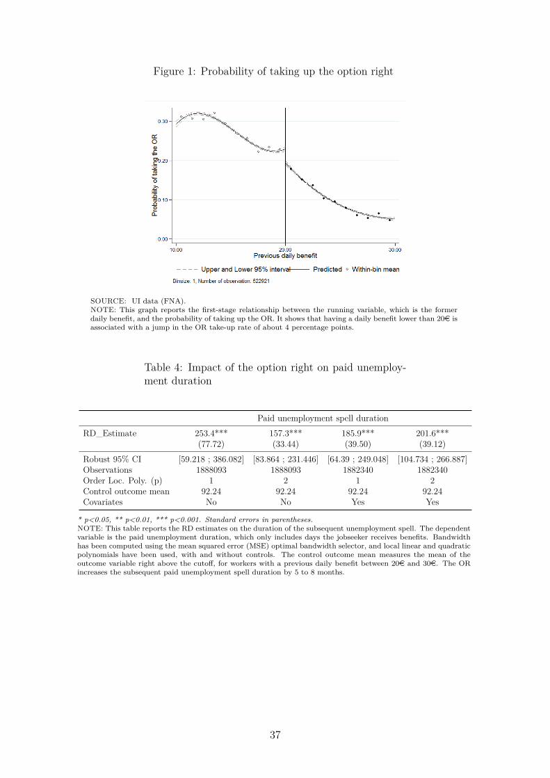
Figure 1: Probability of taking up the option right

SOURCE: UI data (FNA).NOTE: This graph reports the first-stage relationship between the running variable, which is the formerdaily benefit, and the probability of taking up the OR. It shows that having a daily benefit lower than 20e isassociated with a jump in the OR take-up rate of about 4 percentage points.

Table 4: Impact of the option right on paid unemploy-ment duration

Paid unemployment spell durationRD_Estimate 253.4*** 157.3*** 185.9*** 201.6***

(77.72) (33.44) (39.50) (39.12)Robust 95% CI [59.218 ; 386.082] [83.864 ; 231.446] [64.39 ; 249.048] [104.734 ; 266.887]Observations 1888093 1888093 1882340 1882340Order Loc. Poly. (p) 1 2 1 2Control outcome mean 92.24 92.24 92.24 92.24Covariates No No Yes Yes

* p<0.05, ** p<0.01, *** p<0.001. Standard errors in parentheses.NOTE: This table reports the RD estimates on the duration of the subsequent unemployment spell. The dependentvariable is the paid unemployment duration, which only includes days the jobseeker receives benefits. Bandwidthhas been computed using the mean squared error (MSE) optimal bandwidth selector, and local linear and quadraticpolynomials have been used, with and without controls. The control outcome mean measures the mean of theoutcome variable right above the cutoff, for workers with a previous daily benefit between 20e and 30e. The ORincreases the subsequent paid unemployment spell duration by 5 to 8 months.

37

Figure 2: Paid unemployment spell duration

SOURCE: UI data (FNA).NOTE: This graph reports the second-stage relationship between the running variable, which is theformer daily benefit, and the duration of the subsequent unemployment spell (second-order polynomial).The unemployment spell is defined as the paid unemployment spell, that is, the addition of the days thejobseeker receives benefits. It shows that having a daily benefit lower than 20e is associated with a jumpin the duration of the paid unemployment spell from about 97 to 104 days.

Figure 3: Full unemployment spell duration

SOURCE: UI data (FNA).NOTE: This graph reports the second-stage relationship between the running variable, which is theformer daily benefit, and the duration of the subsequent unemployment spell (second-order polynomial).The unemployment spell is defined as the full unemployment spell, that is, the addition of all the daysthe jobseeker is registered as unemployed, regardless whether receiving benefits or not. It shows thathaving a daily benefit lower than 20e is associated with a jump in the duration of the full unemploymentspell from about 148 to 161 days.

38

Table 5: Impact of the option right on full unemploy-ment duration

Full unemployment spell durationRD_Estimate 361.7*** 335.0*** 384.3*** 472.4***

(30.86) (49.38) (46.81) (63.20)Robust 95% CI [275.388 ; 408.345] [225.373 ; 423.782] [299.185 ; 493.74] [304.341 ; 586.861]Observations 1888093 1888093 1882340 1882340Order Loc. Poly. (p) 1 2 1 2Control outcome mean 145.84 145.84 145.84 145.84Covariates No No Yes Yes

* p<0.05, ** p<0.01, *** p<0.001. Standard errors in parentheses.NOTE: This table reports the RD estimates on the duration of the subsequent unemployment spell. The dependentvariable is the total unemployment duration, including days the jobseeker is registered as unemployed, regardlesswhether receiving benefits or not. Bandwidth has been computed using the mean squared error (MSE) optimalbandwidth selector, and local linear and quadratic polynomials have been used, with and without controls. Thecontrol outcome mean measures the mean of the outcome variable right above the cutoff, for workers with a previousdaily benefit between 20e and 30e. The OR increases the subsequent full unemployment spell duration by about12 months.

Table 6: Impact of the option right on the total numberof days on UI benefits

Total number of days receiving UI benefits after ORRD_Estimate 182.3 1.6 8.9 43.2

(182.28) (36.91) (31.22) (41.07)Robust 95% CI [-265.242 ; 486.825] [-84.771 ; 72.162] [-79.563 ; 67.175] [-58.647 ; 115.317]Observations 1888093 1888093 1882340 1882340Order Loc. Poly. (p) 1 2 1 2Control outcome mean 136.07 136.07 136.07 136.07Covariates No No Yes Yes

* p<0.05, ** p<0.01, *** p<0.001. Standard errors in parentheses.NOTE: This table reports the RD estimates on the total number of days on UI benefits over the whole observedperiod (October 2014–May 2017). Bandwidth has been computed using the mean squared error (MSE) optimalbandwidth selector, and local linear and quadratic polynomials have been used, with and without controls. Thecontrol outcome mean measures the mean of the outcome variable right above the cutoff, for workers with a previousdaily benefit between 20e and 30e. The OR does not have a significant impact on the total number of days on UIbenefits.

39

Table 7: Impact of the option right on the total numberof days registered as unemployed

Total number of days unemployed after ORRD_Estimate 180.7 134.8** 176.5*** 226.0***

(190.25) (52.73) (43.28) (53.01)Robust 95% CI [-255.745 ; 534.962] [20.595 ; 233.659] [58.228 ; 261.538] [124.935 ; 348.938]Observations 1888093 1888093 1882340 1882340Order Loc. Poly. (p) 1 2 1 2Control outcome mean 206.02 206.02 206.02 206.02Covariates No No Yes Yes

* p<0.05, ** p<0.01, *** p<0.001. Standard errors in parentheses.NOTE: This table reports the RD estimates on the total number of days registered as unemployed over the wholeobserved period (October 2014–May 2017). Bandwidth has been computed using the mean squared error (MSE)optimal bandwidth selector, and local linear and quadratic polynomials have been used, with and without controls.The control outcome mean measures the mean of the outcome variable right above the cutoff, for workers with aprevious daily benefit between 20e and 30e. The OR increases the total number of days registered as unemployedby about 180 days in the linear specification.

Table 8: Impact of OR on the probability to exhaustbenefits

Probability of exhausting UI benefitsRD_Estimate 0.166*** 0.134*** 0.151*** 0.153***

(0.0530) (0.0488) (0.0493) (0.0519)Robust 95% CI [.031 ; .275] [.016 ; .222] [.026 ; .253] [.029 ; .248]Observations 1914144 1914144 1882340 1882340Order Loc. Poly. (p) 1 2 1 2Control outcome mean .01 .01 .01 .01Covariates No No Yes Yes

* p<0.05, ** p<0.01, *** p<0.001. Standard errors in parentheses.NOTE: This table reports the RD estimates on the probability of exhausting UI benefits. Bandwidth has been com-puted using the mean squared error (MSE) optimal bandwidth selector, and local linear and quadratic polynomialshave been used, with and without controls. The control outcome mean measures the mean of the outcome variableright above the cutoff, for workers with a previous daily benefit between 20e and 30e. The right here refers to thenew right for those exercising the OR, and to the residual of the former right for those not exercising. If an eligiblenontaker has exhausted the residual and I do not observe that he recharges his right based on his last employmentspells, I assume that he is not able to recharge, and has exhausted all his entitlements. If a recharging is observedfor nontakers, I take into account the addition of the residual and the new right. The OR increases the probabilityof exhausting UI benefits by about 15 percentage points.

40

Figure 4: Impact on the probability of exhausting theUI right

SOURCE: UI data (FNA).NOTE: This graph reports the relationship between the probability of exhausting UI benefits and therunning variable, which is the level of the former daily benefit. The right here refers to the new right forthose exercising the OR, and to the residual from the former right for those not exercising. If an eligiblenontaker has exhausted the residual and I do not observe that he recharges his right based on his lastemployment spells, I assume that he is not able to recharge, and has exhausted all his entitlements. If arecharging is observed for nontakers, I take into account the addition of the remainder and the new right.The probability jumps at the threshold from 4.1% to 5.7%.

Table 9: Impact of the option right on the probabilityof working within the spell

Has worked during unemployment spellRD_Estimate 1.422*** 1.143*** 1.175*** 1.221***

(0.3437) (0.1740) (0.1626) (0.2022)Robust 95% CI [.642 ; 2.167] [.763 ; 1.498] [.905 ; 1.647] [.802 ; 1.692]Observations 1914144 1914144 1882340 1882340Order Loc. Poly. (p) 1 2 1 2Control outcome mean .39 .39 .39 .39Covariates No No Yes Yes

* p<0.05, ** p<0.01, *** p<0.001. Standard errors in parentheses.NOTE: This table reports the RD estimates on the probability of working within the subsequent unemploymentspell, while staying registered as unemployed. Bandwidth has been computed using the mean squared error (MSE)optimal bandwidth selector, and local linear and quadratic polynomials have been used, with and without controls.The control outcome mean measures the mean of the outcome variable right above the cutoff, for workers with aprevious daily benefit between 20e and 30e. The OR increases the probability of working during the spell by morethan 100 percentage points, because the RD estimation does not account for the binary nature of the dependentvariable.

41

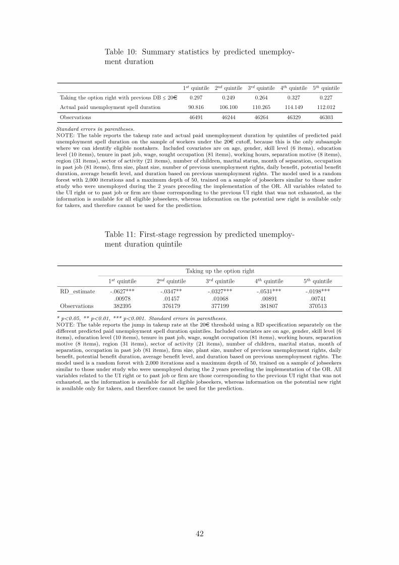
Table 10: Summary statistics by predicted unemploy-ment duration

1st quintile 2nd quintile 3rd quintile 4th quintile 5th quintileTaking the option right with previous DB ≤ 20e 0.297 0.249 0.264 0.327 0.227Actual paid unemployment spell duration 90.816 106.100 110.265 114.149 112.012

Observations 46491 46244 46264 46329 46303

Standard errors in parentheses.NOTE: The table reports the takeup rate and actual paid unemployment duration by quintiles of predicted paidunemployment spell duration on the sample of workers under the 20e cutoff, because this is the only subsamplewhere we can identify eligible nontakers. Included covariates are on age, gender, skill level (6 items), educationlevel (10 items), tenure in past job, wage, sought occupation (81 items), working hours, separation motive (8 items),region (31 items), sector of activity (21 items), number of children, marital status, month of separation, occupationin past job (81 items), firm size, plant size, number of previous unemployment rights, daily benefit, potential benefitduration, average benefit level, and duration based on previous unemployment rights. The model used is a randomforest with 2,000 iterations and a maximum depth of 50, trained on a sample of jobseekers similar to those understudy who were unemployed during the 2 years preceding the implementation of the OR. All variables related tothe UI right or to past job or firm are those corresponding to the previous UI right that was not exhausted, as theinformation is available for all eligible jobseekers, whereas information on the potential new right is available onlyfor takers, and therefore cannot be used for the prediction.

Table 11: First-stage regression by predicted unemploy-ment duration quintile

Taking up the option right1st quintile 2nd quintile 3rd quintile 4th quintile 5th quintile

RD_estimate -.0627*** -.0347** -.0327*** -.0531*** -.0198***.00978 .01457 .01068 .00891 .00741

Observations 382395 376179 377199 381807 370513

* p<0.05, ** p<0.01, *** p<0.001. Standard errors in parentheses.NOTE: The table reports the jump in takeup rate at the 20e threshold using a RD specification separately on thedifferent predicted paid unemployment spell duration quintiles. Included covariates are on age, gender, skill level (6items), education level (10 items), tenure in past job, wage, sought occupation (81 items), working hours, separationmotive (8 items), region (31 items), sector of activity (21 items), number of children, marital status, month ofseparation, occupation in past job (81 items), firm size, plant size, number of previous unemployment rights, dailybenefit, potential benefit duration, average benefit level, and duration based on previous unemployment rights. Themodel used is a random forest with 2,000 iterations and a maximum depth of 50, trained on a sample of jobseekerssimilar to those under study who were unemployed during the 2 years preceding the implementation of the OR. Allvariables related to the UI right or to past job or firm are those corresponding to the previous UI right that was notexhausted, as the information is available for all eligible jobseekers, whereas information on the potential new rightis available only for takers, and therefore cannot be used for the prediction.

42

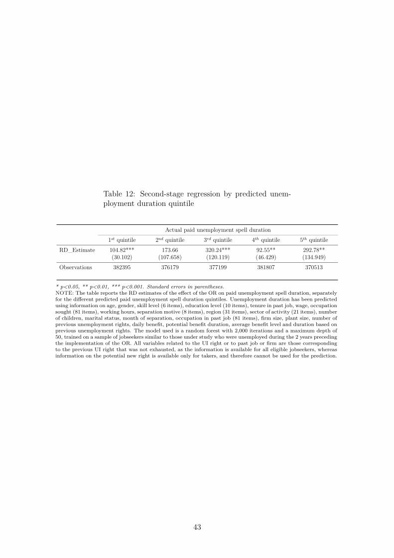
Table 12: Second-stage regression by predicted unem-ployment duration quintile

Actual paid unemployment spell duration1st quintile 2nd quintile 3rd quintile 4th quintile 5th quintile

RD_Estimate 104.82*** 173.66 320.24*** 92.55** 292.78**(30.102) (107.658) (120.119) (46.429) (134.949)

Observations 382395 376179 377199 381807 370513

* p<0.05, ** p<0.01, *** p<0.001. Standard errors in parentheses.NOTE: The table reports the RD estimates of the effect of the OR on paid unemployment spell duration, separatelyfor the different predicted paid unemployment spell duration quintiles. Unemployment duration has been predictedusing information on age, gender, skill level (6 items), education level (10 items), tenure in past job, wage, occupationsought (81 items), working hours, separation motive (8 items), region (31 items), sector of activity (21 items), numberof children, marital status, month of separation, occupation in past job (81 items), firm size, plant size, number ofprevious unemployment rights, daily benefit, potential benefit duration, average benefit level and duration based onprevious unemployment rights. The model used is a random forest with 2,000 iterations and a maximum depth of50, trained on a sample of jobseekers similar to those under study who were unemployed during the 2 years precedingthe implementation of the OR. All variables related to the UI right or to past job or firm are those correspondingto the previous UI right that was not exhausted, as the information is available for all eligible jobseekers, whereasinformation on the potential new right is available only for takers, and therefore cannot be used for the prediction.

43

Appendices

A Institutional background

Figure A1: Option right trade-off

NOTE: This diagram illustrates the different possibilities faced by a worker eligible for the OR. Right 1refers to the first right he has opened and not entirely consumed. At the end of the first employment spell,the individual has not worked enough to be eligible for the OR; he then automatically resumes right 1. Atthe end of the second employment spell, he has accumulated 6 months of employment. As the daily benefitassociated with right 1 is lower than 20e, he is entitled to exercise the OR. If he does so, he will benefit froma new 6-month right based on his last employment spells. If he does not exercise his OR, he will benefitfrom the residual of right 1 (duration = 14 – 4 – 2 = 8 months). At the end of right 1, he will be able toclaim right 2.

B Additional descriptive statistics

Table B1: Sample composition

20e condition 30% ratio condition TotalSimilar – – 2,209,471Eligible nontakers 210,116 ? 210,116Takers 71,525 128,441 139,254

NOTE: This tables details the composition of the sample I am working on, classified by eligibility criterion.Similar refers to workers similar to eligible workers, as they had opened a UI right in the past that they didnot entirely consume, but with a daily benefit higher than 20e. Eligible nontakers refer to eligible workerswho chose not to take the OR. I can only identify them under the 20e condition, as I have no informationon the new potential right for nontakers. Takers refer to those choosing the OR, that is, choosing the higherlevel of benefits. We count every unemployment spell meeting the eligibility condition, whereas for takers,we count one taker per right, as the OR can only be exercised at the beginning of the right (exercising it, bydefinition, leads to the opening of a new right; then, we cannot observe a person exercising the OR at thebeginning of a spell within a right). The addition of takers meeting the 20e condition with takers meetingthe 30% ratio condition is greater than the totality of takers as both conditions are not mutually exclusive.

44

Table B2: New and former right characteristics of takers

All takers Takers based on the 20e criterion CompliersAverage ratio between new and former DB 2.25 2.79 1.18Average ratio between new and former PBD 1.07 1.03 1.38Average ratio between new PBD and the remaining PBD 1.35 1.27 1.65Average ratio between total PBD if taking up or not taking up .593 .575 .646

NOTE: This table shows the characteristics associated with the former and the new rights for takers, decomposedby eligibility criterion. Compliers are those taking up the OR under the 20e condition, but not fulfilling the 30%criterion. By construction, the ratio of the new and the former daily benefits is lower for them, as it is constrainedto be under 1.3. However, they lose less in terms of duration, as shown by the last row.

C Assumptions of the RDD

Figure C1: McCrary test on previous DB distribution

SOURCE: UI data (FNA).NOTE: This graph shows the McCrary (2008) test (binsize = 1, bandwidth = 10) performed on the previousdaily benefit distribution to test the hypothesis of continuity of the running variable distribution at thethreshold. The density exhibits no discontinuity at the cutoff.

45

Figure C2: RD estimates on covariates

SOURCE: UI data (FNA).NOTE: This graphs tests the assumption of continuity in the distribution of covariates at the eligibilitythreshold by using each covariate as a dependent variable in the RDD regression. Bandwidth has beencomputed using the mean squared error (MSE) optimal bandwidth selector, and a local quadratic polynomialis used. The reported RD coefficients do no appear significant, except for the tenure variable.

Table C1: Impact on paid unemployment spell durationcontrolling for predicted unemployment duration

Paid unemployment spell durationRD_Estimate 253.4*** 157.3*** 185.9*** 201.6*** 114.6*** 151.6***

(77.72) (33.44) (39.50) (39.12) (30.11) (34.93)Robust 95% CI [59.218 ; 386.082] [83.864 ; 231.446] [64.39 ; 249.048] [104.734 ; 266.887] [28.926 ; 165.39] [75.036 ; 216.544]Observations 1888093 1888093 1882340 1882340 532111 532111Order Loc. Poly. (p) 1 2 1 2 1 2Control outcome mean 92.24 92.24 92.24 92.24 92.24 92.24Covariates No No Yes Yes Predicted unemployment duration Predicted unemployment duration

* p<0.05, ** p<0.01, *** p<0.001. Standard errors in parentheses.NOTE: This table reproduces the main result on the impact of the OR on the duration of the subsequent paidunemployment spell, without controls (columns 1-2), controlling for age, gender and education (columns 3-4), andcontrolling for predicted unemployment duration. The RD is estimated with the optimal bandwidth (MSE criterion),and local linear and quadratic polynomials are used. Unemployment duration is predicted using a sample of similarworkers unemployed during the two years preceding the introduction of the option right, and performing an out-of-sampleprediction on the sample under study. Included variables are age, gender, skill level (5 categories), education level(10 categories), sought occupation (14 categories), part-time coefficient, region of residence (31 categories), sector ofactivity (11 categories), month of contract termination, number of children, family situation (5 categories), previousoccupation (81 categories), firm and plant size. A flexible linear model is used, yielding a R2 equal to 7% and a RMSEequal to 281. The rather low R2 can be explained by the fact that I do not include any variable related to the UI entitlements.

D Additional tables and figures

46

Table D1: Impact of the option right on paid unemploy-ment duration – Reduced-Form estimates

Paid unemployment spell durationRD_Estimate -7.6*** -8.5*** -7.1*** -8.3***

(1.15) (1.52) (1.14) (1.51)Robust 95% CI [-9.609 ; -4.562] [-12.182 ; -5.715] [-9.252 ; -4.214] [-12.044 ; -5.656]Observations 1888093 1888093 1882340 1882340Order Loc. Poly. (p) 1 2 1 2Control outcome mean 92.24 92.24 92.24 92.24Covariates No No Yes Yes

* p<0.05, ** p<0.01, *** p<0.001. Standard errors in parentheses.NOTE: This table reports the reduced-form estimates from the RD regressions on the duration of the subsequentunemployment spell. The dependent variable is the paid unemployment duration, which only includes days thejobseeker receives benefits. Bandwidth has been computed using the mean squared error (MSE) optimal bandwidthselector, and local linear and quadratic polynomials have been used, with and without controls. The control outcomemean measures the mean of the outcome variable right above the cutoff, for workers with a previous daily benefitbetween 20e and 30e. Having a daily benefit above 20e decreases the subsequent paid unemployment spell durationby 7 to 8 days.

Table D2: Impact of the option right on full unemploy-ment duration – Reduced-Form estimates

Full unemployment spell durationRD_Estimate -16.0*** -11.8*** -11.2*** -12.1***

(1.56) (1.61) (1.45) (1.60)Robust 95% CI [-18.755 ; -11.975] [-14.934 ; -7.929] [-14.114 ; -7.55] [-15.992 ; -9.187]Observations 1888093 1888093 1882340 1882340Order Loc. Poly. (p) 1 2 1 2Control outcome mean 145.84 145.84 145.84 145.84Covariates No No Yes Yes

* p<0.05, ** p<0.01, *** p<0.001. Standard errors in parentheses.NOTE: This table reports the reduced-form estimates from the RD regressions on the duration of the subsequentunemployment spell. The dependent variable is the total unemployment duration, including days the jobseeker isregistered as unemployed, regardless whether receiving benefits or not. Bandwidth has been computed using themean squared error (MSE) optimal bandwidth selector, and local linear and quadratic polynomials are used, withand without controls. The control outcome mean measures the mean of the outcome variable right above the cutoff,for workers with a previous daily benefit between 20e and 30e. Having a daily benefit above 20e decreases thesubsequent full unemployment spell duration by 11 to 16 days.

47

Figure D1: Impact of paid unemployment spell durationwith different bandwidths

SOURCE: UI data (FNA).NOTE: This graph reproduces the main result regarding the impact of the OR on the duration of thesubsequent paid unemployment spell, using different bandwidths and a local quadratic polynomial. Optimalbandwidth has been multiplied respectively by 0.5, 1.5, 2, 2.5, and 3. The results are overall similar, butstandard errors become very large when choosing a bandwidth equivalent to half of the optimal one.

48

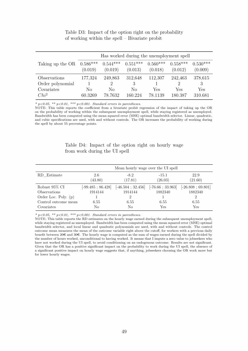
Table D3: Impact of the option right on the probabilityof working within the spell – Bivariate probit

Has worked during the unemployment spellTaking up the OR 0.586*** 0.544*** 0.551*** 0.560*** 0.558*** 0.530***

(0.019) (0.019) (0.013) (0.018) (0.012) (0.009)Observations 177,324 249,863 312,648 112,307 242,463 378,615Order polynomial 1 2 3 1 2 3Covariates No No No Yes Yes YesChi2 60.3269 78.7632 160.224 78.1139 180.387 310.681

* p<0.05, ** p<0.01, *** p<0.001. Standard errors in parentheses.NOTE: This table reports the coefficient from a bivariate probit regression of the impact of taking up the ORon the probability of working within the subsequent unemployment spell, while staying registered as unemployed.Bandwidth has been computed using the mean squared error (MSE) optimal bandwidth selector. Linear, quadratic,and cubic specifications are used, with and without controls. The OR increases the probability of working duringthe spell by about 55 percentage points.

Table D4: Impact of the option right on hourly wagefrom work during the UI spell

Mean hourly wage over the UI spellRD_Estimate 2.6 -8.2 -15.1 22.9

(43.80) (17.81) (26.03) (21.60)Robust 95% CI [-99.485 ; 86.428] [-46.504 ; 32.456] [-76.66 ; 33.963] [-26.808 ; 69.801]Observations 1914144 1914144 1882340 1882340Order Loc. Poly. (p) 1 2 1 2Control outcome mean 6.55 6.55 6.55 6.55Covariates No No Yes Yes

* p<0.05, ** p<0.01, *** p<0.001. Standard errors in parentheses.NOTE: This table reports the RD estimates on the hourly wage earned during the subsequent unemployment spell,while staying registered as unemployed. Bandwidth has been computed using the mean squared error (MSE) optimalbandwidth selector, and local linear and quadratic polynomials are used, with and without controls. The controloutcome mean measures the mean of the outcome variable right above the cutoff, for workers with a previous dailybenefit between 20e and 30e. The hourly wage is computed as the sum of wages earned during the spell divided bythe number of hours worked, unconditional to having worked. It means that I impute a zero value to jobseekers whohave not worked during the UI spell, to avoid conditioning on an endogenous outcome. Results are not significant.Given that the OR has a positive significant impact on the probability to work during the UI spell, the absence ofa significant positive impact on hourly wage suggests that, if anything, jobseekers choosing the OR work more butfor lower hourly wages.

49

Table D5: RDD coefficients on subpopulations

Taker Paid unemployment spell durationGenderMale -0.0610*** 206.4816***

(0.00825) (53.18824)Female -0.0196** 206.0439***

(0.00808) (42.15687)AgeLess than 25yo -0.0400*** 126.0005***

(0.01103) (25.34686)25 to 34yo -0.0323*** 119.4231**

(0.00752) (48.47335)35 to 44yo 0.0026 1227.3205

(0.00766) (2040.95902)45 to 54yo -0.0015 955.9014

(0.00776) (8831.66319)55yo and over -0.0085 983.7691

(0.01163) (1022.45154)Level of EducationLess than High school completed -0.0126 784.2686

(0.00895) (748.27010)Vocational High school degree -0.0002 348.6353*

(0.00933) (190.16862)General High school degree -0.0457*** 142.4035***

(0.01171) (37.81848)Higher Education -0.0338** 100.1442***

(0.01313) (32.73102)Skill levelExecutives and Intermediate occupations -0.0687* -275.1663

(0.03715) (336.64902)Skilled employees -0.0734*** 106.7712***

(0.01172) (36.77632)Skilled blue-collar workers 0.0061 87.9350

(0.02458) (117.07776)Unskilled employees and blue-collar workers -0.0257** 304.6875**

(0.01068) (147.96209)

* p<0.05, ** p<0.01, *** p<0.001. Standard errors in parentheses.NOTE: This table reports RD estimates by sub-groups. The first column displays the first-stage estimates of theprobability of taking up the OR on a binary variable indicating whether the former daily benefit was lower than 20e.The second column reports the second-stage estimates of the paid unemployment spell duration. The regressionshave been run separately on different gender, age, education, and skills groups. Bandwidth has been computedusing the mean squared error (MSE) optimal bandwidth selector and local linear polynomial has been used. Thesame regressions have been run using a local quadratic polynomial and results, available upon request, are similar.This table indicates for which subgroups the OR is particularly detrimental.

50

Table D6: Reduced-form estimates on paid UI spell du-ration using alternative definitions of the spell

Paid unemployment spell durationBefore any interruption 15-day definition 31-day definition 61-day definition 122-day definition

RD_Estimate -3.0*** -2.8** -3.1*** -2.7** -3.0*** -2.8** -3.4*** -3.3*** -3.7*** -3.5***(1.07) (1.25) (1.07) (1.26) (1.09) (1.26) (1.08) (1.27) (1.10) (1.30)

Robust 95% CI [-5.26 ; -.287] [-5.38 ; .135] [-5.391 ; -.395] [-5.373 ; .197] [-5.325 ; -.243] [-5.558 ; .028] [-5.588 ; -.632] [-6.037 ; -.427] [-5.912 ; -.887] [-6.305 ; -.567]Relative effect -5.3% -4.8% -5.2% -4.6% -5.1% -4.8% -5.6% -5.5% -6% -5.7%Observations 1131038 1131038 1131038 1131038 1131038 1131038 1131038 1131038 1131038 1131038Order Loc. Poly. (p) 1 2 1 2 1 2 1 2 1 2Control outcome mean 57.46 57.46 58.97 58.97 59.11 59.11 59.85 59.85 62.12 62.12Covariates No No No No No No No No No No

* p<0.05, ** p<0.01, *** p<0.001. Standard errors in parentheses.NOTE: This table reproduces the reduced-form RD estimates from the main regression on the paid unemploymentduration by taking alternative definitions of the unemployment spell. The preferred definition used throughoutthe paper is the gathering of days registered as unemployed without any interruption of at least 4 months. The4-month criterion has been chosen to ensure that the interruption reflects a stable return to work, and because it isthe minimum working requirement to be able to open a new UI right. The definition chosen should not affect theresult to the extent that we are comparing people in the direct neighborhood of the 20e cutoff, and that there is,a priori, no reason for the 4-month interruptions to be more or less frequent for a person earning 19e or 21e daily,apart from the effect of the OR. Nonetheless, it could be argued that if people exercising the OR are more prone toexperience very short employment spells while still being registered as unemployed, it could inflate the duration ofthe unemployment spell as defined earlier, even though these small employment periods do not enter the countingof the unemployment spell duration. To alleviate this concern, I perform the same analysis on the duration of thespell before interruption in payment (that is, going from subsidized unemployment to nonsubsidized unemploymentis considered an interruption here) of different durations. Note that the sample size is slightly lower because theraw data necessary to redefine the unemployment spell and available to the author do not include the whole originalsample. However, this subsample does not differ from the original one. Bandwidth has been computed using themean squared error (MSE) optimal bandwidth selector, and local linear and quadratic polynomials are used, withand without controls. The control outcome mean measures the mean of the outcome variable right above the cutoff,for workers with a previous daily benefit between 20e and 30e.Reduced-form estimates have been preferred to be able to compare their magnitude across definitions of the spellwithout being influenced by the size of the jump in takeup. Estimates are smaller in absolute terms but very similarrelative to the average duration of the different spells. Then, the measured impact on unemployment spell durationdoes not depend on the definition of the spell I choose to adopt.

51

Appendices - For online publication only

E Data appendix

Figure E1: Number of people exercising the option rightover time

SOURCE: UI data (FNA).NOTE: This graph displays the distribution of the number of people taking up the OR over time since itsimplementation in April 2015. We see an overall increase over time, with a seasonal pattern.

Table E1: Eligibility criteria distribution for takers

Takers based on the 20e criterion0 1

Takers based on the 30% ratio criterion 0 9,022 1,7911 58,707 69,734

NOTE: This table reports the distribution of takers according to both eligibility criteria.Note that most of the takers under the 20e condition also fulfill the 30% criterion, as it isuncommon to earn these very low levels of benefits for several consecutive unemploymentspells.

52

Figure E2: Starting date distribution

SOURCE: UI data (FNA).NOTE: This graph plots the distribution of workers with a daily benefit below and above the 20e threshold(within a window ranging between 16e and 24e), according to the starting date of the unemployment spell.It shows that control and treated workers are distributed in the same way across time, meaning that rightcensoring should not bias the results.

Figure E3: Probability of having a benefit lower than20e over time

SOURCE: UI data (FNA).NOTE: This graph plots the share of workers with a daily benefit equal to or lower than 20e over time.It shows the probability fo being eligible as part of the 20e criteria is rather stable over the period understudy.

F Additional descriptive statistics

53

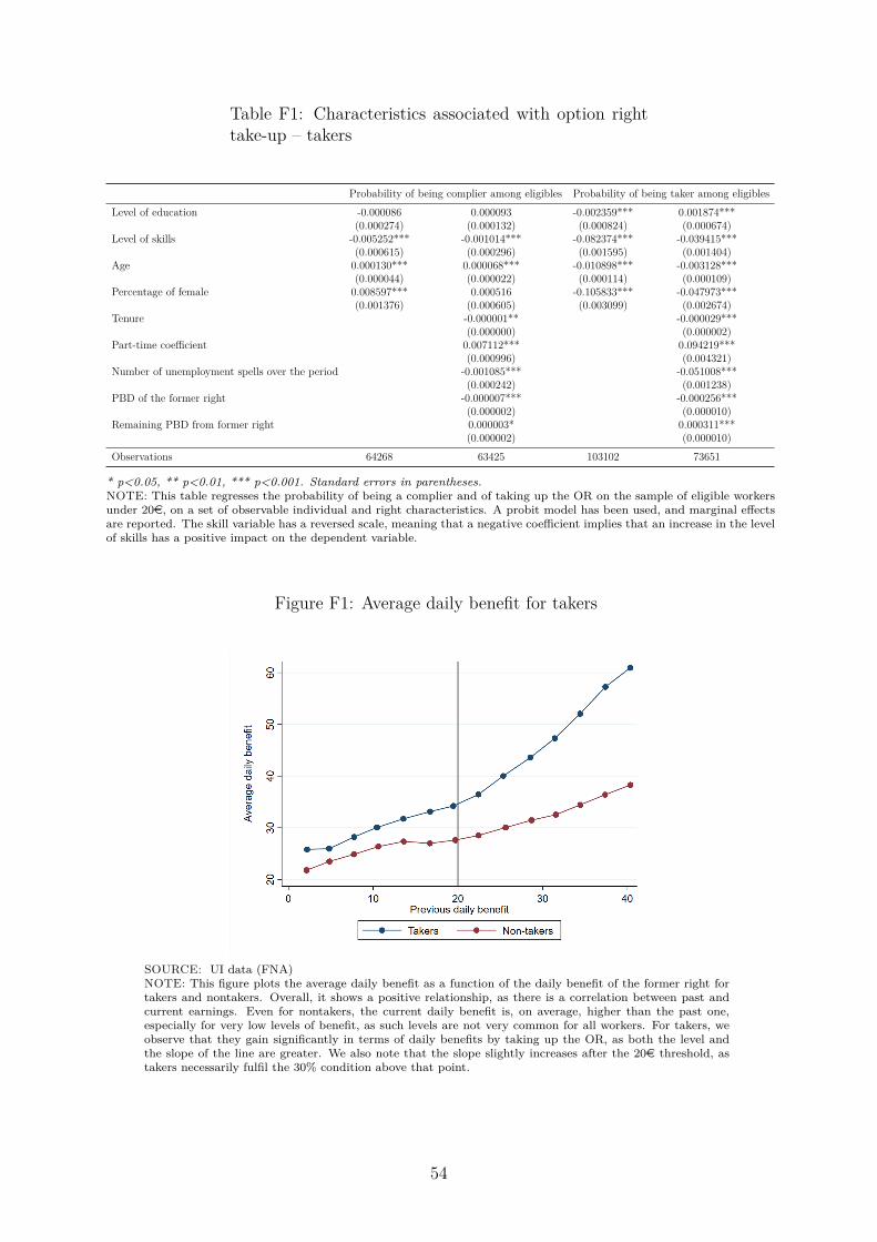
Table F1: Characteristics associated with option righttake-up – takers

Probability of being complier among eligibles Probability of being taker among eligiblesLevel of education -0.000086 0.000093 -0.002359*** 0.001874***

(0.000274) (0.000132) (0.000824) (0.000674)Level of skills -0.005252*** -0.001014*** -0.082374*** -0.039415***

(0.000615) (0.000296) (0.001595) (0.001404)Age 0.000130*** 0.000068*** -0.010898*** -0.003128***

(0.000044) (0.000022) (0.000114) (0.000109)Percentage of female 0.008597*** 0.000516 -0.105833*** -0.047973***

(0.001376) (0.000605) (0.003099) (0.002674)Tenure -0.000001** -0.000029***

(0.000000) (0.000002)Part-time coefficient 0.007112*** 0.094219***

(0.000996) (0.004321)Number of unemployment spells over the period -0.001085*** -0.051008***

(0.000242) (0.001238)PBD of the former right -0.000007*** -0.000256***

(0.000002) (0.000010)Remaining PBD from former right 0.000003* 0.000311***

(0.000002) (0.000010)Observations 64268 63425 103102 73651

* p<0.05, ** p<0.01, *** p<0.001. Standard errors in parentheses.NOTE: This table regresses the probability of being a complier and of taking up the OR on the sample of eligible workersunder 20e, on a set of observable individual and right characteristics. A probit model has been used, and marginal effectsare reported. The skill variable has a reversed scale, meaning that a negative coefficient implies that an increase in the levelof skills has a positive impact on the dependent variable.

Figure F1: Average daily benefit for takers

SOURCE: UI data (FNA)NOTE: This figure plots the average daily benefit as a function of the daily benefit of the former right fortakers and nontakers. Overall, it shows a positive relationship, as there is a correlation between past andcurrent earnings. Even for nontakers, the current daily benefit is, on average, higher than the past one,especially for very low levels of benefit, as such levels are not very common for all workers. For takers, weobserve that they gain significantly in terms of daily benefits by taking up the OR, as both the level andthe slope of the line are greater. We also note that the slope slightly increases after the 20e threshold, astakers necessarily fulfil the 30% condition above that point.

54

Figure F2: Average PBD for takers if taking up or nottaking up

SOURCE: UI data (FNA)NOTE: This figure plots the average potential benefit duration as a function of the daily benefit of theformer right for takers. I compute the potential PBD they would have had if they had not taken up theOR. Both lines follow the same pattern. Although the average PBD duration is much higher in the “if nottaking” scenario, takers are still entitled to a long duration in absolute terms.

Figure F3: Average PBD without taking into accountrecharging

SOURCE: UI data (FNA)NOTE: This figure plots the average PBD as a function of the daily benefit of the former right for takers andnontakers. In this graph, the PBD of nontakers corresponds to the duration of the remainder of the formerright. The total PBD, which is the duration of the remainder plus the duration of the new potential right,cannot be computed for nontakers. We observe that the remainder of the former right is slightly decreasingwith the level of previous benefit. It could be driven by the fact that the unemployment duration is generallypositively correlated with the level of benefits. The higher the daily benefit, the more the jobseeker willconsume of his right, and the less he will have left for future unemployment spells.

55

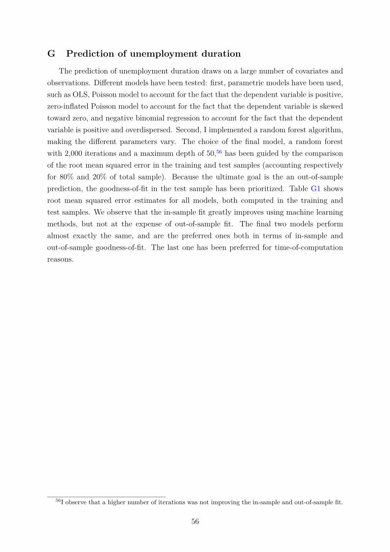
G Prediction of unemployment duration

The prediction of unemployment duration draws on a large number of covariates andobservations. Different models have been tested: first, parametric models have been used,such as OLS, Poisson model to account for the fact that the dependent variable is positive,zero-inflated Poisson model to account for the fact that the dependent variable is skewedtoward zero, and negative binomial regression to account for the fact that the dependentvariable is positive and overdispersed. Second, I implemented a random forest algorithm,making the different parameters vary. The choice of the final model, a random forestwith 2,000 iterations and a maximum depth of 50,56 has been guided by the comparisonof the root mean squared error in the training and test samples (accounting respectivelyfor 80% and 20% of total sample). Because the ultimate goal is the an out-of-sampleprediction, the goodness-of-fit in the test sample has been prioritized. Table G1 showsroot mean squared error estimates for all models, both computed in the training andtest samples. We observe that the in-sample fit greatly improves using machine learningmethods, but not at the expense of out-of-sample fit. The final two models performalmost exactly the same, and are the preferred ones both in terms of in-sample andout-of-sample goodness-of-fit. The last one has been preferred for time-of-computationreasons.

56I observe that a higher number of iterations was not improving the in-sample and out-of-sample fit.

56

Table G1: Root mean squared error of models for theprediction of unemployment duration

Training sample Test sampleOLS 228.707 266.642Poisson 226.906 229.289Zero-Inflated Poisson 226.931 229.295Negative Binomial 230.362 231.726Random Forest (Iter=10, Max Depth=50) 102.389 236.684Random Forest (Iter=200, Max Depth=50) 86.750 226.161Random Forest (Iter=2000, Max Depth=1000) 86.154 225.612Random Forest (Iter=2000, Max Depth=50) 86.193 225.668

* p<0.05, ** p<0.01, *** p<0.001. Standard errors in parentheses.NOTE: This table reports the root mean squared error computed in the training sample(80% of the sample) and in the test sample (20% of the sample) for each model. For allmodels, included covariates are age, gender, skill level (6 items), education level (10 items),tenure in past job, wage, sought occupation (81 items), working hours, separation motive (8items), region (31 items), sector of activity (21 items), number of children, marital status,month and year of separation, occupation in past job (81 items), firm size, plant size, numberof previous unemployment rights, daily benefit, potential benefit duration, average benefitlevel, and duration based on previous unemployment rights. The regression has been madeon jobseekers similar to those under study who were unemployed during the 2 years precedingthe implementation of the OR (April 2013–March 2015). All variables related to the UI rightor to past job or firm are those corresponding to the previous UI right that was not exhausted,as the information is available for all eligible jobseekers, whereas information on the potentialnew right is available only for takers, and therefore cannot be used for the prediction.

Figures G1 and G2 show the distribution of the actual and predicted unemploymentduration for each model. Among the parametric ones, the negative binomial predictionfits better low values and has a larger variance. This is even more the case when weexamine non-parametric models, in particular when the number of iterations increases.Both the visual inspection of the distributions and the RMSE point to random forestperforming better at predicting unemployment duration.

As a robustness check, I also report the prediction for takers and nontakers under20e using a flexible OLS (Table G2). If the level of unemployment duration is lowerin absolute terms than in my main model, the difference between takers and nontakersgoes in the same direction and is of the same order of magnitude (10% of the predictedduration of takers).

57

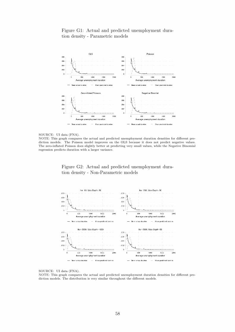
Figure G1: Actual and predicted unemployment dura-tion density - Parametric models

SOURCE: UI data (FNA).NOTE: This graph compares the actual and predicted unemployment duration densities for different pre-diction models. The Poisson model improves on the OLS because it does not predict negative values.The zero-inflated Poisson does slightly better at predicting very small values, while the Negative Binomialregression predicts duration with a larger variance.

Figure G2: Actual and predicted unemployment dura-tion density - Non-Parametric models

SOURCE: UI data (FNA).NOTE: This graph compares the actual and predicted unemployment duration densities for different pre-diction models. The distribution is very similar throughout the different models.

58

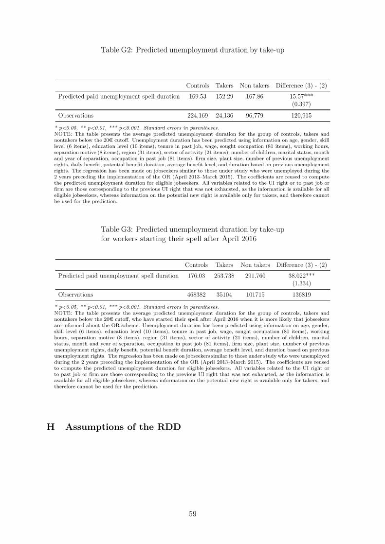
Table G2: Predicted unemployment duration by take-up

Controls Takers Non takers Difference (3) - (2)Predicted paid unemployment spell duration 169.53 152.29 167.86 15.57***

(0.397)

Observations 224,169 24,136 96,779 120,915

* p<0.05, ** p<0.01, *** p<0.001. Standard errors in parentheses.NOTE: The table presents the average predicted unemployment duration for the group of controls, takers andnontakers below the 20e cutoff. Unemployment duration has been predicted using information on age, gender, skilllevel (6 items), education level (10 items), tenure in past job, wage, sought occupation (81 items), working hours,separation motive (8 items), region (31 items), sector of activity (21 items), number of children, marital status, monthand year of separation, occupation in past job (81 items), firm size, plant size, number of previous unemploymentrights, daily benefit, potential benefit duration, average benefit level, and duration based on previous unemploymentrights. The regression has been made on jobseekers similar to those under study who were unemployed during the2 years preceding the implementation of the OR (April 2013–March 2015). The coefficients are reused to computethe predicted unemployment duration for eligible jobseekers. All variables related to the UI right or to past job orfirm are those corresponding to the previous UI right that was not exhausted, as the information is available for alleligible jobseekers, whereas information on the potential new right is available only for takers, and therefore cannotbe used for the prediction.

Table G3: Predicted unemployment duration by take-upfor workers starting their spell after April 2016

Controls Takers Non takers Difference (3) - (2)Predicted paid unemployment spell duration 176.03 253.738 291.760 38.022***

(1.334)

Observations 468382 35104 101715 136819

* p<0.05, ** p<0.01, *** p<0.001. Standard errors in parentheses.NOTE: The table presents the average predicted unemployment duration for the group of controls, takers andnontakers below the 20e cutoff, who have started their spell after April 2016 when it is more likely that jobseekersare informed about the OR scheme. Unemployment duration has been predicted using information on age, gender,skill level (6 items), education level (10 items), tenure in past job, wage, sought occupation (81 items), workinghours, separation motive (8 items), region (31 items), sector of activity (21 items), number of children, maritalstatus, month and year of separation, occupation in past job (81 items), firm size, plant size, number of previousunemployment rights, daily benefit, potential benefit duration, average benefit level, and duration based on previousunemployment rights. The regression has been made on jobseekers similar to those under study who were unemployedduring the 2 years preceding the implementation of the OR (April 2013–March 2015). The coefficients are reusedto compute the predicted unemployment duration for eligible jobseekers. All variables related to the UI right orto past job or firm are those corresponding to the previous UI right that was not exhausted, as the information isavailable for all eligible jobseekers, whereas information on the potential new right is available only for takers, andtherefore cannot be used for the prediction.

H Assumptions of the RDD

59

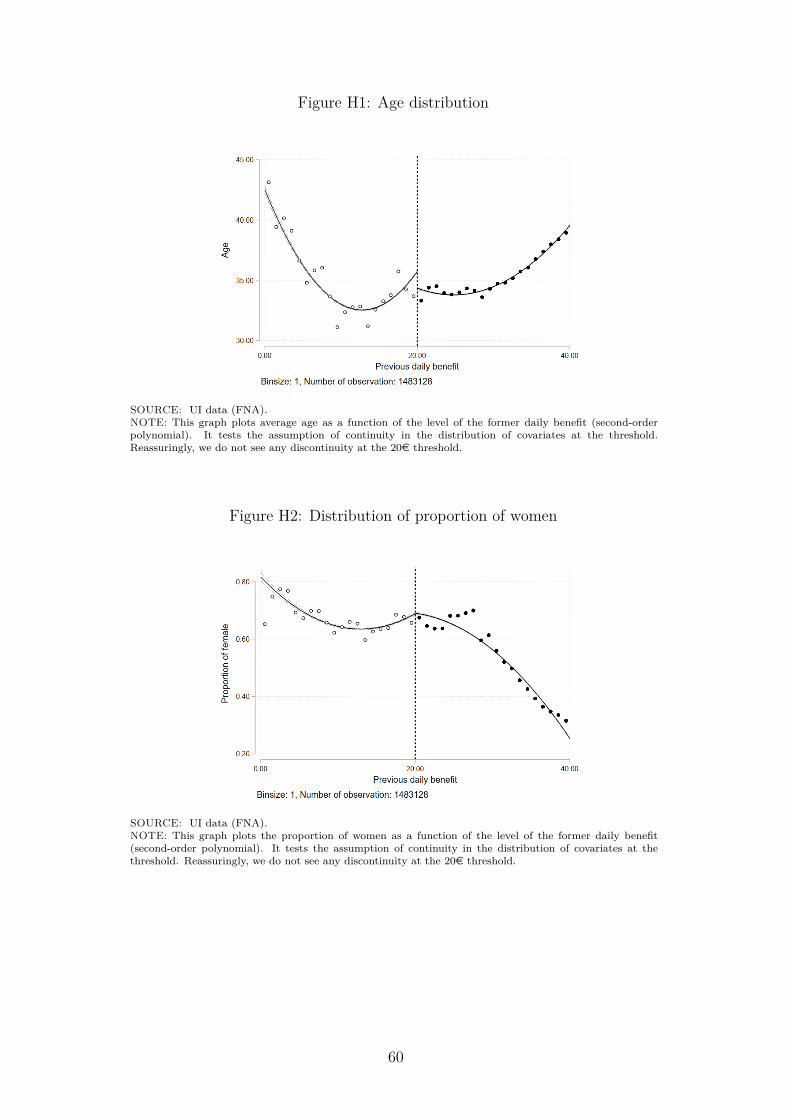
Figure H1: Age distribution

SOURCE: UI data (FNA).NOTE: This graph plots average age as a function of the level of the former daily benefit (second-orderpolynomial). It tests the assumption of continuity in the distribution of covariates at the threshold.Reassuringly, we do not see any discontinuity at the 20e threshold.

Figure H2: Distribution of proportion of women

SOURCE: UI data (FNA).NOTE: This graph plots the proportion of women as a function of the level of the former daily benefit(second-order polynomial). It tests the assumption of continuity in the distribution of covariates at thethreshold. Reassuringly, we do not see any discontinuity at the 20e threshold.

60

Figure H3: Level of education distribution

SOURCE: UI data (FNA).NOTE: This graph plots the average level of education as a function of the level of the former daily benefit(second-order polynomial). It tests the assumption of continuity in the distribution of covariates at thethreshold. Reassuringly, we do not see any discontinuity at the 20e threshold.

Figure H4: Skill distribution

SOURCE: UI data (FNA).NOTE: This graph plots average skill level as a function of the level of the former daily benefit (second-order polynomial). It tests the assumption of continuity in the distribution of covariates at the threshold.Reassuringly, we do not see any discontinuity at the 20e threshold.

61

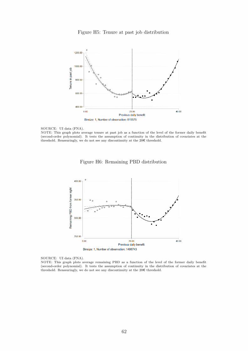
Figure H5: Tenure at past job distribution

SOURCE: UI data (FNA).NOTE: This graph plots average tenure at past job as a function of the level of the former daily benefit(second-order polynomial). It tests the assumption of continuity in the distribution of covariates at thethreshold. Reassuringly, we do not see any discontinuity at the 20e threshold.

Figure H6: Remaining PBD distribution

SOURCE: UI data (FNA).NOTE: This graph plots average remaining PBD as a function of the level of the former daily benefit(second-order polynomial). It tests the assumption of continuity in the distribution of covariates at thethreshold. Reassuringly, we do not see any discontinuity at the 20e threshold.

62

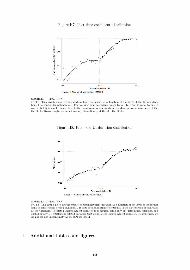
Figure H7: Part-time coefficient distribution

SOURCE: UI data (FNA).NOTE: This graph plots average working-hour coefficient as a function of the level of the former dailybenefit (second-order polynomial). The working-hour coefficient ranges from 0 to 1 and is equal to one incase of full-time employment. It tests the assumption of continuity in the distribution of covariates at thethreshold. Reassuringly, we do not see any discontinuity at the 20e threshold.

Figure H8: Predicted UI duration distribution

SOURCE: UI data (FNA).NOTE: This graph plots average predicted unemployment duration as a function of the level of the formerdaily benefit (second-order polynomial). It tests the assumption of continuity in the distribution of covariatesat the threshold. Predicted unemployment duration is computed using only pre-determined variables, andexcluding any UI entitlement-related variables that could affect unemployment duration. Reassuringly, wedo not see any discontinuity at the 20e threshold.

I Additional tables and figures

63

Table I1: Impact of paid unemployment spell durationwith different bandwidths

Paid unemployment spell durationLocal linear polynomial Local quadratic polynomial

RD_Estimate 208.5*** -939.3 178.1*** 163.3*** 155.3*** 759.9 145.1*** 202.9***(31.71) (1140.96) (35.98) (27.88) (34.90) (1546.81) (31.14) (39.13)

Robust 95% CI [111.838 ; 260.196] [-1665.932 ; 4907.587] [44.776 ; 262.732] [94.806 ; 262.23] [75.238 ; 216.045] [608.051 ; 8725.98] [81.841 ; 243.847] [-39.16 ; 162.104]Observations 1888093 1888093 1888093 1888093 1888093 1888093 1888093 1888093Order Loc. Poly. (p) 1 1 1 1 2 2 2 2Control outcome mean 92.24 92.24 92.24 92.24 92.24 92.24 92.24 92.24Bandwidth Optimal bandwith (OB) OB × .5 OB × 1.5 OB × 2 Optimal bandwith (OB) OB × .5 OB × 1.5 OB × 2

* p<0.05, ** p<0.01, *** p<0.001. Standard errors in parentheses.NOTE: This table reproduces the main result on the impact of the OR on the duration of the subsequent paid unem-ployment spell, using different bandwidths. The RD is estimated with the optimal bandwidth (MSE criterion), and theoptimal bandwidth (OB) multiplied by 0.5, 1.5 and 2. Local linear and quadratic polynomials are used. The results areoverall similar, but not significant when choosing a bandwidth equivalent to half of the optimal one.

64

Figure I1: Total number of days unemployed after theexercise of the option right

SOURCE: UI data (FNA).NOTE: This graph reports the second-stage relationship between the running variable, which is theformer daily benefit, and the total number of days registered as unemployed over the whole observedperiod (second-order polynomial). The observation period is between October 2014 and May 2017. Itshows that having a daily benefit lower than 20e is associated with a jump in the total number of daysregistered as unemployed from about 210 to 220 days.

Figure I2: Total number of days on UI benefits afterthe exercise of the option right

SOURCE: UI data (FNA).NOTE: This graph reports the second-stage relationship between the running variable, which is theformer daily benefit, and the total number of days on UI benefits over the whole observed period (second-order polynomial). The observation period is between October 2014 and May 2017. It shows that havinga daily benefit lower than 20e is associated with a jump in the total number of days on UI benefits fromabout 143 to 146 days.

65

Table I2: Probability of exhausting the UI right

% reaching the end ofthe right at the end of

the first U spell

% reaching the end ofthe right when takinginto account all U

spellsAll takers 12% 13.7%Takers with previous benefit ≤ 20e 15.2% 17.2%

NOTE: The first column shows the probability of exhausting the right at the end of the first unemployment spell,and the second takes into account all the unemployment spells.

Table I3: Impact of the option right on labor incomeearned over the spell

Labour income earned over the UI spellRD_Estimate 8918.2*** 7713.2*** 10771.2*** 9229.8***

(2100.18) (2301.79) (2843.83) (2476.81)Robust 95% CI [4885.951 ; 14272.303] [2724.9 ; 12667.919] [5592.068 ; 17788.017] [4825.408 ; 15335.848]Observations 766113 766113 766065 766065Order Loc. Poly. (p) 1 2 1 2Control outcome mean 1465.84 1465.84 1465.84 1465.84Covariates No No Yes Yes

* p<0.05, ** p<0.01, *** p<0.001. Standard errors in parentheses.NOTE: This table reports the RD estimates on the labor income earned during the subsequent unemployment spell,while remaining registered as unemployed. Bandwidth has been computed using the mean squared error (MSE)optimal bandwidth selector, and local linear and quadratic polynomials are used, with and without controls. Thecontrol outcome mean measures the mean of the outcome variable right above the cutoff, for workers with a previousdaily benefit between 20e and 30e. The OR increases the labor income earned during the spell by about 8,000e,depending on the specification. This result has been computed on the labor income conditional on having workedduring the spell, which is itself endogenous to the OR. Therefore, we cannot exclude that there is a compositioneffect mixing with the pure effect on labor income.

66

Table I4: Impact of the option right on the number ofhours worked during a spell

Number of hours worked over the UI spellRD_Estimate 700.2*** 838.5*** 746.3*** 1013.0***

(150.16) (257.00) (225.43) (346.77)Robust 95% CI [417.482 ; 1105.52] [232.625 ; 1326.769] [397.005 ; 1340.172] [247.225 ; 1768.913]Observations 766113 766113 766065 766065Order Loc. Poly. (p) 1 2 1 2Control outcome mean 131.46 131.46 131.46 131.46Covariates No No Yes Yes

* p<0.05, ** p<0.01, *** p<0.001. Standard errors in parentheses.NOTE: This table reports the RD estimates on the number of hours worked during the subsequent unemploymentspell, while staying registered as unemployed. Bandwidth has been computed using the mean squared error (MSE)optimal bandwidth selector, and local linear and quadratic polynomials are used, with and without controls. Thecontrol outcome mean measures the mean of the outcome variable right above the cutoff, for workers with a previousdaily benefit between 20e and 30e. The OR increases the number of hours worked during the spell by about 800hours, depending on the specification. This result has been computed on the number of hours conditional onhaving worked during the spell, which is itself endogenous to the OR. Therefore, we cannot exclude that there is acomposition effect mixing with the pure effect on the number of hours worked.

Table I5: Impact of the option right on the daily earn-ings over the subsequent spell

Daily earningsRD_Estimate 211.1*** 214.1*** 307.3*** 177.8***

(67.28) (61.98) (98.38) (66.53)Robust 95% CI [75.799 ; 371.121] [94.175 ; 360.654] [111.295 ; 527.484] [38.649 ; 314.652]Observations 1859860 1859860 1854187 1854187Order Loc. Poly. (p) 1 2 1 2Control outcome mean 31.12 31.12 31.12 31.12Covariates No No Yes Yes

* p<0.05, ** p<0.01, *** p<0.001. Standard errors in parentheses.NOTE: This table reports the RD estimates on the average level of daily earnings over the subsequent unemploymentspell. Bandwidth has been computed using the mean squared error (MSE) optimal bandwidth selector, and locallinear and quadratic polynomials are used, with and without controls. The control outcome mean measures themean of the outcome variable right above the cutoff, for workers with a previous daily benefit between 20e and 30e.Daily earnings are computed by dividing the sum of UI benefits and earnings from work by the duration of the UIspell. Earnings from work are measured only if the person stays registered as unemployed, which is likely for thetype of short unemployment spells that are not long enough to define the end of the UI spell. The duration of theUI spell is measured as the time elapsed between the starting and the ending dates of the spell, including potentialdays of interruptions.

67

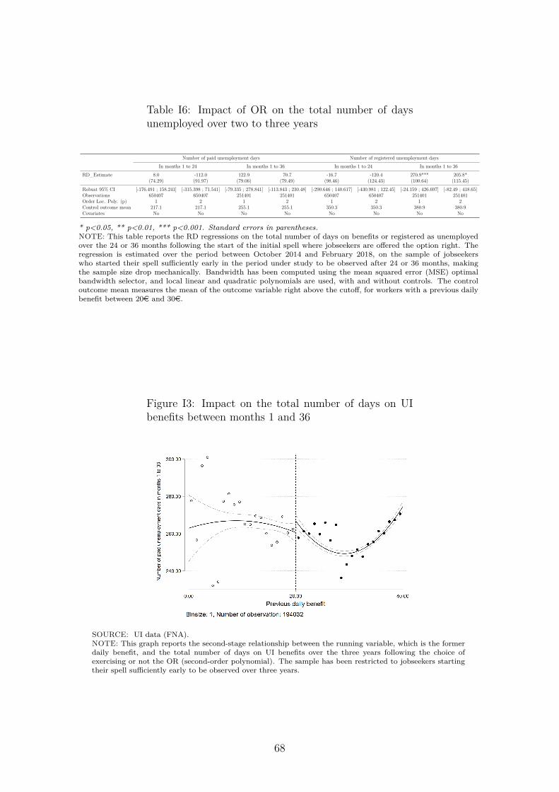
Table I6: Impact of OR on the total number of daysunemployed over two to three years

Number of paid unemployment days Number of registered unemployment daysIn months 1 to 24 In months 1 to 36 In months 1 to 24 In months 1 to 36

RD_Estimate 8.0 -112.0 122.9 70.7 -16.7 -120.4 270.9*** 205.8*(74.29) (91.97) (79.06) (79.49) (98.46) (124.43) (100.64) (115.45)

Robust 95% CI [-176.491 ; 158.241] [-315.398 ; 71.541] [-79.335 ; 278.841] [-113.843 ; 230.48] [-290.646 ; 140.617] [-430.981 ; 122.45] [-24.159 ; 426.697] [-82.49 ; 418.65]Observations 650407 650407 251401 251401 650407 650407 251401 251401Order Loc. Poly. (p) 1 2 1 2 1 2 1 2Control outcome mean 217.1 217.1 255.1 255.1 350.3 350.3 380.9 380.9Covariates No No No No No No No No

* p<0.05, ** p<0.01, *** p<0.001. Standard errors in parentheses.NOTE: This table reports the RD regressions on the total number of days on benefits or registered as unemployedover the 24 or 36 months following the start of the initial spell where jobseekers are offered the option right. Theregression is estimated over the period between October 2014 and February 2018, on the sample of jobseekerswho started their spell sufficiently early in the period under study to be observed after 24 or 36 months, makingthe sample size drop mechanically. Bandwidth has been computed using the mean squared error (MSE) optimalbandwidth selector, and local linear and quadratic polynomials are used, with and without controls. The controloutcome mean measures the mean of the outcome variable right above the cutoff, for workers with a previous dailybenefit between 20e and 30e.

Figure I3: Impact on the total number of days on UIbenefits between months 1 and 36

SOURCE: UI data (FNA).NOTE: This graph reports the second-stage relationship between the running variable, which is the formerdaily benefit, and the total number of days on UI benefits over the three years following the choice ofexercising or not the OR (second-order polynomial). The sample has been restricted to jobseekers startingtheir spell sufficiently early to be observed over three years.

68

Figure I4: Impact on the total number of days registeredas unemployed between months 1 and 36

SOURCE: UI data (FNA).NOTE: This graph reports the second-stage relationship between the running variable, which is the formerdaily benefit, and the total number of days registered as unemployed over the three years following thechoice of exercising or not the OR (second-order polynomial). The sample has been restricted to jobseekersstarting their spell sufficiently early to be observed over three years.

69

Table I7: Impact on the probability of being in paidunemployment

Probability of being in paid unemploymentIn month 3 In month 6 In month 12 In month 24

Taker=1 0.182*** 0.106* 0.123*** 0.140*** 0.068 0.070* 0.024 -0.029 -0.015 -0.006 0.161 -0.000(0.0514) (0.0561) (0.0362) (0.0415) (0.0596) (0.0395) (0.0564) (0.0546) (0.0518) (0.0184) (0.5355) (0.0106)

Observations 213773 209485 299629 277736 217824 300174 180755 181714 195848 11481 14412 19459Order Loc. Poly. (p) 1 2 3 1 2 3 1 2 3 1 2 3Control outcome mean .549 .549 .549 .384 .384 .384 .228 .228 .228 .002 .002 .002Covariates No No No No No No No No No No No No

* p<0.05, ** p<0.01, *** p<0.001. Standard errors in parentheses.NOTE: This table reports the impact of the OR on the probability of being in paid unemployment at different timesfollowing the decision whether to exercise the OR, using a bivariate probit regression. Bandwidth has been computedusing the mean squared error (MSE) optimal bandwidth selector, and linear, quadratic and cubic specifications areused. The control outcome mean measures the mean of the outcome variable right above the cutoff, for workerswith a previous daily benefit between 20e and 30e. It shows that the main effect occurs in the short term.

Table I8: Impact on the probability of being registeredas unemployed

Probability of being registered as unemployedIn month 3 In month 6 In month 12 In month 24

Taker=1 0.173*** 0.129*** 0.184*** 0.162*** 0.082 0.167*** 0.025 -0.115** -0.103** -0.010 0.002 -0.004(0.0346) (0.0317) (0.0176) (0.0558) (0.0507) (0.0384) (0.0688) (0.0559) (0.0523) (0.0207) (0.0363) (0.0090)

Observations 205119 227010 330930 191054 216171 261641 174038 172639 189891 11302 14303 19342Order Loc. Poly. (p) 1 2 3 1 2 3 1 2 3 1 2 3Control outcome mean .783 .783 .783 .627 .627 .627 .429 .429 .429 .004 .004 .004Covariates No No No No No No No No No No No No

* p<0.05, ** p<0.01, *** p<0.001. Standard errors in parentheses.NOTE: This table reports the impact of the OR on the probability of being registered as unemployed at differenttimes following the decision whether to exercise the OR, using a bivariate probit regression. Bandwidth has beencomputed using the mean squared error (MSE) optimal bandwidth selector, and linear, quadratic and cubic specifi-cations are used. The control outcome mean measures the mean of the outcome variable right above the cutoff, forworkers with a previous daily benefit between 20e and 30e. It shows that the main effect occurs in the short term.

70

Figure I5: Permutation test for the impact on the dura-tion of the paid unemployment spell

SOURCE: UI data (FNA).NOTE: This permutation test randomly selects a cutoff value between 0 and 100 and computes the corre-sponding RD reduced-form estimate (1,000 replications). The two dashed lines indicates values 0.05 and0.95 of the CDF. We observe that the true effect is outside this confidence interval, confirming that it theOR has a significant effect on unemployment duration.

71