Embed Size (px)
Citation preview
Choosing the variables to estimate singular DSGEmodels
Fabio CanovaEUI and CEPR
Filippo Ferroni �
Banque de France, University of Surrey
Christian MatthesUPF and Barcelona GSE
March 3, 2013
Abstract
We propose two methods to choose the variables to be used in the estimation ofthe structural parameters of a singular DSGE model. The �rst selects the vector ofobservables that optimizes parameter identi�cation; the second the vector that mini-mizes the informational discrepancy between the singular and non-singular model. Anapplication to a standard model is discussed and the estimation properties of di¤erentsetups compared. Practical suggestions for applied researchers are provided.
Key words: ABCD representation, Identi�cation, Density ratio, DSGE models.
JEL Classi�cation: C10, E27, E32.
�Corresponding author, e-mail: [email protected]. The views expressed in this paperdo not necessarily re�ect those of the Banque de France. We would like to thank H. Van Djik, two anonymousreferees, Z. Qu, M. Ellison, F. Kleibergen, A. Justiniano, G. Primiceri and V. Curdia and the participantsof numerous seminars and conferences for comments and suggestions.
1

1 INTRODUCTION 2
1 Introduction
Dynamic Stochastic General Equilibrium (DSGE) models feature optimal decision rules
that are singular. This occurs because the number of endogenous variables generally
exceeds the number of exogenous shocks. For example, a basic RBC structure generates
implications for consumption, investment, output, hours, real wages, the real interest
rate, etc. Since both the short run dynamics and the long run properties of the en-
dogenous variables are driven by a one dimensional exogenous technological process,
the covariance matrix of the data is implicitly assumed to be singular.
The problem can be mitigated if some endogenous variables are non-observables
- for example, data on hours is at times unavailable - since the number of variables
potentially usable to construct the likelihood function is smaller. In other cases, the
data may be of poor quality and one may be justi�ed in adding measurement errors
to some equations. This lessens the singularity problem since the number of shocks
driving a given number of observable variables is now larger. However, neither non-
observability of some endogenous variables nor the addition of justi�ed measurement
error is generally su¢ cient to completely eliminate the problem. While singularity
is not troublesome for limited information structural estimation approaches, such as
impulse response matching, it creates important headaches to researchers using full
information likelihood methods, both of classical or Bayesian inclinations.
Two approaches are generally followed in this situation. The �rst involves enriching
the model with additional shocks (see e.g. Smets and Wouters, 2007). In many cases,
however, shocks with dubious structural interpretation are used with the only purpose
to avoid singularity and this complicates inference when they turn out to matter, say,
for output or in�ation �uctuations (see Chari et al., 2009, Sala et al., 2010, Chang et
al., 2013). The second is to solve out variables from the optimality conditions until
the number of endogenous variables equals the number of shocks. This approach is
also problematic: the convenient state space structure of the decision rules is lost, the
likelihood is an even more nonlinear function of the structural parameters and can
not necessarily be computed with standard Kalman �lter recursions. In addition, with
k endogenous variables and m < k shocks, one can form many non-singular systems
with only m endogenous variables and, apart from computational convenience, solid
principles to choose which combination should be used in estimation are lacking.

1 INTRODUCTION 3
Guerron Quintana (2010), who estimated a standard DSGE model adding enough
measurement errors to avoid singularity, shows that estimates of the structural para-
meters may depend on the observable variables and suggests to use economic hindsight
and an out-of-sample MSE criteria to decide the combination to be employed in es-
timation. Del Negro and Schorfheide (forthcoming) indicate that the information set
available to the econometrician matters for forecasting in the recent recession. Eco-
nomic hindsight may be dangerous, since prior falsi�cation becomes impossible. On
the other hand, a MSE criteria is not ideal as variable selection procedure since biases
(which we would like to avoid in estimation) and variance reduction (which are a much
less of a concern in DSGE estimation) are equally weighted.
This paper proposes two complementary criteria to choose the vector of variables to
be used in the estimation of the parameters of a singular DSGE model. Since Canova
and Sala (2009) have shown that DSGE models feature important identi�cation prob-
lems that are typically exacerbated when a subset of the variables or of the shocks is
used in estimation 1, our �rst criterion selects the variables to be used in likelihood
based estimation keeping parameter identi�cation in mind. We use two measures to
evaluate the local identi�cation properties of di¤erent combinations of observable vari-
ables. First, following Komunjer and Ng (2011), we examine the rank of the matrix of
derivatives of the ABCD representation of the solution with respect to the parameters
for di¤erent combinations of observables. Given an ideal rank, the selected vector of
observables minimizes the discrepancy between the ideal and the actual rank of this
matrix. Since a subset of parameters is typically calibrated, we show what additional
restrictions allow the identi�cation of the remaining structural parameters.
The Komunjer and Ng approach does not necessarily deliver a unique candidate
and it is silent about the subtle issues of weak and partial identi�cation 2. Thus, we
complement the rank analysis by evaluating the di¤erence in the local curvature of the
convoluted likelihood function of the singular system and of a number of non-singular
alternatives which fare well in the rank analysis. The combination of variables we
select makes the average curvature of the convoluted likelihoods of the non-singular
and singular systems close in the dimensions of interest.
1Earlier work discussing identi�cation issues in single equations of DSGE models include Mavroedis(2005), Kleibergen and Mavroedis (2009), and Cochrane (2011).
2Recent work describing how to construct con�dence regions which are robust to weak identi�cationproblems include Guerron Quintana, et al. (2012), Andrews and Mikusheva (2011) and Dufour et al. (2009).

1 INTRODUCTION 4
The second criterion employs the informational content of the densities of the sin-
gular and the non-singular systems and selects the variables to be used in estimation
to make the information loss minimal. We follow recent advances by Bierens (2007)
to construct the density of singular and non-singular systems and to compare the
informational content of vectors of observables, taking the structural parameters as
given. Since the measure of informational distance depends on nuisance parameters,
we integrate them out prior to choosing the optimal vector of observables.
We apply the methods to select observables in a singular version of the Smets and
Wouters (2007) (henceforth SW) model. We retain the full structure of nominal and
real frictions but allow only a technology, an investment speci�c, a monetary and a
�scal shock to drive the seven observable variables of the model. In this economy,
parameter identi�cation and variable informativeness are optimized including output,
consumption and investment and either real wages of hours worked among the observ-
ables. These variables help to identify the intertemporal and the intratemporal links
in the model and thus are useful to correctly measure income and substitution e¤ects,
which crucially determine the dynamics of the model in response to the shocks. Inter-
estingly, using interest rate and in�ation jointly in the estimation makes identi�cation
worse and the loss of information due to variable reduction larger. When one takes
the curvature of the likelihood into consideration, the nominal interest rate is weakly
preferable to the in�ation rate.
We also show that, in terms of likelihood curvature, there are important trade-
o¤s when deciding to use hours or labor productivity together with output among the
observables and demonstrate that changes in the setup of the experiment do not alter
the main conclusions of the exercise.
Our ranking criteria would be irrelevant if the conditional dynamics obtained with
di¤erent vectors of observables were similar. We show that the best and the worst com-
binations of variables indeed produce di¤erent responses to shocks and that approaches
that tag on measurement errors or non-existent structural shocks to use a larger number
of observables in estimation, may distort parameter estimates and jeopardize inference.
The paper is organized as follows. The next section describes the methodologies.
Section 3 applies the approaches to a singular version of a standard model. Section
4 estimates models with di¤erent variables and compares the dynamic responses to
interesting shocks. Section 5 concludes.
2 THE SELECTION PROCEDURES 5
2 The selection procedures
The log-linearized decision rules of a DSGE model have the state space format
xt = A(�)xt�1 +B(�)et (1)
yt = C(�)xt�1 +D(�)et (2)
et � N(0;�(�))
where xt is a nx�1 vector of predetermined and exogenous states, yt is a ny�1 vectorof endogenous controls, et is a ne � 1 vector of exogenous innovations and, typicallyne < ny. Here A(�); B(�); C(�); D(�);�(�) are matrices, function of the vector of
structural parameters �. Assuming left invertibility of A(�), one can solve out the xt�s
and obtain a MA representation for the vector of endogenous controls:
yt =�C(�) (I �A(�)L)�1B(�)L+D(�)
�et � H(L; �)et (3)
where L is the lag operator. Thus, the time series representation of the log-linearized
solution for yt is a singular MA(1) since D(�)ete0tD(�)0 has rank ne < ny3.
From (3) one can generate a number of non-singular structures, using a subset j
of endogenous controls, yjt � yt; simply making sure the dimensions of the vector of
observable variables and of the shocks coincide. Given (3), one can construct J =�nyne
�=
ny !(ny�ne)!ne! non-singular models, di¤ering in at least one observable variable.
Let the MA representation for the non-singular model j = 1; : : : ; J be
yjt =�Cj(�) (I �A(�)L)�1B(�)L+Dj(�)
�et � Hj(L; �)et (4)
where Cj(�) and Dj(�) are obtained from the rows corresponding to yjt. The non-
singular model j has also a MA(1) representation, but the rank of Dj(�)ete0tDj(�)
0 is
ne = ny. Our criteria compare the properties of yt and those of yjt for di¤erent j.
Komunjer and Ng (2011) derived necessary and su¢ cient conditions that guar-
antee local identi�cation of the parameters of a log-linearized solution of a DSGE
model. Their approach requires calculating the rank of the matrix of the derivatives
of A(�), B(�), Cj(�), Dj(�) and �(�) with respect to the parameters � and of the
3(3) does not require assumptions about the dimensions of nx; ny and ne which would be needed tocompute, for example, the VARMA representation used in e.g. Kascha and Mertens (2008).
2 THE SELECTION PROCEDURES 6
derivatives of the linear transformations, T and U , that deliver the same spectral den-
sity for the observables. Under regularity conditions, they show that two systems are
observationally equivalent if there exist triples (�0; Inx ; Ine) and (�1; T; U) such that
A(�1) = TA(�0)T�1, B(�1) = TB(�0)U , Cj(�1) = Cj(�0)T
�1, Dj(�1) = Dj(�0)U ,
�(�1) = U�1�(�0)U�1; with T and U being full rank matrices4.
For each combination of observables yjt , de�ne the mapping
�j(�; T; U) =�vec(TA(�)T�1); vec(TB(�)U); vec(Cj(�)T
�1); vec(Dj(�)U); vech(U�1�(�)U�1)
�0We study the rank of the matrix of the derivatives of �j(�; T; U) with respect to
(�, T , U) evaluated at (�0; Inx ; Ine), i.e. for j = 1; :::; J we compute the rank of
�j(�0) � �j(�0; Inx ; Ine) =
�@�j(�0; Inx ; Ine)
@�;@�j(�0; Inx ; Ine)
@T;@�j(�0; Inx ; Ine)
@U
�� (�j;�(�0); �j;T (�0); �j;U (�0))
�j;�(�0) de�nes the local mapping between � and �(�) = [A(�); B(�); Cj(�); Dj(�);�(�)],
the matrices of the decision rule. When rank(�j;�(�0)) = n�, the mapping is locally
invertible. The second block contains the partial derivatives with respect to T : when
rank(�j;T (�0)) = n2x, the only permissible transformation is the identity. The last
block corresponds to the derivatives with respect to U : when rank(�j;U (�0)) = n2e; the
spectral factorization uniquely determines the duple (Hj(L; �);�(�)). A necessary and
su¢ cient condition for local identi�cation at �0 is that
rank(�j(�0)) = n� + n2x + n
2e (5)
Thus, given a �0, we compute the rank of �j(�0) for each yjt vector. The vector of
variables j minimizing the discrepancy between rank (�j(�0)) and n� + n2x + n2e; the
theoretical rank needed to achieve identi�cation of all parameters, is the one selected
for full information estimation of the parameters.
The rank comparison should single out combinations of endogenous variables with
di¤erent identi�cation content. However, ties may result. Furthermore, the setup is
not suited to deal with weak and partial identi�cation problems, which often plague
likelihood based estimation of DSGE models (see e.g. An and Schorfheide, 2007 or
4We use slightly di¤erent de�nitions than Komunjer and Ng (2011). They de�ne a system to be singularif the number of observables is larger or equal to the number of shocks, i.e. ne � ny. Here a system issingular if ne < ny and non-singular if ne = ny.
2 THE SELECTION PROCEDURES 7
Canova and Sala, 2009). For this reason, we also compare measures of the elasticity of
the convoluted likelihood function with respect to the parameters in the singular system
and in the non-singular systems which are best according to the rank analysis - see next
paragraph on how to construct the convoluted likelihood. We seek the combination of
variables which makes the average curvature of the convoluted likelihood around �0 in
the singular and non-singular systems close. We considered two distance criteria:
D1 =
qXi=1
j@logL(�i)@�i
� @logL�(�i)
@�ij (6)
D2 =
qXi=1
(
@logL(�i)@�i
� @logL�(�i)@�iPq
i=1(@logL(�i)
@�i� @logL�(�i0)
@�i)2� L
�(�i0)
H(�i0))2 (7)
where L�(�i) is the value of the convoluted likelihood of the original singular system
and H(�i0) the curvature at the true parameter value �i. In the �rst case, absolute
elasticity deviations are summed over the parameters of interest. In the second, we
consider a weighted sum of the square deviations is considered, where the weights
depend on the sharpness of the likelihood of the singular system at �0.
The other statistic measures the relative informational content of the original singu-
lar system and of a number of non-singular counterparts. To measure the informational
content, we follow Bierens (2007) and convolute yjt and of yt with a ny � 1 random iid
vector. Thus, the vectors of observables are now
Zt = yt + ut (8)
Wjt = Syjt + ut (9)
where ut � N(0;�u) and S is a matrix of zeros, except for some elements on the main
diagonal, which are equal to 1. S insures that Zt and Wjt have the same dimension
ny. For each non-singular structure j, we construct
pjt (�0; et�1; ut) =
L(Wjtj�0; et�1; ut)L(Ztj�0; et�1; ut)
(10)
where L(mj�0; et�1; ut) is the density of m = (Zt;Wjt), given the parameters �, the
history of the structural shock et�1; and the convolution error ut. (10) can be easily
computed, if we assume that et are normally distributed, since the �rst and second
conditional moments of Wjt and Zt are �w;t�1 = SCj(�0)(I � A(�0) L)�1B(�)et�1,
2 THE SELECTION PROCEDURES 8
�wj = SDj(�0)�(�0)Dj(�0)0S0 + �u, �z;t�1 = C(�0)(I � A(�0) L)
�1B(�0)et�1 and
�z = D(�0)�(�0)D(�0)0 +�u.
Bierens imposes mild conditions that make the matrix ��1wj ���1z negative de�nite
for each j, and pjt well de�ned and �nite, for the worst possible selection of yt. Since
these conditions do not necessarily hold in our framework, we integrate both the et�1
and the ut out of (10), and choose the combination of observables j that minimize the
average information ratio pjt (�0), i.e.
infjpjt (�0) = inf
j
Zet�1
Zut
pjt (�0; et�1t ; ut)de
t�1dut (11)
pjt (�0) identi�es the observables producing a minimum amount of information loss when
moving from a singular to a non-singular structure, once we eliminate the in�uence due
to the history of structural shocks and to the convolution error.
2.1 Discussion
The rank analysis is straightforward to undertake. However, the computation of the
rank of �j(�0) may be problematic when the matrix is of large dimension and po-
tentially ill-conditioned. Thus, care needs to be used. We recommend users to try
to measure the rank of �j(�0) in di¤erent ways (for example, compute the condition
numbers or the ratio of the sum of the smallest h roots to the sum of all the roots
of the matrix) to make sure that results are not spurious. Also, one needs to make
sure that the combination j satis�es the regularity conditions of Kommunjer and Ng,
otherwise the ranking of vectors may not be appropriate.
(11) is related to standard entropy measures. In fact, if we take the log of pjt (�; et�1; ut);
our information measure resembles the Kullback-Leibler information criteria (KLIC).
Hence, our criterion implicitly takes into account the fact that the density of the ap-
proximating system is misspeci�ed relative to the one of the singular system.
Both criteria are valid only locally around some �0. While it is far from clear how to
render the identi�cation criteria global, it is relatively simple to make our information
measure global. Suppose we have prior P(�) on the structural parameters. One canthen construct
qjt (et�1; ut) =
RL(Wjtj�; et�1; ut)P(�)d�RL(Ztj�; et�1; ut)P(�)d�
(12)
that is, one can average the densities of the singular and the non-singular model with
2 THE SELECTION PROCEDURES 9
respect to the parameters using P(�) as weight. The combination j that achieves
infjRet�1
Rutqjt (e
t�1t ; ut)de
t�1dut can be found using Monte Carlo methods. We have
decided to stick to our local criteria because the ranking of various combination of
observables does not depend on the choice of �; except in some knife-edge cases. The
example in the next subsection highlights what these situations may be.
Since our criteria only require the ABCD representation of the (log)-linearized so-
lution of the model, they are implementable prior to the estimation of the model and
do not require the use of any vector of actual data. Given the decision rule, the proce-
dures ask what combination of observables makes identi�cation and information losses
minimal, locally around some prespeci�ed parameter vector. Thus, our analysis is ex-
ploratory in scope and similar in spirit to prior predictive exercises, sometimes used to
study the properties of models (see e.g. Faust and Gupta, 2011).
Our scope is to identify observables with particular characteristics since this helps us
to understand better the role these variables play in the model. As an alternative, one
could also think of choosing linear combinations of observables that optimize certain
statistical criteria. For example, one could choose the �rst m principal components of
the observables (see Andrle, 2012), or optimize the linear weights to obtain the best
identi�cation and information properties. Such an approach has the advantage of using
all the information the model provides. The disadvantage is that the variables used
for estimation have no economic interpretation. For comparison, in the application
section we also present results obtain using the �rst m static and dynamic principal
components of the vector of observables. Since dynamic principal components are two
sided moving averages of the observables, we maintain comparability with our original
analysis by projecting them on the available information at each t.
2.2 An example
To illustrate what our criteria deliver in a situation where we can explicitly derive the
decision rules, consider the simpli�ed version of simple three equations New Keynesian
model used in Canova and Sala (2009):
xt = a1Etxt+1 + a2(it � Et�t+1) + e1t (13)
�t = a3Et�t+1 + a4xt + e2t (14)
it = a5Et�t+1 + e3t (15)
2 THE SELECTION PROCEDURES 10
where xt is the output gap, �t the in�ation rate, it the nominal interest rate, eit is
an iid demand shock, e2t is an iid supply shock, and e3t an iid monetary policy shock
and Et represents expectation, conditional on the information at time t. To make the
model singular, let e2t = 0;8t; so that ne = 2 < ny = 3.
Since there are no endogenous states, A = B = C = 0, so that the decision rules
for (xt; �t; it) are just functions of the shocks and24 xt�tit
35 =24 1 a2a4 a2a40 1
35� e1te3t
�� Det (16)
The forward looking parameters (a1; a3; a5) disappear from the decision rules since the
shocks are iid and there are no endogenous states. Thus, the rank of �(�0) in (16) is
6 and it is de�cient by 3 (the ideal rank is n� + 0 + n2e = 9).
Depending on which observables we select, the rank of �j(�0) could also be de-
�cient by 3 if (xt; �t) or (�t; it) are used, or by 4, if (xt; it) are used, whenever a4 is
di¤erent from one. In this situation, our rank analysis would prefer (xt; �t) or (�t; it) as
observables. When a4 = 1; however, all combinations are equivalent because, trivially,
output and in�ation have exactly the same information from the parameters.
Whenever a4 � 1, the likelihood function of (xt; �t) has weak information about
a4, since the two observables have similar MA structure, but a system with (�t; it) is
una¤ected. Hence, our elasticity analysis would lead us to prefer (�t; it) as observables
whenever inference about the slope of the Phillips curve parameter a4 is important.
It is also easy to see what the informational analysis will give us. The convoluted
(singular) system is 24 xt�tit
35 =24 1 a2 1a4 a2a4 10 1 1
3524 e1te3tut
35 � D1vt (17)
The convoluted non-singular system including (xt; �t) is24 xt�tit
35 =24 1 a2 1a4 a2a4 10 0 1
3524 e1te3tut
35 � D2vt (18)
The convoluted non-singular system including (�t; it) is24 xt�tit
35 =24 0 0 1a4 a2a4 10 1 1
3524 e1te3tut
35 � D3vt (19)
3 AN APPLICATION 11
Assuming normality and unit variance for the structural and the convoluted shocks,
the population log likelihood of (17) will be proportional to DT1D1 and the population
log likelihoods of (18) and (19) will be proportional to DT2D2 and D
T3D3: Thus, when-
ever a2 > 0, the loss of information is minimized selecting (xt; �t). When a2 = 0, the
vectors (xt; �t), (�t; it) produce the same loss of information.
In sum, this example shows two important points: the variables one may want to
choose in estimation depend on the focus of the investigation - if two studies focus
on di¤erent parameters of the same model, the optimal vector of observables may be
di¤erent; the ranking of observable vectors our criteria deliver may depend on the true
parameter values, but in a step-wise, discontinuous fashion.
3 An application
We apply our procedures to a singular version of Smets and Wouters�(2007) model.
This model is selected because of its widespread use for policy analyses in academics and
policy institutions, and because it is frequently adopted to study the cyclical dynamics
and their sources of variations in developed economies.
We retain the nominal and real frictions originally present in the model, but we
make a number of simpli�cations, which reduce the computational burden of the ex-
periment, but have no consequences on the conclusions we reach. First, we assume
that all exogenous shocks are stationary. Since we are working with the decision rules
of the model, such a simpli�cation involves no loss of generality. The sensitivity of our
conclusions to the inclusion of trends in the disturbances is discussed in the on-line
appendix. Second, we assume that all the shocks have an autoregressive representation
of order one. Third, we compute the solution of the model around the steady state.
The model features a large number of shocks and this makes the number of observ-
able variables equals the number of exogenous disturbances. Several researchers (for
example, Chari, et al., 2009, or Sala, et al., 2010) have noticed than some of these shocks
have dubious economic interpretations - rather than being structural they are likely
to capture potentially misspeci�ed aspects of the model. Relative to the SW model,
we turn o¤ the price markup, the wage markup and the preference shocks, which are
the disturbances more likely to capture these misspeci�cations (see e.g., Chang et al.,
2013), and we consider a model driven by technology, investment speci�c, government
3 AN APPLICATION 12
and monetary policy shocks, i.e. (�at ; �it; �
gt ; �
mt ). The sensitivity of the results to changes
in the type of shocks we include in the model is described in the on-line appendix. The
vector of endogenous controls coincides with the SW choice of measurable quantities;
thus, we need to select four observables among output yt, consumption ct, investment
it, wages, wt, in�ation �t, interest rate rt and hours worked ht.
The log-linearized optimality conditions are in table 1 and our choices for the �0
vector are in table 2. Basically, the parameters used are the posterior estimates reported
by SW, but any value would do it and the statistics of interest can be computed, for
example, conditioning on prior mean values. Since there are parameters which are
auxiliary, e.g. those describing the dynamics of the exogenous processes, while others
have economic interpretations, e.g. price indexation or the inverse of Frisch elasticity,
we focus on a subset of the latter ones when computing elasticity measures.
To construct the convoluted likelihood we need to choose the variance of the con-
volution error. We set �u = � � I, where � is the maximum of the diagonal elements
of �(�), thus insuring that ut and et have similar scale. When constructing the ratio
pjt (�) we simulate 500 samples and average the resulting pjt (�; e
t�1t ; ut). We also need
to select a sample size when computing pjt (�; et�1t ; ut). We set T = 150; so as to have
a data set comparable to those available in empirical work. We comment on what
happens when a di¤erent � is used and when T = 1500 in the on-line appendix.
We also need to set the size of the step when compute the numerical derivatives of
the objective function with respect to the parameters - this de�nes the radius of the
neighborhood around which we measure parameter identi�ability. Following Komunjer
and Ng (2011), we set g=0.01. When computing the rank of the spectral density, we
also need to select the �tolerance level�for computing the rank of a matrix, which we
set it equal to the step of the numerical derivatives, r=g= 0.01. The on-line appendix
examines the sensitivity of the results with respect to the choice of g and r.
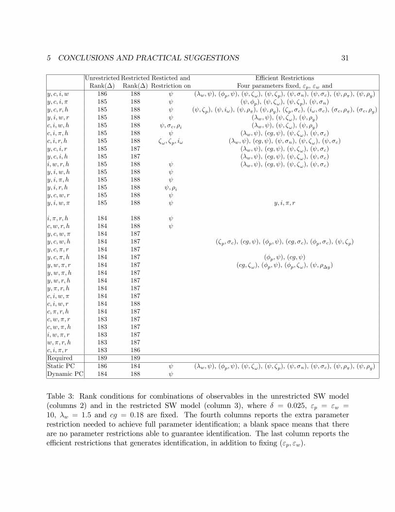
3.1 The results of the rank analysis
The model features 29 parameters, 12 predetermined states and four structural shocks.
Thus, the condition for identi�cation of all structural parameters is that the rank of
�(�0) is equal to 189. We start with an unrestricted speci�cation and ask whether
there exists four dimensional vectors that ensure full identi�ability and, if not, what
combination gets �closest�to meet the rank condition. The number of combinations of
3 AN APPLICATION 13
four observables out of a pool of seven endogenous controls is�74
�= 7!
4!(7�4)! = 35.
The �rst column of table 3 presents a subset of the 35 combinations and the second
column the rank of �j(�0). Clearly, no combination guarantees full parameter identi-
�cation. Hence, our rank analysis con�rms a well known result (see e.g. Iskrev, 2010,
Komunjer and Ng, 2011, Tkachenko and Qu, 2012) that the parameter vector of the
SW model is not identi�able. Interestingly, the combination containing (y; c; i; w), has
the largest rank, 186. Moreover, among the 15 combinations with largest rank, invest-
ment appears in 13 of them. Thus, the dynamics of investment are well identi�ed and
this variable contains useful identi�cation information for the structural parameters.
Conversely, real wages appears often in low rank combinations suggesting that this
variable has relatively low identi�cation power. Among the large rank combinations
the nominal interest rate appears more often than in�ation (7 vs. 4). More striking is
the result that identi�cation is poor when both in�ation and interest rate are among
the observables; indeed, all combinations featuring these two variables are in the low
rank region and four have the lowest rank.
The third column of table 3 repeats the exercise calibrating some of the structural
parameters. It is well known that certain parameters cannot be identi�ed from the
dynamics of the model (e.g. average government expenditure to output ratio) and oth-
ers are implicitly selected by statistical agencies (e.g. the depreciation rate of capital).
Thus, we �x the depreciation rate, � = 0:025, the good markets and labor market
aggregators, "p = "w = 10, elasticity of substitution labor, �w = 1:5; and govern-
ment consumption share in output cg = 0:18, as in SW (2007). Even with these �ve
restrictions, the remaining 24 parameters of the model fail to be identi�ed for any com-
bination of the observable variables. While these �ve restrictions are necessary to make
the mapping from the deep parameters to the reduced form parameters invertible, i.e.
rank(��(�0)) = n� � 5 = 24, they are not su¢ cient to guarantee local identi�cation.Note that the ordering obtained in the unrestricted case is preserved, but di¤erent
combinations of variables have now more similar ranks.
Finally, we examine whether there are parameter restrictions that allow some non-
singular system to identify the remaining vector of parameters. We proceed in two
steps. First, we consider adding one parameter restriction to the �ve restrictions used
in column 3. We report in column 4 the restriction that generates identi�cation for
3 AN APPLICATION 14
each combination of observables. A blank space means that there are no parameter
restrictions able to generate full parameter identi�cation for that combination of ob-
servables. Second, we consider whether �any� set of parameter restrictions generate
full identi�cation; that is, we search for an �e¢ cient�set of restrictions, where by e¢ -
cient we mean a combination of four observables that generates identi�cation with a
minimum number of restrictions. The �fth column of table 3 reports the parameters
restrictions that achieve identi�cation for each combination of observables.
From column 4 one can see that an extra restriction is not enough to achieve full
parameter identi�cation in all cases. In addition, the combinations of variables which
were best in the unrestricted calculation are still those with the largest rank in this
case. Thus, when the SW restrictions are used and an extra restriction is added, large
rank combination generate identi�cation, while for low rank combinations one extra
restriction is insu¢ cient. Interestingly, for most combinations of observables, the para-
meter that has to be �xed is elasticity of capital utilization adjustment costs. Column
5 indicates that at least four restrictions are need to identify the vector of structural
parameters and that the goods and labor market aggregators, "p and "w, cannot be
estimated either individually or jointly for any combination of observables. Thus, the
largest (unrestricted) rank combinations are more likely to produce identi�cation with
a tailored use of parameter restrictions.
The �rst four static principal components of the seven variables track very closely
the (y; c; i; w) combination and e¢ cient identi�cation requires the same restrictions.
Dynamic principal components appear to be poorer and they seem to span the space
of lower rank combinations. Thus, for this system, there seems to be little gain in using
principal components rather than observable variables.
3.2 The results of the elasticity analysis
As mentioned, the rank analysis is unsuited to detect weak and partial identi�cation
problems that often plague the estimation of the structural parameters of the DSGE
model. To investigate potential weak and partial identi�cation issues we compute
the curvature of the convoluted likelihood function of the singular and non-singular
systems and examine whether there are combinations of observables which have good
rank properties and also avoid �atness and ridges in the likelihood function.
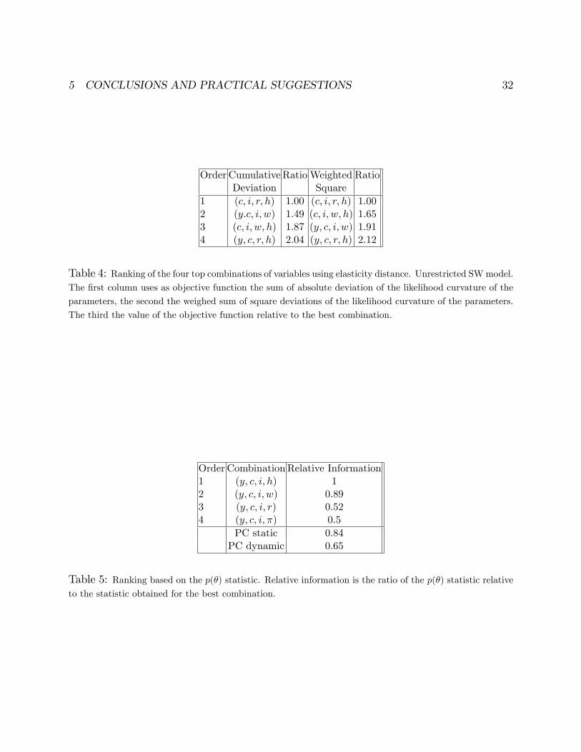
Table 4 presents the four best combinations minimizing the �elasticity�distance.

3 AN APPLICATION 15
We focus attention on six parameters, which are often the object of discussion among
macroeconomists: the habit persistence, the inverse of the Frisch elasticity of labor
supply, the price stickiness and the price indexation parameters, the in�ation and
output coe¢ cients in the Taylor rule. Notice �rst, that the format of the objective
function is irrelevant: the top combinations are also the best according to the second
criterion. Also, by comparing tables 3 and table 4, it is clear that maximizing the
rank of �j(�0) does not necessarily make the curvature of the convoluted likelihood
in the singular and non-singular system close in these six dimensions. The vector of
variables which is best according to the �elasticity�criterion (consumption, investment,
hours and the nominal interest rate) was in the second group in table 3 but the top
combination in that table ranks close second. In general, the presence of the nominal
interest rate helps to identify the habit persistence and the price stickiness parameters;
excluding the nominal rate and hours in favor of output and the real wage (the second
best combination) helps to better identify the price indexation parameter at the cost
of making the identi�ability of the Frisch elasticity worse. Interestingly even the best
combination of variables makes the curvature of likelihood quite �at, for example, in
the dimension represented by the in�ation coe¢ cient in the Taylor rule. Thus, while
there does not exist a combination which simultaneously avoids weak identi�cation in
all six parameters, di¤erent combinations of observables may reduce the extent of the
problem in certain parameters. Hence, depending on the focus of the investigation,
researchers may be justi�ed in using di¤erent vectors of the observables to estimate
the structural parameters.
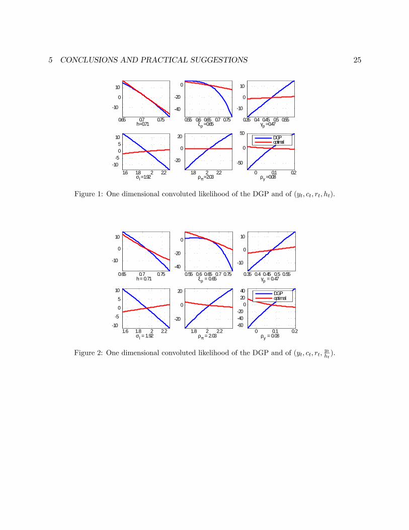
It is worth also mentioning that while there are no theoretical reasons to prefer
any two variables among output, hours and labor productivity, and the ordering the
best models is una¤ected in the rank analysis, there are important weak identi�cation
trade-o¤s in selecting a group of variables or the other. For example, comparing �gures
1 and 2, one can see that if labor productivity is used in place of hours, the �atness of
the likelihood function in the dimensions represented by the in�ation and the output
coe¢ cients in the Taylor rule is reduced, at the cost of worsening the identi�cation
properties of the habit persistence and the price stickiness parameters.

3 AN APPLICATION 16
3.3 The results of the information analysis
Table 5 gives the best combinations of observables according to the information statistic
(11). As in table 4, we also provide the value of the average objective function for that
combination relative to the best.
An econometrician interested in estimating the structural parameters of this model
should de�nitely use output, consumption and investment as observables - they appear
in all four top combinations. The fourth observable seems to be either hours or real
wages, while combinations which include interest rates or in�ation fare quite poorly in
terms of relative informativeness. In general, the performance of alternative combina-
tions deteriorates substantially as we move down in the ordering, suggesting that the
information measure can sharply distinguish various options.
Interestingly, the identi�cation and the informational analyses broadly coincide in
the ordering of vectors of observables: the top combination obtained with the rank
analysis (y; c; i; w) fares second in the information analysis and either second or third
in the elasticity analysis. Moreover, three of the four top combinations in table 5 are
also among the top combinations in table 3. Finally, note that also in this case the
performance of the �rst four static principal components is very similar to the one of
the (y; c; i; w) vector and that dynamic principal components appear to be inferior to
their static counterparts.
3.4 Summary
To estimate the structural parameters of this model it is necessary to include at least
three real variables and output, consumption and investment seem the best for this
purpose. The fourth variable varies according to the criteria. Despite the monetary
nature of this model, jointly including in�ation and the nominal rate among the observ-
ables make things worse. We can think of two reasons for this outcome. First, because
the model features a Taylor rule for monetary policy, in�ation and the nominal rate
tend to comove quite a lot. Second, since the parameters entering the Phillips curve
are di¢ cult to identify no matter what variables are employed, the use of real variables
at least allows us to pin down intertemporal and intratemporal links, which crucially
determine income and substitution e¤ects present in the economy.
As the on-line appendix shows, changes in nuisance parameters present in the two

4 HOW DIFFERENT ARE THE SPECIFICATIONS? 17
procedures, in the sample size, in the choice of shocks of entering the model and in the
speci�cations of the informational distance do not a¤ect these results.
4 How di¤erent are the speci�cations?
To study how di¤erent the �best�and the �worst�speci�cations are in practice, we
generate 150 data points for output (y), consumption (c), investment (i), wages (w),
hours worked (h), in�ation (�) and interest rate (r) using the SW model driven by
four structural shocks (�at ; �it; �
gt ; �
mt ) and parameters as in table 2. We then estimate
the structural parameters of the following �ve models:
� Model A: Four structural shocks and (y; c; i; w) as observables (this is the bestcombination of variables according to the rank analysis).
� Model B: Four structural shocks and (y; c; i; h) as observables (this is the bestcombination of variables according to the information analysis).
� Model Z: Four structural shocks and (c; i; �; r) as observables (this the worstcombination of variables according to the rank analysis).
� Model C: Four structural shocks, three measurement errors, attached to output,interest rates and hours and all seven observable variables.
� Model D: Seven structural shocks - the four basic ones plus price markup, wagemarkup and preference shocks, all assumed to be iid - and all seven observable
variables
and compute responses to interesting shocks. We want to see i) how the best
models (A and B) fare relative to the DGP and to the worst model (Z); ii) how standard
alternatives augmenting the true set of shocks with either arti�cial measurement errors
(C) or with arti�cial structural errors (D), fare in comparison to the best models and
the DGP. In ii) we are particularly interested in whether the presence of three arti�cial
shocks distorts the responses to true disturbances and in whether responses to these
arti�cial shocks display patterns that could lead investigators to confuse them with the
structural disturbances.
The likelihood of the simulated sample is combined with the prior distribution
of the parameters to obtain the posterior distribution in each case. The choice of

4 HOW DIFFERENT ARE THE SPECIFICATIONS? 18
priors closely follows SW(2007) and posterior distributions are obtained using two
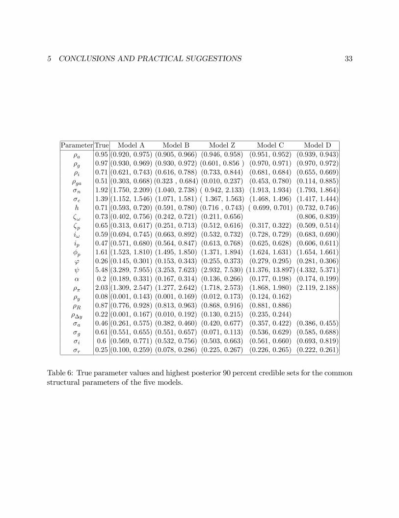
independent chains of 100,000 draws using the MH algorithm. Table 6 presents the
true parameter values and the vector of highest posterior 90 % credible sets for the
�ve models. For model A,B and Z 23 structural parameters are estimated. For model
C; we estimate 22 structural parameters (the wage stickyness parameters is kept �xed)
and the standard deviation of the three measurement errors; for model D we estimate
20 structural parameters (i.e. the monetary policy coe¢ cients are set to their true
values) and the standard deviation of the arti�cial preference, the price and the wage
markups shocks 5.
The table con�rms that models A and B are di¤erent from model Z. Even if
the three models are all correctly speci�ed in terms of structure, there are sizable
di¤erences in the magnitude and the precision of credible sets. In models where the
observables feature large spectral ranks or high information, estimates of the structural
parameters are typically more accurate. For example, in Models A and B there are
four credible sets that do not include the true parameter values, while in model Z
nine credible sets fail to include the true parameter values. In addition, in model Z
important objects, such as the price stickiness and the price indexation parameters,
which crucially determine the slope of the price Phillips curve, are poorly estimated.
It is worth mentioning that in model Z, which uses (c; i; �; r) as observables in
estimation, the government process is very poorly estimated: both the autoregressive
coe¢ cient and the standard deviation of the process are underestimated. One reason for
this outcome is that, in the DGP, gt enters only in the feasibility constraint. In model Z
we only have information about ct and it, which is insu¢ cient to precisely disentangle
gt from yt. This misspeci�cation has important consequences for the transmission of
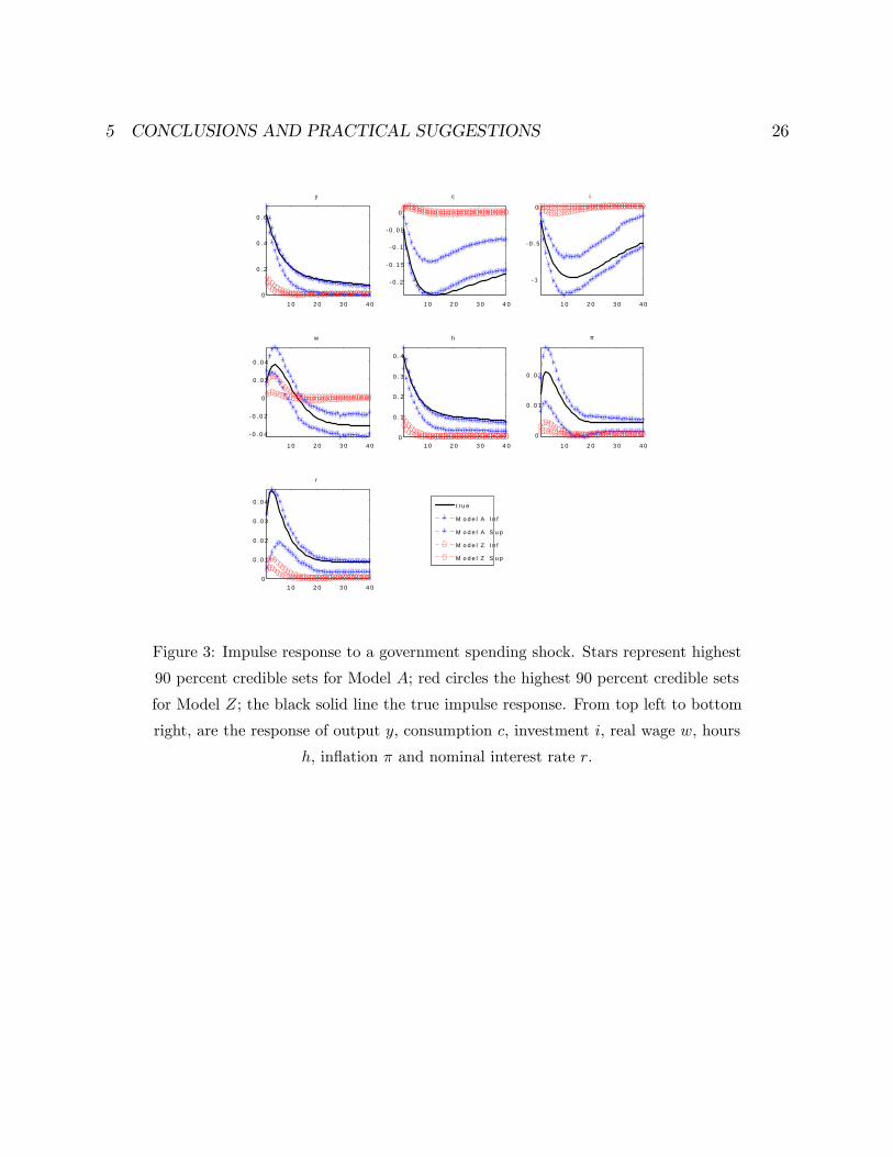
government expenditure shocks. Figure 3 displays the responses of the seven variables
to a positive spending impulse. Stars represent the 90 percent credible sets in Model
A, red circles the 90 percent credible sets of Model Z and the black solid line the
true responses. While Model A correctly identi�es the propagation mechanism of a
spending shock, in the model Z the shock has almost no impact on the variables and
the true response is never contained in the credible sets we present.
5We �x some of the parameters at the true values in models C and D since they turned out to be poorlyidenti�ed and the MCMC routine encountered numerical di¢ culties.

4 HOW DIFFERENT ARE THE SPECIFICATIONS? 19
Estimates of the parameters of models C and D are characterized by di¤erent
degrees of misspeci�cation. In model C, we have added (non-existent) measurement
error to output, hours worked and the nominal interest rate. Since measurement error
is iid and the structural model is correctly speci�ed, one would expect this addition not
to make a huge di¤erence in terms of parameter estimates. In model D, we have added
white noise structural shocks to the dynamics of the original data generating process.
While the shocks that perturb the price Phillips curve, the wage Phillips curve and the
Euler equation are iid, the structure we estimate is misspeci�ed, making estimates of
the structural parameters potentially biased.
Table 6 suggests that distortions are present in both setups but larger in model D.
For example, the posterior sets do not include the true parameters in 13 out of 22 cases
for model C; in 14 out of 20 cases in model D. Furthermore, posterior credible sets are
tight thus incorrectly attributing large informational content to the likelihood. Hence,
augmenting the original model with measurement or structural shocks to employ more
variables in estimation, does not seem to help to produce more accurate estimates of
the structural parameters.
Why are there distortions? First, while the estimated standard deviation of the
three additional shocks is low compared to the standard deviation of the original shocks,
it is a-posteriori di¤erent from zero. Thus, while the estimation procedure recognizes
that these shocks have smaller importance relative to the four original shocks, it wants
to give them a role because the prior heavily penalizes their non-existence. Second, the
signi�cance of arti�cial shocks implies that the properties of other shocks are misspec-
i�ed. For example, in model C, the standard deviation of the technology disturbance
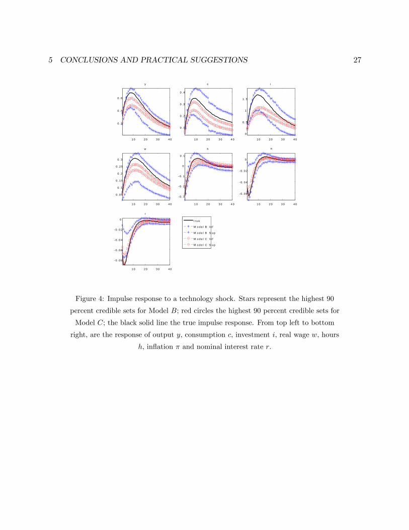
is underestimated. Figure 4, which presents the responses to a technology shock in
the true model (black line) and the highest 90 percent credible sets in Model B (blue
stars) and C (red circles), shows that also the transmission mechanism is altered.
The situation is worse when the estimated model features structural shocks that the
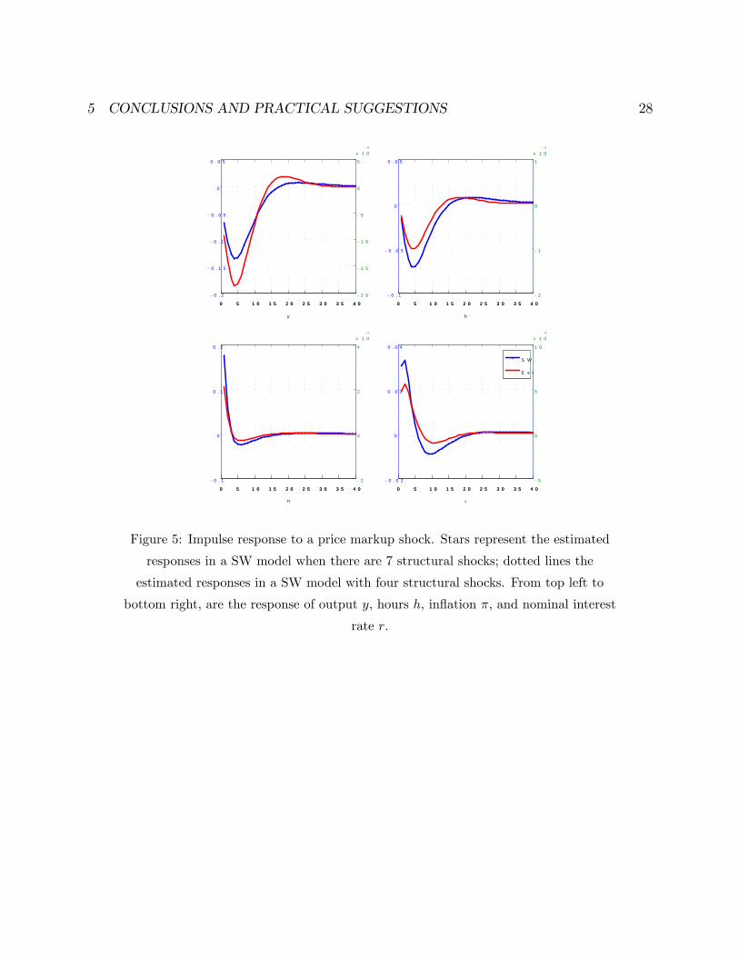
true model does not possess. Figure 5 gives a glimpse of what may happen in this case.
First, notice that the responses of the variables of the system to a (non-existent) price
markup shock are small but a-posteriori signi�cant. Second, the responses have the
same shape (but di¤erent magnitude) as those that would be estimated in case price
markup shocks were truly a part of the DGP (compare dotted and solid lines). Thus, it
is possible to obtain perfectly reasonable patterns of responses even though the shocks

5 CONCLUSIONS AND PRACTICAL SUGGESTIONS 20
which are supposed to drive them are not present in the DGP and the patterns look
very much like those one would obtain if the shocks where present. This conclusion
holds also for the other two shocks, which we have erroneously added in Model D.
Finally, we would like to mention that despite the fact that neither Model A nor
Model B uses any nominal variables in estimation, the responses to a monetary shocks
produced by these model match very well those of the DGP (see on-line appendix).
Hence, we con�rm that capturing the intertemporal and the intratemporal links present
in the model is enough to have the dynamics of the endogenous variables in response
to all the shocks are also well captured.
Overall, it seems a bad idea to add measurement errors to the model to be able
to use more variables in the estimation. Relative to a setup where a reduced num-
ber of variables is chosen in some meaningful way, impulse responses are tighter but
strictly more inaccurate. Similarly, it seems far from optimal to complete the probabil-
ity space of the model by arti�cially inserting structural shocks. Given standard prior
restrictions, their presence will distort parameter estimates and impulse responses in
two ways: they will take away importance from the true shocks; they will have re-
sponses which will look reasonable even if their true e¤ects are zero. In this sense, our
conclusions echo results derived by Cooley and Dweyer (1998) in a di¤erent framework.
To conclude, we would like to mention that the results obtained in this section
are conditional on one particular vector of time series generated by the model. To
check whether the conclusions hold when sampling uncertainty is taken into account,
we have conducted also a small Monte Carlo exercise where for each model estimation
is repeated on 50 di¤erent samples and credible sets are constructed using 90 percent
of the posterior median estimates. Results are unchanged.
5 Conclusions and practical suggestions
This paper proposes criteria to select the observable variables to be used in the esti-
mation of the structural parameters when one feels uncomfortable in having a model
driven by a large number of potentially non-structural shocks or does not have good
reasons to add measurement errors to the decision rules, and insists in working with
a singular DSGE model. The methods we suggest measure the identi�cation and the
information content of vectors of observables, are easy to implement, and seem able

5 CONCLUSIONS AND PRACTICAL SUGGESTIONS 21
to e¤ectively rank combinations of variables. Interestingly, and despite the fact that
the statistics we employ are derived from di¤erent principles, the best combinations of
variables these methods deliver are pretty much the same.
In the model we consider, parameter identi�cation and variable informativeness
are optimized including output, consumption and investment among the observables.
These variables help to identify the intertemporal and the intratemporal links in the
model and thus are useful to correctly measure income and substitution e¤ects, which
crucially determine the dynamics of the model in response to the shocks. Interestingly,
using interest rate and in�ation jointly in the estimation makes identi�cation worse and
the loss of information due to variable reduction larger. When one takes the curvature
of the likelihood into consideration, the nominal interest rate is weakly preferable to
the in�ation rate.
We also show that, in terms of likelihood curvature, there are important trade-
o¤s when deciding to use hours or labor productivity together with output among the
observables and demonstrate that changes in the setup of the experiment do not alter
the main conclusions of the exercise.
The estimation exercise we perform indicates that the best models our criteria
select capture the conditional dynamics of the singular model reasonably well while
the worst models do not. Furthermore, the practice of tagging-on measurement errors
or non-existent structural shocks to use a larger number of observables in estimation
may distort parameter estimates and jeopardize inference.
While our conclusions are sharp, an econometrician working in a real world appli-
cation should certainly consider whether the measurement of a variables is reliable or
not. Our study only asks what set of observables is preferable, when a singular model
is assumed to be the DGP. In practice, the analysis can be undertaken also when some
justi�ed measurement error is preliminarily added to the model.
In designing criteria to select the variables for estimation, we have taken as given
that researchers have a set of shocks they are interested in studying. One may also
consider the alternative of a researcher with no strong a-priori ideas about which dis-
turbances the theory should specify. In this case, our variable selection procedures can
be nested in a more general approach which would involve taking a vector of data,
characterizing the principal components of the one-step ahead prediction error and se-
lecting those explaining a certain prespeci�ed variance of the data (as in Andrle, 2012).
5 CONCLUSIONS AND PRACTICAL SUGGESTIONS 22
Then, one would perform prior predictive analysis to select the theoretical shocks that
are more likely to generate the second order properties produced in the data by the
principal components of the shocks one has selected. Once this is done, our procedures
can then be applied to select the endogenous variables used for estimation, given the
empirically selected vector of structural shocks.
Our selection criteria implicitly assume that all variables are equally relevant from
an economic point of view. That may not always be the case and one may have a set
of core variables and a set of ancillary variables, potentially relevant to characterize
a phenomena. For example, in a model featuring macro-�nancial linkages, the macro
variables could be held �xed and one may want to choose the vector of �nancial vari-
ables that best inform researchers on this link. In this situation, our selection criteria
can be used to select relevant variables from the latter set.
The approaches are designed with the idea that a researcher wants to use the
likelihood function for inferential purposes. If this is not the case, the spectral methods
of Qu and Tkachenko (2011) can be employed to estimate the structural parameters,
since the spectral density is well de�ned object that can be optimized, even in a singular
system.
One way of interpreting our exercises is in terms of prior predictive analysis (see
Faust and Gupta, 2011). In this perspective, prior to the estimation of the structural
parameters, one may want to examine which features of the model are well identi�ed
and what is the information content of di¤erent vector of observables. Seen through
these lenses, the analysis we perform complements those of Canova and Paustian (2011)
and of Mueller (2010).
References
An, S. and Schorfheide, F. , 2007. Bayesian analysis of DSGE models. Econometric
Reviews, 26, 113-172.
Andrle, M., 2012. Estimating DSGE models using likelihood based dimensionality
reduction. IMF manuscript.
Bierens, H., 2007. Econometric analysis of linearized DSGE models. Journal of
Econometrics, 136, 595-627.
Canova, F. and Sala, L., 2009. Back to square one: identi�cation issues in DSGE
5 CONCLUSIONS AND PRACTICAL SUGGESTIONS 23
models. Journal of Monetary Economics, 56, 431-449.
Canova, F. and Paustian, M., 2011. Business cycle measurement with some theory.
Journal of Monetary Economics, 58, 345-361.
Chari, V.V., Kehoe, P. and McGrattan, E., 2009. New keynesian models: Not yet
useful for policy analyses. American Economic Journals: Macroeconomics, 1, 242-266.
Chang, Y. , S. Kim and Schorfheide, F., 2013. Labor market heterogeneity and the
Lucas critique, Journal of the European Economic Association, 11, 193-220.
Cochrane, J., 2011. Determinacy and identi�cation of Taylor rules. Journal of
Political Economy, 119, 565-615.
Cooley, T. and Dweyer, M., 1989. Business cycle analysis without too much theory:
A look at structural VARs. Journal of Econometrics, 83, 57-88.
Del Negro, M. and Schorfheide, F., forthcoming. DSGE model-based forecasting,
Handbook of Economic Forecasting, volume 2.
Faust, J., and Gupta, A. , 2011. Posterior predictive analysis for evaluating DSGE
models. John Hopkins University manuscript.
Guerron Quintana, P. , 2010. What do you match does matter: the e¤ects of data
on DSGE estimation. Journal of Applied Econometrics, 25, 774-804.
Kascha, C. and Mertens, K., 2010. Business cycle analysis and VARMA. Journal
of Economic Dynamics and Control, 33, 267-282.
Kleibergen, F. and Mavroedis, S., 2009. Weak instrument robust tests in GMM
and the New Keynesian Phillips curve. Journal of Business and Economic Statistics,
27, 293-311.
Komunjer, I. and Ng, S., 2011 Dynamic identi�cation of DSGE models. Economet-
rica, 79, 1995-2032.
Iskrev, N., 2010. Local identi�cation in DSGE Models. Journal of Monetary Eco-
nomics, 57, 189-202.
Mavroedis, S., 2005. Identi�cation issues in forward looking models estimated by
GMM with an application to the Phillips curve. Journal of Money, Credit and Banking,
37, 421-448.
Mueller, U., 2010. Measuring prior sensitivity and prior informativeness in large
Bayesian models. Princeton University manuscript.
Qu, Z. and Tkachenko, D., 2012. Identi�cation and frequency domain QML esti-
mation of linearized DSGE models. Quantitative Economics, 3, 95-132.

5 CONCLUSIONS AND PRACTICAL SUGGESTIONS 24
Sala, L., Soderstrom, U., and Trigari, A., 2010. Output gap, the labor wedge, and
the dynamic behavior of hours. IGIER working paper.
Smets, F. and Wouters, R., 2007. Shocks and frictions in US business cycles: a
Bayesian approach. American Economic Review, 97, 586-606.
5 CONCLUSIONS AND PRACTICAL SUGGESTIONS 25
0.65 0.7 0.75
10
0
10
h = 0.710.55 0.6 0.65 0.7 0.75
40
20
0
ξp = 0.650.35 0.4 0.45 0.5 0.55
10
0
10
γp = 0.47
1.6 1.8 2 2.210
505
10
σl = 1.921.8 2 2.2
20
0
20
ρπ = 2.030 0.1 0.2
50
0
50
ρy = 0.08
DGPoptimal
Figure 1: One dimensional convoluted likelihood of the DGP and of (yt; ct; rt; ht).
0.65 0.7 0.75
10
0
10
h = 0.710.55 0.6 0.65 0.7 0.75
40
20
0
ξp = 0.650.35 0.4 0.45 0.5 0.55
10
0
10
γp = 0.47
1.6 1.8 2 2.210
5
0
5
10
σl = 1.921.8 2 2.2
20
0
20
ρπ = 2.030 0.1 0.2
604020
02040
ρy = 0.08
DGPoptimal
Figure 2: One dimensional convoluted likelihood of the DGP and of (yt; ct; rt;ytht).
5 CONCLUSIONS AND PRACTICAL SUGGESTIONS 26
1 0 2 0 3 0 4 00
0 . 2
0 . 4
0 . 6
y
1 0 2 0 3 0 4 0
0 . 2
0 . 1 5
0 . 1
0 . 0 5
0
c
1 0 2 0 3 0 4 0
1
0 . 5
0
i
1 0 2 0 3 0 4 0
0 . 0 4
0 . 0 2
0
0 . 0 2
0 . 0 4
w
1 0 2 0 3 0 4 00
0 . 1
0 . 2
0 . 3
0 . 4
h
1 0 2 0 3 0 4 0
0
0 . 0 1
0 . 0 2
π
1 0 2 0 3 0 4 00
0 . 0 1
0 . 0 2
0 . 0 3
0 . 0 4
r
t r u e
M o d e l A I n f
M o d e l A S u p
M o d e l Z I n f
M o d e l Z S u p
Figure 3: Impulse response to a government spending shock. Stars represent highest
90 percent credible sets for Model A; red circles the highest 90 percent credible sets
for Model Z; the black solid line the true impulse response. From top left to bottom
right, are the response of output y, consumption c, investment i, real wage w, hours
h, in�ation � and nominal interest rate r.
5 CONCLUSIONS AND PRACTICAL SUGGESTIONS 27
1 0 2 0 3 0 4 0
0 . 2
0 . 4
0 . 6
y
1 0 2 0 3 0 4 0
0 . 1
0 . 2
0 . 3
0 . 4
c
1 0 2 0 3 0 4 0
0
0 . 5
1
1 . 5
i
1 0 2 0 3 0 4 0
0 . 0 5
0 . 1
0 . 1 5
0 . 2
0 . 2 5
0 . 3
w
1 0 2 0 3 0 4 0
0 . 3
0 . 2
0 . 1
0
0 . 1
h
1 0 2 0 3 0 4 0
0 . 0 6
0 . 0 4
0 . 0 2
0
π
1 0 2 0 3 0 4 0
0 . 0 8
0 . 0 6
0 . 0 4
0 . 0 2
0
r
t ru e
M o d e l B I n f
M o d e l B S u p
M o d e l C I n f
M o d e l C S u p
Figure 4: Impulse response to a technology shock. Stars represent the highest 90
percent credible sets for Model B; red circles the highest 90 percent credible sets for
Model C; the black solid line the true impulse response. From top left to bottom
right, are the response of output y, consumption c, investment i, real wage w, hours
h, in�ation � and nominal interest rate r.
5 CONCLUSIONS AND PRACTICAL SUGGESTIONS 28
0 5 1 0 1 5 2 0 2 5 3 0 3 5 4 0
0 . 2
0 . 1 5
0 . 1
0 . 0 5
0
0 . 0 5
y
0 5 1 0 1 5 2 0 2 5 3 0 3 5 4 0
2 0
1 5
1 0
5
0
5
x 1 0 4
0 5 1 0 1 5 2 0 2 5 3 0 3 5 4 0
0 . 1
0 . 0 5
0
0 . 0 5
h
0 5 1 0 1 5 2 0 2 5 3 0 3 5 4 0
2
1
0
1
x 1 0 3
0 5 1 0 1 5 2 0 2 5 3 0 3 5 4 0
0 . 1
0
0 . 1
0 . 2
π
0 5 1 0 1 5 2 0 2 5 3 0 3 5 4 0
2
0
2
4
x 1 0 3
0 5 1 0 1 5 2 0 2 5 3 0 3 5 4 0
0 . 0 2
0
0 . 0 2
0 . 0 4
r
0 5 1 0 1 5 2 0 2 5 3 0 3 5 4 0
5
0
5
1 0
x 1 0 4
S W
E s t
Figure 5: Impulse response to a price markup shock. Stars represent the estimated
responses in a SW model when there are 7 structural shocks; dotted lines the
estimated responses in a SW model with four structural shocks. From top left to
bottom right, are the response of output y, hours h, in�ation �, and nominal interest
rate r.
5 CONCLUSIONS AND PRACTICAL SUGGESTIONS 29
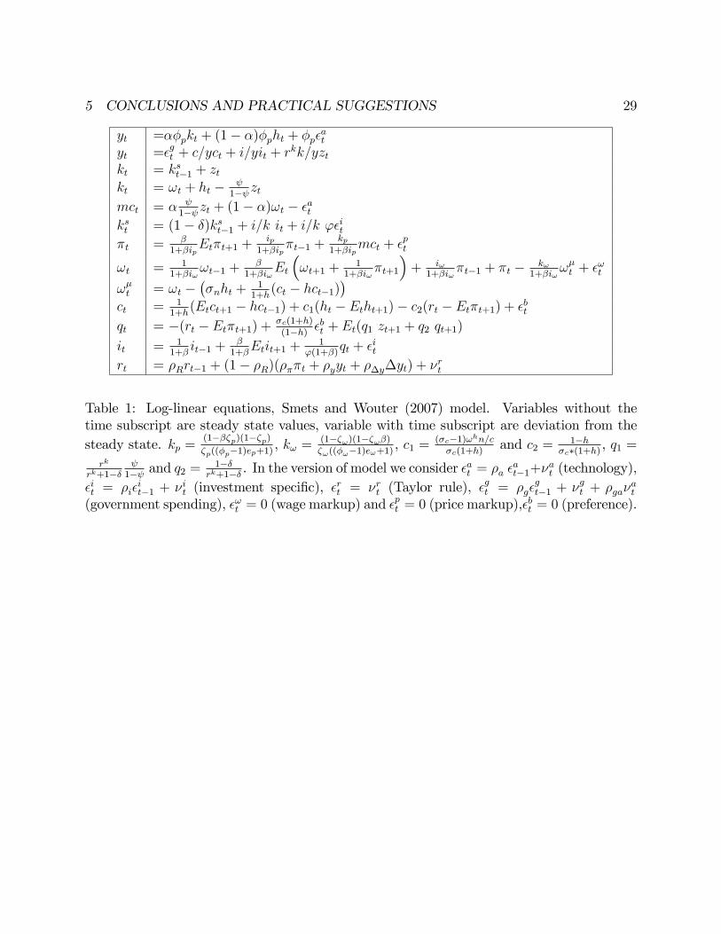
yt =��pkt + (1� �)�pht + �p�at
yt =�gt + c=yct + i=yit + rkk=yztkt = kst�1 + ztkt = !t + ht �
1� ztmct = �
1� zt + (1� �)!t � �atkst = (1� �)kst�1 + i=k it + i=k '�it�t = �
1+�ipEt�t+1 +
ip1+�ip
�t�1 +kp
1+�ipmct + �pt
!t = 11+�i!
!t�1 +�
1+�i!Et
�!t+1 +
11+�i!
�t+1
�+ i!
1+�i!�t�1 + �t � k!
1+�i!!�t + �!t
!�t = !t ���nht +
11+h(ct � hct�1)
�ct = 1
1+h(Etct+1 � hct�1) + c1(ht � Etht+1)� c2(rt � Et�t+1) + �bt
qt = �(rt � Et�t+1) +�c(1+h)(1�h) �
bt + Et(q1 zt+1 + q2 qt+1)
it = 11+�
it�1 +�1+�
Etit+1 +1
'(1+�)qt + �it
rt = �Rrt�1 + (1� �R)(���t + �yyt + ��y�yt) + �rt
Table 1: Log-linear equations, Smets and Wouter (2007) model. Variables without thetime subscript are steady state values, variable with time subscript are deviation from thesteady state. kp =
(1���p)(1��p)�p((�p�1)ep+1)
, k! =(1��!)(1��!�)�!((�!�1)e!+1)
, c1 =(�c�1)!hn=c�c(1+h)
and c2 = 1�h�c�(1+h) , q1 =
rk
rk+1�� 1� and q2 =
1��rk+1�� . In the version of model we consider �
at = �a �
at�1+�
at (technology),
�it = �i�it�1 + �it (investment speci�c), �
rt = �rt (Taylor rule), �
gt = �g�
gt�1 + �gt + �ga�
at
(government spending), �!t = 0 (wage markup) and �pt = 0 (price markup),�
bt = 0 (preference).

5 CONCLUSIONS AND PRACTICAL SUGGESTIONS 30
� Description Value� depreciation rate 0.025"p good markets kimball aggregator 10"w labor markets kimball aggregator 10�w elasticity of substitution labor 1.5cg gov�t consumption output share 0.18� time discount factor 0.998�p 1 plus the share of �xed cost in production 1.61 elasticity capital utilization adjustment costs 5.74� capital share 0.19h habit in consumption 0.71�! wage stickiness 0.73�p price stickiness 0.65i! wage indexation 0.59ip price indexation 0.47�n elasticity of labor supply 1.92�c intertemporal elasticity of substitution 1.39' st. st. elasticity of capital adjustment costs 0.54�� monetary policy response to � 2.04�R monetary policy autoregressive coe¤. 0.81�y monetary policy response to y 0.08��y monetary policy response to y growth 0.22�a technology autoregressive coe¤. 0.95�g gov spending autoregressive coe¤. 0.97�i investment autoregressive coe¤. 0.71�ga cross coe¢ cient tech-gov 0.52�a sd technology 0.45�g sd government spending 0.53�i sd investment 0.45�r sd monetary policy 0.24
Table 2: Parameters description and values used in the DGP.
5 CONCLUSIONS AND PRACTICAL SUGGESTIONS 31
Unrestricted Restricted Resticted and E¢ cient RestrictionsRank(�) Rank(�) Restriction on Four parameters �xed, "p, "w and
y; c; i; w 186 188 (�w; ), (�p; ), ( ; �!), ( ; �p), ( ; �n), ( ; �c), ( ; ��), ( ; �y)y; c; i; � 185 188 ( ; �p), ( ; �!), ( ; �p), ( ; �n)y; c; r; h 185 188 ( ; �p), ( ; i!), ( ; ��), ( ; �y), (�p; �c), (i!; �c), (�c; ��), (�c; �y)y; i; w; r 185 188 (�w; ), ( ; �!), ( ; �y)c; i; w; h 185 188 ; �c; �i (�w; ), ( ; �!), ( ; �y)c; i; �; h 185 188 (�w; ), (cg; ), ( ; �!), ( ; �c)c; i; r; h 185 188 �!; �p; i! (�w; ), (cg; ), ( ; �n), ( ; �!), ( ; �c)y; c; i; r 185 187 (�w; ), (cg; ), ( ; �!), ( ; �c)y; c; i; h 185 187 (�w; ), (cg; ), ( ; �!), ( ; �c)i; w; r; h 185 188 (�w; ), (cg; ), ( ; �!), ( ; �c)y; i; w; h 185 188 y; i; �; h 185 188 y; i; r; h 185 188 ; �iy; c; w; r 185 188 y; i; w; � 185 188 y; i; �; r
i; �; r; h 184 188 c;w; r; h 184 188 y; c; w; � 184 187y; c; w; h 184 187 (�p; �c), (cg; ), (�p; ), (cg; �c), (�p; �c), ( ; �p)y; c; �; r 184 187y; c; �; h 184 187 (�p; ), (cg; )y; w; �; r 184 187 (cg; �!), (�p; ), (�p; �!), ( ; ��y)y; w; �; h 184 187y; w; r; h 184 187y; �; r; h 184 187c; i; w; � 184 187c; i; w; r 184 188c; �; r; h 184 187c; w; �; r 183 187c; w; �; h 183 187i; w; �; r 183 187w; �; r; h 183 187c; i; �; r 183 186Required 189 189Static PC 186 184 (�w; ), (�p; ), ( ; �!), ( ; �p), ( ; �n), ( ; �c), ( ; ��), ( ; �y)Dynamic PC 184 188
Table 3: Rank conditions for combinations of observables in the unrestricted SW model(columns 2) and in the restricted SW model (column 3), where � = 0:025, "p = "w =10, �w = 1:5 and cg = 0:18 are �xed. The fourth columns reports the extra parameterrestriction needed to achieve full parameter identi�cation; a blank space means that thereare no parameter restrictions able to guarantee identi�cation. The last column reports thee¢ cient restrictions that generates identi�cation, in addition to �xing ("p; "w).
5 CONCLUSIONS AND PRACTICAL SUGGESTIONS 32
Order Cumulative Ratio Weighted RatioDeviation Square
1 (c; i; r; h) 1.00 (c; i; r; h) 1.002 (y:c; i; w) 1.49 (c; i; w; h) 1.653 (c; i; w; h) 1.87 (y; c; i; w) 1.914 (y; c; r; h) 2.04 (y; c; r; h) 2.12
Table 4: Ranking of the four top combinations of variables using elasticity distance. Unrestricted SWmodel.
The �rst column uses as objective function the sum of absolute deviation of the likelihood curvature of the
parameters, the second the weighed sum of square deviations of the likelihood curvature of the parameters.
The third the value of the objective function relative to the best combination.
Order CombinationRelative Information1 (y; c; i; h) 12 (y; c; i; w) 0.893 (y; c; i; r) 0.524 (y; c; i; �) 0.5
PC static 0.84PC dynamic 0.65
Table 5: Ranking based on the p(�) statistic. Relative information is the ratio of the p(�) statistic relativeto the statistic obtained for the best combination.
5 CONCLUSIONS AND PRACTICAL SUGGESTIONS 33
Parameter True Model A Model B Model Z Model C Model D�a 0.95 (0.920, 0.975) (0.905, 0.966) (0.946, 0.958) (0.951, 0.952) (0.939, 0.943)�g 0.97 (0.930, 0.969) (0.930, 0.972) (0.601, 0.856 ) (0.970, 0.971) (0.970, 0.972)�i 0.71 (0.621, 0.743) (0.616, 0.788) (0.733, 0.844) (0.681, 0.684) (0.655, 0.669)�ga 0.51 (0.303, 0.668) (0.323 , 0.684) (0.010, 0.237) (0.453, 0.780) (0.114, 0.885)�n 1.92 (1.750, 2.209) (1.040, 2.738) ( 0.942, 2.133) (1.913, 1.934) (1.793, 1.864)�c 1.39 (1.152, 1.546) (1.071, 1.581) ( 1.367, 1.563) (1.468, 1.496) (1.417, 1.444)h 0.71 (0.593, 0.720) (0.591, 0.780) (0.716 , 0.743) ( 0.699, 0.701) (0.732, 0.746)�! 0.73 (0.402, 0.756) (0.242, 0.721) (0.211, 0.656) (0.806, 0.839)�p 0.65 (0.313, 0.617) (0.251, 0.713) (0.512, 0.616) (0.317, 0.322) (0.509, 0.514)i! 0.59 (0.694, 0.745) (0.663, 0.892) (0.532, 0.732) (0.728, 0.729) (0.683, 0.690)ip 0.47 (0.571, 0.680) (0.564, 0.847) (0.613, 0.768) (0.625, 0.628) (0.606, 0.611)�p 1.61 (1.523, 1.810) (1.495, 1.850) (1.371, 1.894) (1.624, 1.631) (1.654, 1.661)' 0.26 (0.145, 0.301) (0.153, 0.343) (0.255, 0.373) (0.279, 0.295) (0.281, 0.306) 5.48 (3.289, 7.955) (3.253, 7.623) (2.932, 7.530) (11.376, 13.897) (4.332, 5.371)� 0.2 (0.189, 0.331) (0.167, 0.314) (0.136, 0.266) (0.177, 0.198) (0.174, 0.199)�� 2.03 (1.309, 2.547) (1.277, 2.642) (1.718, 2.573) (1.868, 1.980) (2.119, 2.188)�y 0.08 (0.001, 0.143) (0.001, 0.169) (0.012, 0.173) (0.124, 0.162)�R 0.87 (0.776, 0.928) (0.813, 0.963) (0.868, 0.916) (0.881, 0.886)��y 0.22 (0.001, 0.167) (0.010, 0.192) (0.130, 0.215) (0.235, 0.244)�a 0.46 (0.261, 0.575) (0.382, 0.460) (0.420, 0.677) (0.357, 0.422) (0.386, 0.455)�g 0.61 (0.551, 0.655) (0.551, 0.657) (0.071, 0.113) (0.536, 0.629) (0.585, 0.688)�i 0.6 (0.569, 0.771) (0.532, 0.756) (0.503, 0.663) (0.561, 0.660) (0.693, 0.819)�r 0.25 (0.100, 0.259) (0.078, 0.286) (0.225, 0.267) (0.226, 0.265) (0.222, 0.261)
Table 6: True parameter values and highest posterior 90 percent credible sets for the commonstructural parameters of the �ve models.