Embed Size (px)
Citation preview
Multivariate Behavioral Research, 48:28–56, 2013
Copyright © Taylor & Francis Group, LLC
ISSN: 0027-3171 print/1532-7906 online
DOI: 10.1080/00273171.2012.710386
Choosing the Optimal Number ofFactors in Exploratory Factor Analysis:
A Model Selection Perspective
Kristopher J. PreacherVanderbilt University
Guangjian ZhangUniversity of Notre Dame
Cheongtag KimSeoul National University
Gerhard MelsScientific Software International
A central problem in the application of exploratory factor analysis is deciding how
many factors to retain (m). Although this is inherently a model selection problem, a
model selection perspective is rarely adopted for this task. We suggest that Cudeck
and Henly’s (1991) framework can be applied to guide the selection process.
Researchers must first identify the analytic goal: identifying the (approximately)
correct m or identifying the most replicable m. Second, researchers must choose fit
indices that are most congruent with their goal. Consistent with theory, a simulation
study showed that different fit indices are best suited to different goals. Moreover,
model selection with one goal in mind (e.g., identifying the approximately correct
m) will not necessarily lead to the same number of factors as model selection with
the other goal in mind (e.g., identifying the most replicable m). We recommend
that researchers more thoroughly consider what they mean by “the right number
of factors” before they choose fit indices.
Correspondence concerning this article should be addressed to Kristopher J. Preacher, Psychology
& Human Development, Vanderbilt University, PMB 552, 230 Appleton Place, Nashville, TN 37203-
5721. E-mail: [email protected]
28
Dow
nloa
ded
by [
VU
L V
ande
rbilt
Uni
vers
ity]
at 1
6:24
29
Mar
ch 2
013
MODEL SELECTION IN FACTOR ANALYSIS 29
Exploratory factor analysis (EFA) is a method of determining the number and
nature of unobserved latent variables that can be used to explain the shared
variability in a set of observed indicators, and is one of the most valuable
methods in the statistical toolbox of social science. A recurring problem in the
practice of EFA is that of deciding how many factors to retain. Numerous prior
studies have shown that retaining too few or too many factors can have dire
consequences for the interpretation and stability of factor patterns, so choosing
the optimal number of factors has, historically, represented a crucially important
decision. The number-of-factors problem has been described as “one of the
thorniest problems a researcher faces” (Hubbard & Allen, 1989, p. 155) and
as “likely to be the most important decision a researcher will make” (Zwick &
Velicer, 1986, p. 432). Curiously, although this is inherently a model selection
problem, a model selection perspective is rarely adopted for this task.
Model selection is the practice of selecting from among a set of competing
theoretical explanations the model that best balances the desirable characteristics
of parsimony and fit to observed data (Myung & Pitt, 1998). Our threefold
goals are to (a) suggest that a model selection approach be taken with respect to
determining the number of factors, (b) suggest a theoretical framework to help
guide the decision process, and (c) contrast the performance of several competing
criteria for choosing the optimal number of factors within this framework.
First, we offer a brief overview of EFA and orient the reader to the nature
of the problem of selecting the optimal number of factors. Next, we describe
several key issues critical to the process of model selection. We employ a
theoretical framework suggested by Cudeck and Henly (1991) to organize issues
relevant to the decision process. Finally, we provide demonstrations (in the
form of simulation studies and application to real data) to highlight how model
selection can be used to choose the number of factors. Most important, we
make the case that identifying the approximately correct number of factors and
identifying the most replicable number of factors represent separate goals, often
with different answers, but that both goals are worthy of, and amenable to,
pursuit.
OVERVIEW OF EXPLORATORY FACTOR ANALYSIS
The Common Factor Model
In EFA, the common factor model is used to represent observed measured
variables (MVs) as functions of model parameters and unobserved factors or
latent variables (LVs). The model for raw data is defined as follows:
x D ƒŸ C •; (1)
Dow
nloa
ded
by [
VU
L V
ande
rbilt
Uni
vers
ity]
at 1
6:24
29
Mar
ch 2
013
30 PREACHER, ZHANG, KIM, MELS
where x is a p�1 vector containing data from a typical individual on p variables,
ƒ is a p � m matrix of factor loadings relating the p variables to m factors, Ÿ
is an m � 1 vector of latent variables, and • is a p � 1 vector of person-specific
scores on unique factors. The • are assumed to be mutually uncorrelated and
uncorrelated with Ÿ. The covariance structure implied by Equation (1) is as
follows:
† D ƒˆƒ0 C ‰; (2)
where † is a p � p population covariance matrix, ƒ is as defined earlier, ˆ
is a symmetric matrix of factor variances and covariances, and ‰ is a diagonal
matrix of unique factor variances. Parameters in ƒ, ˆ, and ‰ are estimated
using information in observed data. The factor loadings in ƒ are usually of
primary interest. However, they are not uniquely identified, so the researcher will
usually select the solution for ƒ that maximizes some criterion of interpretability.
The pattern of high and low factor loadings in this transformed (or rotated) ƒ
identifies groups of variables that are related or that depend on the same common
factors.
A Critical but Subjective Decision in Factor Analysis
In most applications of EFA, of primary interest to the analyst are the m
common factors that account for most of the observed covariation in a data
set. Determination of the number and nature of these factors is the primary
motivation for conducting EFA. Therefore, probably the most critical subjective
decision in factor analysis is the number of factors to retain (i.e., identifying
the dimension of ƒ), the primary focus of this article. We now expand on this
issue.
SELECTING THE OPTIMAL NUMBER OF FACTORS
Although the phrase is used frequently, finding the “correct” or “true” number
of factors is an unfortunate choice of words. The assumption that there exists a
correct, finite number of factors implies that the common factor model has
the potential to perfectly describe the population factor structure. However,
many methodologists (Bentler & Mooijaart, 1989; Cattell, 1966; Cudeck, 1991;
Cudeck & Henly, 1991; MacCallum, 2003; MacCallum & Tucker, 1991; Meehl,
1990) argue that in most circumstances there is no true operating model, re-
gardless of how much the analyst would like to believe such is the case.
The hypothetically true model would likely be infinitely complex and would
completely capture the data-generating process only at the instant at which
Dow
nloa
ded
by [
VU
L V
ande
rbilt
Uni
vers
ity]
at 1
6:24
29
Mar
ch 2
013
MODEL SELECTION IN FACTOR ANALYSIS 31
the data are recorded. MacCallum, Browne, and Cai (2007) further observe
that distributional assumptions are virtually always violated, the relationships
between items and factors are rarely linear, and factor loadings are rarely (if ever)
exactly invariant across individuals. By implication, all models are misspecified,
so the best we can expect from a model is that it provide an approximation
to the data-generating process that is close enough to be useful (Box, 1976).
We agree with Cudeck and Henly (2003) when they state, “If guessing the
true model is the goal of data analysis, the exercise is a failure at the outset”
(p. 380).
Given the perspective that there is no true model, the search for the correct
number of factors in EFA would seem to be a pointless undertaking. First,
if the common factor model is correct in a given setting, it can be argued
that the correct number of factors is at least much larger than the number
of variables (Cattell, 1966) and likely infinite (Humphreys, 1964). For this
reason, Cattell (1966) emphasized that the analyst should consider not the
correct number of factors but rather the number of factors that are worthwhile
to retain. A second plausible argument is that there exists a finite number
of factors (i.e., a true model) but that this number is ultimately unknowable
by psychologists because samples are finite and models inherently lack the
particular combination of complexity and specificity necessary to discover them.
A third perspective is that the question of whether or not there exists a “true
model” is inconsequential because the primary goals of modeling are description
and prediction. Discovering the true model, and therefore the “correct” m, is
unnecessary in service of this third stated goal as long as the retained factors
are adequate for descriptive or predictive purposes.
Given this variety of perspectives, none of which is optimistic about finding
a true m, one might reasonably ask if it is worth the effort to search for the
correct number of factors. We think the search is a worthwhile undertaking, but
the problem as it is usually stated is ill posed. A better question regards not the
true number of factors but rather the optimal number of factors to retain. By
optimal we mean the best number of factors to retain in order to satisfy a given
criterion in service of meeting some explicitly stated scientific goal. One example
of a scientific goal is identifying the model with the highest verisimilitude,
or proximity to the objective truth (Meehl, 1990; Popper, 1959). This goal
stresses accuracy in explanation as the overriding concern while recognizing
that no model can ever fully capture the complexities of the data-generating
process. On the other hand, in many contexts it is more worthwhile to search
for a model that stresses generalizability, or the ability to cross-validate well
to data arising from the same underlying process (Cudeck & Henly, 1991;
Myung, 2000; Pitt & Myung, 2002). This goal stresses prediction or replicability
as fundamentally important. The correct model, in the unlikely event that it
really exists and can be discovered, is of little use if it does not generalize
Dow
nloa
ded
by [
VU
L V
ande
rbilt
Uni
vers
ity]
at 1
6:24
29
Mar
ch 2
013

32 PREACHER, ZHANG, KIM, MELS
to future data or other samples (Everett, 1983; Fabrigar, Wegener, MacCallum,
& Strahan, 1999; Thompson, 1994). A generalizable model, even if it does
not completely capture the actual data-generating process, can nevertheless be
useful in practice.1 In fact, in some contexts, such as the construction of college
admissions instruments or career counseling, the primary purpose of model
construction concerns selection or prediction, and verisimilitude is of secondary
concern.
We consider it safe to claim that the motivation behind most modeling is some
combination of maximizing verisimilitude and maximizing generalizability. The
search for the optimal number of factors in EFA can be conducted in a way
consistent with each of these goals. To meet the first goal, that of maximizing
verisimilitude, the optimal number of factors is that which provides the most
accurate summary of the factor structure underlying the population of inference
(Burnham & Anderson, 2004, term this best approximating model quasi-true,
a term we adopt here). That is, we seek to identify an m such that the model
fits at least reasonably well with m factors, substantially worse with m � 1
factors, and does not fit substantially better with m C 1 factors. To meet the
goal of maximizing generalizability, the optimal number of factors is that which
provides the least error of prediction upon application to future (or parallel)
samples. That is, we seek the model that demonstrates the best cross-validation
upon being fit to a new sample from the same population. Happily, regardless
of the scientist’s goal, the logic of model selection may be used to guide the
choices involved in EFA.
ADOPTING A MODEL SELECTION PERSPECTIVE
Model Selection
We submit that the search for the optimal number of factors should be ap-
proached as a model selection problem guided by theory. The role of theory in
this process should be to determine, a priori, a set of plausible candidate models
(i.e., values of m) that will be compared using observed data. Often, different
theories posit different numbers of factors to account for observed phenomena,
for example, three-factor versus five-factor theories of personality (Costa &
McCrae, 1992; Eysenck, 1991). Even when theory provides little explicit help
in choosing reasonable values for m, scientists rarely use EFA without some
prior idea of the range of values of m it is plausible to entertain.
1Famous examples of incorrect but useful models are Newtonian physics and the Copernican
theory of planetary motion.
Dow
nloa
ded
by [
VU
L V
ande
rbilt
Uni
vers
ity]
at 1
6:24
29
Mar
ch 2
013
MODEL SELECTION IN FACTOR ANALYSIS 33
Earlier we defined model selection as the practice of selecting from among a
set of competing theoretical explanations the model that best balances the desir-
able characteristics of parsimony and fit to observed data (Myung & Pitt, 1998).
The rival models traditionally are compared using objective model selection
criteria (Sclove, 1987). We collectively refer to criteria for choosing m as factor
retention criteria (FRCs). An FRC or combination of FRCs can be used to select
one model as the optimal model, more than one model if some models cannot
be distinguished empirically, or no model if none of the competing models
provides an adequate representation of the data. This process represents strong
inference in the best scientific tradition (Platt, 1964), but focusing on model fit
to the exclusion of all else carries with it the implicit assumption that all of the
models to be compared are equally antecedently falsifiable. This assumption, as
we now explain, is typically unwarranted in practice.
Model Complexity and Generalizability
Falsifiability is the potential for a model to be refuted on the basis of empirical
evidence. In our experience, falsifiability tends to be viewed by researchers as a
dichotomy, but it is more accurate to think of falsifiability as a continuum—some
models are more falsifiable than others. Fundamental to understanding relative
falsifiability is the concept of model complexity.2 Complexity is the ability of
a model, all things being equal, to fit diverse or arbitrary data patterns (Dunn,
2000; MacCallum, 2003; Myung, 2000; Pitt & Myung, 2002). In other words,
complexity is a model’s a priori data-fitting capacity and is largely independent
of substantive theory. Complexity can also be understood as the complement to
a model’s falsifiability or parsimony. Models with relatively greater complexity
are less falsifiable and therefore less desirable from the perspective of parsimony.
When comparing factor models using the same sample size and estimation
algorithm, the primary features determining differences in complexity are the
number of parameters and the redundancy among parameters.
Good fit to empirical data traditionally has been taken as supportive of a
model. In fact, good fit is a necessary but not sufficient condition for preferring
a model in model selection (Myung, 2000). There is a growing appreciation in
psychology that good fit alone is of limited utility if a model is overcomplex
2Model complexity is not to be confused with factor complexity, which is the number of factors
for which a particular MV serves as an indicator (Bollen, 1989; Browne, 2001; Comrey & Lee,
1992; Thurstone, 1947; Wolfle, 1940). Our definition of complexity mirrors that commonly used in
the mathematical modeling literature and other fields and is different from the restrictive definition
sometimes seen in the factor-analytic literature in reference to a model’s degrees of freedom (Mulaik,
2001; Mulaik et al., 1989). Model complexity and fitting propensity (Preacher, 2006) are identical
concepts.
Dow
nloa
ded
by [
VU
L V
ande
rbilt
Uni
vers
ity]
at 1
6:24
29
Mar
ch 2
013
34 PREACHER, ZHANG, KIM, MELS
(Browne & Cudeck, 1992; Collyer, 1985; Cutting, 2000; Cutting, Bruno, Brady,
& Moore, 1992; Pitt, Myung, & Zhang, 2002; Roberts & Pashler, 2000). Models
with relatively higher complexity than rival models have an advantage in terms
of fit, such that we typically do not know how much of the good fit of a complex
model can be attributed to versimilitude and how much should be attributed to
the model’s baseline ability to fit any arbitrary data. The good fit of a complex
model can result from properties of the model unrelated to its approximation
to the truth (such models are said to overfit the data). Consequently, it is the
opinion of many methodologists that researchers should avoid using good fit
as the only model selection criterion and also consider generalizability; that is,
researchers should prefer models that can fit future data arising from the same
underlying process over those that fit a given data set well (Leahy, 1994; Pitt
et al., 2002). As theoretically derived models intended to account for regularity
in observed data, optimal EFA models should therefore balance good fit with
parsimony. If a given factor model is complex relative to competing models,
interpretation of good fit should be tempered by an understanding of how well
the model is expected to fit any data.
FRAMEWORK AND HYPOTHESES
It is a commonly held belief that the model that generalizes the best to future
samples is also the one closest to the truth. Accumulating evidence suggests
that this is not necessarily so, at least at sample sizes likely to be encountered
in psychological research. To explore this claim and lay a groundwork for
the demonstrations provided later, we make use of a framework developed by
Cudeck and Henly (1991) and based on pioneering work by Linhart and Zucchini
(1986).3 In Cudeck and Henly’s (1991) framework, sample discrepancy (SD)
refers to the discrepancy between observed data (S) and a model’s predictions
( O†). Overall discrepancy (OD) refers to the difference between the population
covariance matrix (†0/ and O†. Discrepancy due to approximation (DA), or
model error, is the discrepancy between †0 and the model’s predictions in the
population ( Q†0). For a given model, DA is a fixed but unobservable quantity
because researchers fit models to samples rather than to populations. Finally,
discrepancy due to estimation (DE) represents sampling variability. In general,
OD D DA C DE C o.N �1/, where o.N �1/ becomes negligibly small as N
increases (Browne, 2000; Browne & Cudeck, 1992 [Appendix]; Cudeck &
Henly, 1991; Myung & Pitt, 1998).
3The framework of Cudeck and Henly (1991) finds a close parallel in the framework presented
by MacCallum and Tucker (1991) to identify sources of error in EFA.
Dow
nloa
ded
by [
VU
L V
ande
rbilt
Uni
vers
ity]
at 1
6:24
29
Mar
ch 2
013
MODEL SELECTION IN FACTOR ANALYSIS 35
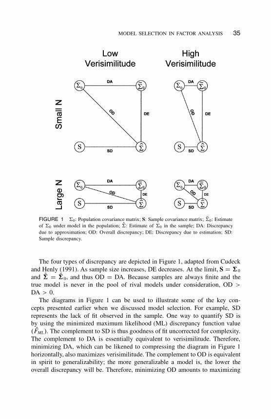
FIGURE 1 †0: Population covariance matrix; S: Sample covariance matrix; Q†0: Estimate
of †0 under model in the population; O†: Estimate of †0 in the sample; DA: Discrepancy
due to approximation; OD: Overall discrepancy; DE: Discrepancy due to estimation; SD:
Sample discrepancy.
The four types of discrepancy are depicted in Figure 1, adapted from Cudeck
and Henly (1991). As sample size increases, DE decreases. At the limit, S D †0
and O† D Q†0, and thus OD D DA. Because samples are always finite and the
true model is never in the pool of rival models under consideration, OD >
DA > 0.
The diagrams in Figure 1 can be used to illustrate some of the key con-
cepts presented earlier when we discussed model selection. For example, SD
represents the lack of fit observed in the sample. One way to quantify SD is
by using the minimized maximum likelihood (ML) discrepancy function value
. OFML/. The complement to SD is thus goodness of fit uncorrected for complexity.
The complement to DA is essentially equivalent to verisimilitude. Therefore,
minimizing DA, which can be likened to compressing the diagram in Figure 1
horizontally, also maximizes verisimilitude. The complement to OD is equivalent
in spirit to generalizability; the more generalizable a model is, the lower the
overall discrepancy will be. Therefore, minimizing OD amounts to maximizing
Dow
nloa
ded
by [
VU
L V
ande
rbilt
Uni
vers
ity]
at 1
6:24
29
Mar
ch 2
013
36 PREACHER, ZHANG, KIM, MELS
generalizability.4 DE is rarely of direct interest by itself, but it has an impact on
OD. Especially when N is small, adding parameters to a model will decrease DA
but increase DE, having opposing effects on OD (Browne & Cudeck, 1992). Ob-
taining larger samples can be likened to compressing the diagram vertically, re-
ducing DE closer to zero (Myung & Pitt, 1998), as in the lower panel of Figure 1.
Reduction of DE also makes DA and OD draw closer in magnitude. Verisimili-
tude and generalizability, therefore, are asymptotically equivalent; at very large
sample sizes, the model with the highest verisimilitude is often the model that
generalizes the best, and vice versa (Browne, 2000). In more realistic situations
with small sample sizes, some criteria select models with high verisimilitude
and others select models with high generalizability (Bandalos, 1997).
In the statistical learning literature, generalization error is defined as the
expected sample discrepancy, which is decomposed into estimation error and
approximation error. Generalization error is equivalent to OD in Cudeck and
Henly’s (1991) framework. It is known that when a model becomes more
complex, the approximation error becomes smaller but estimation error becomes
larger; this is termed the bias-variance trade-off (e.g., Heskes, 1998). The
reason the estimation error becomes larger as a model becomes more complex
may be understood in the following way: As a factor model becomes more
complex (i.e., as more factors are added), more parameters need to be estimated
using the same amount of data. Estimating more parameters while holding
the amount of data constant reduces the overall precision of estimation. Thus,
more complex models cannot be estimated as precisely as simpler models, and
this phenomenon increases as sample size decreases. To make a model more
generalizable (less variable over repeated sampling), a balance needs to be struck
between complexity and SD.
Using Cudeck and Henly’s (1991) framework, the simplest model fit indices
(e.g., root mean square residual [RMSR] and ¦2) can be best understood as
measures of SD because they are based directly on the difference between S
and O†. But minimizing SD is likely to be of less interest to the researcher than
minimizing DA or OD. Even though ¦2 is used to test the null hypothesis that
DA D 0, ¦2 and RMSR only indirectly reflect DA and OD because typically
S ¤ †0 and O† ¤ Q†0. Any fit index or selection criterion that emphasizes
cross-validation or replicability can be thought of as a measure of OD and can
4MacCallum (2003) noted that OD should be regarded as an aspect or facet of verisimilitude.
We consider OD more closely related to generalizability, which represents a model’s balance of
fit and complexity. It is possible for a model to have high verisimilitude and low generalizability
(this situation frequently occurs when models are fit to small samples, as in the top right panel of
Figure 1), but it is rare to find models with low verisimilitude and high generalizability. Because
OD � DA C DE we regard verisimilitude as an aspect of OD, not the reverse, and we consider
verisimilitude a fixed quantity that is independent of sampling.
Dow
nloa
ded
by [
VU
L V
ande
rbilt
Uni
vers
ity]
at 1
6:24
29
Mar
ch 2
013

MODEL SELECTION IN FACTOR ANALYSIS 37
be used to rank models in terms of OD or generalizability. Because OD � DA
in large samples, measures of OD and DA can be regarded as measuring the
same quantity with decreasing bias as N increases.
CRITERIA FOR SELECTING m
We now provide an overview of some methods of choosing an appropriate m.
Three different types of criteria are widely used in factor analysis literature:
criteria based on eigenvalues, criteria based on discrepancy of approximation
(reflecting verisimilitude), and criteria based on overall discrepancy (reflecting
generalizability). We do not consider eigenvalue-based criteria here as they are
less well motivated theoretically and do not fit easily within Cudeck and Henly’s
(1991) theoretical framework.
Criteria Based on Discrepancy Due to Approximation
Several criteria based on the discrepancy due to approximation (DA) are used as
measures of model fit. Two of these include the estimated population discrepancy
function .F0/ and estimated noncentrality parameter .nF0/, where n D N � 1.
However, F0 and nF0 are not applicable to model selection when generalizability
is the goal because these values decrease as a model becomes more complex.
RMSEA. The root mean square error of approximation (RMSEA; Browne
& Cudeck, 1992; Steiger & Lind, 1980) has been suggested as a factor retention
criterion. RMSEA can be regarded as an estimate of model misfit per degree of
freedom in the population. A sample point estimate of RMSEA is as follows:
RMSEA D
v
u
u
tmax
(
OFML
df�
1
n
!
; 0
)
; (3)
where OFML is the minimized ML discrepancy function value and df represents
degrees of freedom. Division by df represents an adjustment for complexity in
terms of the number of free parameters; that is, RMSEA penalizes models with
more than the necessary number of factors. RMSEA is widely regarded as a
measure of DA (Browne & Cudeck, 1992; Cudeck & Henly, 2003; MacCallum,
2003). As such, it should perform better than other criteria when the goal is to
maximize verisimilitude. In the present study, the smallest value of m for which
the RMSEA drops below .05 is selected as the most appropriate.
Dow
nloa
ded
by [
VU
L V
ande
rbilt
Uni
vers
ity]
at 1
6:24
29
Mar
ch 2
013
38 PREACHER, ZHANG, KIM, MELS
An advantage of RMSEA is that a confidence interval is easily obtained for
it, with bounds
CI D
0
@
s
OœL
df � nI
s
OœU
df � n
1
A ; (4)
where OœL and OœU are found by identifying the appropriate quantiles under
the noncentral ¦2 distribution in question (Browne & Cudeck, 1992). This
confidence interval, in turn, may be used to test hypotheses of close fit rather
than the more restrictive (and untenable) hypothesis of exact fit tested with the
likelihood ratio test. The choice of .05 as an informal criterion for close fit is
based on popular guidelines (Browne & Cudeck, 1992) and is close to the .06
value recommended by Hu and Bentler (1999) based on large-scale simulations.
We performed a separate selection procedure using the RMSEA: the smallest
value of m for which the lower bound of the RMSEA 90% confidence interval
drops below .05 was chosen as the retained number of factors. Although rigid
adherence to conventional benchmarks is not universally recommended, the use
of this procedure in the present context is consistent with choosing the smallest
m for which the test of close fit is not rejected (Browne & Cudeck, 1992;
MacCallum, Browne, & Sugawara, 1996). We term this criterion RMSEA.LB
to distinguish it from RMSEA.
Criteria Based on Overall Discrepancy
Criteria based on overall discrepancy (OD) are indices designed to select the
simplest model from a pool of rival models that most accurately describes
observed data. All information criteria include a term representing lack of fit
and a penalty term for complexity. Many information-based criteria are of the
following form:
�2fk C a � qk ; (5)
where fk is the log-likelihood associated with the model indexed by k, qk is
the number of free parameters in model k, and a is a function of sample size
(Sclove, 1987). These criteria can be used to rank models in terms of OD. If the
goal is to identify the model that maximizes generalizability, such indices may
perform well.
AIC and BIC. Two popular criteria conforming to Equation (5) are (an)
Akaike’s information criterion (AIC; Akaike, 1973) and the Bayesian informa-
tion criterion (BIC; Schwarz, 1978). For AIC, a is simply 2, whereas for BIC,
a D ln.N /. Because BIC imposes a stiffer complexity penalty than AIC for
Dow
nloa
ded
by [
VU
L V
ande
rbilt
Uni
vers
ity]
at 1
6:24
29
Mar
ch 2
013
MODEL SELECTION IN FACTOR ANALYSIS 39
N � 8, BIC generally results in the selection of models with fewer parameters
than does AIC. AIC has been shown to perform well at selecting the true number
of factors when it exists (e.g., Akaike, 1987; Bozdogan & Ramirez, 1987; Song
& Belin, 2008), but only at small N. BIC has been found to outperform AIC in
recovering the true m (e.g., Lopes & West, 2004; Song & Belin, 2008).
AIC selects more complex models as N increases because the rate of increase
in the badness of fit term increases with N, but the penalty term stays the
same (Bozdogan, 2000). This has been the basis of some questions about
the appropriateness of AIC for model selection (Ichikawa, 1988; McDonald
& Marsh, 1990; Mulaik, 2001). This tendency of AIC appears problematic
perhaps because AIC was designed with the goal of generalizability in mind
(i.e., minimizing OD), yet researchers tend to use it in pursuit of verisimilitude
(i.e., minimizing DA). Because OD � DA C DE, and DE reflects sampling
variability, it should come as no surprise that N affects model selection using
indices like AIC and BIC (Cudeck & Henly, 1991). When N is small, indices like
AIC and BIC will indicate a preference for simpler models. This phenomenon
is consistent with the earlier mentioned point that when N is small there is a
loss of precision in estimating parameters in more complex models.
A procedure closely related to ranking models by AIC or BIC is ranking
models in order of their ability to cross-validate in new data. Cross-validation
is the practice of estimating model parameters in a calibration sample and then
examining the fit of a fully constrained model in a validation sample, where all
parameters in the fully constrained model are fixed to the values estimated in
the calibration sample (i.e., Bentler’s [1980] tight replication strategy). Good fit
to the validation sample is taken as evidence of good predictive validity. Cross-
validation has received considerable support as a general strategy for selecting
the most appropriate model from a pool of alternatives in covariance structure
modeling, of which factor analysis is a special case (De Gooijer, 1995). The
reason we mention it here is that AIC can be regarded as a single-sample
estimate of an expected cross-validation criterion. The expected cross-validation
index (ECVI; Browne & Cudeck, 1992), which is equivalent to AIC when
ML estimation is used, is known to select more complex models at higher
Ns (Browne, 2000; Browne & Cudeck, 1992; Cudeck & Henly, 1991). This is
to be expected because indices based on the logic of cross-validation are not
intended to select a correct model but rather to select a model that will yield
trustworthy replication at a given N.
SUMMARY AND HYPOTHESES
To summarize, factor models (indeed, all models) are only convenient approxi-
mations constructed to aid understanding; there is no such thing as a true factor
Dow
nloa
ded
by [
VU
L V
ande
rbilt
Uni
vers
ity]
at 1
6:24
29
Mar
ch 2
013
40 PREACHER, ZHANG, KIM, MELS
model. However, out of a pool of rival explanations, one may be said to lie closest
to the data-generating process (the quasi-true model). It is reasonable to try to
identify the model with the highest relative verisimilitude because one of the
primary aims of science is to identify and understand processes that give rise to
observed data. However, even models with seemingly high verisimilitude are not
useful unless they cross-validate well in new data. Particularly in small samples,
researchers often do not have enough information to support the retention of
many factors. Therefore, we believe that identifying the model that maximizes
generalizability is a reasonable alternative (or additional) goal for researchers
to pursue. Having presented our guiding theoretical framework and having
described several FRCs, we are now in a position to make predictions about
the performance of specific FRCs in service of these dual goals.
Hypothesis 1
We have likened DA to verisimilitude. Given that verisimilitude is of great
interest to researchers, it would be useful to identify the FRC that most accurately
reflects a model’s proximity to the truth, or minimizes model error. As we have
described, the root mean square error of approximation (RMSEA) is a measure
of DA, corrected for complexity by dividing by degrees of freedom (Browne
& Cudeck, 1992; Cudeck & Henly, 1991; Steiger & Lind, 1980). Of all the
FRCs we have encountered, RMSEA and RMSEA.LB are the ones most likely
to accurately rank rival models in terms of versimilitude (DA). Other FRCs that
employ a correction for complexity approximate OD rather than DA and thus
should perform less well in finite samples when the goal is to identify the model
most similar to the data-generating process. We further note that sample size
should have little effect on DA (MacCallum, 2003) because it is a population
quantity. However, there is evidence that RMSEA is positively biased when
N < 200 and the model is well specified (see Curran, Bollen, Chen, Paxton, &
Kirby, 2003, for a good discussion of this phenomenon). This finding leads to
the expectation that RMSEA will overfactor somewhat for the smaller Ns we
investigate.
Hypothesis 2
We hypothesize that information criteria (AIC or BIC) will be good indicators
of generalizability. A guiding principle behind information criteria is that good
absolute fit to a particular data set is not by itself of central importance. Often
the analyst is interested in a model’s generalizability, or ability to predict future
data arising from the same underlying process. Theoretically, all generalizability
indices include adjustments for model complexity and can be used to rank
Dow
nloa
ded
by [
VU
L V
ande
rbilt
Uni
vers
ity]
at 1
6:24
29
Mar
ch 2
013
MODEL SELECTION IN FACTOR ANALYSIS 41
competing models in terms of OD. Many indices penalize fit for complexity, but
some employ better corrections than others. AIC and BIC should be superior
to RMSEA and RMSEA.LB in selecting the most generalizable model because
they consider all of the factors known to limit generalizability. Of the FRCs we
consider, AIC and BIC are more likely to accurately rank models in terms of
generalizability (OD) because their corrections for model complexity are well
grounded in theory. We have no prediction about which of the two (AIC or BIC)
will emerge as superior.
ILLUSTRATIVE DEMONSTRATIONS
We now present three demonstrations to illustrate that verisimilitude and gen-
eralizability are separate ideas and to determine the best criteria to use for
each goal. Fabrigar et al. (1999) expressed a need for studies such as these.
In the first demonstration, we determine what FRC is the most successful in
identifying the known data-generating model with the expectation that RMSEA
and RMSEA.LB would show superior performance (Hypothesis 1). In the second
demonstration, we determine the best FRC to use when the goal is to select
the model best able to generalize to new data arising from the same underlying
process with the expectation that information criteria would outperform RMSEA
and RMSEA.LB (Hypothesis 2). In the third demonstration we apply the various
FRCs to empirical data drawn from Jessor and Jessor’s (1991) Socialization of
Problem Behavior in Youth, 1969–1981 study.
Demonstration 1: Maximizing Verisimilitude
In order to investigate the relative abilities of FRCs to recover the quasi-true
data-generating factor model, we simulated large numbers of sample correlation
matrices from population correlation matrices that approximately satisfy a factor
analysis model. We used a procedure (Yuan & Hayashi, 2003) that produces
population correlation matrices with arbitrary RMSEAs. It can be described as
a two-stage procedure. Population correlation matrices approximately satisfying
the model are generated first; these population correlation matrices are then
transformed to correlation matrices with arbitrary RMSEAs. A property of this
two-stage procedure is that the transformation at the second stage does not
change the parameter values.
In the first stage, using Fortran, we generated population correlation matrices
using a method described by Tucker, Koopman, and Linn (1969). Manifest vari-
ables are linear combinations of three types of latent variables: major common
factors, minor common factors, and unique factors. Minor common factors are
considered in the generation of population correlation matrices so that these
Dow
nloa
ded
by [
VU
L V
ande
rbilt
Uni
vers
ity]
at 1
6:24
29
Mar
ch 2
013
42 PREACHER, ZHANG, KIM, MELS
correlation matrices approximately satisfy a factor analysis model. For each set
of three different numbers of variables (p D 9, 12, 15), population correlation
matrices with different numbers of factors were generated. The number of
factors was varied from 1 to p/3, which were 3, 4, and 5 for p D 9, 12, and
15, respectively. Major common factors contribute 60% of manifest variable
variances in all conditions. These correlation matrices involve different levels of
model error, however.
In the second stage, again using Fortran, we scaled population correlation
matrices generated in the first stage so that the population RMSEAs from
fitting the EFA model to the scaled population correlation matrices are all
.05. Population correlation matrices generated in the first stage were partitioned
into two parts: the model implied correlation matrix and the residual matrix.
A population correlation matrix with an arbitrary RMSEA can be obtained
by adding a properly scaled residual matrix to the model implied correlation
matrix. This two-stage procedure was repeated 1,000 times within each cell of
the design, yielding 12,000 population matrices.
Sample correlation matrices were generated from these population matrices
using a method described by Wijsman (1959) and implemented in Fortran.
Sample size was manipulated to correspond to a range of values typically seen
in applied research (N D 100, 500, 1,000, 3,000). All factor models were fit
to generated matrices using ML as implemented in the factor analysis software
CEFA 3.04 (Browne, Cudeck, Tateneni, & Mels, 2008). By applying four FRCs
(RMSEA, RMSEA.LB, AIC, and BIC), the optimal number of factors was
selected for each correlation matrix. Because selection of the quasi-true data-
generating model was the only criterion for success in this demonstration, factor
solutions were not rotated. Of primary interest was whether or not RMSEA and
RMSEA.LB would prove to be better FRCs than information-based indices.
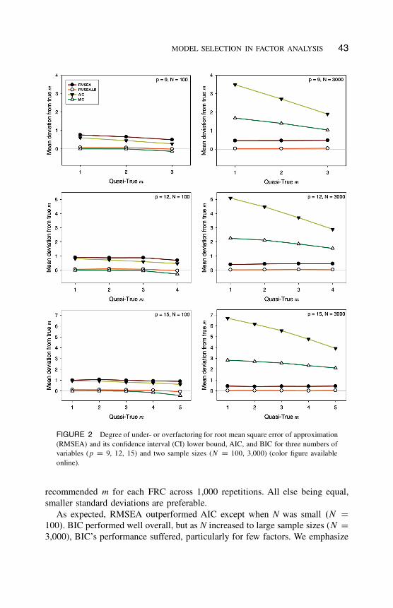
Figure 2 shows the difference between the mean number of selected factors
and the quasi-true number of factors. We chose to plot results only for N D 100
and 3,000 (results for N D 500 and 1,000 are provided online at the first author’s
website5). In the plots, positive numbers represent overfactoring with respect
to the quasi-true m and negative numbers represent underfactoring. Overall,
overfactoring was a more regular occurrence than underfactoring. As expected,
RMSEA had a tendency to overfactor in small samples .N D 100/. The RMSEA
lower bound rarely overfactored, and its good performance was not affected by
sample size. AIC performed well in small samples .N D 100/ but had a tendency
to severely overfactor in larger samples (i.e., N D 500 in our simulation),
especially for small numbers of factors. BIC also overfactored as N increased
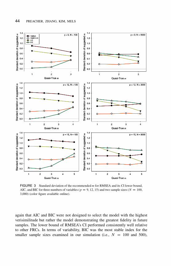
but not as severely as AIC. Figure 3 displays the standard deviation of the
5http://quantpsy.org
Dow
nloa
ded
by [
VU
L V
ande
rbilt
Uni
vers
ity]
at 1
6:24
29
Mar
ch 2
013
MODEL SELECTION IN FACTOR ANALYSIS 43
FIGURE 2 Degree of under- or overfactoring for root mean square error of approximation
(RMSEA) and its confidence interval (CI) lower bound, AIC, and BIC for three numbers of
variables (p D 9, 12, 15) and two sample sizes (N D 100, 3,000) (color figure available
online).
recommended m for each FRC across 1,000 repetitions. All else being equal,
smaller standard deviations are preferable.
As expected, RMSEA outperformed AIC except when N was small .N D100/. BIC performed well overall, but as N increased to large sample sizes (N D
3,000), BIC’s performance suffered, particularly for few factors. We emphasize
Dow
nloa
ded
by [
VU
L V
ande
rbilt
Uni
vers
ity]
at 1
6:24
29
Mar
ch 2
013
44 PREACHER, ZHANG, KIM, MELS
FIGURE 3 Standard deviation of the recommended m for RMSEA and its CI lower bound,
AIC, and BIC for three numbers of variables (p D 9, 12, 15) and two sample sizes (N D 100,
3,000) (color figure available online).
again that AIC and BIC were not designed to select the model with the highest
verisimilitude but rather the model demonstrating the greatest fidelity in future
samples. The lower bound of RMSEA’s CI performed consistently well relative
to other FRCs. In terms of variability, BIC was the most stable index for the
smaller sample sizes examined in our simulation (i.e., N D 100 and 500),
Dow
nloa
ded
by [
VU
L V
ande
rbilt
Uni
vers
ity]
at 1
6:24
29
Mar
ch 2
013
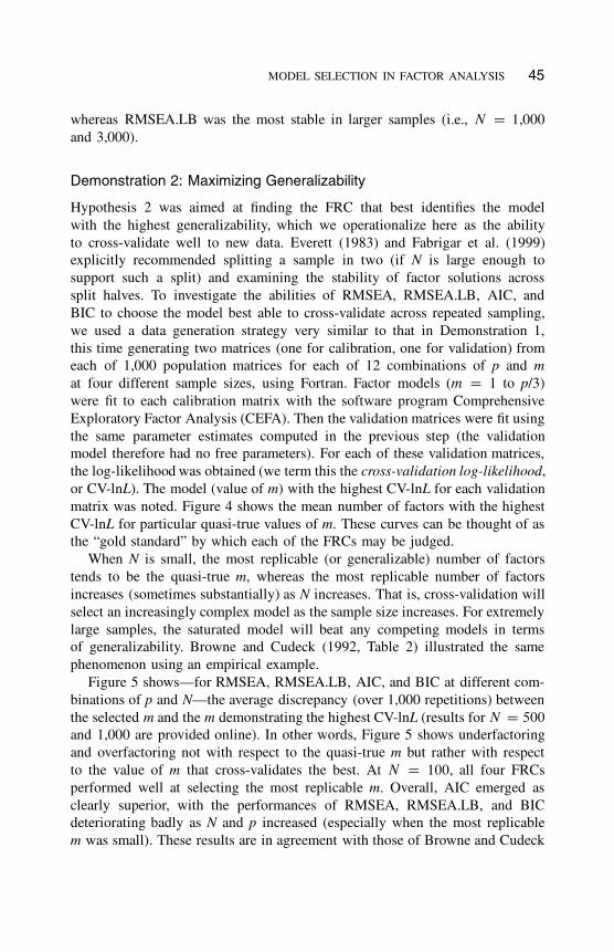
MODEL SELECTION IN FACTOR ANALYSIS 45
whereas RMSEA.LB was the most stable in larger samples (i.e., N D 1,000
and 3,000).
Demonstration 2: Maximizing Generalizability
Hypothesis 2 was aimed at finding the FRC that best identifies the model
with the highest generalizability, which we operationalize here as the ability
to cross-validate well to new data. Everett (1983) and Fabrigar et al. (1999)
explicitly recommended splitting a sample in two (if N is large enough to
support such a split) and examining the stability of factor solutions across
split halves. To investigate the abilities of RMSEA, RMSEA.LB, AIC, and
BIC to choose the model best able to cross-validate across repeated sampling,
we used a data generation strategy very similar to that in Demonstration 1,
this time generating two matrices (one for calibration, one for validation) from
each of 1,000 population matrices for each of 12 combinations of p and m
at four different sample sizes, using Fortran. Factor models (m D 1 to p/3)
were fit to each calibration matrix with the software program Comprehensive
Exploratory Factor Analysis (CEFA). Then the validation matrices were fit using
the same parameter estimates computed in the previous step (the validation
model therefore had no free parameters). For each of these validation matrices,
the log-likelihood was obtained (we term this the cross-validation log-likelihood,
or CV-lnL). The model (value of m) with the highest CV-lnL for each validation
matrix was noted. Figure 4 shows the mean number of factors with the highest
CV-lnL for particular quasi-true values of m. These curves can be thought of as
the “gold standard” by which each of the FRCs may be judged.
When N is small, the most replicable (or generalizable) number of factors
tends to be the quasi-true m, whereas the most replicable number of factors
increases (sometimes substantially) as N increases. That is, cross-validation will
select an increasingly complex model as the sample size increases. For extremely
large samples, the saturated model will beat any competing models in terms
of generalizability. Browne and Cudeck (1992, Table 2) illustrated the same
phenomenon using an empirical example.
Figure 5 shows—for RMSEA, RMSEA.LB, AIC, and BIC at different com-
binations of p and N—the average discrepancy (over 1,000 repetitions) between
the selected m and the m demonstrating the highest CV-lnL (results for N D 500
and 1,000 are provided online). In other words, Figure 5 shows underfactoring
and overfactoring not with respect to the quasi-true m but rather with respect
to the value of m that cross-validates the best. At N D 100, all four FRCs
performed well at selecting the most replicable m. Overall, AIC emerged as
clearly superior, with the performances of RMSEA, RMSEA.LB, and BIC
deteriorating badly as N and p increased (especially when the most replicable
m was small). These results are in agreement with those of Browne and Cudeck
Dow
nloa
ded
by [
VU
L V
ande
rbilt
Uni
vers
ity]
at 1
6:24
29
Mar
ch 2
013
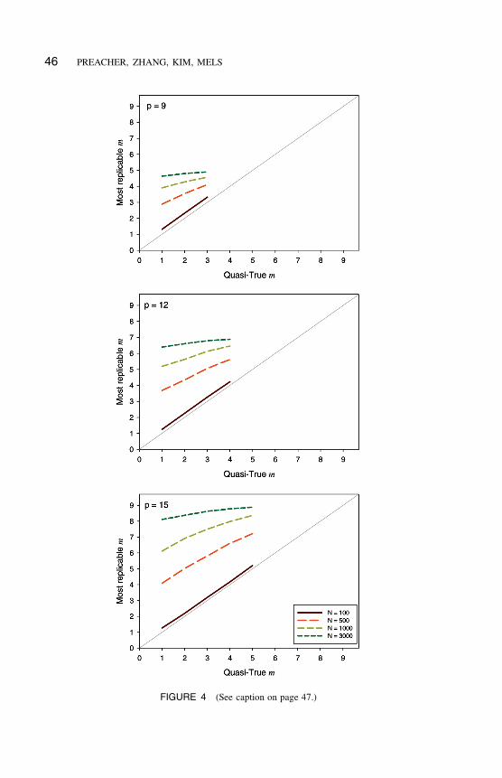
46 PREACHER, ZHANG, KIM, MELS
FIGURE 4 (See caption on page 47.)
Dow
nloa
ded
by [
VU
L V
ande
rbilt
Uni
vers
ity]
at 1
6:24
29
Mar
ch 2
013

MODEL SELECTION IN FACTOR ANALYSIS 47
(1989). BIC, the other information-based criterion we examined, outperformed
RMSEA and RMSEA.LB but still underfactored.
Demonstration 3: Jessor and Jessor’s (1991) Values Data
We now illustrate how different goals, and use of FRCs consistent with each
of those goals, can lead to different model selection decisions in practice. We
make use of Jessor and Jessor’s (1991) Socialization of Problem Behavior in
Youth, 1969–1981 study. Specifically, we use the 30 items of the Personal Values
Questionnaire (PVQ; Jessor & Jessor, 1977), originally administered to 432
Colorado high school students in 1969–1972, but we make use of only the
1969 data. The PVQ was intended to tap three underlying dimensions: values
on academic achievement (VAC), values on social love (VSL), and values on
independence (VIN). There are no reverse-scored items, all items were scored
on a 10-point Likert scale (0 D Neither like nor dislike; 9 D Like very much),
and items from the three subscales were presented in a mixed order. Example
items were (for VAC) “How strongly do I like to have good grades to go on
to college if I want to?,” (for VSL) “How strongly to I like to get along well
with other kids?,” and (for VIN) “How strongly do I like to be able to decide
for myself how to spend my free time?”
Researchers using the PVQ may reasonably hope for good fit for the three-
factor model in a given sample with the hope that this good fit implies good fit
in the population (i.e., high verisimilitude) but may also hope that this model
stands a reasonable chance of cross-validating to other samples from the same
population (i.e., high generalizability). We randomly selected 212 students from
the 425 students with complete data on all 30 items and fit factor models with
m ranging from 2 to 10. We employed EFA with ML estimation in Mplus 6.12
(Muthén & Muthén, 1998–2011). Oblique quartimax (direct quartimin) rotation
was used in all models. All of the investigated FRCs are reported in Table 1. It
is clear from the results in Table 1 that RMSEA.LB favors a three-factor model,
in line with the original authors’ expectations. Few of the loadings are large,
but most follow the expected pattern. Overall, it is reasonable to conclude that
m D 3 is the quasi-true number of factors for these data, in line with the authors’
intent. However, a fourth factor could be retained that borrows items from the
other three factors and which is subject to a separate substantive interpretation.
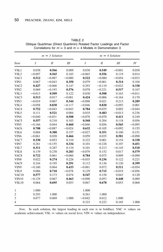
We report loadings and factor correlations from the m D 3 and m D 4 analyses
in Table 2.
FIGURE 4 (See artwork on page 46.) The abscissa lists the quasi-true number of factors
(m); the ordinate represents the mean number of factors with the highest cross-validation
log-likelihood (CV-lnL) for particular values of m (color figure available online).
Dow
nloa
ded
by [
VU
L V
ande
rbilt
Uni
vers
ity]
at 1
6:24
29
Mar
ch 2
013
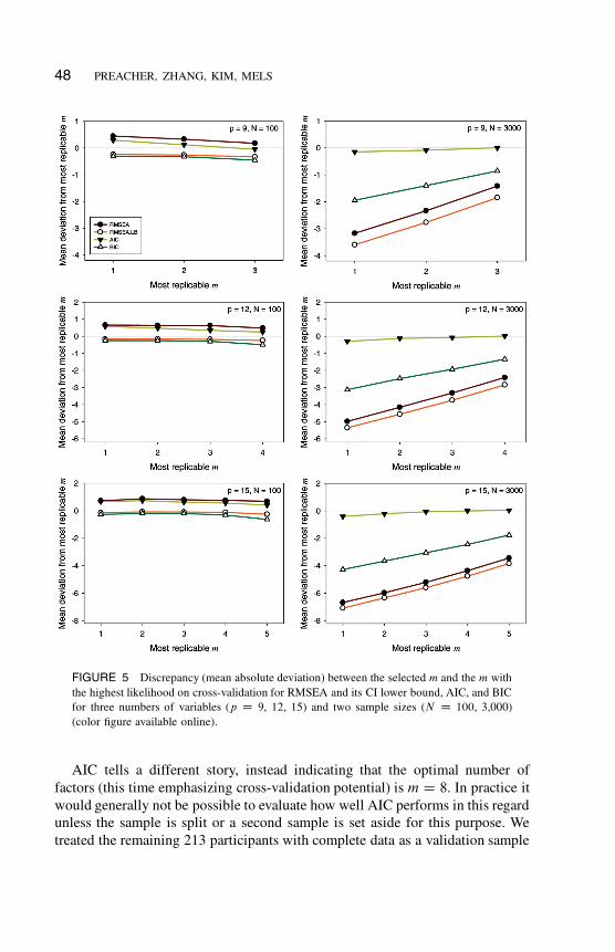
48 PREACHER, ZHANG, KIM, MELS
FIGURE 5 Discrepancy (mean absolute deviation) between the selected m and the m with
the highest likelihood on cross-validation for RMSEA and its CI lower bound, AIC, and BIC
for three numbers of variables (p D 9, 12, 15) and two sample sizes (N D 100, 3,000)
(color figure available online).
AIC tells a different story, instead indicating that the optimal number of
factors (this time emphasizing cross-validation potential) is m D 8. In practice it
would generally not be possible to evaluate how well AIC performs in this regard
unless the sample is split or a second sample is set aside for this purpose. We
treated the remaining 213 participants with complete data as a validation sample
Dow
nloa
ded
by [
VU
L V
ande
rbilt
Uni
vers
ity]
at 1
6:24
29
Mar
ch 2
013

MODEL SELECTION IN FACTOR ANALYSIS 49
TABLE 1
Factor Retention Criteria and Cross-Validation Log-Likelihood for
Factor Models in Demonstration 3
Calibration Validation
m AIC BIC RMSEA RMSEA.LB CV-lnL
2 17,055.489 17,354.225 .078 .071 �8,381.557
3 16,852.055 17,244.776* .059 .051 �8,219.392
4 16,810.006 17,293.355 .052 .044* �8,208.548
5 16,786.896 17,357.516 .047* .037 �8,209.348
6 16,772.804 17,427.338 .041 .030 �8,202.758
7 16,773.172 17,508.265 .038 .025 �8,198.476*
8 16,766.226* 17,578.520 .031 .013 �8,210.157
9 16,769.116 17,655.255 .025 .000 �8,238.995
10a 16,779.801 17,736.428 .020 .000 �8,236.739
Note. m D number of factors; AIC D Akaike’s (an) information criterion; BIC D Bayesian
information criterion; RMSEA D root mean square error of approximation; RMSEA.LB D RMSEA
90% confidence interval lower bound; CV-lnL D cross-validation log-likelihood.aThe 10-factor solution contained an extremely large negative unique variance for the fourth
values on social love (VSL) item, compromising the admissibility and interpretability of this solution.
*Asterisks indicate the selected model (for AIC, BIC, RMSEA, and RMSEA.LB) or the model
with the highest CV-lnL.
for the factor structures we earlier estimated using the calibration sample. We
fit each of our models to the validation sample, fully constraining each model
to parameter values estimated using the calibration sample. Agreeing closely
with expectations based on AIC, the model with the highest cross-validation
log-likelihood is the m D 7 model, with the highest (least negative) CV-lnL
out of all nine competing models (see the final column of Table 1). Thus,
AIC selected a model very nearly the most generalizable, as reflected in the
fit of the fully parameterized model to an independent sample. After a point
the loadings become difficult to interpret, but the most interpretable number of
factors lies somewhere between m D 3 and m D 8. Complete results from this
demonstration are available online.
Demonstration Summary
The implications of these demonstrations for the applied researcher are clear. If
the researcher were curious about the number and nature of factors underlying
the data in hand, RMSEA and (especially) RMSEA.LB are good choices. BIC’s
choice was unexpectedly in agreement with RMSEA and RMSEA.LB for most
of the Ns examined. Demonstrations 1 and 2 suggest that BIC is not particularly
Dow
nloa
ded
by [
VU
L V
ande
rbilt
Uni
vers
ity]
at 1
6:24
29
Mar
ch 2
013
50 PREACHER, ZHANG, KIM, MELS
TABLE 2
Oblique Quartimax (Direct Quartimin) Rotated Factor Loadings and Factor
Correlations for m D 3 and m D 4 Models in Demonstration 3
m D 3 Solution m D 4 Solution
Item I II III I II III IV
VSL1 0.038 0.566 0.009 0.038 0.549 �0.001 0.058
VSL2 �0.097 0.565 0.103 �0.065 0.556 0.119 0.014
VAC1 0.512 �0.087 �0.080 0.522 �0.080 �0.054 �0.033
VIN1 0.067 �0.043 0.350 0.079 �0.061 0.314 0.104
VAC2 0.427 �0.068 0.147 0.293 �0.119 �0.022 0.338
VIN2 0.069 �0.193 0.576 0.078 �0.221 0.517 0.167
VSL3 �0.013 0.509 0.122 0.030 0.508 0.163 �0.011
VAC3 0.513 0.017 �0.081 0.424 �0.006 �0.164 0.170
VIN3 �0.019 0.067 0.344 �0.098 0.021 0.213 0.289
VSL4 �0.058 0.830 �0.117 �0.046 0.820 �0.093 0.001
VAC4 0.752 �0.043 �0.043 0.784 �0.035 0.003 �0.044
VSL5 0.111 0.521 0.084 0.035 0.483 �0.013 0.236
VIN4 �0.040 �0.031 0.508 �0.078 �0.070 0.411 0.249
VAC5 0.557 0.210 0.103 0.568 0.204 0.118 0.056
VIN5 �0.166 0.044 0.460 �0.046 0.056 0.565 �0.095
VAC6 0.708 �0.087 �0.024 0.632 �0.105 �0.092 0.155
VSL6 0.004 0.380 0.157 �0.027 0.351 0.100 0.151
VIN6 �0.061 0.020 0.466 0.059 0.035 0.581 �0.098
VAC7 0.330 0.053 0.310 0.222 0.001 0.154 0.338
VIN7 0.261 �0.155 0.334 0.101 �0.228 0.107 0.451
VSL7 0.311 0.287 0.110 0.101 0.213 �0.145 0.518
VSL8 0.139 0.238 0.283 �0.079 0.152 0.017 0.579
VAC8 0.722 0.061 �0.060 0.784 0.075 0.009 �0.090
VIN8 0.022 0.274 0.226 �0.035 0.236 0.122 0.221
VAC9 0.244 0.195 0.291 0.112 0.136 0.120 0.399
VIN9 �0.160 0.064 0.433 �0.061 0.072 0.511 �0.054
VSL9 0.086 0.710 �0.078 0.129 0.715 �0.019 �0.056
VAC10 0.577 0.173 0.074 0.547 0.158 0.043 0.120
VIN10 �0.129 0.067 0.463 �0.098 0.053 0.448 0.089
VSL10 0.064 0.695 0.053 0.067 0.678 0.053 0.068
1 1.000 1.000
2 0.293 1.000 0.261 1.000
3 0.077 0.069 1.000 �0.042 0.012 1.000
4 0.323 0.223 0.165 1.000
Note. In each solution, the largest loading in each row is in boldface. VAC D values on
academic achievement; VSL D values on social love; VIN D values on independence.
Dow
nloa
ded
by [
VU
L V
ande
rbilt
Uni
vers
ity]
at 1
6:24
29
Mar
ch 2
013
MODEL SELECTION IN FACTOR ANALYSIS 51
useful for identifying the most replicable m, except perhaps at very large N.
Instead, AIC performed well at selecting a generalizable model with strong
cross-validation potential.
DISCUSSION
Cudeck and Henly (1991) state, “It may be better to use a simple model in
a small sample rather than one that perhaps is more realistically complex but
that cannot be accurately estimated” (p. 513), a point echoed by Browne and
Cudeck (1992). We agree. Our treatment owes much to these sources. In this
article we apply these ideas to the context of choosing the number of factors in
exploratory factor analysis, emphasizing and illustrating a distinction between
the behavior of indices that minimize OD (i.e., those that select m on the basis
of generalizability) and those that minimize DA (i.e., those that select m on the
basis of verisimilitude). Proceeding from the reasonable assumption that cross-
validation and replication are both worthy scientific goals, we emphasize that it is
often worthwhile to seek the value of m that yields the most generalizable factor
model in a given setting. This is the model, out of all competing alternatives, that
shows the best balance of goodness of fit and parsimony and the one that best
predicts future data (i.e., minimizes OD). We recommend using AIC as a factor
retention criterion if generalizability is the goal. At the same time, we recognize
that another worthwhile goal of science is to search for the objective truth.
Often researchers would like to find the one model out of several competing
models that best approximates the objectively true data-generating process (i.e.,
the model that minimizes DA), even if that model is not likely to generalize well
in future samples. For this goal, we recommend using RMSEA.LB. RMSEA.LB
performed well at recovering the quasi-true number of factors at all investigated
sample sizes. Both goals can be explicitly pursued in the same study to yield a
more thorough, well-considered analysis.
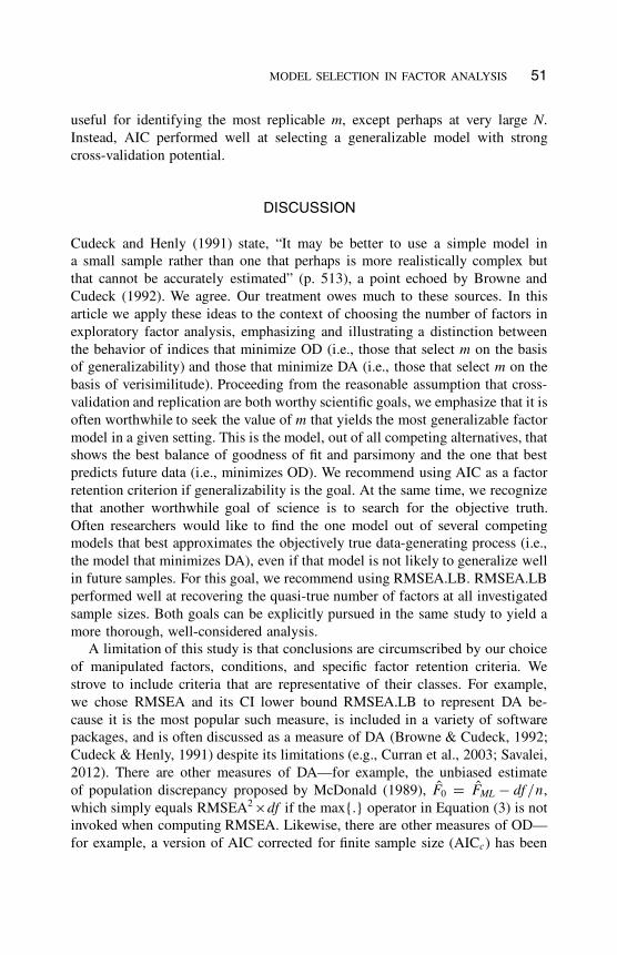
A limitation of this study is that conclusions are circumscribed by our choice
of manipulated factors, conditions, and specific factor retention criteria. We
strove to include criteria that are representative of their classes. For example,
we chose RMSEA and its CI lower bound RMSEA.LB to represent DA be-
cause it is the most popular such measure, is included in a variety of software
packages, and is often discussed as a measure of DA (Browne & Cudeck, 1992;
Cudeck & Henly, 1991) despite its limitations (e.g., Curran et al., 2003; Savalei,
2012). There are other measures of DA—for example, the unbiased estimate
of population discrepancy proposed by McDonald (1989), OF0 D OFML � df =n,
which simply equals RMSEA2 �df if the max{.} operator in Equation (3) is not
invoked when computing RMSEA. Likewise, there are other measures of OD—
for example, a version of AIC corrected for finite sample size (AICc) has been
Dow
nloa
ded
by [
VU
L V
ande
rbilt
Uni
vers
ity]
at 1
6:24
29
Mar
ch 2
013
52 PREACHER, ZHANG, KIM, MELS
recommended for use when N is small relative to qk (Burnham & Anderson,
2004). It is possible that conclusions would differ had other measures of OD or
DA been included, so caution should be exercised in extending our conclusions
to criteria other than those we investigated.
It is our experience that indices developed with generalizability in mind are
commonly misapplied for the purpose of selecting the model with the most
verisimilitude. For example, AIC has been criticized because it has a tendency
to favor more complex models as N increases, even though the choice of
what model is the most objectively correct should not depend on sample size
(McDonald, 1989; McDonald & Marsh, 1990; Mulaik, 2001). But selecting a
model based on its objective correctness does not guarantee that it will be useful
in predicting future data, and vice versa, so we agree with Browne (2000) and
Cudeck and Henly (1991) that this criticism is not entirely justified. Even if the
“true” model is known with certainty, in small samples parameter estimates are
so unstable from sample to sample that accurate prediction of future samples
often cannot be achieved.
To summarize, researchers should consider adopting a model selection strat-
egy when choosing m. We join Grünwald (2000) in emphasizing that model
selection is not intended to find the true model but rather is intended to identify
a parsimonious model that gives reasonable fit. In the context of factor analysis,
this strategy involves identifying a few theoretically plausible values for m
before data are collected. It also involves recognizing that generalizability (a
model’s potential to cross-validate) and verisimilitude (a model’s proximity
to the objective truth) are not synonymous and therefore constitute separate
goals in model fitting and theory testing. Because both goals are generally
worth pursuing, we advocate using generalizability as a criterion for success
in addition to closeness to the truth. There is little utility in identifying the
approximately correct m if the factors fail to replicate over repeated sampling
(McCrae, Zonderman, Costa, Bond, & Paunonen, 1996). When selection with
respect to verisimilitude and generalizability lead to choosing different models,
we suggest selecting the more generalizable model as long as its absolute fit is
judged to lie within acceptable limits and the factors remain interpretable. These
points apply more broadly than the factor analysis context; in fact, the indices
we used as FRCs in this study are commonly used as model selection criteria
in more general latent variable analyses like structural equation modeling (of
which EFA is a special case). Choosing models with high verisimilitude and
generalizability is also of interest in those contexts. However, because these
criteria may perform differently in contexts other than EFA, our simulation
results should not be generalized beyond EFA without further investigation.
Choosing m is a difficult problem to which there is no clear solution. Follow-
ing the recommendations of many psychometricians (e.g., Nunnally & Bernstein,
1994), perhaps the best strategy is to use several criteria in conjunction to con-
Dow
nloa
ded
by [
VU
L V
ande
rbilt
Uni
vers
ity]
at 1
6:24
29
Mar
ch 2
013
MODEL SELECTION IN FACTOR ANALYSIS 53
verge on the most appropriate value for m. We again emphasize that regardless of
the decision aids employed, the retained factors must be interpretable in light of
theory. Factor analysis involves identifying an appropriate number of factors,
choosing an estimation method, conducting factor rotation, and interpreting
rotated factor loadings and factor correlations. Decisions made in any step have
a profound influence on other steps and thus affect the overall quality of factor
analysis results. We believe the strategy of employing different factor retention
criteria for different purposes will improve applications of factor analysis.
ACKNOWLEDGMENTS
This study made use of the Socialization of Problem Behavior in Youth, 1969–
1981 data made available by Richard and Shirley Jessor in 1991. The data are
available through the Henry A. Murray Research Archive at Harvard University
(producer and distributor). We are indebted to Daniel J. Navarro and anonymous
reviewers for valuable input.
REFERENCES
Akaike, H. (1973). Information theory and an extension of the maximum likelihood principle. In
B. N. Petrov & F. Csaki (Eds.), Second international symposium on information theory (pp.
267–281). Budapest, Hungary: Akademia Kiado.
Akaike, H. (1987). Factor analysis and AIC. Psychometrika, 52, 317–332.
Bandalos, D. L. (1997). Assessing sources of error in structural equation models: The effects of
sample size, reliability, and model misspecification. Structural Equation Modeling, 4, 177–192.
Bentler, P. M. (1980). Multivariate analysis with latent variables: Causal modeling. Annual Review
of Psychology, 31, 419–456.
Bentler, P. M., & Mooijaart, A. (1989). Choice of structural model via parsimony: A rationale based
on precision. Psychological Bulletin, 106, 315–317.
Bollen, K. A. (1989). Structural equations with latent variables. New York, NY: Wiley.
Box, G. E. P. (1976). Science and statistics. Journal of the American Statistical Association, 71,
791–799.
Bozdogan, H. (2000). Akaike’s information criterion and recent developments in information com-
plexity. Journal of Mathematical Psychology, 44, 62–91.
Bozdogan, H., & Ramirez, D. E. (1987). An expert model selection approach to determine the “best”
pattern structure in factor analysis models. In H. Bozdogan & A. K. Gupta (Eds.), Multivariate
statistical modeling and data analysis (pp. 35–60). Dordrecht, The Netherlands: D. Reidel.
Browne, M. W. (2000). Cross-validation methods. Journal of Mathematical Psychology, 44, 108–
132.
Browne, M. W. (2001). An overview of analytic rotation in exploratory factor analysis. Multivariate
Behavioral Research, 36, 111–150.
Browne, M. W., & Cudeck, R. (1989). Single sample cross-validation indices for covariance struc-
tures. Multivariate Behavioral Research, 24, 445–455.
Browne, M. W., & Cudeck, R. (1992). Alternative ways of assessing model fit. Sociological Methods
and Research, 21, 230–258.
Dow
nloa
ded
by [
VU
L V
ande
rbilt
Uni
vers
ity]
at 1
6:24
29
Mar
ch 2
013
54 PREACHER, ZHANG, KIM, MELS
Browne, M. W., Cudeck, R., Tateneni, K., & Mels, G. (2008). CEFA: Comprehensive exploratory
factor analysis. Retrieved from http://faculty.psy.ohio-state.edu/browne/
Burnham, K. P., & Anderson, D. R. (2004). Multimodel inference: Understanding AIC and BIC in
model selection. Sociological Methods & Research, 33, 261–304.
Cattell, R. B. (1966). The scree test for the number of factors. Multivariate Behavioral Research,
1, 245–276.
Collyer, C. E. (1985). Comparing strong and weak models by fitting them to computer-generated
data. Perception and Psychophysics, 38, 476–481.
Comrey, A. L., & Lee, H. B. (1992). A first course in factor analysis (2nd ed.). Hillsdale, NJ:
Erlbaum.
Costa, P. T., Jr., & McCrae, R. R. (1992). Normal personality assessment in clinical practice: The
NEO Personality Inventory. Psychological Assessment, 4, 5–13.
Cudeck, R. (1991). Comments on “Using causal models to estimate indirect effects.” In L. M.
Collins & J. L. Horn (Eds.), Best methods for the analysis of change: Recent advances, unanswered
questions, future directions (pp. 260–263). Washington, DC: American Psychological Association.
Cudeck, R., & Henly, S. J. (1991). Model selection in covariance structures analysis and the
“problem” of sample size: A clarification. Psychological Bulletin, 109, 512–519.
Cudeck, R., & Henly, S. J. (2003). A realistic perspective on pattern representation in growth data:
Comment on Bauer and Curran (2003). Psychological Methods, 8, 378–383.
Curran, P. J., Bollen, K. A., Chen, F., Paxton, P., & Kirby, J. B. (2003). Finite sampling properties
of the point estimates and confidence intervals of the RMSEA. Sociological Methods & Research,
32, 208–252.
Cutting, J. E. (2000). Accuracy, scope, and flexibility of models. Journal of Mathematical Psychol-
ogy, 44, 3–19.
Cutting, J. E., Bruno, N., Brady, N. P., & Moore, C. (1992). Selectivity, scope, and simplicity of
models: A lesson from fitting judgments of perceived depth. Journal of Experimental Psychology:
General, 121, 364–381.
De Gooijer, J. G. (1995). Cross-validation criteria for covariance structures. Communications in
Statistics: Simulation and Computation, 24, 1–16.
Dunn, J. C. (2000). Model complexity: The fit to random data reconsidered. Psychological Research,
63, 174–182.
Everett, J. E. (1983). Factor comparability as a means of determining the number of factors and
their rotation. Multivariate Behavioral Research, 18, 197–218.
Eysenck, H. J. (1991). Dimensions of personality: 16, 5, or 3? Criteria for a taxonomic paradigm.
Personality and Individual Differences, 12, 773–790.
Fabrigar, L. R., Wegener, D. T., MacCallum, R. C., & Strahan, E. J. (1999). Evaluating the use of
exploratory factor analysis in psychological research. Psychological Methods, 4, 272–299.
Grünwald, P. D. (2000). Model selection based on minimum description length. Journal of Mathe-
matical Psychology, 44, 133–152.
Heskes, T. (1998). Bias/variance decomposition for likelihood-based estimators. Neural Computa-
tion, 10, 1425–1433.
Hu, L., & Bentler, P. M. (1999). Cutoff criteria in fix indexes in covariance structure analysis:
Conventional criteria versus new alternatives. Structural Equation Modeling, 6, 1–55.
Hubbard, R., & Allen, S. J. (1989). On the number and nature of common factors extracted by the
eigenvalue-one rule using BMDP vs. SPSSx. Psychological Reports, 65, 155–160.
Humphreys, L. G. (1964). Number of cases and number of factors: An example where N is very
large. Educational and Psychological Measurement, 24, 457–466.
Ichikawa, M. (1988). Empirical assessments of AIC procedure for model selection in factor analysis.
Behaviormetrika, 24, 33–40.
Jessor, R., & Jessor, S. L. (1977). Problem behavior and psychosocial development: A longitudinal
study of youth. New York, NY: Academic Press.
Dow
nloa
ded
by [
VU
L V
ande
rbilt
Uni
vers
ity]
at 1
6:24
29
Mar
ch 2
013
MODEL SELECTION IN FACTOR ANALYSIS 55
Jessor, R., & Jessor, S. L. (1991). Socialization of problem behavior in youth, 1969–1981 [http://hdl.
handle.net/1902.1/00782, UNF:3:bNvdfUO8c9YXemVwScJy/A==]. Henry A. Murray Research
Archive (http://www.murray.harvard.edu/), Cambridge, MA.
Leahy, K. (1994). The overfitting problem in perspective. AI Expert, 9, 35–36.
Linhart, H., & Zucchini, W. (1986). Model selection. New York, NY: Wiley.
Lopes, H. F., & West, M. (2004). Bayesian model assessment in factor analysis. Statistica Sinica,
14, 41–67.
MacCallum, R. C. (2003). Working with imperfect models. Multivariate Behavioral Research, 38,
113–139.
MacCallum, R. C., Browne, M. W., & Cai, L. (2007). Factor analysis models as approximations:
Some history and some implications. In R. Cudeck & R. C. MacCallum (Eds.), Factor analysis
at 100: Historical developments and future directions (pp. 153–175). Mahwah, NJ: Erlbaum.
MacCallum, R. C., Browne, M. W., & Sugawara, H. M. (1996). Power analysis and determination
of sample size for covariance structure modeling. Psychological Methods, 1, 130–149.
MacCallum, R. C., & Tucker, L. R. (1991). Representing sources of error in the common factor
model: Implications for theory and practice. Psychological Bulletin, 109, 502–511.
McCrae, R. R., Zonderman, A. B., Costa, P. T., Jr., Bond, M. H., & Paunonen, S. V. (1996).
Evaluating replicability of factors in the revised NEO Personality Inventory: Confirmatory factor
analysis versus Procrustes rotation. Journal of Personality and Social Psychology, 70, 552–566.
McDonald, R. P. (1989). An index of goodness-of-fit based on noncentrality. Journal of Classifica-
tion, 6, 97–103.
McDonald, R. P., & Marsh, H. W. (1990). Choosing a multivariate model: Noncentrality and
goodness of fit. Psychological Bulletin, 107, 247–255.
Meehl, P. E. (1990). Appraising and amending theories: The strategy of Lakatosian defense and two
principles that warrant it. Psychological Inquiry, 1, 108–141.
Mulaik, S. A. (2001). The curve-fitting problem: An objectivist view. Philosophy of Science, 68,
218–241.
Mulaik, S. A., James, L. R., Van Alstine, J., Bennett, N., Lind, S., & Stilwell, C. D. (1989).
Evaluation of goodness-of-fit indices for structural equation models. Psychological Bulletin, 105,
430–445.
Muthén, L. K., & Muthén, B. O. (1998–2011). Mplus user’s guide (6th ed.). Los Angeles, CA:
Author.
Myung, I. J. (2000). The importance of complexity in model selection. Journal of Mathematical
Psychology, 44, 190–204.
Myung, I. J., & Pitt, M. A. (1998). Issues in selecting mathematical models of cognition. In J.
Grainger & A. M. Jacobs (Eds.), Localist connectionist approaches to human cognition (pp.
327–355). Mahwah, NJ: Erlbaum.
Nunnally, J. C., & Bernstein, I. H. (1994). Psychometric theory (3rd ed.). New York, NY: McGraw-
Hill.
Pitt, M. A., & Myung, I. J. (2002). When a good fit can be bad. Trends in Cognitive Sciences, 6,
421–425.
Pitt, M. A., Myung, I. J., & Zhang, S. (2002). Toward a method of selecting among computational
models of cognition. Psychological Review, 109, 472–491.
Platt, J. R. (1964, October 16). Strong inference. Science, 146(3642), 347–353.
Popper, K. R. (1959). The logic of scientific discovery. London, UK: Hutchinson.
Preacher, K. J. (2006). Quantifying parsimony in structural equation modeling. Multivariate Behav-
ioral Research, 41, 227–259.
Roberts, S., & Pashler, H. (2000). How persuasive is a good fit? A comment on theory testing.
Psychological Review, 107, 358–367.
Savalei, V. (2012). The relationship between RMSEA and model misspecification in CFA models.
Educational and Psychological Measurement, 72, 910–932.
Dow
nloa
ded
by [
VU
L V
ande
rbilt
Uni
vers
ity]
at 1
6:24
29
Mar
ch 2
013

56 PREACHER, ZHANG, KIM, MELS
Schwarz, G. (1978). Estimating the dimension of a model. Annals of Statistics, 6, 461–464.
Sclove, S. L. (1987). Application of model-selection criteria to some problems in multivariate
analysis. Psychometrika, 52, 333–343.
Song, J., & Belin, T. R. (2008). Choosing an appropriate number of factors in factor analysis with
incomplete data. Computational Statistics and Data Analysis, 52, 3560–3569.
Steiger, J. H., & Lind, J. C. (1980, May). Statistically based tests for the number of common factors.
Paper presented at the annual meeting of the Psychometric Society, Iowa City, IA.
Thompson, B. (1994). The pivotal role of replication in psychological research: Empirically evalu-
ating the replicability of sample results. Journal of Personality, 62, 157–176.
Thurstone, L. L. (1947). Multiple-factor analysis: A development and expansion of The Vectors of
the Mind. Chicago, IL: The University of Chicago Press.
Tucker, L. R., Koopman, R. F., & Linn, R. L. (1969). Evaluation of factor analytic research
procedures by means of simulated correlation matrices. Psychometrika, 34, 421–459.
Wijsman, R. A. (1959). Applications of a certain representation of the Wishart matrix. Annals of
Mathematical Statistics, 30, 597–601.
Yuan, K., & Hayashi, K. (2003). Bootstrap approach to inference and power analysis based on three
test statistics for covariance structure models. British Journal of Mathematical and Statistical
Psychology, 56, 93–110.
Zwick, W. R., & Velicer, W. F. (1986). Comparison of five rules for determining the number of
components to retain. Psychological Bulletin, 99, 432–442.
Dow
nloa
ded
by [
VU
L V
ande
rbilt
Uni
vers
ity]
at 1
6:24
29
Mar
ch 2
013