Embed Size (px)
Citation preview
Bhadra: Aircraft Choice Model 1
Choice of Aircraft Fleets in the US NAS: Findings from a Multinomial Logit Analysis
Dipasis Bhadra1 Center for Advanced System Development (CAASD)
The MITRE Corporation 7515 Colshire Avenue
McLean, VA 22102
How does the passenger demand influence the choice of aircraft? Can we derive the choice of aircraft and fleet mix for origin and destination (O&D) pairs from knowledge of passengers’ demand for scheduled air services? How do these demands affect the overall demand for air traffic services (i.e., en route, and terminal radar approach control (TRACON) facilities), in the short- and medium-term? The National Airspace System (NAS) in the United States (US) had an inventory of 5156 big jets at the end of December 2002, of which 4085 were narrow bodies, and 1071 can be classified as wide bodies. There were 1180 regional jets. In addition, there were 660 turboprops in the system at that time. Empirical research reveals that there is a critical link between the flow of scheduled passenger services and the choice of aircraft by the airlines in any O&D market pair. This relationship can be empirically retrieved without the detailed knowledge of airlines' behavior and used for analyzing the traffic patterns in the NAS. This is a natural segué from the econometric modeling of passenger demand [Bhadra (2003)]. Although the demand for scheduled passenger services provides important information, it cannot be directly used to generate demand for air transportation management (ATM) services. Hence, the empirical linkages between demand for scheduled air services and the demand for aircraft fleets by O&D pairs will have to be established. This paper is an attempt to establish this empirical linkage. The fleet mix in O&D market (T100 market) and segment pairs (T100 segment) of Form 41 are the primary data used for this work. Using the T100 market and segment data from the latter part of the last decade (1995-2002), we build multinomial qualitative choice models, e.g., logit choice method. In this paper, we use two sample periods, 2002: month 3; and 2002: month 6 to demonstrate empirical relationships between aircraft choice and passengers, distance, and types of airports. This framework establishes empirical linkages between aircraft choice, six categories based on all observed equipment types in the system, and passenger flows in addition to distance, and types of airport hubs. Estimated models demonstrate that both passengers and distance play important roles in selecting types of aircraft. Using the estimated coefficients from the qualitative econometric choice model and varying assumptions (i.e., number of passengers in particular), we can easily generate forecasts of aircraft choices for O&D pairs and the fleet mix. This can, then, be used to derive demand for ATM services and distribution of the TRACON facilities and en route workload. NOTE: The contents of this document reflect the views of the author and The MITRE Corporation and do not necessarily reflect the views of the FAA or the DOT. Neither the Federal Aviation Administration nor the Department of Transportation makes any warranty or guarantee, expressed or implied, concerning the content or accuracy of these views. ©2003 The MITRE Corporation. All rights reserved.
1 Author is a Lead Economist. Paper will be presented at the 3rd Annual Technical Forum of the ATIO/AIAA, Denver, CO, during November 17-19, 2003.
Bhadra: Aircraft Choice Model 2
Choice of Aircraft Fleets in the US NAS: Findings from a Multinomial Logit Analysis
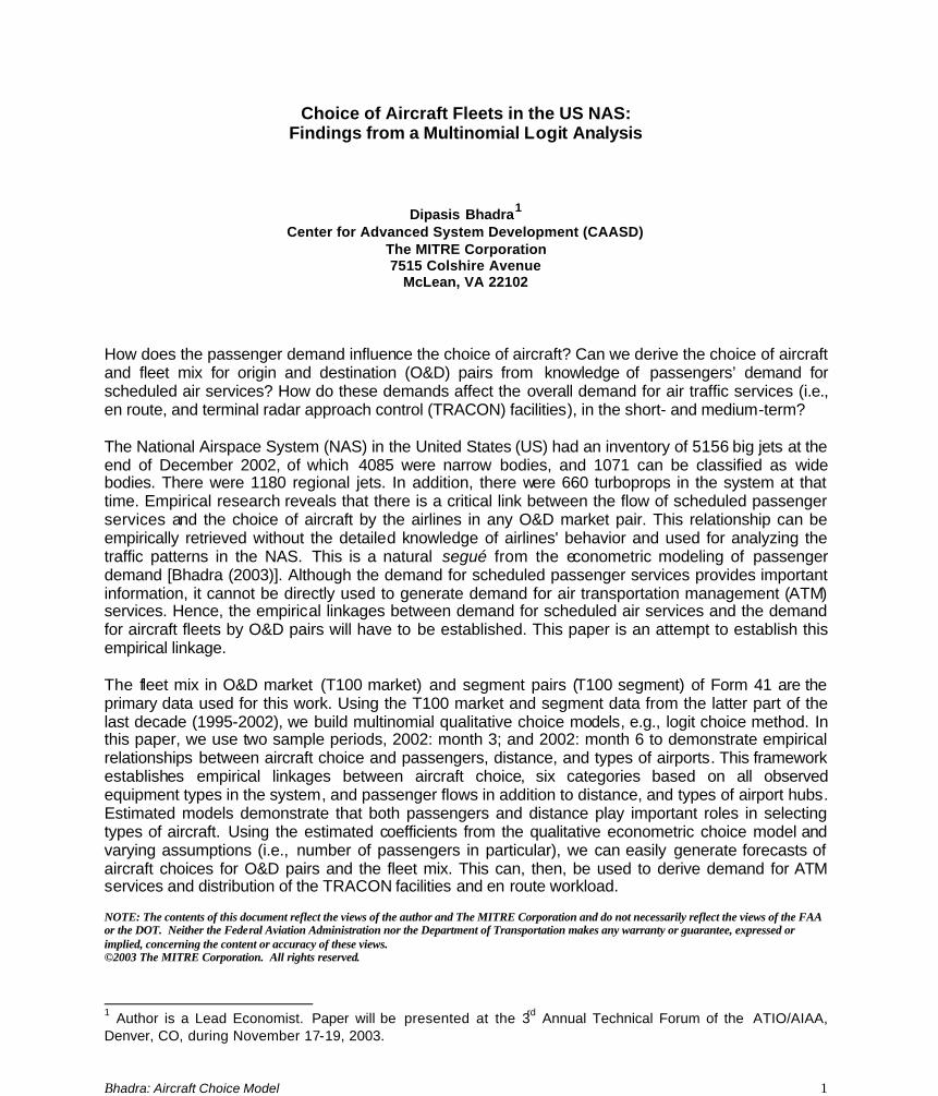
I. Introduction The US airline network is vast. Around 36,000 origin and destination markets are currently served by more than 50,000 flight segments (see Figure 1). Scheduled air carriers transport more than a million passengers undertaking around 15,000 departures a day [see Air Transport Association (ATA) (2003) for aggregate numbers]. This scale of operations is unprecedented in the history of aviation. Scheduling aircraft in a network of this magnitude is understandably a complex task.
34000
35000
36000
37000
38000
39000
40000
41000
42000
1996
:Q1
1996
:Q2
1996:Q
3
1996:Q
4
1997:Q
1
1997:Q
2
1997
:Q3
1997
:Q4
1998
:Q1
1998:Q
2
1998:Q
3
1998
:Q4
1999
:Q1
1999:Q
2
1999:Q
3
1999:Q
4
2000:Q
1
2000
:Q2
2000:Q
3
2000:Q
4
2001:Q
1
2001:Q
2
2001:Q
3
2001
:Q4
2002
:Q1
2002:Q
2year/qtr
O&
D M
arke
t Pai
rs
0
10000
20000
30000
40000
50000
60000
70000
80000
90000
Seg
men
t Pai
rs: T
100
O&D Market Pairs: 10% Data
Segment Pairs: T100
Figure 1: Scheduled Air Services: Market vs. Segment Pairs
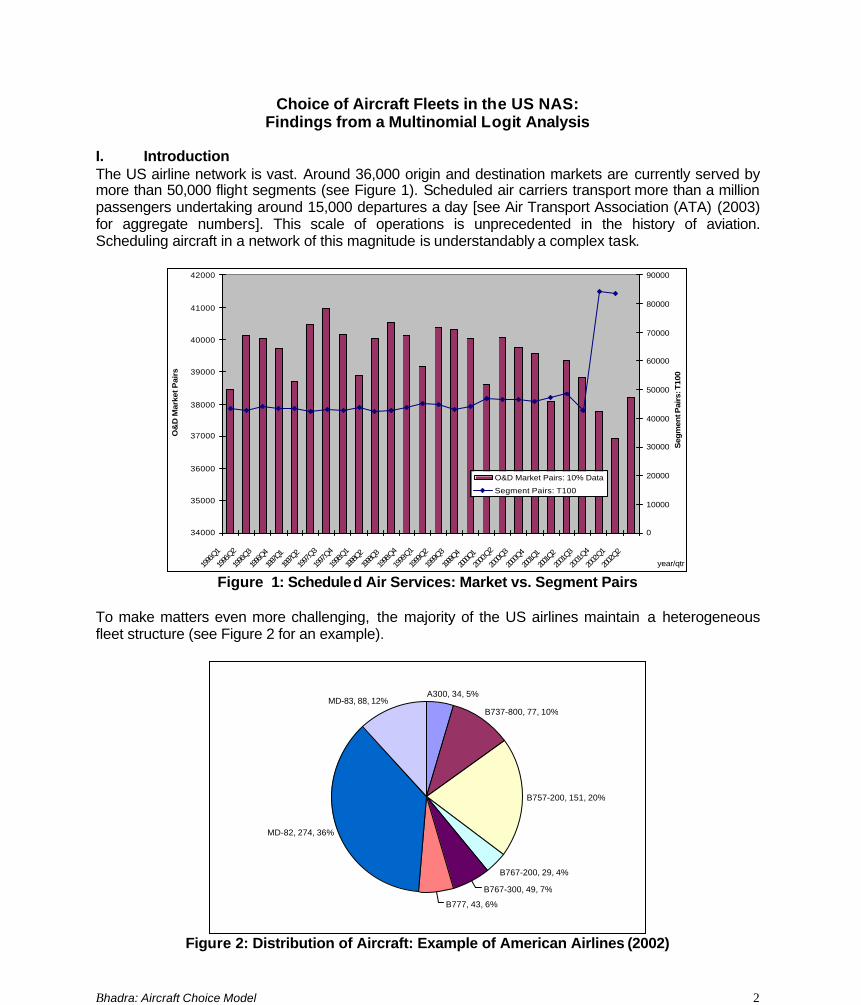
To make matters even more challenging, the majority of the US airlines maintain a heterogeneous fleet structure (see Figure 2 for an example).
A300, 34, 5%
B737-800, 77, 10%
B757-200, 151, 20%
B767-200, 29, 4%
B767-300, 49, 7%
B777, 43, 6%
MD-82, 274, 36%
MD-83, 88, 12%
Figure 2: Distribution of Aircraft: Example of American Airlines (2002)
Bhadra: Aircraft Choice Model 3
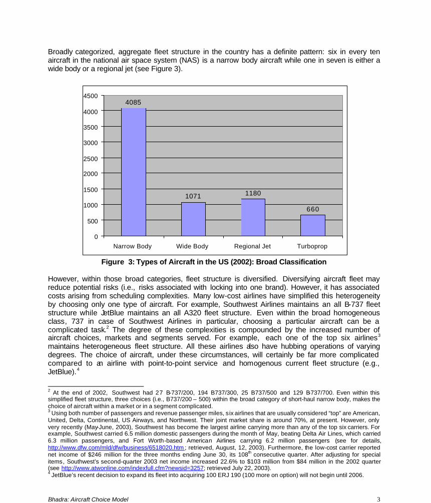
Broadly categorized, aggregate fleet structure in the country has a definite pattern: six in every ten aircraft in the national air space system (NAS) is a narrow body aircraft while one in seven is either a wide body or a regional jet (see Figure 3).
Figure 3: Types of Aircraft in the US (2002): Broad Classification However, within those broad categories, fleet structure is diversified. Diversifying aircraft fleet may reduce potential risks (i.e., risks associated with locking into one brand). However, it has associated costs arising from scheduling complexities. Many low-cost airlines have simplified this heterogeneity by choosing only one type of aircraft. For example, Southwest Airlines maintains an all B-737 fleet structure while JetBlue maintains an all A320 fleet structure. Even within the broad homogeneous class, 737 in case of Southwest Airlines in particular, choosing a particular aircraft can be a complicated task.2 The degree of these complexities is compounded by the increased number of aircraft choices, markets and segments served. For example, each one of the top six airlines3 maintains heterogeneous fleet structure. All these airlines also have hubbing operations of varying degrees. The choice of aircraft, under these circumstances, will certainly be far more complicated compared to an airline with point-to-point service and homogenous current fleet structure (e.g., JetBlue).4
2 At the end of 2002, Southwest had 27 B-737/200, 194 B737/300, 25 B737/500 and 129 B-737/700. Even within this simplified fleet structure, three choices (i.e., B737/200 – 500) within the broad category of short-haul narrow body, makes the choice of aircraft within a market or in a segment complicated. 3 Using both number of passengers and revenue passenger miles, six airlines that are usually considered “top” are American, United, Delta, Continental, US Airways, and Northwest. Their joint market share is around 70%, at present. However, only very recently (May-June, 2003), Southwest has become the largest airline carrying more than any of the top six carriers. For example, Southwest carried 6.5 million domestic passengers during the month of May, beating Delta Air Lines, which carried 6.3 million passengers, and Fort Worth-based American Airlines carrying 6.2 million passengers (see for details, http://www.dfw.com/mld/dfw/business/6518020.htm ; retrieved, August, 12, 2003). Furthermore, the low-cost carrier reported net income of $246 million for the three months ending June 30, its 108th consecutive quarter. After adjusting for special items, Southwest’s second-quarter 2003 net income increased 22.6% to $103 million from $84 million in the 2002 quarter (see http://www.atwonline.com/indexfull.cfm?newsid=3257; retrieved July 22, 2003). 4 JetBlue’s recent decision to expand its fleet into acquiring 100 ERJ 190 (100 more on option) will not begin until 2006.
4085
1071 1180
660
0
500
1000
1500
2000
2500
3000
3500
4000
4500
Narrow Body Wide Body Regional Jet Turboprop
Bhadra: Aircraft Choice Model 4
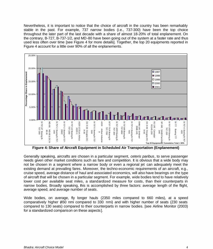
Nevertheless, it is important to notice that the choice of aircraft in the country has been remarkably stable in the past. For example, 737 narrow bodies (i.e., 737-300) have been the top choice throughout the later part of the last decade with a share of almost 18-20% of total enplanement. On the contrary, B-727, B-737-1/2, and MD-80 have been going out of the system at a faster rate and thus used less often over time [see Figure 4 for more details]. Together, the top 20 equipments reported in Figure 4 account for a little over 90% of all the enplanements.
0.00%
5.00%
10.00%
15.00%
20.00%
25.00%
B-737-3/7 B
oeing B-
737-300
MD
-80 MD
-80 & D
C-9-
80 Al
B-757-2 B
oeing B-757-
20
0
B-727-2 B
oeing B-727-
200/2
B-737-1/2 B
oeing B-
737-100/
A320-1/2 E
uro Airbus
A320-1
DC
-9-30 Douglas D
C-
9-30
B-737-5 B
oeing B-737-
50
0
A319 A
irbus IndustrieA
B737-7/LR
Boeing B
-737-700/
B-767-3/E
R B
oeing B-
767-300
B-737-8/9 B
oeing B-
737-800/
B-737-4 B
oeing B-737-
40
0
EM
B-145 E
mbraer
EM
B-145
DC
-9-50 Douglas D
C-
9-50
RJ-145 C
anadairR
J145-200
SF
-340 SA
AB
-Fairchild
34
0
B-767-2/E
R B
oeing B-
767-200
B-777 B
oeing 777
B-767-4 B
oeing B-767-
40
0
Top 20 Equipments' Cumulative Total > 90%
Per
cen
tag
e S
har
e in
En
pla
nem
ent 1997
1998
1999
2000
2001
Figure 4: Share of Aircraft Equipment in Scheduled Air Transportation (Enplanement)
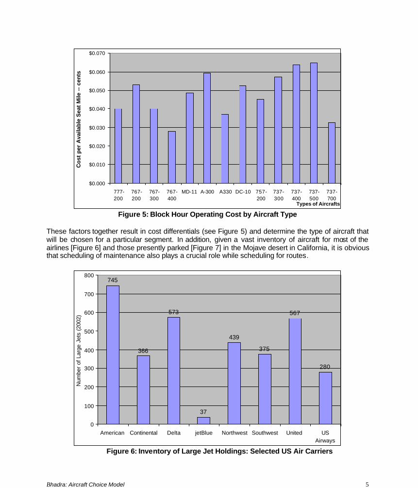
Generally speaking, aircrafts are chosen in a particular segment, ceteris paribus, to serve passenger needs given other market conditions such as fare and competition. It is obvious that a wide body may not be chosen in a segment where a narrow body or even a regional jet can adequately meet the existing demand at prevailing fares. Moreover, the techno-economic requirements of an aircraft, e.g., cruise speed, average distance of haul and associated economics, will also have bearings on the type of aircraft that will be chosen in a particular segment. For example, wide bodies tend to have relatively lower cost per available seat miles, a standardized measure for costs, than their counterparts in narrow bodies. Broadly speaking, this is accomplished by three factors: average length of the flight, average speed, and average number of seats. Wide bodies, on average, fly longer hauls (2350 miles compared to 660 miles), at a speed comparatively higher (450 nmi compared to 330 nmi) and with higher number of seats (230 seats compared to 130 seats) compared to their counterparts in narrow bodies. [see Airline Monitor (2003) for a standardized comparison on these aspects ].
Bhadra: Aircraft Choice Model 5
$0.000
$0.010
$0.020
$0.030
$0.040
$0.050
$0.060
$0.070
777-200
767-200
767-300
767-400
MD-11 A-300 A330 DC-10 757-200
737-300
737-400
737-500
737-700
Types of Aircrafts
Co
st p
er A
vaila
ble
Sea
t M
ile -
- ce
nts
Figure 5: Block Hour Operating Cost by Aircraft Type
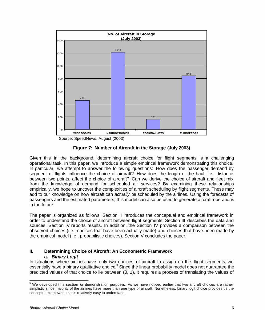
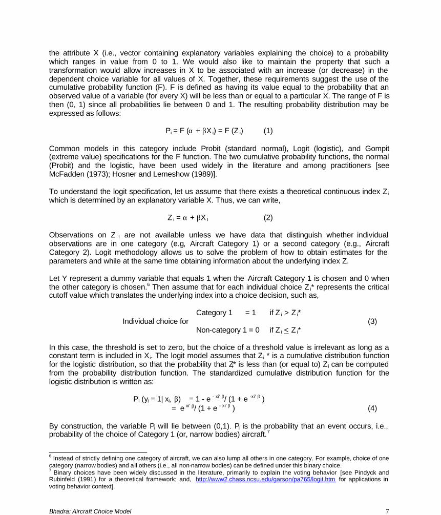
These factors together result in cost differentials (see Figure 5) and determine the type of aircraft that will be chosen for a particular segment. In addition, given a vast inventory of aircraft for most of the airlines [Figure 6] and those presently parked [Figure 7] in the Mojave desert in California, it is obvious that scheduling of maintenance also plays a crucial role while scheduling for routes.
745
366
573
37
439
375
567
280
0
100
200
300
400
500
600
700
800
American Continental Delta jetBlue Northwest Southwest United USAirways
Num
ber
of L
arge
Jet
s (2
002)
Figure 6: Inventory of Large Jet Holdings: Selected US Air Carriers
Bhadra: Aircraft Choice Model 6
No. of Aircraft in Storage (July 2003)
456
1,214
161
843
0
200
400
600
800
1000
1200
1400
WIDE BODIES NARROW BODIES REGIONAL JETS TURBOPROPS Source: SpeedNews, August (2003)
Figure 7: Number of Aircraft in the Storage (July 2003)
Given this in the background, determining aircraft choice for flight segments is a challenging operational task. In this paper, we introduce a simple empirical framework demonstrating this choice. In particular, we attempt to answer the following questions: How does the passenger demand by segment of flights influence the choice of aircraft? How does the length of the haul, i.e., distance between two points, affect the choice of aircraft? Can we derive the choice of aircraft and fleet mix from the knowledge of demand for scheduled air services? By examining these relationships empirically, we hope to uncover the complexities of aircraft scheduling by flight segments. These may add to our knowledge on how aircraft can actually be scheduled by the airlines. Using the forecasts of passengers and the estimated parameters, this model can also be used to generate aircraft operations in the future. The paper is organized as follows: Section II introduces the conceptual and empirical framework in order to understand the choice of aircraft between flight segments; Section III describes the data and sources. Section IV reports results. In addition, the Section IV provides a comparison between the observed choices (i.e., choices that have been actually made) and choices that have been made by the empirical model (i.e., probabilistic choices). Section V concludes the paper. II. Determining Choice of Aircraft: An Econometric Framework
a. Binary Logit In situations where airlines have only two choices of aircraft to assign on the flight segments, we essentially have a binary qualitative choice.5 Since the linear probability model does not guarantee the predicted values of that choice to lie between (0, 1), it requires a process of translating the values of
5 We developed this section for demonstration purposes. As we have noticed earlier that two aircraft choices are rather simplistic since majority of the airlines have more than one type of aircraft. Nonetheless, binary logit choice provides us the conceptual framework that is relatively easy to understand.
Bhadra: Aircraft Choice Model 7
the attribute X (i.e., vector containing explanatory variables explaining the choice) to a probability which ranges in value from 0 to 1. We would also like to maintain the property that such a transformation would allow increases in X to be associated with an increase (or decrease) in the dependent choice variable for all values of X. Together, these requirements suggest the use of the cumulative probability function (F). F is defined as having its value equal to the probability that an observed value of a variable (for every X) will be less than or equal to a particular X. The range of F is then (0, 1) since all probabilities lie between 0 and 1. The resulting probability distribution may be expressed as follows:
Pi = F (α + βX i) = F (Z i) (1) Common models in this category include Probit (standard normal), Logit (logistic), and Gompit (extreme value) specifications for the F function. The two cumulative probability functions, the normal (Probit) and the logistic, have been used widely in the literature and among practitioners [see McFadden (1973); Hosner and Lemeshow (1989)]. To understand the logit specification, let us assume that there exists a theoretical continuous index Z i which is determined by an explanatory variable X. Thus, we can write,
Z i = α + βX I (2) Observations on Z i are not available unless we have data that distinguish whether individual observations are in one category (e.g, Aircraft Category 1) or a second category (e.g., Aircraft Category 2). Logit methodology allows us to solve the problem of how to obtain estimates for the parameters and while at the same time obtaining information about the underlying index Z. Let Y represent a dummy variable that equals 1 when the Aircraft Category 1 is chosen and 0 when the other category is chosen.6 Then assume that for each individual choice Z i* represents the critical cutoff value which translates the underlying index into a choice decision, such as, Category 1 = 1 if Z i > Z i*
Individual choice for (3) Non-category 1 = 0 if Z i < Z i* In this case, the threshold is set to zero, but the choice of a threshold value is irrelevant as long as a constant term is included in X i. The logit model assumes that Z i * is a cumulative distribution function for the logistic distribution, so that the probability that Zi* is less than (or equal to) Z i can be computed from the probability distribution function. The standardized cumulative distribution function for the logistic distribution is written as:
Pi (yi = 1| xi, β) = 1 - e - xi' β/ (1 + e -xi' β ) = e xi' β/ (1 + e - xi' β ) (4)
By construction, the variable Pi will lie between (0,1). Pi is the probability that an event occurs, i.e., probability of the choice of Category 1 (or, narrow bodies) aircraft.7
6 Instead of strictly defining one category of aircraft, we can also lump all others in one category. For example, choice of one category (narrow bodies) and all others (i.e., all non-narrow bodies) can be defined under this binary choice. 7 Binary choices have been widely discussed in the literature, primarily to explain the voting behavior [see Pindyck and Rubinfeld (1991) for a theoretical framework; and, http://www2.chass.ncsu.edu/garson/pa765/logit.htm for applications in voting behavior context].
Bhadra: Aircraft Choice Model 8
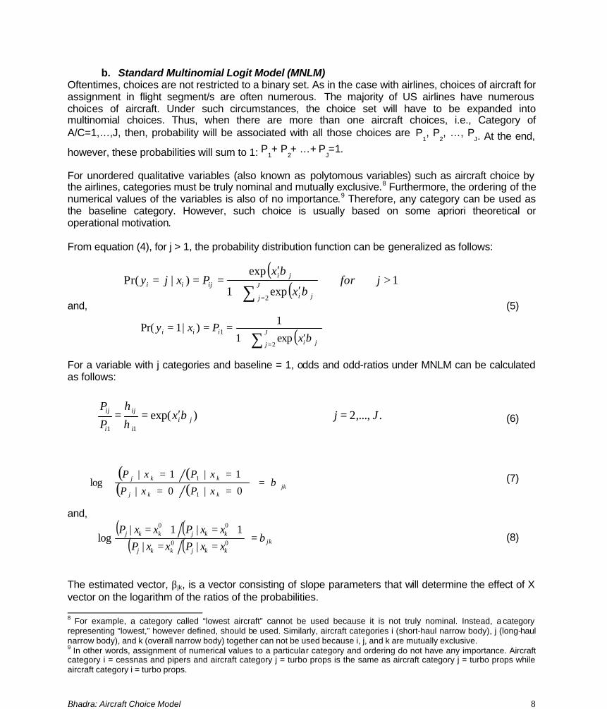
b. Standard Multinomial Logit Model (MNLM) Oftentimes, choices are not restricted to a binary set. As in the case with airlines, choices of aircraft for assignment in flight segment/s are often numerous. The majority of US airlines have numerous choices of aircraft. Under such circumstances, the choice set will have to be expanded into multinomial choices. Thus, when there are more than one aircraft choices, i.e., Category of A/C=1,…,J, then, probability will be associated with all those choices are P
1, P
2, …, P
J. At the end,
however, these probabilities will sum to 1: P1+ P
2+ …+ P
J=1.
For unordered qualitative variables (also known as polytomous variables) such as aircraft choice by the airlines, categories must be truly nominal and mutually exclusive.8 Furthermore, the ordering of the numerical values of the variables is also of no importance.9 Therefore, any category can be used as the baseline category. However, such choice is usually based on some apriori theoretical or operational motivation. From equation (4), for j > 1, the probability distribution function can be generalized as follows: and, (5) For a variable with j categories and baseline = 1, odds and odd-ratios under MNLM can be calculated as follows:
(6) (7) and, (8) The estimated vector, βjk, is a vector consisting of slope parameters that will determine the effect of X vector on the logarithm of the ratios of the probabilities. 8 For example, a category called “lowest aircraft” cannot be used because it is not truly nominal. Instead, a category representing “lowest,” however defined, should be used. Similarly, aircraft categories i (short-haul narrow body), j (long-haul narrow body), and k (overall narrow body) together can not be used because i, j, and k are mutually exclusive. 9 In other words, assignment of numerical values to a particular category and ordering do not have any importance. Aircraft category i = cessnas and pipers and aircraft category j = turbo props is the same as aircraft category j = turbo props while aircraft category i = turbo props.
( )( ) 1
exp1
exp)|Pr(
2
>′+
′===
∑ =
jforx
xPxjy J
j ji
jiijii
β
β
( )∑ =′+
=== J
j ji
iiix
Pxy2
1exp1
1)|1Pr(
β
.,...,2)exp(11
JjxP
Pji
i
ij
i
ij =′== βηη
( ) ( )( ) ( ) jk
kkj
kkj
xPxP
xPxPβ=
==
==
0|0|
1|1|log
1
1
( ) ( )( ) ( ) jk
kkjkkj
kkjkkj
xxPxxPxxPxxP
β=
==+=+=
00
00
||1|1|
log
Bhadra: Aircraft Choice Model 9
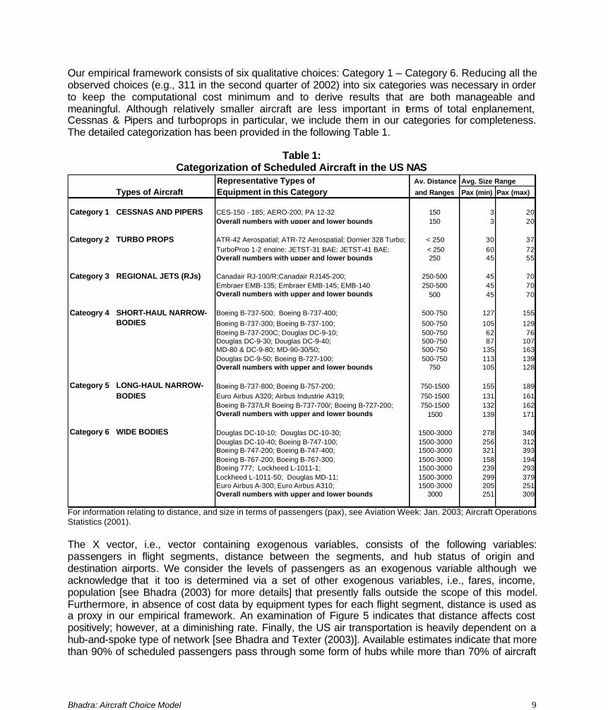
Our empirical framework consists of six qualitative choices: Category 1 – Category 6. Reducing all the observed choices (e.g., 311 in the second quarter of 2002) into six categories was necessary in order to keep the computational cost minimum and to derive results that are both manageable and meaningful. Although relatively smaller aircraft are less important in terms of total enplanement, Cessnas & Pipers and turboprops in particular, we include them in our categories for completeness. The detailed categorization has been provided in the following Table 1.
Table 1: Categorization of Scheduled Aircraft in the US NAS
Representative Types of Av. Distance Avg. Size Range
Types of Aircraft Equipment in this Category and Ranges Pax (min) Pax (max)
Category 1 CESSNAS AND PIPERS CES-150 - 185; AERO-200; PA 12-32 150 3 20Overall numbers with upper and lower bounds 150 3 20
Category 2 TURBO PROPS ATR-42 Aerospatial; ATR-72 Aerospatial; Dornier 328 Turbo; SAAB-Fairchild 340; Embraer EMB-120; < 250 30 37TurboProp 1-2 engine; JETST-31 BAE; JETST-41 BAE; De Havilland DHC 8; < 250 60 72Overall numbers with upper and lower bounds 250 45 55
Category 3 REGIONAL JETS (RJs) Canadair RJ-100/R;Canadair RJ145-200; 250-500 45 70Embraer EMB-135; Embraer EMB-145; EMB-140 Embraer EMB-140; Avroliner RJ85; BAE-146-3; Do328JET;250-500 45 70Overall numbers with upper and lower bounds 500 45 70
Cateogry 4 SHORT-HAUL NARROW- Boeing B-737-500; Boeing B-737-400; 500-750 127 155BODIES Boeing B-737-300; Boeing B-737-100; 500-750 105 129
Boeing B-737-200C; Douglas DC-9-10; 500-750 62 76Douglas DC-9-30; Douglas DC-9-40; 500-750 87 107MD-80 & DC-9-80; MD-90-30/50; 500-750 135 163Douglas DC-9-50; Boeing B-727-100; 500-750 113 139Overall numbers with upper and lower bounds 750 105 128
Category 5 LONG-HAUL NARROW- Boeing B-737-800; Boeing B-757-200; 750-1500 155 189BODIES Euro Airbus A320; Airbus Industrie A319; 750-1500 131 161
Boeing B-737/LR Boeing B-737-700/; Boeing B-727-200; 750-1500 132 162Overall numbers with upper and lower bounds 1500 139 171
Category 6 WIDE BODIES Douglas DC-10-10; Douglas DC-10-30; 1500-3000 278 340Douglas DC-10-40; Boeing B-747-100; 1500-3000 256 312Boeing B-747-200; Boeing B-747-400; 1500-3000 321 393Boeing B-767-200; Boeing B-767-300; 1500-3000 158 194Boeing 777; Lockheed L-1011-1; 1500-3000 239 293Lockheed L-1011-50; Douglas MD-11; 1500-3000 299 379Euro Airbus A-300; Euro Airbus A310; 1500-3000 205 251Overall numbers with upper and lower bounds 3000 251 309
For information relating to distance, and size in terms of passengers (pax), see Aviation Week: Jan. 2003; Aircraft Operations Statistics (2001). The X vector, i.e., vector containing exogenous variables, consists of the following variables: passengers in flight segments, distance between the segments, and hub status of origin and destination airports. We consider the levels of passengers as an exogenous variable although we acknowledge that it too is determined via a set of other exogenous variables, i.e., fares, income, population [see Bhadra (2003) for more details] that presently falls outside the scope of this model. Furthermore, in absence of cost data by equipment types for each flight segment, distance is used as a proxy in our empirical framework. An examination of Figure 5 indicates that distance affects cost positively; however, at a diminishing rate. Finally, the US air transportation is heavily dependent on a hub-and-spoke type of network [see Bhadra and Texter (2003)]. Available estimates indicate that more than 90% of scheduled passengers pass through some form of hubs while more than 70% of aircraft
Bhadra: Aircraft Choice Model 10
operations take place in a hub. Consequently, it is likely that types of hubs may have some impact on types of aircraft that will be chosen to fly a particular segment. Given these, our empirical framework can be specified as follows:
Pi (yi = j| x i, β) = αij + β1 (passengers) + β2 (distance) (j = 1, 2, …, 6) + β3 (OriginHubDummy) + β4 (DestinationHubDummy) + ε i (E.1)
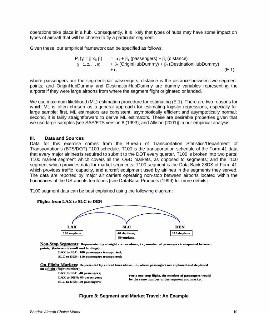
where passengers are the segment-pair passengers; distance is the distance between two segment points; and OriginHubDummy and DestinationHubDummy are dummy variables representing the airports if they were large airports from where the segment flight originated or landed. We use maximum likelihood (ML) estimation procedure for estimating (E.1). There are two reasons for which ML is often chosen as a general approach for estimating logistic regressions, especially for large sample: first, ML estimators are consistent, asymptotically efficient and asymptotically normal; second, it is fairly straightforward to derive ML estimators. These are desirable properties given that we use large samples [see SAS/ETS version 8 (1993); and Allison (2001)] in our empirical analysis. III. Data and Sources Data for this exercise comes from the Bureau of Transportation Statistics/Department of Transportation’s (BTS/DOT) T100 schedule. T100 is the transportation schedule of the Form 41 data that every major airlines is required to submit to the DOT every quarter. T100 is broken into two parts: T100 market segment which covers all the O&D markets, as opposed to segments; and the T100 segment which provides data for market segments. T100 segment is the Data Bank 28DS of Form 41 which provides traffic, capacity, and aircraft equipment used by airlines in the segments they served. The data are reported by major air carriers operating non-stop between airports located within the boundaries of the US and its territories [see DataBase Products (1999) for more details]. T100 segment data can be best explained using the following diagram:
Figure 8: Segment and Market Travel: An Example
LAX SLC DEN
Flights from LAX to SLC to DEN
NonNon--Stop SegmentsStop Segments: Represented by straight arrows above, i.e., number of passengers transported between points, (between take-off and landings).
LAX to SLC: 100 passengers transported; SLC to DEN: 110 passengers transported;
100 enplane 40 deplane; 50 enplane.
110 deplane
OnOn--Flight MarketsFlight Markets: Represented by curved lines above, i.e., where passengers are enplaned and deplaned on a flight (flight number).
LAX to SLC: 40 passengers;LAX to DEN: 60 passengers; SLC to DEN: 50 passengers;
For a one-stop flight, the number of passengers would be the same number under segment and market.
LAX SLC DENLAX SLC DEN
Flights from LAX to SLC to DEN
NonNon--Stop SegmentsStop Segments: Represented by straight arrows above, i.e., number of passengers transported between points, (between take-off and landings).
LAX to SLC: 100 passengers transported; SLC to DEN: 110 passengers transported;
100 enplane 40 deplane; 50 enplane.
110 deplane
OnOn--Flight MarketsFlight Markets: Represented by curved lines above, i.e., where passengers are enplaned and deplaned on a flight (flight number).
LAX to SLC: 40 passengers;LAX to DEN: 60 passengers; SLC to DEN: 50 passengers;
For a one-stop flight, the number of passengers would be the same number under segment and market.
Bhadra: Aircraft Choice Model 11
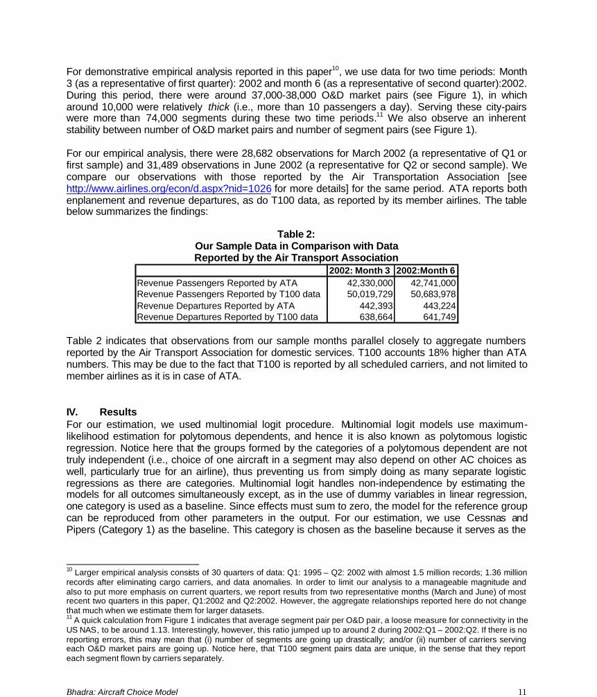
For demonstrative empirical analysis reported in this paper10, we use data for two time periods: Month 3 (as a representative of first quarter): 2002 and month 6 (as a representative of second quarter):2002. During this period, there were around 37,000-38,000 O&D market pairs (see Figure 1), in which around 10,000 were relatively thick (i.e., more than 10 passengers a day). Serving these city-pairs were more than 74,000 segments during these two time periods.11 We also observe an inherent stability between number of O&D market pairs and number of segment pairs (see Figure 1). For our empirical analysis, there were 28,682 observations for March 2002 (a representative of Q1 or first sample) and 31,489 observations in June 2002 (a representative for Q2 or second sample). We compare our observations with those reported by the Air Transportation Association [see http://www.airlines.org/econ/d.aspx?nid=1026 for more details] for the same period. ATA reports both enplanement and revenue departures, as do T100 data, as reported by its member airlines. The table below summarizes the findings:
Table 2: Our Sample Data in Comparison with Data Reported by the Air Transport Association
2002: Month 3 2002:Month 6Revenue Passengers Reported by ATA 42,330,000 42,741,000Revenue Passengers Reported by T100 data 50,019,729 50,683,978Revenue Departures Reported by ATA 442,393 443,224Revenue Departures Reported by T100 data 638,664 641,749
Table 2 indicates that observations from our sample months parallel closely to aggregate numbers reported by the Air Transport Association for domestic services. T100 accounts 18% higher than ATA numbers. This may be due to the fact that T100 is reported by all scheduled carriers, and not limited to member airlines as it is in case of ATA. IV. Results For our estimation, we used multinomial logit procedure. Multinomial logit models use maximum-likelihood estimation for polytomous dependents, and hence it is also known as polytomous logistic regression. Notice here that the groups formed by the categories of a polytomous dependent are not truly independent (i.e., choice of one aircraft in a segment may also depend on other AC choices as well, particularly true for an airline), thus preventing us from simply doing as many separate logistic regressions as there are categories. Multinomial logit handles non-independence by estimating the models for all outcomes simultaneously except, as in the use of dummy variables in linear regression, one category is used as a baseline. Since effects must sum to zero, the model for the reference group can be reproduced from other parameters in the output. For our estimation, we use Cessnas and Pipers (Category 1) as the baseline. This category is chosen as the baseline because it serves as the
10 Larger empirical analysis consists of 30 quarters of data: Q1: 1995 – Q2: 2002 with almost 1.5 million records; 1.36 million records after eliminating cargo carriers, and data anomalies. In order to limit our analysis to a manageable magnitude and also to put more emphasis on current quarters, we report results from two representative months (March and June) of most recent two quarters in this paper, Q1:2002 and Q2:2002. However, the aggregate relationships reported here do not change that much when we estimate them for larger datasets. 11 A quick calculation from Figure 1 indicates that average segment pair per O&D pair, a loose measure for connectivity in the US NAS, to be around 1.13. Interestingly, however, this ratio jumped up to around 2 during 2002:Q1 – 2002:Q2. If there is no reporting errors, this may mean that (i) number of segments are going up drastically; and/or (ii) number of carriers serving each O&D market pairs are going up. Notice here, that T100 segment pairs data are unique, in the sense that they report each segment flown by carriers separately.
Bhadra: Aircraft Choice Model 12
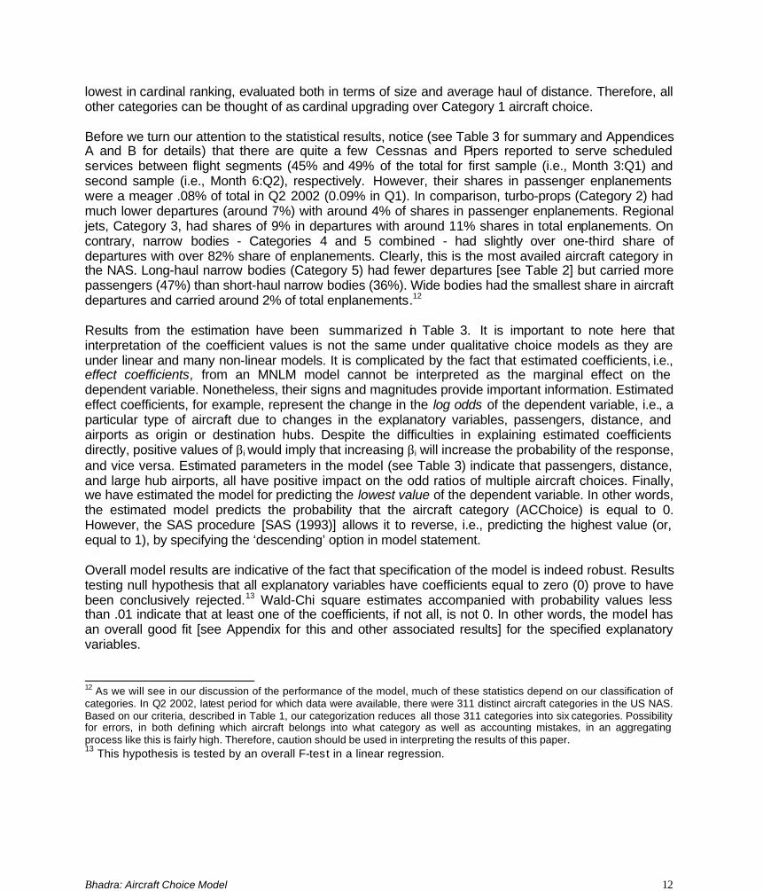
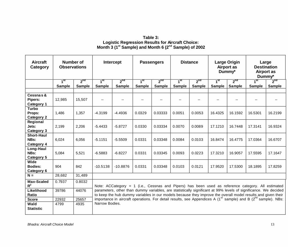
lowest in cardinal ranking, evaluated both in terms of size and average haul of distance. Therefore, all other categories can be thought of as cardinal upgrading over Category 1 aircraft choice. Before we turn our attention to the statistical results, notice (see Table 3 for summary and Appendices A and B for details) that there are quite a few Cessnas and Pipers reported to serve scheduled services between flight segments (45% and 49% of the total for first sample (i.e., Month 3:Q1) and second sample (i.e., Month 6:Q2), respectively. However, their shares in passenger enplanements were a meager .08% of total in Q2 2002 (0.09% in Q1). In comparison, turbo-props (Category 2) had much lower departures (around 7%) with around 4% of shares in passenger enplanements. Regional jets, Category 3, had shares of 9% in departures with around 11% shares in total enplanements. On contrary, narrow bodies - Categories 4 and 5 combined - had slightly over one-third share of departures with over 82% share of enplanements. Clearly, this is the most availed aircraft category in the NAS. Long-haul narrow bodies (Category 5) had fewer departures [see Table 2] but carried more passengers (47%) than short-haul narrow bodies (36%). Wide bodies had the smallest share in aircraft departures and carried around 2% of total enplanements.12 Results from the estimation have been summarized in Table 3. It is important to note here that interpretation of the coefficient values is not the same under qualitative choice models as they are under linear and many non-linear models. It is complicated by the fact that estimated coefficients, i.e., effect coefficients, from an MNLM model cannot be interpreted as the marginal effect on the dependent variable. Nonetheless, their signs and magnitudes provide important information. Estimated effect coefficients, for example, represent the change in the log odds of the dependent variable, i.e., a particular type of aircraft due to changes in the explanatory variables, passengers, distance, and airports as origin or destination hubs. Despite the difficulties in explaining estimated coefficients directly, positive values of βi would imply that increasing βi will increase the probability of the response, and vice versa. Estimated parameters in the model (see Table 3) indicate that passengers, distance, and large hub airports, all have positive impact on the odd ratios of multiple aircraft choices. Finally, we have estimated the model for predicting the lowest value of the dependent variable. In other words, the estimated model predicts the probability that the aircraft category (ACChoice) is equal to 0. However, the SAS procedure [SAS (1993)] allows it to reverse, i.e., predicting the highest value (or, equal to 1), by specifying the ‘descending’ option in model statement. Overall model results are indicative of the fact that specification of the model is indeed robust. Results testing null hypothesis that all explanatory variables have coefficients equal to zero (0) prove to have been conclusively rejected.13 Wald-Chi square estimates accompanied with probability values less than .01 indicate that at least one of the coefficients, if not all, is not 0. In other words, the model has an overall good fit [see Appendix for this and other associated results] for the specified explanatory variables. 12 As we will see in our discussion of the performance of the model, much of these statistics depend on our classification of categories. In Q2 2002, latest period for which data were available, there were 311 distinct aircraft categories in the US NAS. Based on our criteria, described in Table 1, our categorization reduces all those 311 categories into six categories. Possibility for errors, in both defining which aircraft belongs into what category as well as accounting mistakes, in an aggregating process like this is fairly high. Therefore, caution should be used in interpreting the results of this paper. 13 This hypothesis is tested by an overall F-test in a linear regression.
Bhadra: Aircraft Choice Model 13
Table 3:
Logistic Regression Results for Aircraft Choice: Month 3 (1st Sample) and Month 6 (2nd Sample) of 2002
Aircraft Category
Number of
Observations
Intercept
Passengers
Distance
Large Origin
Airport as Dummy*
Large
Destination Airport as Dummy*
1st Sample
2nd Sample
1st Sample
2nd Sample
1st Sample
2nd Sample
1st Sample
2nd Sample
1st Sample
2nd Sample
1st Sample
2nd Sample
Cessna s & Pipers: Category 1
12,985
15,507
--
--
--
--
--
--
--
--
--
--
Turbo Props: Category 2
1,486
1,357
-4.3199
-4.4936
0.0329
0.03333
0.0051
0.0053
16.4325
16.1592
16.5301
16.2199
Regional Jets: Category 3
2,199
2,206
-5.4433
-5.8727
0.0330
0.03334
0.0070
0.0089
17.1210
16.7448
17.3141
16.9324
Short-Haul NBs: Category 4
6,024
6,056
-5.1151
-5.5509
0.0331
0.03348
0.0084
0.0103
16.8474
16.4775
17.0364
16.6707
Long-Haul NBs: Category 5
5,084
5,521
-6.5883
-6.8227
0.0331
0.03345
0.0093
0.0223
17.3210
16.9057
17.5595
17.1647
Wide Bodies: Category 6
904
842
-10.5138
-10.8876
0.0331
0.03348
0.0103
0.0121
17.9520
17.5300
18.1895
17.8259
N = 28,682 31,489
Max-Scaled R2
0.7937 0.8032
Likelihood Ratio
39786 44076
Score 22932 25657 Wald Statistic
4799 4935
Note: ACCategory = 1 (i.e., Cessnas and Pipers) has been used as reference category. All estimated parameters, other than dummy variables, are statistically significant at 99% levels of significance. We decided to keep the hub dummy variables in our models because they improve the overall model results and given their importance in aircraft operations. For detail results, see Appendices A (1st sample) and B (2nd sample). NBs: Narrow Bodies.
Having observed these aggregate statistics, we also notice that the estimated parameters are all statistically significant, except the hub status of both origin and destination airports. In order to save space, we report only estimated parameters, and not the Wald Chi-Squares.14 Wald chi-squares are calculated by dividing each coefficient by its standard error and squaring the result.15
Table 4: Performance of the Model: Actual vs. Predicted
AC Category
Actual Choice
“Exact” Predicted Response
“One-Off” Predicted Response
3rd Month:Q1
6th Month:Q2
Q1 Q2 Q1 Q2
Cessna s and Pipers:
Category 1
12,985
15,507
12,933 (99.60)
15,442 (99.58)
12,950 (99.73)
15,463 (99.72)
Turbo Props: Category 2
1,486
1,357
76
(5.11)
113
(8.33)
467
(31.43)
483
(35.59) Regional Jets:
Category 3
2,199
2,206 4
(0.18)
7
(0.32)
1,977
(89.90)
1,895
(85.90) Short-Haul NBs:
Category 4
6,024
6,056
4,235 (70.30)
3,975
(65.64)
5,756
(95.55)
5,787
(95.56) Long-Haul NBs:
Category 5
5,084
5,521
2,529 (49.74)
2,908
(52.67)
4,814
(94.69)
5,187
(93.95)
Wide Bodies: Category 6
904
842
51
(5.64)
33
(3.92)
703
(77.77)
637
(75.65) N / Average % of Correct Response
28,682
31,489
38.42
38.41
81.52
81.06
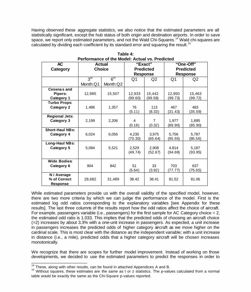
While estimated parameters provide us with the overall validity of the specified model, however, there are two more criteria by which we can judge the performance of the model. First is the estimated log odd ratios corresponding to the explanatory variables [see Appendix for these results]. The last three columns of the results report how the odd ratios affect the choice of aircraft. For example, passengers variable (i.e., passengers) for the first sample for AC Category choice = 2, the estimated odd ratio is 1.033. This implies that the predicted odds of choosing an aircraft choice (=2) increases by about 3.3% with a one-unit increase in passengers. As expected, a unit increase in passengers increases the predicted odds of higher category aircraft as we move higher on the cardinal scale. This is most clear with the distance as the independent variable; with a unit increase in distance (i.e., a mile), predicted odds that a higher category aircraft will be chosen increases monotonically. We recognize that there are scopes for further model improvement. Instead of working on those developments, we decided to use the estimated parameters to predict the responses in order to 14 These, along with other results, can be found in attached Appendices A and B. 15 Without squares, these estimates are the same as t or z statistics. The p-values calculated from a normal table would be exactly the same as the Chi-Square p-values reported.
Bhadra: Aircraft Choice Model 15
evaluate the model’s performance as it stand now. We compare these predicted responses against that of actual choices. Actual choices have been reported in Column 1. When predicted responses matched “exactly” to that of actual, we call them “exact” predicted responses, as reported in Column 2.16 When the exactness is made somewhat flexible, and we allow one choice + in the category, we arrive at predicted responses that are “one-off” (reported in Column 3). For example, when the choice of an aircraft (say, for example, Aircraft Category = 4) can have a value of both 3 and 5, in addition to its exact value of 3, we call this as “one-off” predicted response.17 We created this category in order to account for the fact that often choice of aircraft is not clearly distinct as implied by the categorical cardinal choice of 1, 2, …, 6. Furthermore, this flexibility allows the model to be more useful for operations. Table 4 summarizes these results. As expected, flexibility allows for a better fit. For both the samples, one-off predicted responses coming out of our models match with actual choice approximately 81% [see the last row of the last two columns of Table 4]. In other words, the estimated model with one-off allowance is capable of explaining 81% of the actual aircraft choice sample. However, this fit drops to almost half when we look at the “exact” match. For both the samples, we are not able to explain more than 38% of the actual aircraft choices. Generally speaking, estimated models appear to be good fit for aircraft choices 1, 4, and 5 when evaluated against the actual choices, and have poorer fit for other choices. In fact, our model is a rather poor fit for the choice of regional jets (ACChoice = 3) and somewhat weak for choices of turbo-props (ACChoice = 2) and wide bodies (ACChoice = 6). Finally, the predictability of the model improves significantly when we allow one-off responses in lieu of exact. Interestingly, however, the gain is somewhat small for the aircraft choice = 2 (i.e., Turbo Props) when we move from the exact to one-off possibilities. V. Conclusion In this paper, we have used a multinomial logistic regression model to determine the choice of aircraft in the US NAS. By categorizing all aircrafts into 6 categories, we have found that passengers, distance, and types of airport hubs are capable of estimating these choices fairly well. Our preliminary findings indicate that estimated model is capable of explaining these choices exactly for 3 particular aircraft types. Almost all aircraft choices can be explained if we allow one-off predicted responses in place of exact predicted response. These findings have important implications. First, we are now capable of mapping passengers onto aircraft choices, given distance and the status of hubs through these estimated models. This provides us with another tool, similar to terminal area estimates and forecasts. Second and most importantly, this correspondence allows us to generate schedules or timetable specific to airports allowing us to simulate the US NAS far more efficiently than we were capable of before. There are quite a few areas of future research that we plan to pursue in the near future. First, we plan to segment the data by distance categories, i.e., short haul (< 750 miles), medium haul (750-1500 miles) and long haul (> 1500 miles) and reestimate our model. This may improve the results because choices will be weighted by the haul of distances they fly. This added information may benefit the estimation substantially. Second, the above model does not consider airline behaviors in aircraft choice. By incorporating airline-specific behaviors explicitly, we hope to improve the above model. Third, passenger demand can be modeled “nested” in our model. Passenger demand that is determined by economic factors can be modeled nested inside as determinants of aircraft choice.
16 Numbers in parentheses represent percentage of predicted responses that are “right” in comparison to actuals. 17 Notice, however, that the tail is cut in half for the first and last choices, for there is no choice less than aircraft choice = 1; and no choice greater than aircraft choice = 6 in our specification.
Bhadra: Aircraft Choice Model 16
REFERENCES Airline Monitor (2003). “Block Hour Operating Costs by Airplane Type for the Year 2002”, August, Part II. Air Transport Association (2003). See http://www.airlines.org/public/home/default1.asp. Allison, P.D. (2001). Logistic Regression Using the SAS System: Theory and Application, SAS Institute. Aviation Week & Space Technology (2003). “Aerospace Source Book, January 13th issue. Bhadra, D. (2003). “Demand for Air Travel in the United States: Bottom-Up Econometric Estimation and Implications for Forecasts by O&D Pairs,” Journal of Air Transportation, September, Vol. 8, No. 2. __, and P.A. Texter (2003). “Changing Network: A Time Series Analysis of US Domestic Air
Travel”, Paper presented at the Forecasting in Transportation session of the 23rd International Symposium on Forecasting, Mérida, Mexico, June 15-18, 2003. Database Products, Inc. (1999). “O&D Mannual,” Texas. Hosner, D.W. and S. Lemeshow (1989). Applied Logistic Regression. New York: John Wiley & Sons. McFadden, D. (1973). “Conditional Logit Analysis of Qualitative Choice Behavior,” in Frontiers in Econometrics, ed. By P. Zarembka, New York: Academic Press, pp. 105-142. Pindyck, R.S. and D.L. Rubinfeld (1991). Econometric Models and Economic Forecasts , 3rd Edition, New York: McGraw-Hill, Inc. SAS/ETS Software (1993). Applications Guide 2: Econometric Modeling, Simulation, and Forecasting, Version 6, First Edition, SAS Institute, Cary, NC. SAS Institute Inc. (1995). Logistic Regression Examples Using the SAS System . Cary, NC.
Bhadra: Aircraft Choice Model 17
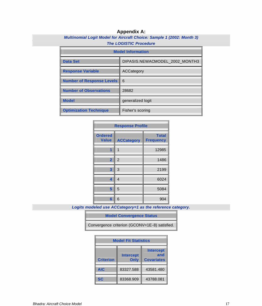
Appendix A: Multinomial Logit Model for Aircraft Choice: Sample 1 (2002: Month 3)
The LOGISTIC Procedure
Model Information
Data Set DIPASIS.NEWACMODEL_2002_MONTH3
Response Variable ACCategory
Number of Response Levels 6
Number of Observations 28682
Model generalized logit
Optimization Technique Fisher's scoring
Response Profile
Ordered Value ACCategory
Total Frequency
1 1 12985
2 2 1486
3 3 2199
4 4 6024
5 5 5084
6 6 904
Logits modeled use ACCategory=1 as the reference category.
Model Convergence Status
Convergence criterion (GCONV=1E-8) satisfied.
Model Fit Statistics
Criterion Intercept
Only
Intercept and
Covariates
AIC 83327.588 43581.480
SC 83368.909 43788.081

Bhadra: Aircraft Choice Model 18
Model Fit Statistics
Criterion Intercept
Only
Intercept and
Covariates
-2 Log L 83317.588 43531.480
R-Square 0.7502 Max-rescaled R-Square 0.7937
Testing Global Null Hypothesis: BETA=0
Test Chi-Square DF Pr > ChiSq
Likelihood Ratio 39786.1083 20 <.0001
Score 22932.2618 20 <.0001
Wald 4798.9823 20 <.0001
Type III Analysis of Effects
Effect DF Wald
Chi-Square Pr > ChiSq
PASSENGERS 5 704.2160 <.0001
DISTANCE 5 3232.3372 <.0001
LARGEHUBORIGINairpor 5 293.6393 <.0001
LARGEHUBDESTairport 5 362.9332 <.0001
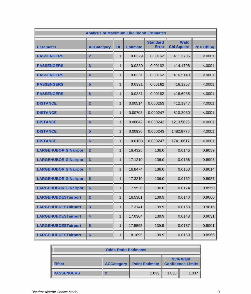
Analysis of Maximum Likelihood Estimates
Parameter ACCategory DF Estimate Standard
Error Wald
Chi-Square Pr > ChiSq
Intercept 2 1 -4.3199 0.0617 4906.4266 <.0001
Intercept 3 1 -5.4433 0.0722 5684.2009 <.0001
Intercept 4 1 -5.1151 0.0655 6096.7059 <.0001
Intercept 5 1 -6.5883 0.0750 7715.9951 <.0001
Intercept 6 1 -10.5138 0.1462 5172.8407 <.0001
Bhadra: Aircraft Choice Model 19
Analysis of Maximum Likelihood Estimates
Parameter ACCategory DF Estimate Standard
Error Wald
Chi-Square Pr > ChiSq
PASSENGERS 2 1 0.0329 0.00162 411.2706 <.0001
PASSENGERS 3 1 0.0330 0.00162 414.1798 <.0001
PASSENGERS 4 1 0.0331 0.00162 416.5140 <.0001
PASSENGERS 5 1 0.0331 0.00162 416.1257 <.0001
PASSENGERS 6 1 0.0331 0.00162 416.6935 <.0001
DISTANCE 2 1 0.00514 0.000253 412.1347 <.0001
DISTANCE 3 1 0.00703 0.000247 810.3030 <.0001
DISTANCE 4 1 0.00842 0.000242 1213.5626 <.0001
DISTANCE 5 1 0.00936 0.000243 1482.8778 <.0001
DISTANCE 6 1 0.0103 0.000247 1741.6617 <.0001
LARGEHUBORIGINairpor 2 1 16.4325 136.0 0.0146 0.9039
LARGEHUBORIGINairpor 3 1 17.1210 136.0 0.0158 0.8998
LARGEHUBORIGINairpor 4 1 16.8474 136.0 0.0153 0.9014
LARGEHUBORIGINairpor 5 1 17.3210 136.0 0.0162 0.8987
LARGEHUBORIGINairpor 6 1 17.9520 136.0 0.0174 0.8950
LARGEHUBDESTairport 2 1 16.5301 139.9 0.0140 0.9060
LARGEHUBDESTairport 3 1 17.3141 139.9 0.0153 0.9015
LARGEHUBDESTairport 4 1 17.0364 139.9 0.0148 0.9031
LARGEHUBDESTairport 5 1 17.5595 139.9 0.0157 0.9001
LARGEHUBDESTairport 6 1 18.1895 139.9 0.0169 0.8966
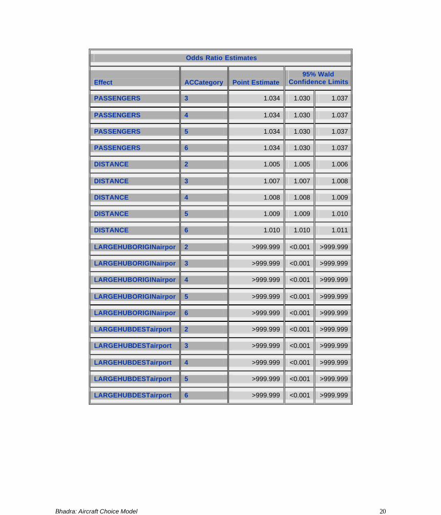
Odds Ratio Estimates
Effect ACCategory Point Estimate 95% Wald
Confidence Limits
PASSENGERS 2 1.033 1.030 1.037
Bhadra: Aircraft Choice Model 20
Odds Ratio Estimates
Effect ACCategory Point Estimate 95% Wald
Confidence Limits
PASSENGERS 3 1.034 1.030 1.037
PASSENGERS 4 1.034 1.030 1.037
PASSENGERS 5 1.034 1.030 1.037
PASSENGERS 6 1.034 1.030 1.037
DISTANCE 2 1.005 1.005 1.006
DISTANCE 3 1.007 1.007 1.008
DISTANCE 4 1.008 1.008 1.009
DISTANCE 5 1.009 1.009 1.010
DISTANCE 6 1.010 1.010 1.011
LARGEHUBORIGINairpor 2 >999.999 <0.001 >999.999
LARGEHUBORIGINairpor 3 >999.999 <0.001 >999.999
LARGEHUBORIGINairpor 4 >999.999 <0.001 >999.999
LARGEHUBORIGINairpor 5 >999.999 <0.001 >999.999
LARGEHUBORIGINairpor 6 >999.999 <0.001 >999.999
LARGEHUBDESTairport 2 >999.999 <0.001 >999.999
LARGEHUBDESTairport 3 >999.999 <0.001 >999.999
LARGEHUBDESTairport 4 >999.999 <0.001 >999.999
LARGEHUBDESTairport 5 >999.999 <0.001 >999.999
LARGEHUBDESTairport 6 >999.999 <0.001 >999.999
Bhadra: Aircraft Choice Model 21
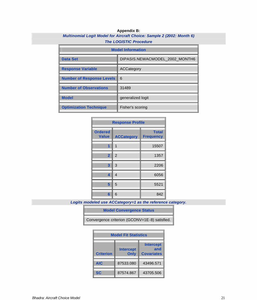
Appendix B: Multinomial Logit Model for Aircraft Choice: Sample 2 (2002: Month 6)
The LOGISTIC Procedure
Model Information
Data Set DIPASIS.NEWACMODEL_2002_MONTH6
Response Variable ACCategory
Number of Response Levels 6
Number of Observations 31489
Model generalized logit
Optimization Technique Fisher's scoring
Response Profile
Ordered Value ACCategory
Total Frequency
1 1 15507
2 2 1357
3 3 2206
4 4 6056
5 5 5521
6 6 842
Logits modeled use ACCategory=1 as the reference category.
Model Convergence Status
Convergence criterion (GCONV=1E-8) satisfied.
Model Fit Statistics
Criterion Intercept
Only
Intercept and
Covariates
AIC 87533.080 43496.571
SC 87574.867 43705.506
Bhadra: Aircraft Choice Model 22
Model Fit Statistics
Criterion Intercept
Only
Intercept and
Covariates
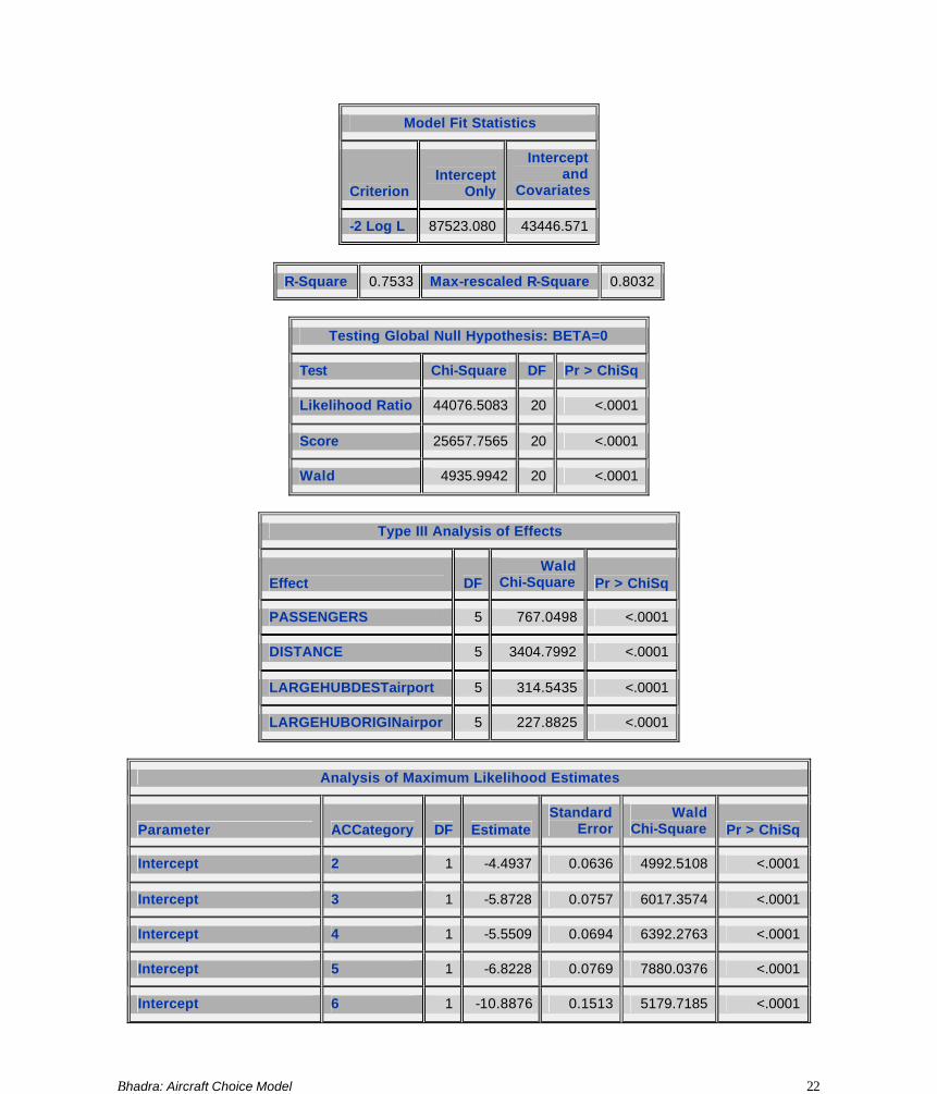
-2 Log L 87523.080 43446.571
R-Square 0.7533 Max-rescaled R-Square 0.8032
Testing Global Null Hypothesis: BETA=0
Test Chi-Square DF Pr > ChiSq
Likelihood Ratio 44076.5083 20 <.0001
Score 25657.7565 20 <.0001
Wald 4935.9942 20 <.0001
Type III Analysis of Effects
Effect DF Wald
Chi-Square Pr > ChiSq
PASSENGERS 5 767.0498 <.0001
DISTANCE 5 3404.7992 <.0001
LARGEHUBDESTairport 5 314.5435 <.0001
LARGEHUBORIGINairpor 5 227.8825 <.0001
Analysis of Maximum Likelihood Estimates
Parameter ACCategory DF Estimate Standard
Error Wald
Chi-Square Pr > ChiSq
Intercept 2 1 -4.4937 0.0636 4992.5108 <.0001
Intercept 3 1 -5.8728 0.0757 6017.3574 <.0001
Intercept 4 1 -5.5509 0.0694 6392.2763 <.0001
Intercept 5 1 -6.8228 0.0769 7880.0376 <.0001
Intercept 6 1 -10.8876 0.1513 5179.7185 <.0001

Bhadra: Aircraft Choice Model 23
Analysis of Maximum Likelihood Estimates
Parameter ACCategory DF Estimate Standard
Error Wald
Chi-Square Pr > ChiSq
PASSENGERS 2 1 0.0333 0.00148 503.9285 <.0001
PASSENGERS 3 1 0.0334 0.00148 506.7413 <.0001
PASSENGERS 4 1 0.0335 0.00148 509.3486 <.0001
PASSENGERS 5 1 0.0335 0.00148 508.3604 <.0001
PASSENGERS 6 1 0.0335 0.00148 509.3531 <.0001
DISTANCE 2 1 0.00535 0.000296 326.4060 <.0001
DISTANCE 3 1 0.00891 0.000279 1018.3612 <.0001
DISTANCE 4 1 0.0103 0.000275 1409.0377 <.0001
DISTANCE 5 1 0.0112 0.000276 1655.9940 <.0001
DISTANCE 6 1 0.0121 0.000280 1874.9133 <.0001
LARGEHUBDESTairport 2 1 16.2200 132.7 0.0149 0.9027
LARGEHUBDESTairport 3 1 16.9325 132.7 0.0163 0.8985
LARGEHUBDESTairport 4 1 16.6708 132.7 0.0158 0.9000
LARGEHUBDESTairport 5 1 17.1647 132.7 0.0167 0.8971
LARGEHUBDESTairport 6 1 17.8259 132.7 0.0180 0.8931
LARGEHUBORIGINairpor 2 1 16.1592 127.9 0.0160 0.8994
LARGEHUBORIGINairpor 3 1 16.7448 127.9 0.0171 0.8958
LARGEHUBORIGINairpor 4 1 16.4775 127.9 0.0166 0.8975
LARGEHUBORIGINairpor 5 1 16.9058 127.9 0.0175 0.8948
LARGEHUBORIGINairpor 6 1 17.5301 127.9 0.0188 0.8910
Odds Ratio Estimates
Effect ACCategory Point Estimate 95% Wald
Confidence Limits
PASSENGERS 2 1.034 1.031 1.037
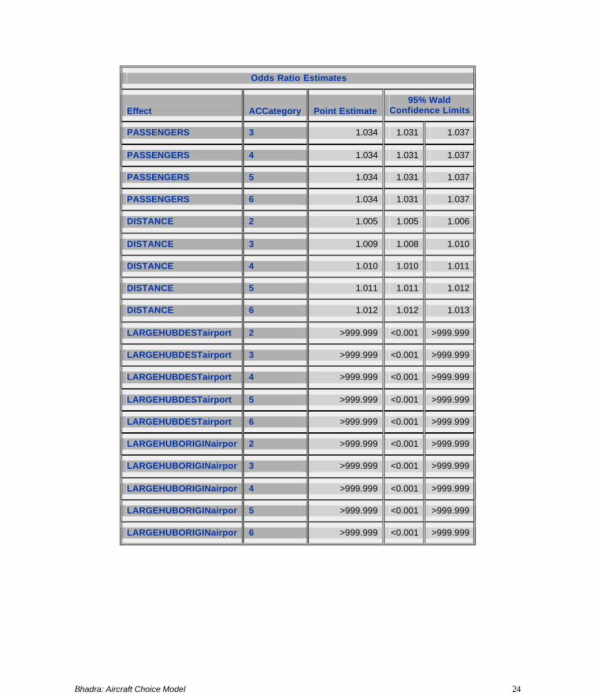
Bhadra: Aircraft Choice Model 24
Odds Ratio Estimates
Effect ACCategory Point Estimate 95% Wald
Confidence Limits
PASSENGERS 3 1.034 1.031 1.037
PASSENGERS 4 1.034 1.031 1.037
PASSENGERS 5 1.034 1.031 1.037
PASSENGERS 6 1.034 1.031 1.037
DISTANCE 2 1.005 1.005 1.006
DISTANCE 3 1.009 1.008 1.010
DISTANCE 4 1.010 1.010 1.011
DISTANCE 5 1.011 1.011 1.012
DISTANCE 6 1.012 1.012 1.013
LARGEHUBDESTairport 2 >999.999 <0.001 >999.999
LARGEHUBDESTairport 3 >999.999 <0.001 >999.999
LARGEHUBDESTairport 4 >999.999 <0.001 >999.999
LARGEHUBDESTairport 5 >999.999 <0.001 >999.999
LARGEHUBDESTairport 6 >999.999 <0.001 >999.999
LARGEHUBORIGINairpor 2 >999.999 <0.001 >999.999
LARGEHUBORIGINairpor 3 >999.999 <0.001 >999.999
LARGEHUBORIGINairpor 4 >999.999 <0.001 >999.999
LARGEHUBORIGINairpor 5 >999.999 <0.001 >999.999
LARGEHUBORIGINairpor 6 >999.999 <0.001 >999.999