Embed Size (px)
Citation preview
JHEP10(2013)186
Published for SISSA by Springer
Received: September 3, 2013
Accepted: September 22, 2013
Published: October 29, 2013
Chiral conductivities and effective field theory
Kristan Jensen, Pavel Kovtun and Adam Ritz
Department of Physics and Astronomy, University of Victoria,
Victoria, BC V8W 3P6, Canada
E-mail: [email protected], [email protected], [email protected]
Abstract: We construct the three-dimensional effective field theory which reproduces
low-momentum static correlation functions in four-dimensional quantum field theories with
U(1) axial anomalies and a dynamical vector gauge field, in thermal equilibrium. We com-
pute radiative corrections to parity-violating chiral conductivities, to leading order in the
effective theory. All of the anomaly-induced transport is susceptible to radiative correc-
tions, except for certain two-point functions which are required by symmetry to vanish.
Keywords: Anomalies in Field and String Theories, Holography and quark-gluon plas-
mas, Global Symmetries
ArXiv ePrint: 1307.3234
c© SISSA 2013 doi:10.1007/JHEP10(2013)186
JHEP10(2013)186
Contents
1 Introduction and summary 1
1.1 Introduction 1
1.2 Summary 3
2 Non-dynamical background fields 8
2.1 Anomalous conservation laws 8
2.2 Anomalous hydrodynamics 12
2.3 Anomalous hydrostatics 15
3 Weak gauging and dynamical photons 21
3.1 Anomalous conservation laws 21
3.2 Anomalous (magneto-)hydrodynamics 22
3.3 Anomalous (magneto-)hydrostatics 24
3.3.1 The (magneto-)hydrostatic effective theory 24
3.3.2 The thermal effective action and chiral conductivities 28
4 Perturbative corrections to chiral correlators 34
4.1 Feynman rules 35
4.2 Perturbative computations 37
4.2.1 Corrections to χ0 38
4.2.2 Corrections to ϕAA 40
4.2.3 Corrections to ϕAV 40
4.2.4 Corrections to ϕAa 40
4.2.5 Summary of the one-loop corrections 41
4.3 Matching to the four-dimensional theory 41
5 Discussion 44
1 Introduction and summary
1.1 Introduction
Anomalies are a ubiquitous feature of quantum field theories. Their usefulness is tied to the
fact that they are exact and so may be determined even at strong coupling. This exactness
is a consequence of certain non-renormalization properties, and allows non-perturbative
insight via tools such as anomaly matching [1]. There has been a recent resurgence of
interest in anomalies in the context of field theory at nonzero temperature and chemical
potential. In particular, it is now known that in the hydrodynamic limit there are certain
– 1 –
JHEP10(2013)186
first-order transport coefficients, on the same footing as viscosity or conductivity, which
are fixed in terms of anomaly coefficients and thermodynamic quantities [2–5].
Such anomaly-induced transport is dissipationless, as may be seen by an entropy pro-
duction analysis within hydrodynamics. In addition, the corresponding transport coef-
ficients are determined by Euclidean Kubo formulae [6], meaning that they are thermo-
dynamic parameters, and may be measured in equilibrium. Thanks to their thermody-
namic nature, the anomalous transport coefficients can also be understood from Euclidean
field theory [7, 8]. This anomaly-induced hydrodynamic transport provides a macroscopic
manifestation of microscopic anomaly-induced physics, such as the chiral magnetic ef-
fect (CME) [9–12], chiral separation effect (CSE) [13–15], and the chiral vortical effect
(CVE) [16]. Specifically, for a theory with a vector current JµV,cov and an axial current
JµA,cov, coupled to the corresponding background non-dynamical sources Vµ and Aµ, anoma-
lies give rise to the following additional terms in the hydrodynamic constitutive relations:
JµV,cov = · · ·+ ξV wµ + ξV VB
µ + ξV ABµA ,
JµA,cov = · · ·+ ξAwµ + ξAVB
µ + ξAABµA .
(1.1)
Here uµ is the fluid velocity, Bµ = 12εµνρσuνFV,ρσ, and Bµ
A = 12εµνρσuνFA,ρσ are the cor-
responding vector and axial magnetic fields, and wµ = εµνρσuν∇ρuσ is the vorticity. The
subscript denotes covariant currents, as we explain later. The CME is usually associated
with the ξV V term, the CSE with the ξAV term and the CVE with the ξA term. See [17]
for a recent review.
Most of the results on anomalous transport are derived for theories whose anomalies
involve only global symmetries. In this case, if we schematically denote the anomalous
current divergence as ∇JA = cF F , the background field strength on the right-hand side
is non-dynamical, the symmetry currents are non-perturbatively defined objects, and the
corresponding anomalies are exact: under an anomalous background gauge transformation,
the partition function picks up a definite, anomalous phase which is built out of the back-
ground fields that couple to the global currents. The anomalous current non-conservation
should be considered on the same footing as the non-conservation of the energy-momentum
tensor in an external gauge field.
The notion of anomalous transport becomes more involved when the theory in question
has anomalies involving a gauge symmetry (see e.g. [3]). For example, if the field strength
F is dynamical, the Ward identity ∇JA = cF F (where JA is a global current) needs
to be interpreted with the appropriate definitions of the renormalized field operators JAand F . While the Adler-Bardeen theorem [18] still allows for exact statements to be
made given specific kinematics, taking the expectation value of the Ward identity may
involve loop corrections with the anomalous vertex entering as a sub-diagram. These so-
called ‘rescattering’ corrections can modify the effective anomaly coefficient when the Ward
identity is evaluated in a given state, see e.g. [19, 20]. In the hydrodynamic regime, these
corrections affect the values of the anomalous transport coefficients, since analogous loop
diagrams involving the anomaly triangle contribute to the Kubo formulae. For the CVE
coefficient, these corrections were studied recently in [21, 22].
– 2 –
JHEP10(2013)186
When considering hydrodynamic transport, two additional points need to be kept in
mind. First, if the field strength F is dynamical, the current JA is no longer conserved,
which means that JA is only relevant to hydrodynamics on time scales which are short
compared to the time scale of current non-conservation. Second, even in the absence of
anomalies, dynamical U(1) gauge fields become extra hydrodynamic degrees of freedom,
changing the equations of hydrodynamics to those of magneto-hydrodynamics (MHD).
Ignoring loops of U(1) gauge fields, the transport coefficients are to be thought of as
transport coefficients in MHD. Quantum loops of U(1) gauge fields invalidate MHD as
a classical description, meaning that some care should be taken when interpreting loop
corrections such as those computed in [21, 22] as corrections to hydrodynamic transport
coefficients. This is analogous to loop corrections to transport coefficients due to the normal
hydrodynamic collective modes [23] (which do not contribute in the static limit).
In this paper, we undertake a systematic study of theories with U(1) anomalies and
a dynamical U(1) gauge field, from the effective field theory point of view. As we discuss
below, we find that all of the anomaly-induced transport is susceptible to quantum correc-
tions, except for certain two-point functions which are required by symmetry to vanish.
1.2 Summary
We consider four-dimensional field theories at nonzero temperature T , which have general
covariance and a gauged U(1)V symmetry corresponding to a vector current JµV . In the
zero-gauge coupling limit, where U(1)V becomes a global symmetry, we assume the theory
has a U(1)A axial current JµA with a U(1)3 AV V anomaly, a U(1)3 AAA anomaly, and an
ATT mixed axial-gravitational anomaly. We consider theories which have negligible explicit
U(1)A-breaking at the cutoff scale. A simple example is QED with massless Dirac fermions.
As reviewed in section 2, the Ward identity for the consistent current takes the form,
∇µJµA =1
4εµνρσ
[cgFV,µνFV,ρσ +
cg3FA,µνFA,ρσ + cmR
αβµνR
βαρσ
], (1.2)
in terms of the corresponding field strengths. The gauge fields are normalized so that the
anomaly coefficients cg, cg and cm are pure numbers, with no factors of the gauge coupling.
Gauging U(1)V explicitly breaks U(1)A, so that JµA becomes merely one of the many non-
conserved pseudovector operators of the theory. We will be interested in the regime where
the U(1)V gauge interactions are weak, as in electromagnetism, and thus the corrections
can be studied within perturbation theory.
In thermal equilibrium, the static response of these theories may be computed in
three-dimensional Euclidean effective theory: for the low-momentum degrees of freedom,
one may dimensionally reduce on the Euclidean time circle and obtain a three-dimensional
effective action Seff on the spatial slice. In dimensionally reducing on the thermal circle,
we implicitly integrate out all nonzero Matsubara modes. We then consider the effective
description for sufficiently low momenta p ≤ Λ so that the only remaining degrees of
freedom of the Wilsonian effective theory are the bosonic Matsubara zero modes of the
photon. The cutoff may at most be Λ ∼ T , the scale of the first nonzero Matsubara mode.
Such effective theories are well known in the context of hot QCD and QED [24–26].
– 3 –
JHEP10(2013)186
When U(1)V is a global symmetry, we can couple the theory to external time-
independent sources Vµ, Aµ, and gµν for the vector current, axial current, and the energy-
momentum tensor. We parametrize the Lorentzian-signature fields as in [7],
V = V0(x)(dt+ ai(x)dxi) + Vi(x)dxi ,
A = A0(x)(dt+ ai(x)dxi) + Ai(x)dxi ,
g = −e2s(x)(dt+ ai(x)dxi)2 + gij(x)dxidxj .
(1.3)
After U(1)V is gauged, the effective description of the static equilibrium may be given in
terms of a three-dimensional effective action Seff [V,A, g] for Vµ, the Matsubara zero modes
of the U(1)V gauge field continued to real time. We are assuming that Vµ, which we call the
“photon”, is the lightest field on the spatial slice. The effective action must be invariant
under coordinate reparametrization and U(1)V gauge transformations. Due to the AV V
anomaly, U(1)A is no longer a symmetry of the theory when Vµ is dynamical, hence Seff is
not invariant under U(1)A gauge transformations. When expressed in terms of the fields
in (1.3), Seff should be invariant under spatial diffeomorphisms, spatial reparametrizations
of time and stationary U(1)V transformations. Under spatial reparametrizations of time
(which we will call U(1)KK), ai transforms as a connection, with all other fields neutral.
Under time-independent U(1)V transformations, Vi transforms as a U(1) connection with all
other fields neutral. We identify the local temperature T = e−sβ−1 and chemical potentials
µV = e−sV0, µA = e−sA0, where β is the coordinate periodicity of Euclidean time.1
It will prove useful to consider both the Wilsonian effective action Seff [V,A, g], and the
corresponding three-dimensional 1PI effective action Γ[〈V 〉, A, g]. The latter is generically
a nonlocal functional, but since we consider static background fields at finite temperature,
only the static magnetic photon remains as a massless degree of freedom and, due to
gauge invariance, its derivative couplings soften the infrared behaviour. We will analyze
Seff and Γ in a derivative expansion when the fields are slowly varying, which will in turn
fix the small-momentum structure of static correlation functions. We treat the U(1) gauge
fields and the metric as O(1), so that the background field strengths are O(∂). This is
appropriate for studying the response of the system to infinitesimal background fields
but does not capture the effect of having a finite background magnetic field or a curved
geometry. The three-dimensional effective action has the form
Seff = S(0)eff + S
(1)eff + S
(2)eff + . . . , (1.4)
where the superscripts denote the order in the derivative expansion. To lowest order,
S(0)eff =
∫(dt) d3x es
√g p(T, µV , µA, A
2) , (1.5)
where A2 ≡ AiAj gij . The notation (dt) in (1.5) stands for (−iβ). We chose to write the
three-dimensional action in a form that mimics the four-dimensional notation in order to
1Note that µA as defined is conjugate to the consistent (but non-conserved) axial charge; to be
distinguished from the genuine chemical potential µ5 conjugate to the conserved axial charge, as discussed
in section 5.
– 4 –
JHEP10(2013)186
facilitate the comparison with the four-dimensional generating functional of ref. [27], and
to easily access the four-dimensional correlation functions. The arguments of the effective
action are the time-independent fields, which can be viewed as the Matsubara zero modes
continued to real time. In particular, the chemical potentials µV , µA are real. The geomet-
ric factor es√g is just
√−g. The function p is the equilibrium pressure of the theory subject
to spatially uniform external sources. To first order in the derivative expansion, we have
S(1)eff =
∫(dt) d3x ε ijk
[cV V2β
Vi ∂j Vk −cVβ2Vi ∂jak +
c
2β3ai∂jak
+ fAAAi ∂jAk + fAV Ai∂j Vk + fAaAi∂jak
]+ δS
(1)axial ,
(1.6)
where the epsilon-symbol satisfies ε 123 = 1, the Chern-Simons terms do not depend on
the metric, and δS(1)axial (shown explicitly in (3.15)) contains further U(1)A-violating terms
that do not contribute to the chiral response at low order in perturbation theory.
The coefficients in eq. (1.6) fall into two categories. Invariance under U(1)KK and
U(1)V implies that cV V , cV and c must be constant, and dimensional analysis dictates the
inverse powers of β present in eq. (1.6). In contrast, the f ’s are unconstrained and may
be nontrivial functions of T , µV , µA, and A2. In particular, they may receive corrections
beyond the tree-level contributions associated with anomalies. We find
fAA = −2cgA0
3+cAA2β
+ δfAA,
fAV = −2cgV0 +cAVβ
+ δfAV ,
fAa = −cgV 20 −
cgA20
3− cAβ2
+ δfAa,
(1.7)
where cg, cg and cm are the chiral anomaly coefficients for consistent currents shown in (1.2)
and described in more detail in section 2. The corrections δf , which may be nontrivial
functions of T , µV , µA, and A2, arise from integrating out non-zero Matsubara modes of
all the fields in the theory, plus the high momentum component of the photon zero modes.
Finally, the coefficients cAA, cAV , cA are constants, which are allowed by the symmetries and
will be discussed further below. The corrections δf may be computed through matching
to the microscopic theory. On the other hand, the effective theory (1.4) can be used to
systematically compute the infrared loop corrections due to the photon zero modes.
We may employ the Wilsonian effective action (1.4), and the associated 1PI effective
action, to compute correlation functions of currents in equilibrium. Defining the currents
conjugate to the axial vector and metric sources, in section 3 we compute the equilibrium
one-point functions, and the zero-frequency, low-momentum two-point functions, in a flat
background. To first order in derivatives and to linear order in the metric perturbation,
the expressions for the axial and momentum currents then take the following form in
equilibrium with constant temperature and chemical potentials,
〈J iA〉equil. = +2ϕAABiA +
1
2(2µAϕAA + µV ϕAV − ϕAa) Ωi + ϕAVB
i + · · ·
〈T 0i〉equil. = −2ϕAaBiA +
1
2
(µAϕAa + µV cV T
2 + c T 3)
Ωi + cV T2Bi + · · ·
(1.8)
– 5 –
JHEP10(2013)186
where BiA = ε ijk∂jAk, Ωi = −2ε ijk∂jak, and Bi = ε ijk∂j〈Vk〉. The dots denote terms
proportional to Ai, g0i, and ∂i〈V0〉. As a consequence of the anomalies, the currents are
not invariant under U(1)A gauge transformations. The coefficients ϕi are the 1PI analogues
of the fi coefficients appearing in Seff , and have a similar structure in the flat background,
ϕAA,AV,Aa = fAA,AV,Aa +O(V -loops). (1.9)
In addition to the nonzero Matsuabara mode corrections in (1.7), these coefficients also
receive corrections from infrared-sensitive loops of the photon Matsubara zero modes. We
present computations of the leading one-loop corrections to these parameters in section 4.
The equilibrium expressions (1.8) for the consistent currents can be viewed as def-
initions of various chiral conductivities, however one should be careful in interpret-
ing (1.8) and (1.9) as hydrodynamic constitutive relations. From (1.8) one can see
that the only symmetry-protected parts of the chiral conductivities are those which de-
pend on the c’s alone. Under four-dimensional CPT transformations, the coefficients
fAA, fAV , cAA, cAV , cV V , and c are CPT-violating, while fAa and cV are CPT-preserving.
It follows that cAA, cAV , cV V and c vanish in the absence of CPT-violating sources. In our
case, both µA and µV act as CPT-violating sources, and so cAA, cAV , cV V and c could in
principle be odd functions of A0/|A0| and V0/|V0|.2 In particular, a constant axial chemical
potential µ5 (as distinct from µA) will induce the CPT-violating parameter cV V . We will
retain the CPT-violating constants to facilitate contact with physics at nonzero µ5.
In practice, the Chern-Simons couplings cAA, cAV , cV V , cA, cV , and c may be computed
in the microscopic theory by integrating out massive matter fields at one loop [21, 30].
Remarkably, the coefficients cV and cA have been shown to be proportional to the mixed
V TT and ATT gauge-gravitational anomaly coefficients [4, 21], giving
cV = 0 , cA = −8π2cm ,
where cV vanishes because there is no V TT anomaly in our theories.
In writing the one-point functions in (1.8), we did not quote the vector current for the
dynamical U(1)V . The vector current is more subtle, since it is constrained even at the
classical level by the equation of motion for Vµ, as we discuss in section 3. In the effective
theory, at scales below T the charged degrees of freedom decouple, and the vector current
JµV is identically conserved. This is a manifestation of a more general feature that the
consistent current can differ from the generator of U(1)V transformations by identically
conserved currents, whose precise form needs to be fixed by matching to the microscopic
theory. In particular, this is true in QED, where the conventional dimension-3 vector
current can mix with the identically conserved current 1√−g∂ν(
√−gFµνV ) [31].
In section 3, we show how the f ’s and c’s appear in hydrodynamics, which normally
makes use of covariant axial and vector currents, which differ from consistent currents.
We explicitly compute the zero-frequency, low momentum two-point functions, shown in
2When the Chern-Simons term arises by integrating out a massive charged Dirac fermion in 2+1
dimensions, there is an analogous non-analytic dependence of the Chern-Simons coefficient on the fermion
mass [28, 29].
– 6 –
JHEP10(2013)186
eq. (3.35), (3.37). The general structure of the O(k) terms is represented schematically as
follows,
limk→0
εijkkk
k2〈ji1(k)jj2(−k)〉= +
j1 j2 j1 j2〈V V 〉
where j1,2 denote any of the currents under consideration. The first diagram represents the
direct variation of the 1PI effective action, while the second diagram reflects the need to
build up the full connected correlator by accounting for contributions that combine other
1PI vertices with exact propagators for the massless spatial photon. However, we note that
if cV V 6= 0, the spatial photon is (anti-)screened through a topological mass and the second
class of contributions above changes. We present the full structure of these low-momentum
two-point functions in section 3.3.2.
The applicability of anomalous transport seemingly relies on the corrections
in (1.7), (1.9) being sufficiently small, which means that exact statements about the chiral
conductivities are rather limited. However, we note that certain combinations of two-point
functions do lead to interesting vanishing theorems which persist in the presence of these
perturbative corrections. In particular, setting all constants which violate four-dimensional
CPT to zero we have
limk→0
εijkkk
k2〈JiV(k)JjV(−k)〉 = lim
k→0
εijkkk
k2〈JiV(k)Qj(−k)〉 = 0, (1.10)
where Qi = T 0i − µV JiV − µAJ iA is the heat current. The corresponding low-momentum
behavior of 〈Qi(k)Qj(−k)〉 gives a result which is nonzero, but perturbatively suppressed
at weak U(1)V gauge coupling. The one-point functions (1.8) clearly exhibit terms
identifiable with the chiral-vortical and chiral-separation conductivities. The result (1.10)
implies zero chiral magnetic conductivity, in agreement with the result in [32] for the
consistent vector current at non-zero µA (as distinct from µ5; see section 5 for further
discussion), when U(1)V is a global symmetry.
The effective action (1.4), currents (1.8), and the Kubo formulae in (3.35), (3.37)
summarize the main results of the present work. For theories where the anomaly is shared
between a global symmetry current and a weakly coupled gauge sector, the ϕ’s will be
perturbatively close to the results obtained when the gauge sector is non-dynamical. In
weakly coupled QED, for instance, the leading correction to ϕAa is of order e2 in the
electromagnetic coupling [21, 22]. For the QCD sector, we anticipate similar corrections to
the conductivities associated with non-singlet SU(Nf )A chiral currents in the quark-gluon
plasma, which only have electromagnetic anomalies. In contrast, the singlet U(1)Aaxial current in QCD has a gluonic U(1)A × SU(3)2 anomaly, which will lead to large
corrections to the ϕ coefficients, as observed in lattice calculations with SU(3) replaced
with SU(2) [33]. The singlet U(1)A chiral conductivity in QCD is not fixed by anomaly
coefficients (and is not well-defined in hydrodynamics), except at asymptotically high
temperatures where the gluonic sector becomes weakly coupled. We will comment on the
application of our results in different physical regimes in section 5.
– 7 –
JHEP10(2013)186
In the rest of this work we expand on the observations of this section. We briefly review
anomalies and Ward identities in section 2.1, their manifestation in hydrodynamics in
section 2.2, and anomalous hydrostatics in section 2.3. In section 3 we discuss theories with
a dynamical U(1)V gauge sector, formulating MHD, the prescription to compute correlation
functions, and the three-dimensional effective theory (1.4) suitable for hydrostatics. We
use this effective theory to compute the one-loop corrections to the chiral conductivities in
section 4. We conclude with a brief discussion in section 5.
2 Non-dynamical background fields
2.1 Anomalous conservation laws
Let us begin by considering relativistic field theories in four dimensions. For now we will
work with theories which are generally covariant and also possess U(1)V × U(1)A global
symmetry up to anomalies. These symmetries imply the existence of Ward identities for
the stress-energy tensor as well as the vector and axial currents. These Ward identities
are independent of the state, and apply at finite temperature [34], and at finite chemical
potential. To obtain them we first turn on background U(1)V ×U(1)A gauge fields, which
we label as Vµ and Aµ respectively, as well as a background metric gµν . We then study the
dependence of the generating functional W = W [A, V, g] on those background fields. W is
related to the partition function as
W [A, V, g] = −i lnZ[A, V, g]. (2.1)
The symmetry currents and stress-energy tensor are defined through variations of W with
respect to the background fields. Denoting that variation as δs we have
δsW =
∫d4x√−g
[δAµJ
µA + δVµJ
µV +
1
2δgµνT
µν
]. (2.2)
Since the theory has U(1)V ×U(1)A global symmetry as well as general covariance, it
is invariant under independent U(1)V ×U(1)A gauge transformations as well as diffeomor-
phisms. We collectively notate such a variation as δλ, under which the sources transform as
δλAµ = ∂µΛA + LξAµ,
δλVµ = ∂µΛV + LξVµ,
δλgµν = Lξgµν ,
(2.3)
where we have parametrized an infinitesimal diffeomorphism by xµ → xµ + ξµ and Lξdenotes the Lie derivative along the vector field ξµ. Substituting the gauge and coordinate
variation (2.3) into (2.2) we find the variation of W ,
δλW = −∫d4x√−g
[ΛA∇µJµA + ΛV∇µJµV
+ξν(∇µTµν − F νρV JV,ρ + V ν∇ρJρV − F
νρA JA,ρ +Aν∇ρJρA
)],
(2.4)
– 8 –
JHEP10(2013)186
where we have defined ∇µ to be the covariant derivative with respect to the Levi-Civita
connection Γµνρ = 12gµσ(∂νgρσ+∂ρgνσ−∂σgνρ), used the definition of the Lie derivative, and
integrated by parts. We have also defined the curvatures of the axial and vector gauge fields
as FA,µν = ∂µAν − ∂νAµ and similarly for FV . In the absence of anomalies, we demand
that δλW (2.4) vanishes for arbitrary ΛA,ΛV , ξν . This gives the usual Ward identities
∇µJµA = ∇µJµV = 0,
∇νTµν = FµνV JV,ν + FµνA JA,ν .(2.5)
Now suppose that our theory has anomalies, so that the generating functional is no
longer invariant under gauge and coordinate transformations; see e.g. [35–37] for reviews.
In order for W to obey the Wess-Zumino consistency condition [38] , it turns out that
the only possible anomalies are pure ‘flavor’ anomalies involving three U(1) currents, and
mixed flavor-gravitational anomalies involving a single U(1) current and two stress-energy
tensors. In order to make contact with Standard Model physics, where we view U(1)Vas (non-dynamical, for now) electromagnetism and U(1)A as a global (non-singlet) axial
current, we consider AV V , AAA, and ATT anomalies. The anomalous variation of W
may then be obtained from a differential six-form known as the anomaly polynomial P.
To write it down we parametrize the Levi-Civita connection as a matrix-valued one-form
and the Riemann curvature as a matrix-valued two-form,
Γµν = Γµνρdxρ,
Rµν =1
2Rµνρσdx
ρ ∧ dxσ.(2.6)
In terms of forms, the Riemann curvature Rµν is just the non-abelian curvature of Γµν ,
Rµν = dΓµν + Γµρ ∧ Γρν . (2.7)
We then parametrize P as
P = cgFA ∧ FV ∧ FV +cg3FA ∧ FA ∧ FA + cmFA ∧Rµν ∧Rνµ. (2.8)
The coefficients cg and cm quantify the strength of the flavor and mixed anomalies respec-
tively. For a theory with chiral fermions f and charges qA,f , qV,f under the axial and vector
gauge transformations, they are given by
cg = − 1
2!(2π)2
∑f
χiqA,fq2V,f , cg = − 1
2!(2π)2
∑f
χfq3A,f , cm = − 1
4!(8π2)
∑f
χfqA,f ,
(2.9)
where the sum is performed over fermion species and χf = ±1 indicates the chirality of
the fermion (we assign right-handed fermions positive chirality).
The anomaly polynomial is closed, dP = 0, and so may be written locally as the
derivative of a five-form ICS which is defined up to a total derivative,
ICS = cgA ∧ FV ∧ FV +cg3A ∧ FA ∧ FA + cmA ∧Rµν ∧Rνµ + (total derivative). (2.10)
– 9 –
JHEP10(2013)186
The gauge variation of the Chern-Simons form is exact,
δλICS = dGλ. (2.11)
Taking the total derivative terms to vanish, Gλ is simply given by
Gλ = ΛA
(cgFV ∧ FV +
cg3FA ∧ FA + cmR
µν ∧Rνµ
), (2.12)
which is notably both U(1)V and coordinate invariant.
The anomalous variation of W is related to the Chern-Simons form by
δλW = −∫Gλ. (2.13)
Using (2.4) and (2.12) we then obtain the anomalous Ward identities
∇µJµA=1
4εµνρσ
[cgFV,µνFV,ρσ +
cg3FA,µνFA,ρσ + cmR
αβµνR
βαρσ
],
∇µJµV =0 , (2.14)
∇νTµν =FµνV JV,ν+FµνA JA,ν−1
4Aµενρστ
[cgFV,νρFV,στ+
cg3FA,νρFA,στ+cmR
αβνρR
βαστ
],
where the four-dimensional Levi-Civita tensor satisfies ε0123 = 1/√−g. However, had
we added a total derivative to ICS , Gλ would be modified, and we would have obtained
a different set of anomalous Ward identities. For instance, suppose we redefined the
Chern-Simons term by
I ′CS = ICS + d(csA ∧ V ∧ FV ), (2.15)
which is neither U(1)A nor U(1)V invariant. This redefinition leads to a modified Gλ,
G′λ = Gλ + cs [−ΛAFV ∧ FV + ΛV FA ∧ FV ] , (2.16)
which in turn yields modified Ward identities for the currents,
∇µJµA =1
4εµνρσ
[(cg − cs)FV,µνFV,ρσ +
cg3FA,µνFA,ρσ + cmR
αβµνR
βαρσ
],
∇µJµV =cs4εµνρσFA,µνFV,ρσ.
(2.17)
Note that depending on the choice of cs, we can shift the AV V anomaly from the axial
current to the vector sector. There is a similar term which may be used to shift the
mixed anomaly from the non-divergence of the U(1)A current to the non-divergence of the
stress-energy tensor. However, the AAA anomaly is not mixed and so there is no analogue
of cs that may be used to eliminate the consistent anomaly for cg.
The parameter cs simply corresponds to the choice of a local contact term in the
theory. Its effect on the Ward identities may be accounted for by redefining the generating
functional by an additive term,
W ′ = W − cs∫A ∧ V ∧ FV . (2.18)
– 10 –
JHEP10(2013)186
For theories with a functional integral description, this shift simply corresponds to
redefining the action by the same additive term, which factors out of the functional
integral since it is built out of background fields alone. As a result the parameter cs just
corresponds to a contact term which is part of the definition of the theory. This is an
example of a so-called Bardeen counterterm [39].
Thus far we have been discussing the dynamics of the consistent currents which follow
from varying W . They are named consistent because they obey the Wess-Zumino consis-
tency condition [38]. However, they are both anomalous and non-covariant under gauge
and coordinate transformations. To see this, consider taking two successive variations of
W , where the first variation is a gauge and coordinate transformation, and the second is a
general variation of the background fields. That is we consider δsδλW = −δs∫Gλ. Since
Gλ generically depends on FA, FV , and Rµν it follows that this double variation is nonzero.
However, the variations commute by the Wess-Zumino consistency condition, giving
− δs∫Gλ = δλδsW =
∫d4x√−g
[δAµδλJ
µA + δVµδλJ
µV +
1
2δgµνδλT
µν
]. (2.19)
Indeed, by integrating the gauge and coordinate variations of the currents and stress-energy
tensor, one finds that they are covariant up to additive terms built out of the background
fields. These terms are known as Bardeen-Zumino (BZ) polynomials [39] and do not follow
from the variation of any local four-dimensional functional.
We then have the freedom to redefine our symmetry currents and stress tensor in
such a way as to subtract off these non-covariant parts. These new objects are the so-
called covariant currents and stress tensor, which unlike the consistent currents are neither
consistent nor follow from the variation of a generating functional. They are given by
JµA,cov =1√−g
δW
δAµ+ PµBZ,A ,
JµV,cov =1√−g
δW
δVµ+ PµBZ,V ,
Tµνcov =2√−g
δW
δgµν+ PµνBZ .
(2.20)
Ignoring the mixed anomaly for now, for the choice of W we used in writing down the
anomalous Ward identities (2.17) the BZ polynomials for the currents become
PµBZ,A = εµνρσ[csVν∂ρVσ +
2cg3Aν∂ρAσ
],
PµBZ,V = εµνρσ [2(cg − cs)Aν∂ρVσ + csVν∂ρAσ] .
(2.21)
By adding these polynomials to the consistent currents (2.20) and using the anomalous
Ward identities (2.17) for the consistent currents, we thereby find the anomalous Ward
identities for the covariant currents. These are given by (see e.g. [4] for a derivation of the
– 11 –
JHEP10(2013)186
Ward identity for the stress tensor)
∇µJµA,cov =1
4εµνρσ
[cgFV,µνFV,ρσ + cgFA,µνFA,ρσ + cmR
αβµνR
βαρσ
],
∇µJµV,cov =cg2εµνρσFA,µνFV,ρσ ,
∇νTµνcov = FµV,νJνV,cov + FµA,νJ
νA,cov +
cm2∇ν[εαβγδFA,αβR
µνγδ
].
(2.22)
The covariant Ward identities depend only on the parameters cg, cg, and cm of the anomaly
polynomial, and not on cs or any other local counterterm.
2.2 Anomalous hydrodynamics
Now consider heating up the theories of the previous section to a temperature T and possi-
bly turning on chemical potentials µV and µA for the vector and axial currents respectively.
We assume that the resulting thermal state is translationally and rotationally invariant.
The long-wavelength dynamics of such a theory are often well-described by relativistic hy-
drodynamics [40], which one may think of as the effective theory for the gapless collective
modes describing the relaxation of conserved quantities.
In order to formulate hydrodynamics one begins with the parameters that label the
equilibrium state — the temperature T , the chemical potentials µV and µA, and a local
timelike velocity uµ (normalized to u2 = −1) — and promotes them to become classical
space-time fields. We remind the reader that the chemical potential µA is conjugate to the
consistent (non-conserved) axial current. These are termed the hydrodynamic variables.
We then subject the theory to O(1) background gauge fields and an O(1) metric, which
possess gradients much longer than the inverse temperature. In the gradient expansion [41,
42], a field strength is then O(∂) and the Riemann curvatures are O(∂2). This is the correct
scaling required to study the response of the fluid in the source-free equilibrium state. The
next step is to express the one-point functions of the currents and stress tensor in a gradient
expansion of the hydrodynamic variables and background fields. These are the constitutive
relations of hydrodynamics. Third, one enforces the Ward identities as equations of motion,
which uniquely determine the hydrodynamic variables up to boundary conditions and initial
data. Finally, one demands a local version of the second law of thermodynamics, namely
the existence of an entropy current with positive divergence.
Coupling the theory to background fields is not necessary to study hydrodynamics,
but it is eminently useful for two reasons. First, demanding consistency in the presence of
background fields provides additional constraints on the source-free hydrodynamics. For
instance, we will later see that the chiral vortical conductivity is constrained in just this way.
Second, by turning on sources we may compute correlation functions in the hydrodynamic
limit and so match hydrodynamics to field theory.
In real-time finite temperature field theory, there are different types of correlation
functions with various time orderings. These may be described with the closed-time-path
(CTP) formalism from which one defines the CTP generating functional WCTP (see [43]
for a review). In the CTP formalism, one extends the time contour by first going from
t1 ∈ (−∞,+∞) and then doubling back as t2 ∈ (+∞,−∞). One then introduces sources
– 12 –
JHEP10(2013)186
on both infinite segments of the time contour J1 and J2, from which one defines the linear
combinations Jr = (J1 + J2)/2 and Ja = J1 − J2. The r-type sources couple to a-type op-
erators, while a-sources couple to r-operators. The fully retarded functions are the ra . . . a
functions, which are n-point functions with a single r operator and the rest of a-type. These
are the correlation functions that are directly accessible in hydrodynamics, see e.g. [44].
We regard the one-point functions in the constitutive relations as the one-point functions of
the r currents and stress tensor, expressed in terms of the hydrodynamic variables (which
we may interpret as auxiliary fields whose purpose is to give a local representation of the
constitutive relations) and the background fields. We take the latter to be r-type sources.
In order to compute these correlation functions, one solves the hydrodynamic equations
of motion in the presence of background fields. The solution gives the hydrodynamic
variables as functionals of the sources, which may then be plugged back into the constitutive
relations. We thus find the one-point functions of the r currents and stress tensor in the
presence of background fields. The ra . . . a functions are then defined by variation.
When we have anomalies, we must specify which currents and therefore which Ward
identities we study in hydrodynamics. In the literature, it has been standard practice to
study the covariant currents. These obey the covariant Ward identities and, since they are
covariant, may be expressed in terms of covariant constitutive relations. However since the
covariant and consistent currents are simply related by the BZ polynomials eq. (2.21), the
consistent constitutive relations (which obey the consistent Ward identities) are simply
the covariant ones minus the BZ polynomials.
For our theories, the most general constitutive relations for the covariant currents and
stress tensor are
JµA,cov = NAuµ + νµA,
JµV,cov = NV uµ + νµV ,
Tµνcov = Euµuν + P∆µν + uµqν + uνqµ + τµν ,
(2.23)
where
uµqµ = uµτµν = gµντµν = 0 , (2.24)
and we have defined the transverse projector ∆µν = gµν +uµuν . We have also decomposed
the currents and stress tensor into irreducible representations of the residual rotational
invariance which fixes uµ. To first order in the gradient expansion, the scalars in (2.23) are
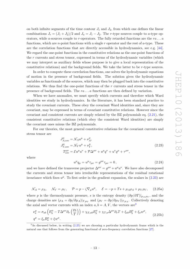
NA = ρA, NV = ρV , P = p− ζ∇µuµ, E = −p+ Ts+ µAρA + µV ρV , (2.25a)
where p is the thermodynamic pressure, s is the entropy density (∂p/∂T )|µA,µV , and the
charge densities are (ρA = ∂p/∂µA)|T,µV and (ρV = ∂p/∂µV )|T,µA . Collectively denoting
the axial and vector currents with an index a, b = A, V , the vectors are3
νµa = σab
(Eµb − T∆µν∂ν
(µbT
))+ χE,abE
µb + χT,a∆
µν∂νT + ξabBµb + ξaw
µ,
qµ = ξaBµa + ξwµ.
(2.25b)
3As discussed below, in writing (2.25) we are choosing a particular hydrodynamic frame which is the
natural one that follows from the generating functional of zero-frequency correlation functions [27].
– 13 –
JHEP10(2013)186
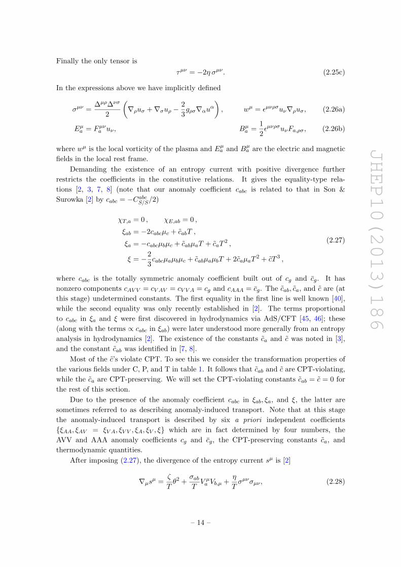
Finally the only tensor is
τµν = −2η σµν . (2.25c)
In the expressions above we have implicitly defined
σµν =∆µρ∆νσ
2
(∇ρuσ +∇σuρ −
2
3gρσ∇αuα
), wµ = εµνρσuν∇ρuσ, (2.26a)
Eµa = Fµνa uν , Bµa =
1
2εµνρσuνFa,ρσ, (2.26b)
where wµ is the local vorticity of the plasma and Eµa and Bµa are the electric and magnetic
fields in the local rest frame.
Demanding the existence of an entropy current with positive divergence further
restricts the coefficients in the constitutive relations. It gives the equality-type rela-
tions [2, 3, 7, 8] (note that our anomaly coefficient cabc is related to that in Son &
Surowka [2] by cabc = −CabcS/S/2)
χT,a = 0 , χE,ab = 0 ,
ξab = −2cabcµc + cabT ,
ξa = −cabcµbµc + cabµaT + caT2 ,
ξ = −2
3cabcµaµbµc + cabµaµbT + 2caµaT
2 + cT 3 ,
(2.27)
where cabc is the totally symmetric anomaly coefficient built out of cg and cg. It has
nonzero components cAV V = cV AV = cV V A = cg and cAAA = cg. The cab, ca, and c are (at
this stage) undetermined constants. The first equality in the first line is well known [40],
while the second equality was only recently established in [2]. The terms proportional
to cabc in ξa and ξ were first discovered in hydrodynamics via AdS/CFT [45, 46]; these
(along with the terms ∝ cabc in ξab) were later understood more generally from an entropy
analysis in hydrodynamics [2]. The existence of the constants ca and c was noted in [3],
and the constant cab was identified in [7, 8].
Most of the c’s violate CPT. To see this we consider the transformation properties of
the various fields under C, P, and T in table 1. It follows that cab and c are CPT-violating,
while the ca are CPT-preserving. We will set the CPT-violating constants cab = c = 0 for
the rest of this section.
Due to the presence of the anomaly coefficient cabc in ξab, ξa, and ξ, the latter are
sometimes referred to as describing anomaly-induced transport. Note that at this stage
the anomaly-induced transport is described by six a priori independent coefficients
ξAA, ξAV = ξV A, ξV V , ξA, ξV , ξ which are in fact determined by four numbers, the
AVV and AAA anomaly coefficients cg and cg, the CPT-preserving constants ca, and
thermodynamic quantities.
After imposing (2.27), the divergence of the entropy current sµ is [2]
∇µsµ =ζ
Tθ2 +
σabTV µa Vb,µ +
η
Tσµνσµν , (2.28)
– 14 –
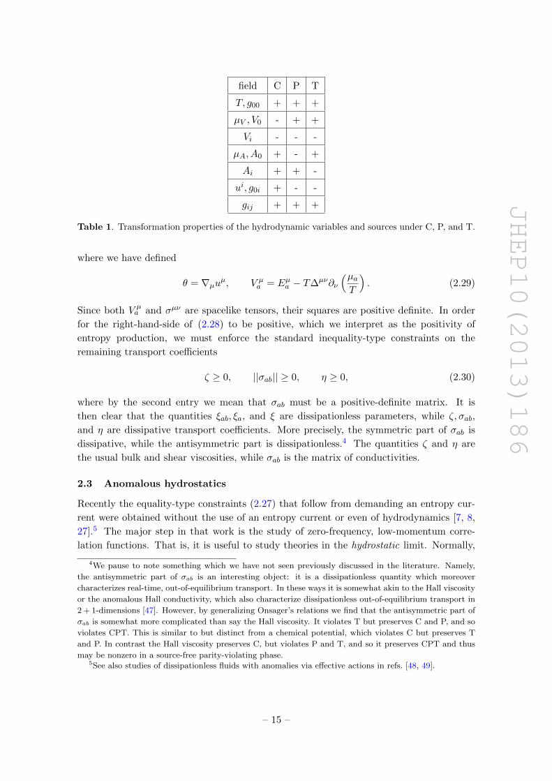
JHEP10(2013)186
field C P T
T, g00 + + +
µV , V0 - + +
Vi - - -
µA, A0 + - +
Ai + + -
ui, g0i + - -
gij + + +
Table 1. Transformation properties of the hydrodynamic variables and sources under C, P, and T.
where we have defined
θ = ∇µuµ, V µa = Eµa − T∆µν∂ν
(µaT
). (2.29)
Since both V µa and σµν are spacelike tensors, their squares are positive definite. In order
for the right-hand-side of (2.28) to be positive, which we interpret as the positivity of
entropy production, we must enforce the standard inequality-type constraints on the
remaining transport coefficients
ζ ≥ 0, ||σab|| ≥ 0, η ≥ 0, (2.30)
where by the second entry we mean that σab must be a positive-definite matrix. It is
then clear that the quantities ξab, ξa, and ξ are dissipationless parameters, while ζ, σab,
and η are dissipative transport coefficients. More precisely, the symmetric part of σab is
dissipative, while the antisymmetric part is dissipationless.4 The quantities ζ and η are
the usual bulk and shear viscosities, while σab is the matrix of conductivities.
2.3 Anomalous hydrostatics
Recently the equality-type constraints (2.27) that follow from demanding an entropy cur-
rent were obtained without the use of an entropy current or even of hydrodynamics [7, 8,
27].5 The major step in that work is the study of zero-frequency, low-momentum corre-
lation functions. That is, it is useful to study theories in the hydrostatic limit. Normally,
4We pause to note something which we have not seen previously discussed in the literature. Namely,
the antisymmetric part of σab is an interesting object: it is a dissipationless quantity which moreover
characterizes real-time, out-of-equilibrium transport. In these ways it is somewhat akin to the Hall viscosity
or the anomalous Hall conductivity, which also characterize dissipationless out-of-equilibrium transport in
2 + 1-dimensions [47]. However, by generalizing Onsager’s relations we find that the antisymmetric part of
σab is somewhat more complicated than say the Hall viscosity. It violates T but preserves C and P, and so
violates CPT. This is similar to but distinct from a chemical potential, which violates C but preserves T
and P. In contrast the Hall viscosity preserves C, but violates P and T, and so it preserves CPT and thus
may be nonzero in a source-free parity-violating phase.5See also studies of dissipationless fluids with anomalies via effective actions in refs. [48, 49].
– 15 –
JHEP10(2013)186
nonzero temperature leads to a finite static correlation length and thus screening.6 That is,
static correlation functions of all operators fall off exponentially at long distance, which in
momentum space corresponds to the statement that zero-frequency functions are analytic
at zero momentum. It then follows that the generating functional of zero-frequency corre-
lation functions Whydrostatic may be written as a local functional in a derivative expansion,
Whydrostatic =∑n
Wn +Wanom .
We collectively notate the contributions to this functional with n derivatives as Wn,
where the Wn’s are invariant under all symmetries and Wanom reproduces the anomalous
variation. This expansion will of course only have at best a finite radius of convergence, up
to momenta corresponding to the inverse screening length. The resulting object is propor-
tional to the Euclidean generating functional evaluated for stationary background fields.
Theories which are gauge and diffeomorphism invariant will have a generating func-
tional involving local gauge and diffeomorphism-invariant scalars built out of the back-
ground fields. In addition to the background fields themselves, those scalars may depend
on quantities that involve a timelike vector field Kµ which covariantly defines what we
mean by time. More precisely, we consider backgrounds where the Lie derivative of K,
LK , annihilates the background gauge fields and metric. As a result K generates a time-
like isometry. We define time through the integral curves of K. Since the background is
time-independent, we may define a thermal partition function in the usual way after Eu-
clideanizing time and compactifying the resulting time circle with coordinate periodicity β.
There are then additional gauge-invariant tensors involving K. We define the
suggestively named
T−1 =
∫ β
0dτ√−K2(τ), uµ =
Kµ
√−K2
, µa = T
∫Aa, (2.31)
where the holonomy in the last expression is around the time circle and τ is an affine
parameter along the time circle. These quantities are independent but their derivatives
are not. These satisfy some differential interrelations which follow from the fact that K
generates a symmetry of the background,
∇µuν = −uµaν + ωµν , (∇µ + aµ)T = 0, (∇µ + aµ)µa = Ea,µ, (2.32)
where we have defined local acceleration and local vorticity
aµ = uν∇νuµ, ωµν =∆µρ∆νσ
2(∇ρuσ −∇σuρ). (2.33)
Note that the tensor structures which correspond to dissipation — the shear tensor σµν ,
expansion ∇µuµ, and the vector combinations (∇µ + aµ)T and Eµa − T∆µν∂ν(µaT
)— all
vanish, corresponding to the fact that we are indeed studying the theory in a stationary
6The notable exceptions are theories in a superfluid phase, which have a propagating Goldstone mode,
theories with dynamical U(1) gauge fields like those we study later in this work, and theories tuned to a
critical point.
– 16 –
JHEP10(2013)186
equilibrium. The most general gauge-invariant tensor is built out of these quantities, the
curvatures FA,µν and FV,µν , the Riemann tensor Rµνρσ, and covariant derivatives thereof.
By varying Wn with respect to sources we obtain the one-point functions of operators
as a functional of background fields with terms that include n derivatives. However, since
we are studying real-time finite temperature field theory we should be careful to specify the
correlation functions that are computed from Wn, whether ra . . . a functions or otherwise.
Fortunately, it turns out that this caution is unnecessary for the following reason. The
correlation functions computed from Wn lead to zero-frequency functions upon Fourier
transform. Any such zero-frequency function, whether the fully retarded ra . . . a functions
or the fully symmetrized r . . . r functions, is proportional to the corresponding Euclidean
zero-frequency function [50].
As a result we may regard the variations of Wn as giving ra . . . a functions at zero
frequency with n factors of momentum. These same correlation functions are computed
in hydrodynamics and so we may match the two, thereby relating parameters of Wn to
nth order hydrodynamic coefficients. From the perspective of hydrodynamics, the resulting
one-point functions express the constitutive relations in a specific hydrodynamic frame
(a definition of hydrodynamic variables such as T , uµ, see e.g. [51]). This frame has been
termed the thermodynamic frame [27], and exhibits several important properties. One is the
fact that coefficients that appear in Wn encode thermodynamic (or hydrostatic) response
coefficients in the constitutive relations with n (and only n) derivatives [27]. Since we study
the response of the source-free thermal state to long-wavelength background sources, this
implies a direct matching between the derivative expansion of the generating functional to
the derivative expansion of hydrodynamics. Furthermore, the anomaly-induced response
described by Whydrostatic (see Wanom below in (2.36)), which includes terms from the abelian
anomaly with one derivative and the mixed anomaly with three derivatives, matches terms
in the constitutive relations with exactly one [7, 52] and three derivatives [4]. In other
hydrodynamic frames, e.g. the Landau frame, the parameters appearing in Wn will appear
at nth and generally all higher orders in the gradient expansion [53, 54]. We implicitly
work in the thermodynamic frame for the rest of this subsection.
At zeroth order in derivatives, the only gauge-invariant scalars are the local temper-
ature T and chemical potentials µa, and so the most general gauge-invariant scalar is an
arbitrary function of these which we call p(T, µa). At first order in derivatives, it turns out
that the the only gauge-invariant scalars are terms which are analogous to Chern-Simons
terms in that their gauge and coordinate variation is a total derivative. Only keeping the
CPT-preserving one-derivative terms, we have
W0 =
∫d4x√−g p(T, µa), W1 =
∫d4x√−g (cAAµ + cV Vµ)T 2wµ, (2.34)
where wµ is constructed from derivatives of uµ in the same way as in (2.26) and the caare suggestively named constants. Remarkably, if we pick a coordinate and gauge choice
– 17 –
JHEP10(2013)186
in which K = ∂t and the background fields are explicitly time-independent,7
A = A0(x)(dt+ ai(x)dxi) + Ai(x)dxi,
V = V0(x)(dt+ aidxi) + Vi(x)dxi,
g = −e2s(x)(dt+ aidxi)2 + gij(x)dxidxj ,
(2.35)
then we can write down a local functional whose gauge and coordinate variation gives
the correct anomalous variation of Whydrostatic. For the definition of consistent currents
in (2.17), that functional is [7]
Wanom =−2
∫(dt) ∧ A ∧
[cgV0
(dV +
V0
2da
)+cg3A0
(dA+
A0
2da
)]−cs
∫A ∧ V ∧ FV +Wgrav,
(2.36)
where (dt) = −iβ as we mentioned in the Introduction, and Wgrav is a complicated
functional with three derivatives. Its precise expression is given in [4] and is (thankfully)
unimportant for this work. Before going on, we note that the functional Wanom reproduces
the correct anomalous variation independently of the gradient expansion and so goes beyond
the hydrostatic limit. It is an exact part of the zero-frequency generating functional.
This gauge and coordinate choice also manifests that the terms in W1 (2.34) which
involve the ca are rather special. They may be written as Chern-Simons forms on the
spatial slice [7],
W1 = − 1
β2
∫(dt) ∧ (cV V + cAA) ∧ da , (2.37)
where the factors of β are required by dimensional analysis. The reader may note
that there are other Chern-Simons terms we may have added to W1, proportional to
A ∧ dA, V ∧ dV , A ∧ dV , and a ∧ da. However all of these terms violate four-dimensional
CPT, and we will set them to zero in this section. Despite the fact that these terms
violate CPT, we note that they are still related to the entropy current analysis. Indeed
a short calculation shows that these Chern-Simons terms correspond precisely to the
CPT-violating coefficients cab and c in (2.27).
The covariant currents which follow from the variation of W0 +W1 +Wanom by (2.20)
are precisely those (2.23) we discussed earlier in hydrodynamics. They have expressions
of the form (2.25) after setting the dissipative tensor structures to vanish, i.e. taking
θ, V µa , (∇µ+aµ)T, σµν → 0 (see (2.29) for the definitions of θ and V µ
a ). Most importantly,
the remaining coefficients in (2.25) are related to the parameters in W0 +W1 +Wanom by
the same equality-type relations (2.27) that originally came from demanding the existence
of an entropy current. More simply, the hydrostatic generating functional independently
derives the equality-type relations, including those involving the anomalies, without
reference to hydrodynamics.
We can characterize the anomaly-induced response coefficients ξab, ξa, and ξ via Kubo
formulae. That is, by computing the appropriate correlation functions in hydrodynamics
or by varying the generating functional, we may evaluate ξab, ξa, ξ in a given theory. One
7Note that we study theories subjected to real background fields in Lorentzian signature. The corre-
sponding Euclideanized background fields are necessarily complex.
– 18 –
JHEP10(2013)186
useful set of Kubo formulae for these coefficients is given by simply varying the generating
functional twice to obtain zero-frequency two-point functions, that is by studying the two-
point functions of the consistent currents.
However, the usual two-point functions in the literature involve the variation of a co-
variant current with respect to background fields, which gives the mixed two-point function
of a covariant current with a consistent one. For instance we have
〈J ia,cov(k)J jb (−k)〉 =1√−g
δ〈J ia,cov(k)〉δAb,j(k)
, (2.38)
Computing two-point functions of this type in hydrostatics leads to Kubo formulae for the
chiral conductivities (see also [6])
limk→0
iεijkkk2k2
〈J ia,cov(k)J jb (−k)〉 = ξab,
limk→0
iεijkkk2k2
〈J ia,cov(k)T 0j(−k)〉 = ξa,
limk→0
iεijkkk2k2
〈T 0icov(k)J j(−k)〉 = ξa,
limk→0
iεijkkk2k2
〈T 0icov(k)T 0j(−k)〉 = ξ.
(2.39)
The two-point functions of consistent currents are slightly different, owing to the variation
of the BZ polynomials. We have instead
limk→0
iεijkkk2k2
〈J ia(k)J jb (−k)〉 = ξab + δξab,
limk→0
iεijkkk2k2
〈J ia(k)T 0j(−k)〉 = ξa,
limk→0
iεijkkk2k2
〈T 0i(k)T 0j(−k)〉 = ξ,
(2.40)
where δξab is the symmetric matrix
δξab =
(2cg3 A0 csV0
csV0 2(cg − cs)A0
), (2.41)
and we take the ordering to be a, b = A, V . Note that the two-point function
〈T 0i(k)J ja(−k)〉 is related to 〈J ia(k)T 0j(−k)〉 by i ↔ j, k → −k. The quantities V0 and
A0 are the background values of the time-components of Vµ and Aµ, which in a flat-space
equilibrium are related to µV and µA by V0 = µV and A0 = µA.
We can summarize the anomaly-induced response in terms of a 3 × 3 matrix of zero-
frequency ‘conductivities’, characterized by the correlators〈J iV (k)J jV (−k)〉 〈J iV (k)J jA(−k)〉 〈J iV (k)T 0j(−k)〉〈J iA(k)J jV (−k)〉 〈J iA(k)J jA(−k)〉 〈J iA(k)T 0j(−k)〉〈T 0i(k)J jV (−k)〉 〈T 0i(k)J jA(−k)〉 〈T 0i(k)T 0j(−k)〉
. (2.42)
– 19 –
JHEP10(2013)186
The O(k) terms form a symmetric matrix with six coefficients, which determine the six
response parameters ξAA, ξAV = ξV A, ξV V , ξA, ξV , ξ.As discussed earlier, the relations (2.27) link the response parameters to anomaly coef-
ficients. However, there are also two CPT-preserving coefficients, cV and cA which appear
unconstrained. Recently, calculations at weak [55] and strong [56] coupling indicated that
the parameters ca were in fact proportional to the mixed flavor-gravitational anomaly co-
efficients. In the present instance, the relation is
cV = 0, cA = −8π2cm . (2.43)
It has proven surprisingly difficult to understand the origin of these relations and the
circumstances under which they hold. Both cA and cm appear in the zero-frequency two-
point function of the axial current with the stress tensor, and substituting (2.43) we have
〈J iA(k)T 0j(−k)〉 = · · ·+ 8π2cmT2O(k) + cmO(k3). (2.44)
With the identification (2.43), cm apparently contributes to both the O(k) and O(k3)
parts of the zero-frequency functions respectively, and there is a relative transcendental
factor of ∼ π2 between them. The methods discussed thus far — demanding the existence
of an entropy current or studying the hydrostatic generating functional — treat each order
in momenta independently and furthermore lead to algebraic, rather than transcendental,
relations between response coefficients. Indeed, the two terms involving cm in (2.44) are
comparable at a momentum scale k ∼ 2πT , which is outside of the hydrostatic regime.
This suggests that a proof of (2.43) must go beyond the hydrodynamic limit.
There are currently two independent proofs of (2.43). One [4] involves studying the Eu-
clidean theory on a conical geometry which interpolates between the thermal cylinder and
the vacuum. This generalizes the Cardy formula [57, 58] in two-dimensional conformal field
theory (CFT), which relates the pressure of a 2d CFT to its central charge. The second [21]
involves a direct integration of a Weyl fermion in the Matsubara formalism. The resulting
tower of Dirac Matsubara modes in the dimensionally reduced spatial theory provides a one-
loop shift of the Chern-Simons terms, and again leads to (2.43). We refer the reader to these
references for further details of the caveats and assumptions relevant for each derivation.8
From this discussion it is clear that when applied to Standard Model physics, the
relation (2.43) as well as all of the anomaly-induced response in (2.27) may be modified. The
reason is that all of the results above were obtained assuming that the anomalies are shared
between global symmetries. As a result, when taking one of the U(1) symmetries to be
weakly gauged all of the anomaly-induced response may in principle be subject to radiative
corrections. We undertake a systematic study of these corrections in the rest of this work.
8Curiously, (2.43) seems to hold in theories which do not contain fields of spin greater than 1, which are
sensitive to topology. For instance, the partition function of a theory of free gravitinos on R2,∗ does not
agree with the partition function of the same theory on R2 due to the Killing spinors broken by deleting
the origin [59]. Correspondingly, the relation (2.43) does not hold for chiral gravitinos [60].
– 20 –
JHEP10(2013)186
3 Weak gauging and dynamical photons
The discussion in section 2 focused on theories with global U(1)V and U(1)A symmetries,
which are broken by AV V , AAA, and ATT anomalies in the presence of non-dynamical
background fields Vµ and Aµ, and gµν . When Vµ is dynamical, the generating functional
and the hydrodynamic description need to be modified. In this and the following section
we discuss the effects of the dynamical photon field Vµ, under the assumption of weak
gauging, i.e. a perturbatively small gauge coupling.
3.1 Anomalous conservation laws
When Vµ is the dynamical field, the full generating functional W [V,A, g] of section 2.1
becomes the effective action for the photon, so that we define
Z[Jext, A, g] =
∫[dVµ] exp
[iW [V,A, g] + i
∫d4x√−g VµJµext
]. (3.1)
There is now a functional integral over the photon field which we couple to an external
conserved current, ∇µJµext = 0. We will use Jµext to compute correlation functions of
Vµ as well as to ensure that the equilibrium at nonzero µV is stable [61]. When U(1)Vis dynamical, the generating functional W [V,A, g] must ensure that the corresponding
consistent current JµV of section 2.1 is conserved, ∇µJµV = 0. This amounts to choosing
cs = 0 in eq. (2.17), so that W [V,A, g] is gauge-invariant under U(1)V . The generating
functional of the theory with a dynamical Vµ is given in the usual way by
W [Jext, A, g] = −i lnZ[Jext, A, g] . (3.2)
The one-point functions of the energy-momentum tensor, the axial current, and the photon
field in the presence of external sources may be defined by the usual variational procedure,
T µν ≡ 2√−gδW
δgµν, J µA ≡
1√−gδW
δAµ, Vµ ≡
1√−gδW
δJµext
. (3.3)
As a result of conservation of Jµext, physical quantities are invariant under Vµ → Vµ+∂µΛ(x),
for an arbitrary Λ(x). We can also write
T µν = 〈Tµν〉+ gµν〈VλJλext〉 , J µA = 〈JµA〉 , Vµ = 〈Vµ〉 , (3.4)
where Tµν and JµA are the stress tensor and axial current that follow from variation of W
as in (2.2), and the brackets denote averaging over the photon field configurations. The
anomalous conservation laws for the consistent stress tensor and current T µν and J µA are
similar to (2.14),
∇µJ µA =1
4εµνρσ
[cg〈FV,µνFV,ρσ〉+
cg3FA,µνFA,ρσ + cmR
αβµνR
βαρσ
],
∇νT µν = FµνA JA,ν −1
4Aµενρστ
[cg〈FV,νρFV,στ 〉+
cg3FA,νρFA,στ + cmR
αβνρR
βαστ
].
Compared to (2.14), there is no FµνV JV,ν term in the right-hand side, as it is already
contained in the divergence of the energy-momentum tensor T µν .
– 21 –
JHEP10(2013)186
3.2 Anomalous (magneto-)hydrodynamics
The main modification to hydrodynamics is that Vµ now needs to be included as one of the
hydrodynamic variables. This is based on the familiar statement that static U(1) magnetic
fields are not screened, hence for excitations with sufficiently low frequency, one adds the
magnetic field to the set of hydrodynamic variables. This leads to magneto-hydrodynamics,
or MHD, a description where magnetic fields are treated classically, on par with other
hydrodynamic variables such as T and uµ, see e.g. [62] (anomalies in MHD have also
been discussed in [3]). Taking quantum fluctuations of Vµ into account for low-frequency
collective excitations requires a treatment that goes beyond classical hydrodynamics.
If the gauge coupling of U(1)V is sufficiently small, we may consider classical
configurations of the photon field, which we call vµ, which solve the classical equations of
motion, extremizing the exponent in (3.1),
Jµv + Jµext = 0 . (3.5)
Here Jµv = 1√−g
δWδVµ
∣∣V=v
is the conserved current obtained by the variation of W [V,A, g].
The hydrodynamic variables are thus T , µV , µA, uµ, and vµ, where µV and µA are defined
so as to match the Euclidean temporal holonomies of Vµ and Aµ in equilibrium. As
noted earlier, µA as defined is not conjugate to a conserved charge when Vµ is dynamical.
However, the non-conservation of JµA is gradient-suppressed, and we will continue to
include µA as a hydrodynamic variable.
Eq. (3.5) should be viewed as an analogue of Maxwell’s equations, specifying the
dynamics of vµ. Note that upon solving (3.5), the current Jµv is conserved, so that
∇µJµv = 0 is not a new hydrodynamic equation. Such classical treatment neglects
photon loops, and in a slight abuse of terminology we will call this effective description
magneto-hydrodynamics, or MHD.
The other hydrodynamic equations are the anomalous conservation laws of the axial
current and the energy-momentum tensor,
∇µJµA =1
4εµνρσ
[cgFv,µνFv,ρσ +
cg3FA,µνFA,ρσ + cmR
αβµνR
βαρσ
],
∇νTµν = FµνA JA,ν −1
4Aµενρστ
[cgFv,νρFv,στ +
cg3FA,νρFA,στ + cmR
αβνρR
βαστ
].
(3.6)
where JµA and Tµν are J µA and T µν , evaluated when Vµ is treated as a classical field solv-
ing (3.5). In four spacetime dimensions, there are 9 hydrodynamic equations (3.5), (3.6),
and 10 hydrodynamic variables T , µV , µA, uµ, vµ. The U(1)V gauge freedom can be used
to eliminate the extra degree of freedom in vµ.
In the thermodynamic frame, the constitutive relations for JµA and Tµν in MHD are
exactly the same as in section 2.2, expressed in terms of T , µV , µA, uµ, vµ, Aµ and gµν .
As in section 2.2, we adopt the scaling such that the gauge fields and the metric are O(1)
in the derivative expansion, hence Fv,µν and FA,µν are O(∂), and Rµναβ is O(∂2). This
scaling does not allow us to consider a background magnetic field at zeroth order in the
derivative expansion.
– 22 –
JHEP10(2013)186
In order to find Jµv [v,A, g], one in principle needs to know W [V,A, g], which is a
complicated non-local functional. However, W [V,A, g] is the generating functional in the
theory with the global U(1)V ; hence the relation
1√−gδW
δVµ= JµV ,
can be viewed as providing an expression for 1√−g
δWδVµ
in the hydrodynamic limit, when the
right-hand side, expressed as JµV [V,A, g], is determined by the hydrodynamic equations in
the theory with global U(1)V . Thus one has to solve the hydrodynamic equations in the
theory with global U(1)V , express the current JµV in terms of Vµ, Aµ, and gµν (which all
act as sources when U(1)V is global), and use the resulting Jµv = JµV [V,A, g]V=v in (3.5)
in order to find vµ[A, g, Jext]. Once the dynamics of vµ is determined, the remaining
equations (3.6) can be used to express the hydrodynamic variables T , µV , µA, uµ in terms
of the sources, and eventually find JµA[A, g, Jext] and Tµν [A, g, Jext].
Any solution to the MHD equations (3.5), (3.6) is also a solution to the hydrodynamic
equations (2.14) in the theory with global U(1)V (obviously, Jµv + Jµext = 0 as fixed by the
dynamics of the photon field implies∇µ(Jµv +Jµext) = 0). Therefore the entropy current with
non-negative divergence in the hydrodynamic theory with global U(1)V will have a non-
negative divergence when evaluated on the solutions to MHD. This shows that an entropy
current in MHD can be taken to be exactly the same as the entropy current in the theory
with global U(1)V . It is not clear from this argument, however, whether this provides the
unique MHD entropy current. We hope to return to this question in the future.
We now turn to the question of MHD correlation functions. The prescription is almost
identical to the variational method in hydrodynamics outlined in section 2.2. Namely, the
MHD equations (3.5), (3.6) need to be solved in order to find the hydrodynamic variables
in terms of the sources Aµ, gµν , and Jµext, which upon using the constitutive relations give
vµ[A, g, Jext], JµA[A, g, Jext] and Tµν [A, g, Jext]. Varying with respect to the sources then
allows one to compute (retarded) correlation functions of JµA, Tµν , and Vµ.
The correlation functions of the vector current are more subtle, as the on-shell value of
Jµv is just −Jµext, which does not depend on the A and g sources. This implies in particular
that the correlation functions defined by varying Jµv with respect to Aν and gρσ vanish iden-
tically in MHD. However, one should keep in mind that the current JµV does not in general
coincide with the expectation value of the conserved current operator whose charge gener-
ates the U(1)V symmetry. We call the latter current operator JµV. For example, in flat-space
quantum electrodynamics 〈JµV〉 and JµV differ by a term proportional to ∂νFµνV which is iden-
tically conserved [31]. Within the hydrodynamic description with classical vµ, we will write
Jµv = 〈JµV〉 − C µ , (3.7)
where C µ is an identically conserved vector built out of hydrodynamic variables and
background sources. Setting Jµext = 0 for simplicity, so that 〈JµV〉 = C µ according to (3.5),
we parametrize C µ in the following way, to second order in derivatives,
C µ = C µ(1) + C µ
(2) + · · · (3.8)
– 23 –
JHEP10(2013)186
where
C µ(1) = ∇ν
[j0u
[µAν]]
+ εµνρσ∇ν[j0uρAσ
](3.9)
C µ(2) = ∇ν
[(j1F
µνv + j2F
µνA + j3ω
µν + j4u[µEν]
v + j5u[µE
ν]A + j6u
[µaν]
+j7u[µ∂ν]µV + j8u
[µ∂ν]µA + j9u[µ∂ν]T )
)]+ εµνρσ∇ν
[j1Fv,ρσ + j2FA,ρσ + j3ωµν + j4uρEv,σ + j5uρEA,σ + j6uµaν
+j7uρ∂σµV + j8uρ∂σµA + j9uρ∂σT]
+ (U(1)A-violating).
(3.10)
The brackets indicate antisymmetrization, T [µν] = 12(Tµν − T νµ). The vector C µ is
invariant under U(1)V , but not under U(1)A, as the latter is explicitly broken by the
anomaly. We have neglected U(1)A-violating terms at O(∂2) as one can show that they are
unimportant for our analysis later in this article. The parameters ji and ji are functions
of T, µV , µA, uµAµ, and AµA
µ. Expressing C µ in terms of the sources Aµ and gµν upon
solving the hydrodynamic equations allows one to compute correlation functions of one
JµV with multiple JµA and Tµν . These correlation functions will be given in terms of the
parameters ji and ji which need to be determined by matching to the microscopic theory.
To compute correlation functions involving more than one vector current, it may be
helpful to reformulate the classical MHD equations as tree-level perturbation theory. For
example, in order to evaluate the two-point function of JµV, one needs all tree-level diagrams
that connect two factors of C µ, expressed in terms of the tree-level propagators of the
hydrodynamic variables. The MHD described above requires a small gauge coupling for
U(1)V , and as a classical theory it neglects loop of both photons and other collective
excitations. We leave the detailed study of MHD correlation functions for future work.
3.3 Anomalous (magneto-)hydrostatics
3.3.1 The (magneto-)hydrostatic effective theory
In section 2.3 we reviewed how the hydrostatic response of a theory where the photon is
non-dynamical may be calculated directly from the generating functional Whydrostatic de-
fined on the spatial slice. In a gauge and coordinate choice where the background fields
are explicitly time-independent, Whydrostatic[V,A, g] is a local functional (unlike the full
W [V,A, g]), thanks to the finite static correlation length. When the photon is dynami-
cal, the unscreened static magnetic field will make the corresponding generating functional
W [Jext, A, g] non-local even in the static limit, making a derivative expansion of W im-
practical. Instead, a convenient static low-momentum effective description can given by a
dimensionally reduced Euclidean field theory, as in [24–26]. The effective theory describes
the Matsubara zero mode of the four-dimensional photon, below the momentum cutoff
scale Λ . T whose exact value is determined by the masses of the other fields in the mi-
croscopic theory. The cutoff is such that the zero mode of the photon is the lightest degree
of freedom. Let us now write down the action of this three-dimensional effective theory,
taking into account AAA, AV V , and ATT anomalies.
– 24 –
JHEP10(2013)186
We turn on the external sources A, g, and Jext which are time-independent, with
momenta below the cutoff. We will write the action Seff [V ;A, g] in the derivative expansion,
Seff = S(0)eff + S
(1)eff + S
(2)eff +O(∂3) , (3.11)
where S(n)eff denotes the terms in Seff with n derivatives. In principle, Seff may be obtained
by starting with the partition function (3.1), continuing to Euclidean (compact) time, inte-
grating out all of the nonzero Matsubara modes of Vµ, integrating out all spatial momenta
above the scale Λ, and then continuing the photon field back to real time. At weak U(1)Vgauge coupling, the resulting Seff will be equal to the hydrostatic generating functional
Whydrostatic of section 2.3, plus perturbative corrections that come from loops with momenta
above the cutoff. If we neglect photon loops, as in MHD, then Seff is precisely Whydrostatic.
The action Seff must be both U(1)V and diffeomorphism-invariant, but it need not be
U(1)A-invariant. The U(1)A-violating terms have two distinct origins: (i.) there are the
anomalous U(1)A-violating terms in Whydrostatic given by eq. (2.36), and (ii.) there are
terms which come from integrating out higher Matsubara modes and momenta above the
cutoff. The latter are perturbatively suppressed under our weak gauging assumption, and
we will explicitly account for this in parametrizing the operator coefficients in Seff .
In terms of the time-independent fields (2.35), the zero-derivative piece is
S(0)eff =
∫(dt) d3x es
√g (p(T, µV , µA) + δp+ VµJ
µext) (3.12)
where p is the pressure of the theory with Vµ non-dynamical, and the second term
δp = δp(T, µV , µA, A2) arises from integrating out the photon field with momenta above
the cutoff. It depends on
T = e−sβ−1 , µV = e−sV0 , µA = e−sA0 , A2 = gijAiAj . (3.13)
After matching the anomaly-induced terms, which we can separate out according to our
weak-gauging assumption, the functional form of the one-derivative effective action is
S(1)eff = Wanom +W1 + . . . ,
where Wanom and W1 are given by (2.36) and (2.37), respectively. Specifically,
S(1)eff =−
∫(dt) d3x ε ijk
[(2cgV0+
cAVβ−δfAV
)Ai∂j Vk+
(2cg3A0+
cAA2β−δfAA
)Ai∂jAk
+
(cgV
20 +
cg3A2
0 +cAβ2− δfAa
)Ai∂jak (3.14)
− cV V2β
Vi∂j Vk +cVβVi∂jak −
c
2β3ai∂jak
]+ δS
(1)eff ,
where cAA, cAV , and cA are constants which respect U(1)A. The coefficients cV V , cV , and
c are constants, due to U(1)V and U(1)KK gauge invariance. Since they are Chern-Simons
couplings in the three-dimensional theory, they only receive corrections at one-loop order
– 25 –
JHEP10(2013)186
from charged fields [30]. Indeed, the diagrammatic analysis of Coleman and Hill [30] indi-
cates, under fairly general assumptions, that radiative corrections to abelian Chern-Simons
coefficients arise only from fermions at one-loop order. There are no fermions in the
effective theory, and thus the constant coefficients should be equal to their values before
gauging U(1)V . In particular, cV = 0 and, due to the ATT anomaly, cA = −8π2cm [4, 21].
Nonperturbative arguments against higher loop corrections to the c’s can also be made by
exploiting analyticity of the Wilsonian effective action [63]. As mentioned in section 1, we
retain the CPT-violating constants to facilitate contact with physics at nonzero µ5.
The functions δf depend on T, µV , µA, and A2 and come from integrating out non-zero
Matsubara modes of all the fields in the theory, plus the high momentum component of
the photon zero modes. The remaining U(1)A-violating corrections δS(1)eff are also induced
perturbatively,
δS(1)eff =
∫(dt) d3x es
√g[(δfdA g
ij + δfAAdA AiAj)∇iAj
+ gij(δfAV Ai∂jV0 + δfAA Ai∂jA0 + δfAs Ai∂js
)].
(3.15)
The full expression for the two-derivative part S(2)eff is rather long. For the purpose of
computing the leading perturbative corrections to two-point functions of spatial currents
and the momentum density, the only relevant terms in S(2)eff are U(1)A-invariant terms
which do not involve gradients of s, A0, and gij . The U(1)A-violating terms may be shown
to contribute to the two-point functions at higher order in the U(1)V gauge coupling
than we consider (in QED they contribute at order e4 and higher). We summarize the
scalars and pseudoscalars which appear in S(2)eff and are relevant for us in table 2. For
completeness, the second-order U(1)A-invariant terms which are irrelevant for us are
scalars: R , (∂s)2 , fijfij , (∂A0)2 , fijF
ijA , FA,ijF
ijA , ∂is∂
iA0 , ∂is∂iV0 , ∂iA0∂
iV0 ,
pseudoscalars: εijk∂is∂jak, εijk∂is∂jAk, ε
ijk∂is∂j Vk, εijk∂iA0∂jak, ε
ijk∂iA0∂jAk, εijk∂iA0∂j Vk ,
where R is the Ricci curvature scalar constructed from the spatial metric g, fij = ∂iaj−∂jai,and FV and FA are the field strengths constructed from Vi and Ai. The epsilon tensor on
the spatial slice is εijk = ε ijk/√g, with ε 123 = 1. We then have
S(2)eff =
∫(dt) d3x es
√g
[4∑i=1
aisi +
3∑i=1
aisi
]+ (irrelevant terms) , (3.16)
where the ai’s and ai’s are functions of T, µV , and µA, and the scalars si and pseudoscalars
si are defined in table 2. As we will see, to accurately compute the chiral conductivities to
low order in perturbation theory, we also require a single parity-violating term with three
derivatives. This term is singled out relative to the other two- and three-derivative terms
in that it contributes to the spatial photon propagator at low order in momentum. It is
S(3)eff =
∫(dt) d3x es
√g a4 ε
ijk(FV )ij∇l(FV ) lk + (irrelevant terms) . (3.17)
We may use the effective theory (3.11) to calculate in the hydrostatic limit the correlation
– 26 –
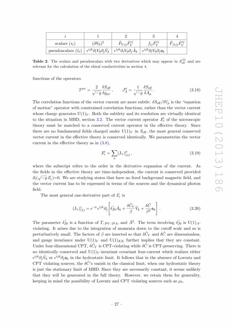
JHEP10(2013)186
i 1 2 3 4
scalars (si) (∂V0)2 FV,ijFijV fijF
ijV FA,ijF
ijV
pseudoscalars (si) εijk∂iV0∂j Vk εijk∂iV0∂jAk εijk∂iV0∂jak
Table 2. The scalars and pseudoscalars with two derivatives which may appear in S(2)eff and are
relevant for the calculation of the chiral conductivities in section 4.
functions of the operators
Tµν =2√−g
δSeff
δgµν, JµA =
1√−gδSeff
δAµ. (3.18)
The correlation functions of the vector current are more subtle: δSeff/δVµ is the “equation
of motion” operator with constrained correlation functions, rather than the vector current
whose charge generates U(1)V . Both the subtlety and its resolution are virtually identical
to the situation in MHD, section 3.2. The vector current operator JµV of the microscopic
theory must be matched to a conserved current operator in the effective theory. Since
there are no fundamental fields charged under U(1)V in Seff , the most general conserved
vector current in the effective theory is conserved identically. We parameterize the vector
current in the effective theory as in (3.8),
JµV =∑n
(JV)µ(n) , (3.19)
where the subscript refers to the order in the derivative expansion of the current. As
the fields in the effective theory are time-independent, the current is conserved provided
∂i(√−g JiV)=0. We are studying states that have no fixed background magnetic field, and
the vector current has to be expressed in terms of the sources and the dynamical photon
field.
The most general one-derivative part of JiV is
(JV)i(1) = e−s εijk∂j
[δj0Ak +
δCVβ
Vk +δC
β2ak
]. (3.20)
The parameter δj0 is a function of T, µV , µA, and A2. The term involving δj0 is U(1)A-
violating. It arises due to the integration of momenta down to the cutoff scale and so is
perturbatively small. The factors of β are inserted so that δCV and δC are dimensionless,
and gauge invariance under U(1)V and U(1)KK further implies that they are constant.
Under four-dimensional CPT, δCV is CPT-violating while δC is CPT-preserving. There is
no identically conserved and U(1)V -invariant covariant four-current which realizes either
εijk∂j Vk or εijk∂jak in the hydrostatic limit. It follows that in the absence of Lorentz and
CPT violating sources, the δC’s vanish in the classical limit, when our hydrostatic theory
is just the stationary limit of MHD. Since they are necessarily constant, it seems unlikely
that they will be generated in the full theory. However, we retain them for generality,
keeping in mind the possibility of Lorentz and CPT violating sources such as µ5.
– 27 –
JHEP10(2013)186
The most general two-derivative piece of JiV is
(JV)i(2) =1√−g∂j
[√−g (j0F ijV + j1FijA + j2f
ij)]
+ e−s εijk∂j[j1∂kV0 + j2∂kA0 + j3∂ks
]+ (U(1)A-violating) , (3.21)
where ji and ji are functions of T, µV , and µA. The U(1)A-violating terms will contribute
to two-point functions of spatial currents beyond the leading order in perturbation theory.
Using the expressions (3.18) and (3.19) for the currents along with the photon propagators,
hydrostatic correlation functions may be computed by the usual method of diagrammatic
perturbation theory.
The effective action simplifies if we work in flat space at constant T and µV , and the
only external sources are the constant µA = A0 and J0ext. To third order in derivatives,
Seff =
∫(dt) d3x
[p(V0) +
cV V2β2
εijkVi∂j Vk + a1(V0)(∂V0)2 + a2(V0)F 2V + a1(V0)εijk∂iV0∂j Vk
+a4(V0)εijkFij ∂l(FV ) lk
]+O(∂4) . (3.22)
The effective pressure p ≡ p+ δp+ V0J0ext has a local minimum at V0 = V0 which must be
identified as V0 = µV . Around the minimum,
p(V0) = p+1
2p ′′δV 2
0 + . . . , ai(V0) = ai + a′i δV0 + . . . , ai(V0) = ai + a′i δV0 + . . . ,
(3.23)
where δV0 = V0−V0, and the prime indicates a derivative evaluated at V0. From (3.22) we
see that, ignoring the higher-derivative terms, the tree-level photon propagator is
〈δV0(k) δV0(−k)〉 = − 1 +O(k2)
2a1k2 + p ′′,
〈Vi(k)Vj(−k)〉 =i(cV V T + 2a4k
2)εijkkk + 4a2δijk2 +O(k4)
k2(c2V V T
2 − 4(4a22 − a4cV V T )k2)
,
(3.24)
where we have chosen Feynman gauge, and 〈δV0(k) Vi(−k)〉 = 0. The temporal photon has
a mass m2 = p ′′/2a1, interpreted as electric screening. Without the CPT-violating con-
stant cV V the spatial photon has no mass, which is interpreted as the absence of magnetic
screening. The Chern-Simons term in the effective action generates magnetic screening
when cV V T > 4a22/a4, and magnetic anti-screening when cV V T < 4a2
2/a4. In the pertur-
bative regime, we expect that the contribution a4 is subleading compared to a22, leading to
anti-screening [64, 65]. Recall that turning on the constant axial chemical potential µ5 (as
distinct from µA) will generate a contribution to cV V . In the full theory the anti-screening
visible in the spatial effective theory will likely lead to an instability (see e.g. the recent
discussion in [66]). We comment further on magnetic anti-screening in section 5.
3.3.2 The thermal effective action and chiral conductivities
In order to directly encode the retarded correlators, and thus the Euclidean Kubo formulae,
it is useful to consider the formal result of integrating over the remaining Matsubara zero-
modes of the photon. The effective theory Seff then leads to the generating functional
– 28 –
JHEP10(2013)186
W [Jext, A, g] in eq. (3.2) where the sources are time-independent and slowly varying. The
1PI effective action Γ[V, A, g] (that we will refer to here as the “thermal” effective action)
is related to the generating functional by a functional Legendre transform,
Γ[V, A, g] = W [Jext[V, A, g], A, g]−∫d4x√−g VµJµext[V, A, g] , (3.25)
where Vµ is now the expectation value and we solve
1√−gδW [Jext, A, g]
δJµext
= Vµ , or1√−g
δΓ[V, A, g]
δVµ= −Jµext (3.26)
for V[Jext, A, g], or equivalently for Jext[V, A, g]. Since we are only Legendre transforming
in the Jext,V variables and not in the other sources, Γ is the 1PI effective action in the
presence of fixed background Aµ and gµν .
In a zero-temperature theory with a mass gap mgap and slowly varying sources (with
gradients λ longer than the inverse gap, λmgap 1), both the generating functional
and effective action may be expressed locally in a derivative expansion. The derivative
expansion effectively accounts for the response of the vacuum to background fields,
neglecting non-localities over the scale of the inverse gap, so that the small expansion
parameter is ∼ 1/λmgap. In a theory with massless fields, both W and Γ are generically
nonlocal, reflecting the infinite correlation length.
Similar statements hold for thermal field theories subjected to time-independent
background fields. At momenta and Euclidean energies well below the temperature, the
theory dynamically dimensionally reduces on the thermal circle to give a three-dimensional
effective theory in which the temperature dependence of the full theory is fully encoded
in the mass and coupling parameters. The inverse static screening length plays the role
of a mass gap. So a thermal field theory with finite static screening length will possess a
hydrostatic generating functional which may be expressed locally in a derivative expansion
as argued in [7, 27]. The hydrostatic W effectively describes the response of the flat space
thermal state to background fields.
When the static screening length is infinite, both W and Γ will generically be
nonlocal. When the magnetic photon is massless, the derivative couplings enforced by
gauge invariance soften the infrared behaviour. The three-dimensional gauge field Vimay be dualized to a compact massless scalar, which crucially as a consequence of gauge
invariance is derivatively coupled to itself and to the massive V0.9 Such a theory should
not possess infrared divergences, and so we expect that Γ (though not W ) may in this case
be written locally in a derivative expansion. This expansion can be at best asymptotic as
it was for the hydrostatic generating functional.
Since the thermal effective action is local, we can parameterize it to low order in
derivatives in terms of the photon expectation value Vµ and the sources Aµ and gµν .
By the symmetries of the problem, we must impose U(1)V gauge invariance as well as
diffeomorphism invariance. As a result Γ has the same structure as the effective field
9The same words apply to a superfluid phase, as studied in [67]. As a result our arguments should also
apply to superfluids.
– 29 –
JHEP10(2013)186
theory action Seff , however the various coefficients that appear in it will differ from those
of the Wilsonian effective action. To first order in derivatives it is
Γ(0) =
∫(dt) d3x es
√g P , (3.27)
Γ(1) =
∫(dt) d3x ε ijk
[ϕAAAi∂jAk + ϕAV Ai∂jVk + ϕAaAi∂jak
+cV V2βVi∂jVk −
cVβ2Vi∂jak +
c
2β3ai∂jak
]+
∫(dt) d3x es
√g[(ϕdAg
ij+ϕAAdAAiAj)∇iAj+ϕAV Ai∂iV0+ϕAAA
i∂iA0+ϕAsAi∂is],
where the coefficients may be functions of µV = e−sV0, µA, T , and A2. Again, the Chern-
Simons constants cV V , cV , and c can only receive corrections at one-loop order from charged
matter, and therefore should stay the same as in (3.14). There are also some two and three
derivative terms which will be relevant when calculating the chiral conductivities. We have
Γ(2) =
∫(dt) d3x es
√g
(4∑i=1
αisi +3∑i=1
αisi
)+ (irrelevant terms) ,
Γ(3) =
∫(dt) d3x es
√g α4 ε
ijk(FV)ij∇l(FV) lk + (irrelevant terms) .
(3.28)
The one-point functions of the axial current and the energy-momentum tensor are given
by the variation of W [Jext, A, g] in (3.3). Using (3.26), they may be equivalently written
in terms of the variation of Γ[V, A, g],
〈Tµν〉 =2√−g
(δΓ
δgµν
)V,A
, 〈JµA〉 =1√−g
(δΓ
δAµ
)V,g
. (3.29)
The vector current, on the other hand, can not be derived in a similar manner because of the
constraint (3.26). Instead, the vector current JµV should be parameterized in a derivative ex-
pansion in terms of the classical photon Vµ and the sources, as in eq. (3.19). The expression
for JµV must be conserved, U(1)V gauge-invariant, and transform as a vector under coordi-
nate re-parametrization. As a result it will have the same structure as the hydrostatic ex-
pressions for JiV that we wrote down in eqs. (3.20), (3.21). To second order in derivatives it is
〈JiV〉 =e−sεijk∂j
(χ0Ak +
CVβVk +
C
β2ak
)+
1√−g∂j[√−g (χ0F
ijV + χ1F
ijA + χ2f
ij)]
+ e−sεijk∂j [χ1∂kV0 + χ2∂kA0 + χ3∂ks] + (O(∂2),U(1)A-violating terms) ,
(3.30)
where the χ’s and χ’s are functions of µV = e−sV0, µA, T , and A2, and the C’s are constants.
The two-point functions of the currents may be evaluated diagrammatically from the
effective action Seff , and expressed in terms of the parameters of Γ. The two-point functions
of the axial current and the energy-momentum tensor come from the second variation of
– 30 –
JHEP10(2013)186
W [Jext, A, g], or equivalently from the first variation of 〈JµA〉[Jext, A, g] and 〈Tµν〉[Jext, A, g],
Gµ,νAA(x) =1√−g
(δ〈JµA(x)〉δAν(0)
)Jext, g
, Gµν,σTA (x) =1√−g
(δ〈Tµν(x)〉δAσ(0)
)Jext, g
, (3.31a)
Gσ,µνAT (x) =2√−g
(δ〈JσA(x)〉δhµν(0)
)Jext, A
, Gστ,µνTT (x) =2√−g
(δ〈T στ (x)〉δhµν(0)
)Jext, A
.
After the variation, we set gµν = ηµν , Ai = 0, A0 = µA, J iext = 0, while J0ext is determined
by the neutrality constraint ∂P/∂µV = 0. If 〈JµA〉 and 〈Tµν〉 are derived from the variation
of Γ[V, A, g] as in (3.29), the correlation functions can be written in the same way (3.31a),
where now 〈JµA〉 = 〈JµA〉[V[Jext, A, g], A, g] and 〈Tµν〉 = 〈Tµν〉[V[Jext, A, g], A, g]. The
mixed correlation functions of the vector current may also be defined by the variational
procedure, given 〈JµV〉[V[Jext, A, g], A, g], such as eq. (3.30),
Gµ,νV A(x) =1√−g
(δ〈JµV(x)〉δAν(0)
)Jext, g
, Gσ,µνV T (x) =2√−g
(δ〈JσV(x)〉δhµν(0)
)Jext, A
. (3.31b)
In order to have a variational prescription for Gµ,νAV , Gµν,σTV and GµνV V , we need to
introduce a source for the vector current operator (3.19) in the effective theory,
Seff → Seff +∫√−g XµJµV. Integrating over the photon field will give rise to W [Jext, A, g,X],
and the corresponding Γ[V, A, g,X], where Vµ[Jext, A, g,X] is determined by (3.26). Similar
to (3.29) we have
〈JµV〉 =1√−g
δΓ
δXµ,
which is solved by Γ = Γ[X=0] +∫√−g Xµ〈JµV〉, as 〈JµV〉 does not depend on X. If
the vector current is linear in δV0 and Vi, the effect of X is to shift Jext by an amount
proportional to X. In this case the correlation functions of the vector current obtained
through the variation with respect to X can be built in terms of the photon propagators
obtained through the variation with respect to Jext.
To compute correlation functions in this equivalent tree-level description, we expand
the currents 〈JiV〉, 〈J iA〉, and 〈T 0i〉 to linear order in the Vµ and the background fields Aiand g0i (while keeping A0 = µA, g00 = −1, and gij = δij fixed as before), and connect
the V’s by exact photon propagators. Two-point functions receive contributions from
two types of diagrams: (i.) those with a single photon running between two operator
insertions, and (ii.) contact diagrams with no intermediate photons. In terms of the
three-dimensional fields, we have
A0 = µA , Ai = Ai +µA2g0i , s = 0 , ai = −1
2g0i , gij = δij +
1
4g0ig0j . (3.32)
To second order in derivatives, the axial and momentum currents follow from variation of
– 31 –
JHEP10(2013)186
Γ and to linear order in the photon, Ai, and g0i are given by
〈J iA〉=2∂P
∂A2
(Ai+
µA2g0i
)+εijk
[2ϕAA∂j
(Ak+
µA2g0k
)+ϕAV ∂jVk−
ϕAa2∂jg0k
]+ ϕAV ∂iδV0 + 2α4∂jF
ijV + (irrelevant two-derivative terms) ,
〈T 0i〉= 1
2Pg0i + µA〈J iA〉+ εijk
[−ϕAa∂j
(Ak +
µA2g0k
)+cVβ2∂jVk +
c
2β3∂jg0k
]− 2α3∂jF
ijV + (irrelevant two-derivative terms) ,
(3.33a)
where the omitted terms will not contribute to the two-point functions of spatial currents
to O(k). Meanwhile the vector current is
〈JiV〉 = εijk∂j
[χ0
(Ak +
µA2g0k
)+CVβVk −
C
2β2g0k
]+ ∂j(χ0F
ijV )
+ (irrelevant two-derivative terms) .
(3.33b)
The photon propagator is
〈δV0(k) δV0(−k)〉 = − 1 +O(k2)
2α1k2 + ∂2P∂µ2V
,
〈Vi(k)Vj(−k)〉 =i(cV V T + 2α4k
2)εijkkk + 4α2δijk2 +O(k4)
k2(c2V V T
2 − 4(4α22 − α4cV V T )k2)
.
(3.34)
The zero-frequency two-point functions in momentum space are
GIJ(k) = −iβ∫d3x e−ikxGIJ(x) ,
where GIJ(x) are variational correlation functions, such as (3.31a), (3.31b). The low-
momentum behavior of the two-point functions varies depending on whether the CPT-
violating constant cV V vanishes. If it vanishes, then the spatial photon is massless, the
photon propagator is ∼ δij/k2, and diagrams with a single photon contribute to the two-
point functions at low order in momentum. For example, diagrams of this type contribute
to the O(k) part of two-point functions when the spatial photon runs from an O(∂2) vertex
to a O(∂) vertex. If cV V does not vanish, then the spatial photon receives a topological mass
so that the low-momentum propagator is ∼ εijkkk/k2, in which case the single-photon dia-
grams contribute at higher order in momentum. We therefore treat these cases separately.
For cV V = 0, we find the low-momentum two-point functions to be
GijV V (k) = − C2V T
2
4α2
[δij − kikj
k2
]+ i
[CV T (4χ0α2 − CV T α4)
8α22
]εijkkk +O(k2) , (3.35a)
GijV A(k) = − CV T ϕAV4α2
[δij − kikj
k2
]− i[χ0 −
(2χ0α2 − CV T α4)ϕAV + 4CV Tα2α4
8α22
]εijkkk +O(k2) , (3.35b)
– 32 –
JHEP10(2013)186
Gi,0jV T (k) = µAGijV A(k)− CV cV T
3
4α2
[δij − kikj
k2
]+ i
[CT 2 +
(2χ0α2 − CV T α4)cV T2 − 4CV Tα2α3
8α22
]εijkkk +O(k2) , (3.35c)
GijAA(k) = 2∂P
∂A2δij − ϕ2
AV
4α2
[δij − kikj
k2
]− i[2ϕAA −
ϕAV (8α4α2 − ϕAV α4)
8α22
]εijkkk +O(k2) , (3.35d)
Gi,0jAT (k) = µAGijAA(k)− ϕAV cV T
2
4α2
(δij − kikj
k2
)+ i
[ϕAa +
c2V (4α2α4 − ϕAV α4)− 4ϕAV α2α3
8α22
]εijkkk +O(k2) , (3.35e)
G0i,0jTT (k) = 2µAG
i,0jAT (k)− µ2
AGijAA(k) + Pδij − c2
V T4
4α2
[δij − kikj
k2
]− i[cT 3 +
cV T2(8α2α3 + α4cV T
2)
8α22
]εijkkk +O(k2) . (3.35f)
The terms with an inverse factor of α2 all come from one-photon diagrams. Note that α4,
which parameterizes a three-derivative term in Γ, contributes via the one-photon diagrams
to the conductivities.
Note the appearance of infrared finite contact terms, proportional to (δij − kikj/k2),
in several correlators. These arise from one-photon diagrams with both vertices built from
the Chern-Simons current (magnetic field), εijk∂jVk = 〈Bi〉. Since the only long-range
interaction in the effective theory with cV V = 0 is due to the static magnetic field, it is
not surprising that these infrared-finite terms correspond to the magnetic dipole-dipole
two point function, 〈Bi(r)Bj(0)〉 ∝ 1/|r|3(δij − 3rirj/r2), up to a contact term. The
anomalies and other CPT-violating coefficients then determine the leading appearance of
this long-range interaction in the various current and energy-momentum correlators.
Before considering the case with nonzero cV V , we see that even in classical MHD there
will be new contributions to the two-point functions relative to the result (2.40) in ordinary
hydrodynamics (2.40). Completely neglecting photon loops, the parameters in Γ are just
the corresponding parameters of Whydrostatic, giving
ϕAA = −2cg3A0 , ϕAV = −2cgV0 , ϕAa = −cgV 2
0 −cg3A2
0 −cAβ2
, (3.36)
along with cAA = cAV = cV = c = CV = C = 0, χ0 = 0. The remaining response
parameters α2, α4 are unconstrained functions of state. Plugging these values into (3.33)
and (3.35) gives equilibrium one- and two-point functions in classical MHD.
The two-point functions are somewhat simpler when cV V 6= 0,
GijV V (k) = i
[C2V T
cV V
]εijkkk +O(k2) , (3.37a)
– 33 –
JHEP10(2013)186
GijV A(k) = −i[χ0 −
CV ϕAVcV V
]εijkkk +O(k2) , (3.37b)
Gi,0jV T (k) = µAGijV A(k) + i
[CT 2 +
cV CV T2
cV V
]εijkkk +O(k2) , (3.37c)
GijAA(k) = 2∂P
∂A2δij − i
[2ϕAA −
ϕ2AV
cV V T
]εijkkk +O(k2) , (3.37d)
Gi,0jAT (k) = µAGijAA(k) + i
[ϕAa +
ϕAV cV T
cV V
]εijkkk +O(k2) , (3.37e)
G0i,0jTT (k) = 2µAG
i,0jAT (k)− µ2
AGijAA(k) + Pδij − i
[cT 3 − cV T
3
cV V
]εijkkk +O(k2) . (3.37f)
These relations are akin to Kubo formulae. By computing these correlation functions in
the effective hydrostatic theory and matching to (3.35) or (3.37), we obtain the parameters
in Γ and 〈JV〉. We will do so in the next section to one-loop order for the case when all
of the c’s and C’s vanish.
4 Perturbative corrections to chiral correlators
In section 3.3 we constructed the hydrostatic effective theory on the spatial slice relevant
for field theories at T > 0 with a dynamical photon. In this section we will use that effective
description to compute the chiral conductivities to low order in perturbation theory. We
will consider theories where the CPT-violating constants cV V , cAA, cAV and c vanish, and
the Chern-Simons couplings cV and cA assume the values obtained when U(1)V is a global
symmetry, namely cV = 0, cA = −8π2cm. However, we must discuss some generalities
before proceeding to calculate correlation functions.
Previously, we ordered terms in the hydrostatic generating functional Whydrostatic by
the number of derivatives. That sort of power counting is appropriate in hydrodynamics
where the natural dimensionless small parameter is kλmfp for k an inverse gradient and
λmfp the mean free path. But in an effective theory of the photon the more natural
power counting is the usual one where we order terms in Seff by their operator dimension.
Since the hydrostatic effective theory is three-dimensional, the free-field power counting
is slightly different than for a four-dimensional effective theory. To deterimine it we turn
off background fields, in which case the effective action simplifies to (3.22). The kinetic
terms for V0 and Vi are canonically normalized if we rescale these fields by factors of√T
so that we assign them to have the three-dimensional free-field dimension 1/2. Similarly,
we assign Ai to have dimension 1/2 and the ai to have dimension 1/2.
On reinserting the background fields, the irrelevant operators will contribute to loop
corrections to the relevant and marginal interactions, in particular renormalizing the
Chern-Simons-like couplings f ’s which contribute to the chiral conductivities. Irrelevant
interactions give UV-sensitive loop corrections, and we will observe this feature below.
The UV cutoff for the spatial effective theory is Λ . T , corresponding to the first
Matsubara mode, and thus these UV sensitive terms must be fixed by matching to a
given UV theory at this scale. However, the effective theory does capture the physics
– 34 –
JHEP10(2013)186
of the Matusbara zero-modes, and will be able to compute finite corrections to chiral
conductivities associated with these IR effects.
In addition to counting operator dimensions properly, we must employ some sort of
perturbative expansion in order to obtain consistent results for correlation functions to
a given order in perturbation theory. While we have QED-like theories in mind in what
follows, we do not specialize to a particular microscopic theory. As a result we must be a
little schematic in our assumptions about the relative sizes of the various coefficients. We
detail our assumptions in the next subsection.
4.1 Feynman rules
We proceed by first evaluating the relevant propagators and interaction vertices in the
effective theory. Since we are interested in computing correlation functions of the J iA, JiV,
and T 0i we want to compute the response of the effective action to perturbations of Ai and
g0i in a background where A0 = µA, g00 = −1, and gij = δij . We also employ an external
current J0ext to enforce charge neutrality at nonzero µV . The fluctuation V0 denotes a
fluctuation around this state. The three-dimensional external sources are then
A0 = µA , Ai = Ai+µA2g0i , s = 0 , ai = −1
2g0i , gij = δij+
1
4g0ig0j . (4.1)
To quadratic order in the background fields and including low-dimension operators relevant
for the chiral conductivities, the effective action is
Seff =
∫(dt)d3xLeff , Leff = L0 + L1 + . . . , (4.2)
where the subscript indicates the number of derivatives in the term. The zeroth and one-
derivative pieces are
L0 =(
1− g0ig0i
8
) 6∑n=2
1
n!
∂np
∂V n0
V n0 , (4.3a)
L1 = −(
2cg(µV + V0)− ε2δfAV)εijk
(Ai +
µA2g0i
)∂j Vk
−(
2cg3µA − ε2δfAA
)εijk
(Ai +
µA2g0i
)∂j
(Ak +
µA2g0k
)(4.3b)
+
(cg(µV + V0)2 +
cg3µ2A −
8π2cmβ2
− ε2δfAa)εijk
(Ai +
µA2g0i
)∂jg0k
2,
where in writing L1 we have omitted the parity-preserving terms in the first line of (3.15)
on the grounds that those terms are irrelevant for the calculation to follow. We have
introduced a perturbation theory counting parameter ε which parametrizes the strength
of the photon interactions, and in the case of QED can be taken as the electromagnetic
coupling e. The perturbative counting is implemented by the appropriate rescaling
the parameters of the effective theory in section 3.3.1, such as δfAV → ε2δfAV and
δj0 → ε2δj0. Working with QED-like theories, we assume that the terms in L0 as well as
the anomaly coefficients are O(ε0) in the perturbative expansion. The δf ’s are generated
– 35 –
JHEP10(2013)186
by high-momentum loops, and so we assume that they are accompanied by factors of at
least O(ε2). The term with two derivatives is
L2 =(a1
ε2+ a′1V0
)(δij +
2g0ig0j − δijg0kg0k
8
)∂iV0∂
jV0
+(a2
ε2+ a′2V0
)(δij +
4g0ig0j − δijg0kg0k
8
)F ikV FV
jk
+
[a3 + a′3V0
ε2fij + (a4 + a′4V0)FA,ij
]F ijV
+ εijk∂iV0
[−1
2(a1+a′1V0)∂jg0k+(a2+a′2V0)∂jAk+(a3+a′3V0)∂j Vk
]+· · · .
(4.3c)
The indices are raised and lowered with the flat Minkowski metric, a′i = ∂ai/∂V0 etc, and
the dots refer to the two-derivative operators that do not contribute to the correlation
functions of interest (for example, the fijfij term necessarily gives two factors of the
external momenta and so cannot contribute to the O(∂) part of n-point functions) as
well as all higher-derivative operators. In writing L2 we have also introduced a “natural”
scaling with ε. In order to determine the approximate perturbative scalings in QED-like
theories, consider the Maxwell term for the four-dimensional photon. In a general
hydrostatic background, it decomposes as
−√−g4e2
FV,µνFµνV =
es√g
4e2
(2e−2s(∂V0)2 − FV,ijF ijV − 2V0FV,ijf
ij − 2V 20 fijf
ij). (4.3d)
We see that the couplings a1, a2, a3, and a′3 are of order O(e−2) in the hydrostatic effective
action for QED. With this motivation, we assume that a1, a2, a3, and a′3 are O(ε−2) in our
perturbative expansion, while taking the other couplings in L2 to be of O(ε0).
Finally, we will need the unique three-derivative term which contributes to the spatial
photon propagator at low order in momentum. It is
L3 = a4εijk∂iVk∂l(FV ) l
k + · · · , (4.3e)
where the dots indicate terms which are unimportant for us. The coefficient a4 is taken
as O(ε0).
Our perturbative power counting in ε is slightly different from the usual one in which
perturbative couplings are introduced into interaction vertices and the kinetic terms are
canonically normalized. Instead we have kept the perturbative parameter ε in the kinetic
terms. In order to translate from our conventions to the ones with perturbative vertices,
one simply recales V0 → εV0, Vi → εVi, µV → εµV .
Setting the background fields to vanish, the relevant part of the effective action is
Seff =
∫(dt)d3x
[L0 +
(ε−2a1 + a′1V0
)(∂V0)2 +
(ε−2a2 + a′2V0
)F 2V
+εijk∂iV0
((a3 + a′3V0)∂j Vk
)+ a4ε
ijk∂iVk∂l(FV ) lk
]+ · · · .
(4.4)
The couplings a3 and a′3 multiply total derivative, and so do not contribute perturbatively
to correlation functions. The terms in L0 give a mass term and scalar potential for V0, and
– 36 –
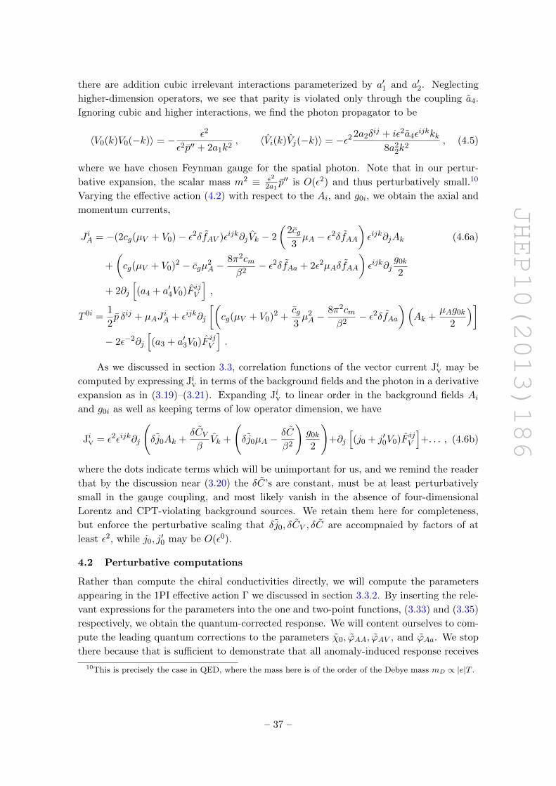
JHEP10(2013)186
there are addition cubic irrelevant interactions parameterized by a′1 and a′2. Neglecting
higher-dimension operators, we see that parity is violated only through the coupling a4.
Ignoring cubic and higher interactions, we find the photon propagator to be
〈V0(k)V0(−k)〉 = − ε2
ε2p′′ + 2a1k2, 〈Vi(k)Vj(−k)〉 = −ε2 2a2δ
ij + iε2a4εijkkk
8a22k
2, (4.5)
where we have chosen Feynman gauge for the spatial photon. Note that in our pertur-
bative expansion, the scalar mass m2 ≡ ε2
2a1p′′ is O(ε2) and thus perturbatively small.10
Varying the effective action (4.2) with respect to the Ai, and g0i, we obtain the axial and
momentum currents,
J iA = −(2cg(µV + V0)− ε2δfAV )εijk∂j Vk − 2
(2cg3µA − ε2δfAA
)εijk∂jAk (4.6a)
+
(cg(µV + V0)2 − cgµ2
A −8π2cmβ2
− ε2δfAa + 2ε2µAδfAA
)εijk∂j
g0k
2
+ 2∂j
[(a4 + a′4V0)F ijV
],
T 0i =1
2p δij + µAJ
iA + εijk∂j
[(cg(µV + V0)2 +
cg3µ2A −
8π2cmβ2
− ε2δfAa)(
Ak +µAg0k
2
)]− 2ε−2∂j
[(a3 + a′3V0)F ijV
].
As we discussed in section 3.3, correlation functions of the vector current JiV may be
computed by expressing JiV in terms of the background fields and the photon in a derivative
expansion as in (3.19)–(3.21). Expanding JiV to linear order in the background fields Aiand g0i as well as keeping terms of low operator dimension, we have
JiV = ε2εijk∂j
(δj0Ak +
δCVβ
Vk +
(δj0µA −
δC
β2
)g0k
2
)+∂j
[(j0 + j′0V0)F ijV
]+. . . , (4.6b)
where the dots indicate terms which will be unimportant for us, and we remind the reader
that by the discussion near (3.20) the δC’s are constant, must be at least perturbatively
small in the gauge coupling, and most likely vanish in the absence of four-dimensional
Lorentz and CPT-violating background sources. We retain them here for completeness,
but enforce the perturbative scaling that δj0, δCV , δC are accompnaied by factors of at
least ε2, while j0, j′0 may be O(ε0).
4.2 Perturbative computations
Rather than compute the chiral conductivities directly, we will compute the parameters
appearing in the 1PI effective action Γ we discussed in section 3.3.2. By inserting the rele-
vant expressions for the parameters into the one and two-point functions, (3.33) and (3.35)
respectively, we obtain the quantum-corrected response. We will content ourselves to com-
pute the leading quantum corrections to the parameters χ0, ϕAA, ϕAV , and ϕAa. We stop
there because that is sufficient to demonstrate that all anomaly-induced response receives
10This is precisely the case in QED, where the mass here is of the order of the Debye mass mD ∝ |e|T .
– 37 –
JHEP10(2013)186
ji1(k) jj2(−k)
V0
Vkg g ji1(k) jj2(−k)
V0
Figure 1. The basic one-loop diagrams correcting the various chiral conductivities. The cross
denotes the P-violating vertex g in (4.9), and the solid dot indicates the P-preserving vertex g as
discussed in the text.
quantum corrections when U(1)V is gauged. As a byproduct we obtain the leading correc-
tions to the chiral vortical conductivity; the leading order O(e2) term has recently been
computed in QED in [21, 22]. We discuss the matching between the two in section 4.3.
We work to low order in perturbation theory in the former expansion parameter ε.
By the power counting we imposed in the previous subsection, we see that intermediate
spatial photons introduce a factor of ε2, while intermediate V0’s introduce a factor of ε
that depends on whether V0 appears in a tree-level exchange or inside of a loop. When V0
appears in a tree-level exchange, its propagator is O(ε0) at low momentum. Inside a loop,
the V0 propagator introduces at least one additional factor of ε.
Let us now determine the ε-counting for diagrams which contribute to the two-point
functions of the axial, momentum, and vector currents (4.6). Since the interaction vertices
a′1, a′2, a4 are O(ε0), a diagram with nT tree-level V0’s, n0 intermediate V0’s inside a loop,
nV spatial photons, and O(ε0) operator insertions then scales at minimum with a factor
of εn0+2nV . Insertions with a δf , δj0 or δC introduce an extra factor of O(ε2), while
insertions with a factor of a3 or a′3 introduce a factor of O(ε−2).
4.2.1 Corrections to χ0
The parameters δj0 and χ0 appearing in (3.20), (3.33) control the response of the vector
current to the source for the axial current. As they explicitly violate U(1)A symmetry, they
are both at least O(ε2) in our formal power counting, which upon rescaling δj0 becomes
χ0 = ε2 δj0 +O(ε4) . (4.7)
The leading quantum corrections to χ0 then come from two one-loop diagrams. Since
we are computing O(k) terms in the effective action, we only consider the O(k) parts of
the relevant diagrams. The first loop has a V0 and Vi in the virtual intermediate state
connecting the vertices
JiV = . . .+ ∂j(j′0V0F
ijV ) + . . . , J iA = . . .− 2cgV0ε
ijk∂j Vk + . . . . (4.8)
The second diagram at this order is a V0V0 bubble arising from the vertex ε2δj′′0 appearing
in the vector current.
These are the essential one-loop diagrams that appear when computing χ0 as well
as the ϕ’s, albeit with different couplings in each case. Both diagrams are depicted in
– 38 –
JHEP10(2013)186
figure 1. As a result we evaluate the loops with arbitrary couplings and then insert the
relevant couplings when evaluating the parameters of Γ. Beginning with the V0Vi loop we
consider two currents j1 and j2 with
ji1 = ∂j(gV0FijV ) , ji2 = gV0ε
ijk∂j Vk . (4.9)
At low momentum we have
〈ji1(k)jj2(−k)〉V0V = iε4gg
8a1a2β
∫d3p
(2π)3
1
p2
1
p2 +m2
(piεjklpj − εijkpkpl
)kl +O(ε6, k2) ,
= −iε4 gg
12a1a2βεijkkk
(∫d3p
(2π)3
1
p2 +m2
)+O(ε6, k2) , (4.10)
wherem2 = ε2
2a1p′′ is the scalar mass. The terms ofO(ε6) and higher come from perturbative
corrections to the propagators involving a4 and higher derivative operators. The integral in
the second line is linearly divergent and so we regulate it with a hard UV cutoff Λ, giving11
〈ji1(k)jj2(−k)〉V0V = −iε4 ggT
24π2a1a2εijkkk
(Λ− π|m|
2+O
(m2
Λ
))+O(ε6, k2) , (4.11)
Note that since m ∼ O(ε) the subleading corrections in the Λ → ∞ limit are O(ε6), and
so may be consistently neglected to this order.
The V0V0 bubble arises from a vertex
ji1 = εijk∂j
(1
2g′′V 2
0 Ak
), (4.12)
where we treat Ak as a source for jk2 . The resulting bubble gives
〈ji1(k)jj2(−k)〉V0V0 = iε2g′′
4a1βεijkkk
∫d3p
(2π)3
1
p2 +m2+O(k2, ε4) ,
= iε2g′′T
8π2a1εijkkk
(Λ− π|m|
2
)+O(k2, ε4) ,
(4.13)
where we have again imposed a hard UV cutoff. For the case at hand we substitute
g = j′0, g = −2cg, and g′′ = ε2δj′′0 , and upon noting how χ0 appears in (3.35), we find
χ0 = ε2δj0 −ε4T
4π2a1
[j′0cg3a2
+δj′′02
](Λ− π|m|
2
)+O(ε6) . (4.14)
The two contributions in (4.11) can be interpreted as follows. The power-like UV
divergence is a consequence of the irrelevant interactions, and reflects the physics of the
nonzero Matsubara modes that are integrated out in obtaining the spatial effective theory.
This term needs to be matched to a specific UV completion. The second finite term,
proportional to |m| is non-analytic in the coupling and reflects the IR physics described
by the effective theory. It is independent of the precise UV completion, other than the
matching required to fix the infrared parameters.
11Although a fixed momentum cutoff is generally inconsistent with the U(1)V vector Ward identity, it is
acceptable here as we will not need to shift the loop momentum in the integral. We retain the power-like
divergences to highlight the appearance of terms which, after matching to the four-dimensional theory, are
associated with the nonzero Matsubara modes and can arise at leading order in perturbation theory.
– 39 –
JHEP10(2013)186
4.2.2 Corrections to ϕAA
The parameter ϕAA, which controls the response of the axial current to the source for the
axial current, is
ϕAA = −2cg3µA + ε2δfAA + (loops) . (4.15)
The leading loop corrections to it arise from a V0Vi loop of the form (4.11) as well as
a V0V0 bubble. Actually, the V0Vi loop is twice (4.11) (owing to the fact that that the
j1 = j2 = JA) with the identification g = 2a′4 and g = −2cg. There is also a V0V0 bubble
of the form (4.13) with g′′ = 2ε2δf ′′AA. Combining the loops and noting how ϕAA appears
in the axial-axial two-point function (3.35) we find
ϕAA = −2cg3µA + ε2δfAA −
ε4T
2π2a1
[a′4cg3a2
+δf ′′AA
4
](Λ− π|m|
2
)+O(ε6) . (4.16)
4.2.3 Corrections to ϕAV
The response of the axial current to a magnetic field is controlled by the parameter ϕAV ,
which is given by
ϕAV = −2cgµV + ε2δfAV + (loops) . (4.17)
Just as for χ0 and ϕAA, the leading corrections arise from a V0Vi loop of the form (4.11) as
well as the V0V0 bubble. In terms of the loops (4.11) and (4.13) we identify g = 4a′2, g =
−2cg and g′′ = ε2δfAV . Putting the loops together we find
ϕAV = −2cgµV + ε2δfAV −ε4T
π2a1
[a′2cg3a2
+δf ′′AV
8
](Λ− π|m|
2
)+O(ε6) . (4.18)
4.2.4 Corrections to ϕAa
At zero axial chemical potential, the parameter ϕAa governs the response of the axial
current to vorticity. It is
ϕAa = −cgµ2V −
cg3µ2A − 8π2cmT
2 + ε2δfAa + (loops) . (4.19)
Like the leading corrections to χ0 and the other ϕ’s, the lowest order quantum corrections
arise from a V0Vi loop of the form (4.11) as well as a V0V0 bubble. Unlike the corrections
above which were at least O(ε4), these are O(ε2). There are two V0Vi loops: in the first
we identify ji1 = J iA, jj2 = T 0j along with g = 2a′4 and g = −2cgµA, and in the second we
identify ji1 = T 0i, jj2 = J jA along with g = −2(ε−2a′3 − a′4µA) as well as g = −2cg. The
first loop is O(ε4) while the second is O(ε2). The V0V0 loop is of the form (4.13) with an
coupling g′′ = 2cg. The end result is
ϕAa = −cgµ2V −
cg3µ2A − 8π2cmT
2 + ε2(δfAa −
cgT
2π2a1
[a′33a2− 1
2
](Λ− π|m|
2
))+O(ε4) .
(4.20)
– 40 –
JHEP10(2013)186
4.2.5 Summary of the one-loop corrections
In section 3.3.2 we discussed the thermal effective action Γ and 1PI vector current. We
have calculated the leading quantum corrections to the one-derivative parts of Γ and the
vector current that involve the epsilon-tensor. From the previous subsection we find
χ0 = ε2δj0 −ε4T
4π2a1
[j′0cg3a2
+δj′′02
](Λ− π|m|
2
)+O(ε6) ,
ϕAA = −2cg3µA + ε2δfAA −
ε4T
2π2a1
[a′4cg3a2
+δf ′′AA
4
](Λ− π|m|
2
)+O(ε6) ,
ϕAV = −2cgµV + ε2δfAV −ε4T
π2a1
[a′2cg3a2
+δf ′′AV
8
](Λ− π|m|
2
)+O(ε6) , (4.21)
ϕAa = −cgµ2V −
cg3µ2A − 8π2cmT
2 + ε2(δfAa −
cgT
2π2a1
[a′33a2− 1
2
](Λ− π|m|
2
))+O(ε4) .
Since the effective theory has no fermionic matter and the theory is IR finite, the Chern-
Simons couplings are uncorrected to all orders in perturbation theory,
cAA = cAV = cV V = cV = c = CV = C = 0 . (4.22)
We observe that the structure of (4.21) indicates that the leading corrections to χ0, ϕAA,
and ϕAV are in fact O(ε4) rather than O(ε2). Upon inserting the 1PI parameters (4.21)
back into (3.35), we obtain the leading corrections to the two-point functions of the vector,
axial, and momentum currents.
4.3 Matching to the four-dimensional theory
The loop corrections to the chiral vortical conductivity contain power-like UV divergences
at O(ε2), which need to be matched at the cutoff scale (Λ . T ) with the full four-
dimensional theory. The spatial EFT can only be used to reliably compute the non-analytic
subleading corrections of O(ε2|ε|). In this subsection, we relate our perturbative calcula-
tions of the CVE in the EFT to four-dimensional calculations in QED with Nf Dirac
fermions. The leading quantum corrections to the CVE in QED to O(e2) at µV = µA = 0
have been discussed in [21, 22]. In this case the anomaly coefficients are
cg = −Nf
4π2, cg = −Nf
4π2, cm = − Nf
96π2. (4.23)
We will now compute the chiral vortical conductivity σCV E in QED, defined through
i
2limk→0
εijlkl
k2〈J iA(k)T 0j(−k)〉 = σCV E . (4.24)
For simplicity we will also work at zero chemical potentials, µV = µA = 0. In (3.35) we
showed how σCV E is related to the parameters appearing in the thermal effective action
Γ and the 1PI vector current. To proceed we require knowledge of the ϕ’s, α2, α3, α4, and
α4. For QED we have
α2 = − 1
4e2+O(e0) , (4.25)
– 41 –
JHEP10(2013)186
and the combination of charge conjugation and parity symmetry sets
α3 = α4 = α4 = 0 , (4.26)
which by (3.35) gives
σCV E = −ϕAa . (4.27)
In (4.21) we expressed ϕAa in terms of the parameters of the Wilsonian effective action
Seff , which upon using
a1 =1
2e2+O(e0) , a2 = − 1
4e2+O(e0) , a′3 = − 1
2e2+O(e0) , (4.28)
gives
σCV E = −ϕAa = −NfT2
24− e2δfAa −
e2NfT
24π4
(Λ− π|m|
2
)+O(e4) . (4.29)
The O(e2) part of the CVE depends on the UV cutoff and the parameter δfAa, and so
is determined by matching to the UV theory in question, in this case QED. The term
proportional to |m| is an IR-sensitive O(e2|e|) term which is independent of the details of
the UV completion.
It is interesting to explore the origin of this correction directly in four dimensions.
Indeed, the corresponding O(e2) contributions to δfAa were recently studied in [21, 22],
and arise via two-loop contributions to 〈J iAT 0j〉. In the Matsubara formalism, to compare
with the effective theory calculation we can isolate the zero-modes n = 0,
δσCV E = δσn=0CV E + δσn 6=0
CV E . (4.30)
In the analysis of [21, 22], the relevant diagram factorizes into a triangle anomaly
(AV V ) sub-diagram, and the use of an effective anomaly-induced axial vertex reduces the
computation to two one-loop photon bubble diagrams. However, only one of these has
a nonzero contribution from the zero modes, involving a V0Vj loop. The effective axial
current vertex for the zero modes used in [21, 22] takes the form Γ0ji = −Γj0i = cgεijkpk,
where ~p is the spatial loop momentum. At leading order the zero mode contribution
is T -independent, and the O(e2) contribution to δfAa arises as expected only from the
nonzero modes δσn6=0CV E . However, the IR contribution of the zero mode becomes nontrivial
on resumming the 〈V0V0〉 propagator to incorporate the effect of Debye screening. In
particular, if we resum the photon self-energy, the propagator for the zero mode of
V0 is modified as 1/p2 → 1/(p2 + m2), and incorporates the Debye mass m2. Since
m2 = O(e2T 2) T 2 it is consistent to resum the zero mode propagator, and neglect the
corresponding corrections to the nonzero modes. With this resummation, we find
δσn=0CV E = −e
2NfT
12π2
∫d3~p
(2π)3
1
~p2 +m2= −e
2NfT
24π4[Λ−m arctan(Λ/m)]Λ→∞
= O(Λ) +e2NfT
48π3|m|. (4.31)
– 42 –
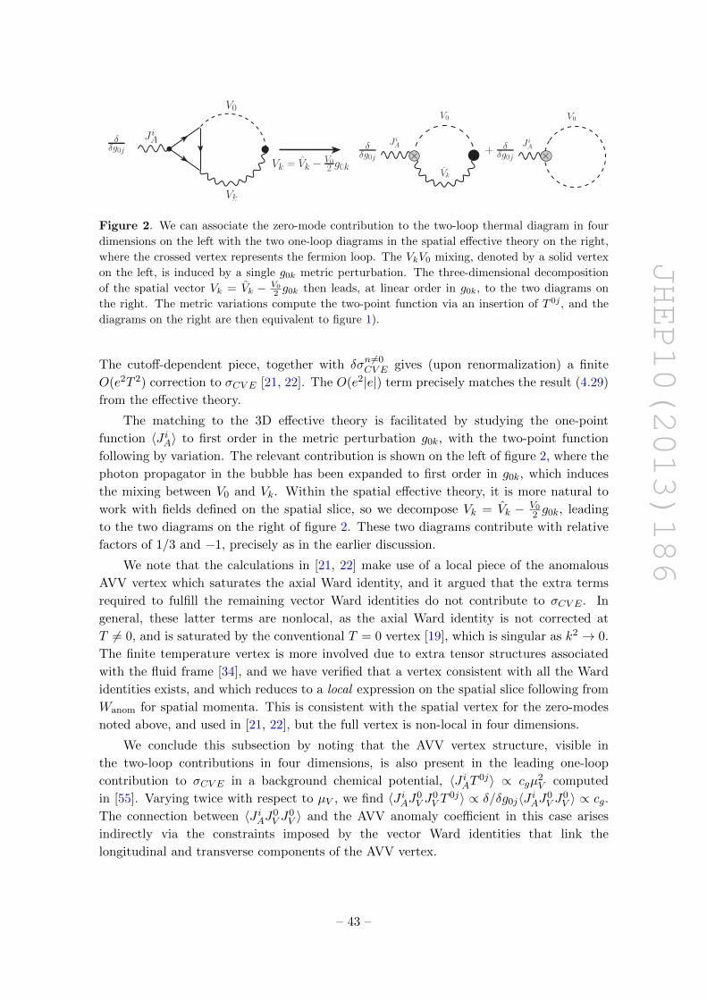
JHEP10(2013)186
J iAδδg0j
V0
Vk = Vk − V02 g0k
Vk
+ δδg0j
δδg0j
J iA
V0
J iA
V0
Vk
Figure 2. We can associate the zero-mode contribution to the two-loop thermal diagram in four
dimensions on the left with the two one-loop diagrams in the spatial effective theory on the right,
where the crossed vertex represents the fermion loop. The VkV0 mixing, denoted by a solid vertex
on the left, is induced by a single g0k metric perturbation. The three-dimensional decomposition
of the spatial vector Vk = Vk − V0
2 g0k then leads, at linear order in g0k, to the two diagrams on
the right. The metric variations compute the two-point function via an insertion of T 0j , and the
diagrams on the right are then equivalent to figure 1).
The cutoff-dependent piece, together with δσn6=0CV E gives (upon renormalization) a finite
O(e2T 2) correction to σCV E [21, 22]. The O(e2|e|) term precisely matches the result (4.29)
from the effective theory.
The matching to the 3D effective theory is facilitated by studying the one-point
function 〈J iA〉 to first order in the metric perturbation g0k, with the two-point function
following by variation. The relevant contribution is shown on the left of figure 2, where the
photon propagator in the bubble has been expanded to first order in g0k, which induces
the mixing between V0 and Vk. Within the spatial effective theory, it is more natural to
work with fields defined on the spatial slice, so we decompose Vk = Vk − V02 g0k, leading
to the two diagrams on the right of figure 2. These two diagrams contribute with relative
factors of 1/3 and −1, precisely as in the earlier discussion.
We note that the calculations in [21, 22] make use of a local piece of the anomalous
AVV vertex which saturates the axial Ward identity, and it argued that the extra terms
required to fulfill the remaining vector Ward identities do not contribute to σCV E . In
general, these latter terms are nonlocal, as the axial Ward identity is not corrected at
T 6= 0, and is saturated by the conventional T = 0 vertex [19], which is singular as k2 → 0.
The finite temperature vertex is more involved due to extra tensor structures associated
with the fluid frame [34], and we have verified that a vertex consistent with all the Ward
identities exists, and which reduces to a local expression on the spatial slice following from
Wanom for spatial momenta. This is consistent with the spatial vertex for the zero-modes
noted above, and used in [21, 22], but the full vertex is non-local in four dimensions.
We conclude this subsection by noting that the AVV vertex structure, visible in
the two-loop contributions in four dimensions, is also present in the leading one-loop
contribution to σCV E in a background chemical potential, 〈J iAT 0j〉 ∝ cgµ2V computed
in [55]. Varying twice with respect to µV , we find 〈J iAJ0V J
0V T
0j〉 ∝ δ/δg0j〈J iAJ0V J
0V 〉 ∝ cg.
The connection between 〈J iAJ0V J
0V 〉 and the AVV anomaly coefficient in this case arises
indirectly via the constraints imposed by the vector Ward identities that link the
longitudinal and transverse components of the AVV vertex.
– 43 –
JHEP10(2013)186
5 Discussion
In this work we sought to understand the fate of anomaly-induced transport with dy-
namical gauge fields. Our results are summarized in section 1, and are captured in the
derivative expansion for the effective action (3.11)–(3.16), and the two-point functions of
currents (3.35), (3.37) that determine the appearance of the anomaly coefficients in hy-
drostatic response. We find that anomaly-induced transport is subject to perturbative
corrections. We explicitly studied one-loop contributions to the spatial effective action,
reproducing for example IR-sensitive corrections to the chiral vortical conductivity.
In the remainder of this section, we comment on the chiral magnetic effect, magnetohy-
drodynamics, and the application of these results to the Standard Model, necessarily focus-
ing on perturbative regimes in which the corrections to anomalous transport remain small.
• Axial chemical potential : discussions of anomalous transport often involve the axial
chemical potential. However, in the presence of dynamical U(1)V fields, this is a
subtle quantity to define in equilibrium. We have made use of the source µA for the
axial charge QA =∫d3xJ0
A, but this is not a true chemical potential, since QA is not
conserved. However, in the presence of the AV V anomaly, one can define a conserved
axial charge Q5 =∫d3x(J0
A − cgε0ijkVi∂jVk) [32] (at least when the field strength
of the axial source, (FA)µν vanishes). The corresponding current is not U(1)V gauge
invariant, but the charge Q5 is invariant, and one can consider a time-independent
thermal ensemble defined by H − µ5Q5, with µ5 now interpreted as a genuine axial
chemical potential. We now consider the implications of this source when U(1)V is
dynamical. Indeed, within the spatial effective theory, the presence of this source
leads to cV V = −2cgµ5. This has the effect of shifting the static pole of the spatial
photon away from zero, leading to anti-screening [64, 65] (see also the recent discus-
sion in [66, 68]). If this constant value of µ5 is realized in terms of a dynamical field,
this anti-screening observed on the spatial slice likely implies a dynamical instability.
One method to obtain an axial chemical potential µ5 is to turn on a four-dimensional
axion coupling aFµνFµν with an axion profile linear in time a ∝ t, so that µ5 ∝ ∂ta.
In this case, there is indeed an unstable growing mode for the magnetic field, and
thus a consistent treatment would involve the full non-equilibrium dynamics.
• Chiral magnetic effect : the chiral magnetic effect [9–12] can be understood quali-
tatively as a contribution to the electromagnetic current aligned along an external
magnetic field. However, the precise realization depends on the definition of the
current and whether the U(1)V field is dynamical. We consider first the case of a
global (i.e. external) U(1)V magnetic field. In the presence of the AV V anomaly
and the source µA, the consistent and covariant currents differ by a Bardeen-Zumino
polynomial which is precisely of the form required to shift the coefficient of the
‘CME-like’ relation J iV,cov ∝ µABi. However, this coefficient depends on whether
one considers the covariant or consistent current, and indeed it vanishes for the
U(1)V -invariant consistent current. The recent literature [11, 12, 32] has discussed
a more precise relation to the AV V anomaly, which emerges when working with
– 44 –
JHEP10(2013)186
the true axial chemical potential µ5 discussed above. The additional Chern-Simons
term in Q5 then ensures that the consistent current takes the chiral magnetic form,
J iV = −2cgµ5Bi, with the relation to the anomaly fixed by the unique definition of
µ5 as conjugate to the conserved axial charge.
When the U(1)V field is dynamical, we are forced to work with the U(1)V -invariant
consistent currents and thus the source µA does not lead to the CME [32]. If
one allows for additional constant CPT-odd sources, then a CME-like relation
for the current can arise. For example, in (3.30) we have 〈JiV〉 = CV TBi, where
Bi = εijk〈FV,jk〉/2 is the magnetic field, determined by Jext and other external
sources. The coefficient CV is a CPT-odd constant, which needs to be fixed by
matching to the UV theory, and is not a priori dictated by anomalies. A more precise
relation between CV and the AVV anomaly may emerge (although the anomalous
symmetry does not relate the two) when we study a particular theory where we can
keep track of the CPT-violating sources, like µ5 [32, 69]. However, when U(1)V is
dynamical, as discussed above we find cV V = −2cgµ5 which results in anti-screening
of the magnetic field, and likely a dynamical instability. This suggests that any
consistent treatment of the CME in the presence of dynamical gauge fields must go
beyond an equilibrium framework (see e.g. [70]).
• Magnetohydrodynamics: in this paper our primary focus was the impact of anomalies
on hydrostatic response. However, our analysis was motivated by an attempt to
understand the constraints that equilibrium matching imposes on hydrodynamics.
Thus in section 3.2, we briefly discussed the structure of hydrodynamics with
dynamical (but classical) U(1)V gauge fields, i.e. magnetohydrodynamics. Note that
this is not quite textbook MHD, in that we treated the magnetic field as a first-order
quantity in the derivative expansion. It would clearly be of interest to develop this
framework further, to take anomalies into account at the level of effective field theory,
and make contact with existing approaches [71]. It may also prove worthwhile to
study the form of constitutive relations using the fluid-gravity framework within
AdS/CFT. The framework of section 3 should also describe holographic examples
with dynamical U(1)V gauge fields, including the alternate quantization of a bulk
gauge field in asymptotically AdS4 spacetimes [72] and the standard quantization in
AdS3 backgrounds [72, 73].
• Quark-gluon plasma: the U(Nf )L × U(Nf )R chiral currents in QCD decompose
into non-singlet SU(Nf )A and singlet U(1)A axial currents. The latter U(1) current
receives a large gluonic contribution to the anomaly (associated with mass of the η′
meson), implying that the degrees of freedom associated with this current are not ex-
pected to contribute in the hydrodynamic regime. However, the non-singlet currents
have purely electromagnetic anomalies, allowing for a quantitative identification of
anomaly-induced physics, e.g. the rate for π0 → γγ decays. In this case, the presence
of small perturbative corrections that we have discussed here should not significantly
modify the notion of anomalous transport. The extension of the present work to
– 45 –
JHEP10(2013)186
Cartan components of the non-abelian axial global currents is straightforward, and
may be of interest for the study of anomalous transport in the quark-gluon plasma.
• Mixed anomalies: when the mixed gauge-gravitational anomaly (2.43) is nonzero,
it will provide the primary contribution to the chiral vortical response at sufficiently
high temperatures via the T 2 term in (2.27). Currents with non-vanishing mixed
anomalies are therefore particular interest as they may exhibit an enhanced chiral
vortical conductivity as a macroscopic manifestation of this anomaly. The chiral
lepton number current is an example, and early cosmology may provide a high
temperature regime in which the mixed gauge-gravitational anomaly could play
a role. We recall that the conventional electroweak VB+LAV anomaly of the
vectorial U(1)B+L baryon plus lepton number current in the Standard Model is the
only source of baryon and lepton number violation in the Standard Model. The
associated sphaleron transitions above the electroweak scale have been utilized in
various models of baryogenesis. It would be interesting if the mixed anomaly for the
chiral lepton current were also to play a cosmological role.
• Additional gapless modes: we have discussed the corrections to anomaly-induced
transport that arise when the vector symmetry is gauged. Another way that
anomaly-induced response may differ from section 2.2 is through the presence
of additional gapless modes which contribute to hydrostatic response. Examples
discussed in the literature include a U(1) superfluid, and QED at zero temper-
ature and nonzero chemical potential. In a U(1) superfluid there is an extra
massless Goldstone mode φ, and additional gauge-invariant scalars εijkDiφ∂jAkand εijkDiφ∂jak, where Diφ = ∂iφ − Ai, which give rise to magnetic and vortical
response beyond the anomalies [67]. In zero temperature QED there is a sharp
Fermi surface, and a recent two-loop calculation [74] has shown that the Fermi
surface leads to a correction to the Chiral Separation Effect, (i.e. the O(k) part of
the two-point function 〈J iV (k)J jA(−k)〉), which in the presence of screening is fixed
by anomalies [8]. In summary, we can categorize the corrections to anomaly-induced
response as due to the dynamics of (e.g. gauge) fields entering the anomaly vertex,
and/or the breakdown of screening and the presence of additional gapless modes.
Acknowledgments
We would like to thank S. Golkar, C. Hoyos, M. Kaminski, D. Kharzeev, R. Loganayagam,
M. Pospelov, I. Shovkovy, D. Son, L. Yaffe, and A. Yarom for useful discussions and/or
comments on the manuscript. This work was supported in part by NSERC, Canada.
References
[1] S. Weinberg, The quantum theory of fields. Volume 2: modern applications, Cambridge
University Press, Cambridge U.K. (1996) [INSPIRE].
– 46 –
JHEP10(2013)186
[2] D.T. Son and P. Surowka, Hydrodynamics with triangle anomalies, Phys. Rev. Lett. 103
(2009) 191601 [arXiv:0906.5044] [INSPIRE].
[3] Y. Neiman and Y. Oz, Relativistic hydrodynamics with general anomalous charges, JHEP 03
(2011) 023 [arXiv:1011.5107] [INSPIRE].
[4] K. Jensen, R. Loganayagam and A. Yarom, Thermodynamics, gravitational anomalies and
cones, JHEP 02 (2013) 088 [arXiv:1207.5824] [INSPIRE].
[5] D. Son and A.R. Zhitnitsky, Quantum anomalies in dense matter, Phys. Rev. D 70 (2004)
074018 [hep-ph/0405216] [INSPIRE].
[6] I. Amado, K. Landsteiner and F. Pena-Benitez, Anomalous transport coefficients from Kubo
formulas in holography, JHEP 05 (2011) 081 [arXiv:1102.4577] [INSPIRE].
[7] N. Banerjee et al., Constraints on fluid dynamics from equilibrium partition functions, JHEP
09 (2012) 046 [arXiv:1203.3544] [INSPIRE].
[8] K. Jensen, Triangle anomalies, thermodynamics and hydrodynamics, Phys. Rev. D 85 (2012)
125017 [arXiv:1203.3599] [INSPIRE].
[9] A. Vilenkin, Equilibrium parity violating current in a magnetic field, Phys. Rev. D 22 (1980)
3080 [INSPIRE].
[10] A.Y. Alekseev, V.V. Cheianov and J. Frohlich, Universality of transport properties in
equilibrium, Goldstone theorem and chiral anomaly, Phys. Rev. Lett. 81 (1998) 3503
[cond-mat/9803346] [INSPIRE].
[11] K. Fukushima, D.E. Kharzeev and H.J. Warringa, The chiral magnetic effect, Phys. Rev. D
78 (2008) 074033 [arXiv:0808.3382] [INSPIRE].
[12] D.E. Kharzeev and H.J. Warringa, Chiral magnetic conductivity, Phys. Rev. D 80 (2009)
034028 [arXiv:0907.5007] [INSPIRE].
[13] A. Vilenkin, Cancellation of equilibrium parity violating currents, Phys. Rev. D 22 (1980)
3067 [INSPIRE].
[14] M.A. Metlitski and A.R. Zhitnitsky, Anomalous axion interactions and topological currents
in dense matter, Phys. Rev. D 72 (2005) 045011 [hep-ph/0505072] [INSPIRE].
[15] G. Newman and D. Son, Response of strongly-interacting matter to magnetic field: some
exact results, Phys. Rev. D 73 (2006) 045006 [hep-ph/0510049] [INSPIRE].
[16] A. Vilenkin, Macroscopic parity violating effects: neutrino fluxes from rotating black holes
and in rotating thermal radiation, Phys. Rev. D 20 (1979) 1807 [INSPIRE].
[17] V.I. Zakharov, Chiral magnetic effect in hydrodynamic approximation, Lect. Notes Phys. 871
(2013) 295 [arXiv:1210.2186] [INSPIRE].
[18] S.L. Adler and W.A. Bardeen, Absence of higher order corrections in the anomalous axial
vector divergence equation, Phys. Rev. 182 (1969) 1517 [INSPIRE].
[19] S.L. Adler, Axial vector vertex in spinor electrodynamics, Phys. Rev. 177 (1969) 2426
[INSPIRE].
[20] S.L. Adler, Anomalies to all orders, hep-th/0405040 [INSPIRE].
[21] S. Golkar and D.T. Son, Non-renormalization of the chiral vortical effect coefficient,
arXiv:1207.5806 [INSPIRE].
– 47 –
JHEP10(2013)186
[22] D.-F. Hou, H. Liu and H.-C. Ren, A possible higher order correction to the vortical
conductivity in a gauge field plasma, Phys. Rev. D 86 (2012) 121703 [arXiv:1210.0969]
[INSPIRE].
[23] P. Kovtun, G.D. Moore and P. Romatschke, The stickiness of sound: an absolute lower limit
on viscosity and the breakdown of second order relativistic hydrodynamics, Phys. Rev. D 84
(2011) 025006 [arXiv:1104.1586] [INSPIRE].
[24] E. Braaten and A. Nieto, Effective field theory approach to high temperature
thermodynamics, Phys. Rev. D 51 (1995) 6990 [hep-ph/9501375] [INSPIRE].
[25] E. Braaten and A. Nieto, Free energy of QCD at high temperature, Phys. Rev. D 53 (1996)
3421 [hep-ph/9510408] [INSPIRE].
[26] J.O. Andersen, The free energy of high temperature QED to order e5 from effective field
theory, Phys. Rev. D 53 (1996) 7286 [hep-ph/9509409] [INSPIRE].
[27] K. Jensen et al., Towards hydrodynamics without an entropy current, Phys. Rev. Lett. 109
(2012) 101601 [arXiv:1203.3556] [INSPIRE].
[28] A. Niemi and G. Semenoff, Axial anomaly induced Fermion fractionization and effective
gauge theory actions in odd dimensional space-times, Phys. Rev. Lett. 51 (1983) 2077
[INSPIRE].
[29] A. Redlich, Parity violation and gauge noninvariance of the effective gauge field action in
three-dimensions, Phys. Rev. D 29 (1984) 2366 [INSPIRE].
[30] S.R. Coleman and B.R. Hill, No more corrections to the topological mass term in QED in
three-dimensions, Phys. Lett. B 159 (1985) 184 [INSPIRE].
[31] J.C. Collins, A.V. Manohar and M.B. Wise, Renormalization of the vector current in QED,
Phys. Rev. D 73 (2006) 105019 [hep-th/0512187] [INSPIRE].
[32] V. Rubakov, On chiral magnetic effect and holography, arXiv:1005.1888 [INSPIRE].
[33] V. Braguta, M. Chernodub, K. Landsteiner, M. Polikarpov and M. Ulybyshev, Numerical
evidence of the axial magnetic effect, arXiv:1303.6266 [INSPIRE].
[34] H. Itoyama and A.H. Mueller, The axial anomaly at finite temperature, Nucl. Phys. B 218
(1983) 349 [INSPIRE].
[35] R.A. Bertlmann, Anomalies in quantum field theory, Clarendon Press, Oxford U.K. (1996)
[INSPIRE].
[36] J.A. Harvey, TASI 2003 lectures on anomalies, hep-th/0509097 [INSPIRE].
[37] A. Bilal, Lectures on anomalies, arXiv:0802.0634 [INSPIRE].
[38] J. Wess and B. Zumino, Consequences of anomalous Ward identities, Phys. Lett. B 37
(1971) 95 [INSPIRE].
[39] W.A. Bardeen and B. Zumino, Consistent and covariant anomalies in gauge and
gravitational theories, Nucl. Phys. B 244 (1984) 421 [INSPIRE].
[40] L.D. Landau and E.M. Lifshitz, Fluid mechanics, Pergamon Press, Oxford U.K. (1987).
[41] S. Bhattacharyya, V.E. Hubeny, S. Minwalla and M. Rangamani, Nonlinear fluid dynamics
from gravity, JHEP 02 (2008) 045 [arXiv:0712.2456] [INSPIRE].
– 48 –
JHEP10(2013)186
[42] R. Baier, P. Romatschke, D.T. Son, A.O. Starinets and M.A. Stephanov, Relativistic viscous
hydrodynamics, conformal invariance and holography, JHEP 04 (2008) 100
[arXiv:0712.2451] [INSPIRE].
[43] E. Wang and U.W. Heinz, A generalized fluctuation dissipation theorem for nonlinear
response functions, Phys. Rev. D 66 (2002) 025008 [hep-th/9809016] [INSPIRE].
[44] G.D. Moore and K.A. Sohrabi, Kubo formulae for second-order hydrodynamic coefficients,
Phys. Rev. Lett. 106 (2011) 122302 [arXiv:1007.5333] [INSPIRE].
[45] J. Erdmenger, M. Haack, M. Kaminski and A. Yarom, Fluid dynamics of R-charged black
holes, JHEP 01 (2009) 055 [arXiv:0809.2488] [INSPIRE].
[46] N. Banerjee et al., Hydrodynamics from charged black branes, JHEP 01 (2011) 094
[arXiv:0809.2596] [INSPIRE].
[47] K. Jensen et al., Parity-violating hydrodynamics in 2 + 1 dimensions, JHEP 05 (2012) 102
[arXiv:1112.4498] [INSPIRE].
[48] S. Dubovsky, L. Hui and A. Nicolis, Effective field theory for hydrodynamics: Wess-Zumino
term and anomalies in two spacetime dimensions, arXiv:1107.0732 [INSPIRE].
[49] V. Nair, R. Ray and S. Roy, Fluids, anomalies and the chiral magnetic effect: a
group-theoretic formulation, Phys. Rev. D 86 (2012) 025012 [arXiv:1112.4022] [INSPIRE].
[50] T. Evans, N point finite temperature expectation values at real times, Nucl. Phys. B 374
(1992) 340 [INSPIRE].
[51] J. Bhattacharya, S. Bhattacharyya, S. Minwalla and A. Yarom, A theory of first order
dissipative superfluid dynamics, arXiv:1105.3733 [INSPIRE].
[52] R. Loganayagam, Anomaly induced transport in arbitrary dimensions, arXiv:1106.0277
[INSPIRE].
[53] D.E. Kharzeev and H.-U. Yee, Anomalies and time reversal invariance in relativistic
hydrodynamics: the second order and higher dimensional formulations, Phys. Rev. D 84
(2011) 045025 [arXiv:1105.6360] [INSPIRE].
[54] S. Bhattacharyya, J.R. David and S. Thakur, Second order transport from anomalies,
arXiv:1305.0340 [INSPIRE].
[55] K. Landsteiner, E. Megias and F. Pena-Benitez, Gravitational anomaly and transport, Phys.
Rev. Lett. 107 (2011) 021601 [arXiv:1103.5006] [INSPIRE].
[56] K. Landsteiner, E. Megias, L. Melgar and F. Pena-Benitez, Holographic gravitational
anomaly and chiral vortical effect, JHEP 09 (2011) 121 [arXiv:1107.0368] [INSPIRE].
[57] H. Bloete, J.L. Cardy and M. Nightingale, Conformal invariance, the central charge and
universal finite size amplitudes at criticality, Phys. Rev. Lett. 56 (1986) 742 [INSPIRE].
[58] I. Affleck, Universal term in the free energy at a critical point and the conformal anomaly,
Phys. Rev. Lett. 56 (1986) 746 [INSPIRE].
[59] S.N. Solodukhin, Entanglement entropy of black holes, Living Rev. Rel. 14 (2011) 8
[arXiv:1104.3712] [INSPIRE].
[60] R. Loganayagam, Anomalies and the helicity of the thermal state, arXiv:1211.3850
[INSPIRE].
– 49 –
JHEP10(2013)186
[61] J.I. Kapusta, Bose-Einstein condensation, spontaneous symmetry breaking and gauge
theories, Phys. Rev. D 24 (1981) 426 [INSPIRE].
[62] P.A. Davidson, An introduction to magnetohydrodynamics, Cambridge University Press,
Cambridge U.K. (2001).
[63] C. Closset, T.T. Dumitrescu, G. Festuccia, Z. Komargodski and N. Seiberg, Comments on
Chern-Simons contact terms in three dimensions, JHEP 09 (2012) 091 [arXiv:1206.5218]
[INSPIRE].
[64] A. Redlich and L. Wijewardhana, Induced Chern-Simons terms at high temperatures and
finite densities, Phys. Rev. Lett. 54 (1985) 970 [INSPIRE].
[65] A. Niemi and G. Semenoff, A comment on ‘induced Chern-Simons terms at high
temperatures and finite densities’, Phys. Rev. Lett. 54 (1985) 2166 [INSPIRE].
[66] Z. Khaidukov, V. Kirilin, A. Sadofyev and V. Zakharov, On magnetostatics of chiral media,
arXiv:1307.0138 [INSPIRE].
[67] S. Bhattacharyya, S. Jain, S. Minwalla and T. Sharma, Constraints on superfluid
hydrodynamics from equilibrium partition functions, JHEP 01 (2013) 040 [arXiv:1206.6106]
[INSPIRE].
[68] Y. Akamatsu and N. Yamamoto, Chiral plasma instabilities, Phys. Rev. Lett. 111 (2013)
052002 [arXiv:1302.2125] [INSPIRE].
[69] D. Hou, H. Liu and H.-C. Ren, Some field theoretic issues regarding the chiral magnetic
effect, JHEP 05 (2011) 046 [arXiv:1103.2035] [INSPIRE].
[70] H.J. Warringa, Dynamics of the chiral magnetic effect in a weak magnetic field, Phys. Rev.
D 86 (2012) 085029 [arXiv:1205.5679] [INSPIRE].
[71] X.-G. Huang, A. Sedrakian and D.H. Rischke, Kubo formulae for relativistic fluids in strong
magnetic fields, Annals Phys. 326 (2011) 3075 [arXiv:1108.0602] [INSPIRE].
[72] D. Marolf and S.F. Ross, Boundary conditions and new dualities: vector fields in AdS/CFT,
JHEP 11 (2006) 085 [hep-th/0606113] [INSPIRE].
[73] K. Jensen, Chiral anomalies and AdS/CMT in two dimensions, JHEP 01 (2011) 109
[arXiv:1012.4831] [INSPIRE].
[74] E. Gorbar, V. Miransky, I. Shovkovy and X. Wang, Radiative corrections to chiral separation
effect in QED, Phys. Rev. D 88 (2013) 025025 [arXiv:1304.4606] [INSPIRE].
– 50 –