Embed Size (px)
Citation preview
ChIP-seq
Peter N.Robinson
eigenstuff
SymmetricMatrices
Gene Reg.
PCA
Gene Reg.
ChIP-seqExpression Networks
Peter N. Robinson
Institut fur Medizinische Genetik und HumangenetikCharite Universitatsmedizin Berlin
Genomics: Lecture #14
ChIP-seq
Peter N.Robinson
eigenstuff
SymmetricMatrices
Gene Reg.
PCA
Gene Reg.
Gene Expression Networks
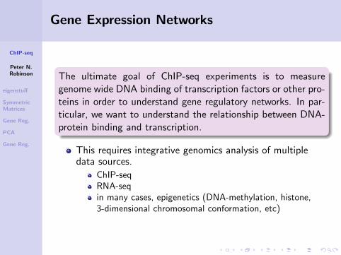
The ultimate goal of ChIP-seq experiments is to measuregenome wide DNA binding of transcription factors or other pro-teins in order to understand gene regulatory networks. In par-ticular, we want to understand the relationship between DNA-protein binding and transcription.
This requires integrative genomics analysis of multipledata sources.
ChIP-seqRNA-seqin many cases, epigenetics (DNA-methylation, histone,3-dimensional chromosomal conformation, etc)

ChIP-seq
Peter N.Robinson
eigenstuff
SymmetricMatrices
Gene Reg.
PCA
Gene Reg.
Sit back and enjoy
Today, we will talk about an integrated analysis of genomicsdata on many levels. Sit back and enjoy!
How to Do Good Bioinformatics for Genomics
1 Read mapping
2 Make calls about basic data (variants,isoforms, differential expression,structural variants, ChIP-seq peaks)
3 Integrative bioinformatics (and wetlabexperiments) to answer importantquestions about biology or medicine!
We have not yet covered (3) in this course, but it will be your challenge for the next decade!
ChIP-seq
Peter N.Robinson
eigenstuff
SymmetricMatrices
Gene Reg.
PCA
Gene Reg.
Gene Expression Networks
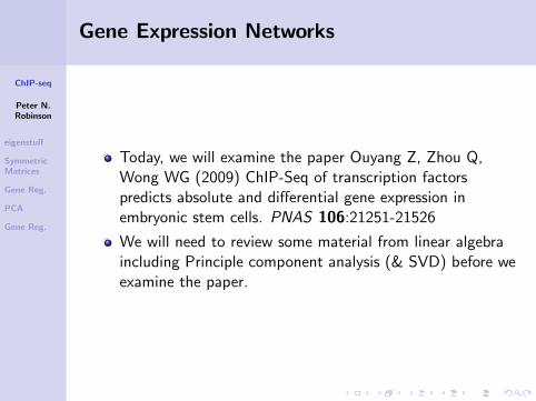
Today, we will examine the paper Ouyang Z, Zhou Q,Wong WG (2009) ChIP-Seq of transcription factorspredicts absolute and differential gene expression inembryonic stem cells. PNAS 106:21251-21526
We will need to review some material from linear algebraincluding Principle component analysis (& SVD) before weexamine the paper.

ChIP-seq
Peter N.Robinson
eigenstuff
SymmetricMatrices
Gene Reg.
PCA
Gene Reg.
Outline
1 Eigenvalues and Eigenvectors
2 Symmetric Matrices
3 Back to Gene Regulation
4 Principle Component Analysis (PCA)
5 Getting back again to gene regulation
ChIP-seq
Peter N.Robinson
eigenstuff
SymmetricMatrices
Gene Reg.
PCA
Gene Reg.
Linear algebra: quick review
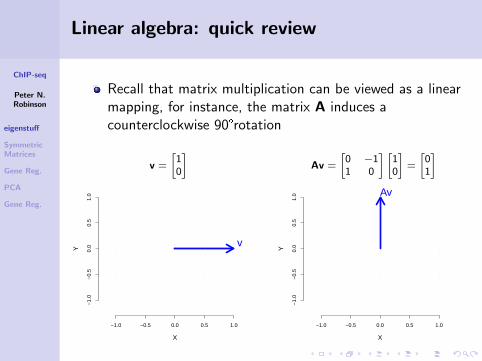
Recall that matrix multiplication can be viewed as a linearmapping, for instance, the matrix A induces acounterclockwise 90°rotation
v =
[10
]Av =
[0 −11 0
] [10
]=
[01
]
−1.0 −0.5 0.0 0.5 1.0
−1.
0−
0.5
0.0
0.5
1.0
X
Y
v
−1.0 −0.5 0.0 0.5 1.0
−1.
0−
0.5
0.0
0.5
1.0
X
Y
Av
ChIP-seq
Peter N.Robinson
eigenstuff
SymmetricMatrices
Gene Reg.
PCA
Gene Reg.
Linear algebra: quick review
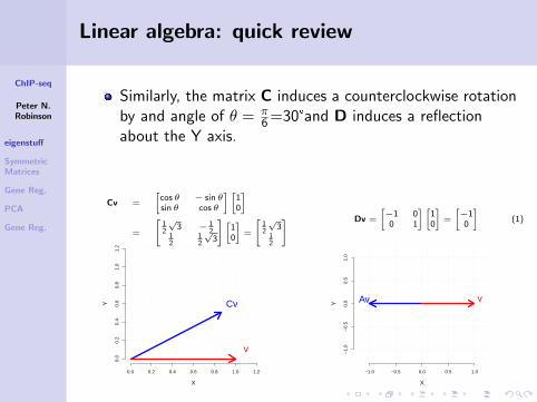
Similarly, the matrix C induces a counterclockwise rotationby and angle of θ = π
6 =30°and D induces a reflectionabout the Y axis.
Cv =
[cos θ − sin θsin θ cos θ
] [10
]
=
[12
√3 − 1
212
12
√3
] [10
]=
[12
√3
12
] Dv =
[−1 00 1
] [10
]=
[−10
](1)
0.0 0.2 0.4 0.6 0.8 1.0 1.2
0.0
0.2
0.4
0.6
0.8
1.0
1.2
X
Y Cv
v
−1.0 −0.5 0.0 0.5 1.0
−1.
0−
0.5
0.0
0.5
1.0
X
Y Av v
ChIP-seq
Peter N.Robinson
eigenstuff
SymmetricMatrices
Gene Reg.
PCA
Gene Reg.
Eigenvalues and eigenvectors
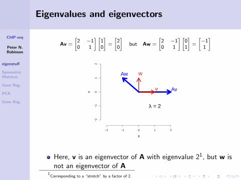
Av =
[2 −10 1
] [10
]=
[20
]but Aw =
[2 −10 1
] [01
]=
[−11
]
−2 −1 0 1 2
−2
−1
01
2
X
YAvv
wAw
λ = 2
Here, v is an eigenvector of A with eigenvalue 21, but w isnot an eigenvector of A
1Corresponding to a “stretch” by a factor of 2.
ChIP-seq
Peter N.Robinson
eigenstuff
SymmetricMatrices
Gene Reg.
PCA
Gene Reg.
Eigenvalues and eigenvectors
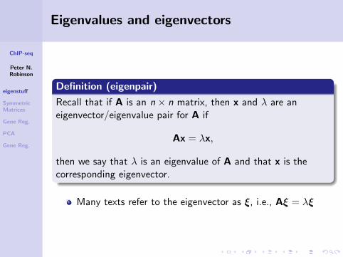
Definition (eigenpair)
Recall that if A is an n × n matrix, then x and λ are aneigenvector/eigenvalue pair for A if
Ax = λx,
then we say that λ is an eigenvalue of A and that x is thecorresponding eigenvector.
Many texts refer to the eigenvector as ξ, i.e., Aξ = λξ
ChIP-seq
Peter N.Robinson
eigenstuff
SymmetricMatrices
Gene Reg.
PCA
Gene Reg.
Eigenvalues and eigenvectors
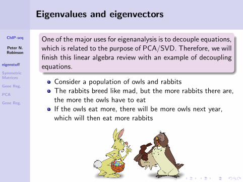
One of the major uses for eigenanalysis is to decouple equations,which is related to the purpose of PCA/SVD. Therefore, we willfinish this linear algebra review with an example of decouplingequations.
Consider a population of owls and rabbitsThe rabbits breed like mad, but the more rabbits there are,the more the owls have to eatIf the owls eat more, there will be more owls next year,which will then eat more rabbits
ChIP-seq
Peter N.Robinson
eigenstuff
SymmetricMatrices
Gene Reg.
PCA
Gene Reg.
Eigenvalues and eigenvectors
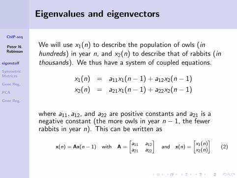
We will use x1(n) to describe the population of owls (inhundreds) in year n, and x2(n) to describe that of rabbits (inthousands). We thus have a system of coupled equations.
x1(n) = a11x1(n − 1) + a12x2(n − 1)
x2(n) = a21x1(n − 1) + a22x2(n − 1)
where a11, a12, and a22 are positive constants and a21 is anegative constant (the more owls in year n − 1, the fewerrabbits in year n). This can be written as
x(n) = Ax(n − 1) with A =
[a11 a12
a21 a22
]and x(n) =
[x1(n)x2(n)
](2)
ChIP-seq
Peter N.Robinson
eigenstuff
SymmetricMatrices
Gene Reg.
PCA
Gene Reg.
Eigenvalues and eigenvectors
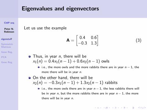
Let us use the example
A =
[0.4 0.6−0.3 1.3
](3)
Thus, in year n, there will bex1(n) = 0.4x1(n − 1) + 0.6x2(n − 1) owls
i.e., the more owls and the more rabbits there are in year n − 1, the
more there will be in year n.
On the other hand, there will bex2(n) = −0.3x1(n − 1) + 1.3x2(n − 1) rabbits
i.e., the more owls there are in year n − 1, the less rabbits there will
be in year n, but the more rabbits there are in year n − 1, the more
there will be in year n.
ChIP-seq
Peter N.Robinson
eigenstuff
SymmetricMatrices
Gene Reg.
PCA
Gene Reg.
Eigenvalues and eigenvectors
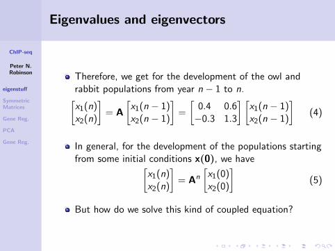
Therefore, we get for the development of the owl andrabbit populations from year n − 1 to n.[x1(n)x2(n)
]= A
[x1(n − 1)x2(n − 1)
]=
[0.4 0.6−0.3 1.3
] [x1(n − 1)x2(n − 1)
](4)
In general, for the development of the populations startingfrom some initial conditions x(0), we have[
x1(n)x2(n)
]= An
[x1(0)x2(0)
](5)
But how do we solve this kind of coupled equation?
ChIP-seq
Peter N.Robinson
eigenstuff
SymmetricMatrices
Gene Reg.
PCA
Gene Reg.
Eigenvalues and eigenvectors
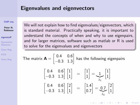
We will not explain how to find eigenvalues/eigenvectors, whichis standard material. Practically speaking, it is important tounderstand the concepts of when and why to use eigenpairs,and for larger matrices, software such as matlab or R is usedto solve for the eigenvalues and eigenvectors
The matrix A =
[0.4 0.6−0.3 1.3
]has the following eigenpairs
[0.4 0.6−0.3 1.3
] [11
]=
[11
]= 1︸︷︷︸
λ1
[11
][
0.4 0.6−0.3 1.3
] [21
]=
[1.40.7
]= 0.7︸︷︷︸
λ2
[21
]
ChIP-seq
Peter N.Robinson
eigenstuff
SymmetricMatrices
Gene Reg.
PCA
Gene Reg.
Eigenvalues and eigenvectors
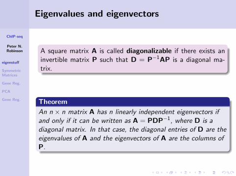
A square matrix A is called diagonalizable if there exists aninvertible matrix P such that D = P−1AP is a diagonal ma-trix.
Theorem
An n × n matrix A has n linearly independent eigenvectors ifand only if it can be written as A = PDP−1, where D is adiagonal matrix. In that case, the diagonal entries of D are theeigenvalues of A and the eigenvectors of A are the columns ofP.
ChIP-seq
Peter N.Robinson
eigenstuff
SymmetricMatrices
Gene Reg.
PCA
Gene Reg.
Eigenvalues and eigenvectors
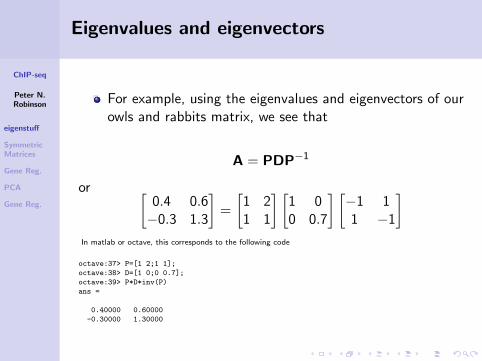
For example, using the eigenvalues and eigenvectors of ourowls and rabbits matrix, we see that
A = PDP−1
or [0.4 0.6−0.3 1.3
]=
[1 21 1
] [1 00 0.7
] [−1 11 −1
]In matlab or octave, this corresponds to the following code
octave:37> P=[1 2;1 1];
octave:38> D=[1 0;0 0.7];
octave:39> P*D*inv(P)
ans =
0.40000 0.60000
-0.30000 1.30000
ChIP-seq
Peter N.Robinson
eigenstuff
SymmetricMatrices
Gene Reg.
PCA
Gene Reg.
Eigenvalues and eigenvectors
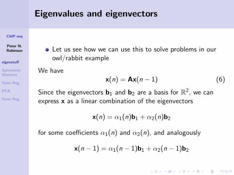
Let us see how we can use this to solve problems in ourowl/rabbit example
We havex(n) = Ax(n − 1) (6)
Since the eigenvectors b1 and b2 are a basis for R2, we canexpress x as a linear combination of the eigenvectors
x(n) = α1(n)b1 + α2(n)b2
for some coefficients α1(n) and α2(n), and analogously
x(n − 1) = α1(n − 1)b1 + α2(n − 1)b2
ChIP-seq
Peter N.Robinson
eigenstuff
SymmetricMatrices
Gene Reg.
PCA
Gene Reg.
Eigenvalues and eigenvectors
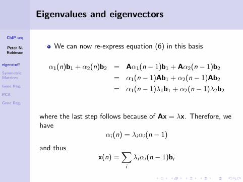
We can now re-express equation (6) in this basis
α1(n)b1 + α2(n)b2 = Aα1(n − 1)b1 + Aα2(n − 1)b2
= α1(n − 1)Ab1 + α2(n − 1)Ab2
= α1(n − 1)λ1b1 + α2(n − 1)λ2b2
where the last step follows because of Ax = λx. Therefore, wehave
αi (n) = λiαi (n − 1)
and thusx(n) =
∑i
λiαi (n − 1)bi
ChIP-seq
Peter N.Robinson
eigenstuff
SymmetricMatrices
Gene Reg.
PCA
Gene Reg.
Eigenvalues and eigenvectors
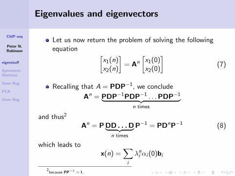
Let us now return the problem of solving the followingequation [
x1(n)x2(n)
]= An
[x1(0)x2(0)
](7)
Recalling that A = PDP−1, we conclude
An = PDP−1PDP−1 . . .PDP−1︸ ︷︷ ︸n times
and thus2
An = P DD . . .D︸ ︷︷ ︸n times
P−1 = PDnP−1 (8)
which leads tox(n) =
∑i
λni αi (0)bi
2because PP−1 = I.
ChIP-seq
Peter N.Robinson
eigenstuff
SymmetricMatrices
Gene Reg.
PCA
Gene Reg.
Eigenvalues and eigenvectors
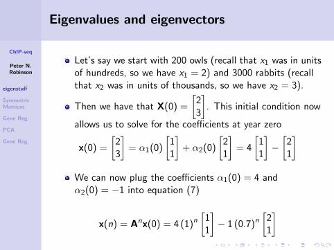
Let’s say we start with 200 owls (recall that x1 was in unitsof hundreds, so we have x1 = 2) and 3000 rabbits (recallthat x2 was in units of thousands, so we have x2 = 3).
Then we have that X(0) =
[23
]. This initial condition now
allows us to solve for the coefficients at year zero
x(0) =
[23
]= α1(0)
[11
]+ α2(0)
[21
]= 4
[11
]−[
21
]We can now plug the coefficients α1(0) = 4 andα2(0) = −1 into equation (7)
x(n) = Anx(0) = 4 (1)n[
11
]− 1 (0.7)n
[21
]
ChIP-seq
Peter N.Robinson
eigenstuff
SymmetricMatrices
Gene Reg.
PCA
Gene Reg.
Eigenvalues and eigenvectors
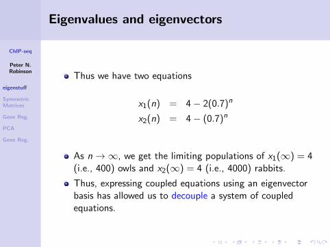
Thus we have two equations
x1(n) = 4− 2(0.7)n
x2(n) = 4− (0.7)n
As n→∞, we get the limiting populations of x1(∞) = 4(i.e., 400) owls and x2(∞) = 4 (i.e., 4000) rabbits.
Thus, expressing coupled equations using an eigenvectorbasis has allowed us to decouple a system of coupledequations.

ChIP-seq
Peter N.Robinson
eigenstuff
SymmetricMatrices
Gene Reg.
PCA
Gene Reg.
Outline
1 Eigenvalues and Eigenvectors
2 Symmetric Matrices
3 Back to Gene Regulation
4 Principle Component Analysis (PCA)
5 Getting back again to gene regulation
ChIP-seq
Peter N.Robinson
eigenstuff
SymmetricMatrices
Gene Reg.
PCA
Gene Reg.
Symmetric real matrices
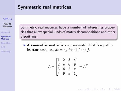
Symmetric real matrices have a number of interesting proper-ties that allow special kinds of matrix decompositions and otheralgorithms
A symmetric matrix is a square matrix that is equal toits transpose, i.e., aij = aji for all i and j .
A =
1 2 3 42 e 6 93 6 2 π4 9 π 1
= AT
ChIP-seq
Peter N.Robinson
eigenstuff
SymmetricMatrices
Gene Reg.
PCA
Gene Reg.
Orthogonal matrices
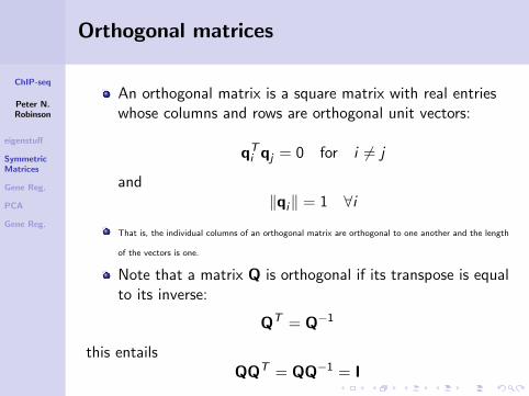
An orthogonal matrix is a square matrix with real entrieswhose columns and rows are orthogonal unit vectors:
qTi qj = 0 for i 6= j
and‖qi‖ = 1 ∀i
That is, the individual columns of an orthogonal matrix are orthogonal to one another and the length
of the vectors is one.
Note that a matrix Q is orthogonal if its transpose is equalto its inverse:
QT = Q−1
this entailsQQT = QQ−1 = I
ChIP-seq
Peter N.Robinson
eigenstuff
SymmetricMatrices
Gene Reg.
PCA
Gene Reg.
Spectral theorem
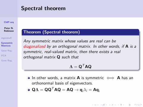
Theorem (Spectral theorem)
Any symmetric matrix whose values are real can bediagonalized by an orthogonal matrix. In other words, if A is asymmetric, real-valued matrix, then there exists a realorthogonal matrix Q such that
Λ = QTAQ
In other words, a matrix A is symmetric ⇐⇒ A has anorthonormal basis of eigenvectors.
QΛ = QQTAQ = AQ→ qiλi = Aqi
ChIP-seq
Peter N.Robinson
eigenstuff
SymmetricMatrices
Gene Reg.
PCA
Gene Reg.
Matrix Decompositions
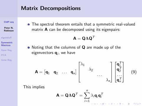
The spectral theorem entails that a symmetric real-valuedmatrix A can be decomposed using its eigenpairs:
A = QΛQT
Noting that the columns of Q are made up of theeigenvectors qi , we have
A =[q1 q2 . . . qn
] λ1
λ2
. . .λn
qT1
qT2
. . .qTn
(9)
This implies
A = QΛQT =n∑
i=1
λiqiqTi

ChIP-seq
Peter N.Robinson
eigenstuff
SymmetricMatrices
Gene Reg.
PCA
Gene Reg.
Outline
1 Eigenvalues and Eigenvectors
2 Symmetric Matrices
3 Back to Gene Regulation
4 Principle Component Analysis (PCA)
5 Getting back again to gene regulation
ChIP-seq
Peter N.Robinson
eigenstuff
SymmetricMatrices
Gene Reg.
PCA
Gene Reg.
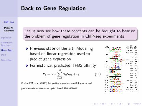
Back to Gene Regulation
Let us now see how these concepts can be brought to bear onthe problem of gene regulation in ChIP-seq experiments
Previous state of the art: Modelingbased on linear regression used topredict gene expression
For instance, predicted TFBS affinity
Yg = α+M∑
m=1
βmSmg + εg (10)
Conlon EM et al. (2003) Integrating regulatory motif discovery and
genome-wide expression analysis. PNAS 100:3339–44.
ChIP-seq
Peter N.Robinson
eigenstuff
SymmetricMatrices
Gene Reg.
PCA
Gene Reg.
Predicting Gene Regulation
However, thus far, the fraction of variation in gene expression(R2) explained by TF binding has been very moderate, varyingbetween 9.6% and 36.9% on various datasets from yeast tohuman
Potential reasons include
Insufficient data
suboptimal models
both.
The authors of Ouyang et al propose a new way to extract suitable features from
the ChIP-Seq data to serve as explanatory variables in the modeling of gene
expression. Additionally, they use SVD/PCA to better model divergent regulatory
effects of a TF that may be due to differences in the binding of cofactors and/or
the chromatin context.
ChIP-seq
Peter N.Robinson
eigenstuff
SymmetricMatrices
Gene Reg.
PCA
Gene Reg.
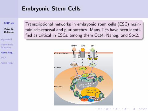
Embryonic Stem Cells
Transcriptional networks in embryonic stem cells (ESC) main-tain self-renewal and pluripotency. Many TFs have been identi-fied as critical in ESCs, among them Oct4, Nanog, and Sox2.
ChIP-seq
Peter N.Robinson
eigenstuff
SymmetricMatrices
Gene Reg.
PCA
Gene Reg.
Embryonic Stem Cells
A quantitative dissection of the functional roles of ESC regu-lators such as Oct4, Nanog, and Sox2 is still lacking.
Goal of experiment: Use ChIP-seq data from 12 ESCfactors3 and RNA-seq data to perform an analysis ofgenome-wide gene expression and TF binding data inESCs.
3Smad1, Stat3, Sox2, Oct4, Nanog, Esrrb, Tcfcp2l1, Klf4, Zfx, E2f1, Myc,and Mycn
ChIP-seq
Peter N.Robinson
eigenstuff
SymmetricMatrices
Gene Reg.
PCA
Gene Reg.
Transcription Factor Association Strength(TFAS)
Definition (Transcription Factor Association Strength)
The TFAS is a non-observable quantity that reflects the degreeto which a transcription factor binds to the regulatorysequences of a gene and thereby stimulates gene expression
There are innumerable definitions of TFAS or analogousquantities in the literature
The set of TFAS of all TFs for all Genes can be used forexample in network inference algorithms
ChIP-seq
Peter N.Robinson
eigenstuff
SymmetricMatrices
Gene Reg.
PCA
Gene Reg.
Binary TFAS
Traditionally, a TF binding peak is usually associated with thenearest gene (uslly based on the distance between the midpointof the peak and the transcription start site (TSS).
Denoting the binary TFAS as aij , then aij = 1 if gene i isassociated with a ChIP-seq peak of TF j ; otherwiseaij = 0.
A binary TFAS is easy to calculate
The binary TFAS approach does not take into account theintensity of the peaks and the relative distance betweenpeaks and genes.
ChIP-seq
Peter N.Robinson
eigenstuff
SymmetricMatrices
Gene Reg.
PCA
Gene Reg.
Continuous TFAS
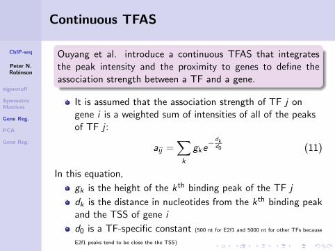
Ouyang et al. introduce a continuous TFAS that integratesthe peak intensity and the proximity to genes to define theassociation strength between a TF and a gene.
It is assumed that the association strength of TF j ongene i is a weighted sum of intensities of all of the peaksof TF j :
aij =∑k
gke− dk
d0 (11)
In this equation,
gk is the height of the kth binding peak of the TF j
dk is the distance in nucleotides from the kth binding peakand the TSS of gene i
d0 is a TF-specific constant (500 nt for E2f1 and 5000 nt for other TFs because
E2f1 peaks tend to be close the the TSS)
ChIP-seq
Peter N.Robinson
eigenstuff
SymmetricMatrices
Gene Reg.
PCA
Gene Reg.
Continuous TFAS
When dkd0
is very large the contribution of the peak will beeffectively zero.
Therefore, the summation is taken over peaks that are nottoo far away from the TSS (e.g., ≤ 1× 10⁶ nucleotides)
The TFAS values are then log-transformed4 and quantilenormalized5
For N genes and M TFs, the TFAS profiles are stored inan N ×M matrix A.
4i.e., a
′ij = log aij
5i.e., the a
′ij are sorted; then, the same number of samples from the reference distribution
(e.g., Gaussian) are taken from the cumulative distribution function, and the a′ij are assigned
the values of the reference distribution.
ChIP-seq
Peter N.Robinson
eigenstuff
SymmetricMatrices
Gene Reg.
PCA
Gene Reg.
Continuous TFAS
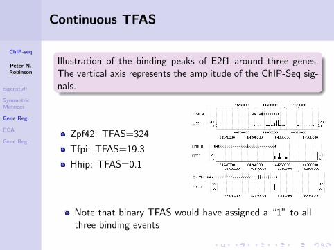
Illustration of the binding peaks of E2f1 around three genes.The vertical axis represents the amplitude of the ChIP-Seq sig-nals.
Zpf42: TFAS=324
Tfpi: TFAS=19.3
Hhip: TFAS=0.1
Note that binary TFAS would have assigned a “1” to allthree binding events
ChIP-seq
Peter N.Robinson
eigenstuff
SymmetricMatrices
Gene Reg.
PCA
Gene Reg.
Continuous TFAS
The continuous TFAS was the first major new idea of thepaper.
The authors now validate the utility of continuous TFASby comparing its performance to that of binary TFAS
They use a principle-components analysis (PCA)regression model to compare the ability of the bindingpeaks of the 12 ESC transcription factors with respect totheir ability to predict the expression of genes in ESCs (asmeasured by RNA-seq).
By examining the quality of the respective regressionmodels, we can determine which method performed best
To understand this, we will have to review PCA, and howall of this is used to perform regression.

ChIP-seq
Peter N.Robinson
eigenstuff
SymmetricMatrices
Gene Reg.
PCA
Gene Reg.
Outline
1 Eigenvalues and Eigenvectors
2 Symmetric Matrices
3 Back to Gene Regulation
4 Principle Component Analysis (PCA)
5 Getting back again to gene regulation
ChIP-seq
Peter N.Robinson
eigenstuff
SymmetricMatrices
Gene Reg.
PCA
Gene Reg.
PCA: Intuition, Goals, Algorithm
We will now present an explanation of the PCA algorithm thatis closely based on the document A Tutorial on Principal Com-ponent Analysis by Jonathon Shlensa
aAvailable at http://www.snl.salk.edu/ shlens/
PCA uses an orthogonal transformation to convert a set ofobservations of possibly correlated variables into a set ofvalues of linearly uncorrelated variables called principalcomponents (PC). The first PC accounts for as much ofthe variability in the data as possible, and each succeedingPC accounts for as much of the remaining variability aspossible.
An extremely important tool in the repertoire ofalgorithms for data analysis in bioinformatics
ChIP-seq
Peter N.Robinson
eigenstuff
SymmetricMatrices
Gene Reg.
PCA
Gene Reg.
PCA: Intuition, Goals, Algorithm
A common problem in bioinformatics
We are trying to understand a complicated biologicalexperiment with lots of genomics data that comes frommultiple sources (e.g., ChIP-seq from 12 TFs, RNA-seq data),is noisy, and is partially redundant
We want to understand the essential patterns in the data
We will demonstrate this using a slightly simpler example,and then explain the relevance to the ESC experiment

ChIP-seq
Peter N.Robinson
eigenstuff
SymmetricMatrices
Gene Reg.
PCA
Gene Reg.
The clueless physicist
Let us imagine we are studying the motion of an ideal spring,consisting of a ball attached to a massless, frictionless spring.The ball is released a small distance away from equilibrium;because it is an ideal spring, it should oscillate indefinitely alongits axis of motion.

ChIP-seq
Peter N.Robinson
eigenstuff
SymmetricMatrices
Gene Reg.
PCA
Gene Reg.
The clueless physicist
Graphic: Jonathon Shlens
Let’s say we want to determine the motion of the spring asa function of time
We therefore place three movie cameras around the springand record images at 120 Hz
ChIP-seq
Peter N.Robinson
eigenstuff
SymmetricMatrices
Gene Reg.
PCA
Gene Reg.
The clueless physicist
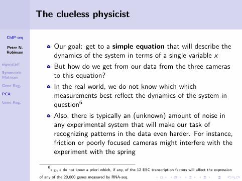
Our goal: get to a simple equation that will describe thedynamics of the system in terms of a single variable x
But how do we get from our data from the three camerasto this equation?
In the real world, we do not know which whichmeasurements best reflect the dynamics of the system inquestion6
Also, there is typically an (unknown) amount of noise inany experimental system that will make our task ofrecognizing patterns in the data even harder. For instance,friction or poorly focused cameras might interfere with theexperiment with the spring
6e.g., e do not know a priori which, if any, of the 12 ESC transcription factors will affect the expression
of any of the 20,000 genes measured by RNA-seq.
ChIP-seq
Peter N.Robinson
eigenstuff
SymmetricMatrices
Gene Reg.
PCA
Gene Reg.
The goals of PCA
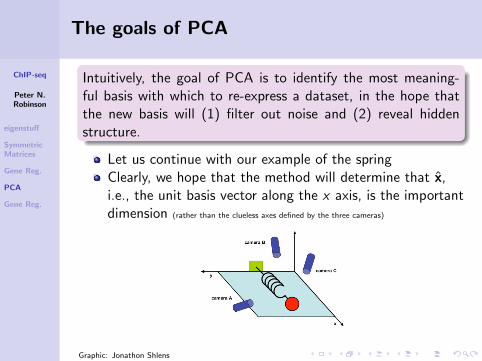
Intuitively, the goal of PCA is to identify the most meaning-ful basis with which to re-express a dataset, in the hope thatthe new basis will (1) filter out noise and (2) reveal hiddenstructure.
Let us continue with our example of the springClearly, we hope that the method will determine that x,i.e., the unit basis vector along the x axis, is the importantdimension (rather than the clueless axes defined by the three cameras)
Graphic: Jonathon Shlens
ChIP-seq
Peter N.Robinson
eigenstuff
SymmetricMatrices
Gene Reg.
PCA
Gene Reg.
The clueless physicist
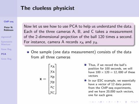
Now let us see how to use PCA to help us understand the data.Each of the three cameras A, B, and C takes a measurementof the 2-dimensional projection of the ball 120 times a second.For instance, camera A records xA and yA.
One sample (one data measurement) consists of the datafrom all three cameras
x =
xAyAxByBxCyC
Thus, if we record the ball’sposition for 100 seconds, we willhave 100× 120 = 12, 000 of thesevectors
In our ESC example, we essentiallyhave a vector of 12 data pointsfrom the ChIP-seq experiments,and we have 20,000 such vectors,one for each gene.
ChIP-seq
Peter N.Robinson
eigenstuff
SymmetricMatrices
Gene Reg.
PCA
Gene Reg.
The naive basis
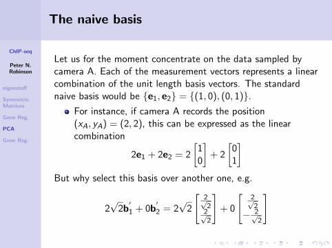
Let us for the moment concentrate on the data sampled bycamera A. Each of the measurement vectors represents a linearcombination of the unit length basis vectors. The standardnaive basis would be {e1, e2} = {(1, 0), (0, 1)}.
For instance, if camera A records the position(xA, yA) = (2, 2), this can be expressed as the linearcombination
2e1 + 2e2 = 2
[10
]+ 2
[01
]But why select this basis over another one, e.g.
2√
2b′1 + 0b
′2 = 2
√2
[2√2
2√2
]+ 0
[2√2
− 2√2
]
ChIP-seq
Peter N.Robinson
eigenstuff
SymmetricMatrices
Gene Reg.
PCA
Gene Reg.
The naive basis
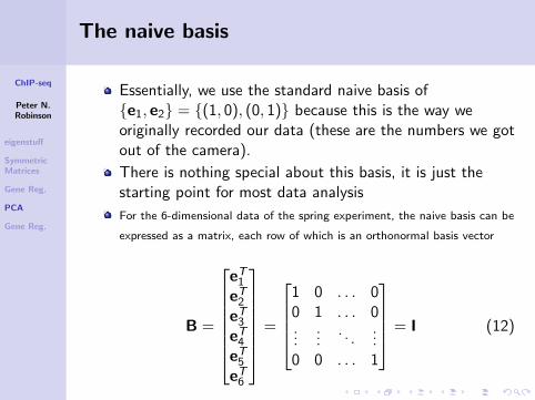
Essentially, we use the standard naive basis of{e1, e2} = {(1, 0), (0, 1)} because this is the way weoriginally recorded our data (these are the numbers we gotout of the camera).
There is nothing special about this basis, it is just thestarting point for most data analysis
For the 6-dimensional data of the spring experiment, the naive basis can be
expressed as a matrix, each row of which is an orthonormal basis vector
B =
eT1eT2eT3eT4eT5eT6
=
1 0 . . . 00 1 . . . 0...
.... . .
...0 0 . . . 1
= I (12)
ChIP-seq
Peter N.Robinson
eigenstuff
SymmetricMatrices
Gene Reg.
PCA
Gene Reg.
PCA: A more useful basis?
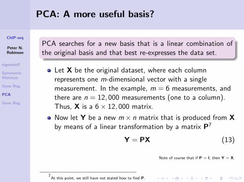
PCA searches for a new basis that is a linear combination ofthe original basis and that best re-expresses the data set.
Let X be the original dataset, where each columnrepresents one m-dimensional vector with a singlemeasurement. In the example, m = 6 measurements, andthere are n = 12, 000 measurements (one to a column).Thus, X is a 6× 12, 000 matrix.
Now let Y be a new m× n matrix that is produced from Xby means of a linear transformation by a matrix P7
Y = PX (13)
Note of course that if P = I, then Y = X.
7At this point, we still have not stated how to find P.
ChIP-seq
Peter N.Robinson
eigenstuff
SymmetricMatrices
Gene Reg.
PCA
Gene Reg.
PCA: A more useful basis?
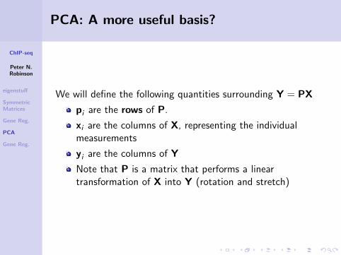
We will define the following quantities surrounding Y = PX
pi are the rows of P.
xi are the columns of X, representing the individualmeasurements
yi are the columns of Y
Note that P is a matrix that performs a lineartransformation of X into Y (rotation and stretch)
ChIP-seq
Peter N.Robinson
eigenstuff
SymmetricMatrices
Gene Reg.
PCA
Gene Reg.
PCA: A more useful basis?
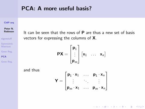
It can be seen that the rows of P are thus a new set of basisvectors for expressing the columns of X.
PX =
p1...
pm
[x1 . . . xn]
and thus
Y =
p1 · x1 . . . p1 · xn...
. . ....
pm · x1 . . . pm · xn
ChIP-seq
Peter N.Robinson
eigenstuff
SymmetricMatrices
Gene Reg.
PCA
Gene Reg.
PCA: A more useful basis?
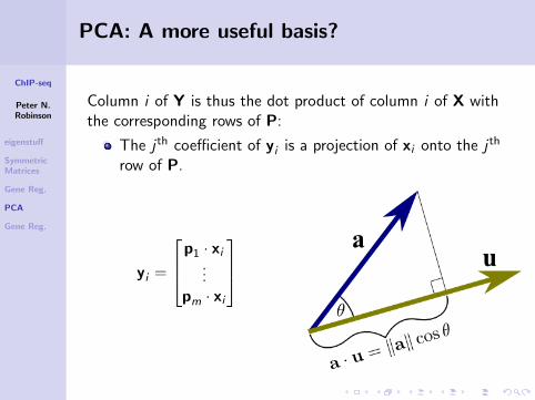
Column i of Y is thus the dot product of column i of X withthe corresponding rows of P:
The j th coefficient of yi is a projection of xi onto the j th
row of P.
yi =
p1 · xi...
pm · xi
ChIP-seq
Peter N.Robinson
eigenstuff
SymmetricMatrices
Gene Reg.
PCA
Gene Reg.
PCA: A more useful basis?
We have left out the question of how exactly to find the ma-trix P? The PCA procedures is based upon features that areconsidered desirable for the matrix Y to exhibit, which we willconsider next.
There are two essential topics
Noise
Redundancy
ChIP-seq
Peter N.Robinson
eigenstuff
SymmetricMatrices
Gene Reg.
PCA
Gene Reg.
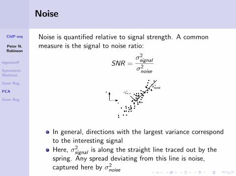
Noise
Noise is quantified relative to signal strength. A commonmeasure is the signal to noise ratio:
SNR =σ2signal
σ2noise
In general, directions with the largest variance correspondto the interesting signal
Here, σ2signal is along the straight line traced out by the
spring. Any spread deviating from this line is noise,captured here by σ2
noise
ChIP-seq
Peter N.Robinson
eigenstuff
SymmetricMatrices
Gene Reg.
PCA
Gene Reg.
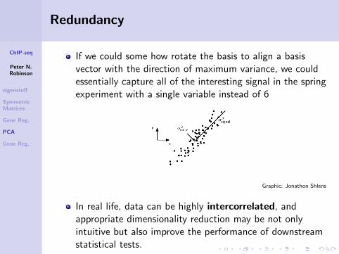
Redundancy
If we could some how rotate the basis to align a basisvector with the direction of maximum variance, we couldessentially capture all of the interesting signal in the springexperiment with a single variable instead of 6
Graphic: Jonathon Shlens
In real life, data can be highly intercorrelated, andappropriate dimensionality reduction may be not onlyintuitive but also improve the performance of downstreamstatistical tests.
ChIP-seq
Peter N.Robinson
eigenstuff
SymmetricMatrices
Gene Reg.
PCA
Gene Reg.
Covariance matrix
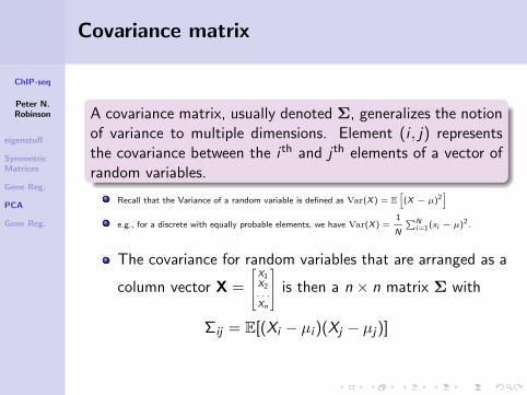
A covariance matrix, usually denoted Σ, generalizes the notionof variance to multiple dimensions. Element (i , j) representsthe covariance between the i th and j th elements of a vector ofrandom variables.
Recall that the Variance of a random variable is defined as Var(X ) = E[
(X − µ)2]
e.g., for a discrete with equally probable elements, we have Var(X ) =1
N
∑Ni=1(xi − µ)2.
The covariance for random variables that are arranged as a
column vector X =
X1X2. . .Xn
is then a n × n matrix Σ with
Σij = E[(Xi − µi )(Xj − µj)]
ChIP-seq
Peter N.Robinson
eigenstuff
SymmetricMatrices
Gene Reg.
PCA
Gene Reg.
Covariance matrix
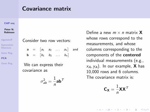
Consider two row vectors:
a =[a1 a2 . . . an
]and
b =[b1 b2 . . . bn
]We can express their
covariance as
σ2ab =
1
nabT
Define a new m × n matrix Xwhose rows correspond to themeasurements, and whosecolumns corresponding to thecomponents of the centeredindividual measurements (e.g.,xA, yA). In our example, X has10,000 rows and 6 columns.The covariance matrix is:
CX =1
nXXT
ChIP-seq
Peter N.Robinson
eigenstuff
SymmetricMatrices
Gene Reg.
PCA
Gene Reg.
Covariance matrix
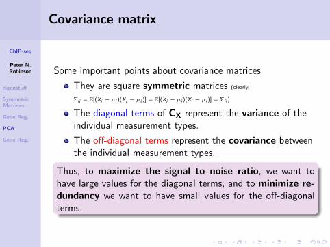
Some important points about covariance matrices
They are square symmetric matrices (clearly,
Σij = E[(Xi − µi )(Xj − µj )] = E[(Xj − µj )(Xi − µi )] = Σji )
The diagonal terms of CX represent the variance of theindividual measurement types.
The off-diagonal terms represent the covariance betweenthe individual measurement types.
Thus, to maximize the signal to noise ratio, we want tohave large values for the diagonal terms, and to minimize re-dundancy we want to have small values for the off-diagonalterms.
ChIP-seq
Peter N.Robinson
eigenstuff
SymmetricMatrices
Gene Reg.
PCA
Gene Reg.
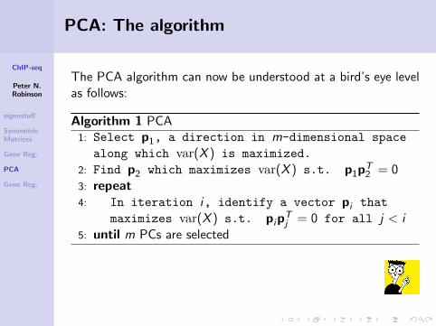
PCA: The algorithm
The PCA algorithm can now be understood at a bird’s eye levelas follows:
Algorithm 1 PCA1: Select p1, a direction in m-dimensional space
along which var(X ) is maximized.
2: Find p2 which maximizes var(X ) s.t. p1pT2 = 0
3: repeat4: In iteration i, identify a vector pi that
maximizes var(X ) s.t. pipTj = 0 for all j < i
5: until m PCs are selected
ChIP-seq
Peter N.Robinson
eigenstuff
SymmetricMatrices
Gene Reg.
PCA
Gene Reg.
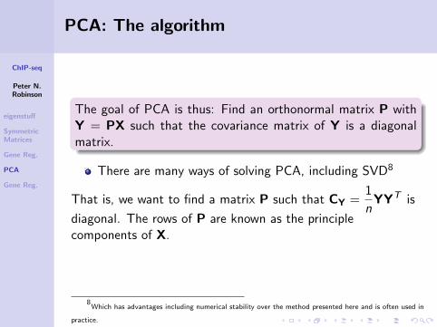
PCA: The algorithm
The goal of PCA is thus: Find an orthonormal matrix P withY = PX such that the covariance matrix of Y is a diagonalmatrix.
There are many ways of solving PCA, including SVD8
That is, we want to find a matrix P such that CY =1
nYYT is
diagonal. The rows of P are known as the principlecomponents of X.
8Which has advantages including numerical stability over the method presented here and is often used in
practice.
ChIP-seq
Peter N.Robinson
eigenstuff
SymmetricMatrices
Gene Reg.
PCA
Gene Reg.
PCA: The algorithm
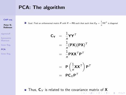
Goal: Find an orthonormal matrix P with Y = PX such that such that CY =1
nYYT is diagonal
CY =1
nYYT
=1
n(PX)(PX)T
=1
nPXXTPT
= P
(1
nXXT
)PT
= PCXPT
Thus, CY is related to the covariance matrix of X
ChIP-seq
Peter N.Robinson
eigenstuff
SymmetricMatrices
Gene Reg.
PCA
Gene Reg.
PCA: The algorithm
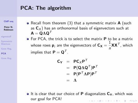
Recall from theorem (3) that a symmetric matrix A (suchas CX ) has an orthonormal basis of eigenvectors such atA = QΛQT
For PCA, the trick is to select the matrix P to be a matrix
whose rows pi are the eigenvectors of CX =1
nXXT , which
implies that P = QT .
CY = PCXPT
= P(QΛQT )PT
= P(PTΛP)PT
= Λ
It is clear that our choice of P diagonalizes CY, which wasour goal for PCA!
ChIP-seq
Peter N.Robinson
eigenstuff
SymmetricMatrices
Gene Reg.
PCA
Gene Reg.
PCA: The algorithm
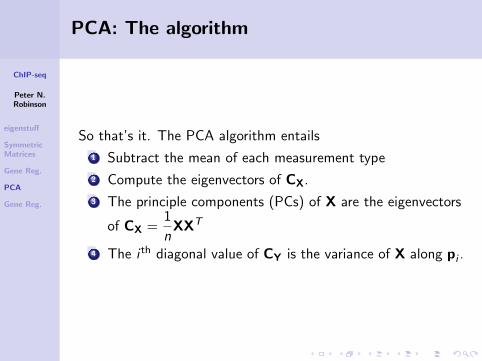
So that’s it. The PCA algorithm entails
1 Subtract the mean of each measurement type
2 Compute the eigenvectors of CX.
3 The principle components (PCs) of X are the eigenvectors
of CX =1
nXXT
4 The i th diagonal value of CY is the variance of X along pi .

ChIP-seq
Peter N.Robinson
eigenstuff
SymmetricMatrices
Gene Reg.
PCA
Gene Reg.
PCA: Application
To give intuition about the PCA, we will show how it is usedto examine and visualize a dataset about cars. Specificationsare given for 428 new vehicles for the 2004 year. The variablesrecorded include price, measurements relating to the size of thevehicle, and fuel efficiency.
Suggested Retail Price
Dealer Cost
Engine Size
Number of Cylinders
Horsepower
City Miles Per Gallon
Highway Miles Per Gallon
Weight (Pounds)
Wheel Base (inches)
Length (inches)
Width (inches)
ChIP-seq
Peter N.Robinson
eigenstuff
SymmetricMatrices
Gene Reg.
PCA
Gene Reg.
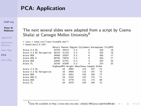
PCA: Application
The next several slides were adapted from a script by CosmaShalizi at Carnegie Mellon University9
> cars = read.csv("cars-fixed04.dat")
> head(cars[,8:18])
Retail Dealer Engine Cylinders Horsepower CityMPG
Acura 3.5 RL 43755 39014 3.5 6 225 18
Acura 3.5 RL Navigation 46100 41100 3.5 6 225 18
Acura MDX 36945 33337 3.5 6 265 17
Acura NSX S 89765 79978 3.2 6 290 17
Acura RSX 23820 21761 2.0 4 200 24
Acura TL 33195 30299 3.2 6 270 20
HighwayMPG Weight Wheelbase Length Width
Acura 3.5 RL 24 3880 115 197 72
Acura 3.5 RL Navigation 24 3893 115 197 72
Acura MDX 23 4451 106 189 77
Acura NSX S 24 3153 100 174 71
Acura RSX 31 2778 101 172 68
Acura TL 28 3575 108 186 72
9Data file available at http://www.stat.cmu.edu/ cshalizi/490/pca/cars-fixed04.dat

ChIP-seq
Peter N.Robinson
eigenstuff
SymmetricMatrices
Gene Reg.
PCA
Gene Reg.
PCA: Application
There are complex correlations between different attributes of the cars. (Red: highly correlated, blue: so-so,
yellow: low correlation)
ChIP-seq
Peter N.Robinson
eigenstuff
SymmetricMatrices
Gene Reg.
PCA
Gene Reg.
PCA: Application
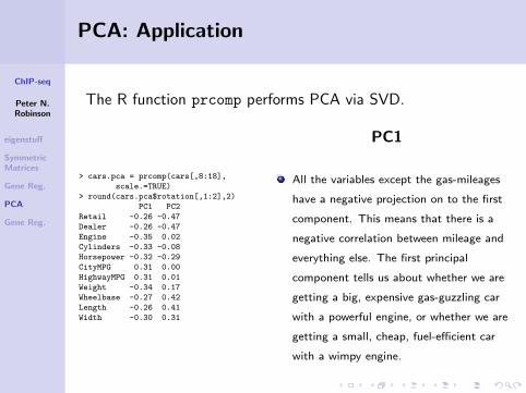
The R function prcomp performs PCA via SVD.
> cars.pca = prcomp(cars[,8:18],
scale.=TRUE)
> round(cars.pca$rotation[,1:2],2)
PC1 PC2
Retail -0.26 -0.47
Dealer -0.26 -0.47
Engine -0.35 0.02
Cylinders -0.33 -0.08
Horsepower -0.32 -0.29
CityMPG 0.31 0.00
HighwayMPG 0.31 0.01
Weight -0.34 0.17
Wheelbase -0.27 0.42
Length -0.26 0.41
Width -0.30 0.31
PC1
All the variables except the gas-mileages
have a negative projection on to the first
component. This means that there is a
negative correlation between mileage and
everything else. The first principal
component tells us about whether we are
getting a big, expensive gas-guzzling car
with a powerful engine, or whether we are
getting a small, cheap, fuel-efficient car
with a wimpy engine.

ChIP-seq
Peter N.Robinson
eigenstuff
SymmetricMatrices
Gene Reg.
PCA
Gene Reg.
PCA: Application
> round(cars.pca$rotation[,1:2],2)
PC1 PC2
Retail -0.26 -0.47
Dealer -0.26 -0.47
Engine -0.35 0.02
Cylinders -0.33 -0.08
Horsepower -0.32 -0.29
CityMPG 0.31 0.00
HighwayMPG 0.31 0.01
Weight -0.34 0.17
Wheelbase -0.27 0.42
Length -0.26 0.41
Width -0.30 0.31
Note: MPG=miles per gallon
PC2
Engine size and gas mileage hardly project
on to PC2 at all. Instead we have a
contrast between the physical size of the
car (positive projection) and the price and
horsepower. This axis separates mini-vans,
trucks and SUVs (big, not so expensive,
not so much horse-power) from sports-cars
(small, expensive, lots of horse-power).

ChIP-seq
Peter N.Robinson
eigenstuff
SymmetricMatrices
Gene Reg.
PCA
Gene Reg.
PCA: Application
Loadings Plot for PC1
Variable Loadings
Engine
Weight
Cylinders
Horsepower
Width
Wheelbase
Retail
Dealer
Length
HighwayMPG
CityMPG
−0.2 0.0 0.2
●
●
●
●
●
●
●
●
●
●
●
Loadings Plot for PC2
Variable Loadings
Dealer
Retail
Horsepower
Cylinders
CityMPG
HighwayMPG
Engine
Weight
Width
Length
Wheelbase
−0.4 −0.2 0.0 0.2 0.4
●
●
●
●
●
●
●
●
●
●
●
The elements of an eigenvector are the weights pij , andare also known as loadings10.
The figures show the loadings of p1 and p2, i.e., the coefficients representing the linear combinations
of the original variables to together make up the eigenvectors
10loadings are called rotations in some texts
ChIP-seq
Peter N.Robinson
eigenstuff
SymmetricMatrices
Gene Reg.
PCA
Gene Reg.
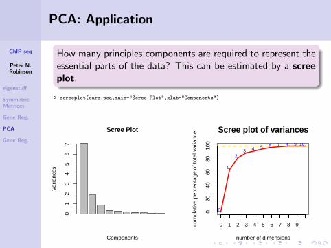
PCA: Application
How many principles components are required to represent theessential parts of the data? This can be estimated by a screeplot.
> screeplot(cars.pca,main="Scree Plot",xlab="Components")
Scree Plot
Components
Var
ianc
es
01
23
45
67
Scree plot of variances
number of dimensions
cum
ulat
ive
perc
enta
ge o
f tot
al v
aria
nce
0 1 2 3 4 5 6 7 8 9
020
4060
8010
00
1
23 4 5 6 7 8 9 10
ChIP-seq
Peter N.Robinson
eigenstuff
SymmetricMatrices
Gene Reg.
PCA
Gene Reg.
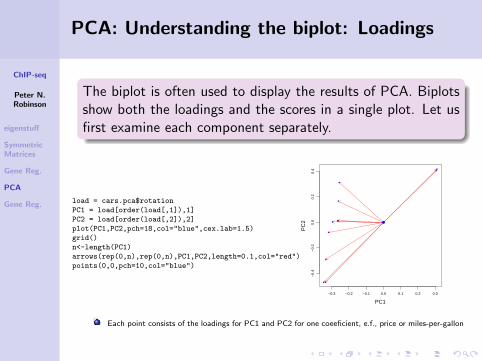
PCA: Understanding the biplot: Loadings
The biplot is often used to display the results of PCA. Biplotsshow both the loadings and the scores in a single plot. Let usfirst examine each component separately.
load = cars.pca$rotation
PC1 = load[order(load[,1]),1]
PC2 = load[order(load[,2]),2]
plot(PC1,PC2,pch=18,col="blue",cex.lab=1.5)
grid()
n<-length(PC1)
arrows(rep(0,n),rep(0,n),PC1,PC2,length=0.1,col="red")
points(0,0,pch=10,col="blue")
−0.3 −0.2 −0.1 0.0 0.1 0.2 0.3
−0.
4−
0.2
0.0
0.2
0.4
PC1P
C2 ●
Each point consists of the loadings for PC1 and PC2 for one coeeficient, e.f., price or miles-per-gallon
ChIP-seq
Peter N.Robinson
eigenstuff
SymmetricMatrices
Gene Reg.
PCA
Gene Reg.
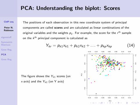
PCA: Understanding the biplot: Scores
The positions of each observation in this new coordinate system of principal
components are called scores and are calculated as linear combinations of the
original variables and the weights pij . For example, the score for the r th sample
on the kth principal component is calculated as
Ykr = pk1xk1 + pk2xk2 + . . .+ pkpxkp (14)
The figure shows the Yk1 scores (on
x-axis) and the Yk2 (on Y axis)
●●●
●
●
● ● ●●
●
●●●●
●
●●●
●
●
●●
●
●●
●
●●●
●●
●●
●●
●
●
●●●
●●
●
●
●
●
●●
●●
●
● ●●●
●●
●
●
●●
●
●
●
●
●●●
●
●
●●
● ●
●●
●
●●
●
●
●
●●
●●
●●
●
●
●
●
●
●
●
●●
●
●●
●●
●●
●●
●●
●●
●
●
●
●
●●
●
●●●
●
●
●
●●●
●
●
●●
●
●
●
●●
●● ●●
●
●●●
●
●●
●
●
●
●●●
●●●●
●●
●
●●●
●●●●●
●●
●
●●
●
●
●
●●●
●
●●
●●
●●
●
●
●
●●●
●
●
●●●
● ●
●
●●
●
●
●●●●
●
●
●
●
●●
●●
●
●●
●
●●
●●
●
●
●●●●
●
●
●
●
●
●
●
●●
●●
●
●●
●
●
●
●
●
●
●●●
●
●
●
●●●
●●
●
●●
●●
●
●
●
●●
●
●●●●
●
●
●
●
●●●
●●
●
●
●
●
●
●●●
●
●●●
●● ●
●
●
●
●
●●
●
●
●●
●●●●●
●●
●
●●
●●
●
●
●●●
●
●●●●
●
●●
●
●
●●●
●
●
●●
●
●●
●
●●●
●● ●
●
●●
●
●
●
●●
●
●●
●
●
●
●●
●●
●
●●
●
●●
●
●
●
●
●●
● ●
●●
−0.15 −0.10 −0.05 0.00 0.05 0.10 0.15
−0.
3−
0.2
−0.
10.
00.
1
PC1
PC
2
−0.15 −0.10 −0.05 0.00 0.05 0.10 0.15
−0.
3−
0.2
−0.
10.
00.
1
ChIP-seq
Peter N.Robinson
eigenstuff
SymmetricMatrices
Gene Reg.
PCA
Gene Reg.
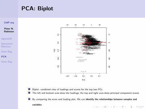
PCA: Biplot
Biplot: combined view of loadings and scores for the top two PCs
The left and bottom axes show the loadings; the top and right axes show principal component scores.
By comparing the score and loading plot, We can identify the relationships between samples and
variables

ChIP-seq
Peter N.Robinson
eigenstuff
SymmetricMatrices
Gene Reg.
PCA
Gene Reg.
Outline
1 Eigenvalues and Eigenvectors
2 Symmetric Matrices
3 Back to Gene Regulation
4 Principle Component Analysis (PCA)
5 Getting back again to gene regulation
ChIP-seq
Peter N.Robinson
eigenstuff
SymmetricMatrices
Gene Reg.
PCA
Gene Reg.
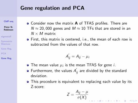
Gene regulation and PCA
Consider now the matrix A of TFAS profiles. There areN ≈ 20, 000 genes and M ≈ 10 TFs that are stored in anN ×M matrix
First, this matrix is centered, i.e., the mean of each row issubtracted from the values of that row.
A′ij = Aij − µi
The mean value µi is the mean TFAS for gene i .
Furthermore, the values A′ij are divided by the standard
deviation.
This procedure is equivalent to replacing each value by itsZ-score:
Z =Aij − µσ(X )
ChIP-seq
Peter N.Robinson
eigenstuff
SymmetricMatrices
Gene Reg.
PCA
Gene Reg.
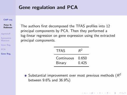
Gene regulation and PCA
The authors first decomposed the TFAS profiles into 12principal components by PCA. Then they performed alog-linear regression on gene expression using the extractedprincipal components.
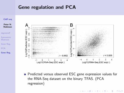
TFAS R2
Continuous 0.650Binary 0.425
Substantial improvement over most previous methods (R2
between 9.6% and 36.9%)
ChIP-seq
Peter N.Robinson
eigenstuff
SymmetricMatrices
Gene Reg.
PCA
Gene Reg.
Gene regulation and PCA
Predicted versus observed ESC gene expression values forthe RNA-Seq dataset on the binary TFAS. (PCAregression)
ChIP-seq
Peter N.Robinson
eigenstuff
SymmetricMatrices
Gene Reg.
PCA
Gene Reg.
Gene regulation and PCA
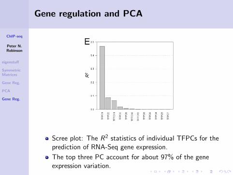
Scree plot: The R2 statistics of individual TFPCs for theprediction of RNA-Seq gene expression.
The top three PC account for about 97% of the geneexpression variation.
ChIP-seq
Peter N.Robinson
eigenstuff
SymmetricMatrices
Gene Reg.
PCA
Gene Reg.
Gene regulation and PCA
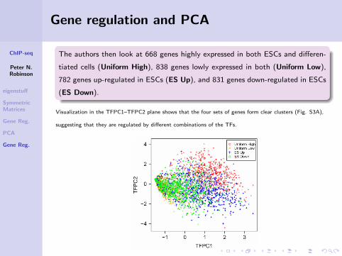
The authors then look at 668 genes highly expressed in both ESCs and differen-
tiated cells (Uniform High), 838 genes lowly expressed in both (Uniform Low),
782 genes up-regulated in ESCs (ES Up), and 831 genes down-regulated in ESCs
(ES Down).
Visualization in the TFPC1–TFPC2 plane shows that the four sets of genes form clear clusters (Fig. S3A),
suggesting that they are regulated by different combinations of the TFs.
ChIP-seq
Peter N.Robinson
eigenstuff
SymmetricMatrices
Gene Reg.
PCA
Gene Reg.
Gene regulation and PCA
Finally, The authors claimed to learn regulatory rules thatare combinations of TFPCs.
For example, the Uniform Low gene set can be determinedby TFPC1 < −0.77 (score of a gene) ANDTFPC2 < 0.25
The paper rewards more close reading, but let us stophere.
In sum, joint modeling of ChIP-Seq and gene expressiondata (RNA- Seq and microarray) was used to quantify thecontribution of TF binding on gene expression regulation.
PCA was used to capture signal within noisy and partiallyredundant data
Interpretation of the patterns of the PC loadings offerssome insight into the gene regulation of ESCs

ChIP-seq
Peter N.Robinson
eigenstuff
SymmetricMatrices
Gene Reg.
PCA
Gene Reg.
The End of the Lecture as We Know It
Email:[email protected]
Office hours byappointment
Lectures were once useful; but now, when all can read, and booksare so numerous, lectures are unnecessary. If your attention fails,and you miss a part of a lecture, it is lost; you cannot go back as
you do upon a book... People have nowadays got a strangeopinion that everything should be taught by lectures. Now, Icannot see that lectures can do as much good as reading thebooks from which the lectures are taken. I know nothing that
can be best taught by lectures, except where experiments are tobe shown. You may teach chymistry by lectures. You might
teach making shoes by lectures!
Samuel Johnson, quoted in Boswell’s Life of Johnson (1791).