1

Chinese Happiness Index and Its

Influencing Factors Analysis

ZIMU HU

Master of Science Thesis

Stockholm, Sweden 2012

2

Chinese Happiness Index and Its

Influencing Factors Analysis

Zimu Hu

Master of Science Thesis INDEK 2012:19

KTH Industrial Engineering and Management

SE-100 44 STOCKHOLM

3

Master of Science Thesis INDEK 2012:19

Chinese Happiness Index and Its Influencing Factors Analysis

Zimu Hu

Approved

2012-04-05

Examiner

Kristina Nyström

Supervisor

Per Thulin

Abstract

In recent decades, economists are gradually showing their interests in the

study of happiness. They even put forward some challenges to the traditional

theories. In contrast, studies on Chinese happiness problem are not enough in terms of

breadth and depth.

This paper used the data provided by China General Social Survey to conduct an

empirical analysis. The model author adopted is Ordered Discrete Choice model. In

the empirical section, author analyzed the impact of income, macroeconomic

variables, etc.

Ultimately, based on the empirical results, author proposed some policy

recommendations and further study suggestions.

Key-words: Happiness, Influencing Factors, Ordered discrete choice model, Easterlin

Paradox, Policy Recommendation

4

Acknowledge First of all, I would like to express my deepest gratitude to my supervisor Per

Thulin, whose patience and constantly suggestions stimulated me during the entire

period of writing my thesis. I will always remember such a respectful teacher

throughout my life.

I would also like to thank Hans Lööf, Kristina Nyström, and all the other staff of the

Department of Economics at KTH.

In addition, I want to show my great appreciation to "Chinese General Social Survey",

who offered the valuable data to this paper.

Last but not least, a special thank goes to my family for their support and

encouragement all the time.

5

Content 1. Introduction·························································································06

1.1 Purposes of this paper··························································06

1.2 Background·······································································06

1.3 Structure of this paper··························································07

2. Literature Review ················································································08 2.1 Previous Studies··································································08

2.2 Researches of happiness in China··············································11

3. Theoretical analysis·············································································13 3.1 Definition of happiness·························································13

3.2 Happiness from economic perspective·······································13

4. Data and model description·································································17 4.1 Data sources······································································17

4.2 Variable Description·····························································18

4.2.1 Definition and its Descriptive statistics····································18

4.2.2 Test for multicollinearity·····················································20

4.3 Ordered discrete choice model (Ordered Logit model) ····················21

4.4 Specific format of discrete choice model in this paper······················23

5. Empirical analysis·················································································25

5.1 Basic regression results·························································25

5.2 Introduce income2 into the model············································27

5.3 Introduce relative income into the model···································30

5.4 The impact of macroeconomic factors on happiness·······················32

5.4.1 GDP per capita on happiness···············································34

5.4.2 The rate of economic growth on happiness······························35

5.4.3 Income distribution on happiness·········································36

6. Policy recommendation·······································································38

7. Conclusions and further study directions············································40

7.1 Some conclusions·······························································40

7.2 further study suggestions······················································40

References·······························································································42

Appendix 1·······························································································47

Appendix 2·······························································································48

6

1. Introduction

1.1 Purposes of this paper

This paper mainly focuses on Chinese happiness index and its influencing factors

analysis. The majority of researchers who are analyzing happiness problem are

psychologists. But in recent years, economists are increasing interested in this field of

study, and they indeed made a lot of progresses.

In contrast, studies on Chinese happiness problem are not enough in terms of

breadth and depth. Till now, there is still no comprehensive empirical study.

Moreover, most studies in China are based on the data collected by authors

themselves, or given by some academic institutions. This kind of data is not available

to the public; it‟s hard to examine the validation of findings.

This paper is not a simple repetition. It will fully consider data quality, variables, and

the specific situation in China, try to find out the deep-rooted relationship between

happiness and its influencing factors, and ultimately provide some useful evidences

for the later studies.

1.2 Background

As is known to all, everyone wants to be happy, and we can even say that happiness is

considered to be the ultimate goal in many people‟s life. American Colonies‟

Declaration of Independence takes it as a self-evident truth that the “pursuit of

happiness” is an “inalienable right” comparable to life and liberty1. In 2005, Chinese

government also carried out a package of plans to build harmonious society, its most

essential meaning is to let every individual and family to live in a happy life.

___________________________________________________________________

1. The original formulation in Declaration of Independence is we hold these truths to

be [sacred and undeniable] self evident, that all men are created equal and

independent; that from that equal creation they derive in rights inherent and

inalienables, among which are the preservation of life, and liberty and the pursuit of

happiness.

Source: Declaration of Independence, page 3

7

Professor Huang Youguang (2004), who had a very rich experience in researching

welfare economics and happiness, holds the view that there are many things we are

eager to get, such as freedom, money, promising job, reputation, etc. But we do not

pursuit these things themselves, what we want is the improvement of happiness.

Those things have value only when they directly or indirectly promote the feeling of

happiness.

At the same time, China is known as the world's largest developing country. During

the last 3 decades, Chinese economy has experienced a rapid development. However,

due to the large population, Chinese social security system is not perfect. Currently,

the ultimate goal of Chinese reform and development endeavor is to meet the

increasing material and cultural needs of the people. Thus, it is even more meaningful

to analysis happiness problem, from the perspective of China.

1.3 Structure of this paper

This paper can be divided into seven sections. Section 2 reviews current research

results and points out some inadequacies of researches; Section 3 gives the definition

of happiness and introduces its development in economic history; Section 4 mainly

describes data acquisition method and the specific application of Ordered

Logit Model; Section 5 exams some points of views through regression; Section

6 puts forward some policy recommendations; Section 7 is a summary of the full

text and points out further study directions.

Overall, the nucleus part of this paper is to adopt econometric method to carry on

empirical analysis. Through testing a number of hypotheses, author tries to verify

some previous conclusions, and eventually offers a comprehensive empirical results

regarding Chinese happiness index.

8

2. Literature Review

2.1 Previous Studies

In 1970s, Easterlin proposed his most famous theory, “happiness paradox”. Since that,

economists carried on a lot of researches in this field of study. And the research

results are also fruitful. Currently, the analyses of happiness problem can be

summarized as the following aspects:

(1) Examine the impact of economic factors on happiness.

I. Income. The revival of interest in analyzing happiness is derived from Easterlin‟s

(1974) research on the relationship between income and happiness. Afterwards,

Scitovsky‟s (1976) book „An Inquiry into Human Satisfaction and Consumer

Dissatisfaction‟ give more explanation about why wealth does not lead

to more happiness, which attracted many economists‟ attention. The study mentioned

above proposed a theory „paradox of happiness‟, namely, on one hand, in a

certain point and a certain country, income and happiness are positively correlated; on

the other hand, in time series, either individuals or nations do not appear any evidence

shown that happiness is significantly increasing with the growth of income.

This seemingly contradictory phenomenon needs a suitable explanation. One

common explanation is „relative income hypothesis‟ (RIH). RIH argues that the

determining factor that affects happiness is relative income, instead of

absolute income. Relative income reflects the comparison among peoples, rather than

the absolute number of wealth. In reality, RIH theory can be divided into two

types. One type is based on the interdependent preference, which stresses the

comparison among people in the same period; the other type is on the basis of habit

formation, which emphasizes the comparison with their past experiences.

Although many scholars support RIH theory, some other economists, such as Frank

(1984), Oswald (1997), hold the opinion that both absolute income and

relative income can affect happiness; absolute income merely has a smaller

impact. Accordingly, the impact of income on happiness is still inconclusive.

9

II. Unemployment. Economists thought that unemployment usually caused a strong

sense of unhappiness. Clark and Oswald (1994) used the data from British Household

Panel Study and found that the unemployed people have a lower sense of

happiness than the employed ones. Moreover, unemployment even has a bigger

impact on reducing happiness than divorce. In Di Tella, MacCulloch, and Oswald‟s

(2001) study, when Europe's unemployment rate increased by one percentage (from 9

percentage to 10 percentage), the average life satisfaction would fall 0.28 units (The

level of life satisfaction can be divided into 4 grades).

The scholars in another paper (Di Tella, MacCulloch, and Oswald, 2003)

suggested that there were 2 main reasons making unemployment

reduce people's happiness: the first one is direct effect, which means those who

actually unemployed reduced their sense of happiness; the other is indirect effect,

namely a higher rate of unemployment make people feel nervous and upset, because a

higher rate of unemployment represents a higher possibility to be fired in the future.

In addition, Winkelmann (2005) found that in order to compensate unemployment, we

had to raise unemployed peoples‟ income seven times higher than

before. Therefore, the impacts of unemployment are mainly from non-monetary costs,

unemployed person has a poor mental condition, which leads to a higher mortality

and suicide rate.

III. Macroeconomic variables. There are mainly 3 economic indicators affecting

people's happiness: gross domestic product (GDP), GDP growth rate and inflation.

From the perspective of GDP, economists usually carry on their studies from two

aspects: absolute number and growth rate. Di Tella, MacCulloch, and Oswald

(2006) got the idea that GDP per capita increased $1,000 (based on the purchasing

power of 1985) can make the proportion of answering „very happy‟ increase from

27.3% to 30.9%. Therefore, they strongly believed that GDP and residents‟

happiness are positively correlated. In addition, they introduced GDP growth rate into

the regression model and found that GDP growth rate played a significant impact on

happiness.

For the impact of inflation, Di Tella, MacCulloch and Oswald (2001) analyzed the

data from 12 European countries. Research results showed that inflation rate increased

10

1% could make happiness index decrease 0.01 units. (Happiness can be divided into

5 grades).

(2) Examine the impact of personality factors on happiness.

The most in-depth study of psychologists is personality factors. Pavot (1991)

believe that inherent personality is the determining factor affecting happiness level. In

short, optimistic people have a higher possibility to answer they are happy.

Based on the biological theory, the major factor that determines one‟s character is

genes. But the analysis of how genetic factors affecting happiness level is far beyond

the scope of our study, this paper will not involve the related discussion in the

following parts.

(3) Examine the impact of external factors on happiness.

Although inherent personality has a strong impact on happiness, external status

also has an important influence. Especially, if we cannot change our genes, the

external status will become extremely important. External status mainly includes

health status, marital status, relationship between friends and relatives, etc. Lucas et al

(2003) found that married people tend to have a higher sense of happiness. Based on

the investigation, Dayu Cao (2009) argued that heath is the most important factors to

affect residents‟ happiness. In addition, Cheung et al (2004) did an experiment and

got the conclusion that people who frequently participated in social activities would

have a higher sense of happiness.

(4) Examine the impact of demographic factors on happiness.

Demographic factors mainly analyze how gender and age affecting happiness

level. Who are happier? Male or female? Young, middle-aged or elderly? In fact, the

vast majority of studies have shown that demographic factors are indeed important

factors. For instance, in the paper “Why Are Women So Happy at Work”, Clark

(1997) offered several evidences to show that female had some abilities to self-cure

when they encountered some issues during the work. Blanchflower et al (2004) used

the data collected in UK and US to undertake an empirical analysis, and the result

11

showed that the impact of age on happiness to be nonlinear, there was an inverted U-

shaped relationship between age and happiness.

(5) Examine the impact of institutional factors on happiness.

Till now, there are only a few researches regarding how institutional factors affecting

happiness. Among various researches, political issue holds the dominant

position. Frey and Stutzer (2000) found that democracy has a positive impact on

happiness in Switzerland. Veenhoven (2000) also got the evidence that political and

personal freedom could promote the happiness level in rich countries.

(6) Examine the impact of environmental factors on happiness.

Environment we are discussing here mainly refers to the natural environment.

Actually current research in this area is relatively small. Rehdanz and Maddison

(2005) found that weather has an apparent effect on people‟s happiness. In addition,

Maddison (2005) argued that people‟s happiness level will be affected in the

following decades, because of the weather changes caused by global warming.

2.2 Researches of happiness in China

At present, although scholars did some researches in China, but the vast

majority of studies come from psychologists, economists made relatively small

contribution. Relevant literature can be summarized as follows:

(1) Theoretical studies. Guangqiang Tian, Liyan Yang (2006) attempted to

introduce the mainstream economic approaches into happiness research. By

constructing a standard theoretical model, Guoqiang and Liyan demonstrated the

existence of a critical income level. In addition, they also gave a brief introduction to

the influencing factors of happiness index.

(2) Empirical analysis. Empirical analysis began to appear in recent years, but

the number is still small. Chuliang Luo (2006) used the data from China Social

Sciences Academy to detect the subjective well-being between urban and

rural residents. Chuliang Luo‟s (2006) studies finally showed that urban people have a

higher level of happiness. Meanwhile, Daiyan Peng, Baoxin Wu (2008) collected data

12

from rural households in Hebei and Hunan provinces to analyze the relationship

between income gap and farmers' life satisfaction. Their finding showed that

higher income gap would lead to a lower life satisfaction. Ming Lu, Yilin Wang, Hui

Pan (2008) used the data of enterprises survey in Guangxi Province to carry

on empirical analysis. Their finding argued that entrepreneurs believed government

intervention gave a heavy burden on enterprises and made

entrepreneurs less satisfaction. At the same time, Lu Ming (2008) believed that higher

education level will increase the satisfaction of entrepreneurs.

13

3. Theoretical analysis

3.1 Definition of happiness

What is happiness? It is an inevitable question we will encounter when writing this

paper. According to the introduction by Kaiyuan Xi (2008), since ancient Greek times,

there are crowds of opinions regarding happiness: during Homeric times, happiness

is equivalent to fortunate; in the era of ancient Greek, philosophers thought happiness

is equivalent to wisdom and moral; in the Middle Ages, happiness is equivalent

to heaven; during the Age of Enlightenment, happiness is equivalent to carpe diem.

Now different people still have different definitions of happiness.

Among different subjects, psychology holds the leading position in happiness

research. Therefore, the definition given by the psychologist has a significant

influence. In modern times, the vast majority of psychologists defined happiness

as subjective well-being. More specifically, subjective well-being consists of

two components: emotional part (divide into positive emotion and negative

emotion) and cognitive part. Emotional part tells how happy they feel themselves, it is

an evaluation of their own pleasure (Kahneman and Krueger, 2006). Cognitive part is

an assessment of life satisfaction; it indicates the extent people have already achieved

their expectation (ideal life). In fact, this definition is not only used by some

psychologists, but also adopted by economists who are very into happiness problems.

Therefore, in order to align with current mainstream, this paper also uses subjective

well-being as the definition of happiness.

3.2 Happiness from economic perspective

Look back the history of economics, happiness does not become the main target of

economists‟ researches. Father of economics, Adam Smith, his most representative

book is "The Wealth of Nations". From the title of this book, we can see that Smith

focused on the growth of national wealth. After that, economists mostly treated wealth

as their main target of researches. For instance, Mill's masterpiece, "Principles of

Political Economy", clearly states that the subject of their research is wealth. Neo-

14

classical economist, Marshall, defined economics is a knowledge of wealth

management in his book called "Principles of Economics”.

Actually economists realized the importance of happiness, because they assumed

there was a close relationship between wealth and happiness, namely, an increase in

wealth could lead to a growth in welfare (happiness).

In neo-classical economics, "economic man" has to meet the following characteristics:

(1) Behavior maximizing hypothesis. People always choose the program, which could

give them the maximum benefits (manufacturers are in pursuit of profit maximization,

consumers seek utility maximization). (2) Completely rational hypothesis. That is to

say people's behavior will not be affected by their subjective psychology. (3) Utility

hypothesis. Utility refers to the total satisfaction people obtained from the

consumptions of goods and services.

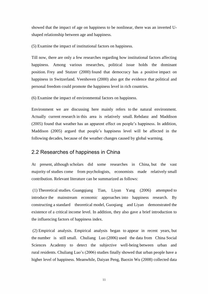
Based on these assumptions, we can use the utility theory of microeconomics to

explain the relationship between wealth and happiness (see Figure 3.1).

Utility depends on the absolute number of consumer goods. And maximizing utility is

limited by income budget, so an increase in income could expand consumers‟

choice set and eventually improve the utility level.

Figure 3.1 Variation tendency of Utility when income increases

15

And utility refers to the total satisfaction people obtained from consumptions. Thus,

we can also say that an increase in income could enhance people‟s total satisfaction

(happiness).

However, people are not constantly pursuit of behavior maximization. When making

a decision, many issues should be considered. Particularly, in some cases, people are

irrational; some psychological factors will greatly influence people‟s behavior.

In 1974, Easterlin‟s finding firstly questioned the conclusion (the growth of income

could enhance people‟s happiness). Using the data from happiness survey, Easterlin

found that although U.S. experienced a booming in per capita income, the

observed level of happiness did not have a corresponding increase. This finding was

later known as the "Easterlin paradox", or "income paradox". At the same time, data

from other developed countries also showed the same results. From this, it can be seen

that relationship between wealth and happiness is more complicated than we thought.

Does "Easterlin paradox" imply economic development is pointless? We strongly

believe that the answer to this question is no. Gary S. Becker (2007), Nobel

economics prize winner in 1992, noted that individual is mainly concerned not with

his absolute level of success, but rather with the difference between his success and a

benchmark that changes over time. Frankly speaking, utility is mainly depended on

the relative level of an individual‟s economic conditions. Therefore, although local

economy developed very fast, people do not have a corresponding growth of

happiness.

Besides, Becker (2010) argued that when seeking utility maximization, people should

consider many types of non-economic factors, such as human behavior, time, etc. In

Gary‟s point of view, the following inputs are essential for producing happiness:

market goods, time, and human capital. For instance, some people in Sweden are very

into skiing, they may need: (1) ski suit, ski goggles, and a ride to snow mountain, (2)

a free morning and (3) the ability to ski as well as the knowledge that skiing leads to

happiness in their particular brain. Note that simply buying high-quality skiing

instruments will have very little effect here, because both time and human capital are

essential components. And economic development could directly or indirectly

16

increases the availability of all these three inputs. To some extent, we can say that

economic development has a positive effect on happiness.

In addition, Becker gave a simple explanation regarding why happiness surveys failed

to show a robust and strong relationship between income growth and happiness.

Becker (2010) argues that this link is weak because we are only beginning to learn

how happiness can and cannot be produced. As happiness science matures and its

findings are communicated to the general public, it is reasonable to expect a stronger

link to emerge.

17

4. Data and model description

4.1 Data sources

At present, data used by international scholars mainly come from psychologists

and sociologists‟ surveys. Among them, the most famous one is World Value Survey

(WVS) presided by Professor Ronald Inglehart in Michigan University. The others

include General Social Survey (GSS) sponsored by University of Chicago, Euro

barometer Surveys, German Socio-Economic Panel, etc. A great number of data are

collected continuously for decades, but some of them are also panel data. In contrast,

the investigation for Chinese happiness index is very rare. Currently there are only

two sources of data:

One source is WVS, we have already mentioned earlier. WVS is a worldwide project

in dozens of countries or regions. But countries or regions involved into the

investigations are not exactly the same each year. Since 1981, WVS has conducted 5

waves of investigation. From the second time, China started to participate in this

project, so we can get four collections of data from WVS.

Another source is China General Social Survey (CGSS) co-chaired by Renmin

University of China and Hong Kong University of Science &

Technology. CGSS began to investigate since 2003. So far, 4 investigation results are

available to the public. CGSS adopted the way of random sampling and Door to Door

Interview, the data quality is considered to be very reliable.

This paper uses the data of CGSS in 2006. The data belongs to the micro-level cross-

sectional data. Reasons of using CGSS data in 2006 can be divided into 4 aspects:

(1) The latest data of WVS is published in 2005, to some extent, data of CGSS in

2006 is relatively new. (2) Compared to WVS data, CGSS has a larger sample

size. CGSS includes 10372 samples in 2006; but the largest sample for WVS

is only 2015. (3) Credibility of CGSS survey is very high. Statistically, interviewees‟

cooperation rate has reached 98%, which shows a high reliability of survey results.

(4) WVS is a worldwide survey, the design of questionnaire cannot

adequately reflect the specific situation of China. However, questionnaire of CGSS

18

fully considers the particular conditions in China. In view of the above reasons, the

section of empirical analysis uses the data of CGSS in 2006.

4.2 Variable Description

4.2.1 Definition and its Descriptive statistics

On the basis of the literature review, we introduce the following variables into the

basic regression model:

Income: personal absolute income in 2005 (unit: 1 RMB)

Gender: dummy variable, male=1, female=0

Age: interviewees‟ age in 2005

Health: health status can be divided into 6 categories; extremely good=1,

extremely bad=6

Marital status

Married: dummy variable means interviewees who are married, reference group

is single; married=1, other=0

Divorced: dummy variable, reference group is single; divorced=1, other=0

Widowed: dummy variable, which means interviewees‟ spouse has dead,

reference group is single; widowed=1, other=0

Employment

Employed: dummy variable, reference group is unemployed; employed=1,

other=0

Retired: dummy variable, reference group is unemployed; retired=1, other=0

Learning: dummy variable, which means people are still in school,

reference group is unemployed; learning=1, other=0

Education: dummy variable, interviewee who got a college degree or above=1,

other=0

Urban/suburb: according to the Book of Registered Permanent Residence, we

can distinguish people who live in urban or suburb area; urban=1, suburb=0

19

Communication: this variable measures the closeness of interviewees with

friends and relatives. Communication can be divided into 5 categories; very not

close with friends and relatives=1, very close with friends and relatives=5

Happy: interviewees‟ sense of happiness can be divided into 5 categories; very

unhappy=1, very happy=5

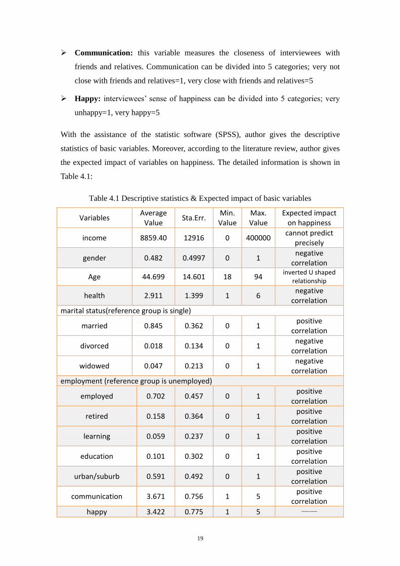
With the assistance of the statistic software (SPSS), author gives the descriptive

statistics of basic variables. Moreover, according to the literature review, author gives

the expected impact of variables on happiness. The detailed information is shown in

Table 4.1:

Table 4.1 Descriptive statistics & Expected impact of basic variables

Variables Average

Value Sta.Err.

Min. Value

Max. Value

Expected impact on happiness

income 8859.40 12916 0 400000 cannot predict

precisely

gender 0.482 0.4997 0 1 negative

correlation

Age 44.699 14.601 18 94 inverted U shaped

relationship

health 2.911 1.399 1 6 negative

correlation

marital status(reference group is single)

married 0.845 0.362 0 1 positive

correlation

divorced 0.018 0.134 0 1 negative

correlation

widowed 0.047 0.213 0 1 negative

correlation

employment (reference group is unemployed)

employed 0.702 0.457 0 1 positive

correlation

retired 0.158 0.364 0 1 positive

correlation

learning 0.059 0.237 0 1 positive

correlation

education 0.101 0.302 0 1 positive

correlation

urban/suburb 0.591 0.492 0 1 positive

correlation

communication 3.671 0.756 1 5 positive

correlation

happy 3.422 0.775 1 5 ——

20

4.2.2 Test for multicollinearity

In a regression model, two or more independent variables are highly correlated will

cause the problem of multicollinearity. Hill et al (2008) argued that if correlation

between any pairs of variables exceeds 0.7, then one of the variables should be

excluded from regression. Multicollinearity problem can affect the

accuracy of the regression results in many aspects. Thus, before running the

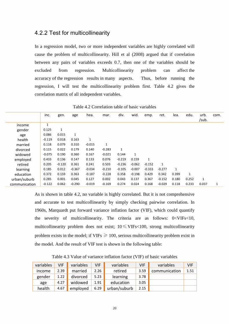
regression, I will test the multicollinearity problem first. Table 4.2 gives the

correlation matrix of all independent variables.

Table 4.2 Correlation table of basic variables

As is shown in table 4.2, no variable is highly correlated. But it is not comprehensive

and accurate to test multicollinearity by simply checking pairwise correlation. In

1960s, Marquardt put forward variance inflation factor (VIF), which could quantify

the severity of multicollinearity. The criteria are as follows: 0<VIFs<10,

multicollinearity problem does not exist; 10≤VIFs<100, strong multicollinearity

problem exists in the model; if VIFs ≥ 100, serious multicollinearity problem exist in

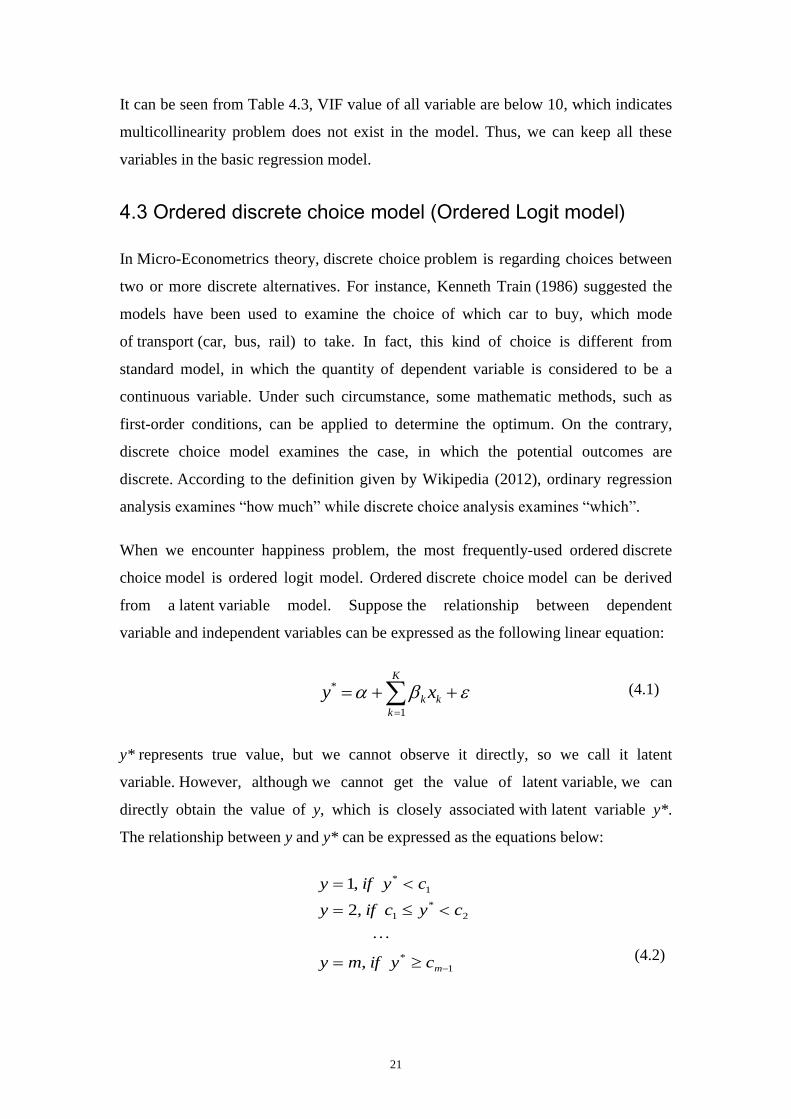
the model. And the result of VIF test is shown in the following table:

Table 4.3 Value of variance inflation factor (VIF) of basic variables

variables VIF variables VIF variables VIF variables VIF

income 2.39 married 2.26 retired 3.59 communication 1.51

gender 1.22 divorced 5.23 learning 3.78

age 4.27 widowed 1.91 education 3.05

health 4.67 employed 6.29 urban/suburb 2.15

inc. gen. age hea. mar. div. wid. emp. ret. lea. edu. urb. /sub.

com.

income 1

gender 0.125 1

age 0.086 0.015 1

health -0.119 0.018 0.163 1

married 0.118 0.079 0.310 -0.015 1

divorced 0.115 0.022 0.179 0.140 -0.283 1

widowed -0.075 0.190 0.360 0.167 -0.021 0.144 1

employed 0.433 0.136 0.147 0.133 0.076 -0.219 0.159 1

retired 0.205 -0.120 0.361 0.241 0.503 -0.236 -0.062 -0.152 1

learning 0.185 0.012 -0.367 -0.034 -0.210 -0.105 -0.007 -0.333 -0.277 1

education 0.372 0.159 0.363 -0.187 -0.228 0.358 -0.198 0.429 0.342 0.399 1

urban/suburb 0.285 0.001 0.045 0.127 0.002 0.043 0.137 0.367 -0.152 0.180 0.252 1

communication -0.122 0.062 -0.290 -0.019 -0.169 0.274 0.024 0.168 -0.029 0.118 0.233 0.037 1

21

It can be seen from Table 4.3, VIF value of all variable are below 10, which indicates

multicollinearity problem does not exist in the model. Thus, we can keep all these

variables in the basic regression model.

4.3 Ordered discrete choice model (Ordered Logit model)

In Micro-Econometrics theory, discrete choice problem is regarding choices between

two or more discrete alternatives. For instance, Kenneth Train (1986) suggested the

models have been used to examine the choice of which car to buy, which mode

of transport (car, bus, rail) to take. In fact, this kind of choice is different from

standard model, in which the quantity of dependent variable is considered to be a

continuous variable. Under such circumstance, some mathematic methods, such as

first-order conditions, can be applied to determine the optimum. On the contrary,

discrete choice model examines the case, in which the potential outcomes are

discrete. According to the definition given by Wikipedia (2012), ordinary regression

analysis examines “how much” while discrete choice analysis examines “which”.

When we encounter happiness problem, the most frequently-used ordered discrete

choice model is ordered logit model. Ordered discrete choice model can be derived

from a latent variable model. Suppose the relationship between dependent

variable and independent variables can be expressed as the following linear equation:

K

k

kk xy1

*

y* represents true value, but we cannot observe it directly, so we call it latent

variable. However, although we cannot get the value of latent variable, we can

directly obtain the value of y, which is closely associated with latent variable y*.

The relationship between y and y* can be expressed as the equations below:

1

*

2

*

1

1

*

,

,2

,1

mcyifmy

cycify

cyify

(4.1)

(4.2)

22

Thereinto, 121 ,,c mcc are called cut point. Obviously if there are m categories of

variables, it will be m-1 cut points.

Therefore, for a given value of x, the cumulative probability equation can be

expressed as follows:

K

k

kkj

K

k

kkjj

K

k

kkj

xF

xcPcxPcyPxjP

1

11

*

c

y

For the Ordered Logit Model, we assume that the error term subject to the

logistic distribution, the definition is listed as follows:

ye

xFx

1

1

The inverse function is:

y

yyFx

1ln1

Therefore, we can derived from equation (4.3)

xjyP

xjyPxjPFxc

K

k

kkj1

lny1

1

Generally, we call the right side of equation (4.6) is the logit form of y, or yogitL .

And usually we put yogitL at the left side, so the equation can be written as:

K

k

kkj xcxjyP

xjyP

11ln

It can be seen that there is a linear relationship between independent variable x and

yogitL , but the linear relationship does not exist between x and y

itself. Through regression, we can estimate the value of each coefficient, thus we can

see the influencing extent of each independent variables on yogitL . xjyP is the

(4.6)

(4.7)

(4.3)

(4.4)

(4.5)

23

probability of occurrence of certain circumstances, xjyP 1 is the probability of

an event that is not going to happen, the ratio is called “odds”. In this way, yogitL

can be treated as the log of occurrence ratio. Thus, although we cannot directly see the

relationship between x and y, we can detect the impact of x on log of odds.

4.4 Specific format of discrete choice model in this paper

The discrete choice model mentioned above is a generalized model. In order

to analyze the particular situation in this paper, we need to modify this model

more specific.

The true level of happiness depends on a number of variables, and there is

a linear relationship between the true level of happiness and independent variables,

namely:

K

k

kk xHAPPY1

*

However, we are not able to observe people's real level of happiness ( *HAPPY ), we

can only get the value of happiness ( HAPPY ) when people answered during the

interview. The relationship between people‟s true level of happiness and their answers

can be described as follows:

4

*

4

*

3

3

*

2

2

*

1

1

*

if)"happyVery("5

if)"Happy("4

if)"Average("3

if)"Unhappy("2

if)"unhappyVery("1

cHAPPYHAPPY

cHAPPYcHAPPY

cHAPPYcHAPPY

cHAPPYcHAPPY

cHAPPYHAPPY

，

，

，

，

，

Since we are able to get the answers of people‟s happiness level, we can estimate the

coefficients of each independent variable through regression. Ordered logit regression

equation is:

K

k

kkj xcxjHAPPYP

xjHAPPYP

11ln

(4.8)

(4.9)

(4.10)

24

This formula expresses the ratio people tend to answer a lower level of happiness to a

higher level. That is, if the value of the left side increases, people are

more inclined to answer a lower level of happiness.

Therefore, according to the coefficients of variables at the right side, we can see a

change of a variable will lead people to answer a higher level of happiness or a lower

level. For instance, if the sign of coefficient of variable income is positive, it indicates

that the growth of income will make log odds reduce, i.e. the probability of answering

a lower level of happiness will decrease. Or we can say that an increase in

income can enhance people's happiness level.

25

5. Empirical analysis

5.1 Basic regression results

Statistic software SPSS has the function of ordered logit regression, so this paper

used SPSS to carry on empirical analysis, Table 5.1 gives the basic regression results:

Table 5.1 Basic regression result

income/1000 0.016***

(7.28)

gender -0.112**

(-2.27)

age -0.092***

(-8.98)

age2

0.001*** (9.12)

health -0.363*** (-20.74)

marital status (reference group is single)

married 0.921***

(9.23)

divorced -0.348* (-1.73)

widowed -0.023 (-0.14)

employment (reference group is unemployed)

employed 0.335***

(3.25)

retired 0.534***

(4.86)

learning 0.521***

(3.99)

education 0.419***

(4.53)

urban/suburb 0.078 (1.02)

communication 0.587*** (18.35)

Pseudo R2 0.078

Number of samples 9328

Note: t-statistics based on robust standard errors in parentheses. *, ** and ***

denote significance at the 10, 5 and 1 percentage level, respectively.

Gender. Regression result shows that coefficient of dummy

variable gender is significant, the sign of gender is negative, which indicates that

male‟s happiness level is lower than female. This result is broadly consistent with

existing research results in China. To some extent, it may reflect male‟s pressure

26

is generally bigger than female in Chinese society.

Age As shown in the literature review, we can expect that the impact of age on

happiness to be nonlinear, so both age and age2 are introduced in the regression

model. Actually, regression result confirms this point of view. The signs of

coefficient of age and age2 are negative and positive, respectively. And both

coefficients of these 2 variables are significant. This result indicates that there is a

"U" shaped relationship between age and happiness. After student life,

people's happiness level tends to decrease with the growth of age over time.

However, after a certain point, people‟s happiness level will continuously growth.

According to the data provided by CGSS, we can roughly calculate that the least

happy age is 47. This result is roughly consistent with our previous

experience: before the age of 50, people always take big burdens, spend a lot of

energy and time in earning money to live a better life.

Health. It has been mentioned in literature review, health has a positive influence

on happiness. Regression result also confirms this point of view. The sign of

coefficient of health is negative, which indicates that improvement in health

can increase the level of happiness.

Marital status. In the regression equation, marital status is represented by three

dummy variables: married, divorced and widowed, the reference group is single.

The coefficient of variable married is significant and the sign is positive, which

indicates that married people has a higher level of happiness. Coefficient of

divorced is significant at 10 percentage level, and the sign is negative. Although

coefficient of widowed is not significant, the sign is negative. All these results are

relatively in line with people's intuition.

Employment. As we discussed in literature review, employment is a key factor

affecting residents' happiness. In fact, regression result confirms

these conclusions. In this section, employment situation is also represented by

three dummy variables: employed, retired and learning, the reference group is

unemployed. The sign of coefficients of three dummy variables are positive, and

coefficients of them are significant. This result suggests that compared to

unemployed people, other people have a better feeling of happiness.

27

Educational. In this section, education is also defined as a dummy variable,

which is used to distinguish people whether has a college degree or above.

The coefficient of education is significant and the sign is positive, which

means highly educated residents have a higher level of happiness.

Living place. In this section, a dummy variable is used to separate people live in

urban or rural area. The sign is positive, but the coefficient is insignificant.

Result shows that living place does not have an apparent effect on residents‟

happiness.

Social interaction. This part uses the relationship with relatives and friends

to reflect people‟s social interaction. Regression result shows coefficient of this

variable is significant and the sign of communication is positive, which suggests

that if people communicate with others frequently, they will obtain

a higher level of happiness.

The conclusions we discussed above are only basic results from the model. We

will consider different forms of equations in the following sections, so as to get more

detailed results.

5.2 Introduce income2 into the model

The revival of interest in analyzing happiness problem is mainly due to the so-called

Paradox of Happiness. This paradox stems from Easterlin‟s study: since World War II,

although per capita income increased significantly, the observed level

of happiness did not appear a corresponding growth.

Does China also exist this phenomenon? The following tendency chart can more or

less give us an answer. Because the design of questionnaires is not exactly the same in

CGSS among different years, this paper drew the chart, on the basis of the data from

WVS.

28

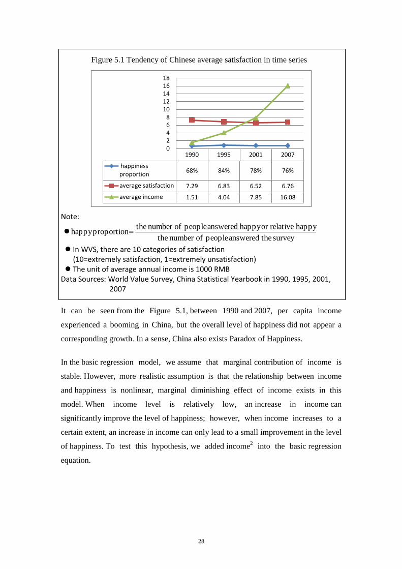
Note:

surveytheansweredpeopleofnumberthe

happyrelativeorhappyansweredpeopleofnumbertheproportionhappy

In WVS, there are 10 categories of satisfaction (10=extremely satisfaction, 1=extremely unsatisfaction)

The unit of average annual income is 1000 RMB Data Sources: World Value Survey, China Statistical Yearbook in 1990, 1995, 2001,

2007

It can be seen from the Figure 5.1, between 1990 and 2007, per capita income

experienced a booming in China, but the overall level of happiness did not appear a

corresponding growth. In a sense, China also exists Paradox of Happiness.

In the basic regression model, we assume that marginal contribution of income is

stable. However, more realistic assumption is that the relationship between income

and happiness is nonlinear, marginal diminishing effect of income exists in this

model. When income level is relatively low, an increase in income can

significantly improve the level of happiness; however, when income increases to a

certain extent, an increase in income can only lead to a small improvement in the level

of happiness. To test this hypothesis, we added income2 into the basic regression

equation.

1990 1995 2001 2007

happiness proportion

68% 84% 78% 76%

average satisfaction 7.29 6.83 6.52 6.76

average income 1.51 4.04 7.85 16.08

02468

1012141618

Figure 5.1 Tendency of Chinese average satisfaction in time series

29

Table 5.2 Result of adding income2 into the regression model

income/1000 0.019***

(7.34)

income2

-1.90e-5

*** (-5.93)

gender -0.069* (-1.78)

age -0.091***

(-8.35)

age2

0.001*** (7.97)

health -0.366*** (-20.49)

marital status (reference group is single)

married 0.974***

(9.46)

divorced -0.306 (-1.08)

widowed 0.031 (0.19)

employment (reference group is unemployed)

employed 0.378***

(3.93)

retired 0.552***

(4.70)

learning 0.489***

(4.11)

education 0.465***

(5.90)

urban/suburb 0.100 (1.55)

communication 0.586*** (19.52)

Pseudo R2 0.079

Number of samples 9328

Note: t-statistics based on robust standard errors in parentheses. *, ** and ***

denote significance at the 10, 5 and 1 percentage level, respectively.

From the regression result in Table 5.2, we can find that there is no significant change

of coefficient of other variables when adding income2 into the model. The

signs of coefficient of income and income2 are positive and negative, respectively.

This result is expected to be consistent with our previous studies mentioned in

literature review. This finding also suggests that there is a reversed U relationship

between income and happiness.

Actually Chinese government has formulated an income standard (poverty line)

in 2003, namely if residents‟ income is less than 1300 yuan, they will be considered

as the low-income people. Based on the empirical result, we can get the conclusion

30

that if someone‟s income is below poverty line, the growth of income is expected to

have a great impact on happiness; if resident‟s income is above poverty line,

income has relatively small effect on happiness. In order to verify this hypothesis, this

paper calculated the marginal effect of income on happiness.2 Thus, we can

effectively see the response of income changes from two different groups (residents‟

personal income <1300 & residents‟ personal income≥1300).

Table 5.3 Marginal effect of income on happiness

personal income <1300 yuan personal income≥1300

yuan

x

HAPPYP

)1(

-0.332 -2.67 e-4

x

HAPPYP

)2(

0.097 -1.29 e-3

x

HAPPYP

)3(

0.197 -1.50 e-3

x

HAPPYP

)4(

0.037 2.53 e-3

x

HAPPYP

)5(

1.07e-3 5.43 e-4

Looking at Table 5.3 we see that for the group of residents, whose income

is less than 1300 yuan, If income increases 1000 yuan, the probability of answering

"very unhappy” (HAPPY = 1) will decrease approximately 33.2%, the probability of

answering "very happy" (HAPPY = 5) will go up 0.1%. For the group of residents,

whose income is more than 1300 yuan, If income increases 1000 yuan, the

probability of answering "very unhappy” (HAPPY = 1) will decrease 0.027%, the

probability of answering "very happy" (HAPPY = 5) will raise 0.054%. Thus, it can

be seen that the fluctuation of income has greater impact on low-income people than

the middle and high income earners.

5.3 Introduce relative income into the model

When evaluating happiness level, people always compare their own situation with

subjective standard. This standard is determined by themselves and the average level

of society. Simply put, people like to use a series of references to assess their own

happiness. Therefore, the impact path of relative income mainly comes from various

types of social comparison theory (Alpizar et al, 2005).

2. Derivation of marginal effect function can be found in Appendix 1.

We can also get the value of marginal contribution via statistic software SPSS.

31

On the one hand, people like to compare their income with others. Thus, it is relative

income that determines one‟s happiness, instead of absolute income. In this way, if a

person's relative income increases (absolute income increases, other people‟s wealth

does not appear a corresponding growth), his/her happiness level will experience a

growth. Therefore, it makes easy to explain why the overall level of happiness does

not significantly improve after a booming in one region‟s economy. Another

manifestation of relative income is Adaptation Level Theory, which emphasizes the

adaptability of people. People have their own expectation, and they like to

compare their income with their own expectation. If income reaches or exceeds their

expectation, people tend to feel happier.

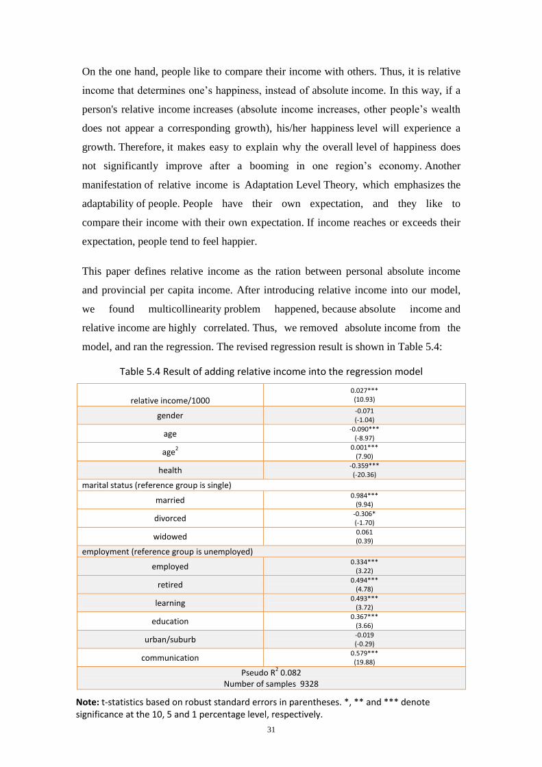
This paper defines relative income as the ration between personal absolute income

and provincial per capita income. After introducing relative income into our model,

we found multicollinearity problem happened, because absolute income and

relative income are highly correlated. Thus, we removed absolute income from the

model, and ran the regression. The revised regression result is shown in Table 5.4:

Table 5.4 Result of adding relative income into the regression model

relative income/1000 0.027*** (10.93)

gender -0.071 (-1.04)

age -0.090***

(-8.97)

age2

0.001*** (7.90)

health -0.359*** (-20.36)

marital status (reference group is single)

married 0.984***

(9.94)

divorced -0.306* (-1.70)

widowed 0.061 (0.39)

employment (reference group is unemployed)

employed 0.334***

(3.22)

retired 0.494***

(4.78)

learning 0.493***

(3.72)

education 0.367***

(3.66)

urban/suburb -0.019 (-0.29)

communication 0.579*** (19.88)

Pseudo R2 0.082

Number of samples 9328

Note: t-statistics based on robust standard errors in parentheses. *, ** and *** denote significance at the 10, 5 and 1 percentage level, respectively.

32

Coefficient of relative income is 0.027, and this variable is significant at 1% statistical

level. And R2 increases from 0.079 to 0.082. Regression result suggests that relative

income has a closer relationship with residents' happiness. This conclusion

is consistent with our hypothesis.

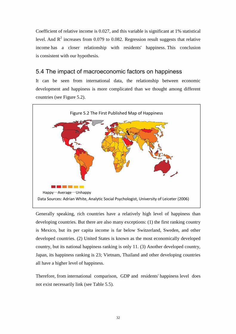
5.4 The impact of macroeconomic factors on happiness

It can be seen from international data, the relationship between economic

development and happiness is more complicated than we thought among different

countries (see Figure 5.2).

Generally speaking, rich countries have a relatively high level of happiness than

developing countries. But there are also many exceptions: (1) the first ranking country

is Mexico, but its per capita income is far below Switzerland, Sweden, and other

developed countries. (2) United States is known as the most economically developed

country, but its national happiness ranking is only 11. (3) Another developed country,

Japan, its happiness ranking is 23; Vietnam, Thailand and other developing countries

all have a higher level of happiness.

Therefore, from international comparison, GDP and residents' happiness level does

not exist necessarily link (see Table 5.5).

Figure 5.2 The First Published Map of Happiness

Happy—Average—Unhappy

Data Sources: Adrian White, Analytic Social Psychologist, University of Leiceter (2006)

33

Table 5.5 National Happiness Level Ranking.

Ranking Country Number of

samples

Average value of

residents‟ happiness

Standard

deviation

1 Mexico 1512 8.23 2.053

2 Switzerland 1232 7.91 1.625

3 Finland 1014 7.84 1.747

4 Sweden 1002 7.72 1.608

5 Argentina 995 7.7 1.919

6 Brazil 1495 7.64 2.113

7 Turkey 1346 7.46 2.237

8 Cyprus 1050 7.35 2.029

9 Spain 1195 7.31 1.502

10 Australia 1410 7.3 1.797

11 United States 1241 7.26 1.767

12 Trinidad and Tobago 999 7.26 2.225

13 Brunei 980 7.24 1.777

14 Chile 992 7.24 2.036

15 Slovenia 1033 7.24 1.951

16 Thailand 1532 7.21 1.806

17 South Africa 2977 7.2 2.378

18 Jordan 1197 7.2 2.797

19 Andorra 1003 7.14 1.619

20 Vietnam 1482 7.09 1.891

21 Poland 989 7.02 2.075

22 Peru 1490 7.02 2.229

23 Japan 1080 6.99 1.809

24 Indonesia 1906 6.91 2.157

25 Italy 1006 6.89 1.742

26 Malaysia 1200 6.84 1.789

27 China 1959 6.76 2.4

28 Taiwan 1227 6.66 2.07

29 Germany 1070 6.62 2.128

30 Korea 1197 6.39 1.959

31 Ghana 1528 6.12 2.629

32 Mali 1430 6.09 2.592

33 Zambia 1463 6.06 2.497

34 serbia 1175 6.01 2.087

35 Ukraine 996 5.81 2.307

36 India 1954 5.79 2.351

37 Egypt 3050 5.78 2.684

38 Roumania 1658 5.75 2.385

39 burkina faso 1499 5.57 2.181

40 Moldova 1041 5.45 2.261

Data Sources: World Value Survey, 2007

Similarly, we should also consider other macroeconomic factors, such as economic

growth rate, income distribution into our analysis.

34

5.4.1 GDP per capita on happiness

The following discussion will take every province as a unit, to examine the impact of

provincial economic level on happiness. This paper uses GDP per capita of every

province to represent the development level of local economy. Following table shows

the regression result.

Table 5.6 Result of adding GDP per capita into the regression model

income/1000 0.016***

(6.16)

income2

-1.52e-05*** (-4.21)

gender -0.083** (-2.09)

age -0.090***

(-7.94)

age2

0.001*** (8.75)

health -0.352*** (-19.84)

marital status (reference group is single)

married 0.998***

(9.43)

divorced -0.294* (-1.82)

widowed 0.116 (0.77)

employment (reference group is unemployed)

employed 0.270***

(3.10)

retired 0.326***

(2.62)

learning 0.507***

(4.16)

education 0.295***

(3.82)

Urban/suburb 0.184 (1.06)

communication 0.566*** (17.29)

GDP per capita 0.001 (0.02)

Pseudo R2 0.092

Number of samples 9328

Note: t-statistics based on robust standard errors in parentheses. *, ** and ***

denote significance at the 10, 5 and 1 percentage level, respectively.

From Table 5.6, we can see that GDP per capita does not show a great impact on

residents‟ happiness. This result indicates that from a macro point of view, there is no

significant relationship between overall economic level of one regional and its

residents' happiness.

35

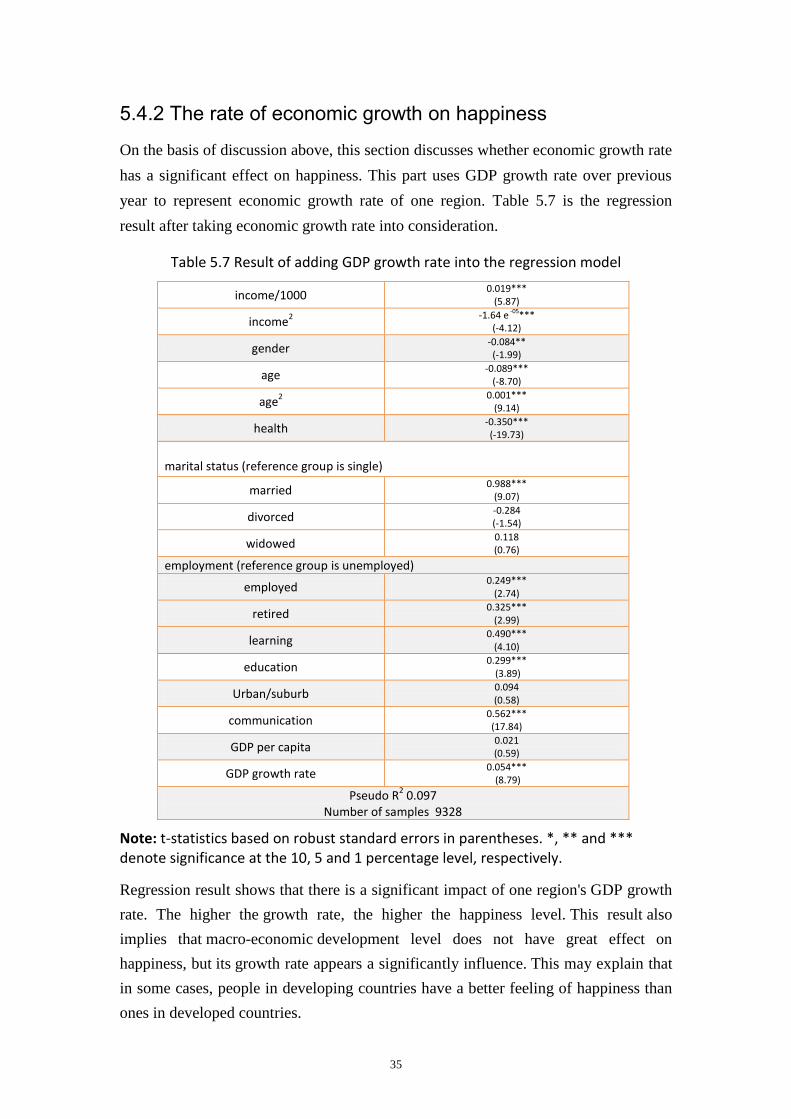
5.4.2 The rate of economic growth on happiness

On the basis of discussion above, this section discusses whether economic growth rate

has a significant effect on happiness. This part uses GDP growth rate over previous

year to represent economic growth rate of one region. Table 5.7 is the regression

result after taking economic growth rate into consideration.

Table 5.7 Result of adding GDP growth rate into the regression model

income/1000 0.019***

(5.87)

income2

-1.64 e -05*** (-4.12)

gender -0.084** (-1.99)

age -0.089***

(-8.70)

age2

0.001*** (9.14)

health -0.350*** (-19.73)

marital status (reference group is single)

married 0.988***

(9.07)

divorced -0.284 (-1.54)

widowed 0.118 (0.76)

employment (reference group is unemployed)

employed 0.249***

(2.74)

retired 0.325***

(2.99)

learning 0.490***

(4.10)

education 0.299***

(3.89)

Urban/suburb 0.094 (0.58)

communication 0.562*** (17.84)

GDP per capita 0.021 (0.59)

GDP growth rate 0.054***

(8.79)

Pseudo R2 0.097

Number of samples 9328

Note: t-statistics based on robust standard errors in parentheses. *, ** and *** denote significance at the 10, 5 and 1 percentage level, respectively.

Regression result shows that there is a significant impact of one region's GDP growth

rate. The higher the growth rate, the higher the happiness level. This result also

implies that macro-economic development level does not have great effect on

happiness, but its growth rate appears a significantly influence. This may explain that

in some cases, people in developing countries have a better feeling of happiness than

ones in developed countries.

36

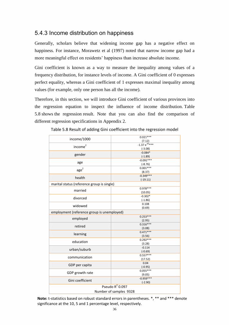
5.4.3 Income distribution on happiness

Generally, scholars believe that widening income gap has a negative effect on

happiness. For instance, Morawetz et al (1997) noted that narrow income gap had a

more meaningful effect on residents‟ happiness than increase absolute income.

Gini coefficient is known as a way to measure the inequality among values of a

frequency distribution, for instance levels of income. A Gini coefficient of 0 expresses

perfect equality, whereas a Gini coefficient of 1 expresses maximal inequality among

values (for example, only one person has all the income).

Therefore, in this section, we will introduce Gini coefficient of various provinces into

the regression equation to inspect the influence of income distribution. Table

5.8 shows the regression result. Note that you can also find the comparison of

different regression specifications in Appendix 2.

Table 5.8 Result of adding Gini coefficient into the regression model

income/1000 0.021***

(7.12)

income2

-1.37 e-05*** (-3.08)

gender -0.084* (-1.89)

age -0.091***

(-8.76)

age2

0.001*** (8.37)

health -0.349*** (-19.11)

marital status (reference group is single)

married 0.978*** (10.05)

divorced -0.302* (-1.86)

widowed 0.108 (0.69)

employment (reference group is unemployed)

employed 0.253***

(2.95)

retired 0.316***

(3.08)

learning 0.471***

(3.56)

education 0.292***

(3.28)

urban/suburb -0.114 (-0.69)

communication 0.557*** (17.52)

GDP per capita 0.04

(-0.95)

GDP growth rate 0.055***

(9.05)

Gini coefficient -0.959***

(-2.90)

Pseudo R2 0.097

Number of samples 9328

Note: t-statistics based on robust standard errors in parentheses. *, ** and *** denote significance at the 10, 5 and 1 percentage level, respectively.

37

Regression result shows that coefficient of Gini coefficient is significant at 1%

statistical level and the sign of Gini coefficient is negative, which indicates that the

higher the Gini coefficient, the lower the happiness level. Or we can say that the

inequality of income distribution increases will lead to a reduction of

residents' happiness. This conclusion is consistent with our forecast.

38

6. Policy recommendation

Different layers of the society have different demands, thus every individual‟s

feeling of happiness is not exactly the same. Because of the divergence in

preferences, people with various incomes will make different contributions to the

happiness index. In this way, when carrying out a new policy, government may take

all kinds of people‟s needs into consideration, try to ensure the maximum utility of

residents. Considering the actual situation in China, the vast majority of population

are middle and lower income workers, farmers, and unemployed; their living standard

determines the overall level of happiness in society. Therefore, it is very urgent and of

great importance to design proper policies to enhance these people‟s happiness level.

(1) Guide sustainable and stable development of economics

Maslow's Hierarchy of Needs Theory argues that survive is the basic need of human

beings, it is the foundation of other demands. Security, marriage, communication,

self-fulfillment, etc can never be achieved without the support of certain material base.

Only when income satisfies people‟s basic needs; safety, health, attitude, environment

and other non-material factors can show a greater impact on happiness. Therefore,

although income is not a sufficient condition of happiness, it is a necessary condition

of happiness. In fact, empirical analysis we talked above confirmed the vital role of

income on individual‟s happiness.

Before income increased to a certain level, income has a great impact on happiness.

Compared to western countries, Chinese residents' income is generally low, there is

still a big gap in material living conditions between China and developed countries.

Consequently, during a certain period, it is of great significance to raise residents‟

income. In fact, a good state of economy is very critical to both individuals and

society. It is quite essential to vigorously develop economy, in order to meet the

increasing material and culture needs of residents.

(2) Regulate wealth gap between rich and poor

Previous studies have shown that income distribution is an extremely important

factor to affect overall level of happiness. Social Comparison Theory also argues that

income distribution is the core factor in determining happiness index. In addition,

39

empirical analysis found that unfair distribution of income will lead to a lower level of

happiness. We may take some measures to regular income gap between individuals,

control the excessive imbalance of income distribution.

As shown in the literature review, we can expect that there is an inverted U-shaped

relationship between wealth gap and economic growth. The expansion of wealth gap

between rich and poor is an inevitable problem in the process of economic

development, which requires the regulation carried out by the government. To this

end, government can proceed from the following aspects: firstly, improve tax and

transfer payment system, so as to complete the redistribution of social wealth. Second,

speed up the process of social transformation in legal system, accelerate the pace of

marketization in monopoly industries, and create a just, fair and open environment for

income distribution. Finally, take more efforts to develop backward areas, for instance,

guide capital, technology and human resources to the less developed areas, and

ultimately improve the income level, narrow the wealth gap between rich and poor.

(3) Build a sound social security system, try to reduce unemployment

Currently it remains a primary priority on Chinese government's working agenda to

make Chinese residents live better lives and satisfy their needs for material and

cultural fulfillments. To improve the overall level of happiness, government should

build a sound social security system to protect the middle and lower income residents

In addition, Di Tella, MacCulloch, and Oswald (2003) argued that the unemployed

have the lowest feeling of happiness in society. The unemployed are lack of income

sources; particularly, their sense of self-realization is seriously hampered.

In order to reduce the unemployment rate and increase unemployed people‟s

happiness, on one hand, government has to adjust economic structure, improve the

demand and absorptive capacity for labor; on the other hand, administrative unit need

to spread unemployment insurance, which could improve the basic living

standard of unemployed or laid-off workers.

40

7. Conclusions and further study directions

7.1 Some conclusions

Based on the original researches, this paper mainly carried on an empirical study in

Chinese happiness index via ordered discrete choice model. Author tried to overcome

the deficiencies of the previous studies, for example, the selected sample size is much

larger than before, data credibility is relatively high. Variables, such as age, gender,

marital status, employment, passed the significance test, which suggests that these

factors have great influence on happiness index. In support of the basic regression

result, this paper undertook a systematic analysis on income, and finally concluded

that “paradox of happiness” also exists in China. Besides, there are only a few

literatures mentioning macroeconomic variables. This article introduced GDP,

economic growth rate, income distribution into our discussion. Ultimately we drew

the conclusion that GDP did not has a great influence on residents‟ happiness, but

both economic growth rate and income distribution had a significant impact on

happiness. And one innovative point is that from the perspective of government,

author put forward a number of policy recommendations; for example, establish

transfer payment system, adjust economic structure, etc.

7.2 further study suggestions

Further research suggestions can be summarized as the following aspects:

(1) the most severe constrain of relevant researches is data, so it is very essential to

establish a high-quality database. Western countries used large-scale panel data to

carry on researches, but in China, there is no national time-series data available to the

public. However, this task cannot be completed by a person or an institution in a short

time. Therefore we need more scholars, who can put efforts and patience in this area.

(2) We should adopt more advanced tools and methods to undertake analysis. On the

basis of the latest studies, the method of panel data will occupy the leading position in

the future. However, Easterlin used the demographic method to do the time series

analysis, which also plays an instructive role in this field of study.

41

(3) We should learn lessons from other disciplines. Current researches of

Chinese happiness index still use some mainstream ways to analyze. We should

introduce psychology, demographic, biology and other approaches into our research.

In addition, experimental study may have important reference for the study of

happiness. For instance, when we encounter some findings that we are unsure, we can

introduce an experiment to test the hypothesis.

(4) Because of the constraint of information, this paper ignored some variables when

doing empirical research. Further studies could consider the impact of personality

factors, institutional factors and environmental factors on happiness. At the same

time, due to the lack of time series data, this paper can not introduce lagged variables

into the regression model. Hopefully, future scholars could do some works to

compensate the deficiencies in this field.

(5) Many countries have a higher level of happiness, such as some Nordic countries.

We can compare Chinese economical data or social security system with those

countries. Through comparison, we can detect some deeper reasons to guide our new

research.

42

References:

[1] Alpizar, Francisco; Carlsson, Fredrik; Johansson-Stenman, Olof. How much do we

care about absolute versus relative income and consumption? Journal of Economic

Behavior & Organization 2005, 56: 405–421

[2] Becker, Gary S. Habits, Peers, and Happiness: An Evolutionary Perspective. The

American Economic Review, 2007, 97: 487-491

[3] Becker, Gary S. Happiness, Income and Economic Policy. Institute for Economic

Research at the University of Munich, 2010, 8(4): 13-16.

[4] Blanchflower, David G.; Oswald, Andrew J. Well-being over Time in Britain and

the USA. Journal of Public Economics, 2004, 88(7-8): 1359-1386

[5] Booth, Alison L.; Van Ours, Jan C. Job Satisfaction and Family Happiness: The Part-

time Work Puzzle. The Economic Journal, 2008, 118: 77-99

[6] Cao Dayu. Economic Value of Health: Based on the perspective of subjective

well-being. Chinese Journal of Health Economics, 2009, 2: 17-19

[7] Cheung, Chau-Kiu; Leung, Kwan-Kwok. Forming Life Satisfaction among Different

Social Groups During the Modernization of China. Journal of happiness studies, 2004,

5: 23-56

[8] Clark, Andrew E. ; Oswald, Andrew J. Unhappiness and Unemployment. Economic

Journal, 1994, 104: 648-659

[9] Clark, Andrew E. Job Satisfaction and Gender: Why Are Women So Happy at Work?

Labour Economics, 1997, 4: 341-372

43

[10] Di Tella, Rafael; Macculloch, Robert J.; Oswald, Andrew J. Preferences over

Inflation and Unemployment: Evidence from Surveys of Happiness. American

Economic Review, 2001, 91: 335–341

[11] Di Tella, Rafael; Macculloch, Robert J.; Oswald, Andrew J. The Macroeconomics

of Happiness. The Review of Economics and Statistics, 2003, 85(4): 809-827

[12] Di Tella, Rafael; Macculloch, Robert. Some Uses of Happiness Data in Economics.

Journal of Economic Perspectives, 2006, 20: 25-46

[13] Diener, Edward; Marissa Diener; Carol Diener. Factors Predicting the Subjective

Well-Being of Nations. Journal of Personality Social Psychology, 1995, 69(5): 851-864

[14] Easterlin, Richard A. Does Economic Growth Improve the Human Lot? Some

Empirical Evidence in: Paul A. David and Mel W. Reder, eds., Nations and Households

in Economic Growth: Essays in Honour of Moses Abramovitz. New York: Academic

Press, 1974:89-125.

[15] Frank, Robert H. Are Workers Paid Their Marginal Products? American Economic

Review, 1984, 74: 549–571

[16] Frey, Bruno S.; Stutzer, Alois. Happiness, Economy and Institutions. The

Economic Journal, 2000, 110: 918-938

[17] Graham, Carol; Eggers, Andrew; Sukhtankar, Sandip. Does Happy Pay? An

Exploration Based on Panel Data from Russia. Journal of Economic Behavior and

Organization, 2004, 55(3): 319-342

[18] Helliwell, J.F.; Huang, H. How’s the Job? Well-Being and Social Capital in the

Workplace. NBER Working, 2005:117-159

44

[19] Huang Youguang. Welfare Economics. London: Northeast University of Finance

and Economics, 2004: 7-9

[20] Lucas, R.; Clark, A.E.; Georgellis, Y.; Diener, E. Re-examining Adaptation and the

Setpoint Model of Happiness: Reaction to Changes in Marital Status. Journal of

Personality and Social Psychology, 2003, 84: 527-539

[21] Lu Ming; Wang Yilin; Pan Hui; Yang Zhenzhen. Government Intervention and

Entrepreneurs’ Happiness: An Empirical Study in Liuzhou, Guangxi Province. World of

Management, 2008, 7: 116-159

[22] Luo Chuliang. Urban-Rural Divide, Employment, and Subjective Well-Being.

Regional Economics, 2006, 5(3): 817-840

[23] Kahneman, Daniel; Krueger, Alan B. Developments in the Measurement of

Subjective Well-Being. Journal of Economic Perspectives, 2006, 20: 3-24

[24] Morawetz, David; Atia, Ety; Bin-nun, Gabi; Felous, Lazaros; Gariplerden, Yuda;

Harris, Ella. Income Distribution and Self-rated Happiness: Some Empirical Evidence.

The Economic Journal, 1977, 87: 511-522

[25] Oswald, Andrew J. Happiness and Economic Performance. Economic Journal,

1997, 107: 1815-1831

[26] Pavot, W. Further Validation of the Satisfaction with Life Scale: Evidence for the

Convergence of Well-Being Measures. Journal of Personality Assessment, 1991, 57:

149-161

[27] Peng Daiyan; Wu Xinbao. Wealth Gap and Life Satisfaction in Rural Area. World

Economics, 2008, 4: 79-85

45

[28] Rehdanza, Katrin; David Maddison. Climate and Happiness. Ecological

Economics, 2005, 52: 111-125

[29] Sloane, P. J. Williams, H. Job Satisfaction, Comparison Earnings, and Gender.

Labour, 2000, 14: 473-501

[30] Scitovsky, T. The Joyless Economy: An Inquiry into Human Satisfaction and

Consumer Dissatisfaction. Oxford: Oxford University Press, 1976: 15-17

[31] Tian Guoqiang; Yang Liyan. An Explanation to the Mystery of “Happiness and

Income”. Economics Analysis, 2006, 11: 4-15

[32] Train, Kenneth. Qualitative Choice Analysis: Theory, Econometrics, and an

Application to Automobile Demand, MIT Press, 1986: 311-312

[33] Urry, Heather L. Nitschke, Jack B. ; Dolski, Isa ; Jackson, Daren C. ; Dalton, Kim

M. ; Mueller, Corrina J. ; Rosenkranz, Melissa A. ; Ryff, Carol D. ; Singer, Burton H. ;

Davidson, Richard J. Making a Life Worth Living. Psychological Science, 2004, 15(6):

367-372

[34] Veenhoven, Rutt. Freedom and Happiness: A Comparative Study in Forty-four

Nations in the Early 1990s. in: Ed Diener and Eunkook M. Suh eds, Culture and

Subjective Well-Being. Cambridge, MA: MIT Press, 2000. 257-288

[35] Wikipedia. Discrete Choice. http://en.wikipedia.org/wiki/Discrete_choice, 2012

[36] Winkelmann, Rainer. Subjective Well-being and the Family: Results from an

Ordered Probit Model with Multiple Random Effects. Empirical Economics, 2005, 30:

746-761

46

[37] Winkelmann, Rainer. Subjective Well-being and the Family: Results from an

Ordered Probit Model with Multiple Random Effects. Empirical Economics, 2005, 30:

746-761

[38] Xi Kaiyuan; Wang Jiayi; Chen Jingqiu. Trigger Happiness. Beijing: Citic Press, 2008:

3

47

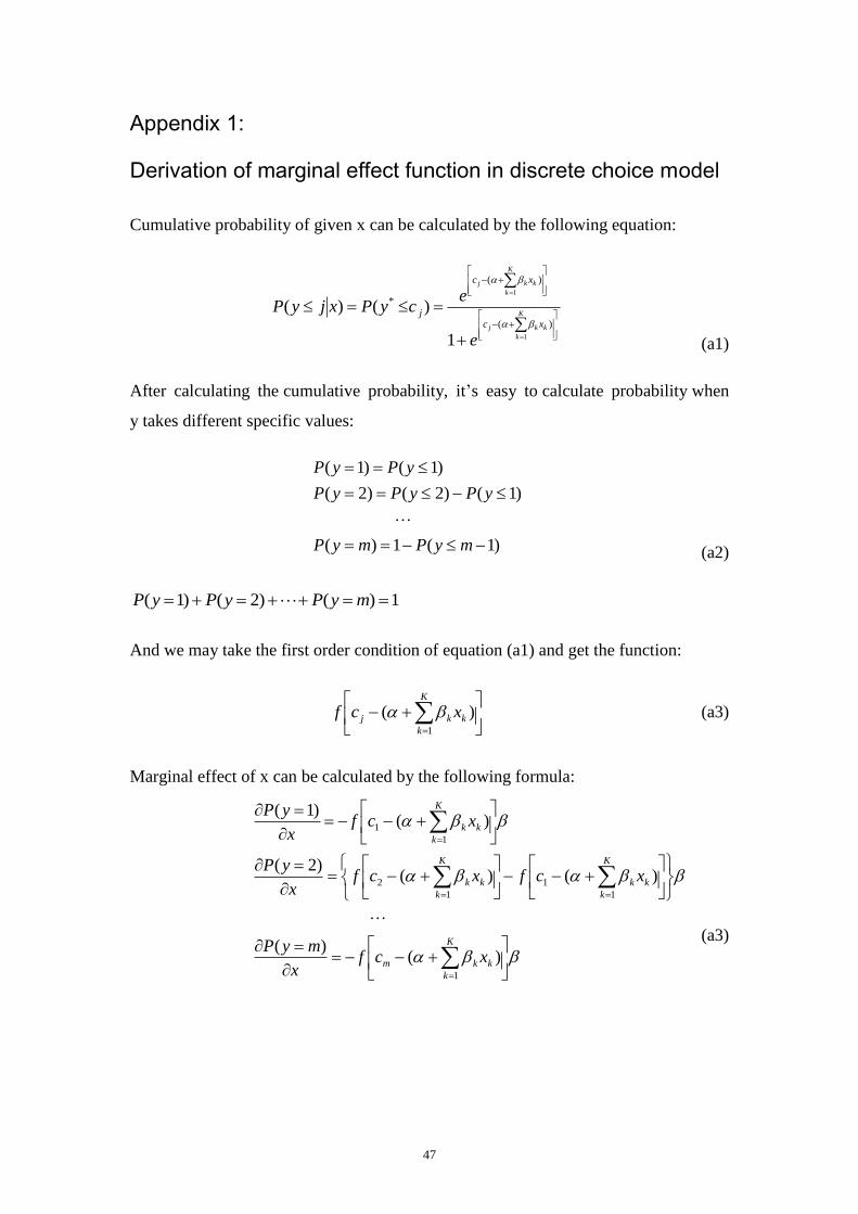
Appendix 1:

Derivation of marginal effect function in discrete choice model

Cumulative probability of given x can be calculated by the following equation:

)(

)(

*

1

1

1

)()(K

k

kkj

K

k

kkj

xc

xc

j

e

ecyPxjyP

(a1)

After calculating the cumulative probability, it‟s easy to calculate probability when

y takes different specific values:

)1(1)(

)1()2()2(

)1()1(

myPmyP

yPyPyP

yPyP

(a2)

1)()2()1( myPyPyP

And we may take the first order condition of equation (a1) and get the function:

)(1

K

k

kkj xcf (a3)

Marginal effect of x can be calculated by the following formula:

)()(

)()()2(

)()1(

1

1

1

1

2

1

1

K

k

kkm

K

k

kk

K

k

kk

K

k

kk

xcfx

myP

xcfxcfx

yP

xcfx

yP

(a3)

48

Comparison of different regression specifications

(1) (2) (3) (4) (5) (6)

income/1000 0.016***

(7.28) 0.019***

(7.34) —

0.016*** (6.16)

0.019*** (5.87)

0.021*** (7.12)

income2 — -1.90e-5***

(-5.93) —

-1.52e-05*** (-4.21)

-1.64 e -05*** (-4.12)

-1.37 e-05*** (-3.08)

relative income/1000 — — 0.027*** (10.93)

— — —

gender -0.112** (-2.27)

-0.069* (-1.78)

-0.071 (-1.04)

-0.083** (-2.09)

-0.084** (-1.99)

-0.084* (-1.89)

age -0.092***

(-8.98) -0.091***

(-8.35) -0.090***

(-8.97) -0.090***

(-7.94) -0.089***

(-8.70) -0.091***

(-8.76)

age2 0.001***

(9.12) 0.001***

(7.97) 0.001***

(7.90) 0.001***

(8.75) 0.001***

(9.14) 0.001***

(8.37)

health -0.363*** (-20.74)

-0.366*** (-20.49)

-0.359*** (-20.36)

-0.352*** (-19.84)

-0.350*** (-19.73)

-0.349*** (-19.11)

marital status (reference group is single)

married 0.921***

(9.23) 0.974***

(9.46) 0.984***

(9.94) 0.998***

(9.43) 0.988***

(9.07) 0.978*** (10.05)

divorced -0.348* (-1.73)

-0.306 (-1.08)

-0.306* (-1.70)

-0.294* (-1.82)

-0.284 (-1.54)

-0.302* (-1.86)

widowed -0.023 (-0.14)

0.031 (0.19)

0.061 (0.39)

0.116 (0.77)

0.118 (0.76)

0.108 (0.69)

employment (reference group is unemployed)

employed 0.335***

(3.25) 0.378***

(3.93) 0.334***

(3.22) 0.270***

(3.10) 0.249***

(2.74) 0.253***

(2.95)

retired 0.534***

(4.86) 0.552***

(4.70) 0.494***

(4.78) 0.326***

(2.62) 0.325***

(2.99) 0.316***

(3.08)

learning 0.521***

(3.99) 0.489***

(4.11) 0.493***

(3.72) 0.507***

(4.16) 0.490***

(4.10) 0.471***

(3.56)

education 0.419***

(4.53) 0.465***

(5.90) 0.367***

(3.66) 0.295***

(3.82) 0.299***

(3.89) 0.292***

(3.28)

urban/suburb 0.078 (1.02)

0.100 (1.55)

-0.019 (-0.29)

0.184 (1.06)

0.094 (0.58)

-0.114 (-0.69)

communication 0.587*** (18.35)

0.586*** (19.52)

0.579*** (19.88)

0.566*** (17.29)

0.562*** (17.84)

0.557*** (17.52)

GDP per capita — — — 0.001 (0.02)

0.021 (0.59)

0.04 (-0.95)

GDP growth rate — — — — 0.054***

(8.79) 0.055***

(9.05)

Gini coefficient — — — — — -0.959***

(-2.90)

Pseudo R2 0.078 0.079 0.082 0.092 0.097 0.097

Number of samples 9328

Appendix 2: