China’s Income Distribution and Inequality

Ximing Wu* and Jeffrey M. Perloff**

January 2004

* Department of Economics, University of Guelph; xiwu@uoguelph.ca. ** Department of Agricultural and Resource Economics, University of California, Berkeley;

member of the Giannini Foundation; perloff@are.berkeley.edu.

ublicly available e examine rural,

timating the entire ine trends in

ased substantially gregate inequality,

the growing gap all inequality

increasingly important role in recent years. In contrast, only the growth of inequality within rural and urban areas is responsible for the increase in inequality in the United States, where the overall inequality is close to that of China. As a robustness check, we show that consumption inequality (which may be a proxy for permanent income inequality) in urban areas also rose considerably.

Abstract

We use a new method to estimate China’s income distributions using pinterval summary statistics from China’s largest national household survey. Wurban, and overall income distributions for each year from 1985-2001. By esdistributions, we can show how the distributions change directly as well as examtraditional welfare indices such as the Gini. We find that inequality has increin both rural and urban areas. Using an inter-temporal decomposition of agwe determine that increases in inequality within the rural and urban sectors andin rural and urban incomes have been equally responsible for the growth in overover the last two decades. However, the rural-urban income gap has played an

Table of Contents

1

auses of Increased Inequality 3

5

4. Maximum Entropy Density Estimation with Grouped Data 7

uality over Time 10

ity 10

erature 13

15

Examine Distributions Directly 16

te Inequality 18

ion and Inequality 18

position of Aggregate Inequality 20

Comparison with the United States 24

7. Consumption Inequality 24

8. Summary 26

1. Introduction

2. C

3. Data

5. Rural and Urban Ineq

Traditional Measures of Inequal

Comparison with the Lit

Distributional Impact of Income Growth

6. Decomposition of Aggrega

Aggregate Distribut

Decom

Increasing Chinese Income Inequality Due to a Growing Rural-Urban Income Gap

1. I

ped summary statistics,

we show that Chinese income inequality rose substantially from 1985 to 2001 because of

increases in inequality within urban and rural areas and the widening rural-urban income gap.

he economy and a

rtionately favored the

ich. We also show that the rural and urban income distributions have

evolved along separate paths, and this divergence has contributed markedly to the rise in the

overall level of inequality.

ncreased rapidly

e because of the

ramall, 2001). The

Chinese government provides Gini indices for only a few, random years using unspecified data

sources, income definitions, and methodologies, hence its inequality measures may not be

tabase).

income

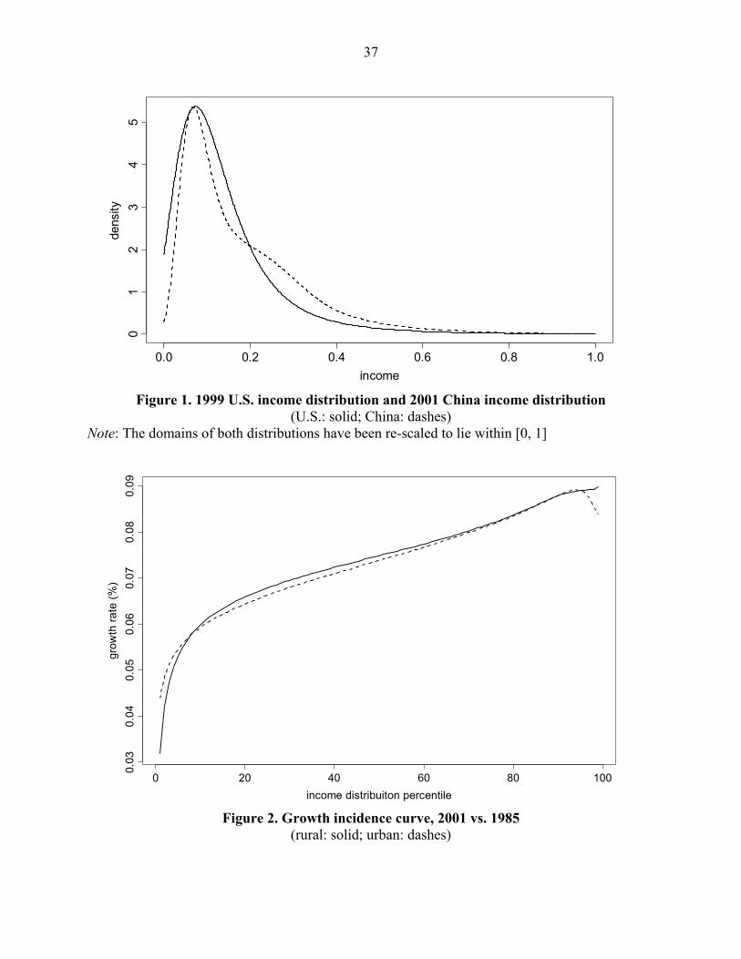
the same Gini value

may have different shapes. As we demonstrate below, although the Gini index of the 1999 U.S.

income distribution (0.414) is almost identical to that of 2001 China income distribution (0.415),

the shapes of the two distributions differ markedly. Thus, welfare implication from comparing

Gini coefficients (or other summary statistics) may be ambiguous. Consequently, we report

ntroduction

Using a new technique to estimate income distributions from grou

We find that China’s dramatic economic growth—a five-fold increase in t

four-fold increase in per capita income since the early 1980s—has dispropo

urban areas and the r

Although a few articles have reported that income inequality in China i

over the last two decades, none shows by exactly how much inequality ros

absence of consistent, reliable income distribution estimates over time (B

directly comparable over time (see United Nations, World Income Inequality Da

Moreover, the Gini index only reflects some aspects of the underlying

distribution: A large amount of information is lost. Two Lorenz curves with

2

several summary statistics as well as reliable estimates of the entire income distribution.

strate that, though

ntly have similar Gini indexes, the reasons these countries are experiencing

gro

This paper makes four contributions. First, we use the new method introduced in Wu and

Perloff (2003) to estimate flexible income distribution functions when summary statistics are

come summary

urban and

ese estimated

income distributions, we provide the first intertemporally-comparable series of income inequality

estimates of China based on a single consistent data source, methodology, and set of definitions.

ributions evolved

n arbitrarily chosen summary statistic, such as the Gini, changed.

We paths. We

is the area under

both density functions: the intersection.

Third, we decompose China’s total inequality between rural and urban sectors to explore

ion over time.

widened rural-urban

income gap, and the shift of populations between these two areas were responsible for the rise in

aggregate inequality. We show that the widening rural-urban income gap played a major role in

China unlike in the United States even though both countries have roughly equal levels of overall

income inequality. Migration from rural to urban areas has little effects on the aggregate

Throughout our paper, we compare Chinese to U.S. income distributions to illu

both countries curre

wing inequality differ.

only available by intervals rather than for the entire distribution. Using the in

statistics based on China’s annual national household survey, we estimate rural,

overall income distributions for each year from 1985 through 2001. Based on th

Second, we show how the rural, urban, and overall Chinese income dist

over time, and not merely how a

show that the rural and urban income distributions evolved along different

employ a simple new measure of the overlap between two distributions, which

the distributional impacts of income growth, rural-urban income gap, and migrat

We show that the rising inequality within both rural and urban areas, the

3

inequality in both countries for different reasons. U.S. migration does not affect inequality

e Chinese migration affects both within and

betw

ality for urban areas.

Consumption is a relatively reliable proxy for permanent income. As such, it provides an

alternative to the limited income data. We find that the consumption inequality is also rising

l inequality. The

ur method to

estimate maximum entropy densities using grouped data. The fifth section estimates China’s

income distributions and inequality for 1985-2001. The sixth section shows the relationship

between total inequality and rural and urban inequality. The seventh section presents measures

of consumption inequality for urban areas as a proxy for permanent income inequality. The last

2. Causes of Increased Inequality

The existing literature (Khan and Riskin 1998, Gustafsson and Li 1999, Yang 1999, Li

n China over the

rates.

We will present evidence that the increase in China’s overall inequality is due to

increases in within inequality, the inequality within the rural sector and within the urban sector,

and between inequality, the inequality due to differences in the average income level between the

rural and urban sectors, as well as population shifts between the sectors. Our explanation is a

within either sector or between the two sectors; whil

een inequality significantly, but these effects are offsetting.

Fourth, as a robustness check, we examine the consumption inequ

rapidly in China.

Section 2 discusses possible causes for the increase in China’s overal

following section describes the available data. The fourth section presents o

section summarizes our results and presents conclusions.

2000, and Meng 2003) argues that income inequality has increased markedly i

last couple of decades. Khan and Riskin (1998) and Li (2000) also provide limited evidence that

China’s rural and urban income inequality differ and are growing at different

4

generalization of two popular explanations—the Kuznets curve hypothesis and the structural

hyp

ing the evolution of total

n within

inequality in each sector, then overall inequality will initially rise as people move from the low-

income (rural) sector to the high-income (urban) sector. Later, inequality will fall, as most of the

d U-shape relationship

ypothesis is true, the

incr may be a

transitory process, and inequality will decline at the conclusion of the urbanization process.

A similar explanation starts from the same premise that the rural-urban income gap is the

driving force for increased overall inequality, but holds that the adjustments described by

structure of China.

te rural and urban

ban areas but

China’s strict residence registration system usually prevents them from obtaining urban

residence status (and hence access to welfare benefits and subsidies enjoyed by urban residents

etween” analysis

e that increases in

rural–urban income differentials is the major cause of rising overall aggregate inequality in

othesis—which have contrasting implications about future inequality.

Kuznets (1955) stressed the role of between inequality in explain

inequality over time. He hypothesized that, if between inequality is greater tha

population settles in the high-income, urban sector. The resulting inverte

between inequality and the income level is called a Kuznets curve.1 If this h

ease in inequality in developing countries during the course of urbanization

Kuznets will not occur due to the secular demographic and institutional

According to this explanation, China’s population has been divided into separa

economies. To a limited degree, migrants from rural areas may seek jobs in ur

and higher paying jobs). For example, Yang (1999) uses a static “within and b

of household survey data from two provinces for 1986, 1992, and 1994 to argu

1 Many studies have estimated the Kuznets curve using cross-country comparisons. Recently this literature has been criticized for failing to account for country-specific effects and for using data that are not comparable. Analyses using panel data from a single country suggest that there is no intrinsic tradeoff between long-run aggregate economic growth and overall equality. See Bruno et al. (1996) for a review of this literature.

5

China.2 He suggests that urban-biased policies and institutions are responsible for the long-term

ease in disparity. If barriers to migration remain, then

ineq

primary cause of

increasing aggregate inequality. This factor is certainly part of the explanation for growing

inequality. However, the complete story is more complex. We will present evidence that, over

ted substantially

ase in overall

ges in within and

between inequality were equally responsible for the increase in overall inequality (in contrast to

the traditional static analysis which concludes that between inequality was largely responsible).

argues that “… a

omote the growth of

widen the

sector may not be able to absorb the large rural

us workers (150 million according to Chang, 2002) and China’s residence registration

system may restraint migration into urban areas. Therefore it is likely that China will maintain a

high level of income inequality for an extended period.

We rely on the largest, most representative survey of Chinese households. The State

Statistics Bureau of China (SSB) conducts large-scale annual household surveys in rural and

rural–urban divide and the recent incr

uality is unlikely to diminish in the future.

Thus, both of these hypotheses emphasize the rural-urban gap as the

the last two decades, the increase in both within and between inequality contribu

to increased aggregate inequality and that population shifts also affect the incre

inequality. In particular, we show that if one takes into account migration, chan

Income inequality does not have a clear secular trend. Chang (2002)

cure for this problem is to accelerate urbanization in the short run and to pr

the urban sector in the long run. Yet, these policies in the short run may further

measured income gap.” However, the urban

surpl

3. Data

2 Because Yang’s analysis is restricted to only two provinces for a shorter time period, his results are not directly comparable to our results.

6

urban areas. The surveys cover all 30 provinces. They usually include 30,000 to 40,000

a two-tier stratified

ach household

ouseholds rotate

out of the sample and are replaced by incoming households. Households are required to keep a

record of their income and expenditure.

rom the SSB survey for

ributions using

summary

statistics for the entire sample, but only for various income intervals. These interval summary

statistics are published for urban and rural areas in the Chinese Statistics Yearbook (“Yearbook”

hen ble income. Our

ide consistent data over

l and urban areas.

Rural income distribution is divided into a fixed number of intervals. The limits for these

income intervals and the share of families within each interval are reported, as is the average

The Yearbooks

report 12 rural income intervals for 1985–1994, 11 for 1996, and 20 for 1995 and 1997–2001.

For urban areas, the Yearbooks report the conditional mean of the 0-5th, 5-10th, 10-20th, 20-40th,

40-60th, 60-80th, 80-90th, and 90-100th percentiles of the income distribution, but not the limits of

these income intervals. We use these publicly available grouped data to estimate the underlying

households in urban areas and 60,000 to 70,000 in rural areas. The SSB uses

sampling scheme to draw a representative random sample of the population. E

remains in the survey for three consecutive years. Each year, one-third of the h

Because we do not have access to the underlying individual data f

all regions and all years, we estimate the Chinese rural and urban income dist

publicly available summary statistics. Unfortunately, the SSB does not provide

ceforth). The Yearbook defines the family income as annual family disposa

sample covers 1985 through 2001, a period for which the Yearbooks prov

time.

The Yearbooks summarize the income distributions differently for rura

income of the entire distribution, but not the conditional mean of each interval.

7

distributions and draw inequality inferences from estimated income distributions. Both rural and

urban income are deflated by the corresponding Consumer Price Index (CPI) from the Yearbook.

4. M

ani and Podder 1976,

and Chen et al. 1991) estimated inequality and poverty using grouped data. These papers

concentrated on estimating the Lorenz curve and its associated inequality indices. In contrast we

tional maximum

ion using grouped data. ;

By dices, we can

examine how the shape of the entire income distribution and how it changes over time.

The principle of maximum entropy (Jaynes, 1957) is a general method to assign values to

ibutions on the basis of partial information. This principle states that one should

choose the probability distribution, consistent with given constraints, that maximizes Shannon’s

aximizing Shannon’s

information entropy

dx

subject to K known moment conditions for the entire range of the distribution

aximum Entropy Density Estimation with Grouped Data

Many earlier studies (e.g., Gastwirth and Glauberman 1976, Kakw

use the method developed in Wu and Perloff (2003) that generalizes the tradi

entropy density method to estimate a very general income density funct

so doing, in addition to determining the Lorenz curve and various welfare in

probability distr

entropy. Traditionally, this maxent density can be obtained by m

( ) ( )logW p x p x= −∫

( )( ) ( )

1,

1,2,..., .i i

p x dx

g x p x dx i Kµ

=

= , =

∫∫

We can solve this optimization problem using Lagrange’s method, which leads to a

unique global maximum entropy (Zellner and Highfield, 1988; Ormoneit and White, 1999; and

Wu, 2003). The solution takes the form

8

( ) ( )0expK

i ip x gλ λ = − −

∑ x1i=

where λi is the Lagrange multiplier for the ith moment constraint. This maximum

method is equivalent to a maximum likelihood approach where the likelihood

over the exponential distribution and therefore con

,

entropy

function is defined

sistent and efficient. See Golan and Judge

(1996) for a discussion of how these two approaches are dual.

subject to simple

haracterizing moments” henceforth. These

cha tire distribution

When only grouped summary statistics are reported, we can estimate the maxent density

by incorporating the grouped information as partial moments. Suppose that, for a certain

distribution, we only know the grouped sum h l limits

[l0, l1, …, lM], and J conditional moments of each interval

All the best-known distributions can be described as maxent densities

moment constraints, which we will call “c

racterizing moments are sufficient statistics for exponential families; the en

can be summarized by the characterizing moments.

mary statistics of M intervals, wit interva

2 1

21 2 2 2

1 2

M

J M JJ

νν ν ν

ν ν ν

, ,

,, , , ,,

1 1 1Mν ν ,

111M

mmν ,=

=∑

(1)

where νm,1 is the share of the mth interval, and . We define the jth partial moment of

a distribution p(x) over the mth interval as

( ) ( )1

1 and 1m

m

l

m j jlf x p x dx m … M j … Jν

−, = , = , ,∫ = , , .

9

Given the underlying density function is ( ) ( )0exp i i1

K

i

p x gλ λ = − −

∑ x , we calculate p(x)

3 ent conditions, we

s, one for each entry of matrix (1). We can solve for the

Lagrange multipliers by iteratively updating

=

using the partial moment conditions. Substituting p(x) into the partial mom

obtain a system of (M × J) equation

( ) ( ) ( ) 11 0λ λ− ′′= + ,G bG G

with ( ) ( )mlb f x p x dxν= − ∫ . The (1m

m j m j jl −, , M × J) by J matrix G consists of M submatrices G(m)

(J × J) stacked on top of one another, where

ore complicated

because we do not know over which ranges the conditional means should be evaluated. For

example in the Yearbooks, unlike rural areas, onl rban

income interval are reported. The moment constraints take the form

( ) ( ) ( ) ( )1

1m

m

lmG g x g x p x dx i j J−

= , ≤ , ≤ .∫

When the interval limits are unknown, the estimation procedure is m

ij j kl

y the share and conditional mean of each u

( )

( )

( ) ( )1

2

1

1 ,m

m

lm l

p x dx m … M

xp x dx m … M

ν

ν−

,

,

= , = ,

= , =

∫

∫

( )

( )

11

m

m

lm l −

, ,

, ,

(2)

known density function, p(x). Wu and

Perloff (2003) show how to estimate the location of these limits using a Quasi-Newton’s method,

jointly with the density function.

where the interval limits lm( )’s are functions of the un

3 In general, the functional form p(x) is unknown. Wu and Perloff (2003) discuss choosing a model using bootstrapped Kullback-Leibler Information Criterion.

10

Because we do not have individual Chinese data corresponding to the reported grouped

ing raw income

See the Appendix

tial updating method of mo lection described

information, we cannot directly examine the effectiveness of the proposed method using Chinese

data. Nonetheless, we demonstrate the effectiveness of the proposed method us

data from the 2000 U.S. Current Population Survey (CPS) March Supplement:

and Wu and Perloff (2003). Using the sequen del se

in Wu and Perloff (2003), we find that the specification ( ) ( )( )0log 1 i

ii

4expp x λ= −∑

the best overall fit according to the bootstrapped Kullback-Leibler Informati

method works extremely well for the U.S. data: The fit is virtually as close as

with moment conditions for the entire sam

x gives

on Criterion. This

could be obtained

ple. For example, given the population shares and

rval limits, the estimated distribution had a Gini of 0.413;

whereas the Gini based on individual data is 0.414.

tributions from

s, we use three

approaches to determine whether inequality rose over the last two decades. First, we examine

how traditional inequality measures changed over time. Second, we examine growth incidence

curves, which trace out the growth rate of each income quantile between two points of time.

Traditional Measures of Inequality

We start by examining three traditional measures of inequality—the Gini Index, the mean

logarithm deviation of income, and comparisons of quantile ranges—for rural and urban areas

separately. We use these measures to examine how inequality has changed over time.

=+

means for 8 intervals but not the inte

5. Rural and Urban Inequality over Time

Using this method, we estimate the Chinese rural and urban income dis

publicly available summary statistics. Based on these estimated distribution

Third, we compare the estimated distributions directly.

11

From the rural survey, we have 12 intervals for 1985–1994, 20 for 1995, 11 for 1996, and

th 5-10th, 10-20th, 20-

ibution, but not the

ubject to the

proportion of families in each known interval. Because the limits for the income intervals are

unknown for urban income, we estimate them jointly with the density function. Again, we find

that the specification

20 for 1997–2001. For urban areas, we have conditional means of the 0-5 ,

40th, 40-60th, 60-80th, 80-90th, and 90-100th percentiles of the income distr

limits of these income intervals.4 We estimate the rural income distribution s

4 i( ) ( )( )exp log 1p x xλ= − +∑ 0 ii=

according to the bootstrapped Kullback-Leibler Information Criterion.

Table 1 shows how our various inequality measures for each year in

first two columns of numbers report the Gini index for rural and urba

( )log / iix

nµ∑

gives the best overall fit for both areas

our samples. The

n areas based on our

esti ral and urban mean

logarithm deviations (MLD =

mated distributions for each year. The next two columns show the ru

1 , where n is the number of people).5

urban areas

es their

According to both measures, rural areas have greater inequality than

throughout the period. On average, the rural Gini is 1.4 times and the MLD is 2.2 tim

urban counterparts.

ncome distribution estimate than our urban one because the ls (20 versus 8), spans the

nd has income lim , the top urban he high end of the

decile during our sample period, we cannot recover this increase without further information. 5 The MLD belongs to the family of generalized entropy index, Ia =

, where a ≥ 0. A low value of a indicates a high degree of

e can show that

4 Consequently, we have more confidence in our rural i rural distribution is summarized in more interva

entire distribution relatively evenly, a its. More importantlyinterval covers the entire 90-100th decile. If most of the dispersion at tdistribution occurred within the top

( / ) 1 /[ ( 1)]ai

ix na aµ − − ∑

“inequality aversion”. On ( )10lim log /a a in i

I xµ→ = ∑ , which is the MLD. In this study, we focus on the MLD as it gives the simplest formula for the intertemporal decomposition of inequality (see Section 5).

12

The correlation between the Gini and the MLD is 0.76 for rural areas and 0.73 for rural

er the sample

re confident that

renz curves from

the estimated densities. For example, the 1985 Lorenz curves of rural and urban distributions lie

above those for 2001 everywhere, suggesting that the 1985 distributions Lorenz dominate those

6

at the low end of

m 0.127 to 0.213. Urban inequality rose faster, though

it remained below that in rural areas. The urban Gini increased by 40.8% from 0.191 to 0.269,

and the MLD nearly doubled from 0.060 to 0.119.

Another traditional approach to assess the changes in inequality is to compare quantile

ation loss for

of the entire range,

t four columns of

Table 1 show the estimated 90/50 and 50/10 quantile ratios. If Q(p) is the p percentile, then the

90/50 quantile ratio is Q(90)/Q(50). The 90/50 ratio reflects the relative shares of a wealthy

group to the average group. Similarly, the 50/10 quantile ratio shows the relative shares of the

average to a poor group. For rural and urban areas, both measures increased by between 20 and

25% during the sample period. Although not shown in the table, the 90/10 ratio increased by

around 50%. The similarity in changes of these quantile ratios suggests that the different

areas. Both inequality measures for rural and urban areas increased steadily ov

period. The rural Gini increased by 26% from 0.272 to 0.343. One reason we a

the Gini is capturing a real, upward trend is that we compared the calculated Lo

for 2001.

The rural MLD—which places a relatively large weight on the income

the distribution—increased by 67.7% fro

ranges. Because of the interval summary statistics nature of our data, the inform

quantile estimates due to grouping may be less than that of inequality index

which suffers from the aggregating over the top and bottom quantiles. The las

th

6 Given the estimated density f and sample average µ , the Lorenz curve is obtained

numerically as ( ) ( )1

0

1L p xf x dxµ

−

= ∫( )F p

, where 1F − is the inverted distribution function.

13

inequality increase rate, as measured by Gini and MLD, is likely due to the difference in

evo

n any Chinese

countries. As

migrants from rural who work urban areas usually cannot obtain urban residence status, they are

excluded from urban household surveys. Because migrants can only obtain jobs that pay less

unted as urban

ral standards,

including them in the rural household surveys raises rural income inequality. Moreover, Schultz

(2003) notes that restrictions on permanent migration reduce the returns that rural youth can

expect to realize through profitably moving to a higher wage labor market. Consequently, the

household registration system increases the gap in investments in education between rural and

Comparison with the Literature

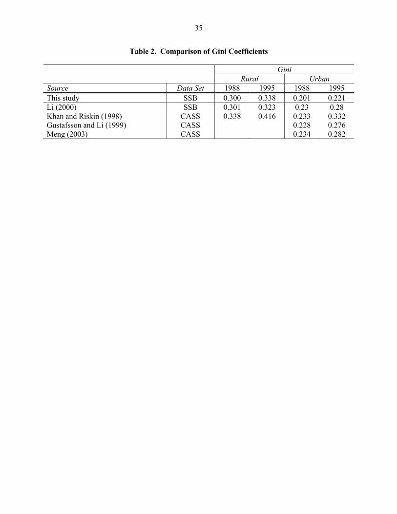
We can compare our estimates to those from four previous studies. As these other studies

ini indexes for only

those years.

for 1988 and 1995.

Our estimates of the rural Gini of 0.300 in 1988 and 0.338 in 1995 are close to Li’s (2000)

estimates based on SSB data of 0.301 and 0.332. Our estimates of the urban Gini of 0.201 in

lutions of the upper and lower tails of the distributions.

Given how China records rural migrants to urban areas, studies based o

data set measure rural and urban inequality differently than they would in other

than those of other urban workers and because the number of migrants grew considerably during

the sample period, urban inequality measures are lower than if migrants were co

residents.7 On the other hand, if migrants earn relatively high incomes by ru

urban families and the rural-urban gap in the long run.

only report the Gini for a few years, Table 2 compares the rural and urban G

Li (2000) reports rural and urban Gini index based on SSB micro data

7 During the sample period, the share of the rural population fell from 76% to 62%. The number of migrant workers is estimated to be around 80 million in the mid-1990s. See Bramall (2001) and references therein.

14

1988 and 0.221 in 1995 are not quite as close to Li’s estimates, 0.23 and 0.28. As we discussed

n from excessive

rban income distribution is summarized by only 8 groups and

the

Because the SSB household survey data are not publicly available, the other three

studies—Khan and Riskin (1998), Gustafsson and Li (1999), and Meng (2003)—use data from

Chinese

roader definition of

e than does the SSB. Although three of these studies use the CASS data, their estimates of

the Gini differ, because they make different assumptions about the underlying data (Bramall,

2001).

Khan and Riskin (1998) report higher rural inequality measures based on CASS data than

ut their estimates of the 1995 value range from 0.28

to 0 those of all four

previous studies. The lower value of our estimates may be due to difference in the underlying

data sources, definitions of income, or methodology.

Nonetheless, all studies report that rural and urban inequality increased from 1988 to

.282 in 1995 to

0.313 for 1999 based on a CASS survey covering six provinces.

above, underestimates of urban inequality may be the result of lost informatio

grouping and top coding as the u

highest interval covers the top decile.

smaller, less representative surveys conducted by the Economics Institute of the

Academy of Social Sciences (CASS) in 1988 and 1995.8 The CASS uses a b

incom

either we or Li (2000) do based on SSB data. All three CASS studies estimate the 1988 urban

Gini at 0.23 (above our estimate of 0.20), b

.33 (all higher than our 0.22). Thus, our urban estimates are lower than

1995. In addition, Meng (2003) reports that the urban Gini increased from 0

8 Unlike the SSB survey that covers all 30 provinces, the CASS survey covered 28 provinces for rural areas and 19 provinces for urban areas in 1988, and 10 provinces for rural areas and 11 provinces for urban areas in 1995.

15

Distributional Impact of Income Growth

ged. The main

pend on the choice

of the index because indices differ in the weight they place on various portions of the income

distribution (Atkinson, 1970). We need to know how the entire distribution shifted to determine

ffects the

distributions over time, we use the ratio of income corresponding to the same percentile of two

distributions. Following Gastwirth (1971) and Ravallion and Chen (2002), we invert the CDF at

the p quantile to obtain the corresponding income

Although these inequality measures indicate that inequality increased significantly during

the sample period, these indices do not fully describe how the distribution chan

problem with using only inequality indices is that the welfare implications de

the full social welfare effects.

During the sample period, the average real income more than doubled in rural areas and

increased by 169% in urban areas. To examine how this rapid income growth a

th

t

( ) ( )1 0 1Q p F L p pµ− ′= = , ≤ ≤ ,

where F is the cumulative distribution function, L’(p) is the slope of the Lorenz curve at the pth

quantile, and µ is the overall average income. The growth incidence curve (GIC) between time

t–1 and time is

( ) ( )1 1 1

( )GIC 1 1 0 1.( )

t t t

t t t

L p Q pp pL p Q p

µ

− − −

′= − = − , ≤ ≤

( ) µ′

It traces out the growth rate of each income quantile between t-1 and t.

If the Lorenz curves do not change during this period, the GIC is equal to the average

growth rate (µt/µt-1) everywhere so that growth is neutral. The growth is said to be pro-rich if the

GIC is upward sloping and pro-poor if the GIC slopes down. If the GIC is everywhere above

16

zero, then the distribution of time t Lorenz dominates that of time t–1. In other words, the

Lor one.

poorest rural group

grew slightly slower, but that of the middle rural group grew slightly faster. The ratio is

everywhere above zero, so all income groups benefited in absolute terms. The rich grew

onately richer during this period, as the curves are almost everywhere increasing.9 For

rura or the richest is

We note that the annual average and median growth rates for both sectors are about 7.4%.

Thus, the estimated growth rates based on summary statistics of micro household surveys agree

with the government number of per capita GDP growth during this period, which is about 7% to

8%.

Although it provides a straightforward way to examine changes in the distributions over

time, the GIC only reflects certain aspects of the evolutionary process. For example, the GIC

analysis does not show how the general shape of the income distribution changed over time. Is

the increased inequality as measured by the Gini or MLD caused by a rightward shift of the mode,

become bi-modal

due to “hollowing out” of the middle class? For further insight into this process, we examine the

enz curve of the second distribution lies strictly above that of the first

Figure 2 plots the GIC between 1985 and 2001, divided by the number of years in

between, for both areas. Compared with urban areas, the incomes of the

proporti

l areas, the annual growth rate for the poorest group is about 3%, while that f

nearly 9%.

Examine Distributions Directly

a thickened tail, or some other more complex change? Does the distribution

9 The bent-down section at the high end of the urban distribution may be due to top-coding in survey of the highest income group and under-reporting of their income by the rich. Both of these effects are presumably more important in the richer urban area than in the rural area.

17

shapes of our estimates of the flexible density function, which allows for multi-modal

dist

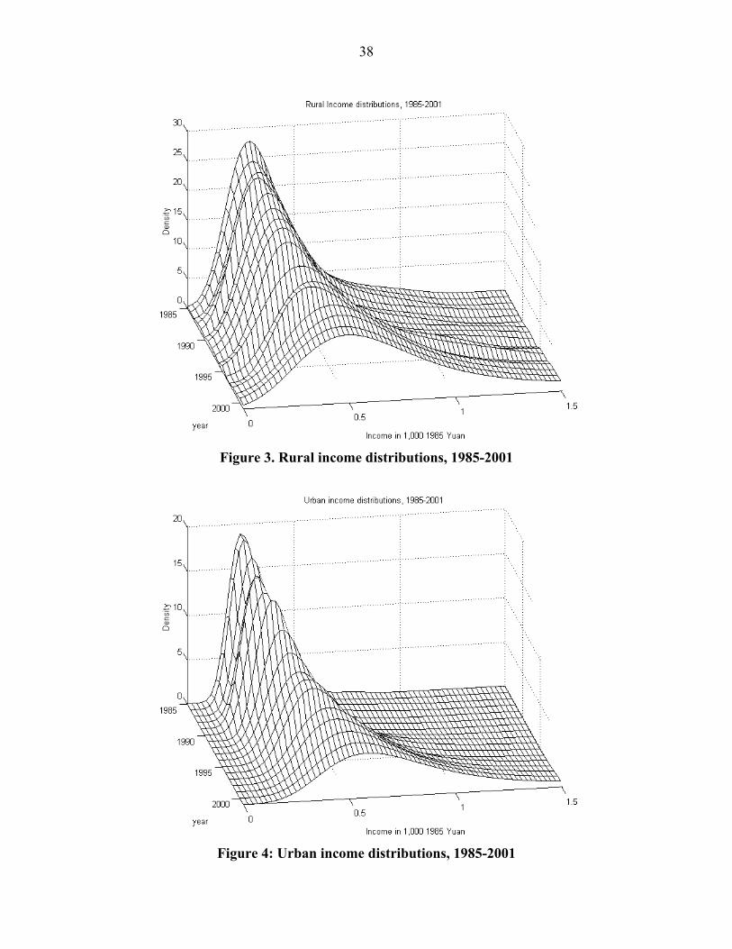
001, and Figure 4

distribution has a

single mode. However, dispersion increased considerably over time, largely because the right

tails grew longer. Moreover, the income distributions gradually but persistently moved to the

righ ng a general increase in

paring

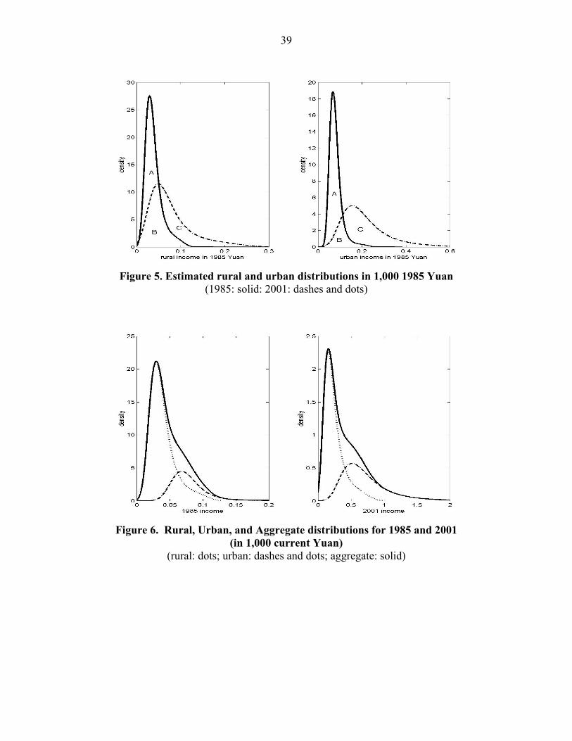
distributions for pairs of years. The left panel of Figure 5 shows that the 2001 rural income

distribution is much more dispersed than the 1985 distribution. The distribution mode rose 68%

from 292 Yuan in 1985 to 490 (in 1985) Yuan in 2001. Despite the rightward shift of the mode,

ode in 2001 is

.86.

) rose more

rapidly than in rural areas (left panel). Moreover, the fraction of households with very low levels

of income fell substantially. The mode of the urban distribution increased by 140% from 681

2001 fell to 25%

of that in 1985. The distribution became more symmetric—skewness decreased from 1.82 to

1.47—reflecting a relative decrease in the share of poor and increase in the share of wealthy

people. The kurtosis fell from 8.28 to 6.05, reflecting the substantial flattening of the peak.

Compared with the rural distribution, the share of people with low absolute income (the height of

ributions.

Figures 3 shows how the rural distribution changed between 1985 and 2

shows the shift in the urban distribution. Throughout the sample period, each

t (and correspondingly, the weight at the mode decreased), reflecti

incomes.

These rightward shifts in the distributions are more clearly seen by com

the skewness increased from 1.28 to 1.39. The height of the distribution at the m

only about 40% of the 1985 peak, which caused kurtosis to fall from 4.95 to 4

The level and the dispersion of the urban income (right panel of Figure 5

Yuan in 1985 to 1,634 in (1985) Yuan in 2001, while the density of the mode in

18

the left tail) was much smaller, which helps to explain why our inequality estimates are lower in

urb oor.

stance or closeness

verlap between

two distributions, the intersection, which is the area under both density functions. This statistic

for two density functions p(x) and q(x) on the real line or its subsets is defined as

an areas, especially for the MLD, which heavily weights the income of the p

By how much did the distributions shift? We can assess the overall di

between two distributions directly. We propose a simple new measure of the o

[ ]min ( ), ( )p x q x dxΩ = ,∫

wh If Ω = 0, then

utions, Ω is higher for rural areas, 0.54, than for urban areas,

0.24, because the urban distribution shifted right by considerably more did the rural one.

in the rural and urban distributions have on overall

stion, we decompose the total Chinese inequality between rural

and tor and between

sectors contributed to the increase of total inequality.

hted mixture of

tribution to calculate the inequality

ose value is equal to area B in Figure 5. 10 It is restricted to lie within [0 1], .

p(x) and q(x) are disjoint. If Ω = 1, then p(x) and q(x) coincide.

For the 1985 and 2001 distrib

6. Decomposition of Aggregate Inequality

What effect do these unequal shifts

inequality? To answer this que

urban areas. Our results suggest that increased inequality within either sec

Aggregate Distribution and Inequality

We compute China’s aggregate income distribution as a population-weig

the rural and urban distributions. We use the resulting dis

10 Compared with another commonly used distance measure such as the Kullback-Leibler distance, [ ]( ) ln ( ) / ( )p x p x q x d∫ x , our measure has three advantages. First, it has an intuitive graphic interpretation as the overlapping areas of two distributions. Second, and more important, it is symmetric in the sense that Ω is invariant to the order of p(x) and q(x): Ωp,q = Ωq,p. Third, this index can be used to compare directly more than two distributions.

19

indices of the aggregate distribution. Denoting rural and urban income distribution as pr(x) and

pu(x tain the aggregate distri e) respectively, we ob bution by taking their weight d sum:

( ) ( ) ( )r r u up x s p x s p x= + ,

where sr and su is the share of rural and urba

(3)

n population. During the sample period, the share of

urban population increases steadily from 24% to 38%.

Figure 6 illustrates the relationship of the aggregate distribution (solid) to the rescaled

l and urban densities

ese two curves

rall shape of the

aggregate distribution was relatively unchanged over the sample period, but the right tail became

thicker (note that the scale of the two diagrams differ). The left tail of the 1981 aggregate

den re not that poor)

density is almost

lumn), which were

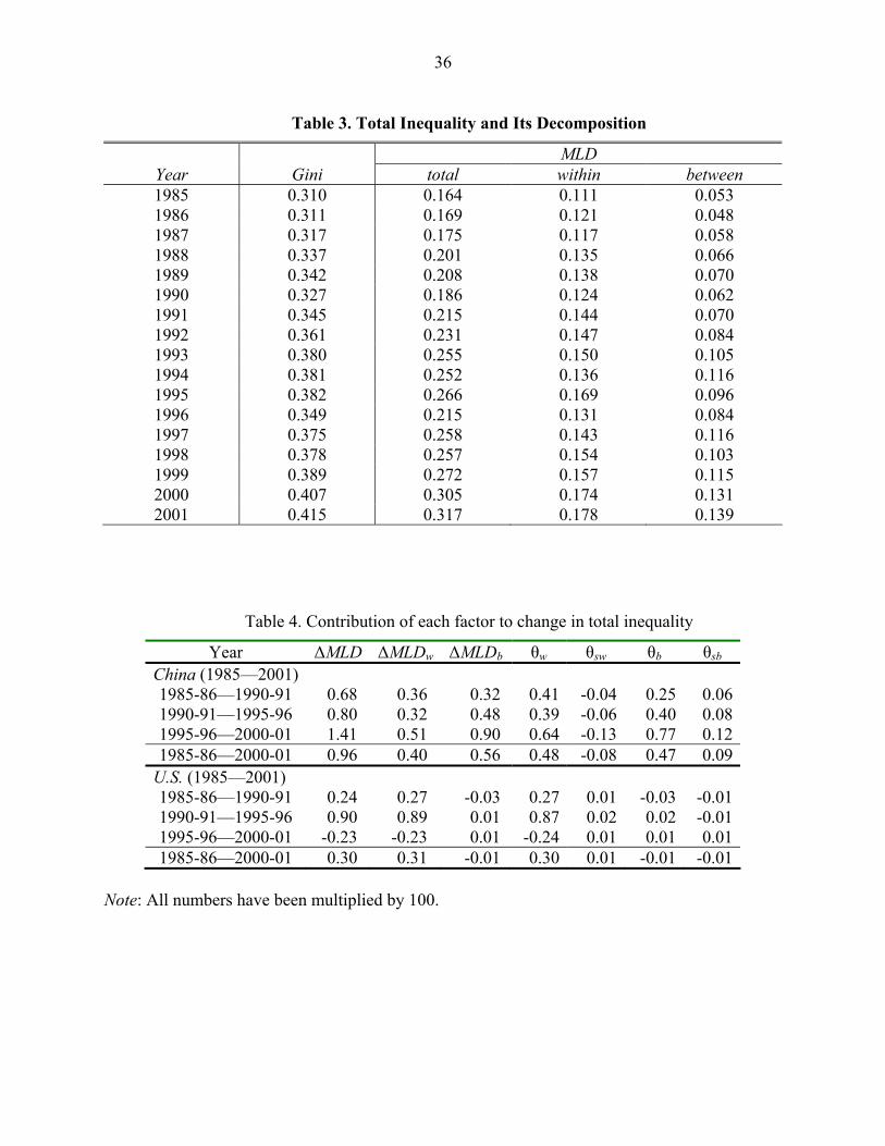
calculated from the estimated aggregate p(x). Over the sample period, the Gini index increased

34% from 0.310 to 0.415, and the MLD nearly doubled from 0.164 to 0.317. The overall

inequality is much higher than either rural or urban inequality because of the substantial rural–

urban income gap. As shown by Equation (3) and Figure 6, the increased aggregate inequality

was due to changes in the rural or urban distributions, their interaction (the degree to which the

two distributions overlap), and the population weights.

rural (dot) and urban (dash-dot) distributions for 1985 and 2001. The rura

are rescaled by their corresponding population weights so that the areas below th

sum to one. By comparing the 1985 and 2001 figures, we see that the ove

sity is almost completely coincident with the rural density (urban dwellers a

while both the rural and urban densities span the right tail. In 2001, the urban

entirely responsible for the right tail of the aggregate density.

Table 3 reports the Gini index (second column) and the MLD (third co

20

Decomposition of Aggregate Inequality

ality and between

can derive the

on. The most

commonly used inequality index, the Gini, is not decomposable in this sense, so generally we

cannot calculate the aggregate Gini index from the Gini indices of its subgroups. However, the

ML and urban MLD’s to derive the aggregate MLD,

and we can show which factors contributed to the growth of the aggregate MLD over time.

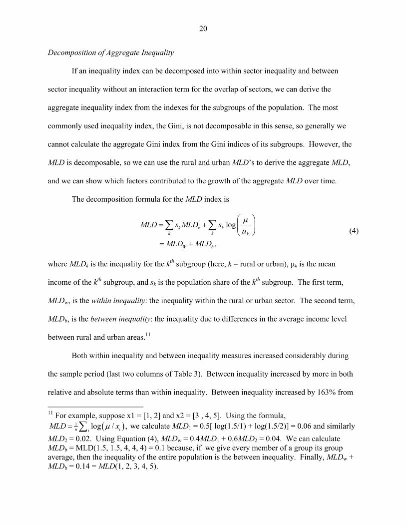
The decomposition formula for the MLD index is

If an inequality index can be decomposed into within sector inequ

sector inequality without an interaction term for the overlap of sectors, we

aggregate inequality index from the indexes for the subgroups of the populati

D is decomposable, so we can use the rural

,

k k k

W bMLD MLDµ

= +

logk k k

MLD s MLD s µ

∑ ∑

where MLDk is the inequality for the k subgroup (here, k = rural or urban), µ

income of the kth subgrou

= + (4)

thk is the mean

p, and sk is the population share of the kth subgroup. The first term,

ML w The second term,

MLDb, is the between inequality: the inequality due to differences in the average income level

between rural and urban areas.11

Both withi erably during

sed by more in both

han within inequality. Between inequality increased by 163% from

D , is the within inequality: the inequality within the rural or urban sector.

n inequality and between inequality measures increased consid

the sample period (last two columns of Table 3). Between inequality increa

relative and absolute terms t

11 For example, suppose x1 = [1, 2] and x2 = [3 , 4, 5]. Using the formula,

( )1 log / ,in iMLD xµ= ∑ we calculate MLD1 = 0.5[ log(1.5/1) + log(1.5/2)] = 0.06 and similarly MLD2 = 0.02. Using Equation (4), MLDw = 0.4MLD1 + 0.6MLD2 = 0.04. We can calculate MLDb = MLD(1.5, 1.5, 4, 4, 4) = 0.1 because, if we give every member of a group its group average, then the inequality of the entire population is the between inequality. Finally, MLDw + MLDb = 0.14 = MLD(1, 2, 3, 4, 5).

21

0.053 to 0.139, while within inequality increased by only 61% from 0.111 to 0.178. As a result

of b

three subperiods.

each two adjacent

years and examine the changes for the entire period and three five-year sub-periods, 1985-86

through 1990-91, 1990-91 through 1995-96, and 1995-96 through 2000-01. The first three

ntire period and

increased from 0.16 to

annual increase over the entire period was 0.01, the annual rate of

increase rose over time, so that the average increase in the third subperiod was more than

doubled that in the first subperiod.

In the first subperiod, the contribution of changes in within (0.36) and between (0.32)

aggregate inequality are roughly equal. However, during the second

and o the within

r about 58%

(≈0.56/0.98) of the total increase.

Equation (4) shows that three factors contribute to total inequality: the inequality within

each subgroup (MLDk), the relative average income of each subgroup (µk/µ), and the population

shares of each subgroup (sk). During the sample period, the share of rural population fell from

ysis does not separate the impact

of changes in population structure from that of changes in the distribution of each sector.

oth of these increases, total MLD inequality more than doubled.

In Table 4, we show inequality increased over the entire period and in

To avoid year-to-year fluctuations, we combine the distribution estimates of

columns of Table 4 report the annual change in aggregate inequality for the e

three subperiods.12 During the sample period, the overall MLD inequality

0.32. Although the average

inequality to the change in

third subperiods, the between inequality’s contribution increased relative t

inequality. For the entire period, the increase in between inequality accounts fo

76% to 62%. However, the simple “within and between” anal

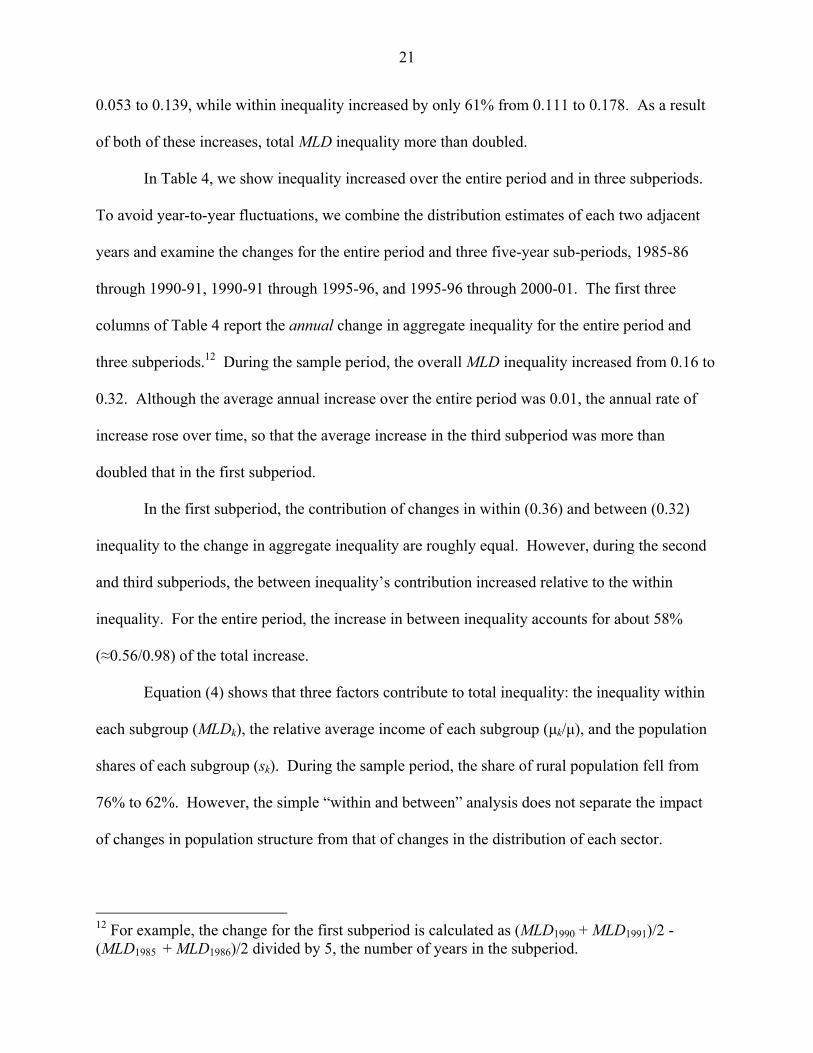
12 For example, the change for the first subperiod is calculated as (MLD1990 + MLD1991)/2 - (MLD1985 + MLD1986)/2 divided by 5, the number of years in the subperiod.

22

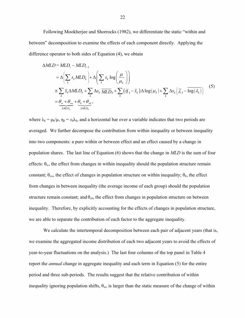
Following Mookherjee and Shorrocks (1982), we differentiate the static “within and

of each component directly. Applying the

difference operator to both sides of Equation (4), we obtain

between” decomposition to examine the effects

( ) ( ) ( )

1=

log

log log

t t

k k kk k k

kk k k k k kk kk k k k

w sw b sb

MLD MLD MLD

s MLD s

s MLD s s sMLD

µµ

µ λη λ

−

∆ −

= ∆ + ∆

≅ ∆ + ∆ + − ∆ + ∆ −

∑ ∑

∑ ∑ ∑ ∑ k

,w bMLD MLD

θ θ θ θ∆ ∆

= + + +

where λk = µk/µ, ηk = skλk, and a horizontal bar over a variable indicates th

averaged. We further decompose the contribution from within inequality or betw

effects: θw, the effect from changes in within inequality should the population

constant; θsw, the effect of changes in population structure on within inequality;

from changes in between inequality (the average income of each gr

(5)

at two periods are

een inequality

into two components: a pure within or between effect and an effect caused by a change in

population shares. The last line of Equation (6) shows that the change in MLD is the sum of four

structure remain

θb, the effect

oup) should the population

structure remain constant; and θsb, the effect from changes in population structure on between

inequality. Therefore, by explicitly accounting for the effects of changes in population structure,

ality.

of adjacent years (that is,

oid the effects of

year-to-year fluctuations on the analysis.) The last four columns of the top panel in Table 4

report the annual change in aggregate inequality and each term in Equation (5) for the entire

period and three sub-periods. The results suggest that the relative contribution of within

inequality ignoring population shifts, θw, is larger than the static measure of the change of within

we are able to separate the contribution of each factor to the aggregate inequ

We calculate the intertemporal decomposition between each pair

we examine the aggregated income distribution of each two adjacent years to av

23

inequality, ∆MLDw = θw + θsw, which includes the effects of the changing population (θsw). That

educes the effect

the entire period, migration partially offsets the effect

of i

In contrast, the contribution of between inequality—the rural-urban income gap—is

smaller when we account for change in population shares. Because of the widening rural-urban

inco 9% (= 0.09/0.47)

ly offsetting (θsw +

θsb = 0.01). Overall, the static “within and between” decomposition underestimates the

contribution of increased within inequality because it fails to take into account the influence of

change in population structure. For the entire period, the change in within and between

pared to 42% and

role; but in recent

years, between inequality contributed more to overall inequality change. After controlling for

the effects of migration, we find that changes in within inequality were responsible for 63% of

the change in total inequality for the late 1980s; the two components were equally important in

the early 1990s; and between inequality played a larger role (55%) in the late 1990s. It is in the

late 1990s that the most dramatic increase in inequality occurs. The annual increase in aggregate

inequality is 0.014 in the MLD, compared with 0.0068 and 0.008 for the first two sub-periods.

is, migration from higher-inequality rural areas to lower-inequality urban areas r

of rising within inequality. On average for

ncreased within inequality by 17% (= -0.08/0.48).

me gap, migration enhances the effect of increased between inequality by 1

on average.

The effects of migration on the within and between inequality are near

inequality each contributes about 50% to the increase in total inequality, com

58% in the simple “within and between” decomposition.

The pattern varies over time. Initially within inequality played a larger

24

Comparison with the United States

regate income

a developing and

e conduct the same

intertemporal between-within analysis using U.S. data: the March Current Population Survey

(CPS) for 1985-2001. We look at the change in inequality for the entire period as well as for

4.

ina is that

overall inequality.

However, China’s growing rural-urban income gap and increasing migration into urban areas

further forces inequality to rise. For the same period, U.S. inequality in both sectors increased

considerably and almost all the changes in overall inequality are attributed to these changes in

pulation (70%)

sidering the

neither between

inequality nor migration has played a significant role in the rise in U.S. overall inequality. With

the share of urban population stable for an extended period, Kuznets’ the migration/urbanization

process appears to have come to a conclusion. However, instead of going down, the overall

ch sector.

7. Consumption Inequality

Because we have been relying on highly aggregate income information, we consider an

alternative approach in which we examine Chinese consumption inequality as a proxy for

permanent income inequality. Consumption data are only available for urban areas, where

Comparing the determinants of changes in Chinese rural, urban, and agg

distributions to those in the United States may illustrate the difference between

an industrial economy with currently similar levels of income inequality. W

three five-year subperiods. The results are reported in the bottom panel of Table

One important effect that is common to both the United States and Ch

inequality is increasing rapidly in both rural and urban areas, which drives up

within inequality. In contrast to the pattern in China, the U.S. share of urban po

and the rural-urban income ratio (75%) have remained relatively constant. Con

relatively small share of rural population and the stable rural-urban income ratio,

inequality has been rising steadily due to the increased inequality within ea

25

consumption information is summarized in the same format as is income distribution by the

Yea

lly on the choice

anent income may

be the preferred indicator of household resource, but it is unobservable. Although measured

income is correlated with permanent income, its substantial transitory component is uncorrelated

old permanent

l to permanent income. Moreover, it exhibits relatively smaller

tran e inferences using

consumption rather than income.

According to several studies of inequalities in the OECD countries report, the recent rise

in income inequality was not accompanied by a similar increase in consumption inequality.

come inequality.

es not apply to China,

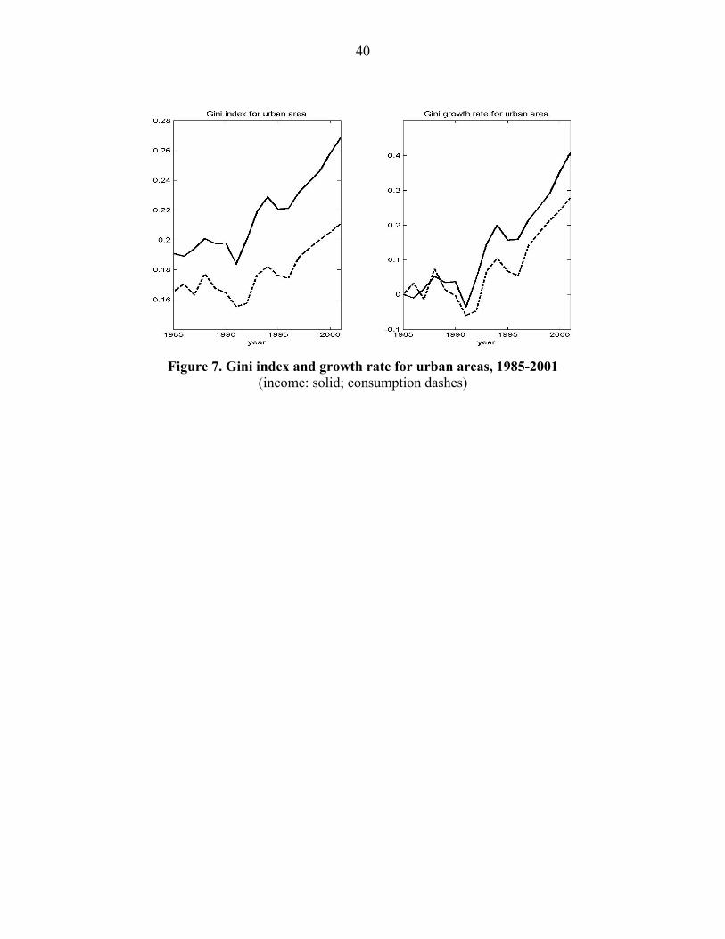
igure 7

compares the estimated Gini index for income and consumption in the left panel and their growth

rate in the right panel. Although consumption inequality is lower than income inequality, its

f the income inequality. In contrast, Krueger and Perri (2002)

report that, although the U.S. income Gini index rose substantially from 0.31 to 0.41 during the

last quarter of the twentieth century, the consumption Gini index rose 2 percentage points from

roughly 0.25 to 0.27. During the 1990s when the income inequality increased considerably, the

consumption inequality actually declined.

rbooks.

Jorgenson (1998) argues that estimates of welfare indices depend critica

between income and consumption as a measure of household resource. Perm

with permanent income. Measured consumption can serve as a proxy for househ

income, if it is proportiona

sitory fluctuation. Therefore, we may be able to make more reliable welfar

These findings are sometimes cited in response to public concern about rising in

Regardless of the validity of this argument in OECD countries, it do

where the income and consumption inequality measures are highly correlated. F

growth rate closely parallels that o

26

Prior to 1997, the ratio of average expenditure to average income for households within

th tion by

rnment subsidies

ive percentiles fell

to 0.96 for 1997–2001, suggesting that the safety net for the poor may not be as effective as it

formerly was. The (relative) deterioration of the consumption of those at the low end of the

lity near the end of

orkers in the state-

ensations.13 The

state public-transfer system failed to provide them with the much-needed “safety net”. China’s

government transfers as a share of GDP decreased from 0.35% in 1985 to 0.28% in 2001. In

contrast, Keane and Prasad (2003) observe that, unlike most other transition countries, Poland

experienced very little increase in overall income inequality. The main reason was that, during

the from about 10% of

8. Summary

from 1985

through 2001. We estimate China’s income distribution using a new maximum entropy density

approach that works well when only a limited set of summary statistics by income interval are

available. The maximum entropy principle is a general method to assign values to probability

distributions on the basis of partial information. We extend this method to grouped data and use

the 0-5 percentiles of the income distribution averaged 1.06. Hence, consump

households with very low income exceeded their income, probably due to gove

for urban residents. However, the consumption–income ratio for the bottom f

income distribution and the subsequent rapid increase in consumption inequa

the sample during the late 1990s may be partially due to the large number of w

owned enterprises who were laid off with only nominal unemployment comp

earlier years of transition, there was a sharp increase in social transfers,

GDP to 20%.

We examine the evolution of China’s income distribution and inequality

13 Reportedly, 11.57 million workers were laidoff in 1997 (China Development Report, 1998).

27

it on summary statistics of income data from annual Chinese household surveys. We are able to

con

ey, we are able to

easures. In contrast

to, most previous studies of Chinese income inequality used an alternative survey that is only

available in a couple of years and that does not cover the entire country.

ban inequality

. Direct

ome distributions

are shifting to the right over time. The overall dispersion increased considerably, due in large

part to the growth of the right tail of the distribution and the failure of the share of the very poor

to decline significantly. Although most people’s incomes rose over time, the rapid income

income than did

ural-urban income gap, and

shifts of population between urban and rural areas combined to drive up the aggregate inequality

substantially. In contrast to previous studies that used static decompositions that attributed the

growth in overall inequality largely to increases in the rural-urban gap, our dynamic

decomposition shows that the increase in within and between inequality contributed equally to

the rise in overall inequality over the last two decades. We do find, however, that the rural-

income gap has played an increasingly important role in recent years.

firm that this new method works extremely well on U.S. data.

Using this new technique and data from the most inclusive Chinese surv

provide the first intertemporally consistent estimates of China’s inequality m

We find that rural and urban inequality have increased substantially. Ur

was lower than rural inequality during the sample period, but it is rising faster

examination of the estimated distributions reveals that both rural and urban inc

growth favored the richest members of society, who enjoyed a larger increase in

the poor.

Rising inequality within rural and urban areas, the widening r

28

Finally, we find that consumption inequality, arguably a better indicator of economic

tantially during the sample

per ina.

(comparable to that

in the United States) and rising due to increases in within and between inequality. Currently

rural incomes are less equally distributed than urban incomes. However, urban inequality is

ity will

rural–urban

ple move to urban

areas. Government restrictions limit migration from rural to urban areas. Even if such migration

were permitted, it probably is not possible for the urban economy to accommodate the majority

of the gigantic rural population. Thus, in contrast to the prediction of the Kuznets’ curve, gaps

between rural and urban incomes may persist and cause overall inequality to rise for an extended

period.

well-being than China’s noisy income information, has also risen subs

iod. Thus, we are even more concerned that inequality is rising rapidly in Ch

In short, Chinese rural, urban, and overall income inequality are high

increasing faster than rural inequality. Should this trend continue, urban inequal

eventually overtake rural inequality. Combined with the increasingly widening

income gap, this trend could further accelerate the increase in inequality as peo

29

References

Atkinson, A. B. “On the Measurement of Inequality.” Journal of Economic Theory, 1970, 2:

Bra uality of China's Household Income Surveys.” The China Quarterly,

2001, 167: 689-705.

Bruno, M; Ravallion, M and Squire, L. “Equity and Growth in Developing Countries: Old and

n the Policy Issues.” Working Paper, World Bank, 1996.

y.” China Economic

Chen, Shaohua; Ravallion, Martin and Datt, Gaurav. “POVCAL -- a Program for Calculating

Poverty Measures from Grouped Data.” Memo, World Bank, 1991.

Chen, Shaohua and Wang, Yan. “China's Growth and Poverty Reduction: Recent Trends

Gas rve.” Econometrica, 1971, 39(6):

1037-39.

Gastwirth, Joseph and Glauberman, Marcia. “The Interpolation of the Lorenz Curve and Gini

, 1976, 44(3): 479-83.

ust Estimation with

Gustafsson, B., and Li, S. “A More Unequal China? Aspects of Inequality in the Distribution of

Equivalent Income.” Unpublished Manuscript, 1999.

Kakwani, N.C., and Podder, N. “Efficient Estimation of the Lorenz Curve and Associated

Inequality Measures from Grouped Observations.” Econometrica, 1976, 44(1): 137-48.

244-63.

mall, Chris. “The Q

New Perspectives o

Chang, Gene H. “The Cause and Cure of China's Widening Income Inequalit

Review, 2002, 13: 335-40.

between 1990 and 1999.” Working Paper, World Bank, 2001.

twirth, Joseph. “A General Definition of the Lorenz Cu

Index from Grouped Data.” Econometrica

Golan, A.; Judge, G. and Miller, D. Maximum Entropy Econometrics: Rob

Limited Data. New York: John Wiley and Sons, 1996.

30

Jaynes, E. T. “Information Theory and Statistical Mechanics.” Physics Review, 1957, 106: 620-

Jorgenson, Dale. “Did We Lose the War on Poverty?” Journal of Economic Perspectives, 1998,

Keane, Michael P. and Prasad, Eswar S. “Social Transfers and Inequality During the Polish

Transition,” In Inequality and Growth: Theory and Policy Implications, edited by T. S.

Khan, Azizur Rahman, and Riskin, Carl. “Income Inequality in China: Composition, Distribution

ly, 1998, 154: 221-

53.

Krueger, Dirk and Perri, Fabrizio. “Does Income Inequality Lead to Consumption Inequality?

Evidence and Theory.” Working Paper, NBER, 2002.

Kuz . New York: National

Li, in China Transition.” Mimeo, Chinese Academy of Social

Sciences, 2000.

Meng, X. “Economic Restructing and Income Inequality in Urban China.” Research Paper,

Milanovic, B. “Poverty, Inequality and Social Policy in Transition Economies.” Research Paper,

World Bank, 1995.

Mookherjee, Dilip and Shorrocks, Anthony. “A Decomposition Analysis of the Trend in U.K.

Income Inequality.” Economic Journal, 1982, 92(368): 886-902.

30.

12(1): 79-96.

Eicher and S. J. Turnovsky. MIT Press, 2003, 121-54.

and Growth of Household Income, 1988 to 1995.” The China Quarter

nets, Simon. Shares of Upper Income Groups in Income and Savings

Bureau of Economic Research, 1953.

S. “Changes in Income Inequality

Australian National University, 2003.

31

Ormoneit, Dirk and White, Halbert. “An Efficient Algorithm to Compute Maximum Entropy

Rav tistical Reforming:

” Oxford Bulletin of

Economics and Statistics, 1999, 61(1):33-56.

Ravallion, Martin, and Chen, Shaohua. “Measuring Pro-Poor Growth.” Research Paper, World

s to Schooling, and

003.

Wu, Ximing. “Calculation of Maximum Entropy Densities with Application to Income

Distribution.” Journal of Econometrics, 2003, 115: 347-54.

Wu um Entropy Density Estimation with Grouped Data.”

Yan ina.” American

omic Review Papers and Proceedings, 1999, 89(2): 306-10.

Zellner, Arnold and Highfield, Richard A. “Calculation of Maximum Entropy Distribution and

Approximation of Marginal Posterior Distributions.” Journal of Econometrics, 1988, 37:

195-209.

Densities.” Econometric Reviews, 1999, 18(2): 141-67.

allion, Martin, and Chen, Shaohua. “When Reform Is Faster than Sta

Measuring and Explaining Income Inequality in Rural China.

Bank, 2002.

Schultz, T. Paul. “Human Resources in China: The Birth Quota, Return

Migration.” Working Paper, Yale University, 2

, Ximing and Perloff, Jeffrey. “Maxim

Working Paper, 2003.

g, Dennis Tao. “Urban-Biased Policies and Rising Income Inequality in Ch

Econ

32

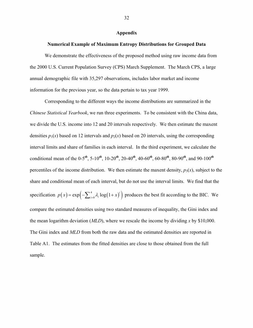
Appendix

uped Data

ncome data from

he March CPS, a large

annual demographic file with 35,297 observations, includes labor market and income

information for the previous year, so the data pertain to tax year 1999.

arized in the

ith the China data,

imate the maxent

densities p1(x) based on 12 intervals and p2(x) based on 20 intervals, using the corresponding

interval limits and share of families in each interval. In the third experiment, we calculate the

conditional mean of the 0-5th, 5-10th, 10-20th, 20-40th, 40-60th, 60-80th, 80-90th, and 90-100th

percentiles of the income distribution. We then estimate the maxent density, p3(x), subject to the

share and conditional mean of each interval, but do not use the interval limits. We find that the

Numerical Example of Maximum Entropy Distributions for Gro

We demonstrate the effectiveness of the proposed method using raw i

the 2000 U.S. Current Population Survey (CPS) March Supplement. T

Corresponding to the different ways the income distributions are summ

Chinese Statistical Yearbook, we run three experiments. To be consistent w

we divide the U.S. income into 12 and 20 intervals respectively. We then est

specification ( ) ( )( )4exp log 1 ii0i

p x xλ= − +∑ produces the best fit accord=

ing to the BIC. We

compare the estimated densities using two standard measures of inequality, the Gini index and

the mean logarithm deviation (MLD), where we rescale the income by dividing x by $10,000.

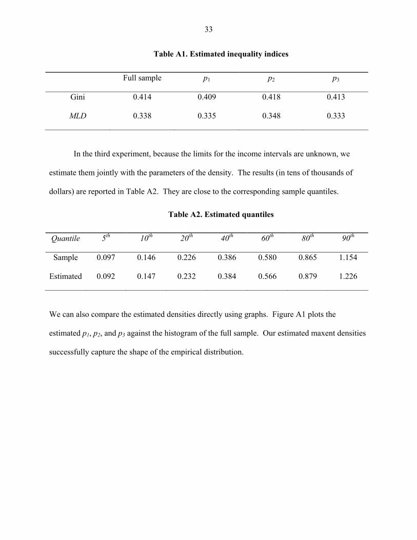
The Gini index and MLD from both the raw data and the estimated densities are reported in

Table A1. The estimates from the fitted densities are close to those obtained from the full

sample.

33

Table A1. Estimated inequality indices

ll sample p1 p p3 Fu 2

Gini 0.414 0.409 0.418 0.413

MLD 0.338 0.335 0.348 0.333

In the third experiment, because the limits for the income intervals are unknown, we

estimate them jointly with the parameters of the density. The results (in tens of thousands of

dollars) are reported in Table A2. They are close to the corresponding sample quantiles.

Table A2. Estimated quantiles

Quantile 5th 10 20 40 60th 80th 90th th th th

Sample 0.097 0.146 0.226 0.386 0.580 0.865 1.154

Estimated 0.092 0.147 0.232 0.384 0.566 0.879 1.226

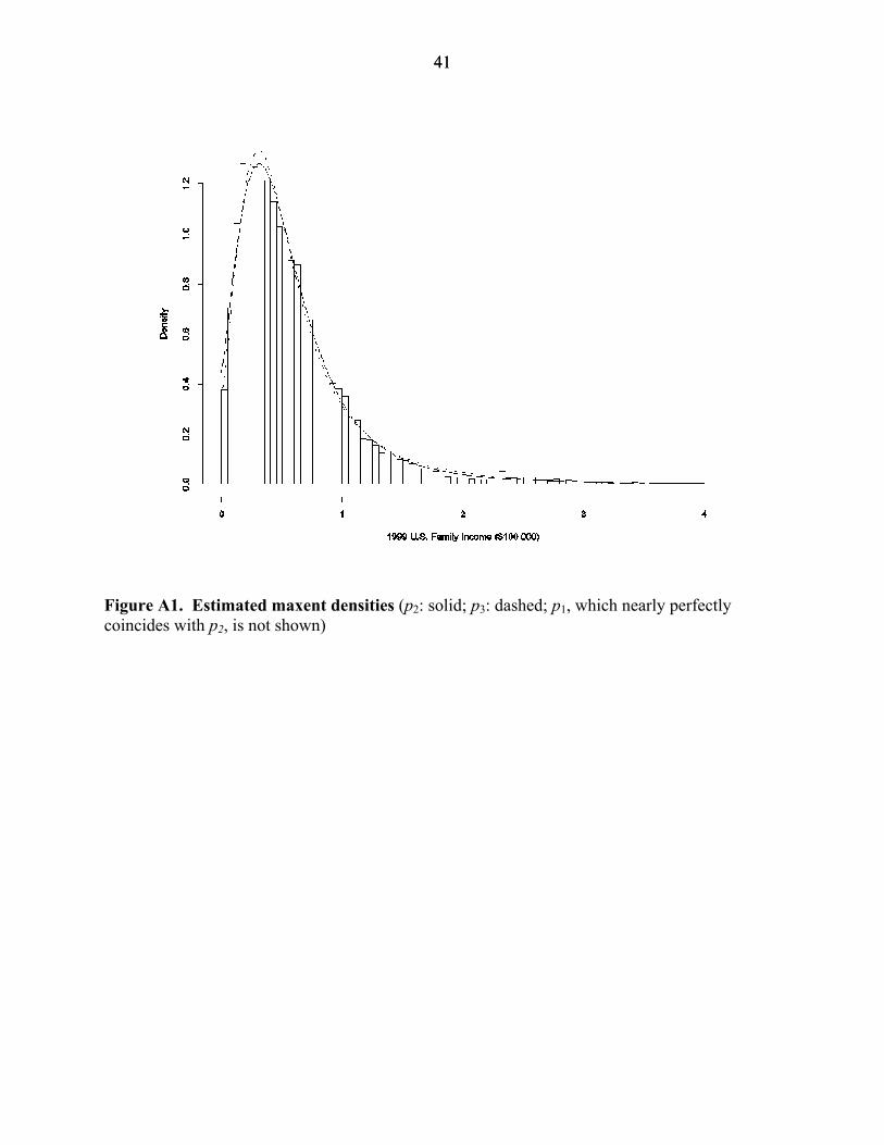
We can also compare the estimated densities directly using graphs. Figure A1 plots the

estimated p1, p2, and p3 against the histogram of the full sample. Our estimated maxent densities

successfully capture the shape of the empirical distribution.

34

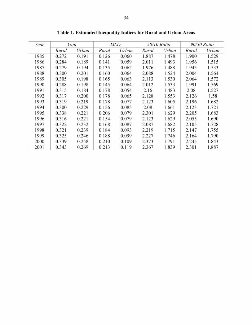
Table 1. Estimated Inequality Indices for Rural and Urban Areas

ar LD 0/1 o 90/50 Ratio

Ye Gini M 5 0 Rati ura Ur R al rba Rural Urban R l ban ural Urban Rur U n

1985 .27 0.1 0 87 47 1.900 1.529 0 2 91 .126 0.060 1.8 1. 8 1986 .28 0.1 0 11 49 1.956 1.515 0 4 89 .141 0.059 2.0 1. 3 1987 .27 0.1 0 76 48 1.945 1.533 0 9 94 .135 0.062 1.9 1. 8 1988 .30 0.2 0 88 52 2.004 1.564 0 0 01 .160 0.064 2.0 1. 4 1989 .30 0.1 0 13 530 2.064 1.572 0 5 98 .165 0.063 2.1 1. 1990 .28 0.1 0 12 53 1.991 1.569 0 8 98 .145 0.064 2.0 1. 3 1991 .31 0.1 0 4 6 48 2.08 1.527 0 5 84 .178 0.05 2.1 1. 3 1992 .31 0.2 0 28 55 2.126 1.58 0 7 00 .178 0.065 2.1 1. 3 1993 .31 0.2 0 23 60 2.196 1.682 0 9 19 .178 0.077 2.1 1. 5 1994 .30 0.2 0 8 66 2.123 1.721 0 0 29 .156 0.085 2.0 1. 1 1995 .33 0.2 0 01 62 2.205 1.683 0 8 21 .206 0.079 2.3 1. 9 1996 .31 0.2 0 23 62 2.055 1.690 0 6 21 .154 0.079 2.1 1. 9 1997 .32 0.2 0 87 68 2.105 1.728 0 2 32 .168 0.087 2.0 1. 2 1998 0.321 0.239 0.184 0.093 2.219 1.715 2.147 1.755 1999 0.325 0.246 0.188 0.099 2.227 1.746 2.164 1.790 2000 0.339 0.258 0.210 0.109 2.373 1.791 2.245 1.843 2001 0.343 0.269 0.213 0.119 2.367 1.839 2.301 1.887

35

Table 2. Comparison of Gini Coefficients

Gini Rural Urban

Source Da 8 995 1988 1995 ta Set 198 1 This study SSB 0 338 0.201 0.221 0.30 0. Li (2000) SSB .301 323 0.23 0.28 0 0. Khan and Riskin (1998) CASS .338 416 0.233 0.332 0 0. Gustafsson and Li (1999) CASS 0.228 0.276 Meng (2003) CASS 0.234 0.282

36

Table 3. Total Inequality and Its Decomposition

MLD Year Gini total within between 1985 0.310 0.164 0.111 0.053 1986 0.311 0.169 0.121 0.048 1987 0.317 0.175 0.117 0.058 1988 0.337 0.201 0.135 0.066 1989 0.342 0.208 0.138 0.070 1990 0.327 0.186 0.124 0.062 1991 0.345 0.215 0.144 0.070 1992 0.361 0.231 0.147 0.084 1993 0.380 0.255 0.150 0.105 1994 0.381 0.252 0.136 0.116 1995 0.382 0.266 0.169 0.096 1996 0.349 0.215 0.131 0.084 1997 0.375 0.258 0.143 0.116 1998 0.378 0.257 0.154 0.103 1999 0.389 0.272 0.157 0.115 2000 0.407 0.305 0.174 0.131 2001 8 0.139 0.415 0.317 0.17

ab Con tion ac to ha in lity

∆MLD ∆MLDw MLD θw θ θb θsb

T le 4. tribu of e h fac r to c nge total inequa

Year ∆ b sw

China (1985—20 01) 1985-86—1990 0 0.25 0.06

95- 0 0 0.40 0.081995-96—2000-01 1.41 0.51 0.90 0.64 -0.13 0.77 0.12

0.40 0.56 0.48 -0.08 0.47 0.09

-91 0.68 0.36 0.32 .41 -0.041990-91—19 96 .80 0.32 0.48 .39 -0.06

1985-86—2000-01 0.96 U.S. (1985—2001) 1985-86—1990-91 0.24 0.27 -0.03 0.27 0.01 -0.03 -0.011990-91—1995-96 0.90 0.89 0.01 0.87 0.02 0.02 -0.011995-96—2000-01 -0.23 -0.23 0.01 -0.24 0.01 0.01 0.011985-86—2000-01 0.30 0.31 -0.01 0.30 0.01 -0.01 -0.01

Note: All numbers have been multiplied by 100.

37

0.8 1.0

01

23

45

income

dens

ity

0.0 0.2 0.4 0.6

Figure 1. 1999 U.S. income distribution and 2001 China income distribution (U.S.: solid; China: dashes)

Note: The domains of both distributions have been re-scaled to lie within [0, 1]

0 20 40 60 80 100

0.03

0.04

0.05

0.06

0.07

0.08

0.09

income distribuiton percentile

grow

th ra

te (%

)

Figure 2. Growth incidence curve, 2001 vs. 1985

(rural: solid; urban: dashes)

38

Figure 3. Rural income distributions, 1985-2001

Figure 4: Urban income distributions, 1985-2001

39

Figure 5. Estimated rural and urban distributions in 1,000 1985 Yuan

(1985: solid: 2001: dashes and dots)

Figure 6. Rural, Urban, and Aggregate distributions for 1985 and 2001

(in 1,000 current Yuan) (rural: dots; urban: dashes and dots; aggregate: solid)

40

Figure 7. Gini index and growth rate for urban areas, 1985-2001

(income: solid; consumption dashes)

41 41

Figure A1. Estimated maxent densities (p2: solid; p3: dashed; p1, which nearly perfectly coincides with p2, is not shown)