Embed Size (px)
Citation preview
China’s Demography and its Implications
Il Houng Lee, Xu Qingjun, and Murtaza Syed
WP/13/82
© 2013 International Monetary Fund WP/13/82
IMF Working Paper
Asia and Pacific Department
China’s Demography and its Implications
Prepared by Il Houng Lee, Xu Qingjun, and Murtaza Syed1
Authorized for distribution by Il Houng Lee
March 2013
This Working Paper should not be reported as representing the views of the IMF.
The views expressed in this Working Paper are those of the author(s) and do not necessarily
represent those of the IMF or IMF policy. Working Papers describe research in progress by
the author(s) and are published to elicit comments and to further debate.
Abstract
In coming decades, China will undergo a notable demographic transformation, with its old-age
dependency ratio doubling to 24 percent by 2030 and rising even more precipitously thereafter. This
paper uses the permanent income hypothesis to reassess national savings behavior, with greater
prominence and more careful consideration given to the role played by changing demography. We
use a forward-looking and dynamic approach that considers the entire population distribution. We
find that this not only holds up well empirically but may also be superior to the static dependency
ratios typically employed in the literature. Going further, we simulate global savings behavior based
on our framework and find that China’s demographics should have induced a negative current
account in the 2000s and a positive one in the 2010s given the rising share of prime savers, only
turning negative around 2045. The opposite is true for the United States and Western Europe. The
observed divergence in current account outcomes from the simulated path appears to have been partly
policy induced. Over the next couple of decades, individual countries’ convergence toward the
simulated savings pattern will be influenced by their past divergences and future policy choices.
Other implications arising from China’s demography, including the growth model, the pension
system, the labor market, and the public finances are also briefly reviewed.
JEL Classification Numbers: E21, E27, F32, J11, J18
Keywords: China, Aging, Demographics, Savings, Current Account, Global Imbalances
Author’s E-Mail Addresses: [email protected]; [email protected]; [email protected]
1 Messrs. Lee and Syed are, respectively, the Senior and Deputy Resident Representative in the IMF’s China
office. Mr. Xu is Director of the World Economy Division in the Policy Research Department of the Ministry of
Commerce of China. We would like to thank the Ministry of Commerce and the People’s Bank of China for
hosting seminars, and staff from these institutions as well as academic experts for their valuable comments. This
paper has also benefitted from comments by the IMF China team.
2
Contents
I. Introduction ........................................................................................................................... 3
II. Literature Review ................................................................................................................. 4
III. How Does Demography Affect Savings and the Current Account? ................................... 6
A. Conceptual framework ..................................................................................................... 6
B. Simulation ........................................................................................................................ 8
Simulation I: Single-country example ............................................................................... 9
Simulation II . Multi-country context .............................................................................. 10
C. Empirical Tests ............................................................................................................... 14
IV. Other Implications of China’s Changing Demographics .................................................. 18
A. Growth and Convergence............................................................................................... 18
B. Policy Dilemma .............................................................................................................. 19
C. Pension System .............................................................................................................. 20
D. Labor Market.................................................................................................................. 21
E. Public Finances ............................................................................................................... 21
V. Conclusion ......................................................................................................................... 22
References ............................................................................................................................... 24
3
I. INTRODUCTION
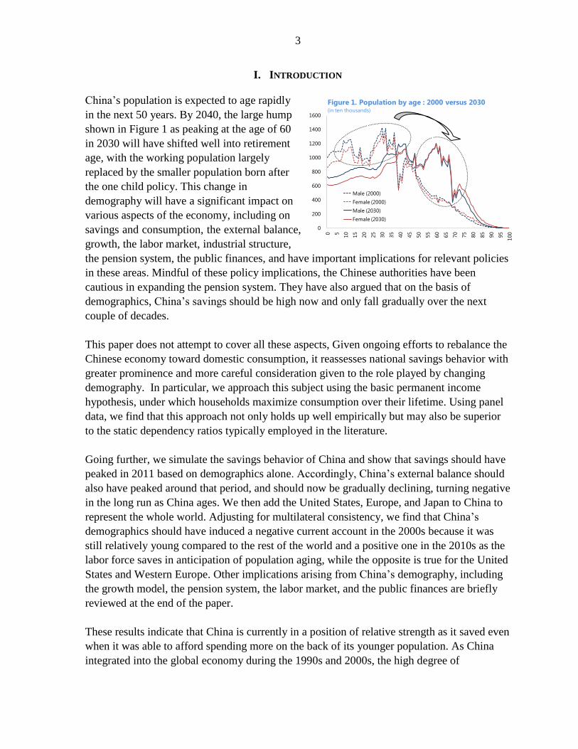
China’s population is expected to age rapidly
in the next 50 years. By 2040, the large hump
shown in Figure 1 as peaking at the age of 60
in 2030 will have shifted well into retirement
age, with the working population largely
replaced by the smaller population born after
the one child policy. This change in
demography will have a significant impact on
various aspects of the economy, including on
savings and consumption, the external balance,
growth, the labor market, industrial structure,
the pension system, the public finances, and have important implications for relevant policies
in these areas. Mindful of these policy implications, the Chinese authorities have been
cautious in expanding the pension system. They have also argued that on the basis of
demographics, China’s savings should be high now and only fall gradually over the next
couple of decades.
This paper does not attempt to cover all these aspects, Given ongoing efforts to rebalance the
Chinese economy toward domestic consumption, it reassesses national savings behavior with
greater prominence and more careful consideration given to the role played by changing
demography. In particular, we approach this subject using the basic permanent income
hypothesis, under which households maximize consumption over their lifetime. Using panel
data, we find that this approach not only holds up well empirically but may also be superior
to the static dependency ratios typically employed in the literature.
Going further, we simulate the savings behavior of China and show that savings should have
peaked in 2011 based on demographics alone. Accordingly, China’s external balance should
also have peaked around that period, and should now be gradually declining, turning negative
in the long run as China ages. We then add the United States, Europe, and Japan to China to
represent the whole world. Adjusting for multilateral consistency, we find that China’s
demographics should have induced a negative current account in the 2000s because it was
still relatively young compared to the rest of the world and a positive one in the 2010s as the
labor force saves in anticipation of population aging, while the opposite is true for the United
States and Western Europe. Other implications arising from China’s demography, including
the growth model, the pension system, the labor market, and the public finances are briefly
reviewed at the end of the paper.
These results indicate that China is currently in a position of relative strength as it saved even
when it was able to afford spending more on the back of its younger population. As China
integrated into the global economy during the 1990s and 2000s, the high degree of
0
200
400
600
800
1000
1200
1400
1600
0 5
10
15
20
25
30
35
40
45
50
55
60
65
70
75
80
85
90
95
100
Figure 1. Population by age : 2000 versus 2030 (in ten thousands)
Male (2000)
Female (2000)
Male (2030)
Female (2030)
4
underemployment and large size of new entrants to the labor market since then have
suppressed wage growth. This contributed to the decline in the wage share of GDP during
this period, allowing a large part of corporate income to be saved and reinvested. The United
States, on the other hand, will be swimming against powerful demographic currents in
attempting to achieve fiscal consolidation and reverse its trade deficit during the next decade.
During this period, demography will be pushing it toward lower savings and a current
account deficit.
We posit that the observed divergence in current account outcomes from the simulated path
may also have been the result of policy distortions. This includes expansionary
macroeconomic policies that allowed the United States to consume more than would have
been consistent with its demographic profile. Under this hypothesis, developments in across
countries were closely intertwined, mainly through the trade channel, but also through the
finance channel, as expansionary monetary policy in the United States was further fueled by
reflow of capital from China and other emerging markets through reserve accumulation of
the latter (Choi and Lee, 2010). On the Chinese side, an underdeveloped social safety net
may also have contributed to the excessive build-up of savings.
Domestically, China’s aging implies that savings will continue to remain strong over the
medium term. The size of the working population will stay relatively stable for another
decade, after which it will start to decline gradually. The expected increase in the number of
retirees over the long term poses a challenge regarding how best to manage savings to ensure
the real purchasing power per yuan saved now is not eroded over time. Savings can be
allocated between domestic investment and investment abroad, returns on which will be
determined by the efficiency of investment and the optimal portfolio management of foreign
assets, respectively. The former issue is addressed in a separate paper (Lee et al. (2013b)
forthcoming).
Over the next couple of decades, individual countries’ convergence towards the simulated
savings pattern will be influenced by their past divergences and future policy choices. The
cumulative divergence of the actual from the simulated path, be it due to labor dividend in
China or expansionary policies in the United States, will influence future household savings
behavior. If the divergence was positive, i.e., actual savings exceeded the simulated path,
then the future savings will tend to underperform the simulated path to compensate. This
assumes, of course, that policy choices are such that they help the household sector to make
optimal decisions in maximizing their consumption.
II. LITERATURE REVIEW
In recent years, there have been a number of studies on the relationship between
5
demographics and savings behavior in China.2 Using a lifecycle model, Modigliani and Cao
(2004), Horioka and Wan (2007), Horioka (2010), Song and Yang (2010), and Fan and Zhu
(2012) find evidence of a significant relationship between saving rates and the age structure
of the population.
Projecting forward, Kuijs (2006) expects China’s savings to remain high until around 2020-
25, as the negative impact on saving from a rising old-age dependency ratio is offset by the
impact of a continued decline in the young age dependency ratio. After 2025 or so, when the
former continues to increase but the latter stabilizes, the net negative effect on saving
behavior eventually becomes very substantial. Chamon and Prasad (2005) have a broadly
similar conclusion, with demographic factors by themselves implying higher household
saving over the next decade. They also suggest that these effects could switch and become
less ambiguous after around 2025, as the old-age population continues to rise and the
working-age population becomes more dominated by low-saving younger cohorts. Similarly,
Horioka and Terada-Hagiwara (2012) project China’s savings rate to continue increasing
until 2030, as its population ages relatively more slowly than a number of other Asian
economies, with its population share of retirees crossing 14 percent (the accepted definition
of an ―aged society‖) only toward the end of this period.
A few studies have also explored the potential impact of China’s demographic changes on
net savings, i.e. its current account balance. IMF (2008) uses a multi-country panel
regression to estimate determinants of current account balances, with a focus on the impact
from aging. The novel feature of the exercise is that the standard demographic variables are
expressed relative to trading partners, reflecting the fact that countries
need to be at different stages of the demographic transition in order for it to have an impact
on their external positions. With China expected to age relatively slowly compared to most of
its trading partners, the paper predicts that the impact of demographics on China’s current
account impact will remain persistently positive over the long-term, as its share of prime
savers rises relative to those of its trading partners. By contrast, the impact is significantly
negative for both the United States and Japan over the next 20-30 years and becomes
negative for Germany after around 2025.
Based on projected changes in the fraction of the population in the prime savers cohort (40-
59) around the world, Haldane (2010) and Bank of England (2011) find that medium-term
pressures on global imbalances could triple over the next twenty years, with saving rates
rising among surplus countries as their prime savers share rises (including in China) and
falling in deficit countries as their prime savers share declines (including in the United States
and other developed economies). For China, the saving rate would only start falling in the
2 A number of recent studies have also found a significant impact of demographics on savings in an
international context, including Chen et al. (2006), Fehr et al. (2007), and Krueger and Ludwig (2007).
6
late 2020s and would continue to rise as a percent of total G-20 savings at least until then. Its
current account could reach as high as 2 percent of global GDP over this period, only turning
into a deficit after 2045. While acknowledging that such a focus on demographics alone
obscures the impact on the current account of other changes like adjustments in real
exchange rates, reduced investment as the marginal product of capital falls, and lower saving
rates in emerging markets as the social safety net is further developed, the paper cautions that
these would have to be very significant to counterbalance the medium-term upward pressures
on global imbalances arising from powerful demographic forces. The results presented in our
paper are quite close in substance to the findings in these three studies.
As is typical in the literature, the empirical work in the papers discussed above relies on
reduced form regressions and static dependency ratios. By contrast, the approach in our paper
is closest in spirit to Curtis et al. (2011) in terms of taking into account the entire age
distribution and incorporating the future time-path of demographics and other variables.
Their paper finds that incorporating changing demographics in this way can help explain
much of the evolution in China’s household saving rate between 1955 and 2009. In particular,
China’s current high savings is argued to have primarily been driven by reduced family size
from the one-child policy and the relatively large share of the working-age population.
III. HOW DOES DEMOGRAPHY AFFECT SAVINGS AND THE CURRENT ACCOUNT?
A. Conceptual framework
Our framework rests on the ―permanent income‖ hypothesis. As a result, household savings
will be determined by both the demographic structure and the time horizon over which
households maximize their consumption. In this simple framework, ―household‖ represents
both consumers and producers with no public sector. An extension to include the government
can be made, but this will not have any meaningful implication on saving behavior of the
economy if both households and the government are assumed to maximize consumption over
the long run, and thus behave in the same way.
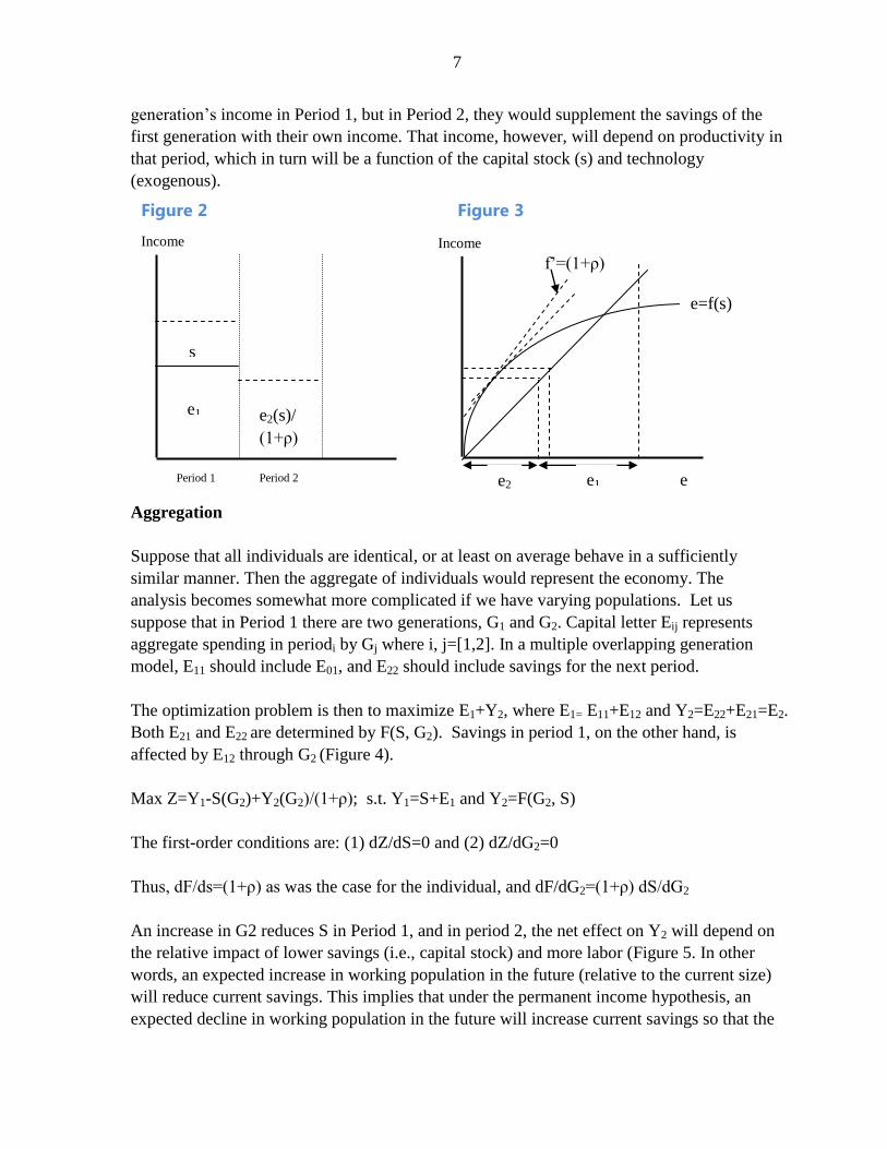
A person will maximize his/her consumption over their life span which can be divided into
period 1 and 2 (Figure 2). During period 1, the individual generates income, part of which
he/she saves so that they can live off the saving in period 2, i.e., after retirement. Thus, a
person’s maximization problem can be described as: Max e=e1+[e2/(1+ρ)] w.r.t. saving, s,
and subject to y=e1+s, and where e2= f(s) with f’>0, f‖<0, and y is predetermined by the
capital stock/productivity and technology as captured in production function f in pre-period 1.
In addition, e is consumption, y income, and ρ the discount factor for time preference.
The optimal solution represented by the first-order condition is the usual f’=(1+ρ), which can
be graphically expressed as shown above (Figure 3).
This can be extended to a multi-period model where e2(s) becomes y in the second
generation’s period 1. The second generation would then have to be financed by the first
7
generation’s income in Period 1, but in Period 2, they would supplement the savings of the
first generation with their own income. That income, however, will depend on productivity in
that period, which in turn will be a function of the capital stock (s) and technology
(exogenous).
Aggregation
Suppose that all individuals are identical, or at least on average behave in a sufficiently
similar manner. Then the aggregate of individuals would represent the economy. The
analysis becomes somewhat more complicated if we have varying populations. Let us
suppose that in Period 1 there are two generations, G1 and G2. Capital letter Eij represents
aggregate spending in periodi by Gj where i, j=[1,2]. In a multiple overlapping generation
model, E11 should include E01, and E22 should include savings for the next period.
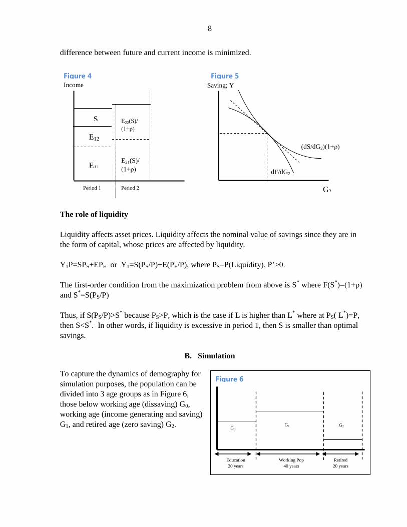
The optimization problem is then to maximize E1+Y2, where E1= E11+E12 and Y2=E22+E21=E2.
Both E21 and E22 are determined by F(S, G2). Savings in period 1, on the other hand, is
affected by E12 through G2 (Figure 4).
Max Z=Y1-S(G2)+Y2(G2)/(1+ρ); s.t. Y1=S+E1 and Y2=F(G2, S)
The first-order conditions are: (1) dZ/dS=0 and (2) dZ/dG2=0
Thus, dF/ds=(1+ρ) as was the case for the individual, and dF/dG2=(1+ρ) dS/dG2
An increase in G2 reduces S in Period 1, and in period 2, the net effect on Y2 will depend on
the relative impact of lower savings (i.e., capital stock) and more labor (Figure 5. In other
words, an expected increase in working population in the future (relative to the current size)
will reduce current savings. This implies that under the permanent income hypothesis, an
expected decline in working population in the future will increase current savings so that the
e
e2(s)/
(1+ρ)
Period 1 Period 2
e1
s
Income
f’=(1+ρ)
Income
e1 e2
e=f(s)
Figure 2 Figure 3
8
difference between future and current income is minimized.
The role of liquidity
Liquidity affects asset prices. Liquidity affects the nominal value of savings since they are in
the form of capital, whose prices are affected by liquidity.
Y1P=SPS+EPE or Y1=S(PS/P)+E(PE/P), where PS=P(Liquidity), P’>0.
The first-order condition from the maximization problem from above is S* where F(S
*)=(1+ρ)
and S*=S(PS/P)
Thus, if S(PS/P)>S* because PS>P, which is the case if L is higher than L
* where at PS( L
*)=P,
then S<S*. In other words, if liquidity is excessive in period 1, then S is smaller than optimal
savings.
B. Simulation
To capture the dynamics of demography for
simulation purposes, the population can be
divided into 3 age groups as in Figure 6,
those below working age (dissaving) G0,
working age (income generating and saving)
G1, and retired age (zero saving) G2.
E21(S)/
(1+ρ)
Income Saving; Y
G2
(dS/dG2)(1+ρ)
dF/dG2
Period 1 Period 2
E12
E11
S E22(S)/
(1+ρ)
Figure 4 Figure 5
Education
20 years
Retired
20 years
Working Pop
40 years
G0 G1 G2
Figure 6
9
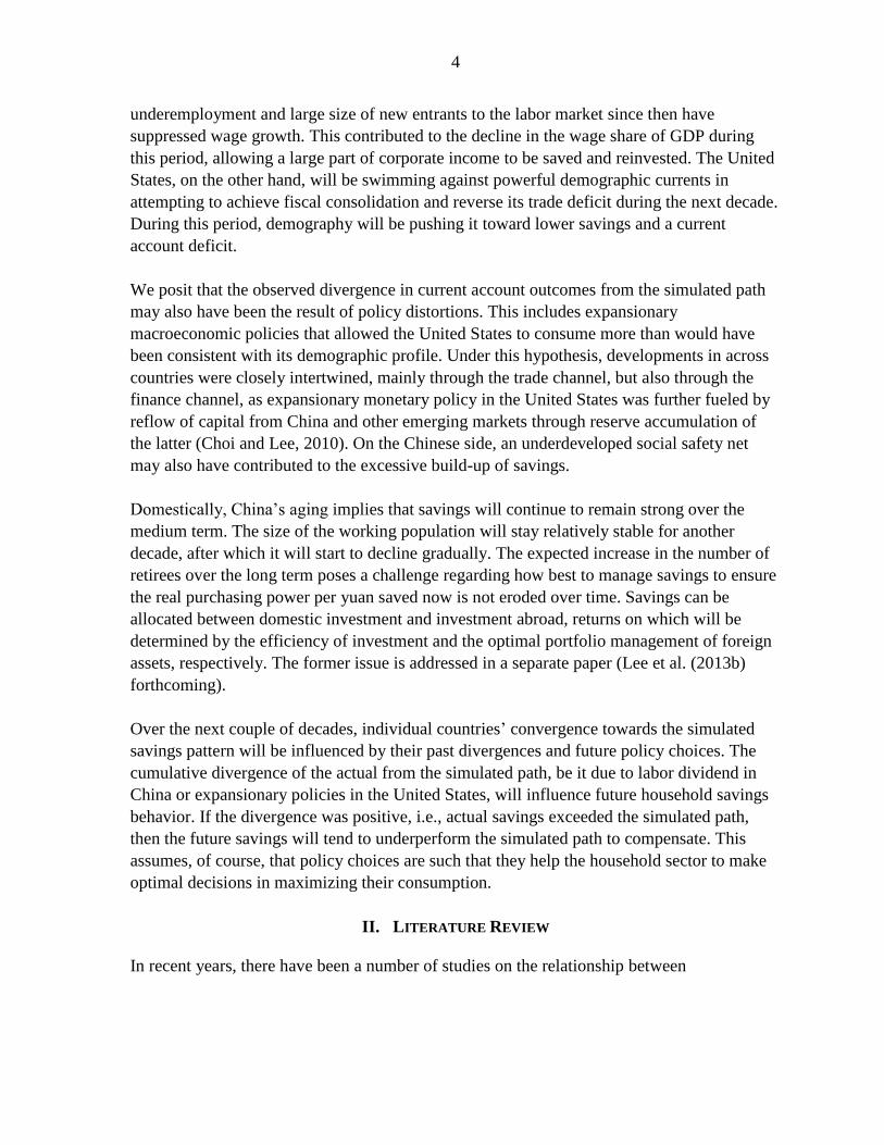
Simulation I: Single-country example
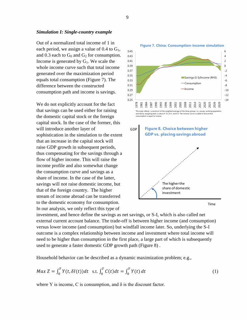
Out of a normalized total income of 1 in
each period, we assign a value of 0.4 to G1,
and 0.3 each to G0 and G2 for consumption.
Income is generated by G1. We scale the
whole income curve such that total income
generated over the maximization period
equals total consumption (Figure 7). The
difference between the constructed
consumption path and income is savings.
We do not explicitly account for the fact
that savings can be used either for raising
the domestic capital stock or the foreign
capital stock. In the case of the former, this
will introduce another layer of
sophistication in the simulation to the extent
that an increase in the capital stock will
raise GDP growth in subsequent periods,
thus compensating for the savings through a
flow of higher income. This will raise the
income profile and also somewhat change
the consumption curve and savings as a
share of income. In the case of the latter,
savings will not raise domestic income, but
that of the foreign country. The higher
stream of income abroad can be transferred
to the domestic economy for consumption.
In our analysis, we only reflect this type of
investment, and hence define the savings as net savings, or S-I, which is also called net
external current account balance. The trade-off is between higher income (and consumption)
versus lower income (and consumption) but windfall income later. So, underlying the S-I
outcome is a complex relationship between income and investment where total income will
need to be higher than consumption in the first place, a large part of which is subsequently
used to generate a faster domestic GDP growth path (Figure 8) .
Household behavior can be described as a dynamic maximization problem; e.g.,
s.t.
(1)
where Y is income, C is consumption, and δ is the discount factor.
GDP
Time
The higher the share of domestic investment
Figure 8. Choice between higher
GDP vs. placing savings abroad
-14
-12
-10
-8
-6
-4
-2
0
2
4
6
0.25
0.27
0.29
0.31
0.33
0.35
0.37
0.39
0.41
0.43
0.45
1978
1981
1984
1987
1990
1993
1996
1999
2002
2005
2008
2011
2014
2017
2020
2023
2026
2029
This scale reflects a construct of the weighted average of the three groups, i.e., young, working population,
and old by assigning each a value of 0.3, 0.4 , and 0.3. The income curve is scaled to ensure that
consumption is equal to income.
Figure 7. China: Consumption-income simulation
Savings (S-I)/Income (RHS)
Consumption
Income
10
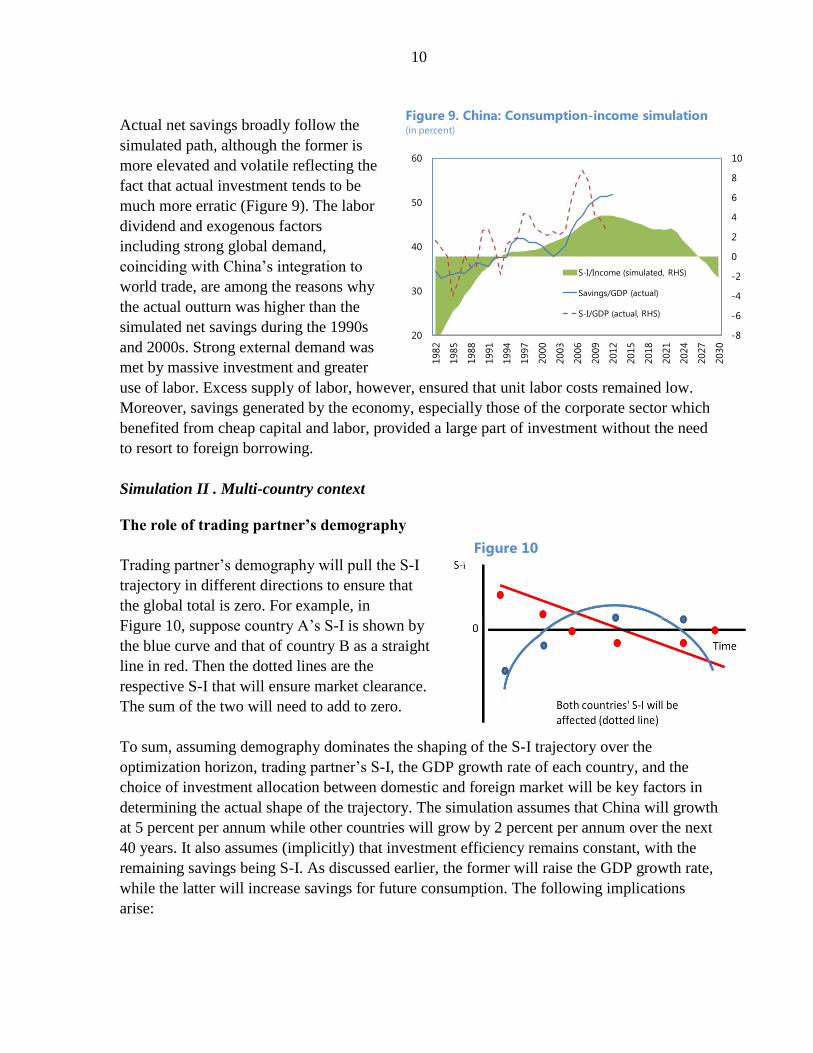
Actual net savings broadly follow the
simulated path, although the former is
more elevated and volatile reflecting the
fact that actual investment tends to be
much more erratic (Figure 9). The labor
dividend and exogenous factors
including strong global demand,
coinciding with China’s integration to
world trade, are among the reasons why
the actual outturn was higher than the
simulated net savings during the 1990s
and 2000s. Strong external demand was
met by massive investment and greater
use of labor. Excess supply of labor, however, ensured that unit labor costs remained low.
Moreover, savings generated by the economy, especially those of the corporate sector which
benefited from cheap capital and labor, provided a large part of investment without the need
to resort to foreign borrowing.
Simulation II . Multi-country context
The role of trading partner’s demography
Trading partner’s demography will pull the S-I
trajectory in different directions to ensure that
the global total is zero. For example, in
Figure 10, suppose country A’s S-I is shown by
the blue curve and that of country B as a straight
line in red. Then the dotted lines are the
respective S-I that will ensure market clearance.
The sum of the two will need to add to zero.
To sum, assuming demography dominates the shaping of the S-I trajectory over the
optimization horizon, trading partner’s S-I, the GDP growth rate of each country, and the
choice of investment allocation between domestic and foreign market will be key factors in
determining the actual shape of the trajectory. The simulation assumes that China will growth
at 5 percent per annum while other countries will grow by 2 percent per annum over the next
40 years. It also assumes (implicitly) that investment efficiency remains constant, with the
remaining savings being S-I. As discussed earlier, the former will raise the GDP growth rate,
while the latter will increase savings for future consumption. The following implications
arise:
Figure 10
-8
-6
-4
-2
0
2
4
6
8
10
20
30
40
50
60
1982
1985
1988
1991
1994
1997
2000
2003
2006
2009
2012
2015
2018
2021
2024
2027
2030
S-I/Income (simulated, RHS)
Savings/GDP (actual)
S-I/GDP (actual, RHS)
Figure 9. China: Consumption-income simulation (in percent)
11
Changes in the factors noted above could push S-I off the baseline path in the short
run, but these deviations will have to be balanced out in later years as ultimately net
savings will need to be equal to zero over the given time horizon and across countries
at each point in time.
If, for whatever reason S-I deviates from the baseline for a prolonged period, then
there will have to be an abrupt adjustment in consumption. This of course assumes
that the key fundamental affecting the baseline is demography.
If the return on S-I (investment abroad) or return on domestic investment falls, then
S-I tends to rise as people will want to ensure that their consumption level is
maintained later. The allocation between domestic and foreign investment will adjust
accordingly, with greater share going to investment that generate higher rate of return.
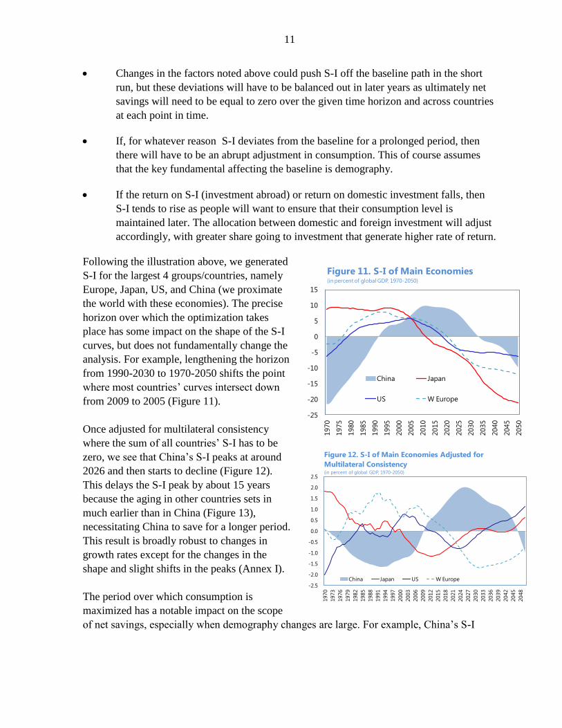
Following the illustration above, we generated
S-I for the largest 4 groups/countries, namely
Europe, Japan, US, and China (we proximate
the world with these economies). The precise
horizon over which the optimization takes
place has some impact on the shape of the S-I
curves, but does not fundamentally change the
analysis. For example, lengthening the horizon
from 1990-2030 to 1970-2050 shifts the point
where most countries’ curves intersect down
from 2009 to 2005 (Figure 11).
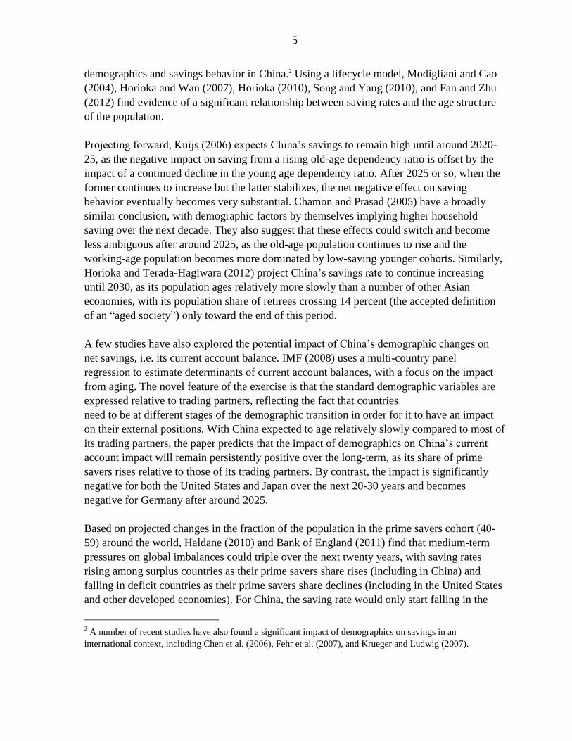
Once adjusted for multilateral consistency
where the sum of all countries’ S-I has to be
zero, we see that China’s S-I peaks at around
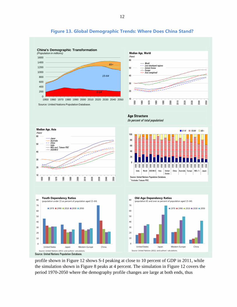
2026 and then starts to decline (Figure 12).
This delays the S-I peak by about 15 years
because the aging in other countries sets in
much earlier than in China (Figure 13),
necessitating China to save for a longer period.
This result is broadly robust to changes in
growth rates except for the changes in the
shape and slight shifts in the peaks (Annex I).
The period over which consumption is
maximized has a notable impact on the scope
of net savings, especially when demography changes are large. For example, China’s S-I
-2.5
-2.0
-1.5
-1.0
-0.5
0.0
0.5
1.0
1.5
2.0
2.5
1970
1973
1976
1979
1982
1985
1988
1991
1994
1997
2000
2003
2006
2009
2012
2015
2018
2021
2024
2027
2030
2033
2036
2039
2042
2045
2048
Figure 12. S-I of Main Economies Adjusted for
Multilateral Consistency(in percent of global GDP, 1970-2050)
China Japan US W Europe
-25
-20
-15
-10
-5
0
5
10
15
1970
1975
1980
1985
1990
1995
2000
2005
2010
2015
2020
2025
2030
2035
2040
2045
2050
Figure 11. S-I of Main Economies (in percent of global GDP, 1970-2050)
China Japan
US W Europe
12
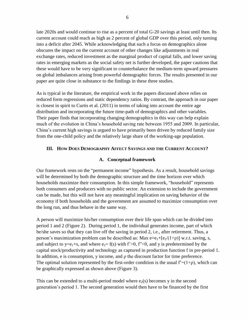
Figure 13. Global Demographic Trends: Where Does China Stand?
profile shown in Figure 12 shows S-I peaking at close to 10 percent of GDP in 2011, while
the simulation shown in Figure 8 peaks at 4 percent. The simulation in Figure 12 covers the
period 1970-2050 where the demography profile changes are large at both ends, thus
Age Structure
(In percent of total population)
Source: United Nations Population Database.
0-14
15-64
65+
0
200
400
600
800
1000
1200
1400
1600
1950 1960 1970 1980 1990 2000 2010 2020 2030 2040 2050
Source: United Nations Population Database.
China's Demographic Transformation (Population in millions)
10
20
30
40
50
60
19
50
19
60
19
70
19
80
19
90
20
00
20
10
20
20
20
30
20
40
20
50
WorldLess-developed regionsUnited StatesEuropeAsia (weighted)
Median Age, World (Years)
10
20
30
40
50
60
19
50
19
60
19
70
19
80
19
90
20
00
20
10
20
20
20
30
20
40
20
50
JapanAustraliaChinaIndiaNIEs excl. Taiwan POCASEAN-5
Median Age, Asia(Years)
0
20
40
60
80
1002
00
5
20
50
20
05
20
50
20
05
20
50
20
05
20
50
20
05
20
50
20
05
20
50
20
05
20
50
20
05
20
50
20
05
20
50
20
05
20
50
India World ASEAN-5 Asia United
States
China Australia Europe NIEs 1/ Japan
0-14 15-64 65+
Source: United Nations Population Database.
1 Excludes Taiwan POC.
0
10
20
30
40
50
60
70
80
United States Japan Western Europe China
1970 1990 2010 2030 2050
Youth Dependency Ratios(population under 15 as percent of population aged 15-64)
Source: United Nations (2011) and authors' calculations.
0
10
20
30
40
50
60
70
80
United States Japan Western Europe China
1970 1990 2010 2030 2050
Old-Age Dependency Ratios(population 65 and over as percent of population aged 15-64)
Source: United Nations (2011) and authors' calculations.
13
necessitating much larger savings during 2010-2030 period. The simulation in Figure 8
maximizes consumption only over the 1980-2030 period, which does not capture the large
drops at both ends. Most likely, the shorter time horizon is closer to reality as demographic
projections could change depending on changes in the birth rate, mortality rate, and
participation rate.
In addition to fundamentals in classical growth models including the capital stock, labor, and
productivity changes, other macroeconomic policy changes could also induce a change in the
shape and timing of the curvatures. However, these deviations will have to be compensated
later on because demographic forces are ultimately overpowering and cannot be resisted
indefinitely. For example, an overly generous pension scheme will push up consumption
beyond that consistent with the permanent income hypothesis. However, later, consumption
has to be restricted in order to finance the over consumption in earlier years.
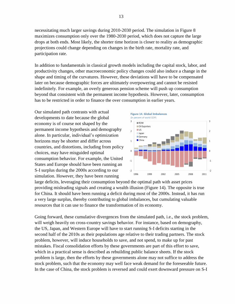
Our simulated path contrasts with actual
developments to date because the global
economy is of course not shaped by the
permanent income hypothesis and demography
alone. In particular, individual’s optimization
horizons may be shorter and differ across
countries, and distortions, including from policy
choices, may have misguided optimal
consumption behavior. For example, the United
States and Europe should have been running an
S-I surplus during the 2000s according to our
simulation. However, they have been running
large deficits, leveraging their consumption beyond the optimal path with asset prices
providing misleading signals and creating a wealth illusion (Figure 14). The opposite is true
for China. It should have been running a deficit during most of the 2000s. Instead, it has run
a very large surplus, thereby contributing to global imbalances, but cumulating valuable
resources that it can use to finance the transformation of its economy.
Going forward, these cumulative divergences from the simulated path, i.e., the stock problem,
will weigh heavily on cross-country savings behavior. For instance, based on demography,
the US, Japan, and Western Europe will have to start running S-I deficits starting in the
second half of the 2010s as their populations age relative to their trading partners. The stock
problem, however, will induce households to save, and not spend, to make up for past
mistakes. Fiscal consolidation efforts by these governments are part of this effort to save,
which in a practical sense is described as rebuilding public balance sheets. If the stock
problem is large, then the efforts by these governments alone may not suffice to address the
stock problem, such that the economy may well face weak demand for the foreseeable future.
In the case of China, the stock problem is reversed and could exert downward pressure on S-I
-2
-1
0
1
2
3
-2
-1
0
1
2
3
1996 1999 2002 2005 2008 2011
ROW
Oil Exporters
US
Japan
Germany
China
Global Imbalances(In percent of world GDP)
Figure 14. Global Imbalances
(In percent of world GDP)
14
beyond what demography itself might dictate. In particular, the younger generation, which
has shown a much higher propensity for consumption, is expected to add to the downward
pressure.
C. Empirical Tests
In this section, we test whether the underlying assumptions for the simulation above, i.e., the
permanent income hypothesis and the role of demography, really matter.
Permanent income hypothesis and demography
As before, we define G0, G1, and G2 to represent the young, working-age and retired
population, respectively
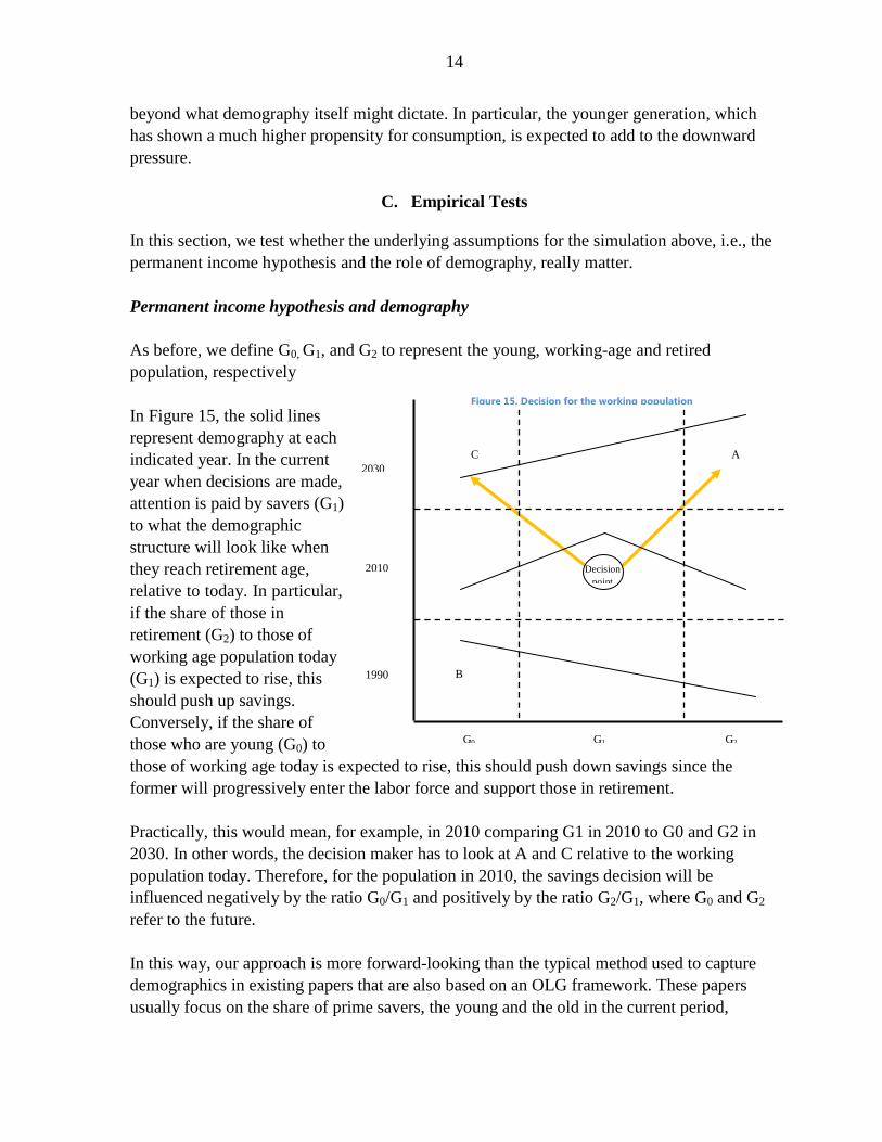
In Figure 15, the solid lines
represent demography at each
indicated year. In the current
year when decisions are made,
attention is paid by savers (G1)
to what the demographic
structure will look like when
they reach retirement age,
relative to today. In particular,
if the share of those in
retirement (G2) to those of
working age population today
(G1) is expected to rise, this
should push up savings.
Conversely, if the share of
those who are young (G0) to
those of working age today is expected to rise, this should push down savings since the
former will progressively enter the labor force and support those in retirement.
Practically, this would mean, for example, in 2010 comparing G1 in 2010 to G0 and G2 in
2030. In other words, the decision maker has to look at A and C relative to the working
population today. Therefore, for the population in 2010, the savings decision will be
influenced negatively by the ratio G0/G1 and positively by the ratio G2/G1, where G0 and G2
refer to the future.
In this way, our approach is more forward-looking than the typical method used to capture
demographics in existing papers that are also based on an OLG framework. These papers
usually focus on the share of prime savers, the young and the old in the current period,
Decision
point
A
B
C
Figure 15. Decision for the working population
in 2010
2030
2010
1990
2030
G0 G1 G2
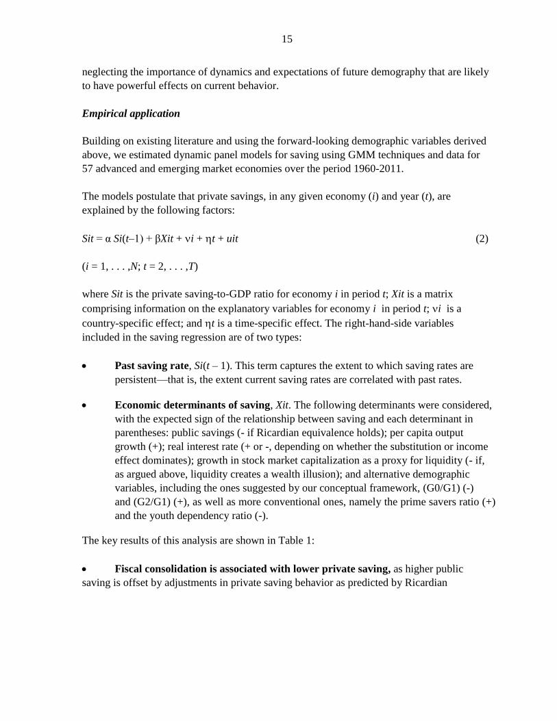
15
neglecting the importance of dynamics and expectations of future demography that are likely
to have powerful effects on current behavior.
Empirical application
Building on existing literature and using the forward-looking demographic variables derived
above, we estimated dynamic panel models for saving using GMM techniques and data for
57 advanced and emerging market economies over the period 1960-2011.
The models postulate that private savings, in any given economy (i) and year (t), are
explained by the following factors:
Sit = α Si(t–1) + βXit + i + t + uit (2)
(i = 1, . . . ,N; t = 2, . . . ,T)
where Sit is the private saving-to-GDP ratio for economy i in period t; Xit is a matrix
comprising information on the explanatory variables for economy i in period t; i is a
country-specific effect; and t is a time-specific effect. The right-hand-side variables
included in the saving regression are of two types:
Past saving rate, Si(t – 1). This term captures the extent to which saving rates are
persistent—that is, the extent current saving rates are correlated with past rates.
Economic determinants of saving, Xit. The following determinants were considered,
with the expected sign of the relationship between saving and each determinant in
parentheses: public savings (- if Ricardian equivalence holds); per capita output
growth (+); real interest rate (+ or -, depending on whether the substitution or income
effect dominates); growth in stock market capitalization as a proxy for liquidity (- if,
as argued above, liquidity creates a wealth illusion); and alternative demographic
variables, including the ones suggested by our conceptual framework, (G0/G1) (-)
and (G2/G1) (+), as well as more conventional ones, namely the prime savers ratio (+)
and the youth dependency ratio (-).
The key results of this analysis are shown in Table 1:
Fiscal consolidation is associated with lower private saving, as higher public
saving is offset by adjustments in private saving behavior as predicted by Ricardian
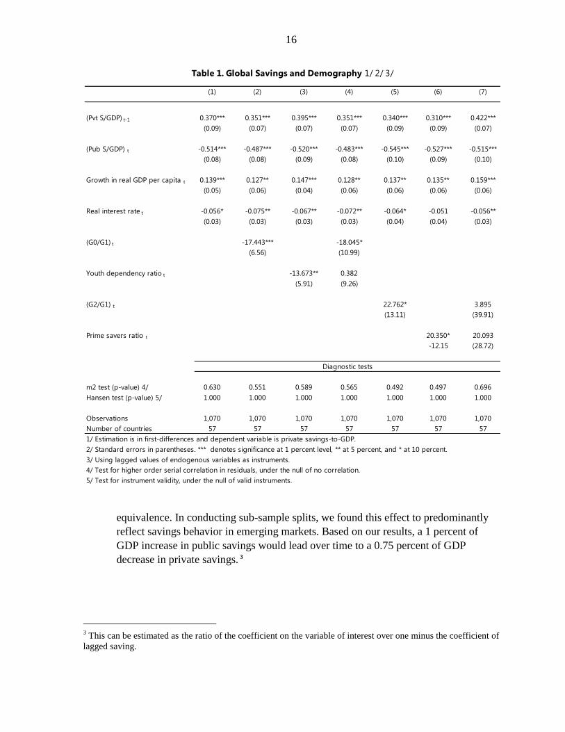
16
equivalence. In conducting sub-sample splits, we found this effect to predominantly
reflect savings behavior in emerging markets. Based on our results, a 1 percent of
GDP increase in public savings would lead over time to a 0.75 percent of GDP
decrease in private savings. 3
3 This can be estimated as the ratio of the coefficient on the variable of interest over one minus the coefficient of
lagged saving.
(1) (2) (3) (4) (5) (6) (7)
(Pvt S/GDP) t-1 0.370*** 0.351*** 0.395*** 0.351*** 0.340*** 0.310*** 0.422***
(0.09) (0.07) (0.07) (0.07) (0.09) (0.09) (0.07)
(Pub S/GDP) t -0.514*** -0.487*** -0.520*** -0.483*** -0.545*** -0.527*** -0.515***
(0.08) (0.08) (0.09) (0.08) (0.10) (0.09) (0.10)
Growth in real GDP per capita t 0.139*** 0.127** 0.147*** 0.128** 0.137** 0.135** 0.159***
(0.05) (0.06) (0.04) (0.06) (0.06) (0.06) (0.06)
Real interest rate t -0.056* -0.075** -0.067** -0.072** -0.064* -0.051 -0.056**
(0.03) (0.03) (0.03) (0.03) (0.04) (0.04) (0.03)
(G0/G1) t -17.443*** -18.045*
(6.56) (10.99)
Youth dependency ratio t -13.673** 0.382
(5.91) (9.26)
(G2/G1) t 22.762* 3.895
(13.11) (39.91)
Prime savers ratio t 20.350* 20.093
-12.15 (28.72)
m2 test (p-value) 4/ 0.630 0.551 0.589 0.565 0.492 0.497 0.696
Hansen test (p-value) 5/ 1.000 1.000 1.000 1.000 1.000 1.000 1.000
Observations 1,070 1,070 1,070 1,070 1,070 1,070 1,070
Number of countries 57 57 57 57 57 57 57
1/ Estimation is in first-differences and dependent variable is private savings-to-GDP.
4/ Test for higher order serial correlation in residuals, under the null of no correlation.
5/ Test for instrument validity, under the null of valid instruments.
Table 1. Global Savings and Demography 1/ 2/ 3/
Diagnostic tests
2/ Standard errors in parentheses. *** denotes significance at 1 percent level, ** at 5 percent, and * at 10 percent.
3/ Using lagged values of endogenous variables as instruments.
17
Higher output growth boosts saving. A sustained 1 percentage point increase in per
capita output growth over time leads to an almost 0.2 percent of GDP increase in the
private saving rate.
An increase in the rate of return decreases savings. While saving and real interest
rates are generally expected to be positively related—with the strength of this
relationship likely to depend on the size of households’ net asset position (Deaton
(1992)—we uncovered a negative impact. This is consistent with the recent literature
on target savings, under which the income effect of interest rate changes dominates
savings behavior. We also found this effect to be predominantly a feature of the
emerging markets in our sample.
Both the forward-looking demographic variables developed in the earlier section
are significant determinants of private savings and enter with the expected sign
(Table1, columns 2 and 5). As the ratio of young people in the future is expected to
rise, private savings decline. The opposite effect is detected if the ratio of the elderly
is projected to rise in coming decades. The effects are also economically significant,
with a 1 percentage point increase in G0/G1 (G2/G1) over time reducing (increasing)
private savings by 0.25 percentage points of GDP.
Moreover, there is also some evidence that these dynamic demographic variables
are superior to the static ones typically employed in the literature. While the
youth-dependency ratio (column 3) and prime saver share (column 6) are significant
and enter our regressions with the expected sign, as found in other studies, the former
is knocked out by our forward-looking G0/G1 variable (column 4), suggesting that
the demographic information it captures is superior for explaining private savings.
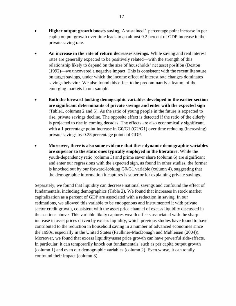
Separately, we found that liquidity can decrease national savings and confound the effect of
fundamentals, including demographics (Table 2). We found that increases in stock market
capitalization as a percent of GDP are associated with a reduction in saving. In our
estimations, we allowed this variable to be endogenous and instrumented it with private
sector credit growth, consistent with the asset price channel of excess liquidity discussed in
the sections above. This variable likely captures wealth effects associated with the sharp
increase in asset prices driven by excess liquidity, which previous studies have found to have
contributed to the reduction in household saving in a number of advanced economies since
the 1990s, especially in the United States (Faulkner-MacDonagh and Mühleisen (2004)).
Moreover, we found that excess liquidity/asset price growth can have powerful side-effects.
In particular, it can temporarily knock out fundamentals, such as per capita output growth
(column 1) and even our demographic variables (column 2). Even worse, it can totally
confound their impact (column 3).
18
IV. OTHER IMPLICATIONS OF CHINA’S CHANGING DEMOGRAPHICS
A. Growth and Convergence
A quick review of countries that managed to narrow the gap between their own and the US
GDP per capita indicates that political stability and sound governance structures are
prerequisite and necessary conditions for convergence. However, they are not sufficient and
it seems that additional impetus is required to maintain sustained growth, namely rapid
expansion of global trade, matched by large domestic investments. This is what China has
(1) (2) (3)
(Pvt S/GDP) t-1 0.282*** 0.241*** 0.251***
(0.08) (0.09) (0.08)
(Pub S/GDP) t -0.591*** -0.621*** -0.640***
(0.09) (0.11) (0.12)
Growth in real GDP per capita t 0.097 0.120* 0.121*
(0.08) (0.07) (0.07)
Real interest rate t -0.104*** -0.093*** -0.097***
(0.03) (0.03) (0.03)
Growth in stock market cap t -0.015* -0.016* -0.017*
(0.01) (0.01) (0.01)
(G0/G1) t -12.039 23.612
(11.63) (22.47)
(G2/G1) t -13.673**
(5.91)
m2 test (p-value) 4/ 0.630 0.551 0.589
Hansen test (p-value) 5/ 1.000 1.000 1.000
Observations 758 758 758
Number of countries 54 54 54
1/ Estimation is in first-differences and dependent variable is private savings-to-GDP.
4/ Test for higher order serial correlation in residuals, under the null of no correlation.
5/ Test for instrument validity, under the null of valid instruments.
Table 2. Exploring the Role of Liquidity 1/ 2/ 3/
Diagnostic tests
2/ Standard errors in parentheses. *** , ** and * denote significance at 1, 5, and 10 percent level, respectively.
3/ Using lagged values of endogenous variables as instruments. Stockmarket cap instrumented by credit growth.
19
been doing also. Strong external demand that followed the WTO accession was matched by a
rapid supply response, made possible by massive investment and abundant supply of labor.
Expected changes in China’s demography will limit labor supply and thereby start raising
unit labor costs. With population aging, investment will also likely fall as the returns to
capital fall relative to scarcer labor and declining savings make capital more expensive.
Thus, demographic changes will add to the challenge of defining a new growth model as
trade expansion and investment, the traditional engines of growth, will likely no longer be
available to the same extent. In that sense, it seems international experience is only of
relatively limited use in terms of defining the main engines that can help China sustain its
growth. Instead, it appears that China will have to rely on home-grown solutions in terms of
the precise engines that will help it achieve convergence with advanced economies.
Of course, the shrinking labor force may be partly offset if changes are introduced in
government policies such as the one-child-policy or if there is an increase in immigration or
participation rates, although these would take time to take effect. Moreover, total factor
productivity gains from innovation, education, and labor mobility (partly through
urbanization) could also raise per capita income and thereby affect savings.
B. Policy Dilemma
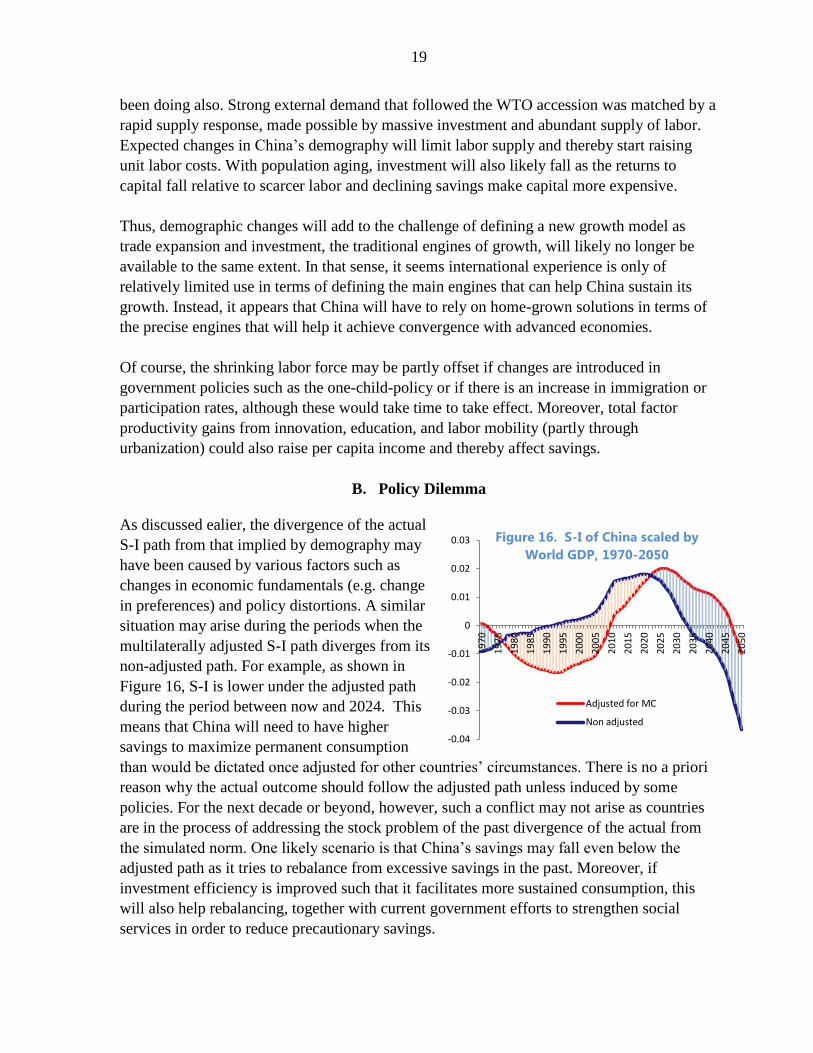
As discussed ealier, the divergence of the actual
S-I path from that implied by demography may
have been caused by various factors such as
changes in economic fundamentals (e.g. change
in preferences) and policy distortions. A similar
situation may arise during the periods when the
multilaterally adjusted S-I path diverges from its
non-adjusted path. For example, as shown in
Figure 16, S-I is lower under the adjusted path
during the period between now and 2024. This
means that China will need to have higher
savings to maximize permanent consumption
than would be dictated once adjusted for other countries’ circumstances. There is no a priori
reason why the actual outcome should follow the adjusted path unless induced by some
policies. For the next decade or beyond, however, such a conflict may not arise as countries
are in the process of addressing the stock problem of the past divergence of the actual from
the simulated norm. One likely scenario is that China’s savings may fall even below the
adjusted path as it tries to rebalance from excessive savings in the past. Moreover, if
investment efficiency is improved such that it facilitates more sustained consumption, this
will also help rebalancing, together with current government efforts to strengthen social
services in order to reduce precautionary savings.
-0.04
-0.03
-0.02
-0.01
0
0.01
0.02
0.03
19
70
19
75
19
80
19
85
19
90
19
95
20
00
20
05
20
10
20
15
20
20
20
25
20
30
20
35
20
40
20
45
20
50
Figure 16. S-I of China scaled by
World GDP, 1970-2050
Adjusted for MC
Non adjusted
20
C. Pension System
While only the urban pension system is
examined here, the implications from the
illustration below will also apply to other part
of China’s multi-layered pension system. There
are currently 285 million participants in the
urban employees’ basic pension insurance
system, of which 215 million are contributors
and 70 million recipients or retirees. The total
size of the pension fund as of end 2011 stood at
RMB 2 trillion. The benefit per retiree in 2011
at RMB 18,700 is about three times the
contribution per employee. However, with the
size of contributors about 3 times the retirees and fiscal contributions making up around a
fifth of total payment, the pension fund has been growing steadily from about 1 percent of
GDP in 2001 to 4.2 percent of GDP in 2011. The rate of return, however, has been relatively
weak at 3.5 percent per year (average during the last 10 years) which is broadly the deposit
rate.
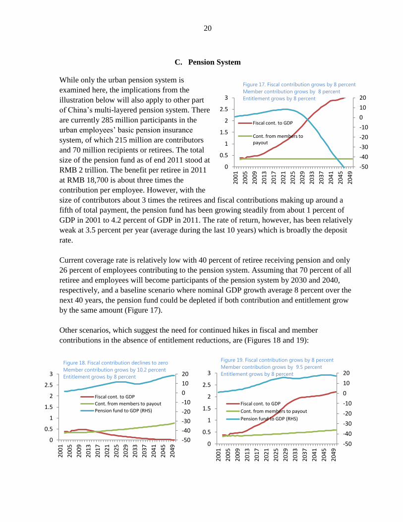
Current coverage rate is relatively low with 40 percent of retiree receiving pension and only
26 percent of employees contributing to the pension system. Assuming that 70 percent of all
retiree and employees will become participants of the pension system by 2030 and 2040,
respectively, and a baseline scenario where nominal GDP growth average 8 percent over the
next 40 years, the pension fund could be depleted if both contribution and entitlement grow
by the same amount (Figure 17).
Other scenarios, which suggest the need for continued hikes in fiscal and member
contributions in the absence of entitlement reductions, are (Figures 18 and 19):
-50
-40
-30
-20
-10
0
10
20
0
0.5
1
1.5
2
2.5
3
20
01
20
05
20
09
20
13
20
17
20
21
20
25
20
29
20
33
20
37
20
41
20
45
20
49
Figure 18. Fiscal contribution declines to zero
Member contribution grows by 10.2 percent
Entitlement grows by 8 percent
Fiscal cont. to GDP
Cont. from members to payout
Pension fund to GDP (RHS)
-50
-40
-30
-20
-10
0
10
20
0
0.5
1
1.5
2
2.5
3
20
01
20
05
20
09
20
13
20
17
20
21
20
25
20
29
20
33
20
37
20
41
20
45
20
49
Figure 19. Fiscal contribution grows by 8 percent
Member contribution grows by 9.5 percent
Entitlement grows by 8 percent
Fiscal cont. to GDP
Cont. from members to payout
Pension fund to GDP (RHS)
-50
-40
-30
-20
-10
0
10
20
0
0.5
1
1.5
2
2.5
3
20
01
20
05
20
09
20
13
20
17
20
21
20
25
20
29
20
33
20
37
20
41
20
45
20
49
Figure 17. Fiscal contribution grows by 8 percent
Member contribution grows by 8 percent
Entitlement grows by 8 percent
Fiscal cont. to GDP
Cont. from members to payout
21
D. Labor Market
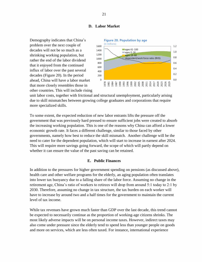
Demography indicates that China’s
problem over the next couple of
decades will not be so much as a
shrinking working population, but
rather the end of the labor dividend
that it enjoyed from the continued
influx of labor over the past several
decades (Figure 20). In the period
ahead, China will have a labor market
that more closely resembles those in
other countries. This will include rising
unit labor costs, together with frictional and structural unemployment, particularly arising
due to skill mismatches between growing college graduates and corporations that require
more specialized skills.
To some extent, the expected reduction of new labor entrants lifts the pressure off the
government that was previously hard pressed to ensure sufficient jobs were created to absorb
the increasing working population. This is one of the reasons why China can afford a lower
economic growth rate. It faces a different challenge, similar to those faced by other
governments, namely how best to reduce the skill mismatch. Another challenge will be the
need to cater for the dependent population, which will start to increase in earnest after 2024.
This will require more savings going forward, the scope of which will partly depend on
whether it can ensure the value of the past saving can be retained.
E. Public Finances
In addition to the pressures for higher government spending on pensions (as discussed above),
health care and other welfare programs for the elderly, an aging population often translates
into lower tax buoyancy due to a falling share of the labor force. Assuming no change in the
retirement age, China’s ratio of workers to retirees will drop from around 5:1 today to 2:1 by
2030. Therefore, assuming no change in tax structure, the tax burden on each worker will
have to increase by around two and a half times for the government to maintain the current
level of tax income.
While tax revenues have grown much faster than GDP over the last decade, this trend cannot
be expected to necessarily continue as the proportion of working-age citizens shrinks. The
most likely adverse impacts will be on personal income taxes. However, indirect taxes may
also come under pressure since the elderly tend to spend less than younger people on goods
and more on services, which are less often taxed. For instance, international experience
0.0
0.2
0.4
0.6
0.8
1.0
1.2
0
200
400
600
800
1000
1200
1400
1600
1978
1981
1984
1987
1990
1993
1996
1999
2002
2005
2008
2011
2014
2017
2020
2023
2026
2029
Figure 20. Population by age(in millions)
ages 61-100
ages 0-18
ages 19-60
dependent/work force ratio (RHS)
22
cautions that the drop in tax receipts associated with aging is especially pronounced for
income and payroll taxes, but also affects sales and property taxes.
To meet enhanced funding requirements for old-age expenditures, governments have
typically had to modernize their tax systems. This involves efforts to keep existing tax bases
from being eroded, as well as extending them into new areas, including reducing tax
preferences, increasing dividends from state-owned enterprises, enhancing natural resource
and energy taxation, increasing taxes on services, and diversifying and making revenue
sources more broad-based (such as reducing reliance on taxes that the elderly are less able to
pay out of fixed incomes).
V. CONCLUSION
Despite the divergence of actual net savings from the predicted path based on demography,
empirical tests lend support to demography being an important determinant of savings. What
are the potential policy implications of our findings?
First, demography dictates that China will experience a continued external current account
surplus for a prolonged period as its population will still age relatively slowly than most of its
main competitors over this period. With China’s aging setting in much later, its population
would likely want to save more. The stock of saving to date, however, will pull in the other
direction. The announced policies to promote consumption and income inequality are to
some extent geared toward achieving this intertemporal rebalancing. Strengthened social
services and proper compensation of factors of production (labor and capital) will raise
consumption as savings will likely fall as income share shifts from the rich to the poor and
from corporates to households. The rationale is that in the absence of income inequality and
full compensation of factors of input (which underlies the simulation results), China would
have spent more in the past decade and less in the coming decade. Going forward, therefore,
current policies will need to be geared towards correcting the past distortions that led to
higher than demography-consistent savings.
Second, there could be some tension among countries as each strives to attain the savings that
would optimize consumption over its lifetime cycle. In China, for example, its multilaterally
adjusted next savings should be lower in the next decade and higher in the following two
decades thereafter because it ages relatively slowly compared to other countries. However,
because China over-saved in previous years, the inter-temporal rebalancing needed to unwind
this should help the global outcome to align more closely with the multilaterally consistent S-
I path. Similarly, the next two decades thereafter, higher savings could be attainable by
advanced countries if they deleverage and consolidate their fiscal position sufficiently to
build up savings to make up for their previous lack of thrift. To avoid adding another
distortion, it will be important to ensure that China’s stock of savings generates adequate
23
returns. If returns are low, this will, other things being equal, add additional pressure for
savings.
Third, China’s changing demographics make it essential to find a new growth model, since it
can no longer rely on a large labor dividend and savings. A tightening labor market will start
shifting income away from corporates to households. Even without the corrective policies
discussed above, this shift will reduce corporate sector saving and investment, and raise
household income and consumption. With corrective policies, the marginal propensity of
consumption will also be larger. Thus, if investment is to be curtailed going forward as
financing conditions tighten and especially amid growing concerns about excess capacity
and continued overinvestment, then the only way to maintain robust growth is to start reaping
dividends from efficiency gains and innovation. In terms of the labor market, China will need
to make up for tightening conditions with better training for labor to reduce skill mismatches
that will otherwise become an increasing constraint under a new growth paradigm.
Fourth, China’s impending demographic changes suggest the need for caution in expanding
the pension system. Continuation of the current status quo could run down pension funds in
the next two decades as the pension scheme is expanded at a time when the number of
retirees also starts to increase. While an expansion of the pension system is called for to
ensure it covers a wider population, it will need to be carefully calibrated with inflows as an
overly generous payouts could threaten the viability of the pension system in the future.
Fifth, in addition to increased old-age related spending obligations, China’s tax revenues
could come under pressure as the share of the working population shrinks in coming decades.
This could put pressure on China’s traditionally prudent public finances, necessitating
countervailing changes in tax policy and administration that prevent the erosion of the tax
base and extend it in new areas, including resources, energy and services sectors.
24
REFERENCES
Bank of England, 2011, ―The Future of International Capital Flows‖, Financial Stability
Paper No. 12 – December 2011 (William Speller, Gregory Thwaites and Michelle
Wright).
Chamon, Marcos and Eswar Prasad, 2005, ―Determinants of Household Saving in China‖,
International Monetary Fund, mimeo.
Chen, Kaiji, Ayse •Imrohoroglu, and Selahattin • Imrohoroglu, 2007, ―The Japanese
Saving Rate Between 1960 and 2000: Productivity, Policy Changes, and
Demographics‖, Economic Theory, 32, pp. 87-104.
Fan Xuchun and Zhu Baohua, 2012, ―China' s Life Expectancy Growth,Age Structure
Change and National Saving Rate‖, Population Research, 36(4).
Curtis, C., S. Lugauer, N. Mark, 2011, ―Demographic Patterns and Household Saving in
China‖, NBER Working Paper No. 16828.
Deaton, Angus, 1992, Understanding Consumption, Clarendon Lectures on Economics
(Oxford: Oxford University Press).
Faulkner-MacDonagh, Chris, and Martin Mühleisen, 2004, ―Are U.S. Households Living
Beyond Their Means?‖ Finance and Development, Vol. 41, No. 1, pp. 36–9.
Fehr, Hans, Sabine Jokisch, and Laurence J. Kotliko, 2007, ―Will China Eat Our Lunch or
Take Us to Dinner? Simulating the Transition Paths of the United States, the
European Union, Japan, and China‖, Fiscal Policy and Management in East Asia,
NBER-EASE, Volume 16, University of Chicago Press, pp. 133-193.
Haldane, A., 2010, ―Global imbalances in retrospect and prospect‖, available at
www.bankofengland.co.uk/publications/speeches/2010/speech468.pdf .
Hoiroka, Charles Yuji and Junmin Wan, 2006, ―The Determinants of Household Saving in
China: A Dynamic Panel Analysis of Provincial Data‖, Journal of Money, Credit, and
Banking, 39(8), pp. 2077-96.
Horioka, Charles Yuji, 2010, ―Aging and Saving in Asia‖, Pacific Economic Review, 15, pp.
46-55.
25
Horioka, Charles Yuji, and Terada-Hagiwara, Akiko, 2011, ―The Determinants and Long-
term Projections of Saving Rates in Developing Asia‖, Japan and the World
Economy 24(2), pp. 128-137.
International Monetary Fund, 2005, ―Global Imbalances: A Saving and Investment
Perspective‖, World Economic Outlook (September: Washington DC).
International Monetary Fund, 2008, ―The Graying of Asia: Demographics, Capital Flows,and
Financial Markets‖, Asia and Pacific Regional Economic Outlook (November:
Washington DC).
Krueger, Dirk and Alexander Ludwig, 2007, ―On the Consequence of Demographic Change
for Rates of Returns to Capital, and the Distribution of Wealth and Welfare‖, Journal
of Monetary Economics, 54(1), pp. 49-87.
Kuijs, L., 2006, ―How will China’s saving-investment balance evolve?‖, World Bank Policy
Research Working Paper, No 3958, July.
Ma, Guonan and Wang Yi, 2010, ―China's High Saving Rate: Myth and Reality‖, BIS
Working Paper, Number 312.
Modigliani, Franco and Shi Larry Cao, 2004, ―The Chinese Saving Puzzle and the Life-Cycle
Hypothesis‖, Journal of Economic Literature, 42, pp. 145-170.
Song, Zheng Michael and Dennis Tao Yang, 2010, ―Life Cycle Earnings and Saving in a
Fast-Growing Economy‖, mimeo, Chinese University of Hong Kong.
United Nations, 2011, ―World Population Prospects: The 2010 Revision‖ (CD-ROM
Edition)—Extended Dataset in Excel and ASCII formats. New York: Population
Division, Department of Economic and Social Affairs, United Nations.
Woon Gyu Choi and Il Houng Lee, 2010, ―Monetary Transmission of Global Imbalances in
Asian Countries‖ IMF Working Paper WP/10/214 (International Monetary Fund:
Washington DC).
26
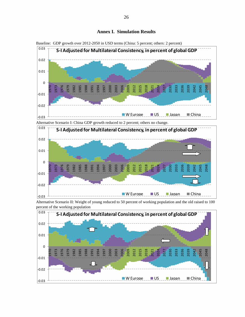
Annex I. Simulation Results
Baseline: GDP growth over 2012-2050 in USD terms (China: 5 percent; others: 2 percent)
Alternative Scenario I: China GDP growth reduced to 2 percent; others no change.
Alternative Scenario II: Weight of young reduced to 50 percent of working population and the old raised to 100
percent of the working population
-0.03
-0.02
-0.01
0
0.01
0.02
0.031
97
0
19
73
19
76
19
79
19
82
19
85
19
88
19
91
19
94
19
97
20
00
20
03
20
06
20
09
20
12
20
15
20
18
20
21
20
24
20
27
20
30
20
33
20
36
20
39
20
42
20
45
20
48
S-I Adjusted for Multilateral Consistency, in percent of global GDP
W Europe US Japan China
-0.03
-0.02
-0.01
0
0.01
0.02
0.03
19
70
19
73
19
76
19
79
19
82
19
85
19
88
19
91
19
94
19
97
20
00
20
03
20
06
20
09
20
12
20
15
20
18
20
21
20
24
20
27
20
30
20
33
20
36
20
39
20
42
20
45
20
48
S-I Adjusted for Multilateral Consistency, in percent of global GDP
W Europe US Japan China
-0.03
-0.02
-0.01
0
0.01
0.02
0.03
19
70
19
73
19
76
19
79
19
82
19
85
19
88
19
91
19
94
19
97
20
00
20
03
20
06
20
09
20
12
20
15
20
18
20
21
20
24
20
27
20
30
20
33
20
36
20
39
20
42
20
45
20
48
S-I Adjusted for Multilateral Consistency, in percent of global GDP
W Europe US Japan China