Children's cognitive ability, schooling and work: Evidence from Ethiopia

International Journal of Educational Development 38 (2014) 22–36

Children’s cognitive ability, schooling and work: Evidence fromEthiopia

Seife Dendir *

Department of Economics, Radford University, Radford, VA 24142, USA

A R T I C L E I N F O

Keywords:

Cognitive ability

Endowment

Human capital

Schooling

Child work

Ethiopia

A B S T R A C T

I investigate the relationship between children’s cognitive ability and parental investment using a rich

dataset on a cohort of children from Ethiopia. The data come from Young Lives, a long-term international

study of childhood poverty in four countries. Ability is measured by scores on a cognitive test. A child’s

enrollment in school, participation in work and work hours are employed as measures of parental

investment in human capital. The results provide strong evidence of reinforcing parental investment –

higher ability children are more likely to be enrolled in school and less likely to work and, conditional on

participation, also work fewer hours. These results are mostly robust to addressing potential feedback

effects between schooling and test scores and household heterogeneities. On the policy front, the results

suggest that the seeds of adulthood inequality in human capital and earnings capability may be sown

quite early in childhood, and thereby underscore the importance of interventions that, among others,

attempt to improve prenatal and early life health and nutrition, which are often cited as the sources of

deficiencies in children’s cognitive ability.

� 2014 Elsevier Ltd. All rights reserved.

Contents lists available at ScienceDirect

International Journal of Educational Development

jo ur n al ho m ep ag e: ww w.els evier . c om / lo cat e/ i jed u d ev

1. Introduction

The pattern of allocation of resources by parents amongoffspring with varying endowments can be compensating orreinforcing. Compensating allocations provide more resources tothe less endowed, to enable equitable opportunities and quality oflife later in adulthood. Early models of household utilitymaximization with intergenerational provision of resourcesassumed that parents inherently possess such a preference forequity among their children, and hence for compensatingallocations (Becker and Tomes, 1976). However, this assumptionwas challenged soon after, on theoretical grounds as well as withevidence that market signals, such as differential earningopportunities in adulthood, can shape and dominate householdbehavior, possibly leading to reinforcing allocations (Behrmanet al., 1982; Rosenzweig and Schultz, 1982). Very likely, idiosyn-cratic preferences combine with market mechanisms to determinethe final nature of investments, the dynamics of which are highlydependent on relevant household characteristics, society’s generallevel of development, market imperfections, and the degree ofsocial and economic inequality. Such nonlinearities render the

* Tel.: +1 540 831 5437; fax: +1 540 831 6209.

E-mail address: [email protected]

http://dx.doi.org/10.1016/j.ijedudev.2014.06.007

0738-0593/� 2014 Elsevier Ltd. All rights reserved.

nature of intra-household allocation of resources largely empiricaland contextual (Behrman, 1997).

Human capital investment often constitutes a core componentof resources allocated to children by parents (the other takes theform of ‘transfers’). Given preferences, testable implicationsconsistent with compensating, reinforcing or neutral investmentsin human capital are derived from consensus models of the family(Behrman et al., 1982; Behrman, 1997 provides an extended review).Empirical tests, in turn, have mostly investigated differences ininvestment by a child’s sex. This is mainly due to the fact that sexis the most directly observable genetic endowment.1 Variations inchildren’s health endowment and whether parents invest tocompensate or reinforce such inequalities have also been empha-sized (see Pitt et al., 1990 for a seminal contribution).

A child’s cognitive or educational ability, despite the presumedcentral role it plays in the efficiency (returns and costs) of humancapital investment broadly, and educational investments specifi-cally, has been the subject of fewer studies. This is largely because[innate] cognitive ability is unobservable to the researcher.Although they are available, IQ or ability tests are usually difficult

1 Also, gender exhibits interesting interactions with parental preferences,

production technology and culture which, in combination, often translate into

differences in general labor market opportunities, giving it a special role in studies

that examine the endowment–investment relationship (Rosenzweig and Schultz,

1982; Behrman and Deolalikar, 1995).

http://crossmark.crossref.org/dialog/?doi=10.1016/j.ijedudev.2014.06.007&domain=pdf

http://crossmark.crossref.org/dialog/?doi=10.1016/j.ijedudev.2014.06.007&domain=pdf


mailto:[email protected]

http://www.sciencedirect.com/science/journal/07380593

www.elsevier.com/locate/ijedudev


S. Dendir / International Journal of Educational Development 38 (2014) 22–36 23

to administer alongside large-scale household surveys that alsocollect the requisite information on a wide array of controlvariables. In spite of this difficulty from the point of view of theresearcher, it can be argued that parents can adequately assesstheir children’s ability, in relative if not absolute terms, and willlikely condition their investment allocations on such differences inperceived ability.

In theory at least, the prevalent pattern of educationalinvestment allocation is expected to be of the reinforcing type.To the extent that marginal product of investment in humancapital increases in child endowment, an ‘‘economic’’ allocationshould favor more endowed children. There are factors that couldattenuate and may even alter this, however, including inequality-averse parental preferences. Specific parametric assumptionsabout the human capital production and parental welfarefunctions are also crucial, as are total resources available forparents for allocation (Behrman, 1997).

In this study I examine the nature of the association betweenchildren’s educational endowment and parental investment inschooling using a unique longitudinal survey from Ethiopia. Thecontributions to the literature derive from the following. First, ituses a direct measure of children’s perceived endowment. In tworounds of the survey, the full sample of children completed awidely known standardized test of cognitive ability. Controlling fora rich array of child and household characteristics, the studytherefore tests whether poor Ethiopian households conditioneducational investment decisions on their assessment of a child’sability and, if so, whether these decisions follow reinforcement orcompensation. Only a handful of recent studies have used directmeasures of ability in this context. Second, the educationalinvestment decision is examined from two angles – child schoolingand work. This is relevant because studies have shown that thesetwo are not necessarily substitutes and drawing inferences aboutone (e.g. schooling status) based on the other (e.g. child work) cansometimes be fallacious.2 More importantly, by examining childwork as a separate parental decision variable, the study alsocontributes to the now-extensive child labor literature that hasalmost entirely been unable to evaluate or isolate the endowmenteffect on child work in poor developing economies. In doing so, theeffect on both the extensive and intensive margins of child labor isanalyzed.

Bacolod and Ranjan (2008) is the study closest to this one inadopting a direct measure of educational endowment to examinethe impact on child schooling as well as work. Using data from theCebu metropolitan area in the Philippines, they report thatchildren with higher scores on an IQ test are more likely to bein school even in poor (low wealth) households. Conversely,households of even moderate wealth may be opting to let low-ability children stay idle rather than sending them to school orwork. The study, however, does not consider the amount orintensity of child work. Two more studies, Ayalew (2005) andAkresh et al. (2012a), employ data from a village in Ethiopia and aprovince in Burkina Faso, respectively, to measure children’sability using test scores and examine the association with childschooling. Both report higher rates of school enrollment for higherability children. Neither study considered child work.3

2 Among other reasons, this could be due to the potential confounding effects of

leisure (Ravallion and Wodon, 2000) and idleness (Biggeri et al., 2003), or possible

complementarity between schooling and work (Admassie, 2003). Kim (2009)

argues the suggested complementarity between schooling and work that is

highlighted in some policy circles is often not grounded in evidence.3 To the best of my knowledge, Ayalew (2005) is the first study to adopt a direct

measure of endowment (i.e. score on an ability test) in the specific literature.

Interestingly, he also reports that although households seem to reinforce

educational endowment, investment in health is compensating – less endowed

children receive more health-related resources.

Third, the data employed have attributes that are especiallypertinent to a study of this type: (a) the cohort children aresurveyed at two important junctures – ages 12 and 15 – whenparents’ say is still arguably the most important factor determininga child’s status (e.g. in schooling and work), hence the latter’s use toproxy parental human capital investment decisions; (b) the samplehas extremely low attrition, which minimizes selection bias oftenassociated with cohort data; (c) unlike most of the above-citedstudies that were confined to a particular area/region, the samplein this study comes from about 20 sites in five major regions ofEthiopia, providing a balanced representation of the country’sgeographical, cultural and regional diversity, and enabling poten-tially broader inferences from the results; and (d) the surveys tookplace during a period in which Ethiopia recorded arguably thefastest growth in its economy as well as the largest expansion inschooling opportunities for children, especially at the primary level.The repeated cross-sectional analysis therefore is able to capture theimpact, if any, the changing socio-economic conditions have had onthe endowment–child schooling/work relationship.

Finally, it should be noted that estimation of the endowmenteffect using cognitive test score suffers from potential bias mainlybecause whether such a score measures pure ability is debatable.For instance, it is possible that test score at least partially reflectscurrent and past schooling inputs and achievement, inducingreverse causation. More generally, unobserved household char-acteristics can also cause bias in cross-sectional estimations. Thepaper attempts to address these problems by using, respectively, a‘residual method’ that utilizes the longitudinal nature of the dataand estimation of a within-household model on sibling pairs.

The paper is organized as follows. The next section givesbackground of the study context by highlighting relevant statisticsand determinants of child schooling and work in Ethiopia. Section3 describes the data, variables of interest and some bivariateassociations. Section 4 provides the empirical framework, followedby baseline results and sensitivity analyses in Section 5. Section 6discusses the results in the context of existing findings. The lastsection concludes and offers some policy remarks. The resultsgenerally point to a pattern of reinforcing investment by Ethiopianhouseholds in children’s education: (a) Higher ability, as measuredby score on an ability test, is positively correlated with a child’senrollment in school; (b) The likelihood of participating in marketwork is negatively associated with perceived ability; (c) Condi-tional on participation, higher ability children work fewer hours;and (d) Although these associations are between concurrent testscore and child status at each age, they are also present afteraccounting for potential sources of bias. For example, they alsohold firm when ability is measured as a residual to account forpotential reciprocal effect from schooling, and when an alternatespecification is used to account for unobserved householdcharacteristics.

2. Study context

Historically, Ethiopia had a poor record in various measures ofchildren’s schooling. At the turn of the Millennium, gross primaryenrollment was about 62% and entry rate to primary school at thenormal age (7 years) was 20%, both of which were significantlyworse than the corresponding averages for Sub-Saharan Africa(SSA) (World Bank, 2005). Reform efforts that began in 1993 hadgathered pace in the last decade, however, allowing the country toregister impressive results on certain fronts. A central objective ofthe government’s educational reform program was increasingaccess to schooling, particularly in rural areas and at the primarylevel. That objective is largely being achieved. As of 2011, forexample, net primary enrollment reached 86%, compared to a SSAaverage of 75% (World Bank, 2013).

4 The sites were located in five regions/administrative states of the country:

Addis Ababa, Amhara, Oromia, Southern Nations, Nationalities and Peoples’ Region

(SNNP), and Tigray.

S. Dendir / International Journal of Educational Development 38 (2014) 22–3624

Other dimensions of schooling are lagging, however. Comple-tion rates are low. In 2011, primary completion rate was 58%,relative to a SSA average of 70% (World Bank, 2013). The push toexpand access may also have significantly compromised quality.Resources per student, such as teacher to student and textbook tostudent ratios, are under considerable downward pressure due tofinancing constraints. Disparities in attainment by sex and locationpersist (Woldehanna et al., 2008b; Woldehanna, 2011a; Derconand Singh, 2013; Rolleston, 2014; Frost and Little, 2014).

On the demand side, parental education, household income andwealth are shown to be important determinants of children’sschool enrollment and progress. In rural areas, for example, Maniet al. (2013) report that having a mother (father) with non-zeroschooling increases the chances of a child’s enrollment by 3–7 (7–10) percentage points. Income elasticity of primary enrollment isestimated to be 0.3–0.9, and the income effect is even stronger ongrade attainment and for girls. Sibling composition factors are alsoimportant. Generally, having more siblings and being a later-bornchild raise the chances of school enrollment (Woldehanna et al.,2008b). Although the evidence is mixed, distance to school andhousehold shocks appear to have a negative impact on enrollment(Himaz, 2013; Woldehanna et al., 2008b).

By many accounts, child labor is also widespread in Ethiopia.Analysis of the first national labor force survey indicated thataverage participation rates for 7–14 year-old boys (girls) inmarket work were 52% (42%) in rural areas and 14% (8%) inurban areas. For household work, the corresponding rates were22% (41%) and 36% (52%) in rural and urban areas, respectively(Alvi and Dendir, 2011). A national child labor force survey laterfound that 62.4% of 10–14 year-olds were economically active(CSA, 2003). These ratios place the country high in a ranking bythe incidence of child labor, even amongst SSA countries.

Furthermore, studies document that, generally, children’swork burden negatively impacts enrollment and progress inschool. Notwithstanding gender-based differences in participa-tion by type of work, on average children from less educated andcredit-constrained households are more likely to participate inwork full-time or to combine work with school (Woldehannaet al., 2008a; Alvi and Dendir, 2011; Orkin, 2012). Wealth andassets have a complex effect, however. Woldehanna et al. (2008a)estimate that below a certain threshold, rising wealth isassociated with a higher probability that a child will combineschooling with work (relative to schooling only), whereas ahousehold’s land holdings did not have a significant effect onchildren’s time use.

Some forms of social capital, for example household groupmembership, lessen the chances that a child will only involve inlabor activities. Others, such as localized cultural norms may havea facilitative effect on child work, however, by sanctioning the viewthat children’s contributions to household labor and resources arenot only beneficial but also inevitable (Orkin, 2010). Finally, achild’s age and birth order also determine the likelihood ofinvolving in work, whereby older and earlier-born children are in arelatively disadvantaged position relative to their younger, later-born siblings (Alvi and Dendir, 2011).

At the policy level, some have argued that the country’s coredevelopment strategy – known as Agricultural Development LedIndustrialization (ADLI), which aims to raise rural labor forceparticipation, incomes and agricultural credit, especially forwomen – perhaps had unintended negative consequences forchildren’s status. Woldehanna et al. (2008a) argue, for instance,that promotion of labor-intensive agricultural production mayhave led to higher demand for child labor on rural farms,consequently harming schooling. In another evidence, Orkin(2010) notes that the government’s Productive Safety Net Program(PSNP), introduced in 2005 to combat food insecurity by offering

families daily wages for unskilled work, has in some instancesincreased child labor supply. Although the PSNP does not formallyavail the services of children, it is not uncommon for children tosubstitute for, or work alongside, their parents or other registeredhousehold members. Finally, the rise in women’s labor supplywithout concurrent improvements in social and physical infra-structure for child care may have shifted household workresponsibilities to female children (Woldehanna et al., 2008a).

3. Descriptive analysis

3.1. Data

Data for the study come from the Young Lives (YL) project, a 15-year longitudinal study of childhood poverty at the Department ofInternational Development, University of Oxford. The projectinvolves 12,000 children in four countries: Ethiopia, India (AndhraPradesh), Peru and Vietnam. Starting in 2002, the project hasfollowed two cohorts of children in each country: the ‘YoungerCohort’ of 2000 children aged around 1 in 2002 and the ‘OlderCohort’ of 1000 children aged around 8 in 2002. In addition to thefirst round, so far the project has collected two more rounds of dataon these children, in 2006 (aged 5 and 12) and 2009 (aged 8 and15). The project has the stated aims of understanding the causesand consequences of childhood poverty and thereby informing thedevelopment of policies that will reduce it. To fulfill theseobjectives, the YL study collects extensive information on wide-ranging economic, social and environmental phenomena at thechild, household and community levels.

I use data from the Ethiopia part of the YL project. The YLsampling procedure adopted sentinel site surveillance, where thesites were purposefully selected to meet study objectives, such asits poverty-centered focus, to optimize study sustainability, and tocapture geographical and cultural diversity of the country andurban–rural differences. This was followed by random sampling ofhouseholds within each site. Accordingly, the sample provides abalanced representation of the Ethiopian geographical, culturaland regional diversity.4 Furthermore, even though the survey is notnationally representative and cannot be used for monitoring ofwelfare indicators over time (e.g. as in the Demographic and HealthSurvey (DHS) and Welfare Monitoring Survey (WMS)), it is notedthat the YL sample is an appropriate and valuable medium for themodeling, analysis and understanding of the dynamics of childwelfare in Ethiopia (Outes-Leon and Sanchez, 2008).

For this particular study the latter two rounds of data on the‘Older Cohort’ of children (henceforth also identified by age at thetime of survey: Age 12 and Age 15) are used. I focus on the oldercohort because their ages during the surveys span a critical periodin children’s school status and involvement in household andoutside work activities. Children in Ethiopia are expected to startschool at age 7 and progress through most of primary school by age14. The data at ages 12 and 15 therefore provide valuablesnapshots of a child’s schooling status and progress around themiddle and supposed late years of primary education. Further-more, these are also ages when parents will arguably assume thatchildren are physically and mentally maturing to be able tocommence and increasingly engage in household and/or outsidework. In poor households where direct and indirect/opportunitycosts of a child’s schooling are viewed as considerable, the yearscovered by the two rounds of data represent a critical period ofdecision-making in terms of allocation of resources and children’s

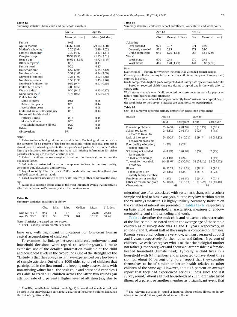
Table 1aSummary statistics: basic child and household variables.

Age 12 Age 15

Mean (std. dev.) Mean (std. dev.)

Female 0.49

Age in months 144.65 (3.81) 179.84 (3.60)

Mother’s schoolinga 2.20 (3.64) 2.19 (3.62)

Father’s schoolinga 3.30 (4.42) 3.33 (4.41)

Caregiver’s age 39.39 (9.56) 41.95 (9.51)

Head’s age 46.62 (11.35) 48.72 (11.54)

Other caregiverb 0.13 0.13

Female head 0.26 0.27

Household size 6.52 (2.05) 6.35 (2.12)

Number of adults 3.51 (1.67) 4.44 (2.09)

Number of siblings 3.25 (1.93) 3.02 (1.88)

Number of sisters 1.58 (1.30) 1.45 (1.26)

Number of children <5 0.59 (0.74) 0.47 (0.65)

Child’s birth order 4.00 (2.56)

Wealth indexc 0.30 (0.17) 0.35 (0.17)

Nondurable PCEd 4.73 (0.58) 4.82 (0.57)

Child’s healthe

Same as peers 0.61 0.48

Better than peers 0.28 0.44

Worse than peers 0.11 0.08

Child had serious illness/injury 0.16 0.14

Household health shocksf

Father’s illness 0.15 0.15

Mother’s illness 0.20 0.22

Household member’s illness 0.20 0.25

Urban 0.40 0.42

Observations 971

Notes:a Refers to that of biological mother’s and father’s. The biological mother is also

the caregiver for 88 percent of the base observations. When biological parent/s is

absent, parents’ schooling reflects the caregiver’s and partner’s (i.e. mother/father

figure’s) education. Observations that have still missing information for either

parent’s schooling are assigned a value of zero.b Refers to children whose caregiver is neither the biological mother nor the

biological father.c 0–1 index constructed based on component indices for housing quality,

consumer durables/assets, and services.d Log of monthly total real (base 2006) nondurable consumption (food plus

nonfood) expenditure per adult.e Based on child’s assessment of own health relative to other children of the same

age.f Based on a question about some of the most important events that negatively

affected the household’s economy since the previous round.

Table 1bSummary statistics: measures of ability.

Obs. Min. Max. Median Mean Std. dev.

Age 12: PPVTa 945 11 127 72 75.88 26.18

Age 15: PPVT 971 38 203 161 151.91 34.26

Notes: Statistics are based on raw scores.a PPVT, Peabody Picture Vocabulary Test.

Table 1cSummary statistics: children’s school enrollment, work status and work hours.

Age 12 Age 15

Obs. Mean (std. dev.) Obs. Mean (std. dev.)

Schooling

Ever enrolled 971 0.97 971 0.99

Currently enrolled 971 0.95 971 0.90

Grade completed 945 3.25 (1.63) 964 5.55 (2.05)

Worka

Work status 970 0.48 970 0.46

Work hours 465 3.28 (1.79) 444 3.80 (2.38)

Notes:

Ever enrolled – dummy for whether the child ever attended formal school.

Currently enrolled – dummy for whether the child is currently (as of survey date)

enrolled in school.

Grade completed – highest grade completed as of survey date by ever enrolled child.a Based on reported child’s time-use during a typical day in the week prior to

survey date.

Work status – equals one if child reported non-zero hours in work for pay or on

family farm/business, zero otherwise.

Work hours – hours of work for pay or on family farm/business on a typical day in

the week prior to the survey; statistics are conditional on participation.

Table 1dSelf- and caregiver-reported primary reasons for school non-enrollment.

Reason Age 12 Age 15

Child Caregiver Child Caregiver

Financial problems 7 (14.3%) 4 (8.2%) 10 (10.1%) 9 (9.1%)

School too far or

unsafe to travel to

2 (4.1%) 2 (4.1%) 2 (2%) 1 (1%)

Lack of interest or

behavioral problems

5 (10.2%) 5 (10.2%) 9 (9.1%) 19 (19.2%)

Poor quality education/

school facilities

1 (2%) 1 (2%)

Schooling not needed

for job/trade

4 (8.2%) 3 (6.1%) 3 (3%) 2 (2%)

To look after siblings 2 (4.1%) 1 (2%) 1 (1%)

To work for household

or for pay

14 (28.6%) 15 (30.6%) 39 (39.4%) 39 (39.4%)

Illness 6 (12.2%) 6 (12.2%) 8 (8.1%) 9 (9.1%)

To look after ill or

elderly family members

2 (4.1%) 1 (2%) 5 (5.1%) 2 (2%)

Family issues or conflict 1 (2%) 2 (4.1%) 5 (5.1%) 7 (7.1%)

Other or reason not given 5 (10.2%) 9 (18.4%) 18 (18.2%) 10 (10.1%)

Observations 49 99


time use, with significant implications for long-term humancapital accumulation of children.5

To examine the linkage between children’s endowment andhousehold decisions with regard to schooling/work, I makeextensive use of the detailed information available at the childand household levels in the two rounds. One of the strengths of theYL study is that the surveys so far have experienced very low levelsof sample attrition. Out of the 1000 older cohort of children thatparticipated in the first round and keeping only observations withnon-missing values for all the basic child and household variables, Iwas able to track 971 children across the latter two rounds (anattrition rate of 3 percent). Higher level of attrition (e.g. due to

5 As will be noted below, the first round (Age 8) data on the older cohort could not

be used in this study because only about a quarter of the sample children had taken

the test of cognitive ability.

migration) are often associated with systematic changes in a cohortsample and lead to bias in analysis, but the very low attrition rate inthe YL surveys means this is highly unlikely. Summary statistics onthe variables of interest are presented in Tables 1a–1c, respectivelyon basic child and household characteristics, measures of endow-ment/ability, and child schooling and work.

Table 1a describes the basic child and household characteristicsof the final sample. As noted earlier, the average age of the samplechildren as of survey date was 12 and 15 years, respectively, inrounds 2 and 3. About half of the sample is composed of females.Parents’ years of schooling are very low, with an average of about 2and 3 years, respectively, for the mother and father. 13 percent ofchildren live with a caregiver who is neither the biological mothernor father (Other caregiver) and about a quarter reside in a female-headed household (Female head). Typically, a child lives in ahousehold with 6.4 members and is expected to have about threesiblings. About 90 percent of children report that they considerthemselves to be of similar or better health relative to otherchildren of the same age. However, about 15 percent on averagereport that they had experienced serious illness since the lastsurvey round.6 About a fifth of households of YL children also listedillness of a parent or another member as a significant event that

6 The relevant question in round 2 inquired about serious illness or injury,

whereas in round 3 it was just about serious illness.


adversely affected their economy. On average, 41 percent of thesample children come from urban areas.

For the purposes of this paper, a child’s endowment is measuredby her score on a test of cognitive ability or intelligence. The oldercohort in the YL study completed two such tests in the three roundsof data collection: the Raven’s Colored Progressive Matrices (CPM)in round 1 (age 8) and Peabody Picture Vocabulary Test (PPVT) inrounds 2 and 3 (ages 12 and 15). Unfortunately in the Ethiopianversion, administration of the Raven’s test in the first round raninto difficulties relating to explanation of tasks and timeconstraints and thus only about a quarter of the sample – allurban children – have test scores available in the dataset. This isthe reason why the analysis in this paper makes use of only thelatter two rounds of the Ethiopian YL data. Cueto et al. (2009) notethat these problems, coupled with further difficulties encoun-tered in the Peruvian pilot tests for round 2, prompted theabandonment of the CPM, though it may yet be brought back forfuture rounds.7

The PPVT, which was adopted for rounds 2 and 3, is a test widelyapplied to measure verbal ability/scholastic aptitude and generalcognitive development since its inception in 1959. It is untimed,does not require reading on the part of the respondent, is relativelyeasy to administer, and can be completed in about 20–30 min. Thetest is documented to have strong positive correlation with othercommon measures of intelligence such as the Wechsler andMcCarthy Scales (see Campbell, 1998; Campbell et al., 2001, amongothers), although the evidence on the extent to which it is entirelyfree from cultural bias is contested. The object of the exercise to thetest-taker is to identify one picture, among a set of four picturespresented, that corresponds to a word read out by the examiner.The test has gone through many revisions over time and PPVT-III(Dunn and Dunn, 1997; Form A) was the version used in YL rounds2 and 3. The PPVT contains 17 sets of 12 items each, arranged inorder of difficulty, and the starting set for a respondent variesdepending on his/her age. Progress through (up or down) sets isdecided by performance during the test, eventually determiningwhat are known as the Basal and Ceiling Item sets for eachindividual. Scores are then computed by subtracting the number oferrors from the individual’s Ceiling Item.

In light of the concern about potential culture bias, several stepswere taken by the YL team to ensure the PPVT was adapted to therelevant study sample and local conditions (Cueto et al., 2009;Cueto and Leon, 2012). This comprised conducting a pilot testbefore each round that involved two steps. First, a diverse localpanel of experts was convened to assess the test item-by-item for‘fairness’ from multiple dimensions, including appropriateness tothe local culture and nuances, and its neutrality with respect togender, location (urban versus rural) and group (majority/minority). Based on its assessment, the panel chose what itconsidered to be non-biased items from the PPVT and adapted,replaced or discarded the rest to construct its own national versionof the test. Moreover, the test was translated to all the main locallanguages that were spoken by the YL sample children. Second, thepilot instrument was administered to a sample of non-YL childrenthat was selected to mirror the characteristics and environments ofthe YL sample. The collected pilot data was then analyzed by thecore YL team as well as the local panel of experts, which led tofurther refinements of the test. These refinements were intendedto ensure the test instrument captures wide variability inchildren’s abilities, yields data with comparable underlyingconstructs across rounds, and facilitates administration duringsurveys. In combination, these steps underscore the fact that the YL

7 An earlier version of this paper included analysis of round 1 data using the

limited sample of children who took the CPM. Most of the results were qualitatively

similar to those obtained from rounds 2 and 3.

research team was acutely cognizant of potential bias that couldresult from adopting a test, which was originally developed in theWest, to measure cognitive ability of YL children. They alsohighlight the efforts that were made to minimize such bias.

Furthermore, after each round of the YL surveys, thepsychometric properties of the data from the PPVT and othertests were thoroughly analyzed for reliability and validity (seeCueto et al., 2009 for round 2; Cueto and Leon, 2012 for round 3). Inaddition to various other diagnostics, the studies employedprocedures in Classical Test Theory (CTT) and Item ResponseTheory (IRT) to assess reliability. For validity, they checkedwhether the PPVT data correlated with other background anddemographic variables in a manner predicted by theory andprevious studies. In both rounds, reliability indexes computedusing CTT and IRT for the Ethiopian PPVT data comfortablyexceeded the threshold/acceptable levels. Test scores also exhib-ited high correlations with several other variables, such as parentalschooling and household wealth, as predicted. As part of the item-by-item diagnostic processes, Cueto et al. (2009) and Cueto andLeon (2012) employed detailed criteria to exclude items with poorfit, low item-test correlation and across-group bias, and generatedcorrected and Rasch PPVT scores. Both of these showed very highcorrelations (well over 90%) with the raw PPVT scores. In sum,whereas normality and a potential ceiling effect (in round 3) wereissues of concern, the various analyses have shown that in bothrounds the YL PPVT tests perform well in fulfilling their purpose,which is capturing the variation in ability among children in thestudy sample.

Cueto et al. (2009) also argue that converting raw scores to[international] standard PPVT scores is possible but not necessarilyadvised, since the standardization samples are deemed to bedifferent from the YL sample. Moreover, the objective of this studyis to examine how differences in perceived ability among a cross-section of same-age children in Ethiopia are related to schooling/work status and outcomes, not measuring their standing vis-a-visan international norm, and thus the raw score is adopted as ameasure of ability. Table 1b shows summary statistics of the rawPPVT scores in the two rounds.

Turning to the dependent variables of interest, parental humancapital investment is viewed from two angles: child schooling andwork. Table 1c provides summary statistics on the relevantvariables. Schooling is measured primarily by current enrollment,which equals one if the child was enrolled in school at the time ofsurvey, zero otherwise. For comparison, I also define ‘Everenrolled’, which shows if the child has ever attended formalschool. 97 percent of children indicated that they had by age 12 andthis figure rises to 99 percent by age 15. 95 percent of childrenwere in school at the time of survey at age 12, which falls to 90percent at age 15. A child’s completed years of schooling as ofsurvey date (Grade completed) measures schooling achievementand is constructed for use in a sensitivity analysis later in the paper.Conditional on ever enrolling in school, the mean for highest gradecompleted rises from 3.3 at age 12 to almost 6 by age 15.

Table 1c provides summary statistics on child work as well.Child work is measured at the extensive and intensive margins –that is, both as participation in and amount of work. It should benoted that the YL survey questionnaires in rounds 2 and 3contained a separate section on children’s time use, whichcollected detailed information on the hours spent by the childon various activities on a typical day during the week prior to thesurvey. The activities included, among others, work for pay, onfamily farm or business, and on various chores. Based on thestandard definition in the child labor literature, ‘Work status’ isdefined as a dummy variable which equals one if the child reportednon-zero hours on paid work (hired or self) or on family farm/business, zero otherwise. In the literature this is identified as


market work and as such excludes household chores and relateddomestic tasks. According to the statistics, at age 12, 48 percent ofthe sample children were involved in market work whichdecreases to about 46 percent by age 15.8 Conditional onparticipation, the number of hours spent on market work onany given day in the week preceding the survey rises from 3.3 atage 12 to 3.8 at age 15. Taking into account the likelihood ofengaging in market work and the reported mean hours, one canconclude that the amount of work undertaken by Ethiopianchildren is far from trivial. This paper examines whether parents’decision on the allocation of schooling and labor is influenced bytheir perception of children’s endowment/ability.

One would expect that children’s ability is more likely tobecome a factor in the parental investment decision if householdsface significant budget or borrowing constraints. To check whetherthis is the case for Ethiopian households, I examine the reasons fornon-enrollment among children who were not in school. In the YLsurveys, non-enrolled children as well as their caregivers are askedto give the main reasons why they are not in school. Table 1dprovides the distribution of reasons by major categories. Twofeatures of the distributions stand out. First, the two distributions –children’s and caregivers’ – are highly correlated in both rounds.The only exceptions to this are ‘‘financial problems’’ at Age 12,which is more likely to be cited as a reason for non-enrollment bychildren than parents, and ‘‘lack of interest or behavioralproblems’’ at Age 15, which is twice as likely to be cited byparents as a reason why a child is not in school. There is also anotable difference between the two groups in the proportion whochose ‘‘Other’’ or did not specify a reason.9

Second, in both rounds, a significant proportion of children andcaregivers provided reasons for non-enrollment that are indicativeof budget- or borrowing-constrained households. Among children,‘‘financial problems’’ or ‘‘to work for household or for pay’’ werecited as the primary reasons for non-enrollment 43% and 50% of thetimes at Age 12 and Age 15, respectively. Among caregivers, thetwo reasons collectively accounted for 39% and 49% of theresponses. These statistics suggest that among Ethiopian house-holds the costs of schooling – direct and indirect – can indeed beprohibitive in the decision to send a child to school. Furthermore,reasons such as ‘‘to look after siblings’’, ‘‘to look after ill or elderlymembers’’ and ‘‘schooling not needed for job/trade’’ signify thathouseholds perceive the returns from children’s schooling to below, at least in the short to medium term. These reasons accountfor a further 5–16% of the responses in the two rounds. In sum,approximately three out of every five children are reported to beout of school due to reasons related to cost or perceived lowbenefits. This is typically a scenario where parental assessment of achild’s ability may indeed play a role in the decision to invest scarcehousehold resources in her education.

3.2. Bivariate associations

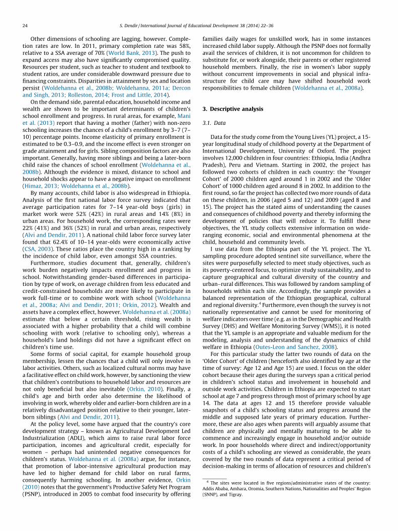
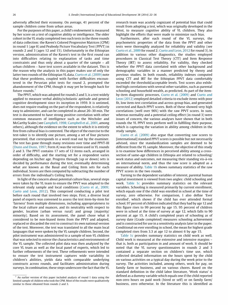
The possible link between children’s endowment and theirschooling and work is first illustrated using simple bivariateanalysis. Fig. 1(1) and (2) present average school enrollment by testscore quintile at ages 12 and 15. Clearly, one can observe a positivetrend in the probability of a child ever/currently enrolling in schooland her quintile test score. At age 12, for instance, the likelihood ofa child in the lowest quintile to have ever been enrolled in school is

8 Although not shown, the interplay between the different types of market work

at the two ‘ages’ is interesting. For instance, the proportion of children who engage

in paid work doubles from age 12 to age 15 (from 4 to 8 percent), but those who

work on the family farm/business actually declines (from about 45 to 39 percent).9 In the questionnaires, ‘low ability’ was not offered among the choices as to why

a child was not enrolled in school.

about 88 percent, while all children in the top quintile are enrolledin school. With the almost monotonic relationship betweencurrent enrollment and test score, the graph at age 12 is probablymost supportive of the hypothesis that a child’s perceivedendowment may indeed be a factor in the parents’ decision toenroll her in school, assuming such a decision overwhelmingly, ifnot solely, rests with the parents. Similarly, by age 15, whereaschildren of all abilities except those in the bottom quintile hadbeen enrolled in school at one time or another, the positivecorrelation between current enrollment and test score is palpable.A quarter of children of the lowest ability, for example, are out ofschool by that age, while the corresponding figure for those in thetop two quintiles is less than 5 percent.

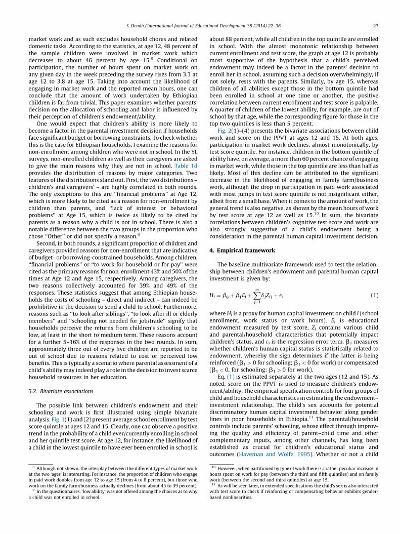
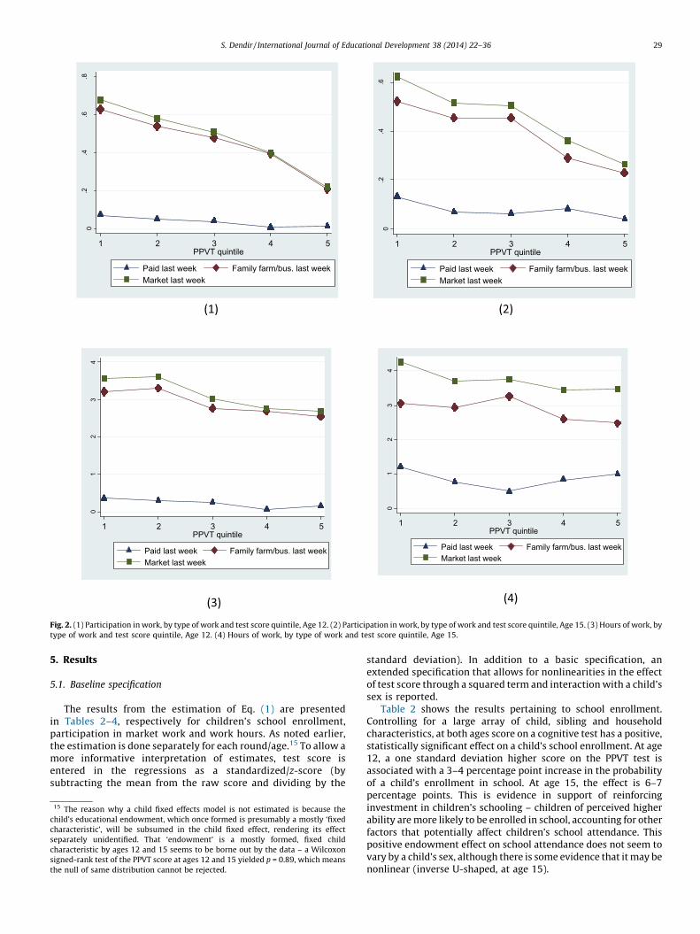
Fig. 2(1)–(4) presents the bivariate associations between childwork and score on the PPVT at ages 12 and 15. At both ages,participation in market work declines, almost monotonically, bytest score quintile. For instance, children in the bottom quintile ofability have, on average, a more than 60 percent chance of engagingin market work, while those in the top quintile are less than half aslikely. Most of this decline can be attributed to the significantdecrease in the likelihood of engaging in family farm/businesswork, although the drop in participation in paid work associatedwith most jumps in test score quintile is not insignificant either,albeit from a small base. When it comes to the amount of work, thegeneral trend is also negative, as shown by the mean hours of workby test score at age 12 as well as 15.10 In sum, the bivariatecorrelations between children’s cognitive test score and work arealso strongly suggestive of a child’s endowment being aconsideration in the parental human capital investment decision.

4. Empirical framework

The baseline multivariate framework used to test the relation-ship between children’s endowment and parental human capitalinvestment is given by:

Hi ¼ b0 þ b1Ei þXm

j¼1

d jZi j þ ei (1)

where Hi is a proxy for human capital investment on child i (schoolenrollment, work status or work hours), Ei is educationalendowment measured by test score, Zi contains various childand parental/household characteristics that potentially impactchildren’s status, and ei is the regression error term. b1 measureswhether children’s human capital status is statistically related toendowment, whereby the sign determines if the latter is beingreinforced (b1 > 0 for schooling; b1 < 0 for work) or compensated(b1 < 0, for schooling; b1 > 0 for work).

Eq. (1) is estimated separately at the two ages (12 and 15). Asnoted, score on the PPVT is used to measure children’s endow-ment/ability. The empirical specification controls for four groups ofchild and household characteristics in estimating the endowment–investment relationship. The child’s sex accounts for potentialdiscriminatory human capital investment behavior along genderlines in poor households in Ethiopia.11 The parental/householdcontrols include parents’ schooling, whose effect through improv-ing the quality and efficiency of parent–child time and othercomplementary inputs, among other channels, has long beenestablished as crucial for children’s educational status andoutcomes (Haveman and Wolfe, 1995). Whether or not a child

10 However, when partitioned by type of work there is a rather peculiar increase in

hours spent on work for pay (between the third and fifth quintiles) and on family

work (between the second and third quintiles) at age 15.11 As will be seen later, in extended specifications the child’s sex is also interacted

with test score to check if reinforcing or compensating behavior exhibits gender-

based nonlinearities.

(1) (2)

.85

.9.9

51

1 2 3 4 5PPVT quintile

Ever enrolled Currently enrolled

.75

.8.8

5.9

.95

1


Ever enrolled Currently enrolled

Fig. 1. (1) School status by test score quintile, Age 12. (2) School status by test score quintile, Age 15.


lives with her parent as the main caregiver may be particularlypertinent in order to realize these benefits, however, therefore thisis controlled for using a dummy variable.

To account for various effects related to household demo-graphics, such as life-cycle position, earnings capabilities andmaternal health and experience, I also include head’s and caregiver’sage, headship status and number of adults residing in the household.The relevant literature has also shown that increased householdresources are associated with many desirable schooling outcomesand decreased child work (Filmer and Pritchett, 1999; Edmonds,2008). For this, a composite index of household wealth andhousehold nondurable expenditure are included as regressors.12

The third set of control variables account for sibling demo-graphics – sibling size, birth order, number of sisters and infantsiblings. Studies have documented that sibling demographics –primarily birth order and sex composition – have importantimplications to a child’s schooling and work status. These aremainly due to cultural influences, changes in parents’ experience,health and earnings over time, evolving patterns in between-siblingcomparative advantage, and fertility choice (Edmonds, 2008). Themajority of evidence from developing countries suggests thatearlier-born children, particularly females, tend to do worse thantheir siblings in various human capital measures. Similarly, havingmore sister siblings is correlated with favorable outcomes (Patrinosand Psacharopoulos, 1997; Garg and Morduch, 1998).

It has been well noted in the literature that children’s health isan important determinant of their school and other activities aswell as their long term human capital accumulation (Strauss andThomas, 1998). A child’s performance on an ability test is alsonaturally associated with her health. To account for this, the fourthset of control variables includes measures of child health. Tomeasure long-term health, variables indicating a child’s ownassessment of her health relative to other children of the same ageare employed. Specifically, the regression includes dummy

12 The reasoning behind including both is that one measures stock (wealth) and

the other flow of resources (expenditure). Specifications that included each

separately were estimated but not reported here, but there were no notable changes

in estimates. The wealth index is a composite index of housing quality, durables and

facilities and takes a value between 0 and 1. A rescaled value (5�) is included in the

regressions.

variables for children who reported having better health andthose who reported having worse health, while the referencecategory is children who said they have the same health as theirpeers.13 To measure short- to medium-term changes in health, avariable indicating whether a child had experienced serious illnesssince the previous round is also included. Finally, as noted in Table1d as well as in the literature, health of parents and otherhousehold members can also impact children’s status (see forexample, Sun and Yao, 2010). In the surveys, households wereasked if illness of the YL child’s parents or other householdmembers was an important event that negatively affected thehousehold’s economy since the previous round. The regressionthus accounts for such shocks using indicator variables for illnessof parents and other household members.

Furthermore, site/community fixed effects are included in allspecifications to control for various supply-side (e.g. school supply,costs and prices) and demand-side (e.g. differential female–malewage rate, youth employment opportunities) factors. A linearprobability model (LPM) is adopted for the estimation of the schoolenrollment and work status regressions. For the child work hoursregressions, which contain a large number of zero values for non-working children, a censored model such as tobit is appropriate.However, tobit estimates also suffer from inconsistency in a fixedeffects framework due to the insufficient statistic problem (tocondition the fixed effects out of the likelihood function). I reporttwo sets of estimates for the work hours regressions: (1) tobitestimates that exclude the community fixed effects (as a baseline),and (2) estimates using Honore’s (1992) semiparametric leastsquares censored fixed effects regression model, which does notimpose any parametric restrictions on the error term. In allregressions, robust standard errors are employed that account forclustering in sample design, which for the YL surveys is at the site/community level.14

13 The YL surveys also asked caregivers to similarly compare their child’s health

relative to other children of the same age. The child and caregiver responses were

highly correlated.14 Nichols and Schaffer (2007) argue that, even in a fixed effects framework,

clustering is desirable to allow for within-cluster correlation of unknown type.

(1) (2)

0.2

.4.6

.8


Paid last week Family farm/bus. last weekMarket last week

0.2

.4.6



(3) (4)

01

23

4



01

23

4



Fig. 2. (1) Participation in work, by type of work and test score quintile, Age 12. (2) Participation in work, by type of work and test score quintile, Age 15. (3) Hours of work, by

type of work and test score quintile, Age 12. (4) Hours of work, by type of work and test score quintile, Age 15.


5. Results

5.1. Baseline specification

The results from the estimation of Eq. (1) are presentedin Tables 2–4, respectively for children’s school enrollment,participation in market work and work hours. As noted earlier,the estimation is done separately for each round/age.15 To allow amore informative interpretation of estimates, test score isentered in the regressions as a standardized/z-score (bysubtracting the mean from the raw score and dividing by the

15 The reason why a child fixed effects model is not estimated is because the

child’s educational endowment, which once formed is presumably a mostly ‘fixed

characteristic’, will be subsumed in the child fixed effect, rendering its effect

separately unidentified. That ‘endowment’ is a mostly formed, fixed child

characteristic by ages 12 and 15 seems to be borne out by the data – a Wilcoxon

signed-rank test of the PPVT score at ages 12 and 15 yielded p = 0.89, which means

the null of same distribution cannot be rejected.

standard deviation). In addition to a basic specification, anextended specification that allows for nonlinearities in the effectof test score through a squared term and interaction with a child’ssex is reported.

Table 2 shows the results pertaining to school enrollment.Controlling for a large array of child, sibling and householdcharacteristics, at both ages score on a cognitive test has a positive,statistically significant effect on a child’s school enrollment. At age12, a one standard deviation higher score on the PPVT test isassociated with a 3–4 percentage point increase in the probabilityof a child’s enrollment in school. At age 15, the effect is 6–7percentage points. This is evidence in support of reinforcinginvestment in children’s schooling – children of perceived higherability are more likely to be enrolled in school, accounting for otherfactors that potentially affect children’s school attendance. Thispositive endowment effect on school attendance does not seem tovary by a child’s sex, although there is some evidence that it may benonlinear (inverse U-shaped, at age 15).

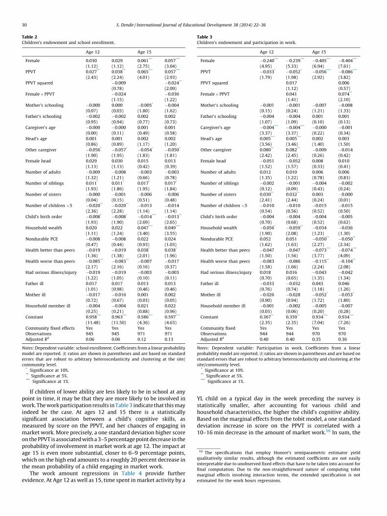
Table 3Children’s endowment and participation in work.

Age 12 Age 15

Female �0.240***

(4.95)

�0.239***

(5.33)

�0.405***

(6.94)

�0.404***

(7.61)

PPVT �0.033*

(1.79)

�0.052*

(1.98)

�0.056***

(2.92)

�0.086***

(3.82)

PPVT squared 0.017

(1.12)

0.006

(0.57)

Female � PPVT 0.041

(1.41)

0.074**

(2.10)

Mother’s schooling �0.001

(0.15)

�0.001

(0.24)

�0.007

(1.21)

�0.008

(1.33)

Father’s schooling �0.004

(1.07)

�0.004

(1.09)

0.001

(0.10)

0.001

(0.13)

Caregiver’s age �0.004***

(3.37)

�0.004***

(3.37)

�0.000

(0.22)

�0.001

(0.34)

Head’s age 0.005***

(3.56)

0.005***

(3.46)

0.002

(1.40)

0.003

(1.50)

Other caregiver 0.080**

(2.42)

0.082**

(2.45)

�0.009

(0.26)

�0.014

(0.42)

Female head �0.051

(1.52)

�0.052*

(1.57)

0.008

(0.33)

0.010

(0.41)

Number of adults 0.012

(1.35)

0.010

(1.22)

0.006

(0.78)

0.006

(0.83)

Number of siblings �0.002

(0.12)

�0.001

(0.09)

�0.004

(0.43)

�0.002

(0.24)

Number of sisters 0.030**

(2.41)

0.032**

(2.44)

0.003

(0.24)

�0.000

(0.01)

Number of children <5 �0.010

(0.54)

�0.010

(0.56)

�0.015

(0.52)

�0.015

(0.50)

Child’s birth order �0.004

(0.70)

�0.004

(0.68)

�0.004

(0.52)

�0.005

(0.62)

Household wealth �0.056*

(1.90)

�0.059**

(2.08)

�0.034

(1.23)

�0.036

(1.30)

Nondurable PCE 0.052

(1.62)

0.051

(1.63)

�0.050**

(2.27)

�0.050**

(2.34)

Health better than peers �0.047

(1.50)

�0.047

(1.56)

�0.073***

(3.77)

�0.074***

(4.09)

Health worse than peers �0.083

(1.58)

�0.086

(1.66)

�0.115**

(2.24)

�0.104**

(2.08)

Had serious illness/injury 0.018

(0.70)

0.016

(0.65)

�0.043

(1.35)

�0.042

(1.34)

Father ill �0.033

(0.76)

�0.032

(0.74)

0.043

(1.18)

0.046

(1.26)

Mother ill �0.026

(0.90)

�0.028

(0.94)

�0.052*

(1.72)

�0.053*

(1.80)

Household member ill �0.001

(0.03)

�0.002

(0.06)

�0.005

(0.20)

�0.007

(0.28)

Constant 0.367**

(2.35)

0.359**

(2.35)

0.934***

(7.04)

0.934***

(7.26)

Community fixed Yes Yes Yes Yes

Observations 944 944 970 970

Adjusted R2 0.40 0.40 0.35 0.36

Notes: Dependent variable: Participation in work. Coefficients from a linear

probability model are reported. jtj ratios are shown in parentheses and are based on

standard errors that are robust to arbitrary heteroscedasticity and clustering at the

site/community level.* Significance at 10%.** Significance at 5%.*** Significance at 1%.

Table 2Children’s endowment and school enrollment.

Age 12 Age 15

Female 0.030

(1.12)

0.029

(1.12)

0.061***

(2.75)

0.057***

(3.04)

PPVT 0.027**

(2.43)

0.038**

(2.24)

0.065***

(4.01)

0.057***

(2.93)

PPVT squared �0.009

(0.78)

�0.024**

(2.09)

Female � PPVT �0.024

(1.15)

�0.036

(1.22)


(0.07)

0.000

(0.03)

�0.005*

(1.80)

�0.004

(1.62)


(0.95)

�0.002

(0.94)

0.002

(0.77)

0.002

(0.73)

Caregiver’s age �0.000

(0.00)

�0.000

(0.11)

0.001

(0.49)

0.001

(0.58)

Head’s age 0.001

(0.86)

0.001

(0.89)

0.002

(1.17)

0.002

(1.20)

Other caregiver �0.056*

(1.90)

�0.057*

(1.95)

�0.054*

(1.83)

�0.050*

(1.81)

Female head 0.029

(1.13)

0.030

(1.13)

0.015

(0.42)

0.013

(0.39)

Number of adults �0.009

(1.32)

�0.008

(1.21)

�0.003

(0.66)

�0.003

(0.78)

Number of siblings 0.011*

(1.93)

0.011*

(1.86)

0.017*

(1.95)

0.017*

(1.84)

Number of sisters �0.000

(0.04)

�0.001

(0.15)

�0.006

(0.51)

�0.006

(0.48)

Number of children <5 �0.020**

(2.36)

�0.020**

(2.28)

�0.013

(1.14)

�0.014

(1.14)

Child’s birth order �0.008*

(1.93)

�0.008*

(1.90)

�0.014***

(2.69)

�0.013**

(2.65)

Household wealth 0.020

(1.11)

0.022

(1.24)

0.047***

(3.40)

0.049***

(3.55)

Nondurable PCE �0.008

(0.47)

�0.008

(0.44)

0.022

(0.93)

0.024

(1.03)


(1.36)

�0.019

(1.38)

0.038*

(2.01)

0.038*

(1.96)

Health worse than peers �0.085**

(2.17)

�0.083**

(2.16)

�0.007

(0.16)

�0.017

(0.37)

Had serious illness/injury �0.019

(1.22)

�0.019

(1.05)

�0.003

(0.10)

�0.003

(0.11)

Father ill 0.017

(1.01)

0.017

(0.98)

0.013

(0.46)

0.013

(0.46)

Mother ill �0.017

(0.72)

�0.016

(0.67)

0.001

(0.03)

0.002

(0.05)


(0.25)

�0.004

(0.21)

0.021

(0.88)

0.022

(0.96)

Constant 0.958***

(11.48)

0.963***

(11.50)

0.586***

(4.36)

0.597***

(4.63)

Community fixed effects Yes Yes Yes Yes


Adjusted R2 0.06 0.06 0.12 0.13

Notes: Dependent variable: school enrollment. Coefficients from a linear probability

model are reported. jtj ratios are shown in parentheses and are based on standard

errors that are robust to arbitrary heteroscedasticity and clustering at the site/

community level.* Significance at 10%.** Significance at 5%.*** Significance at 1%.

16 The specifications that employ Honore’s semiparametric estimator yield

qualitatively similar results, although the estimated coefficients are not easily

interpretable due to unobserved fixed effects that have to be taken into account for

final computation. Due to the non-straightforward nature of computing tobit

marginal effects involving interaction terms, the extended specification is not

estimated for the work hours regressions.


If children of lower ability are less likely to be in school at anypoint in time, it may be that they are more likely to be involved inwork. The work participation results in Table 3 indicate that this mayindeed be the case. At ages 12 and 15 there is a statisticallysignificant association between a child’s cognitive skills, asmeasured by score on the PPVT, and her chances of engaging inmarket work. More precisely, a one standard deviation higher scoreon the PPVT is associated with a 3–5 percentage point decrease in theprobability of involvement in market work at age 12. The impact atage 15 is even more substantial, closer to 6–9 percentage points,which on the high end amounts to a roughly 20 percent decrease inthe mean probability of a child engaging in market work.

The work amount regressions in Table 4 provide furtherevidence. At Age 12 as well as 15, time spent in market activity by a

YL child on a typical day in the week preceding the survey isstatistically smaller, after accounting for various child andhousehold characteristics, the higher the child’s cognitive ability.Based on the marginal effects from the tobit model, a one standarddeviation increase in score on the PPVT is correlated with a10–16 min decrease in the amount of market work.16 In sum, the

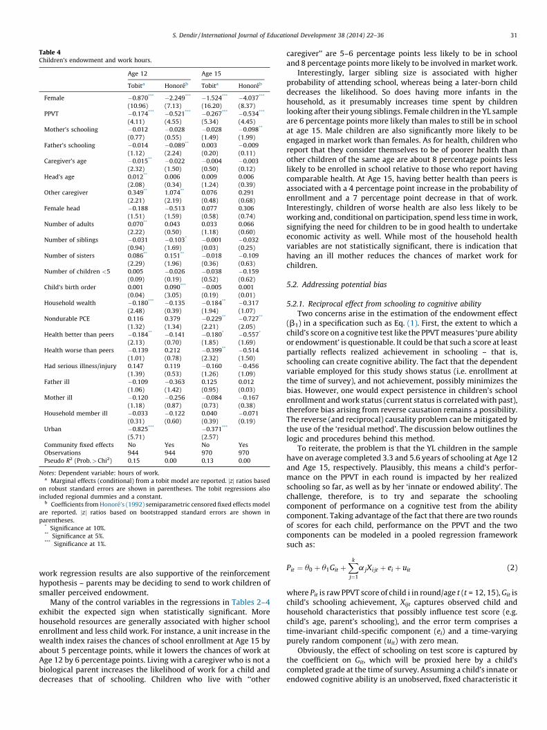
Table 4Children’s endowment and work hours.

Age 12 Age 15

Tobita Honoreb Tobita Honoreb

Female �0.870***

(10.96)

�2.249***

(7.13)

�1.524***

(16.20)

�4.037***

(8.37)

PPVT �0.174***

(4.11)

�0.521***

(4.55)

�0.267***

(5.34)

�0.534***

(4.45)


(0.77)

�0.028

(0.55)

�0.028

(1.49)

�0.098**

(1.99)


(1.12)

�0.089**

(2.24)

0.003

(0.20)

�0.009

(0.11)

Caregiver’s age �0.015**

(2.32)

�0.022

(1.50)

�0.004

(0.50)

�0.003

(0.12)

Head’s age 0.012**

(2.08)

0.006

(0.34)

0.009

(1.24)

0.006

(0.39)


(2.21)

1.074**

(2.19)

0.076

(0.48)

0.291

(0.68)


(1.51)

�0.513

(1.59)

0.077

(0.58)

0.306

(0.74)

Number of adults 0.070**

(2.22)

0.043

(0.50)

0.033

(1.18)

0.066

(0.60)


(0.94)

�0.103*

(1.69)

�0.001

(0.03)

�0.032

(0.25)

Number of sisters 0.086**

(2.29)

0.151**

(1.96)

�0.018

(0.36)

�0.109

(0.63)

Number of children <5 0.005

(0.09)

�0.026

(0.19)

�0.038

(0.52)

�0.159

(0.62)

Child’s birth order 0.001

(0.04)

0.090***

(3.05)

�0.005

(0.19)

0.001

(0.01)

Household wealth �0.180***

(2.48)

�0.135

(0.39)

�0.184**

(1.94)

�0.317

(1.07)


(1.32)

0.379

(1.34)

�0.229**

(2.21)

�0.727**

(2.05)

Health better than peers �0.184**

(2.13)

�0.141

(0.70)

�0.180*

(1.85)

�0.557*

(1.69)


(1.01)

0.212

(0.78)

�0.399**

(2.32)

�0.514

(1.50)


(1.39)

0.119

(0.53)

�0.160

(1.26)

�0.456

(1.09)

Father ill �0.109

(1.06)

�0.363

(1.42)

0.125

(0.95)

0.012

(0.03)

Mother ill �0.120

(1.18)

�0.256

(0.87)

�0.084

(0.73)

�0.167

(0.38)


(0.31)

�0.122

(0.60)

0.040

(0.39)

�0.071

(0.19)

Urban �0.825***

(5.71)

�0.371***

(2.57)

Community fixed effects No Yes No Yes


Pseudo R2 (Prob. > Chi2) 0.15 0.00 0.13 0.00

Notes: Dependent variable: hours of work.a Marginal effects (conditional) from a tobit model are reported. jzj ratios based

on robust standard errors are shown in parentheses. The tobit regressions also

included regional dummies and a constant.b Coefficients from Honore’s (1992) semiparametric censored fixed effects model

are reported. jzj ratios based on bootstrapped standard errors are shown in

parentheses.* Significance at 10%.** Significance at 5%.*** Significance at 1%.


work regression results are also supportive of the reinforcementhypothesis – parents may be deciding to send to work children ofsmaller perceived endowment.

Many of the control variables in the regressions in Tables 2–4exhibit the expected sign when statistically significant. Morehousehold resources are generally associated with higher schoolenrollment and less child work. For instance, a unit increase in thewealth index raises the chances of school enrollment at Age 15 byabout 5 percentage points, while it lowers the chances of work atAge 12 by 6 percentage points. Living with a caregiver who is not abiological parent increases the likelihood of work for a child anddecreases that of schooling. Children who live with ‘‘other

caregiver’’ are 5–6 percentage points less likely to be in schooland 8 percentage points more likely to be involved in market work.

Interestingly, larger sibling size is associated with higherprobability of attending school, whereas being a later-born childdecreases the likelihood. So does having more infants in thehousehold, as it presumably increases time spent by childrenlooking after their young siblings. Female children in the YL sampleare 6 percentage points more likely than males to still be in schoolat age 15. Male children are also significantly more likely to beengaged in market work than females. As for health, children whoreport that they consider themselves to be of poorer health thanother children of the same age are about 8 percentage points lesslikely to be enrolled in school relative to those who report havingcomparable health. At Age 15, having better health than peers isassociated with a 4 percentage point increase in the probability ofenrollment and a 7 percentage point decrease in that of work.Interestingly, children of worse health are also less likely to beworking and, conditional on participation, spend less time in work,signifying the need for children to be in good health to undertakeeconomic activity as well. While most of the household healthvariables are not statistically significant, there is indication thathaving an ill mother reduces the chances of market work forchildren.

5.2. Addressing potential bias

5.2.1. Reciprocal effect from schooling to cognitive ability

Two concerns arise in the estimation of the endowment effect(b1) in a specification such as Eq. (1). First, the extent to which achild’s score on a cognitive test like the PPVT measures ‘pure abilityor endowment’ is questionable. It could be that such a score at leastpartially reflects realized achievement in schooling – that is,schooling can create cognitive ability. The fact that the dependentvariable employed for this study shows status (i.e. enrollment atthe time of survey), and not achievement, possibly minimizes thebias. However, one would expect persistence in children’s schoolenrollment and work status (current status is correlated with past),therefore bias arising from reverse causation remains a possibility.The reverse (and reciprocal) causality problem can be mitigated bythe use of the ‘residual method’. The discussion below outlines thelogic and procedures behind this method.

To reiterate, the problem is that the YL children in the samplehave on average completed 3.3 and 5.6 years of schooling at Age 12and Age 15, respectively. Plausibly, this means a child’s perfor-mance on the PPVT in each round is impacted by her realizedschooling so far, as well as by her ‘innate or endowed ability’. Thechallenge, therefore, is to try and separate the schoolingcomponent of performance on a cognitive test from the abilitycomponent. Taking advantage of the fact that there are two roundsof scores for each child, performance on the PPVT and the twocomponents can be modeled in a pooled regression frameworksuch as:

Pit ¼ u0 þ u1Git þXk

j¼1

a jXi jt þ ei þ uit (2)

where Pit is raw PPVT score of child i in round/age t (t = 12, 15), Git ischild’s schooling achievement, Xijt captures observed child andhousehold characteristics that possibly influence test score (e.g.child’s age, parent’s schooling), and the error term comprises atime-invariant child-specific component (ei) and a time-varyingpurely random component (uit) with zero mean.

Obviously, the effect of schooling on test score is captured bythe coefficient on Git, which will be proxied here by a child’scompleted grade at the time of survey. Assuming a child’s innate orendowed cognitive ability is an unobserved, fixed characteristic it

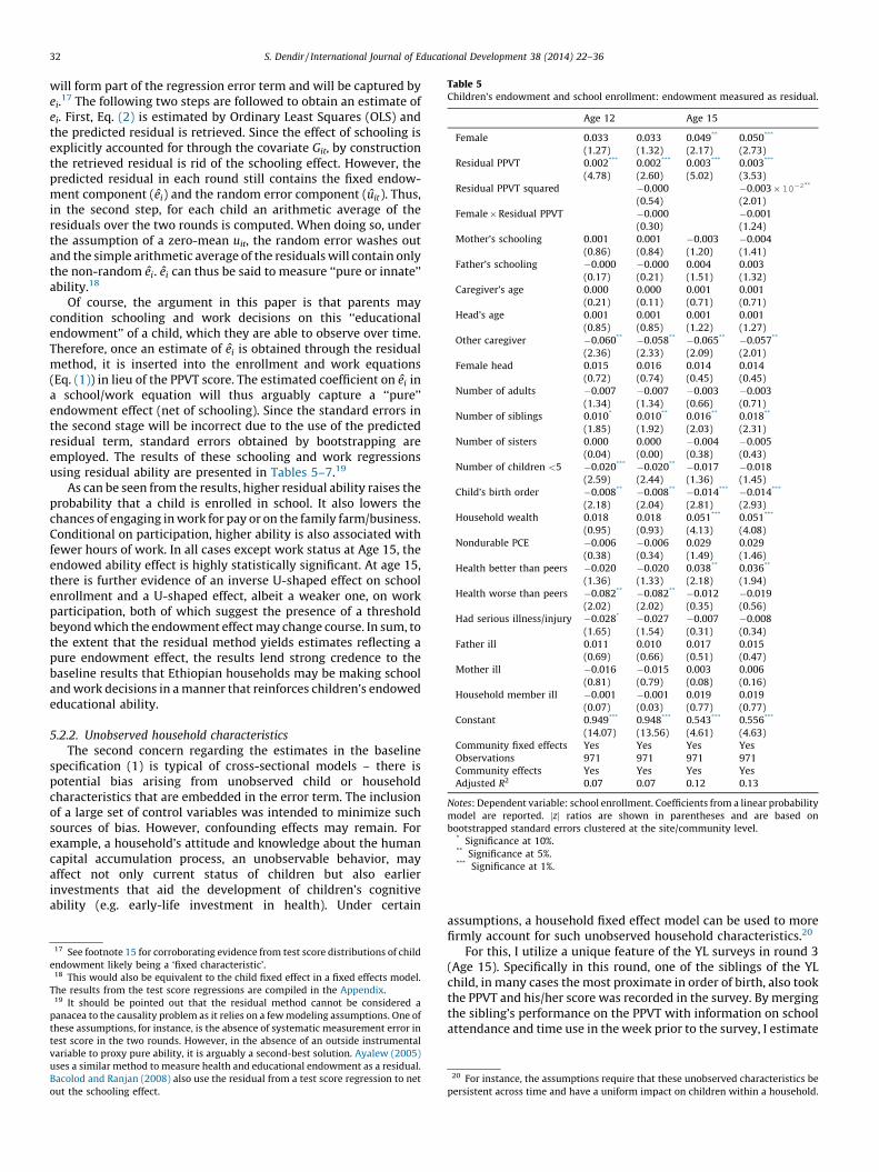
Table 5Children’s endowment and school enrollment: endowment measured as residual.

Age 12 Age 15

Female 0.033

(1.27)

0.033

(1.32)

0.049**

(2.17)

0.050***

(2.73)

Residual PPVT 0.002***

(4.78)

0.002***

(2.60)

0.003***

(5.02)

0.003***

(3.53)

Residual PPVT squared �0.000

(0.54)

�0.003 � 10�2**

(2.01)

Female � Residual PPVT �0.000

(0.30)

�0.001

(1.24)

Mother’s schooling 0.001

(0.86)

0.001

(0.84)

�0.003

(1.20)

�0.004

(1.41)


(0.17)

�0.000

(0.21)

0.004

(1.51)

0.003

(1.32)

Caregiver’s age 0.000

(0.21)

0.000

(0.11)

0.001

(0.71)

0.001

(0.71)

Head’s age 0.001

(0.85)

0.001

(0.85)

0.001

(1.22)

0.001

(1.27)

Other caregiver �0.060**

(2.36)

�0.058**

(2.33)

�0.065**

(2.09)

�0.057**

(2.01)

Female head 0.015

(0.72)

0.016

(0.74)

0.014

(0.45)

0.014

(0.45)

Number of adults �0.007

(1.34)

�0.007

(1.34)

�0.003

(0.66)

�0.003

(0.71)

Number of siblings 0.010*

(1.85)

0.010**

(1.92)

0.016**

(2.03)

0.018**

(2.31)

Number of sisters 0.000

(0.04)

0.000

(0.00)

�0.004

(0.38)

�0.005

(0.43)

Number of children <5 �0.020***

(2.59)

�0.020**

(2.44)

�0.017

(1.36)

�0.018

(1.45)

Child’s birth order �0.008**

(2.18)

�0.008**

(2.04)

�0.014***

(2.81)

�0.014***

(2.93)

Household wealth 0.018

(0.95)

0.018

(0.93)

0.051***

(4.13)

0.051***

(4.08)

Nondurable PCE �0.006

(0.38)

�0.006

(0.34)

0.029

(1.49)

0.029

(1.46)


(1.36)

�0.020

(1.33)

0.038**

(2.18)

0.036**

(1.94)

Health worse than peers �0.082**

(2.02)

�0.082**

(2.02)

�0.012

(0.35)

�0.019

(0.56)

Had serious illness/injury �0.028*

(1.65)

�0.027

(1.54)

�0.007

(0.31)

�0.008

(0.34)

Father ill 0.011

(0.69)

0.010

(0.66)

0.017

(0.51)

0.015

(0.47)

Mother ill �0.016

(0.81)

�0.015

(0.79)

0.003

(0.08)

0.006

(0.16)


(0.07)

�0.001

(0.03)

0.019

(0.77)

0.019

(0.77)

Constant 0.949***

(14.07)

0.948***

(13.56)

0.543***

(4.61)

0.556***

(4.63)



Community effects Yes Yes Yes Yes

Adjusted R2 0.07 0.07 0.12 0.13

Notes: Dependent variable: school enrollment. Coefficients from a linear probability

model are reported. jzj ratios are shown in parentheses and are based on

bootstrapped standard errors clustered at the site/community level.* Significance at 10%.** Significance at 5%.*** Significance at 1%.


will form part of the regression error term and will be captured byei.

17 The following two steps are followed to obtain an estimate ofei. First, Eq. (2) is estimated by Ordinary Least Squares (OLS) andthe predicted residual is retrieved. Since the effect of schooling isexplicitly accounted for through the covariate Git, by constructionthe retrieved residual is rid of the schooling effect. However, thepredicted residual in each round still contains the fixed endow-ment component (ei) and the random error component (uit). Thus,in the second step, for each child an arithmetic average of theresiduals over the two rounds is computed. When doing so, underthe assumption of a zero-mean uit, the random error washes outand the simple arithmetic average of the residuals will contain onlythe non-random ei. ei can thus be said to measure ‘‘pure or innate’’ability.18

Of course, the argument in this paper is that parents maycondition schooling and work decisions on this ‘‘educationalendowment’’ of a child, which they are able to observe over time.Therefore, once an estimate of ei is obtained through the residualmethod, it is inserted into the enrollment and work equations(Eq. (1)) in lieu of the PPVT score. The estimated coefficient on ei ina school/work equation will thus arguably capture a ‘‘pure’’endowment effect (net of schooling). Since the standard errors inthe second stage will be incorrect due to the use of the predictedresidual term, standard errors obtained by bootstrapping areemployed. The results of these schooling and work regressionsusing residual ability are presented in Tables 5–7.19

As can be seen from the results, higher residual ability raises theprobability that a child is enrolled in school. It also lowers thechances of engaging in work for pay or on the family farm/business.Conditional on participation, higher ability is also associated withfewer hours of work. In all cases except work status at Age 15, theendowed ability effect is highly statistically significant. At age 15,there is further evidence of an inverse U-shaped effect on schoolenrollment and a U-shaped effect, albeit a weaker one, on workparticipation, both of which suggest the presence of a thresholdbeyond which the endowment effect may change course. In sum, tothe extent that the residual method yields estimates reflecting apure endowment effect, the results lend strong credence to thebaseline results that Ethiopian households may be making schooland work decisions in a manner that reinforces children’s endowededucational ability.

5.2.2. Unobserved household characteristics

The second concern regarding the estimates in the baselinespecification (1) is typical of cross-sectional models – there ispotential bias arising from unobserved child or householdcharacteristics that are embedded in the error term. The inclusionof a large set of control variables was intended to minimize suchsources of bias. However, confounding effects may remain. Forexample, a household’s attitude and knowledge about the humancapital accumulation process, an unobservable behavior, mayaffect not only current status of children but also earlierinvestments that aid the development of children’s cognitiveability (e.g. early-life investment in health). Under certain

17 See footnote 15 for corroborating evidence from test score distributions of child

endowment likely being a ‘fixed characteristic’.18 This would also be equivalent to the child fixed effect in a fixed effects model.

The results from the test score regressions are compiled in the Appendix.19 It should be pointed out that the residual method cannot be considered a

panacea to the causality problem as it relies on a few modeling assumptions. One of

these assumptions, for instance, is the absence of systematic measurement error in

test score in the two rounds. However, in the absence of an outside instrumental

variable to proxy pure ability, it is arguably a second-best solution. Ayalew (2005)

uses a similar method to measure health and educational endowment as a residual.

Bacolod and Ranjan (2008) also use the residual from a test score regression to net

out the schooling effect.

assumptions, a household fixed effect model can be used to morefirmly account for such unobserved household characteristics.20

For this, I utilize a unique feature of the YL surveys in round 3(Age 15). Specifically in this round, one of the siblings of the YLchild, in many cases the most proximate in order of birth, also tookthe PPVT and his/her score was recorded in the survey. By mergingthe sibling’s performance on the PPVT with information on schoolattendance and time use in the week prior to the survey, I estimate

20 For instance, the assumptions require that these unobserved characteristics be

persistent across time and have a uniform impact on children within a household.

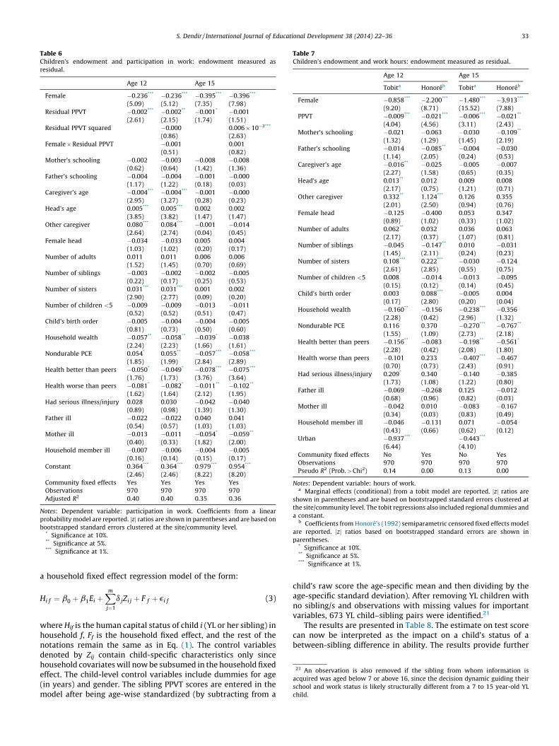
Table 6Children’s endowment and participation in work: endowment measured as

residual.

Age 12 Age 15

Female �0.236***

(5.09)

�0.236***

(5.12)

�0.395***

(7.35)

�0.396***

(7.98)

Residual PPVT �0.002***

(2.61)

�0.002**

(2.15)

�0.001*

(1.74)

�0.001

(1.51)

Residual PPVT squared �0.000

(0.86)

0.006 � 10�2***

(2.63)

Female � Residual PPVT �0.001

(0.51)

0.001

(0.82)


(0.62)

�0.003

(0.64)

�0.008

(1.42)

�0.008

(1.36)


(1.17)

�0.004

(1.22)

�0.001

(0.18)

�0.000

(0.03)

Caregiver’s age �0.004***

(2.95)

�0.004***

(3.27)

�0.001

(0.28)

�0.000

(0.23)

Head’s age 0.005***

(3.85)

0.005***

(3.82)

0.002

(1.47)

0.002

(1.47)

Other caregiver 0.080***

(2.64)

0.084***

(2.74)

�0.001

(0.04)

�0.014

(0.45)


(1.03)

�0.033

(1.02)

0.005

(0.20)

0.004

(0.17)

Number of adults 0.011

(1.52)

0.011

(1.45)

0.006

(0.70)

0.006

(0.69)


(0.22)

�0.002

(0.17)

�0.002

(0.25)

�0.005

(0.53)

Number of sisters 0.031***

(2.90)

0.031***

(2.77)

0.001

(0.09)

0.002

(0.20)

Number of children <5 �0.009

(0.52)

�0.009

(0.52)

�0.013

(0.51)

�0.011

(0.47)


(0.81)

�0.004

(0.73)

�0.004

(0.50)

�0.005

(0.60)

Household wealth �0.057**

(2.24)

�0.058**

(2.23)

�0.039*

(1.66)

�0.038

(1.61)

Nondurable PCE 0.054*

(1.85)

0.055**

(1.99)

�0.057***

(2.84)

�0.058***

(2.89)

Health better than peers �0.050*

(1.76)

�0.049*

(1.73)

�0.078***

(3.76)

�0.075***

(3.64)

Health worse than peers �0.081*

(1.62)

�0.082*

(1.64)

�0.011**

(2.12)

�0.102**

(1.95)


(0.89)

0.030

(0.98)

�0.042

(1.39)

�0.040

(1.30)

Father ill �0.022

(0.54)

�0.022

(0.57)

0.040

(1.03)

0.041

(1.03)

Mother ill �0.013

(0.40)

�0.011

(0.33)

�0.054*

(1.82)

�0.059**

(2.00)


(0.16)

�0.006

(0.14)

�0.004

(0.15)

�0.005

(0.17)

Constant 0.364***

(2.46)

0.364***

(2.46)

0.979***

(8.22)

0.954***

(8.20)



Adjusted R2 0.40 0.40 0.35 0.36

Notes: Dependent variable: participation in work. Coefficients from a linear

probability model are reported. jzj ratios are shown in parentheses and are based on

bootstrapped standard errors clustered at the site/community level.* Significance at 10%.** Significance at 5%.*** Significance at 1%.

Table 7Children’s endowment and work hours: endowment measured as residual.

Age 12 Age 15

Tobita Honoreb Tobita Honoreb

Female �0.858***

(9.20)

�2.200***

(8.71)

�1.480***

(15.52)

�3.913***

(7.88)

PPVT �0.009***

(4.04)

�0.021***

(4.56)

�0.006***

(3.11)

�0.021**

(2.43)


(1.32)

�0.063

(1.29)

�0.030

(1.45)

�0.109**

(2.19)


(1.14)

�0.085**

(2.05)

�0.004

(0.24)

�0.030

(0.53)

Caregiver’s age �0.016**

(2.27)

�0.025

(1.58)

�0.005

(0.65)

�0.007

(0.35)

Head’s age 0.013**

(2.17)

0.012

(0.75)

0.009

(1.21)

0.008

(0.71)


(2.01)

1.124***

(2.50)

0.126

(0.94)

0.355

(0.76)


(0.89)

�0.400

(1.02)

0.053

(0.33)

0.347

(1.02)

Number of adults 0.062**

(2.17)

0.032

(0.37)

0.036

(1.07)

0.063

(0.81)


(1.45)

�0.147**

(2.11)

0.010

(0.24)

�0.031

(0.23)

Number of sisters 0.108***

(2.61)

0.222***

(2.85)

�0.030

(0.55)

�0.124

(0.75)

Number of children <5 0.008

(0.15)

�0.014

(0.12)

�0.013

(0.14)

�0.095

(0.45)

Child’s birth order 0.003

(0.17)

0.088***

(2.80)

�0.005

(0.20)

0.004

(0.04)

Household wealth �0.160**

(2.28)

�0.156

(0.42)

�0.238***

(2.96)

�0.356

(1.32)


(1.55)

0.370

(1.09)

�0.270***

(2.73)

�0.767**

(2.18)

Health better than peers �0.156**

(2.28)

�0.083

(0.42)

�0.198**

(2.08)

�0.561*

(1.80)


(0.70)

0.233

(0.73)

�0.407***

(2.43)

�0.467

(0.91)

Had serious illness/injury 0.209*

(1.73)

0.340

(1.08)

�0.140

(1.22)

�0.385

(0.80)

Father ill �0.069

(0.68)

�0.268

(0.96)

0.125

(0.82)

�0.012

(0.03)

Mother ill �0.042

(0.34)

0.010

(0.03)

�0.083

(0.83)

�0.167

(0.49)


(0.43)

�0.131

(0.66)

0.071

(0.62)

�0.054

(0.12)

Urban �0.937***

(6.44)

�0.443***

(4.10)

Community fixed effects No Yes No Yes


Pseudo R2 (Prob. > Chi2) 0.14 0.00 0.13 0.00

Notes: Dependent variable: hours of work.a Marginal effects (conditional) from a tobit model are reported. jzj ratios are

shown in parentheses and are based on bootstrapped standard errors clustered at

the site/community level. The tobit regressions also included regional dummies and

a constant.b Coefficients from Honore’s (1992) semiparametric censored fixed effects model

are reported. jzj ratios based on bootstrapped standard errors are shown in

parentheses.* Significance at 10%.** Significance at 5%.*** Significance at 1%.

21 An observation is also removed if the sibling from whom information is

acquired was aged below 7 or above 16, since the decision dynamic guiding their

school and work status is likely structurally different from a 7 to 15 year-old YL

child.


a household fixed effect regression model of the form:

Hi f ¼ b0 þ b1Ei þXm

j¼1

d jZi j þ F f þ ei f (3)

where Hif is the human capital status of child i (YL or her sibling) inhousehold f, Ff is the household fixed effect, and the rest of thenotations remain the same as in Eq. (1). The control variablesdenoted by Zij contain child-specific characteristics only sincehousehold covariates will now be subsumed in the household fixedeffect. The child-level control variables include dummies for age(in years) and gender. The sibling PPVT scores are entered in themodel after being age-wise standardized (by subtracting from a

child’s raw score the age-specific mean and then dividing by theage-specific standard deviation). After removing YL children withno sibling/s and observations with missing values for importantvariables, 673 YL child–sibling pairs were identified.21

The results are presented in Table 8. The estimate on test scorecan now be interpreted as the impact on a child’s status of abetween-sibling difference in ability. The results provide further

Table 8Children’s endowment, school enrollment and work: household fixed effects estimates using sibling pairs.

School enrollmenta Work statusb Work hoursc

Female 0.057***

(2.80)

0.053***

(2.59)

�0.430***

(15.97)

�0.425***

(15.91)

�3.936***

(11.66)

�3.909***

(10.92)

PPVT 0.046***

(2.90)

0.056***

(2.78)

�0.046**

(2.20)

�0.051*

(1.91)

�0.611***

(3.29)

�0.060

(0.23)

PPVT squared �0.023**

(2.15)

0.039***

(2.75)

0.437***

(2.93)

Female � PPVT �0.067***

(3.28)

0.084***

(3.16)

�0.094

(0.28)

Constant 0.329***

(2.96)

0.347

(3.13)

0.687***

(4.73)

0.654

(4.53)

Age dummies Yes Yes Yes Yes Yes Yes

HH fixed effects Yes Yes Yes Yes Yes Yes

Observations 1346 1346 1343 1343 1343 1343

F stat. (Chi2) 5.78 6.14 24.09 22.16 165.04 200.23

Prob. > F (Chi2) 0.000 0.000 0.000 0.000 0.000 0.000

Notes: jtj ratios are shown in parentheses.a ,b Coefficients from a linear probability model are reported.c Coefficients from Honore’s (1992) semiparametric censored fixed effects model are reported.* Significance at 10%.** Significance at 5%.*** Significance at 1%.


support to the evidence in the baseline cross-sectional regressionsof household investment that reinforces differences in children’sperceived ability. A higher ability child is more likely to be inschool, less likely to work and works fewer hours than her lowerscoring sibling. Given the significance of the squared andinteracted terms, again there is evidence of a non-linear effecton child outcomes that was apparent from the earlier results. Forexample, the results suggest that within a household, the abilityeffect may be smaller for female children.

6. Discussion

Using data from a sample that provides a balanced representa-tion of Ethiopia’s geographical, cultural and regional diversity, theanalyses in this paper establish a strong relationship betweenchildren’s cognitive ability and their school and work status.Specifically, the results show that children that score higher on anability test are more likely to be enrolled in school and less likely towork. How do these results stack up against existing evidence? Asnoted earlier, the literature that examines the relationship betweencognitive ability, measured directly using test scores, and invest-ment in children’s human capital is relatively scant. However, theresults in this paper largely conform to the few existing findings.

For example, Ayalew (2005) had reported, using data from avillage in Ethiopia, children who score higher on the Raven’sProgressive Matrices test were more likely to be enrolled in school,which he presents as evidence that households allocate educationalinputs in a reinforcing manner. In corroborating the interpretation,he notes that when parents were asked who would they choose ifthey had the resources to send only one child to school, the mostcommon response was ‘the child who was good at schoolwork’.Bacolod and Ranjan (2008) showed that among a sample of childrenin the Cebu metropolitan area, those who scored higher on an IQ testwere more likely to be in school and less likely to be idle. Glick andSahn (2010) examined test score data from 2nd graders in Senegaland reported that higher ability then was strongly correlated withschooling progression seven years later, which they suggest may bedue to parental investment driven by higher potential returns. Akreshet al. (2012a) tested the ability/endowment hypothesis in a siblingrivalry framework, which stipulates that given market and resourceconstraints, children with fewer siblings of a favored characteristicwill be better off. Their analysis using data from a province in BurkinaFaso indicates reinforcing educational investment. For example, a

child who has one sibling of higher ability – measured by score on theCPM – was 15% less likely to be currently enrolled in school. Evidencelinking ability with children’s work status is even more scarce,although Bacolod and Ranjan (2008) and, in a recent paper, Akreshet al. (2012b) had also documented that higher cognitive abilitylowers the probability of child labor.

In a broader context, the results in this paper are also largelyconsistent with the well-noted relationship in the academicliterature between investment in children’s health, nutrition andeducation in the early years and their status and outcomes inprimary school and beyond (see for example, Glewwe et al., 2001;Grantham-McGregor et al., 2007). The main conduit for this link isthe degree of cognitive development, for which the first few yearsof life are crucial. In the literature for developing countries, forinstance, cognitive ability at preschool and around grade 1 is foundto predict school enrollment and achievement later in life (Liddelland Rae, 2001; Stith et al., 2003). Using YL data, Sanchez (2009)links early nutrition and health to later cognitive outcomes amongPeruvian children. Woldehanna (2011b), also using the Ethiopia partof YL data, shows early educational investment in the form ofpreschool attendance improves cognitive performance of children atages 5 and 8. As such, the emphasis in this literature is on the direct

role that reduced cognitive ability can play in hampering children’shuman capital accumulation down the years. Distinctly, the resultsin this paper suggest an indirect role since, in the face of income andother constraints, households may decide to send children ofperceived lower ability to work instead of school. This indirect routecan thus perpetuate and exacerbate the negative effects on long-term human capital accumulation of children. The evidencepresented is also particularly pertinent to Ethiopia since the countryregisters a very high proportion of children under 5 years (60% ormore, by some accounts) who face multiple risks to their cognitiveand other development (see Grantham-McGregor et al., 2007).

7. Conclusion and policy implications

The overwhelming evidence that emerges from the analyses inthis paper using data on a cohort of children from Ethiopia pointstoward a pattern of household investment in human capital thatcomplements initial differences in children’s educational endow-ment. The related literature suggests this is largely due toinvestment behavior that seeks higher future marginal returns.It can also be due to contemporaneous efficiencies in human

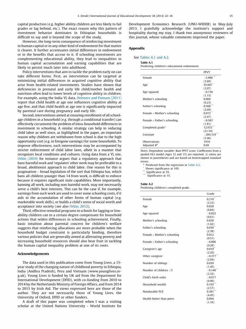
Table A.1Predicting children’s educational endowment.

PPVT

Female �5.986***

(3.69)

Age 35.607**

(2.07)

Age squared �0.730

(1.15)


(0.23)

Father’s schooling 0.568***

(2.69)

Female � Mother’s schooling 0.972***

(2.47)

Female � Father’s schooling �0.583*

(1.81)

Completed gradea 12.033***

(21.54)

Constant �284.310***

(2.46)

Observations 1916

Adjusted R2 0.69

Notes: Dependent variable: Raw PPVT score. Coefficients from a

pooled OLS model (Ages 12 and 15) are reported. jzj ratios are

shown in parentheses and are based on bootstrapped standard

errors.a Predicted from the regression in Table A.2.* Shows significance at 10%.** Significance at 5%.*** Significance at 1%.

Table A.2Predicting children’s completed grade.

Grade

Female 0.210**

(2.23)

Age 0.828

(0.84)

Age squared �0.022

(0.61)


(1.62)

Father’s schooling 0.036**

(2.38)

Female � Mother’s schooling 0.012

(0.51)

Female � Father’s schooling �0.006

(0.28)

Caregiver’s age 0.010**

(2.20)

Other caregiver �0.377***

(2.94)

Number of siblings 0.039

(1.45)

Number of children <5 �0.149**

(2.32)


(0.90)

Household wealth 0.193***

(2.57)

Nondurable PCE 0.381***

(4.45)

Health better than peers 0.094

(1.16)


capital production (e.g. higher ability children are less likely to failgrades or lag behind, etc.). The exact reason why this pattern ofinvestment behavior dominates in Ethiopian households isdifficult to say and is beyond the scope of the study.

However, the long-term consequence of reinforcing investmentin human capital or in any other kind of endowment for that matteris clearer. It further accentuates initial differences in endowmentor in the benefits that accrue to it. If schooling investments arecomplementing educational ability, they lead to inequalities inhuman capital accumulation and earning capabilities that arelikely to persist much later into adulthood.

Policy interventions that aim to tackle the problem early on cantake different forms. First, an intervention can be targeted atminimizing initial differences in acquired cognitive ability thatarise from health-related investments. Studies have shown thatdeficiencies in prenatal and early life child/mother health andnutrition often lead to lower levels of cognitive ability in children.For example, using the India YL data, Helmers and Patnam (2011)report that child health at age one influences cognitive ability atage five, and that child health at age one is significantly impactedby parental care during pregnancy and early life.

Second, interventions aimed at ensuring enrollment of all school-age children in a household (e.g. through a conditional transfer) caneffectively circumvent the problem of intra-household differences ininvestment in schooling. A similar strategy can help in reducingchild labor as well since, as highlighted in the paper, an importantreason why children are withdrawn from school is due to the highopportunity cost (e.g. in foregone earnings) for some households. Toimprove effectiveness, such interventions may be accompanied bystricter enforcement of child labor laws, albeit in a manner thatrecognizes local conditions and cultures. Using data from a YL site,Orkin (2010) for instance argues that a regulatory approach thatbans harmful work and ‘regulates’ other work may be preferable to abroad, abolitionist approach to child labor. One reason for this ispragmatism – broad legislation of the sort that Ethiopia has, whichbans all children younger than 14 from work, is difficult to enforcebecause it requires significant state capabilities. More importantly,banning all work, including non-harmful work, may not necessarilyserve a child’s best interests. This can be the case if, for example,earnings from such work are used to cover some schooling costs, if itaids in the accumulation of other forms of human capital (e.g.marketable work skills), or builds a child’s sense of social worth andacceptance into society (see also Orkin, 2012).

Third, effective remedial programs in schools for lagging or low-ability children can to a certain degree compensate for householdactions that widen differences in schooling achievement. Finally,basic intuition about parental concern for children’s welfaresuggests that reinforcing allocations are more probable when thehousehold budget constraint is particularly binding, thereforevarious policies that are generally aimed at alleviating poverty andincreasing household resources should also bear fruit in tacklingthe human capital inequality problem at one of its roots.

Acknowledgements

The data used in this publication come from Young Lives, a 15-year study of the changing nature of childhood poverty in Ethiopia,India (Andhra Pradesh), Peru and Vietnam (www.younglives.or-g.uk). Young Lives is funded by UK aid from the Department forInternational Development (DFID), with co-funding from 2010 to2014 by the Netherlands Ministry of Foreign Affairs, and from 2014to 2015 by Irish Aid. The views expressed here are those of theauthor. They are not necessarily those of Young Lives, theUniversity of Oxford, DFID or other funders.

A draft of this paper was completed when I was a visitingscholar at the United Nations University - World Institute for

Development Economics Research (UNU-WIDER) in May-July2013. I gratefully acknowledge the institute’s support andhospitality during my stay. I thank two anonymous reviewers ofthis journal, whose valuable comments improved the paper.

Appendix

See Tables A.1 and A.2.

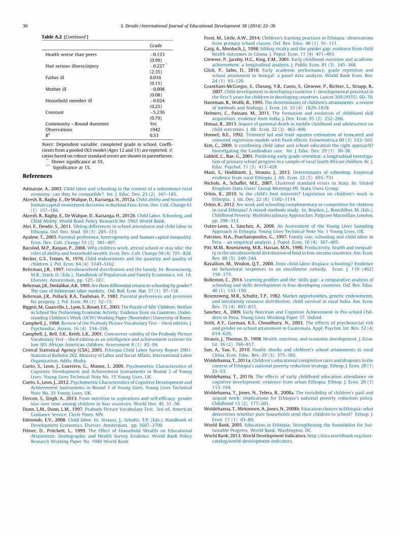
Table A.2 (Continued )

Grade


(0.99)

Had serious illness/injury �0.227**

(2.35)

Father ill 0.016

(0.15)

Mother ill �0.008

(0.08)


(0.25)

Constant �5.236

(0.79)

Community � Round dummies Yes

Observations 1942

R2 0.53

Notes: Dependent variable: completed grade in school. Coeffi-

cients from a pooled OLS model (Ages 12 and 15) are reported. jtjratios based on robust standard errors are shown in parentheses.

** Shows significance at 5%.*** Significance at 1%.


References

Admassie, A., 2003. Child labor and schooling in the context of a subsistence ruraleconomy: can they be compatible? Int. J. Educ. Dev. 23 (2) 167–185.

Akresh, R., Bagby, E., De Walque, D., Kazianga, H., 2012a. Child ability and householdhuman capital investment decisions in Burkina Faso. Econ. Dev. Cult. Change 61(1) 157–186.

Akresh, R., Bagby, E., De Walque, D., Kazianga, H., 2012b. Child Labor, Schooling, andChild Ability. World Bank Policy Research No. 5965 World Bank.

Alvi, E., Dendir, S., 2011. Sibling differences in school attendance and child labor inEthiopia. Oxf. Dev. Stud. 39 (3) 285–313.

Ayalew, T., 2005. Parental preference, heterogeneity and human capital inequality.Econ. Dev. Cult. Change 53 (2) 381–407.

Bacolod, M.P., Ranjan, P., 2008. Why children work, attend school or stay idle: theroles of ability and household wealth. Econ. Dev. Cult. Change 56 (4) 791–828.

Becker, G.S., Tomes, N., 1976. Child endowments and the quantity and quality ofchildren. J. Pol. Econ. 84 (4) S143–S162.

Behrman, J.R., 1997. Intrahousehold distribution and the family. In: Rosenzweig,M.R., Stark, O. (Eds.), Handbook of Population and Family Economics, vol. 1A.Elsevier, Amsterdam, pp. 125–187.

Behrman, J.R., Deolalikar, A.B., 1995. Are there differential returns to schooling by gender?The case of Indonesian labor markets. Oxf. Bull. Econ. Stat. 57 (1) 97–118.

Behrman, J.R., Pollack, R.A., Taubman, P., 1982. Parental preferences and provisionfor progeny. J. Pol. Econ. 90 (1) 52–73.

Biggeri, M., Guarcello, L., Lyon, S., Rosati, F.C., 2003. The Puzzle of ‘Idle’ Children: Neitherin School Nor Performing Economic Activity: Evidence from six Countries. Under-standing Children’s Work (UCW) Working Paper (November) University of Rome.

Campbell, J., 1998. Review of the Peabody Picture Vocabulary Test – third edition. J.Psychoeduc. Assess. 16 (4) 334–338.

Campbell, J., Bell, S.K., Keith, L.K., 2001. Concurrent validity of the Peabody PictureVocabulary Test – third edition as an intelligence and achievement screener forlow SES African American children. Assessment 8 (1) 85–94.

Central Statistical Agency (CSA), 2003. Ethiopia Child Labor Survey Report 2001:Statistical Bulletin 262. Ministry of Labor and Social Affairs, International LaborOrganization, Addis Ababa.

Cueto, S., Leon, J., Guerrero, G., Munoz, I., 2009. Psychometric Characteristics ofCognitive Development and Achievement Instruments in Round 2 of YoungLives. Young Lives Technical Note No. 15 Young Lives, UK.

Cueto, S., Leon, J., 2012. Psychometric Characteristics of Cognitive Development andAchievement Instruments in Round 3 of Young Lives. Young Lives TechnicalNote No. 25 Young Lives, UK.

Dercon, S., Singh, A., 2013. From nutrition to aspirations and self-efficacy: genderbias over time among children in four countries. World Dev. 45, 31–50.

Dunn, L.M., Dunn, L.M., 1997. Peabody Picture Vocabulary Test, 3rd ed. AmericanGuidance Service, Circle Pines, MN.

Edmonds, E.V., 2008. Child labor. In: Strauss, J., Schultz, T.P. (Eds.), Handbook ofDevelopment Economics. Elsevier, Amsterdam, pp. 3607–3709.

Filmer, D., Pritchett, L., 1999. The Effect of Household Wealth on EducationalAttainment: Demographic and Health Survey Evidence. World Bank PolicyResearch Working Paper No. 1980 World Bank.

Frost, M., Little, A.W., 2014. Children’s learning practices in Ethiopia: observationsfrom primary school classes. Oxf. Rev. Educ. 40 (1) 91–111.

Garg, A., Morduch, J., 1998. Sibling rivalry and the gender gap: evidence from childhealth outcomes in Ghana. J. Popul. Econ. 11 (4) 471–493.

Glewwe, P., Jacoby, H.G., King, E.M., 2001. Early childhood nutrition and academicachievement: a longitudinal analysis. J. Public Econ. 81 (3) 345–368.

Glick, P., Sahn, D., 2010. Early academic performance, grade repetition andschool attainment in Senegal: a panel data analysis. World Bank Econ. Rev.24 (1) 93–120.

Grantham-McGregor, S., Cheung, Y.B., Cueto, S., Glewwe, P., Richter, L., Strupp, B.,2007. Child development in developing countries 1: developmental potential inthe first 5 years for children in developing countries. Lancet 369 (9555) 60–70.

Haveman, R., Wolfe, B., 1995. The determinants of children’s attainments: a reviewof methods and findings. J. Econ. Lit. 33 (4) 1829–1878.

Helmers, C., Patnam, M., 2011. The formation and evolution of childhood skillacquisition: evidence from India. J. Dev. Econ. 95 (2) 252–266.

Himaz, R., 2013. Impact of parental death in middle childhood and adolescence onchild outcomes. J. Afr. Econ. 22 (3) 463–490.

Honore, B.E., 1992. Trimmed lad and least squares estimation of truncated andcensored regression models with fixed effects. Econometrica 60 (3) 533–565.

Kim, C., 2009. Is combining child labor and school education the right approach?Investigating the Cambodian case. Int. J. Educ. Dev. 29 (1) 30–38.

Liddell, C., Rae, G., 2001. Predicting early grade retention: a longitudinal investiga-tion of primary school progress in a sample of rural South African children. Br. J.Educ. Psychol. 71 (3) 413–428.

Mani, S., Hoddinott, J., Strauss, J., 2013. Determinants of schooling: Empiricalevidence from rural Ethiopia. J. Afr. Econ. 22 (5) 693–731.

Nichols, A., Schaffer, M.E., 2007. Clustered standard errors in Stata. In: UnitedKingdom Stata Users’ Group Meetings 09. Stata Users Group.

Orkin, K., 2010. In the child’s best interests? Legislation on children’s work inEthiopia. J. Int. Dev. 22 (8) 1102–1114.

Orkin, K., 2012. Are work and schooling complimentary or competitive for childrenin rural Ethiopia? A mixed-methods study. In: Boyden, J., Bourdillon, M. (Eds.),Childhood Poverty: Multidisciplinary Approaches. Palgrave Macmillan, London,pp. 298–313.

Outes-Leon, I., Sanchez, A., 2008. An Assessment of the Young Lives SamplingApproach in Ethiopia. Young Lives Technical Note No. 1 Young Lives, UK.

Patrinos, H.A., Psacharopoulos, G., 1997. Family size, schooling and child labor inPeru – an empirical analysis. J. Popul. Econ. 10 (4) 387–405.

Pitt, M.M., Rosenzweig, M.R., Hassan, M.N., 1990. Productivity, health and inequali-ty in the intrahousehold distribution of food in low-income countries. Am. Econ.Rev. 80 (5) 240–244.

Ravallion, M., Wodon, Q.T., 2000. Does child labor displace schooling? Evidenceon behavioral responses to an enrollment subsidy. Econ. J. 110 (462)158–175.

Rolleston, C., 2014. Learning profiles and the ‘skills gap’: a comparative analysis ofschooling and skills development in four developing countries. Oxf. Rev. Educ.40 (1) 132–150.

Rosenzweig, M.R., Schultz, T.P., 1982. Market opportunities, genetic endowments,and intrafamily resource distribution: child survival in rural India. Am. Econ.Rev. 72 (4) 803–815.

Sanchez, A., 2009. Early Nutrition and Cognitive Achievement in Pre-school Chil-dren in Peru. Young Lives Working Paper 57, Oxford.

Stith, A.Y., Gorman, K.S., Choudhury, N., 2003. The effects of psychosocial riskand gender on school attainment in Guatemala. Appl. Psychol. Int. Rev. 52 (4)614–629.

Strauss, J., Thomas, D., 1998. Health, nutrition, and economic development. J. Econ.Lit. 36 (2) 766–817.

Sun, A., Yao, Y., 2010. Health shocks and children’s school attainments in ruralChina. Econ. Educ. Rev. 29 (3) 375–382.

Woldehanna, T., 2011a. Children’s educational completion rates and dropouts in thecontext of Ethiopia’s national poverty reduction strategy. Ethiop. J. Econ. 20 (1)25–53.

Woldehanna, T., 2011b. The effects of early childhood education attendance oncognitive development: evidence from urban Ethiopia. Ethiop. J. Econ. 20 (1)113–164.

Woldehanna, T., Jones, N., Tefera, B., 2008a. The invisibility of children’s paid andunpaid work: implications for Ethiopia’s national poverty reduction policy.Childhood 15 (2) 177–201.

Woldehanna, T., Mekonnen, A., Jones, N., 2008b. Education choices in Ethiopia: whatdetermines whether poor households send their children to school? Ethiop. J.Econ. 17 (1) 43–80.

World Bank, 2005. Education in Ethiopia: Strengthening the Foundation for Sus-tainable Progress. World Bank, Washington, DC.

World Bank, 2013. World Development Indicators. http://data.worldbank.org/data-catalog/world-development-indicators.

http://refhub.elsevier.com/S0738-0593(14)00054-6/sbref0005

























































































































http://data.worldbank.org/data-catalog/world-development-indicators

http://data.worldbank.org/data-catalog/world-development-indicators

Documents

Children's cognitive ability, schooling and work: Evidence from Ethiopia