Embed Size (px)
Citation preview
Chi Meson Production in Proton-Antiproton Interactions
at a Center of Mass Energy of 1.8 TeV
by
Christopher Mark Boswell
A dissertation submitted to
The Johns Hopkins University
in conformity with the requirements for the
degree of Doctor of Philosophy
Baltimore, Maryland
@Copyright by Christopher Mark Boswell 1993, All rights reserved
November, 1993
Chi Meson Production in Proton-Antiproton Interactions
at a Center of Mass Energy of 1.8 TeV
Christopher Mark Boswell, The JohM Hoplcin6 Univer&ity, 1993.
Abstract
u
We report the full reconstruction of Xc mesons through the decay chain Xc --+ J /..P -y,
J f,P --+ ~+ ~-, using data obtained at the Collider Detector at Fermilab in p p collisions
at -/i = 1.8 TeV. This exclusive Xc sample, the first observed at .JB = 1.8 TeV, is used
to measure the Xc meson production cross section times branching fractions. We obtain
u · Br = 3.2 ± 0.4(stat) ±lj(syst) nb for Xc mesons decaying into J N mesons with
PT > 6.0 GeV /c2 and pseudorapidity 1111 < 0.5. From this and the inclusive J /..P cross sec-
tion we calculate the inclusive b-quark cross section to be 12.0 ± 4.5 ~b for p~ > 8.5 GeV /c
and lifl < 1.
This thesis was prepared under the guidance of Professor Bruce A. Barnett.

lll
Acknowledgements
To begin with, I would like to thank the maker of subatomic particles. They are cool,
and I hope you like my study of them.
I would also like to thank my parents. Mom, you've always shown me love and support.
Dad, you've encouraged me from the beginning right down to the wire, plus taught me to
make my first physical measurements one day with your aviator stopwatch for timing the
distance of lightning using thunder. I love you both.
I would like to thank the people of the CDF collaboration, each of which made this
measurement possible. Thanks are especially due to a few individuals: Tim Rohaly, for using
J /.,P's to first look at B and Xc: physics, and having a good attitude about being a graduate
student. Avi Yagil, for first using a low energy electron/photon finder to reconstruct Xc:
mesons, for being so helpful in this analysis, and for being a general fun guy. Bob Blair,
for so much help on the details of photons in our detector and the efficiency measurement,
along with photon guys Steve Kuhlmann and Rob Harris, and the whole "( group. (Those
evil photon guys, eh, A vi?) Richard Hughes, who trudged through some of these efficiency
calculations as a pioneer. Fritz DeJongh, as a B-physics starter. Alain Gauthier and Dan
Frei, muon types who really laid some groundwork. Alberto Etchegoyen (hope things are well
in Argentina) Vaia Papadimitriou, and Theresa Fuess for the J /..P and .,P(2S) expertise. Paris
Sphicas and Allesandra Caner, for help on the ISACHI Monte Carlo generator. Michelangelo
Mangano for more help with Monte Carlo generation, and Xc: production in general. Bill
Carithers, Jaco Konigsberg, and Mike Albrow, for godfathering the analysis and many
good suggestions. Jim Mueller for B expertise, and Barry Wicklund who always seems to
understand what's going on. And, of course, since it is late, I've forgotten you. Yes, you!
But you know that I'm thinking of you.

iv
Many thanks to Nigel Glover for the discussions on J /1/J production, the theory curves
plotted for us and all the other studies.
Thanks also to Brian Harral, and I'm glad you were out there for a while. Slack be unto
you. What a kind guy. What else is there to say, maybe we'll be related somehow someday?
Steve Vejcik deserves special thanks. Man, it was cool living out there, and we are more
or less sane. Thanks for all your help, and the discussions - if people could think like you
or I, we'd still all disagree, but at least we could talk about it. Thanks for the friendship.
While I'm at it, thanks to all the vermin: Steve, Colin, Amy, Dan, and Mark. Dudes!
Hi Judy, thanks for the pitchers. Bob Mattingly, here's to you. Alan and Jeff, you guys
have definately learned to hone the grad student cynicism. Keep up the good work.
To John Ellison and the whole UCR DO group: thanks for the opportunities and the
support.
Thanks, also to Rick Snider, who was so instrumental in getting the synopsis of this
analysis published (finally, in Physical Review Letters 71 2537-2541 (1993), alright! Thanks
so much for the help).
Thanks a million to my advisor, Bruce Barnett, who went to bat for me so many times
in my early grad school career and helped make this thesis as good as it is. I've learned a
lot. One hears a great many stories about graduate advisors, and I'm glad to have had one
of the good ones.
Thanks most of all to my wife, Amy, who was willing to be courted by a graduate student,
and has survived the process. Thank you, dearest, for all the good and for weathering the
difficult.
Contents
1 Introduction 5
1.1 Physics to High Energy Particle Physics 5
1.2 The Standard Model 6
1.3 QCD ..... 8
1.4 Interactions 10
1.5 Quarkonia . 12
1.6 Outline of This Thesis 15
2 Charmonia Production 17
2.1 Direct Charmonia Production 19
2.1.1 Matrix Elements ... 20
2.1.2 Theoretical Uncertainties 21
2.2 B Decay to Charmonia . . . 23
2.2.1 b Quark Production 23
2.2.2 b Fragmentation .. 27
2.2.3 b Flavored Hadron Decay to Xc 28
2.3 Inclusive Charmonia Production ... 29
1
CONTENTS
s The Experimental Environment
3.1 The Tevatron
3.2 CDF .
3.3 VTPC
3.4 CTC .
3.5 Solenoid
3.6 Calorimeters
3. 6.1 Electromagnetic Calorimeters
3.6.2 Hadronic Calorimeters
3.7 Muon Chambers ..
3.8 Luminosity Monitor
3. 9 Data Collection . . .
4 Triggering
5 Offi.ine Reconstruction
5.1 Event Vertex Determination .
5.2 Charged Track Finding ....
5.3 Determination of Beam Line Position .
5.4 Central Muon Object Reconstruction .
5.4.1 Central Muon Track Stubs ..
5.4.2 Linking CTC Tracks to Muon Stubs
5.5 CES Clustering . . . . . .
5.6 CEM Energy Corrections
5. 7 Electron Candidates . . .
5.8 Luminosity Measurement
2
so
30
33
35
39
44
45
45
49
50
53
53
58
66
67
69
72
73
73
74
76
82
84
85
CONTENTS 3
6 Electromagnetic Efficiency 86
6.1 Overview o£ Method ... 86
6.2 Conversion Electron Selection 87
6.2.1 First Electron Selection 87
6.2.2 Initial Track Selection o£ Conversion Candidates 89
6.2.3 Final Conversion Sample Criteria . 91
6.2.4 Propagation to Calorimeter 97
6.3 Energy Resolution . 102
6.4 Position Resolution . . 106
6.5 Electron Efficiency . 106
6.6 CES Simulation . . . 111
6.6.1 Comparison o£ GEANT Electron to Data . 111
6.6.2 Comparison in GEANT: Electron to Photon . 112
6.7 Photon Efficiency and Uncertainties . . . ~ . . .. . . . 117
7 Acceptance Determination 119
7.1 Monte Carlo Generators . . 120
7.1.1 Direct Xc Production . . 121
7.1.2 B Generation . 122
7.2 Detector Model . . . . 125
7.2.1 Muon Geometry Simulation . 127
7.2.2 Muon Trigger Simulation . 130
7.2.3 J /1/J Selection Requirements .. . 131
7.2.4 Photon Geometry Simulation . 136
7.2.5 Photon Efficiency Simulation . 136
CONTENTS
7 .2.6 Xc Polarization . . .
7 .2. 7 Xc Mass Resolution .
7.3 Acceptance Results .....
8 Reconstruction of the Xc Mesons
8.1 Selection of J N Sample .....
8.1.1 Definition of~ Candidates .
8.1.2 Dimuon Sample .....
8.1.3 The J /..P Signal Region
8.2 Reconstruction of the Decay Xc -+ J /tP"Y
8.2.1 Photon Identification ....
8.2.2 Formation of Xc Candidates
8.2.3 Backgrounds . . . . . . ..
8.2.4 The Number of Reconstructed Xc Events
9 Cross Sections
9.1 Inclusive Xc Cross Section
9.2 J /..P Production ..... .
9.3 The b Quark Cross Section
9.3.1 Evaluation of the "-Quark Cross Section
10 Conclusions
10.1 Xc production theory .
10.2 "-quark production
10.3 Summary . . . . .
4
. 137
. 138
. 139
145
. 145
. 145
. 148
. 151
. 155
. 157
. 159
. 161
. 170
174
. 174
. 175
. 178
. 178
181
. 181
. 183
. 183

Chapter 1
Introduction
And God blessed them, and God said unto them "Be fruitful, and multiply, and
fill the earth, and conquer it: and have dominion ... " Genesis 1:28
With these words, some say, the process of mankind discovering, modeling, and controlling
physical processes and entities began [1]. The frontiers of this discovery process have utilized
a method of model testing useful for finding either a need for minor alterations or variations
of the model, or pointing the way for some to propose entirely new models [2]. This thesis
measures the rate of a process ihat has been calculated in the framework of current physical
models, in the hope of verifying the model or showing differences which need to be addressed.
It is expected that minor tuning is all that will need to be performed on the model to match
the measurement.
1.1 Physics to High Energy Particle Physics
The attempt to understand what the world is made of and how it works has a long history,
full of the stories of people who made discoveries or descriptions we deem important today.
5
cHAPTERl. INTRODUCTION 6
However, the history of science is primarily the history of physical models. These models
are like "maps" describing the ordered universe. The apparent atomic order, or structure
of the behavior of the elements, was codified by Mendeleev and pointed the way to atomic
substructure. Maxwell's equations remain the mathematical model for classical electromag-
netism, used today to describe such things as radio signal propagation. The discovery of
electrons and nucleons resulted in an atomic model describing why Mendeleev's structure
works. The nucleons, neutrons and protons, form the nucleus of an atom, with the electrons
in the space around the nucleus. Additionally, quantum mechanics, which arose initially for
describing the radiation spectra of warm bodies, is a model well suited to characterize the
behavior of atomic spectra. Finally, the "particle zoo" or proliferation of discovered particles
after the advent of the particle accelerator, led to the quark model, depicting nucleons as
made of partons called quarks.
1.2 The Standard Model
The current representation of our knowledge of the makeup of the physical world delineates
matter into families of fundamental fermions (quarks and leptons), with forces being me-
diated by fundamental bosons. Table 1.1 contains the names of the fundamental fermions.
These each have antimatter counterparts. Thus an anti-c quark is delineated as a c quark.
Each column in this table is a group called a family. Most matter is made of bound states
of the charged fermions in the first family. For example, the proton is a bound state of
three quarks, uud, and a neutron is a bound state of three quarks, udd. The binding is
done by the strong bosons, called gluons, which will be discussed in more detail in the next
section. The forces providing this binding are described as following from interactions of
bosons. For instance, electromagnetic forces can be thought of as interchanges of photons,
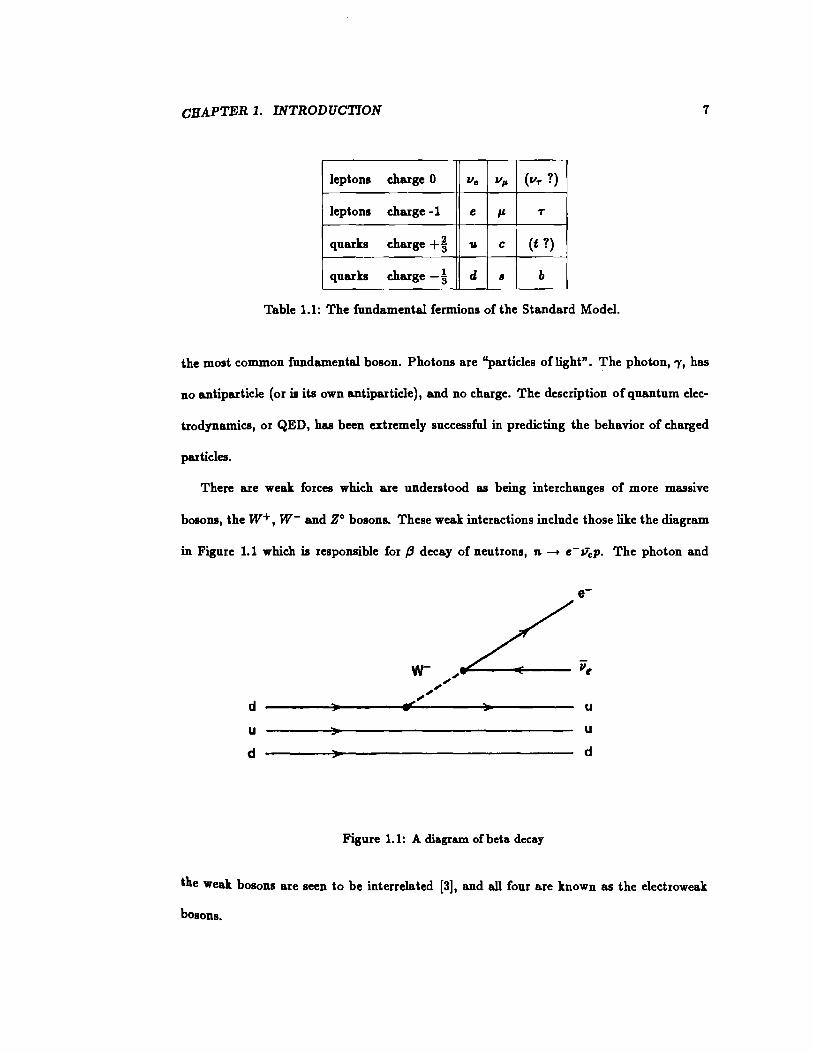
CHAPTER 1. INTRODUCTION 7
leptons charge 0 lie v, (v~ ?)
leptons charge -1 e "' T
quarks charge+~ " c (t ?)
quarks charge-! d • b
Table 1.1: The fundamental fermion& of the Standard Model.
the most common fundamental boson. Photons are "particles oflight". The photon, -y, has
no antiparticle (or is its own antiparticle), and no charge. The description of quantum elec-
trodynamics, or QED, has been extremely successful in predicting the behavior of charged
particles.
There are weak forces which are understood as being interchanges of more massive
bosons, the w+ I w- and zo boson&. These weak interactions include those like the diagram
in Figure 1.1 which is responsible for fJ decay of neutrons, n -+ e-lleP· The photon and
w- ,, ,, "
d ,"
u
u u
d d
Figure 1.1: A diagram ofbeta decay
the weak boson& are seen to be interrelated [3], and all four are known as the electroweak
bosons.
CHAPTER 1. INTRODUCTION 8
Mesons are bound states of a quark and an antiquark. For instance, a B;J meson lS a
bound state of bu, while a B~ meson is bel. Any meson containing only one b or b is termed
a B meson, in general, or also a bottom meson or a b-fl.avored meson. The bb mesons are a
special case briefly mentioned in Section 1.5. The naming of mesons by their quark content
is discussed in detail in Reference (4).
1.3 QCD
In addition to explaining the electroweak forces, the current models attempt to explain the
so called strong forces. These are the forces which are thought to bind quarks together to
form mesons (qq bound states) or baryons (qqq or qqq bound states). It was called the strong
force because the magnitude of this binding energy is higher, and the coupling between the
boson and fermion fields is larger, than for the other known forces.
Due to the rather unique three-fold symmetry needed to describe strong interactions,
this field is called quantum chromodynamics, or QCD, drawing an analogy to color theory,
where red + green + blue = colorless. The QCD model starts with fundamental bosons
called gluons which carry the strong force via "color charge". Each quark can be in any of
three colors, actually called red, green, and blue. Antiquarks come in anticolors, and gluons
carry a color and an anticolor, such as a red-antigreen gluon. Any free particle state must be
colorless, which explains why no free quark or free diquark bound states exist. The strong
coupling, a,, is dependent on the energy of the given interaction. In fact, a, decreases as
the energy increases.
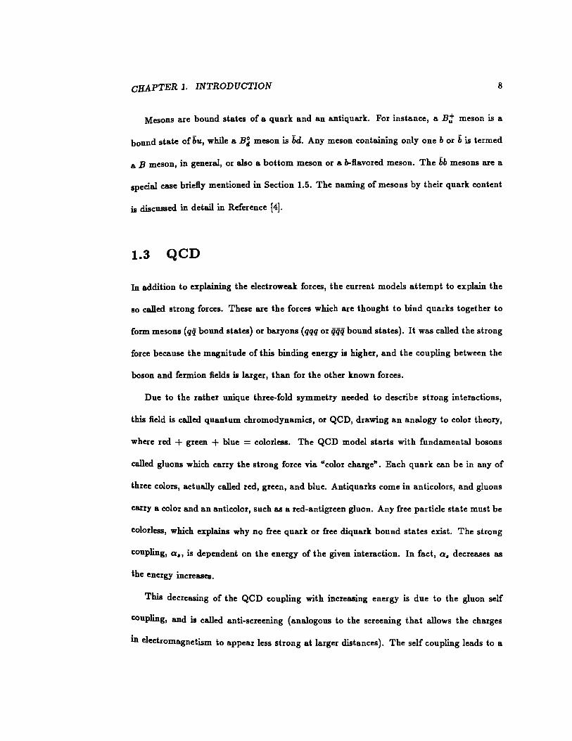
This decreasing of the QCD coupling with increasing energy is due to the gluon self
coupling, and is called anti-screening (analogous to the screening that allows the charges
in electromagnetism to appear less strong at larger distances). The self coupling leads to a
CHAPTER 1. INTRODUCTION 9
0.8
0.6
-. (!)
> ...... -jJ ttl 0.4 ..... (!) 1-1 ..._
1'1)
~
0.2
O.OL-------L-------L-------L-------L-------~~
0 20 40 60 80 100
Energy (arbitrary scale)
Figure 1.2: The energy dependence of a,
CHAPTER 1. INTRODUCTION 10
decreasing dependence of the strong coupling constant a, on the energy of the interaction,
as shown in Figure 1.2. At higher values of energy, there is less coupling strength, while at
lower energies, the coupling is higher. The higher energies probe smaller distances, and the
low coupling region is termed the asymptotic freedom region.
1.4 Interactions
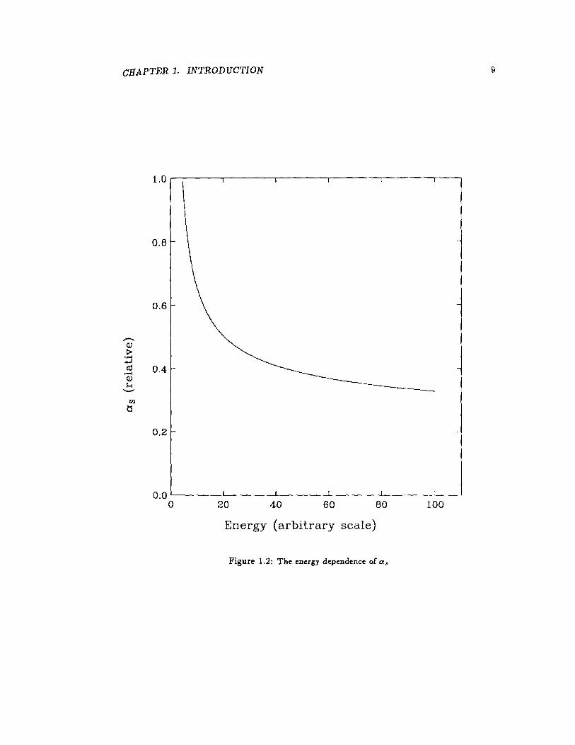
Discussion of the processes in the model will include mention of quantities which depend on
the energies and momenta of the particles involved. It is therefore useful to define some of
these quantities by examination of a simple two-body reaction. Figure 1.3 shows a schematic
1 3
2
Figure 1.3: A two-body reaction
of a two-body process, with particles labelled (1) and (2) coming in, and particles labelled
(3) and (4) :Hying out. The momenta and masses of these particles are labelled p; and m;,
where i is the label number.
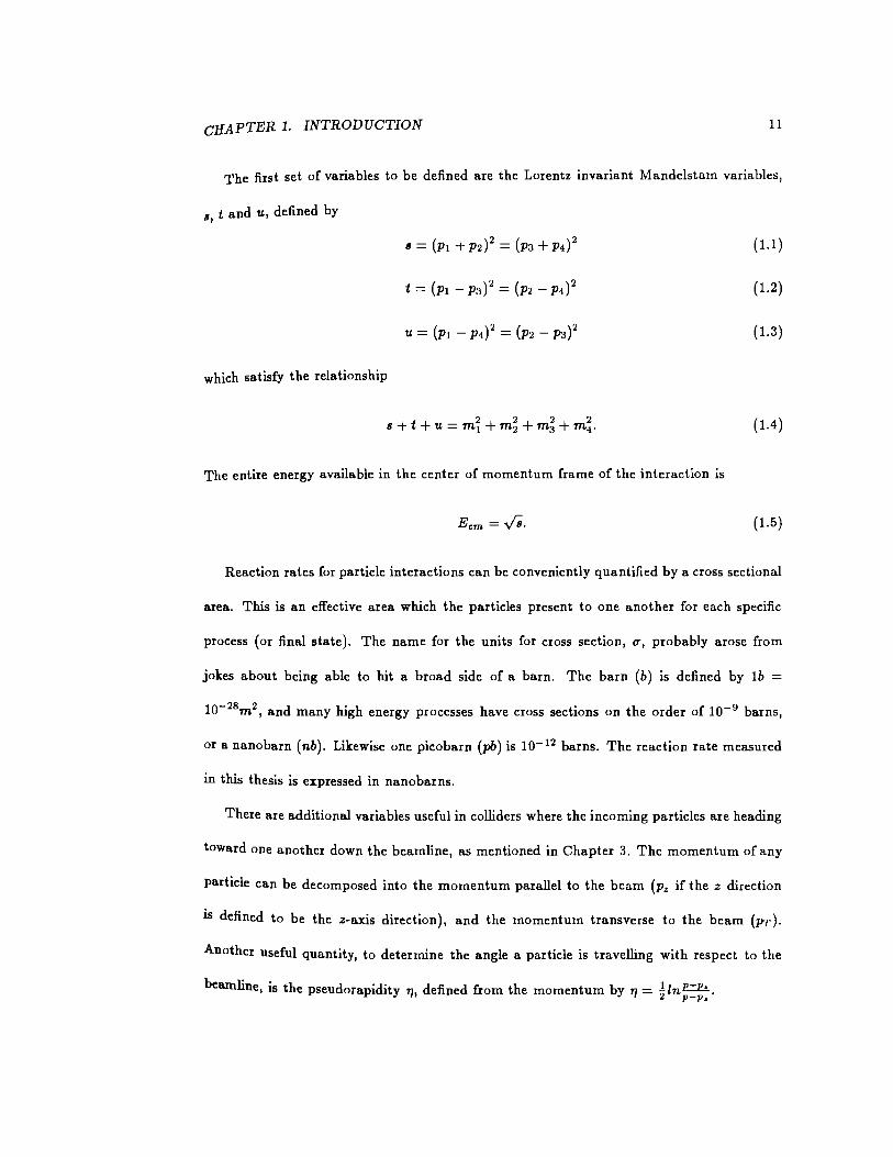
CHAPTER 1. INTRODUCTION 11
The first set of variables to be defined are the Lorentz invariant Mandelstam variables,
61 t and u, defined by
(1.1)
(1.2)
(1.3)
which satisfy the relationship
(1.4)
The entire energy available in the center of momentum frame of the interaction is
Ecm = Vs· (1.5)
Reaction rates for particle interactions can be conveniently quantified by a cross sectional
area. This is an effective area which the particles present to one another for each specific
process (or final state). The name for the units for cross section, u, probably arose from
jokes about being able to hit a broad side of a barn. The barn (b) is defined by 1b = 10-28m 2 , and many high energy processes have cross sections on the order of 10-9 barns,
or a nanobarn (nb). Likewise one picobarn (pb) is I0- 12 barns. The reaction rate measured
in this thesis is expressed in nanobarns.
There are additional variables useful in colliders where the incoming particles are heading
toward one another down the beamline, as mentioned in Chapter 3. The momentum of any
particle can be decomposed into the momentum parallel to the beam (Pz if the z direction
is defined to be the z-axis direction), and the momentum transverse to the beam (PT ).
Another useful quantity, to determine the angle a particle is travelling with respect to the
beamline, is the pseudorapidity 71, defined from the momentum by 11 = -21 lnE..±E..!.. p-p.
CHAPTER 1. INTRODUCTION 12
As mentioned previously, the forces are carried by the exchange of bosons. If the four
momentum of the boson is Q, the quantity Q2 is Lorentz invariant and a useful measure
of the momentum transfer or energy of the interaction. It should be noted that Q2 is not
the mass squared of the boson (unless the boson doesn't interact ever again) and thus the
boson is virtual, or "off the mass shell".
Of course, since protons are made of quarks and gluons, any description of proton inter-
actions with sufficiently high energy to probe this substructure must take this into account.
At the energies discussed in the following chapters, it is necessary to define the Mandelstam
variables for the incoming quarks and gluons for a given partonic interaction, given the
labels 8, i and u. These allow calculation of the partonic cross sections u, that piece of the
total cross section coming from the parton in question. The observable cross section is a
sum of the u from each of the types of partons coming in, as well as integrated over the
initial parton distributions. If z is p(parton)fp(nucleon), the probability distribution that
a parton will have a momentum fraction z is given by F(z, Q2). Note that the distribution
not only depends on the momentum fraction, but also varies with the momentum transfer
probing the interaction Q2 • The total cross section is calculated by
(1.6)
where the sum is over the different types of initial particles a and b. The types of initial
particles are the constituents of the nucleons being collided, like gluons and quarks.
1.5 Quarkonia
With the discovery of the J /..P mesons [5], and the description of the spectroscopy of the
ce system [6], and later the T meson (bb) system [7], the physics of heavy quark - heavy
antiquark bound systems was on its way. These mesons, called quarkonia, or just 'onia'
CHAPTER 1. INTRODUCTION 13
signified by the symbol 0, are bound states of a heavy quark and its anti-quark. Since the
masses of the heavy quarks Q = c or b are very large, they provide a QQ bound-state size
small enough to come near to the asymptotically free regime of the binding a,. This means
the QQ system is probably well described by a perturbative QCD theory. (Mesons with
smaller quark masses are not described well by the first few orders of perturbative QCD).
Comparison of perturbative calculations with experimental observations has yielded infor-
mation of the strong interaction. In fact, the J /1/J and the ,P(2S) were the only charmonia
mesons discovered when the relative masses ofthe other states were predicted [6], especially
the three triplet P states known as the Xc states. The production rate of these Xc states in
the pP interactions is the subject of this thesis.
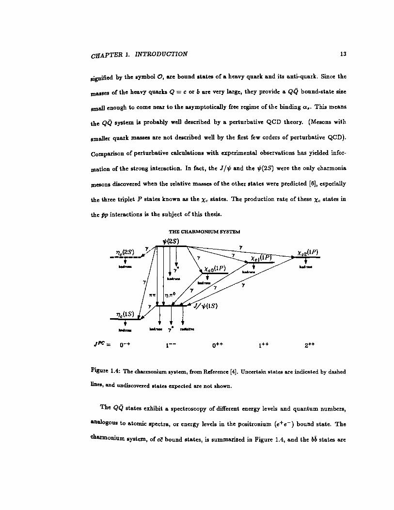
THE CHARMONIUM SYSTEM
1Jc<2s> My !rTTr\::::::::::::::::::::i~-;:-:m"--...!£:~2. ---.--~ -
JPC = o-+ o++ t++
Figure 1.4: The charmonium system, from Reference [4). Uncertain states are indicated by dashed
lines, and undiscovered states expected are not shown.
The QQ states exhibit a spectroscopy of different energy levels and quantum numbers,
analogous to atomic spectra, or energy levels in the positronium (e+e-) bound state. The
c:hannonium system, of cc bound states, is summarized in Figure 1.4, and the bb states are
CHAPTER 1. INTRODUCTION 14
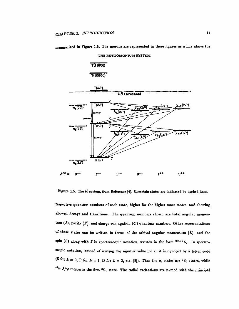
summarised in Figure 1.5. The mesons are represented in these figures as a line above the
JPC = o-+
THE BOTTOMONIUM SYSTEM
T(l1020)
T(10860)
T(4S)
·--
·-·~·-·-·-·-·-·-·-·-·-·-·-·-·-BJJ threshold
o++ t++
Figure 1.5: The bb system, from Reference [4]. Uncertain states are indicated by dashed lines.
respective quantum numbers of each state, higher for the higher mass states, and showing
allowed decays and transitions. The quantum numbers shown are total angular momen-
tum (J), parity (P), and charge conjugation (C) quantum numbers. Other representations
of these states can be written in terms of the orbital angular momentum (L), and the
spin (S) along with J in spectroscopic notation, written in the form 25+1 LJ. In spectro-
scopic notation, instead of writing the number value for L, it is denoted by a letter code
(S for L = 0, P for L = 1, D for L = 2, etc. [8]). Thus the 'lc states are 1So states, while
n,e J /1/J meson is the first 3 S1 state. The radial excitations are named with the principal
CHAPTERl. INTRODUCTION 15
quantum numbers, and since the naming scheme for hadrons [4] includes the rule that 3 S1
states above the J /,Pare named with the greek letter ,P, the next state is labelled the ,P(2S).
The 3 P J states of charmonia are labelled by X.cJ. or X.co,X.cll and X.c2· The bb system has a
similar naming scheme with T denoting the 3 S11 and '1b and X.bJ used for the 1S0 and 3 P J
mesons respectively.
The X.c states can decay electromagnetically into a photon and a J j,P. This is not
the only decay mechanism for the X.c states, but can be significant, (27.3 ± 1.6)% for
X.c1 -+ J f,P-y [4]. The 3S1 states, having the same quantum numbers as the photon, can
decay via the annihilation of the c and c through a virtual photon which can lead to many
final states, including p.+ ,.,.-. Decays into one virtual gluon are forbidden since the mesons
must be color neutral, and 2 gluon decays are accessible only from the states with C = + 1.
Thus the J /,P and ,P(2S) states would decay by three gluons or more. The dilepton final
states can be readily identified (as will be shown in subsequent chapters), so the decays
which will be reconstructed here are X.c -+ J /,P-y, with J /,P-+ p.+ ,.,.-.
1.6 Outline of This Thesis
Some details of the model for charmonia production will be discussed in Chapter 2, listing
the processes to be investigated. The assumptions of this model will be pointed out, and
the processes taken into account will be listed.
The devices for producing and observing these particles will be discussed in Chapter 3,
with emphasis on those parts of the detector which measure muon and photon properties.
Chapter 4 will discuss the collection of the dimuon events with a trigger, and Chapter 5
will delineate the algorithms for reconstruction of the muon and photon candidate objects
in the events gathered. The photon reconstruction is central to the X.c -+ J j,P-y analysis,

CHAPTER 1. INTRODUCTION 16
and will be examined in detail in Chapter 6.
The determination of the overall efficiency of the reconstruction methods used is dis-
cussed in Chapter 7. Details of the final event selection and reconstruction are in Chap-
ter 8. The cross sections are derived from the measurement in Chapter 9, and conclusions
are presented in the final chapter.
Chapter 2
Charmonia Production
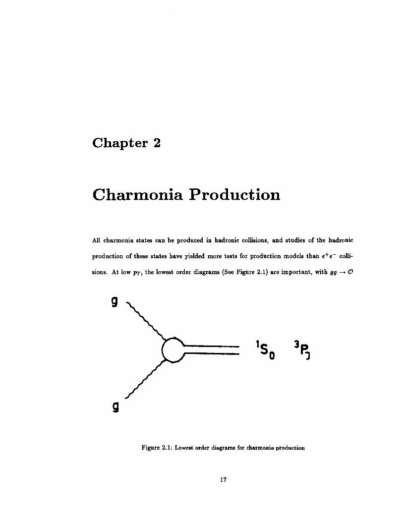
All charmonia states can be produced in hadronic collisions, and studies of the hadronic
production of these states have yielded more tests for production models than e+ e- colli-
sions. At low Pr, the lowest order diagrams (See Figure 2.1) are important, with gg -+ 0
g
g
,s 0
Figure 2.1: Lowest order diagrams for charmonia production
17
CHAPTER 2. CHARMONIA PRODUCTION 18
becoming increasingly dominant (compared to low PT qq- 0) as the (energy) i of there-
action increases [9, 10]. (The J /1/J is not made by gg- J j.,P, because of charge conjugation
invariance (The J /1/J and .,P(2S) are C odd eigenstates), so the statements do not all hold
equally for x and J /1/J).
For high PT charmonia production, higher order diagrams (as in Figure 2.2) become
more significant. In fact, the expectation is that the process gg - Og will constitute the
majority of the production cross section (over the first order processes discussed above) at
collision energies above a few hundred GeV. All these mechanisms are referred to as direct
charmonia production.
Charmonia can also arise from the decays of heavier particles. Decays of b-flavored
mesons into charmonia (via diagrams like that shown in Figure 2.6) have been observed,
and the branching fractions measured in parts per thousand [4]. Because of this the process
gg - bbX - BX - OX (2.1)
must be taken into account. This process, referred to as indirect charmonia production, can
result in high PT charmonia. From the measured cross section, u(b) [11, 12], and branching
fractions of B- Jj.,PX and B- Xc1 X, indirect production ofcharmonia is expected to be
significant.
The J /1/J mesons can be produced in ways other than B decay. Feeddown from other
charmonia states, such as Xc - J /1/Jr is expected to account for much of J j.,P production.
Direct J /1/J production is expected to be small compared to feeddown and B decay produc-
tion at high transverse momenta [9]. In the following sections, direct Xc production and bb
production are outlined.
CHAPTER 2. CHARMONIA PRODUCTION 19
2.1 Direct Charmonia Production
The theoretical model for direct charmonia production discussed here has been outlined in
References [9, 13]. The calculations rest on several assumptions. The first assumption is that
0 are non-relativistic QQ bound states (with Q denoting a heavy quark). Most potential
models for describing charmonia spectroscopy rest on this assumption. The non-relativistic
assumption predicts the proper relative energy levels for the QQ states, but does not work
for quark masses smaller than the charm mass. Secondly, it is supposed that at large PT, 0
production is dominated by order a~ processes, as gg--> QQg, gq--> QQq, and qq--> QQg.
A ser~es of Feynman diagrams can be imagined where the initial light quarks and/or gluons
are constituents of the colliding particles, while the final light quark or gluon result in recoil
jets to offset the transverse momentum of the 0.
Another major axiom of the model is the mechanism by which these diagrams containing
QQ form bound states. It is postulated that the coupling of the bound state 0 to the QQ
pair is directly determined by the appropriate wave function of the state. The wave function
depends on the quantum numbers for spin, angular momentum, and charge conjugation as
well as the color singlet nature of the bound state constructed. This implies that the direct
formation of heavy resonances occurs at short distances, or at least that the QQ eventually
form final states with a probability determined by the quantum wave functions alone. This
assumption of direct formation at short distances leads to spin and color selection rules
which affect the relative weight of contributions from each diagram. This postulate is taken
over an opposing model in which unbound QQ are first produced and then transformed
to 0 by soft processes, leading to a non-perturbative description [14]. Although it has
been attempted [14], production rates would be extremely difficult to calculate for any
non-perturbative model.
CHAPTER 2. CHARMONIA PRODUCTION 20
2.1.1 Matrix Elements
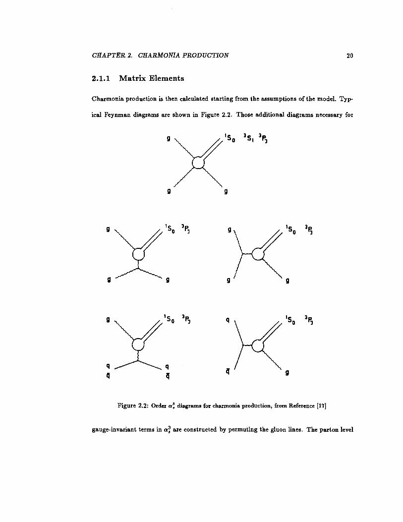
Charmonia production is then calculated starting from the assumptions of the model. Typ-
ical Feynman diagrams are shown in Figure 2.2. Those additional diagrams necessary for
g
g g
g g
g g
Figure 2.2: Order a: diagrams for charmonia production, from Reference [17]
gauge-invariant terms in a~ are constructed by permuting the gluon lines. The parton level
CHAPTER 2. CHARMONIA PRODUCTION 21
cross sections have the form [9, 13]:
d A 3 (1' - a, !( b 2•+1 • 0 A A A 2) dt - 82 w a --+ L, c 1 s, t, u, M (2.2)
where f is a function depending only on selection rules, quantum numbers and the variables
listed, while w depends on the wave function. For P-wave states
(2.3)
where IR~(O)I is the magnitude of the derivative of the radial part of the wave function,
evaluated at the origin and M is the mass of the state.
The full cross section, of course, depends on the parton structure of the colliding particles
and is written
(2.4)
This full cross section calculation has many uncertainties, first among them being uncer-
tainties of the parton structure functions. Second, the strong coupling is calculated by
(2.5)
leaving a choice of scale ambiguity (represented by the choice of Q2 / A2 ). Third, since w
depends on the wave functions, it depends on the potential model used and may not be well
known. Finally, a K factor has been introduced to take into account higher order terms,
and is an additional uncertainty in the calculation. For these reasons, estimations of the
theoretical uncertainties range from ±50% to claims that the predictions should be within
an order of magnitude [9, 13, 15, 16, 17, 18, 19].
2.1.2 Theoretical Uncertainties
The inputs to the theoretical calculation of direct charmonia production include many quan-
tities which are not precisely known. The derivative of the wave function at the origin, the
CHAPTER 2. CHARMONIA PRODUCTION 22
scale chosen to compute a,, and the gluon structure functions will each contribute to the
uncertainty. Furthermore, the K factor, explained as a correction for uncalculated higher
order terms was chosen primarily to fit experimental results at lower energies [9], specifically
J /1/J spectra measured at the ISR [20]. The extrapolation that the cross section at higher
energies will contain the same K factor is another assumption of the model.
The derivative of the wave function at the origin has been examined experimentally by
measuring the hadronic partial width of Xc decays. Under the assumptions of the model,
the value was found from the partial width of the Xc2 state to be IR~(O)j2 = 0.088 ±
0.012 GeV5 [21]. This leads to a value for w = (1.547 ± 0.211) x 10-4 for the xc2 state.
Inputs to most calculations have been in the range 10-4 < w < 2.3 x 10⁻⁴ [21]. The
effect of any change in w would be to scale all cross sections by a constant value. Slopes
of PT distributions and relative rates of each angular momentum state would be relatively
unaffected.
The calculation of a, presents a different problem. Since the cross sections will scale as
a;, small variations in the A 2 choice will be amplified in the cross section measurements.
This would change the calculated cross section for all states and momenta. However, chang-
ing the momentum transfer from Q2 = (p} + m~)/4 to Q2 = m~ (reasonable values due to
the uncertainty of the Q2 of the interaction) would not only change the overall scale, but
would introduce PT dependent effects, which would change the relative production of the Xc
states as well as affecting the calculations of detector acceptance and efficiency.
The gluon structure functions introduce another major theoretical uncertainty. The x
values probed in this analysis ran mostly in the range 0.007 < x < 0.02, while the momentum
transfer was around 9 < Q2 < 200 Ge V2 • The majority of the cross section was at the lower
end of both of these ranges. Monte Carlo studies indicated that most substitutions for
gluon structure functions available would not change the PT spectra dramatically, but would
CHAPTER 2. CHARMONIA PRODUCTION 23
change the overall normalization. Using more recent paramaterizations of the structure
functions [22] would help in predicting the magnitude of the direct cross section expected,
but the acceptance calculations should be relatively unaffected by them [16].
2.2 B Decay to Charmonia
The production rate of b-quarks is thought to be a good place to test QCD. Since the
b quark has a large mass, the momentum transfer of any interaction involving b-quarks
should also be large, on the order of the mass: Q2 :::::: m~. From Equation 2.5 it is clear that
the larger values of Q2 will provide smaller values of a,. In b-quark production theories,
a, is about 0.2. This means that the lower order diagrams will be more important than
higher order diagrams to the full cross section, since with two gluon vertices in a diagram
the contribution is proportional to a:, while three gluon vertices contribute proportional to
a;. Each higher order term should be smaller, and, hopefully, perturbative calculations will
be precise enough to allow a rigorous test of the production theory.
Models of b-hadron production start with parton-parton scattering. The cross section for
b-quark production is calculated. Then, the hadronization ofb-quarks into b-hadrons is mod-
elled. The decomposition of the entire process into hard scattering and soft hadronization
is a key part of the theory explained here.
2.2.1 b Quark Production
The parton level b quark processes are simplest for the order a: diagrams, shown in Fig-
ure 2.3. Diagrams with three gluon vertices, as in Figure 2.4, will contribute to order a~.
Due to interference terms, the order a; calculation must include the four gluon vertex dia-
grams such as in Figure 2.5. These interfere with the 3 gluon vertex diagrams, and are taken
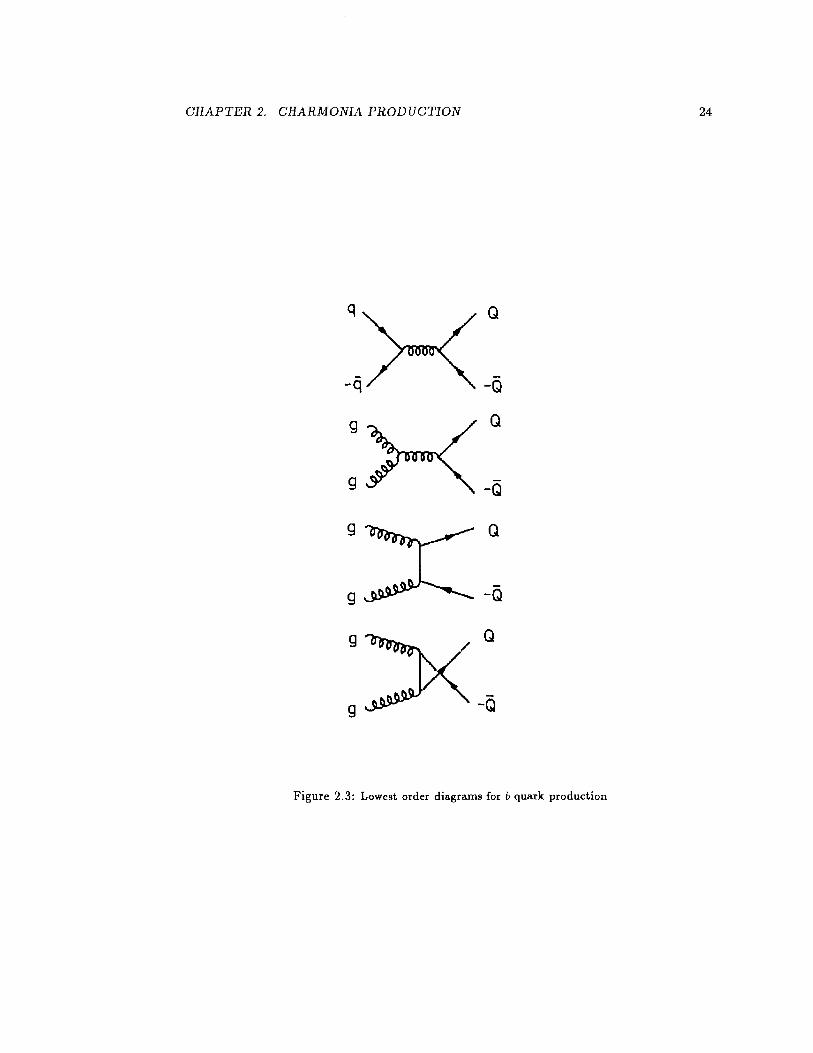
CHAPTER 2. CHARMONIA PRODUCTION
q
-q
g
g
g
g
g
g
Q
-Q
Q
-Q
Q
-Q
Q
-Q
Figure 2.3: Lowest order diagrams for b quark production
24
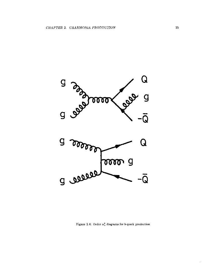
CHAPTER 2. CHARMONIA PRODUCTION 25
g Q
g
g --Q
g Q
g -g -Q
Figure 2 .4: Order o:~ diagrams for b-quark production
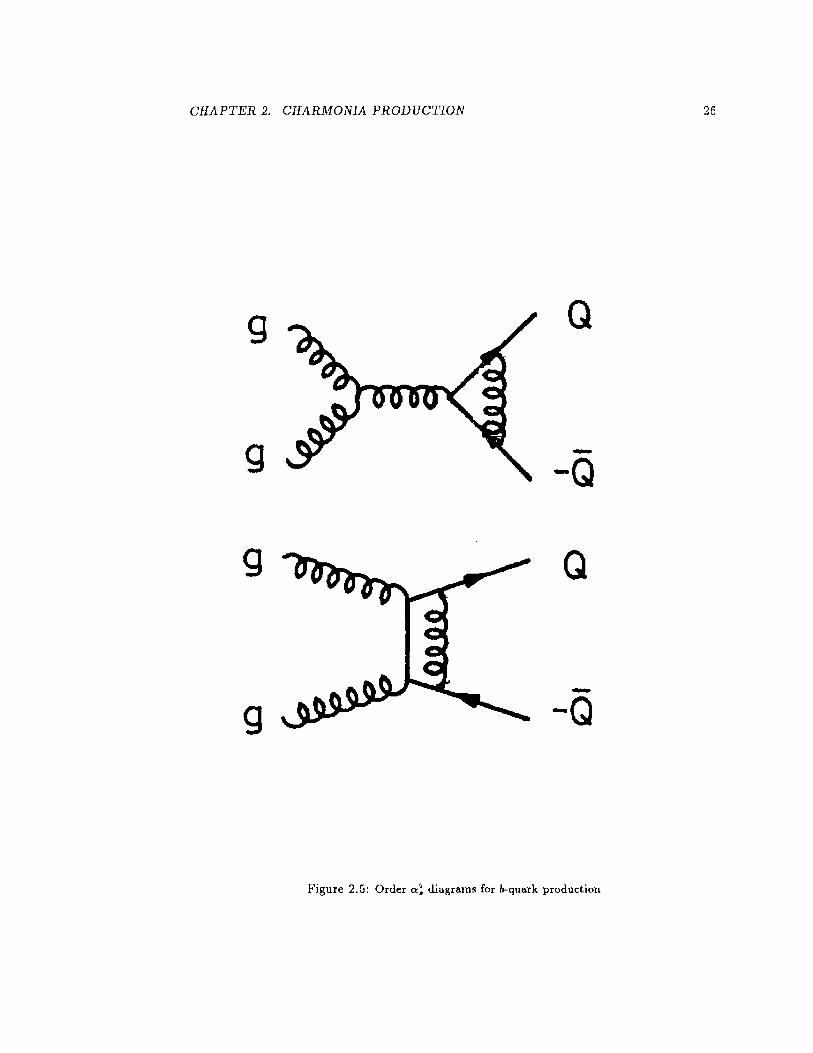
CHAPTER 2. CHARMONIA PRODUCTION 26
g Q
g --Q
g Q
-g -Q
Figure 2.5: Order o:! diagrams for b-quark production
CHAPTER 2. CHARMONIA PRODUCTION 27
into account in the a: calculation performed by Nason, Dawson, and Ellis (NDE) [23]. The
NDE matrix elements were used in the b Monte Carlos for this analysis.
The details of the NDE calculation will not be described here but it should be noted that
the same types of uncertainties arise in this QCD calculation as in the direct Xc production
theory. For instance, the exact Q2 to use is unclear, and the same range of choices is
available, for instance Q2 = pf + m~ or Q2 = 4m~. The gluon structure function drives the
magnitude of the cross section as well. While the larger mass of the b quark should decrease
the importance of higher order terms, the value for the mass has an additional uncertainty.
For instance, theoretical inputs to models usually place the b quark mass between 4.5 and
2.2.2 b Fragmentation
A simulation of b-quark fragmentation relied on the Peterson fragmentation model [24]. The
b-hadron was assigned a transverse momentum that was some fraction of the initial quark
transverse momentum. If z is the ratio of the final b-hadron PT and the initial b-quark PI'•
the distribution of the number of B-mesons (N) versus z follows
dN z(1- z)~ - oc ---'-----,-----'---,-,,..,-dz [EpZ + (1- z)2J2 (2.6)
with the Peterson parameter Ep an input to the theory. Experimental results indicate Ep = 0.006 ± 0.002 [25]
When the b-quark pulls an antiquark out ofthe vacuum to become a meson, the antiquark
can be any flavor, although the higher mass flavors are much less likely. In fact, the c and
b contributions out of the vacuum can be neglected, and the u and d are about equal. This
leads to the definition of >.,, which is the ratio of s quarks with respect to the two light
quarks pulled out of the vacuum, i.e. u:d:s = 1:1:>.,. Experimentally, >., has been measured
CHAPTER 2. CHARMONIA PRODUCTION 28
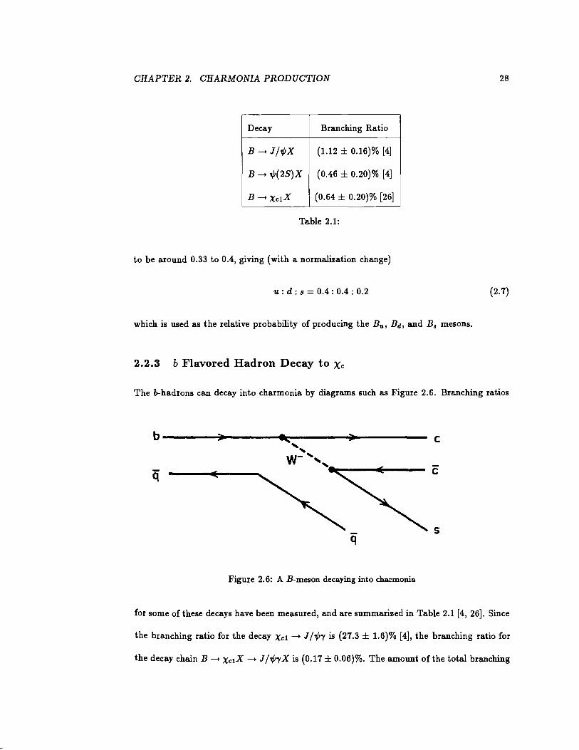
Decay Branching Ratio
B--+ JNX (1.12 ± 0.16)% [4]
B--+ .,P(2S)X (0.46 ± 0.20)% [4]
B--+ XclX (0.64 ± 0.20)% [26]
Table 2.1:
to be around 0.33 to 0.4, giving (with a normalization change)
1£ : d : s = 0.4: 0.4 : 0.2 (2.7)
which is used as the relative probability of producing the Bu, Bd, and B. mesons.
2.2.3 b Flavored Hadron Decay to Xc
The b-hadrons can decay into charmonia by diagrams such as Figure 2.6. Branching ratios
b c ,, w-' ,, c q
5 q
Figure 2. 6: A B-meson decaying into charmonia
for some ofthese decays have been measured, and are summarized in Table 2.1 [4, 26]. Since
the branching ratio for the decay Xcl --+ J /1/Jr is (27.3 ± 1.6)% [4], the branching ratio for
the decay chain B--+ Xc1X--+ Jf.,PrX is (0.17 ± 0.06)%. The amount ofthe total branching
CHAPTER 2. CHARMONIA PRODUCTION 29
fraction to J j.,P due to decays through Xc1 is then
Br(B-+ XclX-+ J N'YX) rx = Br(B -+ J NX) = 0.15 ± 0.05. (2.8)
This result is used in Chapter 9 to relate the measured Xc and J /1/J cross sections to the
direct and B-decay charmonia cross sections.
2.3 Inclusive Charmonia Production
An understanding of the total charmonia cross section can only come from understanding
each mechanism for charmonia production. Measurements of the inclusive Xc cross section,
presented in this thesis, along with measurements of the inclusive J j.,P cross section, yield
information on each of the major modes of charmonium production. This is done in detail
in Section 9.2.
Chapter 3
The Experimental Environment
The Collider Detector at Fermilab (CDF) was a general purpose particle detector located
at the BO interaction region in the Tevatron, at Fermi National Accelerator Laboratory.
During the time the data was taken for this analysis, the Tevatron was the highest energy
accelerator in the world, providing proton-antiproton collisions at a center of mass energy
of 1.8 TeV. Such high energy collisions have provided insight into many physical processes.
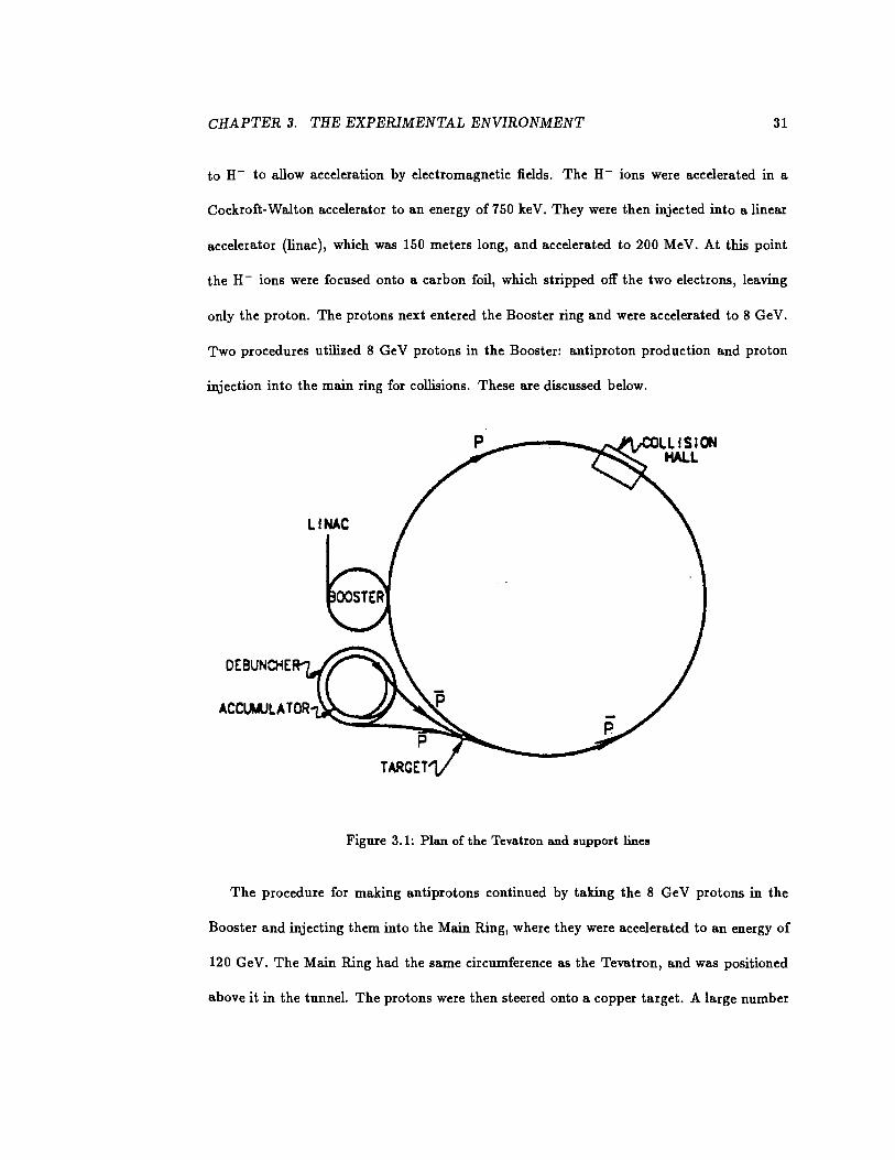
3.1 The Tevatron
The Tevatron was a superconducting synchotron built for the purpose of colliding protons
against antiprotons at high energy to probe subatomic behavior. Superconducting magnets
produced magnetic fields which curved the charged particles in a four mile circle through
a vacuum tube in an underground tunnel at Fermilab. The Tevatron layout is shown in
Figure 3.1, including the supporting lines. Fixed target lines are not shown.
The process of colliding protons and antiprotons starts with hydrogen gas, which is
molecules of H2 , or two H atoms, each with a proton and electron. The gas was ionized
30
CHAPTER 3. THE EXPERIMENTAL ENVIRONMENT 31
to H- to allow acceleration by electromagnetic fields. The H- ions were accelerated in a
Cockroft-Walton accelerator to an energy of 750 ke V. They were then injected into a linear
accelerator (linac), which was 150 meters long, and accelerated to 200 MeV. At this point
the H- ions were focused onto a carbon foil, which stripped off the two electrons, leaving
only the proton. The protons next entered the Booster ring and were accelerated to 8 Ge V.
Two procedures utilized 8 GeV protons in the Booster: antiproton production and proton
injection into the main ring for collisions. These are discussed below.
OEBUNCHE
Figure 3.1: Plan of the Tevatron and support lines
The procedure for making antiprotons continued by taking the 8 Ge V protons in the
Booster and injecting them into the Main Ring, where they were accelerated to an energy of
120 GeV. The Main Ring had the same circumference as the Tevatron, and was positioned
above it in the tunnel. The protons were then steered onto a copper target. A large number
CHAPTER 3. THE EXPERIMENTAL ENVIRONMENT 32
of different particles were produced in the resulting collision, some of which were antiprotons.
Those antiprotons with an energy near 8 GeV were collected, sent to the Debuncher, and
cooled. The antiprotons were then stacked in the antiproton Accumulator ring, until about
27 x 1010 were stored.
To prepare for colliding operation, the cycle was as follows. Protons were injected from
the Booster into the Main Ring, and accelerated to the energy of 150 GeV. In the main ring,
the protons were forced into one bunch consisting of about 7 x 10¹⁰ protons. This proton
bunch was injected into the Tevatron, circulating clockwise and waiting for the antiprotons.
During the 1988-89 run, the Tevatron ran in six bunch mode, so this injection procedure
was repeated six times, resulting in six bunches around the ring.
Antiprotons from the Accumulator were than directed to the Main Ring, and, like the
protons, were accelerated to an energy of 150 GeV. Since opposite charges curve in opposite
directions in a magnetic field, the antiprotons were circulated counterclockwise, the opposite
direction to that of the protons. At last the antiprotons were injected into the Tevatron to
join the protons. Six bunches of antiprotons were injected, spaced about the ring.
At this point, diffuse bunches of protons and antiprotons were counter-rotating in the
Tevatron at 150 GeV. The magnetic fields of the Tevatron magnets were increased as the
particles were accelerated to the final beam energy of 900 GeV. The density of the beams
was increased by a series of quadrupole focusing magnets, squeezing the particles together.
This focusing constricted the beam spot size to less than 100 p,m in diameter, ensuring an
almost 100 % probability of interaction for each bunch crossing.
Bunches crossed at the BO interaction point once every 3.5 p,s. The counter-rotating
beams could be sustained for over 20 hours until the luminosity would drop off, and a new
store was prepared with the same cycle of events.
CHAPTER 3. THE EXPERIMENTAL ENVIRONMENT 33
3.2 CDF
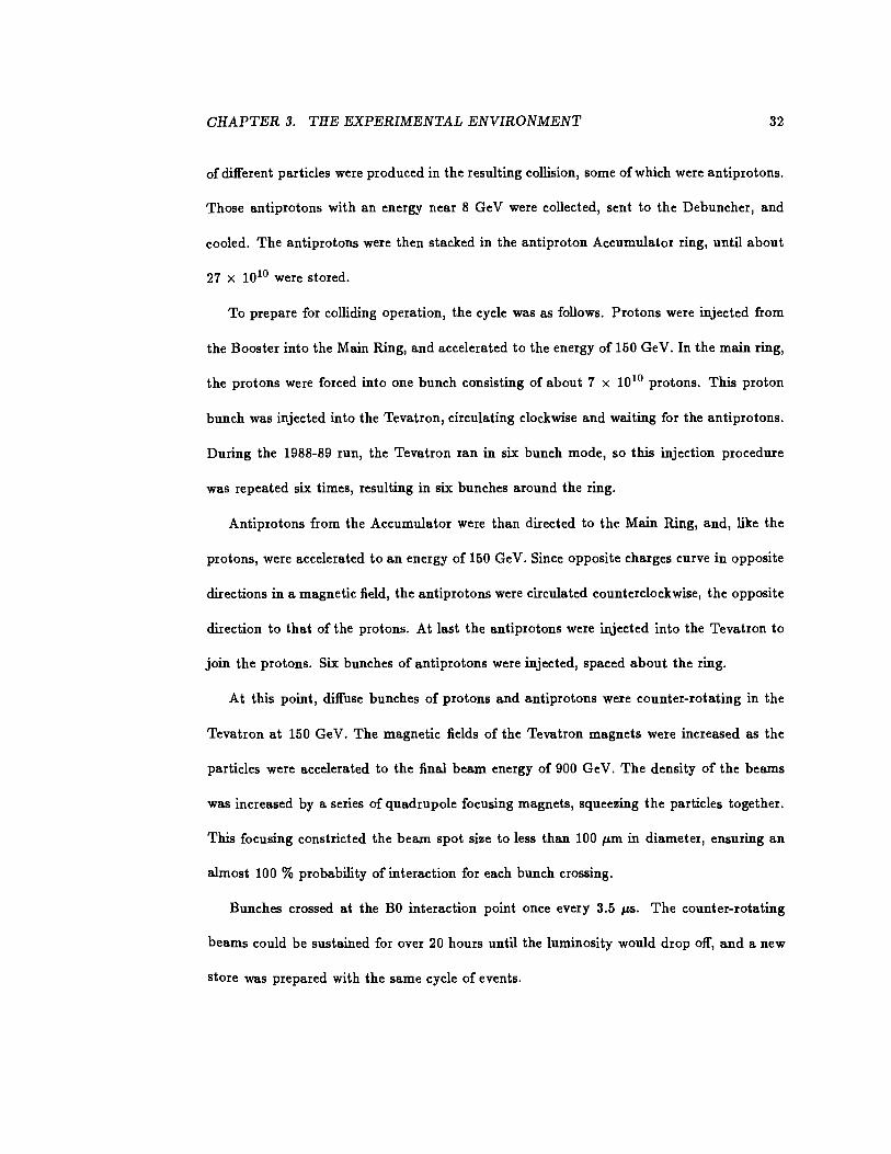
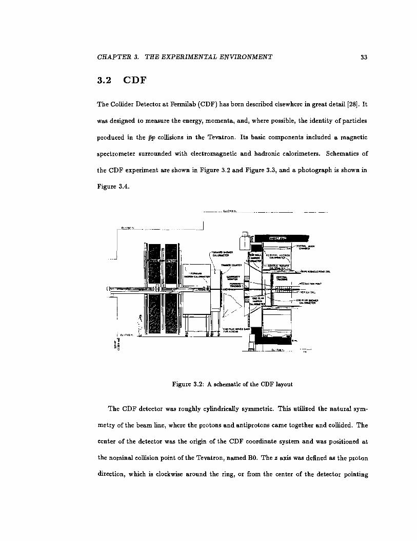
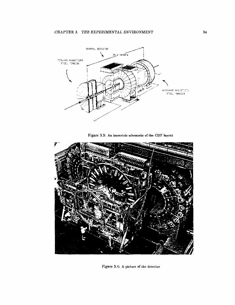
The Collider Detector at Fermilab (CDF) has been described elsewhere in great detail [28]. It
was designed to measure the energy, momenta, and, where possible, the identity of particles
produced in the fp collisions in the Tevatron. Its basic components included a magnetic
spectrometer surrounded with electromagnetic and hadronic calorimeters. Schematics of
the CDF experiment are shown in Figure 3.2 and Figure 3.3, and a photograph is shown in
Figure 3.4.
~r·-" ---- ________ r-.u.cli>JL ______ ----
-~-· ...
Figure 3.2: A schematic of the CDF layout
The CDF detector was roughly cylindrically symmetric. This utilized the natural sym-
metry of the beam line, where the protons and antiprotons came together and collided. The
center of the detector was the origin of the CDF coordinate system and was positioned at
the nominal collision point of the Tevatron, named BO. The z axis was defined as the proton
direction, which is clockwise around the ring, or from the center of the detector pointing
CHAPTER 3. THE EXPERIMENTAL ENVIRONMENT
~:~~!~J ~LGNE~IZED
~-:::::_ -2ri0!8S
CENTRA~ DETECTOR
Figure 3.3: An isometric schematic of the CDF layout
Figure 3.4: A picture of the detector
34
CHAPTER 3. THE EXPERIMENTAL ENVIRONMENT 35
east. The a: axis lay on the ring plane, and pointed out. The y axis pointed up, perpendicu-
lar to the ring plane. The angle about the z axis, ¢, was 0 on the positive x axis. The polar
angle, (), was 0 on the positive z axis. The pseudorapidity, 71, was defined by 71 = -ln tan~
The 'central region' was the term given to the region -1 < 71 < 1 or about 40° < () < 140°.
The detector in the central region included tracking, calorimeters, and muon identification.
The forward region included calorimeters and muon toroids.
The beampipe was a low mass vacuum chamber of 500 micron thick beryllium with an
outer radius of 5.08 em. It is part of the vacuum system of the Tevatron, and is along the
beam axis through the center ofthe detector. The pressure maintained in the beampipe was
less than :::::: 10-8 torr absolute, so the beam-gas interaction rate was very low at reasonable
luminosities. The low mass requirement was to minimize multiple Coulomb scattering before
particles entered the detector and to reduce charged particles which resulted from photons
converting to e+ e- pairs.
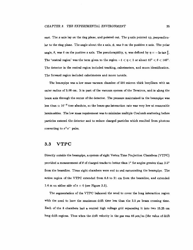
3.3 VTPC
Directly outside the beampipe, a system of eight Vertex Time Projection Chambers (VTPC)
provided a measurement of() of charged tracks to better than 1° for angles greater than 3.5°
from the beamline. These eight chambers were end to end surrounding the beampipe. The
active region of the VTPC extended from 6.8 to 21 em from the beamline, and extended
1.4 m on either side of z = 0 (see Figure 3.5).
The segmentation of the VTPC balanced the need to cover the long interaction region
with the need to have the maximum drift time less than the 3.5 IJ.S beam crossing time.
Each of the 8 chambers had a central high voltage grid separating it into two 15.25 em
long drift regions. Thus when the drift velocity in the gas was 46 IJ.m/ns (the value of drift
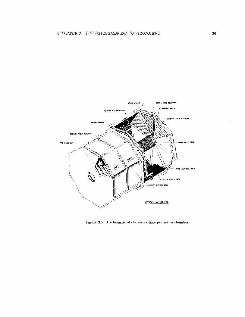
CHAPTER 3. THE EXPERIMENTAL ENVIRONMENT 36
(!tfTEA H.'li QIUD-----.
\ FIAOI.AL BOAMJo~
C.M BON ... Ill OCTCO ON -
I
I .\\
VTPC. MODULES
Figure 3.5: A schematic of the vertex time projection chamber
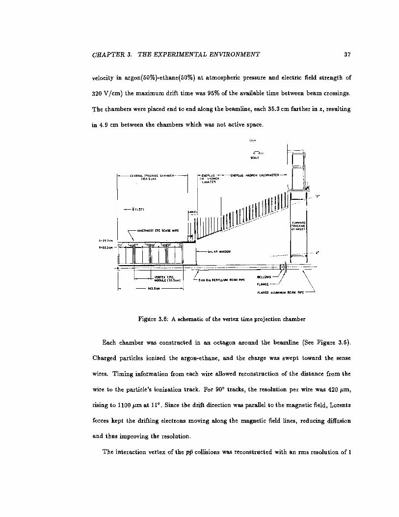
CHAPTER 3. THE EXPERIMENTAL ENVIRONMENT 37
velocity in argon(50%)-ethane(50%) at atmospheric pressure and electric field strength of
320 V /em) the maximum drift time was 95% of the available time between beam crossings.
The chambers were placed end to end along the beamline, each 35.3 em farther in z, resulting
in 4.9 em between the chambers which was not active space.
t----- 14l.'"" ----!
OOL D ""'
SCALE
~~· \ FLMED .&LUMlMJM IEAW PIPE
Figure 3.6: A schematic of the vertex time projection chamber
Each chamber was constructed in an octagon around the beamline (See Figure 3.6).
Charged particles ionized the argon-ethane, and the charge was swept toward the sense
wires. Timing information from each wire allowed reconstruction of the distance from the
wire to the particle's ionization track. For 90° tracks, the resolution per wire was 420 p,m,
rising to 1100 p,m at 11°. Since the drift direction was parallel to the magnetic field, Lorentz
forces kept the drifting electrons moving along the magnetic field lines, reducing diffusion
and thus improving the resolution.
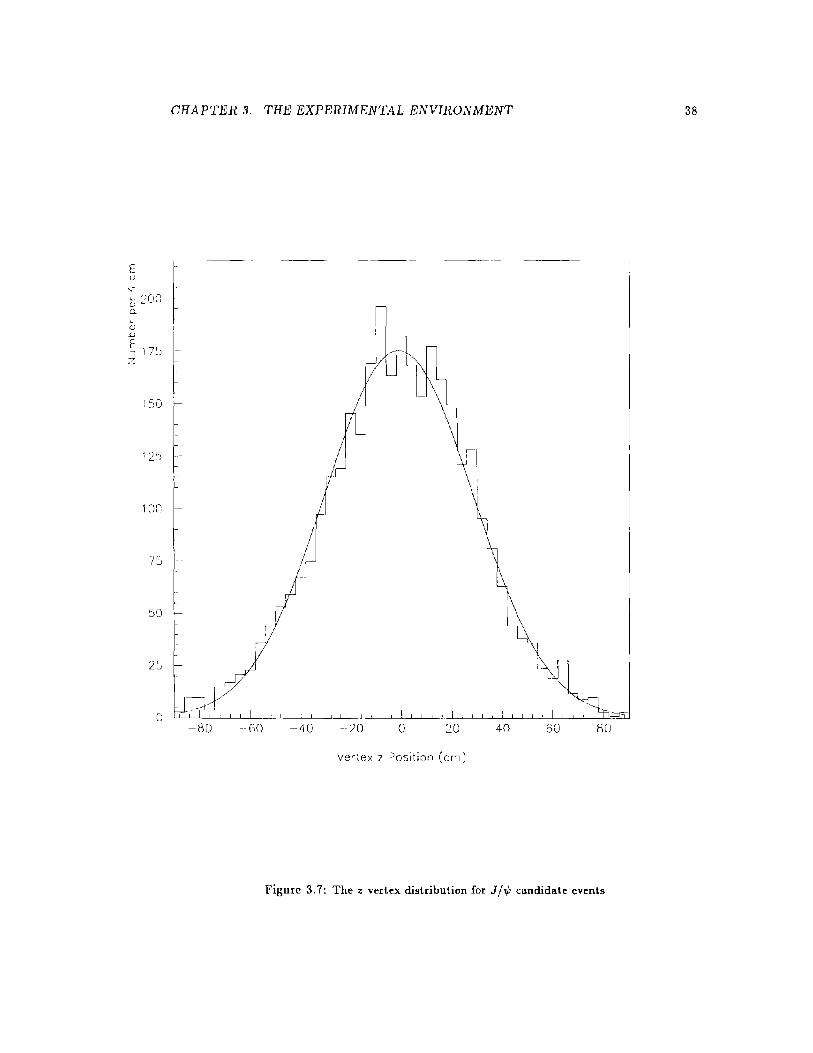
The interaction vertex of the pP collisions was reconstructed with an rms resolution of 1
CHAPTER 3. THE EXPERIMENTAL ENVIRONMENT 38
E r u
" ~- '~II'' c.:..:__ ._..u G. c 0 D
l HI~ I E 1 "7C =' J .J z
:so
f \ 1:25 I I
r
I
10CJ
7S
jQ 1\ '\J~
l!!llll,,,~
2'::l
~ y -- / ~-t:J o' 1 1 1 1 1 1 I I I I I I I I I I I I I I I I I I l ' I
-80 -GO -20 0 20 40 60 80
Ver~ex z !'osition (ern)
Figure 3. 7: The z vertex distribution for J /'1/J candidate events
CHAPTER 3. THE EXPERIMENTAL ENVIRONMENT 39
mm in the z direction. This vertex was used as the origin in computing the transverse energy
( ET = E sin 0) deposited in each calorimeter cell. The distribution in z of reconstructed
vertices in events with two muons is shown in Figure 3.7 and is well described as a Gaussian
of mean -1 em and width 30 em. This spread of vertices reflects the convolution of the
proton and antiproton bunches in the collider. Thus the vertices were within the 2.8 m long
active region of the VTPC.
3.4 CTC
The Central Tracking Chamber (CTC) measured the trajectories of charged particles that
traversed the active CTC volume. These trajectories were important for three reasons. The
first was the precise determination of particle momentum. The second was the identification
of leptons. The third was identification of secondary vertices from long lived particle decays.
Momentum determination required knowledge of the track parameters and the magnetic
field. In the presence of the magnetic field, charged particles travelled a helical path. The
radius, R, of the helix is related to the momentum of the particle, p, by the rdation
IPI cos>.= cqiBIR (3.1)
where >. is the pitch angle of the helix, q the charge of the particle, B is the magnetic field,
and c is the speed of light. Since the magnetic field was aligned with the beamline, IPI cos>.
was just PT, the transverse momentum of the particle.
Lepton identification relied on matching the CTC track with tracks or clusters in other
parts of the detector. Electrons were identified by matching tracks to energy deposition in
the electromagnetic calorimeters. Muons were identified by matching CTC tracks to tracks
in the muon chambers. These detectors will be discussed in detail in a later section.

CHAPTER 3. THE EXPERIMENTAL ENVIRONMENT 39
mm in the z direction. This vertex was used as the origin in computing the transverse energy
(ET = E sin 9) deposited in each calorimeter cell. The distribution in z of reconstructed
vertices in events with two muons is shown in Figure 3. 7 and is well described as a Gaussian
of mean -1 em and width 30 em. This spread of vertices reflects the convolution of the
proton and antiproton bunches in the collider. Thus the vertices were within the 2.8 m long
active region of the VTPC.
3.4 CTC
The Central Tracking Chamber ( CTC) measured the trajectories of charged particles that
traversed the active CTC volume. These trajectories were important for three reasons. The
first was the precise determination of particle momentum. The second was the identification
ofleptons. The third was identification of secondary vertices from long lived particle decays.
Momentum determination required knowledge of the track parameters and the magnetic
field. In the presence of the magnetic field, charged particles travelled a helical path. The
radius, R, of the helix is related to the momentum of the particle, p, by the relation
IPI cos~= cqiBIR (3.1)
where ~ is the pitch angle of the helix, q the charge of the particle, B is the magnetic field,
and c is the speed of light. Since the magnetic field was aligned with the beamline, IPI cos~
was just PT, the transverse momentum of the particle.
Lepton identification relied on matching the CTC track with tracks or clusters in other
parts of the detector. Electrons were identified by matching tracks to energy deposition in
the electromagnetic calorimeters. Muons were identified by matching CTC tracks to tracks
in the muon chambers. These detectors will be discussed in detail in a later section.
CHAPTER 3. THE EXPERIMENTAL ENVIRONMENT 40
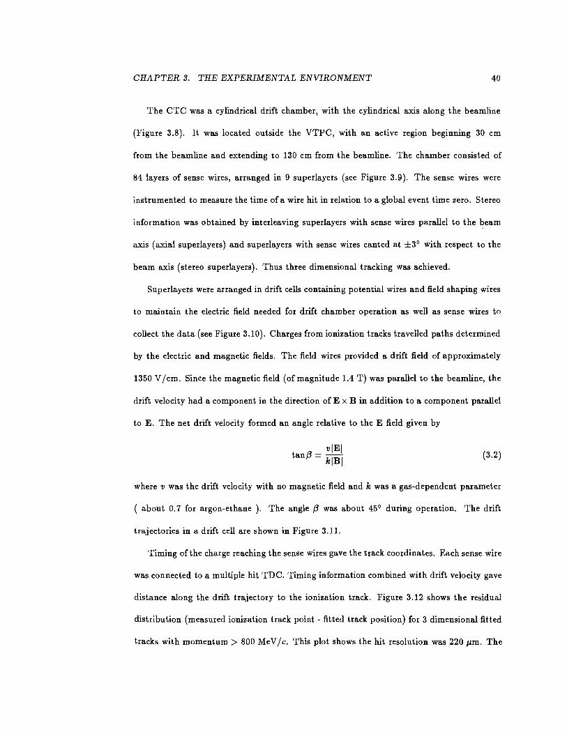
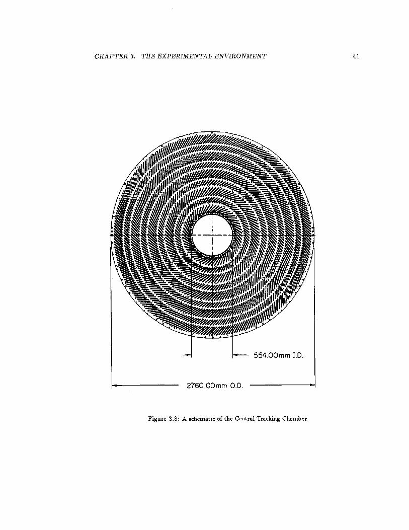
The CTC was a cylindrical drift chamber, with the cylindrical axis along the beamline
(Figure 3.8). It was located outside the VTPC, with an active region beginning 30 em
from the beamline and extending to 130 em from the beamline. The chamber consisted of
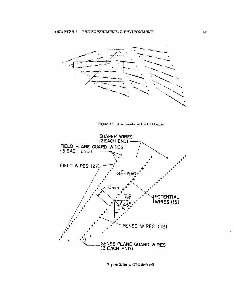
84 layers of sense wires, arranged in 9 superlayers (see Figure 3.9). The sense wires were
instrumented to measure the time of a wire hit in relation to a global event time zero. Stereo
information was obtained by interleaving superlayers with sense wires parallel to the beam
axis (axial superlayers) and superlayers with sense wires canted at ±3° with respect to the
beam axis (stereo superlayers). Thus three dimensional tracking was achieved.
Superlayers were arranged in drift cells containing potential wires and field shaping wires
to maintain the electric field needed for drift chamber operation as well as sense wires to
collect the data (see Figure 3.10). Charges from ionization tracks travelled paths determined
by the electric and magnetic fields. The field wires provided a drift field of approximately
1350 VI em. Since the magnetic field (of magnitude 1.4 T) was parallel to the beamline, the
drift velocity had a component in the direction of Ex B in addition to a component parallel
to E. The net drift velocity formed an angle relative to the E field given by
viE I tan/3 = kiBI (3.2)
where v was the drift velocity with no magnetic field and k was a gas-dependent parameter
( about 0. 7 for argon-ethane ). The angle t3 was about 45° during operation. The drift
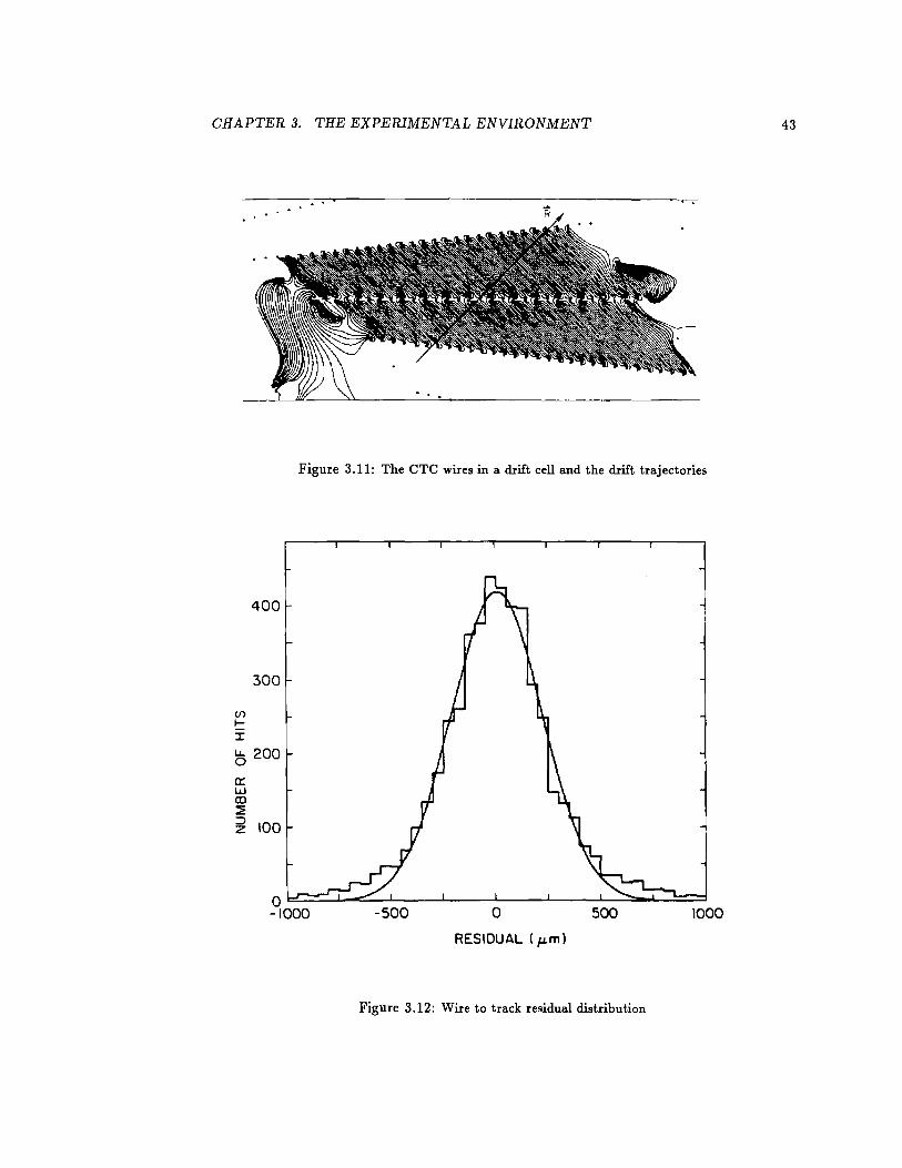
trajectories in a drift cell are shown in Figure 3.11.
Timing of the charge reaching the sense wires gave the track coordinates. Each sense wire
was connected to a multiple hit TDC. Timing information combined with drift velocity gave
distance along the drift trajectory to the ionization track. Figure 3.12 shows the residual
distribution (measured ionization track point - fitted track position) for 3 dimensional fitted
tracks with momentum > 800 MeV I c. This plot shows the hit resolution was 220 /LID. The
CHAPTER 3. THE EXPERIMENTAL ENVIRONMENT 41
554.00mm I.D.
2760.00mm 0.0.
Figure 3.8: A schematic of the Central Tracking Chamber
CHAPTER 3. THE EXPERIMENTAL ENVIRONMENT
•
.~~·· .~ .... ........... . ............ ,.. ••••••••• R • • .................. . ... .. ................ ······t• ..... . ....... . ... ..... . ............ . ····· ........... . •.•. .•• ,---.,..,.,,................:..:..:..:..______-';>L---.._,.............. ·:········· ·•••• . .. ... ····· ................ .... ··········· . ............ ······ ········ .................... . ..... ······ ............. . ....... .. ............. . ............... . .._ . ······ ... ············· ...
L-------r~....,..,.=-----' ······ ·•···· ·····
................ . ................ . . . ······· . ······ . .. ······· . ·············· .......... .... . .. . ··········· ... .....,. ..... ·· .... .. ......... . . .. ······· .. .. . ....... ... .. .. , ····· ....... ·· .. . ...... . .
Figure 3.9: A schematic of the CTC wires
SHAPER WIRES (2 EACH END) --
.. .. .. . .. .. ...
FIELD PLANE GUARD WIRES (3EACH END)~
• • • • • • •
FIELD WIRES (27) • • + ••
• •
•
. • •
. ....... . . • 08=15kG+ •• • • •
• • + •• • • + • :· ,( !Omm + • ••• ....... ~'>j0{....... :i~~~~~~~~
• • E •• • + ... • • r • •
+·~ • • • SENSE WIRES ( 12) + • • • •
'~ • SENSE PLANE GUARD WIRES ~(3 EACH END)
Figure 3.10: A CTC drift cell
42
CHAPTER 3. THE EXPERIMENTAL ENVIRONMENT
Figure 3.11: The CTC wires in a drift cell and the drift trajectories
U') I-I
400
300
~ 200 0:: w co ~
~ 100
o~~~~~~----~--~~--~----~~~._~-=
-1000 -500 0 500 1000
RESIDUAL ( fLm)
Figure 3.12: Wire to track residual distribution
43
CHAPTER 3. THE EXPERIMENTAL ENVIRONMENT 44
resolution of a stereo wire in the longitudinal (z) coordinate would be (220 JLm)/(sin 3°) = 4.2 mm.
Since multiple coulomb scattering and energy loss in matter before the particles have
been measured can affect the resolution, it was important to minimize the amount of material
in front of the tracking chambers. In addition, the great number of photons produced per
event would interact with matter and pair produce e+ e-, adding tracks not produced in the
initial event. For these reasons, the detector was constructed with low mass materials, to
minimize the number of radiation lengths traversed by particles before they encountered the
CTC active volume. About 3% of a radiation length was traversed by tracks perpendicular
to the beam line before reaching the CTC active volume. About 0.5% of a radiation length
was from the beampipe, while the VTPC contributed 1.5% of a radiation length. The
remainder was due to the CTC inner wall. At angles closer to the beam pipe, more material
was traversed, scaling as 1/ sin ( 6) in the central region until the end of the CTC was reached.
3.5 Solenoid
The magnetic field was produced by a 3 m diameter 5 m long superconducting solenoid
coil [29] (visible in Figure 3.2). The coil consisted of 1164 turns ofNbTi/Cu superconducting
metal alloy, stabilized with aluminum. The overall thickness of the solenoid, support and
cooling material was 0.85 radiation lengths.
The solenoid provided a uniform 1.46 T magnetic field oriented along the beam direction.
The field was produced by a current of 4659 A flowing in the superconducting material. A
steel flux return yoke encased the entire detector, forming a large box 9.4 m high by 7.6 m
wide by 7.3 m long. This yoke, in addition to its function as a magnetic flux return path,
supported the solenoid and end plug calorimeters.
CHAPTER 3. THE EXPERIMENTAL ENVIRONMENT 45
3.6 Calorimeters
In addition to the magnetic spectrometry provided by the tracking systems, CDF included
electromagnetic and hadronic calorimeters. The goals of the CDF calorimeters were com-
plementary to the tracking. The calorimeters, constructed in a projective tower geometry,
measured the energy of both charged and neutral particles in a tower, whereas the tracking
measured momenta of individual charged particles. Projective tower geometry means that
the calorimeter was separated into 11- ¢ sections or "towers" which pointed back radially
to the interaction region at z = 0. The calorimeters were helpful in particle identification,
most especially electrons and photons, and gave information to help identify muons and
select hadronic jets. The calorimeters were segmented longitudinally into electromagnetic
and hadronic sections.
3.6.1 Electromagnetic Calorimeters
The electromagnetic calorimeters measured the energy of incident electrons, positrons, and
photons by sampling the energy deposited in an electromagnetic cascade. They also aided
in the identification of e± and 'Y by matching clusters of energy with tracks from the CTC.
The Central Electromagnetic Calorimeter ( CEM) surrounded the solenoid, covering the
region 1111 < 1. The CEM consisted of sheets of lead radiator interleaved with sheets of
scintillating polystyrene (Figure 3.13). Particles interacted with the lead by bremsstrahlung
and pair production to produce an e± and 1 cascade. The charged particles then passed
through the scintillator, which produced light when traversed by charged particles. This
light was transmitted by waveshifting plastic to light guides leading to phototubes which
measured the intensity.
Since most particles of interest would originate near the center of the detector, the
CHAPTER 3. THE EXPERIMENTAL ENVIRONMENT
LEAD SCINTILLATOR SANDWICH-
STRIP CHAMBER
z
y
111----lf----c:;,- Ll GHT
Figure 3.13: A schematic of the CEM
GUIDES
WAVE SHIFTER SHEETS
46
CHAPTER 3. THE EXPERIMENTAL ENVIRONMENT 47
calorimeters were arranged in a projective tower geometry. These towers surrounded the
solenoid, and were ganged into wedges. Figure 3.13 shows one wedge. There were a total
of 48 wedges, arrayed in two concentric cylinders of 24 wedges each. These cylinders were
end to end on the z axis, and centered at the CDF origin. Each wedge was comprised of
10 projective towers pointing to the collision point. The segmentation of each tower was
flTJ x .6.¢ = .09 X 15°. The towers covered from TJ=O to TJ = ± 1.1, the sign being determined
by which cylinder the wedge was in.
The construction of the CEM is shown in Figure 3.14. There were 31 lead layers, each
0.32 em thick. After each lead layer, there was 0.5 em of SCSN-38 polystyrene scintillator
[30]. All layers of Pb and scintillator added up to the 18 radiation length thickness of the
CEM.
Figure 3.14: The construction of the lead scintillator sandwich is shown
Since the CEM was a sampling electromagnetic calorimeter, the energy resolution was
CHAPTER 3. THE EXPERIMENTAL ENVIRONMENT 48
dominated by the statistical uncertainty in the number of cascade particles passing through
the scintillator. The number of cascade particles was proportional to the total energy, so
the energy resolution should scale as ..;E. For the CEM,
(3.3)
where E is the energy in GeV, and the second term is due to cell to cell variations in the
energy calibration and is added in quadrature to the first term.
The Central Electromagnetic Calorimeter was a hybrid calorimeter in that it combined
the excellent energy resolution of the sampling scintillator sandwich with the fine segmen-
tation of a gas proportional chamber layer. This gas proportional chamber was designed to
measure the lateral shower profile and give a precision determination of the shower posi-
tion. An example of the use of the lateral shower profile was in separation of 'Y showers from
those arising from high energy 1!'0 --+ 'Y'Y, in which the two photons fell in the same tower but
gave an extended lateral profile as will be discussed in chapter 5. The position information
was useful for tower geometry energy corrections, and for making mass combinations with
photons as was done in the Xc analysis.
The gas chamber was a proportional strip chamber. Called the Central Electromagnetic
Strip chamber (CES), it was located six radiation lengths into the CEM, near shower max-
imum for energetic electrons expected from w± or zo decay. The CES was 0.75 inches
thick, and used strips and wires to resolve position in the z and r-¢ directions respectively.
The anode wires and the cathode pads were arranged orthogonally, with the wires parallel
to the z axis. Thus the wires delivered r - ¢ information, and the pads z information. The
position resolution for W electrons was tr = 2 mm in the r - ¢ direction, and tr = 5 rom in
the z direction.
Due to the demands of the wedge construction, the active area of the CEM and CES
CHAPTER 3. THE EXPERIMENTAL ENVIRONMENT 49
did not extend over the whole central region. A narrow dead space between wedges was
used for wave shifters and light guides as well as support structures. In addition, energy
response near the detector edges was non-uniform and much smaller, mainly due to shower
leakage into dead regions [31, 32]. The edges of the detectors were not used in this analysis
as outlined in chapter 8.
3.6.2 Hadronic Calorimeters
The Central Hadronic Calorimeter (CHA) was also a sampling calorimeter. It operated much
like the electromagnetic calorimeter, except the incident hadron lost energy by a nuclear
cascade. This resulted in showers extending through more material than electromagnetic
cascades, and allowed the hadronic calorimeters to be placed behind the CEM. The hadronic
calorimeter consisted of steel radiator sheets and acrylic scintillator with photomultiplier
readout.
The difference in absorber materials in the CEM and CHA followed from the purpose
of each calorimeter. For electromagnetic/hadronic separation, an electromagnetic absorber
needed to have a large cross section for electromagnetic interactions, with as small as possible
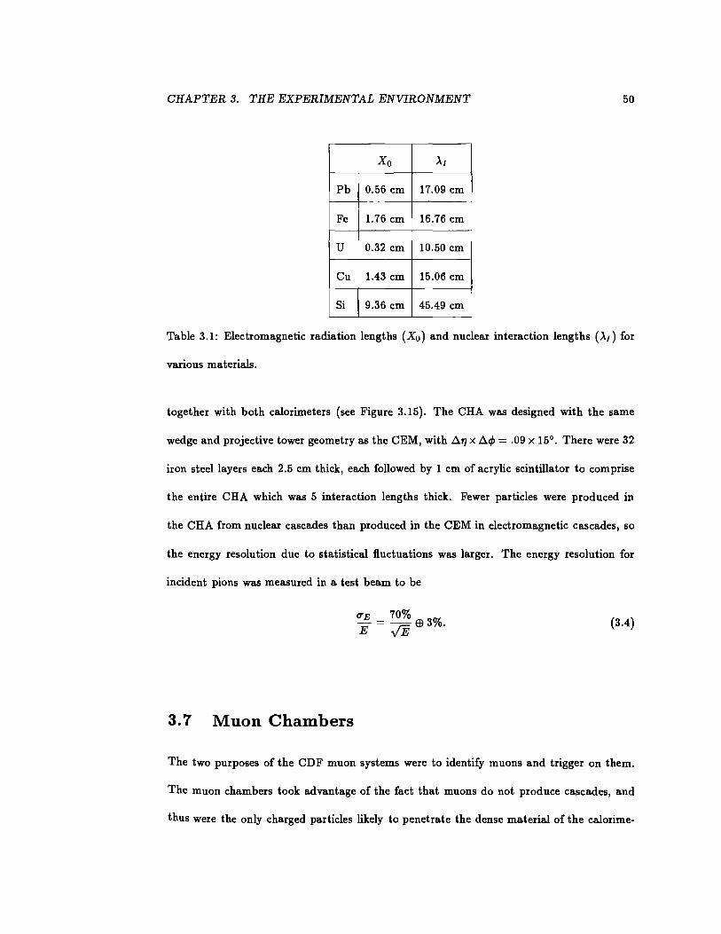
cross section for hadronic interactions. Table 3.1 shows the electromagnetic radiation length
and the nuclear interaction length for a few commonly used absorber materials [4]. It is clear
that many radiation lengths of lead is thin, while having relatively few interaction lengths.
Lead is also cheaper and easier to use than uranium. In hadronic calorimeters, most of the
electrons or photons would already have cascaded, so only the nuclear interaction length
was important. Many nuclear interaction lengths of iron is cheaper and not as heavy as
some of the other materials, so is useful for hadronic calorimeters. For these reasons, lead
was used in the CEM while steel was used in the CHA.
Since the CHA was positioned just outside the CEM, the wedge structure was built
CHAPTER 3. THE EXPERIMENTAL ENVIRONMENT 50
Xo AI
Pb 0.56 em 17.09 em
Fe 1.76 em 16.76 em
u 0.32 em 10.50 em
Cu 1.43 em 15.06 em
Si 9.36 em 45.49 em
Table 3.1: Electromagnetic radiation lengths (Xo) and nuclear interaction lengths (AI) for
various materials.
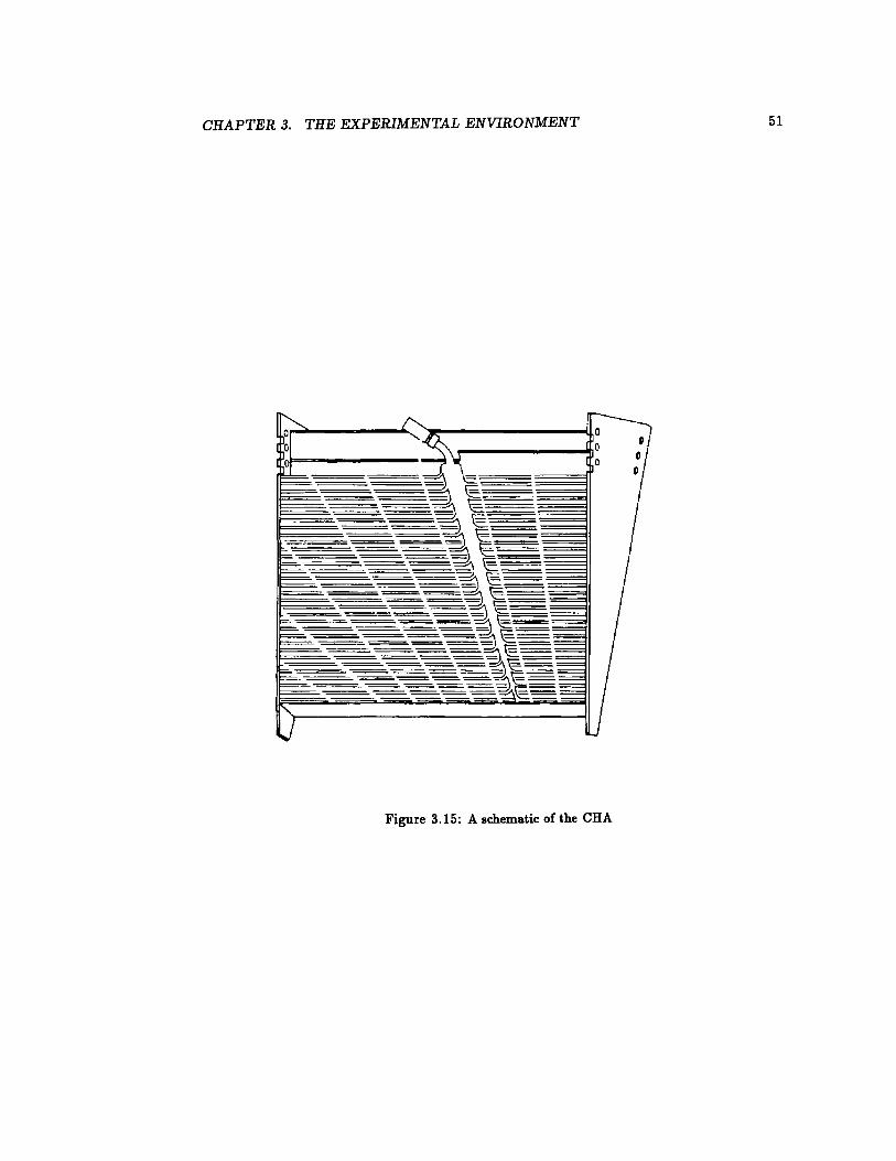
together with both calorimeters (see Figure 3.15). The CHA was designed with the same
wedge and projective tower geometry as the CEM, with ll1J x ll¢ = .09 x 15°. There were 32
iron steel layers each 2.5 em thick, each followed by 1 em of acrylic scintillator to comprise
the entire CHA which was 5 interaction lengths thick. Fewer particles were produced in
the CHA from nuclear cascades than produced in the CEM in electromagnetic cascades, so
the energy resolution due to statistical fluctuations was larger. The energy resolution for
incident pions was measured in a test beam to be
(3.4)
3. 7 Muon Chambers
The two purposes of the CDF muon systems were to identify muons and trigger on them.
The muon chambers took advantage of the fact that muons do not produce cascades, and
thus were the only charged particles likely to penetrate the dense material of the calorime-
CHAPTER 3. THE EXPERIMENTAL ENVIRONMENT 51
Figure 3.15: A schematic of the CHA
CHAPTER 3. THE EXPERIMENTAL ENVIRONMENT 52
ters. The development of an electromagnetic cascade follows the emission of an energetic
photon due to the rapid acceleration of an incident charged particle under the influence
of the nuclear Coulomb field. The large mass of the muon compared to that of the elec-
tron greatly reduces the probability of such accelerations. Hence, muons do not produce
electromagnetic cascades. Hadronic cascades, on the other hand, result from hadronic in-
teractions between the incident particle and the nuclei of the material. Since leptons do not
interact hadronically, they do not produce hadronic cascades. Muons then pass through the
calorimeters only mitigated by normal charged particle energy loss and multiple coulomb
scattering.
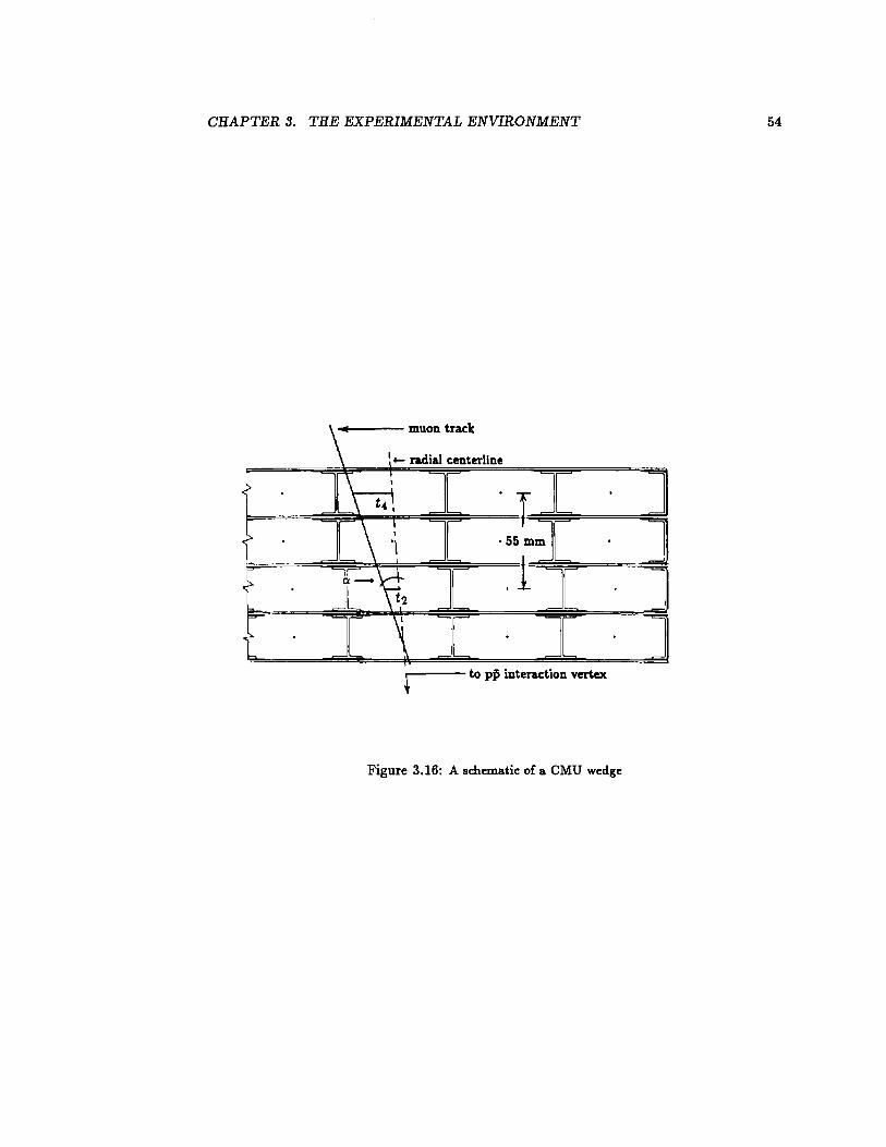
In the central region the muon detection was performed with the Central Muon Detectors
(CMU). The CMU detectors were drift chambers for the detection of charged tracks. There
were 48 sets of chambers, one located behind each CHA wedge. The set of chambers, or
CMU wedge, subtended 12.6° in ¢. This left a gap of 2.4° between each wedge.
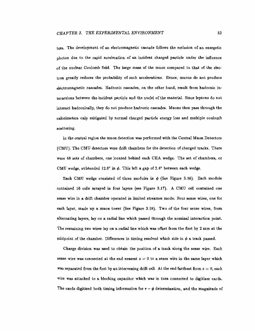
Each CMU wedge consisted of three modules in ¢ (See Figure 3.16). Each module
contained 16 cells arrayed in four layers (see Figure 3.17). A CMU cell contained one
sense wire in a drift chamber operated in limited streamer mode. Four sense wires, one for
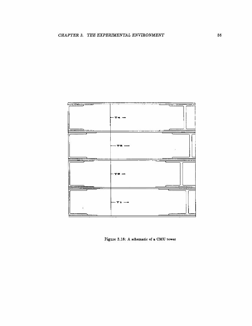
each layer, made up a muon tower (See Figure 3.18). Two of the four sense wires, from
alternating layers, lay on a radial line which passed through the nominal interaction point.
The remaining two wires lay on a radial line which was offset from the first by 2 mm at the
midpoint of the chamber. Differences in timing resolved which side in ¢ a track passed.
Charge division was used to obtain the position of a track along the sense wire. Each
sense wire was connected at the end nearest z = 0 to a sense wire in the same layer which
was separated from the first by an intervening drift cell. At the end farthest from z = 0, each
wire was attached to a blocking capacitor which was in turn connected to digitizer cards.
The cards digitized both timing information for r - ¢ determination, and the magnitude of
CHAPTER 3. THE EXPERIMENTAL ENVIRONMENT 53
the pulse for z determination.
3.8 Luminosity Monitor
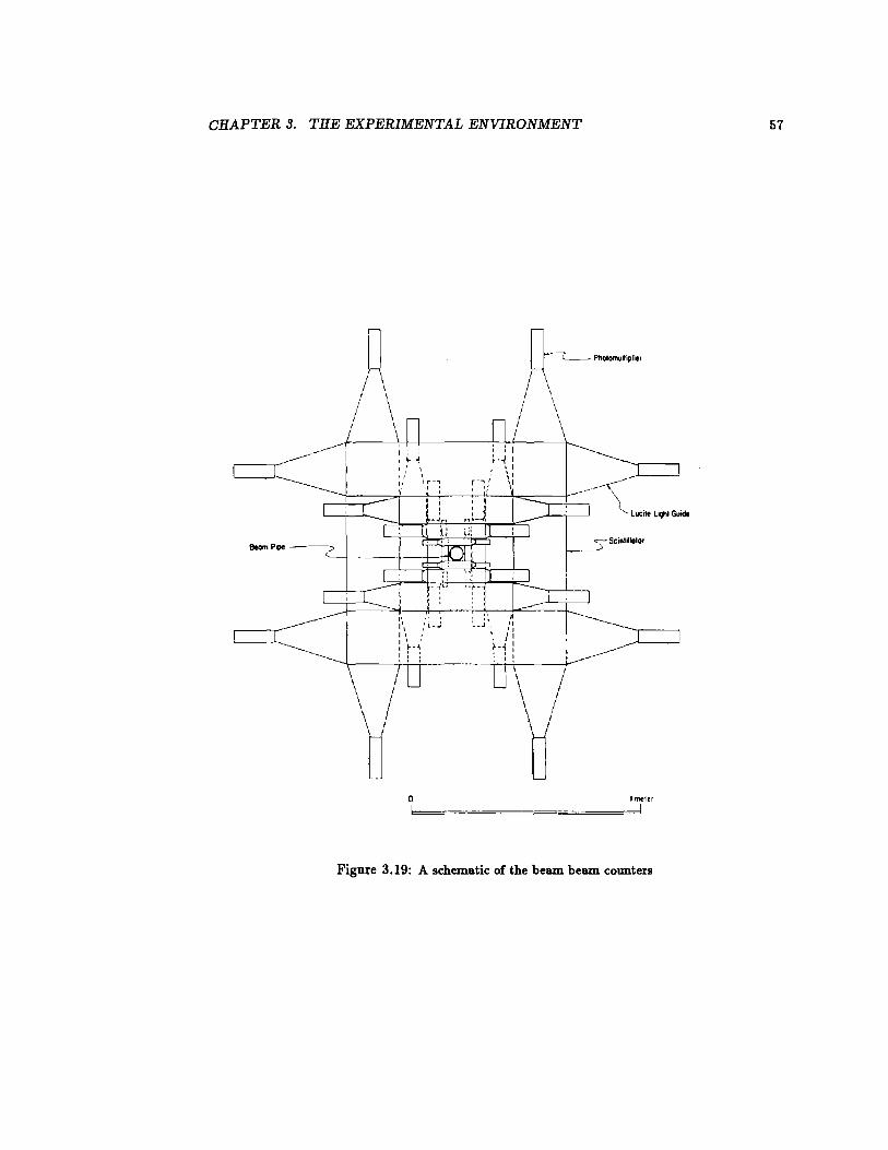
CDF was equipped with a series of low angle scintillators, called the Beam-Beam Coun-
ters (BBC's), which were used as a luminosity monitor. They provided a beam luminosity
measurement independent of that obtained strictly from measurements of beam profile pa-
rameters. These planes of scintillator, with the geometry outlined in Figure 3.19, surrounded
the beampipe on both sides of the detector. The BBC active region was 0.32° < 0 < 4.47°.
The time information from the BBC's had a resolution ofless than 200 ps, and thus gave a
measurement of the time of the interaction.
3. 9 Data Collection
The data used in this analysis were collected over a 12-month period in 1988 and 1989. The
peak machine luminosity grew to over 2 x 1030 cm-2 s- 1 by the end of the run. Although
4.7 pb- 1 were taken for the run, only 2.6 pb- 1 were taken utilizing the dimuon trigger
described in the next chapter.
CHAPTER 3. THE EXPERIMENTAL ENVIRONMENT 54
\ muon track
1 - radial centerline
> \ \
~
_\t;l, '+ ;. \ ·\ ·55m~J[ J r 1-~2 .1 ~
tz
~ \ .
~r---- to pp interaction vertex
Figure 3.16: A schematic of a CMU wedge
CHAPTER 3. THE EXPERIMENTAL ENVIRONMENT
~y X
MUON CHAMBERS
I I 2260 l:nl:n
CENTRAL CALORIMETER
WEDGE
4> e
Figure 3.17: A schematic of a CMU wedge
55
CHAPTER 3. THE EXPERIMENTAL ENVIRONMENT 56
"
~T4- D I
r----r:s-
~
-TI2-
~
f--'T1 -
' '--
Figure 3.18: A schematic of a CMU tower
CHAPTER 3. THE EXPERIMENTAL ENVIRONMENT 57
KC __ Pholonwlliplier
i \
0
Figure 3.19: A schematic of the beam beam counters

Chapter 4
Triggering
In the hadron collider environment at the Tevatron, the collision rate was 105 times higher
than the rate at which the detector could be read out. Because ofthis, a way of selecting the
interesting events was required. To quantify more precisely the reduction needed, it should
be noted that the inelastic cross section in jip collisions at Tevatron energies is about 40
millibarns, whereas the charmonium cross section for the region addressed in this analysis
is measured in nanobarns. Since the instantaneous luminosity at CDF averaged about 1.6
p.b- 1s-1 , the inelastic collision rate was about 70 kHz. The maximum rate for reading
events out of the detector and writing them to tape was a few Hertz. Therefore, there was a
great need to select or reject events in an intelligent manner. The method of making a quick
decision on whether a given event is interesting is called triggering. The selection criteria
for making this decision is called a trigger. A trigger is needed to do most kinds of physics
at a hadron collider.
To accumulate a well defined sample of interesting physics events while rejecting other
kinds of events, CDF employed a four level trigger system [33) to reduce the interaction rate
58

CHAPTER 4. TRIGGERING 59
to a rate that could be written to tape. Many sets of triggers with different selection criteria
for many different topics were used. These topics ranged from top quark tagging and vector
boson selection to jet analyses and charmonia production. The trigger specifically described
here for the Xc analysis was aimed at selecting the dimuon decay of the J /1/J. It should be
kept in mind that the total trigger system at CDF had a much more general nature. Bearing
that in mind, the trigger system and the dimuon trigger are described below.
The purpose of the multi-level structure of the trigger was to make trigger decisions
while introducing as little unwanted bias as possible at the lower levels. Each level of the
trigger needed to reduce the rate to a point where the next level could do a more complex
analysis without incurring significant deadtime. Each successive level of the trigger used
more information and took more time making the decision. The first three levels, denoted
level 0, level 1, and level 2, were hardware triggers. They used analog signals representing
a subset of the information available from a full detector readout. The highest level trigger,
level3, was performed on an ACP farm (a farm of60 Motorola 68020 computer nodes, named
for Advanced Computer Program (34]). The computers ran with Fortran algorithms, with
the full detector data available. Due to the cleanliness of the dimuon signal, the level 3
trigger was not needed to select the data sample for this analysis.
The dimuon selection criteria for this analysis, for reasons which will become apparent
shortly, was labelled the dimuon_central_3 trigger. This trigger was implemented during
only a portion of the 1988-89 run, so it gathered data from an integrated luminosity of only
2.6 pb-1 and not the 4. 7 pb- 1 of the entire run.
The first level of trigger selection, the level 0 trigger, was designed to select inelastic
events. It did this by requiring at least one beam-beam counter (BBC) hit in both the
forward and backward counter arrays coincident within a 15 ns window centered on the
beam crossing time. A crude (± 4 em) measurement of the vertex position was also obtained
CHAPTER 4. TRIGGERING 60
from the timing. Level 0 had 3.5 microseconds to decide whether to pass the event to the
next trigger level before the next crossing. The small time the decision actually took (~
500 ns) resulted in no dead time. That is to say that no beam crossing was wasted while
the level 0 trigger "made up its mind". The trigger decision was available in time to inhibit
data taking during the next beam crossing, 3.5 p,s later.
The level 1 decision was made within the 7 p,s allowed by level O, including the 3.5 p,s
level 0 decision time. If the event failed in level 1, the front end electronics were reset in
time for the second crossing after the initial level 0 decision. The level 1 dimuon trigger
made decisions based upon information from the muon trigger towers indicating that there
was at least one central muon candidate in the event.
The level 1 muon trigger used hits from the muon TDC's to identify high PT track
"stubs" in the muon chambers. The trigger imposed a cut on the time difference jt4- t21 or
jt3 - t 11 (See Figure 3.18) between two radially aligned wires in a muon tower, where t; was
the drift time to the ith wire in the muon tower (35]. This restricted the maximum allowed
angle of a track with respect to an infinite-momentum track (straight in the magnetic field)
emanating from the pfJ vertex and thus applied a cut on the PT of the muon candidate.
Multiple scattering softens the trigger threshold in muon candidate 'PT· This is due to
the smearing of the angle with which the track passes through the muon chamber. The
nominal angle for a muon travelling from the origin to the CMU is ao ~ ~. where Ca0 PT
is a constant arising from the geometry and magnetic field. The angle, a 0 , is smeared in
a way which can be approximated by a Gaussian with a width as described in Chapter 8.
If f:l.t is defined as the minimum of jt4 - t2i or jt3 - t1l, for a muon it would nominally be
related to the transverse momentum by .6.t0 ~ cA•o. Since the level 1 trigger imposed a PT
maximum of 70 ns on f:l.t, the angle used in this trigger corresponded to aPT threshold of
3 GeV /c. The sharpness of this cut is lost, however, due to the spread in f:l.t from multiple
CHAPTER 4. TRIGGERING 61
scattering.
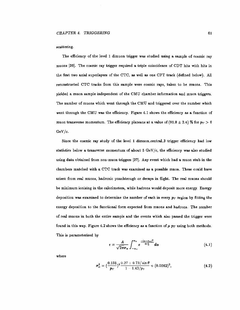
The efficiency of the level 1 dimuon trigger was studied using a sample of cosmic ray
muons (36]. The cosmic ray trigger required a triple coincidence of CDT hits with hits in
the first two axial superlayers of the CTC, as well as one CFT track (defined below). All
reconstructed CTC tracks from this sample were cosmic rays, taken to be muons. This
yielded a muon sample independent of the CMU chamber information and muon triggers.
The number of muons which went through the CMU and triggered over the number which
went through the CMU was the efficiency. Figure 4.1 shows the efficiency as a function of
muon transverse momentum. The efficiency plateaus at a value of (91.8 ± 2.4) %for PT > 6
GeV/c.
Since the cosmic ray study of the level 1 dimuon_central_3 trigger efficiency had low
statistics below a transverse momentum of about 5 Ge V / c, the efficiency was also studied
using data obtained from non-muon triggers (37]. Any event which had a muon stub in the
chambers matched with a CTC track was examined as a possible muon. These could have
arisen from real muons, hadronic punchtrough or decays in flight. The real muons should
be minimum ionizing in the calorimeters, while hadrons would deposit more energy. Energy
deposition was examined to determine the number of each in every PT region by fitting the
energy deposition to the functional form expected from muons and hadrons. The number
of real muons in both the entire sample and the events which also passed the trigger were
found in this way. Figure 4.2 shows the efficiency as a function of JL PT using both methods.
This is parameterized by
A lac € = .J21rua -ace
-(a-ag )2
'""~ da (4.1)
where
2 (0.131) 2 0.27+0.73/sinB ( )2 O'a = -- _ 1 43 / + 0.0062 ,
PT 1 . • PT (4.2)
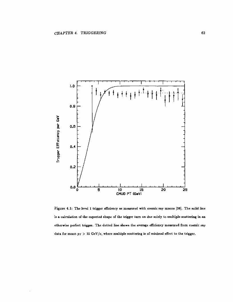
CHAPTER 4. TRIGGERING 62
1.0
0.8
I I 1 I I ti I 1tlljjlfl
> CD to '-CD 0.6 ~ .... u c: CD ... u .... t:: 0.4 LIJ '-CD C" C" ... '-1-
0.2
5 10 15 20 25 CMUO PT CGeVl
Figure 4.1: The level 1 trigger efficiency as measured with cosmic ray muons [36]. The solid line
is a calculation of the expected shape of the trigger turn on due solely to multiple scattering in an
otherwise perfect trigger. The dotted line shows the average efficiency measured from cosmic ray
data for muon PT > 15 GeV /c, where multiple scattering is of minimal effect to the trigger.
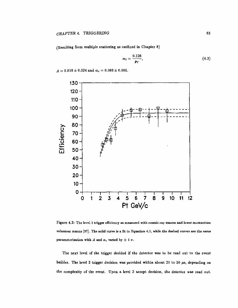
CHAPTER 4. TRIGGERING 63
(Resulting from multiple scattering as outlined in Chapter 8)
0.126 ao= --,
PT (4.3)
A= 0.918 ± 0.024 and ac = 0.086 ± 0.005.
130 120 110 100 ------· 90 ------·
>- 80 (..) c 70 Q) ·- 60 u ·-'+-w 50
40 30 20 10 0
0 1 2 3 4 5 6 7 8 9 10 11 12 Pt GeV/c
Figure 4.2: The level1 trigger efficiency as measured with cosmic ray muons and lower momentum
volunteer muons [37]. The solid curve is a fit to Equation 4.1, while the dashed curves are the same
parameterization with A and ac varied by ± 1 u.
The next level of the trigger decided if the detector was to be read out to the event
builder. The level 2 trigger decision was provided within about 20 to 30 p.s, depending on
the complexity of the event. Upon a level 2 accept decision, the detector was read out.
CHAPTER 4. TRIGGERING 64
Readout took just over 1 ms and incurred less than 10 % deadtime. The level 2 dimuon
trigger included muon stubs (the level 1 central muon candidates) and CTC tracks found
by the Central Fast Tracker (CFT), a hardware track processor [38] which detected high
transverse momentum tracks with fast timing information from the CTC.
The CFT identified tracks by analyzing prompt hits from the axial sense wires of the
CTC. These hits were compared to predetermined hit patterns for the range of transverse
momenta allowed by the CFT trigger threshold. The processor covered the PT range above
2.5 GeV jc. For tracks 2.5 GeV jc < PT < 15 GeV jc, the CFT provided a momentum
resolution of approximately 3.5% x( 1 a"tv1J 2 . The CFT was designed to find tracks in
PT regions, the highest region for all tracks with PT > 15 GeV jc. Thus the CFT had no
momentum resolution above PT > 15 GeV jc. The list of tracks found was available for use
in level 2 triggers.
When the CFT finished the pattern recognition procedure, it sent a list of tracks to a
hardware system called the muon match box. The muon match box contained lookup tables
stored in read-only memory to match the CFT tracks to level 1 muon stubs. The lookup
table was designed to take into account the magnitude of such effects as track curvature
and multiple scattering of charged particles traversing the calorimeters on the way to the
muon chambers. If a level 1 muon candidate stub matched a CFT track, a match defined as
consistent with pointing to the same muon wedge, a bit was set in an fl¢ map which labelled
the muon candidate as a "gold muon". This map was merely an array of bits corresponding
to each muon wedge. There were 24 muon wedges around the detector in 2 separate 11
regions, so there were 48 bits available in the map.
This map of gold muons was then processed by a device called the gold muon cluster
finder. This cluster finder's purpose was to merge gold muon candidates which were in
adjacent muon wedges into a gold muon cluster. This had the effect of turning 2 real muons
CHAPTER 4. TRIGGERING 65
into one gold muon candidate if they were in adjacent wedges. Muon wedges were defined
as adjacent in cp if on the same 11 side of the detector or adjacent in 11 if in the same cp region.
This merging minimized the rate from jet events with more than one track from jet activity
leaking into the muon chambers, while keeping most of the actual dimuon rate. The level 2
dimuon_central_3 trigger required two or more gold muon clusters.
The level 2 dimuon_central_3 trigger, in summary, consisted of the following require-
ments; 1) 2 level 1 muon trigger stubs in the event, 2) the CFT track associated with the
muon stubs must have a transverse momentum greater or equal to 3 Ge VIc, and 3) at least
two gold muon clusters. This had the effect of excluding muons which were in adjacent
wedges in 11c/J as described above.
The level 2 dimu_central_3 trigger efficiency was studied with data using non-muon and
non-CFT triggers [37]. The efficiency for the CFT to tag muon candidates which had passed
the level 1 muon trigger was measured beginning with a muon stub which triggered at level
1, and had an associated CTC track. Information from the muon matchbox tables was
examined to see if CFT tracks had been associated with the candidate. The CFT efficiency
for muons with 'PT > 3 GeV lc was found to be (99.5 ±8:~)%. For events with two muon
stubs with PT > 3 Ge VIc, both of which passed level 1 and which satisfied the non-adjacent
geometry, the number of events which actually passed the level 2 dimu_central_3 trigger was
examined. This resulted in a measured efficiency of (98.5 ±~:8)%, consistent with the CFT
efficiency for both muon candidates.
Level 3 cuts were not needed for this trigger. The level 3 trigger was a software trigger,
which ran from Fortran source code on nodes of a computer network. The algorithms
selected on complicated quantities and filters, and reduced the trigger rate by keeping good
trigger events. Since the dimuon rate was low, and the signal relatively clean, there was no
need to include more complicated cuts for the dimuon_central_3 trigger.
Chapter 5
OfHine Reconstruction
The offline reconstruction identified particles from tracks in the wire chambers and energy
depositions in the calorimeters. The data from the detector was analyzed to find events with
properties consistent with jets, electrons, high energy photons, muons, etc. Those features
of an event consistent with objects of interest were called physics object candidates.
Physics object candidates were defined according to different criteria depending on the
object desired. For instance, a central muon candidate object, or CMUO, was defined as
a CMU stub matched with a CTC track. This matching was performed by extrapolating
the CTC track to the muon chamber position. The extrapolation included the effects of the
magnetic field inside the solenoid, the return yoke and the calorimeters. It took into account
multiple scattering and energy loss in the material traversed. A central photon candidate
was identified by the presence of energy in a central electromagnetic calorimeter tower,
accompanied by clusters of energy in both views of the associated central strip chamber.
Since the reconstruction of the reaction Xc --+ J /1/J"Y, J /1/J --+ JL+ JL- is the subject of this
analysis, JL and "Y candidates will be emphasized.
66
CHAPTER 5. OFFLINE RECONSTRUCTION 67
The offiine reconstruction included a complex series of algorithms to find these physics
object candidates. The algorithms could find the interaction z vertex for the event (and/or
the number and positions of such vertices if there were more than one), the charged tracks
in the CTC, the energy deposition in the calorimeters, and the CMU stubs. They could
also combine information from different parts of the detector, as in, for example, linking the
CMU stubs with CTC tracks.
5.1 Event Vertex Determination
The offiine analysis began by finding the z location ofthe event along the beam line. This was
the first step because it was important for many other parts of the offiine reconstruction. For
example, the z vertex was needed for CTC track parameterization, beam vertex constraints,
and ascertaining photon direction. The interactions had a large spread in z because the p and
p beam bunches were long. The intersection of these bunches was such that the distribution
of event vertices at the BO interaction point in the Tevatron collider was well described by
a Gaussian along the beam axis with a standard deviation in the z direction of 30 em, as
shown in Figure 3. 7. The subdetector specifically designed for the purpose of event vertex
determination was the VTPC (see section 3.3).
The process of z vertex determination started with finding VTPC track segments. The
hit patterns ofthe wires in each VTPC octant of each segment were examined for consistency
with coming from a charged particle track (or tracks). Since most tracks were straight in
an octant, this was a relatively simple reconstruction. In addition, the number of hits in
a given octant was small, resulting in a low number of possible combinations. A VTPC
track segment was defined by the following requirements. First, the number of wires with
hits in an octant was required to be greater than five. Second, the hit occupancy for the
CHAPTER 5. OFFLINE RECONSTRUCTION 68
region containing the track was required to be greater than or equal to 70 percent. Third, the
residuals of the hit positions, calculated as described in section 3.3, from the track path were
used to calculate a x2 • The uncertainties used in the x2 calculation were underestimated
by a factor of 1.5 to 2.0 [39]. Since· the average number of hits was 24 per track, the x2 for
most tracks averaged around 100. This x2 was required to be less than or equal to 1000 for
a good track, which rejected only extremely poorly measured tracks. The entire VTPC was
searched until all VTPC track segments were found.
Once all of the VTPC tracks were identified they were grouped together to find the
common vertex of the event, or events if two pP collisions had occurred. Each VTPC track
segment necessarily had a z intercept, defined as the position of the point on the track closest
to the z axis. These z intercepts from all of the tracks were clustered into sets to form z
vertex candidates with no more than 2 em separating nearest neighbors. Each cluster would
become a vertex candidate. A new cluster was started if the z intercept of a VTPC track
segment was greater than 1.5 em from the center of the cluster. Once all z intercepts were
assigned a cluster, a 1.5 em window was found which maximized the number of intercepts in
that window. The average z was calculated for each cluster window. Then all of the tracks
were compared to these cluster centers and reassigned (to a new cluster) if they fell within
the 1.5 em window. This process was iterated until the mean of the z intercepts was within
± 1 em of the previous mean. If a track fell within 1.5 em of two separate clusters, it was
assigned to the closest. The cluster with the largest number of segments used in the fit was
chosen as the primary event vertex.
The efficiency of this algorithm was checked by scanning events. For the sample of
minimum bias events which was examined, the efficiency for correctly locating the z vertex
of the event was determined to be (98±i:3 ) %. Minimum bias events were all events resulting
from a prescaled trigger consisting of only BBC hits in time with the beam collision time

CHAPTER 5. OFFLINE RECONSTRUCTION 69
(a level 0 trigger alone). For a sample of physics specific triggers selecting high ]JT, high
energy, or high multiplicity events, the scan established that the efficiencies for correctly
locating the z vertex was (99 ±:l) %. The resolution of the z vertex as determined by the
algorithm was determined to be about 2 mm by dividing the spread of the cluster by the
square root of the number of tracks in the cluster.
A subtlety which was glossed over to this point in the reconstruction and deserves expla-
nation is how the beam location itself was defined. The z vertex position found above gave
only the z coordinate of the interaction vertex. However, the location of the beam varied in
:z: and y from run to run. The exact path of the beam for each run was determined (by a
method described below), and could be combined with the z vertex information to find the
position of the event vertex.
5.2 Charged Track Finding
The trajectories of charged particles were found by examining CTC information. The list
of hit wires and the associated drift times was the starting point of the track finding. For
each hit sense wire, the drift timet, coupled with the drift velocity vd, and the global event
time t 0 , defined two points in space, equidistant from the wire at ±d = vdlt- tol along the
drift trajectory for the wire.
The next step in tracking was pattern recognition. This grouped hits consistent with
arising from a single particle's ionization track into a list of tracks. It was natural to begin
the pattern recognition by finding track segments in each drift cell, since there were a limited
number of hits per cell. Also, higher PT tracks yielded relatively straight small segments.
Since the time left an ambiguity as to which side of the sense wire the ionization occurred, a
track would leave two segments with symmetry around the sense wire plane. This ambiguity

CHAPTER 5. OFFLINE RECONSTRUCTION 70
was resolved when the segments were linked into tracks.
The pattern recognition algorithm then linked the segments together by starting at the
outer axial superlayer and examining "roads", or bands of probable particle trajectories
which could produce the drift cell track segment. The road was computed from the segment
center going to the origin, and took into account the slope of the track segment. Axial
superlayers along the r - ¢ plane road were examined for segments which were consistent
with the trajectory hypothesis. The roads were re-calculated or dropped at each successively
smaller layer. Finally, when the inner axial superlayer was reached, the stereo layers were
examined, outer to inner, for segments resulting in a helical road.
At this point, there was a list of tracks which included the hits used in each track. The
side of the drift wires of each hit should have been determined by which segment hypothesis
remained in a track. Thus the list of hits was a list of points in space associated with each
track. Hits were allowed to be associated with multiple tracks, up to the number of found
tracks which passed through the drift cell.
The final step of tracking was a fit of the helix track parameters to the list of hits for
each track. A charged track helix in the CTC must have been co-axial with the magnetic
field, and thus it could be completely specified by the following variables:
• R, the signed radius of the helix (R = ±IRI). The sign is the sign of the charge of the
particle
• cot 8, where 8 is the pitch angle of the helix
• zo, the z position of the closest approach of the helix to the z axis, nearest the primary
vertex
• do, the distance in the a: - y plane from the z axis to that same point of closest
approach
CHAPTER 5. OFFLINE RECONSTRUCTION 71
• ¢0 , the ¢ angle ofthe tangent to the helical track at that same point of closest approach.
The fit included all hits which were in the hit list for the track, provided they were acceptably
close to the helix parameters, according to a complex heuristic algorithm [40].
The fit could also include the beam line position (as determined below). This was useful
for tracks which came from the primary event vertex because the increased lever arm resulted
in better determination of the curvature as well as cot 9. This beam-constrained fitting was
used for the events including dimuons from the J /1/J sample. Even though some of the J /1/J
came from long-lived b-flavored hadrons, the decay length would have been around 200 11-m,
while the resolution of the CTC track extrapolations to the beam vertex was similar. In the
absence of a vertex detector, beam constrained tracking gave better resolution.
For tracks which were not expected to come from the primary vertex, such as conversion
candidates or K, --+ 11'+11'- decays, the beam constraint was not used. The tracking using
only CTC hits was called un-constrained tracking. However, due to the pattern recognition
using the primary vertex to define roads, some bias in track parameters toward the primary
vertex was retained, as will be briefly discussed in Chapter 6.
As mentioned previously, the radius of the helical track of a charged particle travelling
in a magnetic field is related to the transverse momentum of the particle. This leads to the
relation with the radius of the helix
Pr = clqBIIRI (5.1)
where c is the speed of light, q is the charge of the particle, and B is the magnetic field
strength. Other relevant quantities could also be derived from the track parameters, such
as
Pz = Pr cot 9 (5.2)
CHAPTER 5. OFFLINE RECONSTRUCTION 72
and the momenta at the point of closest approach
Px = PT cos¢o (5.3)
Py = PT sin ¢ 0 . (5.4)
The resolution due to the finite measurement resolution was QE.r.. ~ 0.0020PT for isolated PT
tracks (PT in GeV /c) if the track traversed all of the superlayers. With a beam constraint,
which added length to the lever arm, this became QE.r.. ~ 0.0011PT [41]. There was also a PT
term due to multiple scattering, which allowed the PT resolution to be parameterized by [42]
(5.5)
The resolution for cot() was estimated to be o cot() ~ 0.003 for unconstrained tracks, and
~ 0.002 for beam constrained tracks [43].
5.3 Determination of Beam Line Position
The beamline did not traverse the detector exactly through the origin or exactly parallel to
the z axis. There were actually an offset and slope, which were run-dependent. Although
the beam profile was smaller than the single event primary vertex resolution, the tens of
thousands of events in a run could be used to fit the beam line parameters for the run.
These beam line parameters could be used, in conjunction with the z position of the event
vertex, to provide the a: - y position of an interaction with a much better resolution than
possible with only information from the tracks from that single interaction.
All CTC tracks consistent with coming from the primary vertex of any event were used
to determine the run by run beam offsets and slopes. These could be used to determine
the a: and y position of the primary vertex from the z position of the vertex as determined
from the VTPC information. This was done to find the point of origin for photons from the
CHAPTER 5. OFFLINE RECONSTRUCTION 73
decay Xc-+ J /1/ry, which was useful in determining the photon direction vector as described
in Chapter 8.
5.4 Central Muon Object Reconstruction
The central muon object (CMUO) reconstruction was performed to find muon candidates
in the CMU detectors. The CMUO identification began with finding track segments in the
CMU, as described below. Once good track segments were found, these were associated
with CTC tracks.
5.4.1 Central Muon Track Stubs
The CMU track segment (CMUS) finding algorithm reconstructed the position and direction
of charged particle tracks in the central muon detectors. Tracks were first found in the r- ¢
plane, as described below. Then, r- z plane tracks were found. Finally, the two views were
matched to form the track segments, also known as muon stubs.
Tracking in the r - ¢ plane began with the number of found TDC hits in each wedge
( 7tT DC) to define track candidates, then fit the hits to a track. If the number of hits was
less than two, the wedge had no CMU track segments. If 7tT DC = 2, there was a possibility
that the hits were from an isolated muon. If the two hits were in different layers, and in cells
that were separated by fewer than two cells in the r - ¢ direction, the hits were assigned
to two track candidates. There were two track candidates because with only two hits the
ambiguity of which side of the drift cell the track was on could not be resolved.
If nTDC > 2, tracks were found via a more complicated method. If more than one
layer had no TDC hits, no track was found, but if at least three layers had hits, the search
continued. Every combination of two hits separated by two layers defined extrapolated lines
CHAPTER 5. OFFLINE RECONSTRUCTION 74
for a possible track candidate. The other planes were checked for hits within a road of 0.25
em in the r - ¢ coordinate, which was about 10 standard deviations on the hit position.
If at least one hit from the other layers was within the road, the hits were assigned to a
track candidate. If all the hits used in a track were in the same cells as those in another
track candidate, the duplicate candidate (the second track found by the algorithm in these
cells) was dropped. If wrve < 6, it was assumed only one track was present, otherwise
the tracking process was iterated over all pairs of tracks separated by two layers, up to a
maximum of 75 track candidates. The hits for each track were then fit to a line, which
resolved the ambiguity of which side of the drift cell the track occurred.
The r - z plane tracks were then found with a method similar to the above, but using
the number of ADC hits (nAve). If nAve was less than two, no tracks were found in the
wedge. If nAve = 2, and the cells were at least adjacent in the r- ¢direction, r- z tracks
were fit. If nAve > 2, and the hits were in at least three different layers, roads of width
5.0 em (about 10 standard deviations in the r- z coordinate) were searched for any hits. If
there were any, the hits for each track (up to 75 tracks) were fit to a line.
The last stage of muon stub reconstruction matched the tracks in the two views. If
the tracks in the two views shared at least two cells, they were matched and provided a
CMUS. For any leftover r - ¢ tracks which remained unmatched, hits in the r - z plane
were re-examined for the possibility of providing a lower quality r - z track. If hits in the
r- z plane (which showed no track) fell in any two cells with r- ¢ hits from the leftover
track, a new r - z track was constructed and matched to the r - ¢ track.
5.4.2 Linking CTC Tracks to Muon Stubs
Once track segment stubs were found, the CMUS stubs were associated with CTC tracks,
beginning with the tracks. Each CTC track with PT > 1 GeV Jc was extrapolated to the
CHAPTER 5. OFFLINE RECONSTRUCTION 75
CMU position. Tracks below a transverse momentum of about 1.4 GeV /c were expected to
range out in the calorimeter and never reach the muon detectors. The position calculation
included a nominal dE /dz for a minimum ionizing track traversing the coil and calorimeters.
The effects of the return field through the CHA were also included in the extrapolation. In
the dE/ dz calculation, and the track extrapolation, multiple scattering was not modelled,
but the calculation of the uncertainties in the extrapolated position did include the effects
of multiple scattering.
Tracks from decays in flight prior to the CTC were expected to have large impact pa-
rameters relative to the fJp beams. To exclude most of these from the matching procedure,
an impact parameter requirement of 1.0 em or less was imposed.
Each extrapolated track which had enough momentum to reach a CMU wedge was
considered a candidate for matching to any stub in that wedge. The extrapolated position
and slope in the CMU was calculated for track-stub linking. A x2 was determined from the
residuals in position and slope weighted by the multiple scattering deviations expected for
a 1 GeV jc particle. This was done, instead of a x2 based on the actual momentum of the
track, in order to minimize bias against high momentum tracks. High momentum tracks
would have had lower deviations from multiple scattering, thus a falsely high x2 if the muon
chamber were slightly mis-aligned with the CTC. The track which matched the position and
intercept in the CMU of the muon stub with the best x2 in the r- tjJ plane was retained as a
muon candidate. However, if a track propagated near the tjJ crack between wedges (defined
here as more than 35 em from the center of the wedge), it was checked for a match with
any stubs in both wedges.
The muon candidate, consisting ofthe CMUS and CTC track, was then required to have
a transverse momentum greater than 2.0 GeV jc. Muons with a transverse momentum of
less than 1.4 GeV /c would, on average, lose enough energy that they would stop before
CHAPTER 5. OFFLINE RECONSTRUCTION 76
reaching the muon chambers. In addition, the CFT trigger was not fully efficient below
PT = 2.0 GeV /cas shown in Chapter 4. However, some real muons with PT < 2.0 GeV /c
would pass the muon triggers and make it to the muon chambers. To avoid matching
muon stubs from these slow muons with other, higher momentum tracks in the event, the
extrapolation process began with tracks with PT more than 1.0 Ge V / c as outlined above,
while the 2.0 GeV /c cutoff was not imposed until after the track-stub matching was complete.
Track-stub pairs passing all the above requirements were labeled as central muon objects,
or CMUO's.
5.5 CES Clustering
The CES was sensitive to electromagnetic showers from electrons and photons. The purpose
of the offline CES reconstruction was two-fold. The finer segmentation of the CES (as
compared to the CEM towers) provided a better position measurement for finding where
the energy was deposited in the tower. This gave direction information for the electron
or photon, and was useful in position dependent energy corrections. Also, the number
of single particle showers and the number of multiparticle showers in a sample could be
determined by examination of the lateral shower profile. For instance, the decay 1!'0 --> "'1"'1
would be expected to produce a wider energy deposition by virtue of the distance between
the photons when they reached the calorimeter. The CES reconstruction found the position
of the shower, and provided a measure of the lateral shower profile.
Since the channel width of the strip chambers was so thin, CES energy deposition was
grouped into clusters to find positions and shower profiles. This clustering proceeded sep-
arately in the strip and wire views. The CES reconstruction algorithm had three major
facets:

CHAPTER 5. OFFLINE RECONSTRUCTION 77
• the selection of seed channels about which to define a cluster,
• the cluster definition, a decision on which channels belong to a given cluster, and
• the measurement of the cluster energy.
After CES channels were clustered, a fitting procedure to find the centroid of the cluster
was performed. Each of these processes is described below.
The definition of seed channels was relatively straightforward. Any channel with an
energy deposition corresponding to more than 0.5 GeV was defined as a seed. The list of
seeds was ordered from highest to lowest in channel energy deposition. The seeds could then
be used to define CES clusters.
The next step in the CES offline reconstruction was the actual cluster definition. The
clustering began with the highest energy seed channel, then proceeded in a descending seed
energy order. A cluster was defined as the 11 channels centered about the highest energy
unclustered seed channel. The algorithm was then iterated for the next highest energy seed
outside a previous cluster. Clusters were allowed to overlap, as long as the seed tower for the
second cluster was outside the first, so a maximum of 5 channels could be shared between
two clusters. The process continued until no unclustered seeds remained. This resulted in
a list of clusters, each with 11 channels, and the seed channel responsible for each.
The cluster energy was found for each cluster. It was calculated as the sum of energy
in each channel of that cluster. An effective threshold of 0.057 GeV deposited per channel
set a limit on the smallest amount of energy which could be considered in the sum. The
value for the threshold was roughly three sigma above the noise distribution for the CES.
Channels below this threshold contributed zero energy to the sum. Furthermore, although
the channel would still contribute to the profile fits described below, it would do so as an
entry of zero energy. Channels in overlapping clusters shared the energy with each cluster in
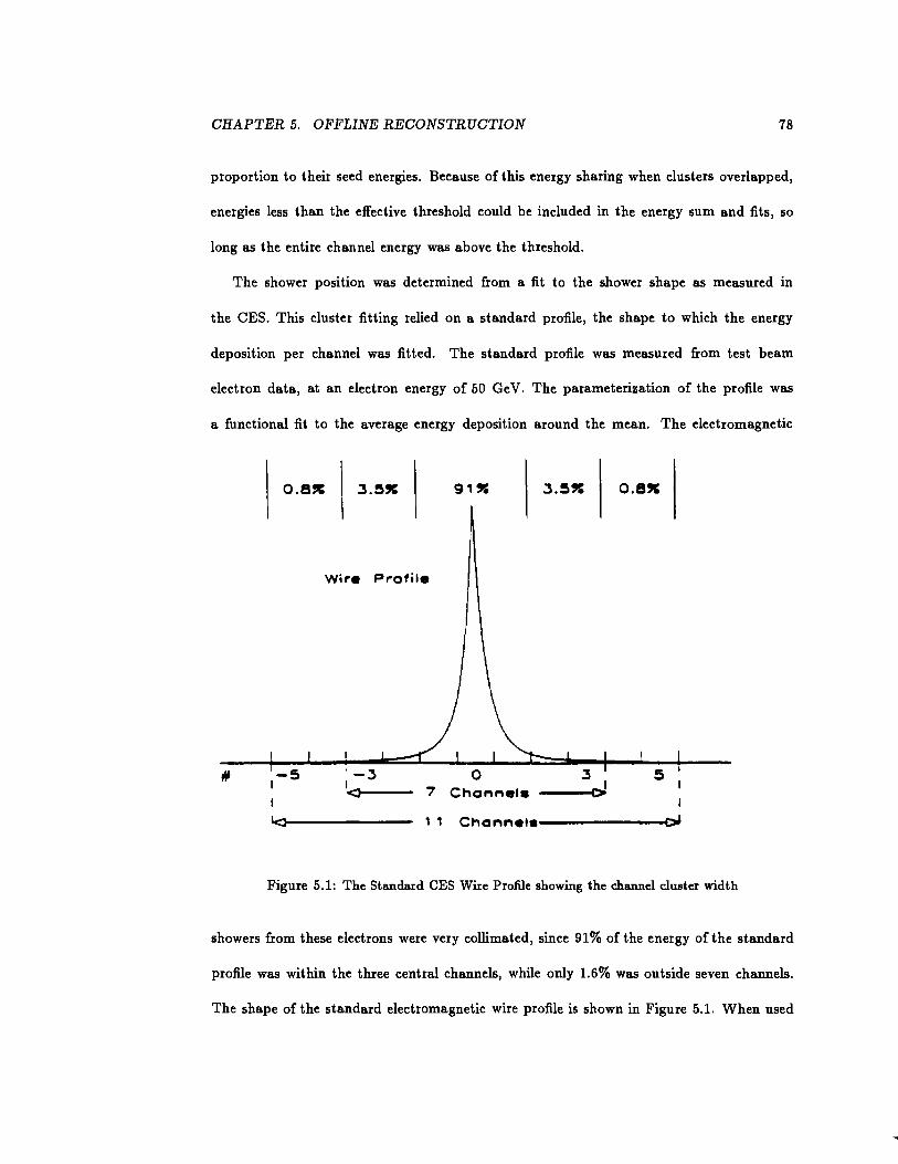
CHAPTER 5. OFFLINE RECONSTRUCTION 78
proportion to their seed energies. Because of this energy sharing when clusters overlapped,
energies less than the effective threshold could be included in the energy sum and fits, so
long as the entire channel energy was above the threshold.
The shower position was determined from a fit to the shower shape as measured in
the CES. This cluster fitting relied on a standard profile, the shape to which the energy
deposition per channel was fitted. The standard profile was measured from test beam
electron data, at an electron energy of 50 Ge V. The parameterization of the profile was
a functional fit to the average energy deposition around the mean. The electromagnetic
o.e~ o.ex
Wire Profile
7 Cnonnela
~------ 1 1 Cno nnela--------C>I
Figure 5.1: The Standard CES Wire Profile showing the channel cluster width
showers from these electrons were very collimated, since 91% of the energy of the standard
profile was within the three central channels, while only 1.6% was outside seven channels.
The shape of the standard electromagnetic wire profile is shown in Figure 5.1. When used
CHAPTER 5. OFFLINE RECONSTRUCTION 79
in the fit, the standard profile was scaled in height so that the area under the parameterized
curve was equal to the cluster energy. The shape parameters other than the height were
independent of cluster energy for test beam electrons with energies from 10 to 100 Ge V.
The measured cluster profiles were then compared to the profile by a CES x2 variable,
testing the quality of the fit. The standard profile, corrected for geometric effects, yielded
a discrete channel by channel expectation E(x;) by integrating the value of the standard
profile parameterization from one channel boundary to the other. The CES x2 was then
calculated by taking the difference between the data and the channel expectation as follows:
2 _ 1 ~ [E;- E(x;)] 2
X--~ 2 4 (]'· i=J I
(5.6)
where i was the CES channel index, E; was the measured channel energy, and (]'~ was the
estimated variance of the profile. The variance (]'t was also parameterized from test beam
electron data [44]. The CES x2 was similar to a standard x2 per degree offreedom variable,
with the exception of the arbitrary normalization of the constant factor of 4, instead of
one less than the number of channels. The factor of 4 was historical, since originally 5
cluster channels had been planned. The number of channels per cluster was increased to
11 to include lower energy 11'0 ----> Ti' in a single cluster, while the definition of CES x2 was
unchanged. The CES x2 thus had a mean value of approximately 2.5 for electron showers.
The fit was performed by allowing the midpoint of the standard profile to float. The
x2 was minimized, and the best center position of the standard profile was the CES cluster
position. Since the standard profile was allowed to be at any position, the CES cluster
position was not constrained to any channel center. This provided a resolution at high
energies smaller than the individual channel size. Figure 5.2 contains the distribution of the
position difference between cluster position and track extrapolated position for electrons,
showing the resolution of the strip chambers was approximately 3 or 4 mm.
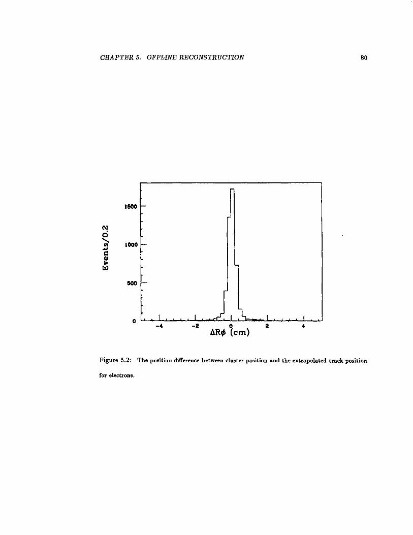
CHAPTER 5. OFFLINE RECONSTRUCTION 80
1&00 I-
N 0
' lOOO I-fl) ~
c:: Q) > tzJ
600 I-
...
0 I I -rl'l\_ L I -4 -2 0
6Rtj) (em) 2 4
Figure 5.2: The position difference between cluster position and the extrapolated track position
for electrons.
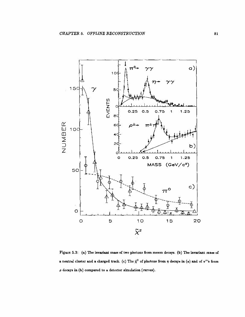
CHAPTER 5. OFFLINE RECONSTRUCTION
15
cr w 10 m 2 =:J z
50
0
0
(/) 1-z w
5
~ 8
6
4
2
-y-y a)
-y-y
b) a~~~~~~~~~~~~~~~~
0 0.25 0.5 0.75 1.25
MASS (GeV/c2)
c)
5 10 15 20
,_2 X
81
Figure 5.3: (a) The invariant mass of two photons from meson decays. (b) The invariant mass of
a neutral cluster and a charged track. (c) The X. 2 of photons from ., decays in (a) and of '1!" 0 's from
p decays in (b) compared to a detector simulation (curves).
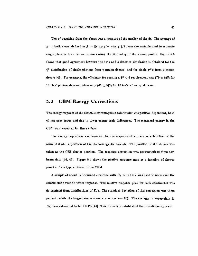
CHAPTER 5. OFFLINE RECONSTRUCTION 82
The x2 resulting from the above was a measure of the quality of the fit. The average of
x2 in both views, defined as :e = [(strip x2+ wire x2 )/2], was the variable used to separate
single photons from neutral mesons using the fit quality of the shower profile. Figure 5.3
shows that good agreement between the data and a detector simulation is obtained for the
:e distribution of single photons from rrmeson decays, and for single 1r0 's from p-meson
decays [45]. For example, the efficiency for passing a :e < 4 requirement was (79 ± 5)% for
10 GeV photon showers, while only (43 ± 5)% for 10 GeV 1r0 --+ "("( showers.
5.6 CEM Energy Corrections
The energy response of the central electromagnetic calorimeter was position dependent, both
within each tower and due to tower energy scale differences. The measured energy in the
CEM was corrected for these effects.
The energy deposition was corrected for the response of a tower as a function of the
azimuthal and z position of the electromagnetic cascade. The position of the shower was
taken as the CES cluster position. The response correction was parameterized from test
beam data [46, 47]. Figure 5.4 shows the relative response map as a function of shower
position for a typical tower in the CEM.
A sample of about 17 thousand electrons with ET > 12 Ge V was used to normalize the
calorimeter tower to tower response. The relative response peak for each calorimeter was
determined from distributions of E jp. The standard deviation of this correction was three
percent, while the largest single tower correction was 8%. The systematic uncertainty in
E fp was estimated to be ±0.4% [48]. This correction established the overall energy scale.
CHAPTER 5. OFFLINE RECONSTRUCTION
N .. X (j)
83
Figure 5.4: Relative response in a central calorimeter tower. The point labeled 1.0 is the point
at which the tower is calibrated; the vertical scale gives the relative response.
CHAPTER 5. OFFLINE RECONSTRUCTION 84
5. 7 Electron Candidates
Electron candidates were reconstructed beginning with a cluster of electromagnetic energy.
The clustering process began by considering all CEM towers with at least 3 GeV of elec-
tromagnetic transverse energy to be seed towers. Transverse energy, cir ET, was defined by
ET = Etower sin (J where Etower was the total electromagnetic tower energy, and (J was the
angle of the line drawn from the tower center to the event vertex with the z axis. Adjacent
towers were added to the cluster if their transverse energy was greater than 0.1 Ge V. In the
CEM, an electron shower was generally contained in one or two towers. Furthermore, the
border between towers in the c/J direction (which contained roughly 1 em of inactive material
as mentioned in Chapter 3) prevented energy from an electron crossing the c/J boundary
between towers. For these reasons, the size of a central EM cluster was restricted to three
or fewer adjacent towers with a common c/J. The cluster was required to have an ET of 5
Ge V or greater to be retained as an electron candidate.
A measure of the lateral shower profile for electron candidates is the variable £,hare· It
was defined to be
(5.7)
where the sum 1s over the towers in the cluster adjacent to the seed tower, Mk is the
measured energy in the adjacent tower, Pk is the expected energy in the adjacent tower,
E is the cluster energy, and t:::..Pk is an estimate of the error in Pk. The expected energy
Pk was predicted using the EM cluster energy, the event vertex, the center of the shower
as measured in the central strip chamber and a shower profile parameterization from test
beam measurements. The uncertainty in the expected energy, t:::..Pk, was taken to be the
variation in Pk arising from a 1 em shift in the center of the shower. The uncertainty in the
cluster energy comes from the resolution ofthe CEM, u(E) ~ 0.14v'E, thus the denominator
CHAPTER 5. OFFLINE RECONSTRUCTION 85
normalized the energy difference Mk - Pk relative to the statistical fluctuations inherent in
the measurement of electromagnetic showers. For most events f:l.Pk was small since the CEM
had full containment (more than 99%) for showers more than 2 em away from a boundary
(the cell size was typically 24 em long in z). The sum was arbitrarily normalized, and gave
a measure of the isolation of the electron candidate . .c. hare was calculated for each central
EM cluster, and was useful for providing a clean electron sample (see Chapter 6).
5.8 Luminosity Measurement
The Beam-Beam Counters provided a measurement of the luminosity delivered by the accel-
erator. This measurement scaled the BBC rate to a known cross section. The cross section
was related to the BBC rate at a lower energy (JS = 546 GeV) combined with accelerator
parameters. The normalization was set by comparing to a UA4 measurement of the frp cross
section at J8 = 546 GeV [49]. The cross section visible to the BBC was calculated to be
O'BBc(at J8 =1.8 TeV) = 46.8 ± 3.2 mb [50]. The BBC rate was monitored, and provided
the measurement of the total integrated luminosity gathered using the dimuon_central_3
trigger of 2.6 ± 0.2 pb- 1 .
Chapter 6
Electromagnetic Efficiency
In the Xc analysis, photons were found using the central electromagnetic calorimeter ( CEM)
energy and the central strip chamber (CES) cluster position. These photons would be com-
bined with J j.,P candidates to find the Xc -+ J /1/J"Y signal. The cross section was calculated
using the various acceptances and efficiencies, including the photon efficiency. The photon
efficiency determination is described in this section.
6.1 Overview of Method
The determination of the photon finding efficiency was done in two parts. First, since
electrons interact electromagnetically in the CEM and CES much like photons, the electron
finding efficiency was measured. This measurement was performed on an unbiased sample
of electrons arising from "Y -+ e+ e- conversions. A check on the calibration of the CEM for
electrons with energies in the range 1 to 5 Ge V was also performed, since the calibration
was designed for energies above 5 GeV. The photon finding efficiency was then found by
correcting this electron finding efficiency for slight differences in the CEM and CES responses
86
CHAPTER 6. ELECTROMAGNETIC EFFICIENCY 87
for photons versus electrons. The calculation of the response differences relied on detailed
modelling of the behaviour of the CEM and CES.
6.2 Conversion Electron Selection
A sample of electrons unbiased with respect to calorimeter response was needed to measure
the efficiency for finding low energy electrons. This sample was obtained from photon con-
version electron pairs, identified by one electron candidate passing the electron calorimeter
cuts and using only tracking information to identify the second electron. The "second"
electron thus provided the required unbiased electron sample.
6.2.1 First Electron Selection
The first electron was chosen with the following selection criteria. First, all electron candi-
dates (as described in Chapter 5) were examined from the inclusive election data sample.
Electrons were expected to lose almost all their energy in the CEM while hadrons were
expected to penetrate to the CHA. The ratio of hadronic energy over electromagnetic en-
ergy was therefore required to be less than 0.05 (this implicitly required the electron to be
isolated from other activity in the event) . .C.hare (as defined in section 5.7) was required
to be less than 0.2 to provide a further isolation cut. The .C.hare distribution is shown in
Figure 6.1, with the peak near zero containing the most isolated electron candidates. The
cut at .C.hare = 0.2 was on the plateau region.
The electron cluster was required to have at least one 3-D track aimed at it; for more
than one such track, both the highest momentum track and the track passing nearest to the
centroid of the CES cluster were used as electron candidates. The ratio of CEM energy to
CTC momentum was required to be between 0.6 and 1.5 to make sure that the CTC track
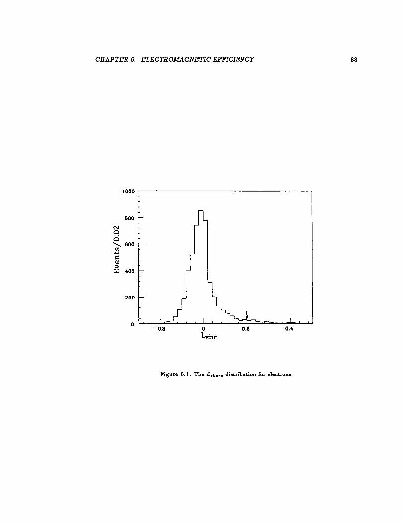
CHAPTER 6. ELECTROMAGNETIC EFFICIENCY 88
800
N 0 0
' 600 rn
...,J
c cu >
tzJ 400
Figure 6.1: The £.hare distribution for electrons.

CHAPTER 6. ELECTROMAGNETIC EFFICIENCY 89
was consistent with the deposited energy ..
6.2.2 Initial Track Selection of Conversion Candidates
Once an electron candidate was chosen, all other tracks were examined for possible use
in the conversion sample. The conversion pair candidates were required to have opposite
charges. Pairs of electrons from a photon converting in the material of the detector would
initially be travelling in the same direction. This fact was used to determine the constraints
necessary to select conversions.
The most readily available check on whether two particles were initially travelling in the
same direction was the difference between the measured value of cot 8 for each track. The
value of cot 8 did not change as a track spiraled in the magnetic field, so no assumption
on where the tracks originated was needed to make this a useful comparison. In addition,
cot 8 was given directly from the fit helix parameters. Thus few calculations (and little
valuable CPU time) were needed to make the comparison. Finally, the resolution on cot 8
was expected to be roughly Gaussian for isolated high quality tracks passing through all
superlayers of the CTC. The resolution for such tracks was estimated to be u( cot 8) ~
3 x 10⁻³ [43]. The difference in cot 8 for two tracks, ..:l cot 8, would have a resolution v'2
larger, or about 4.2 x 10⁻³ . A large window, about 10 times the resolution on each side of
zero, would guarantee a large fraction of conversion events would be selected, so a cut of
l..:l cot 81 < 0.04 was chosen. Any track pairs falling outside this window were dropped from
consideration as conversion candidates.
Conversion electron-positron pairs, having opposite charges and starting off in the same
direction, would curve away from each other in opposite directions due to the magnetic
field. Since conversions originate from the same point, this would imply the z - y view of
the tracks would be circles tangent at that point. The distance which the circles approached

CHAPTER 6. ELECTROMAGNETIC EFFICIENCY 90
at the line joining their centers would be zero for perfectly measured conversion pairs. For
this reason, the distance of perpendicular approach, s, was calculated using the helix radii
and helix centers of the tracks. The distance s was defined as the value of the x- y distance
between the helix centers minus the value of both helix radii. If the circles overlapped, s
was negative, if tangent at one point, s was zero, and if the circles did not touch, s was
positive. The requirement for the value of s was chosen assuming the resolution would be
similar to the resolution for the impact parameter of a track, u(do) :::::: 0.2 em [43]. The
difference between two tracks could be expected to be .;2 larger, and a roughly 10 u cut
was chosen. Pairs were required to have lsi < 0.3 em.
The probable conversion point in the x- y plane for each track was defined as the point
of intersection of the helix for that track and the line defined by the two helix centers.
The overall conversion point was defined as halfway between these two probable conversion
points. This gave a conversion x and y, or equivalently a conversion r and ¢.
If the two tracks came from a conversion, they should have the same z coordinate at
the conversion point. The z coordinate was calculated for the point on each helix at the
conversion radius. The conversion z was defined as halfway between the z coordinates found
for each track. The difference in z between the tracks at these points, .6-z, further restricted
the events used as conversion candidates. If the resolution for these z positions was similar
to the z0 resolution (u(zo) :::::: 0.3 em [43]), a:::::: ±lOu window on the z difference would be
1.6-zl < 4 em. Events failing this requirement were dropped from the conversion candidate
sample.
Photons arising from the primary interaction and converting in the detector would pro-
duce e+ e- pairs which continued to move away from the beamline. The conversion radius,
r, was given a sign, which was the sign of the vector scalar product of the conversion point
(x,y) and the conversion pair momentum. The pair momentum was simply the vector sum

CHAPTER 6. ELECTROMAGNETIC EFFICIENCY 91
of the two momenta calculated at the conversion point. Pairs moving away from the pri-
mary vertex would have a positive radius, so, to minimize the background to the conversion
sample, the requirement r > 0 was applied.
At this point in the selection, cosmic rays or looping particles which were reconstructed
as two separate tracks might have passed all the tracking requirements. Real conversions
would have the e+ and e- travelling in the same direction. To cut out pairs of tracks not
initially going the same direction, the scalar product of the two track momenta (as calculated
at the conversion point) was also required to be positive.
Finally, the second track was extrapolated to the CEM, and was required to point to a
different tower than the track associated with the first electron candidate. This was done
to provide an unbiased sample when the calorimeter response was examined, so the energy
deposition of the first electron would not interfere with the response measurements.
6.2.3 Final Conversion Sample Criteria
Since a high purity electron sample was desired, the distributions of the above defined
variables could be examined to define tighter selection cuts on the conversion candidates.
These cuts were tailored to the resolutions found for the (non-ideal) tracks in the sample.
Other quantities such as the pair mass and radius of origin for each pair provided the final
conversion sample.
Tracking Cuts
This section outlines the tight tracking cuts defining conversion pair candidates. The re-
quirements were chosen by an examination of the various distributions mentioned above to
find the actual resolutions. The figures in this section include all tight tracking requirements
except on the quantity plotted.
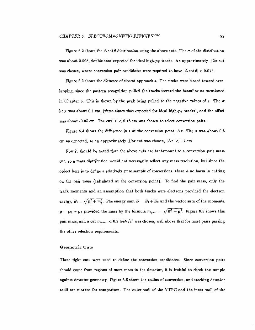
CHAPTER 6. ELECTROMAGNETIC EFFICIENCY 92
Figure 6.2 shows the ~cot() distribution using the above cuts. The u of the distribution
was about 0.008, double that expected for ideal high-PT tracks. An approximately ±2u cut
was chosen, where conversion pair candidates were required to have \~cot 9\ < 0.015.
Figure 6.3 shows the distance of closest approach s. The circles were biased toward over-
lapping, since the pattern recognition pulled the tracks toward the beamline as mentioned
in Chapter 5. This is shown by the peak being pulled to the negative values of s. The u
here was about 0.1 em, (three times that expected for ideal high-PT tracks), and the offset
was about -0.05 em. The cut \s\ < 0.16 em was chosen to select conversion pairs.
Figure 6.4 shows the difference in z at the conversion point, ~z. The u was about 0.5
em as expected, so an approximately ±2u cut was chosen, \~z\ < 1.1 em.
Now it should be noted that the above cuts are tantamount to a conversion pair mass
cut, so a mass distribution would not necessarily reflect any mass resolution, but since the
object here is to define a relatively pure sample of conversions, there is no harm in cutting
on the pair mass (calculated at the conversion point). To find the pair mass, only the
track momenta and an assumption that both tracks were electrons provided the electron
energy, E; = VPr + m~. The energy sum E = E1 + E 2 and the vector sum of the momenta
p = Pl + P2 provided the mass by the formula Tnpair = y'E2 - p 2 • Figure 6.5 shows this
pair mass, and a cut Tnpair < 0.2 GeV /c2 was chosen, well above that for most pairs passing
the other selection requirements.
Geometric Cuts
These tight cuts were used to define the conversion candidates. Since conversion paus
should come from regions of more mass in the detector, it is fruitful to check the sample
against detector geometry. Figure 6.6 shows the radius of conversion, and tracking detector
radii are marked for comparison. The outer wall of the VTPC and the inner wall of the
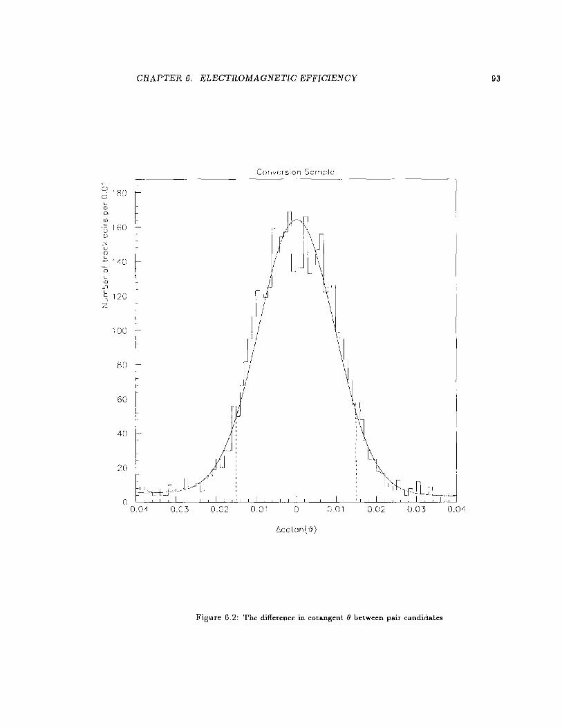
CHAPTER 6. ELECTROMAGNETIC EFFICIENCY
-'-<_; 0
_.':, 1 L[) ~
0
t 1 '){', ..J LU
/-
100
r
I r so r
~:t-=:P-L-/ L r f1_c/J
0 I I I I I ' I I I I ! I I
0.04 -0.03 -0.02
Conversion Sc rn :->lc
I I I I I I 1 I I I I I I
0.01 0 C.01
6colon(11)
0.02 0.03
Figure 6.2: The difference in cotangent (} between pair candidates
93
0.04
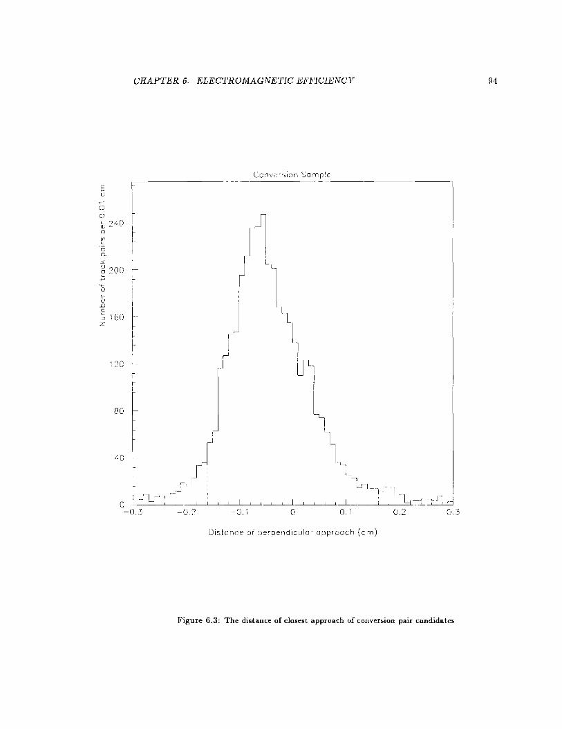
CHAPTER 6. ELECTROMAGNETIC EFFICIENCY
E l)
CJ (]
G.: 240 (l
~ 0 0~
"' 2 200 l_
0 [ '-QJ
I .D E 16Cl :J z
120
80
40
-0.3
/ .-.I :
-0./
Conve r:; ion Sam p' c
l I ~
" II I Lfl1
I
- Ci. I 0
l~ l~
0.1
Distance of perpendicular approach (em)
0.2 0.3
Figure 6.3: The distance of closest approach of conversion pair candidates
94
CHAPTER 6. ELECTROMAGNETIC EFFICIENCY
E u .,..- 240 ·-c:i L-OJ I 0. ({) r L- I_ "6 I 0. 200 ~ I u I 0 L-..., 0 L-OJ
.D 160 E :::J z
120
8Q I L
I 1,
I
40
Conversion Sample
J
rrll I~
\ or L ..1_1 _L__j_l _L_I _j_I_-'=!::!:O=!....LL_L._.L...J__LI _j: I__LI _j!__l__j!L..l_l _j!L..l_! _jiL__jiL..l__L_I ~..l_L.r..::'~"='---"1------'=L..l_l _oh_tt=J:l..l...! -'"'~'
-4 -3 -2 -1 0 1 2 3 4
f:::.z at perpendicular approach (em)
Figure 6.4: The z difference between conversion pair candidate tracks
95
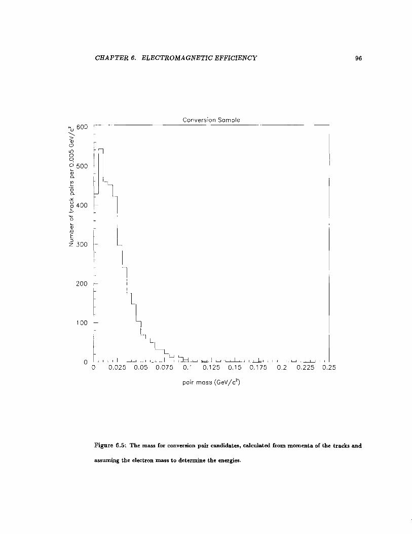
CHAPTER 6. ELECTROMAGNETIC EFFICIENCY 96
Conversion Sample "'u 600 -"-> OJ Cl L[) 0 q 0 500 .... OJ Q_
UJ .... '6 Q_
~
g 400 .... ....., .... 0 "-OJ
.D E :J z 300
200
100
0
,.II -~
l
l I
\I i ~ l I I I I ~!::=:±=! I I t::::::i I I I I I~ I I I I I I J I I I I I
0 0.025 0.05 0.075 0.1 0.125 0.15 0.175 0.2 0.225 0.25
pair mass (GeV/c2)
Figure 6.5: The mass for conversion pair candidates, calculated from momenta of the tracks and
assuming the electron mass to determine the energies.
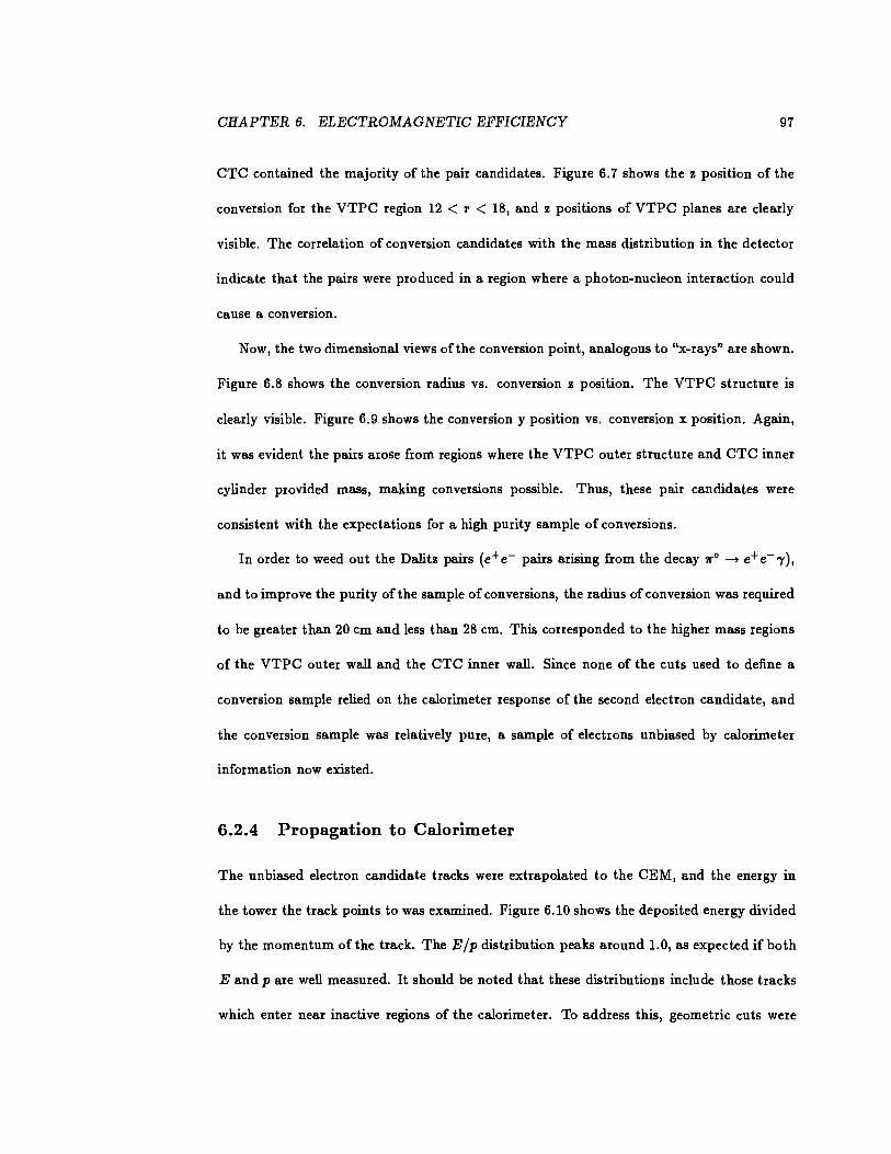
CHAPTER 6. ELECTROMAGNETIC EFFICIENCY 97
CTC contained the majority of the pair candidates. Figure 6. 7 shows the z position of the
conversion for the VTPC region 12 < r < 18, and z positions of VTPC planes are clearly
visible. The correlation of conversion candidates with the mass distribution in the detector
indicate that the pairs were produced in a region where a photon-nucleon interaction could
cause a conversiOn.
Now, the two dimensional views of the conversion point, analogous to "x-rays" are shown.
Figure 6.8 shows the conversion radius vs. conversion z position. The VTPC structure is
clearly visible. Figure 6.9 shows the conversion y position vs. conversion x position. Again,
it was evident the pairs arose from regions where the VTPC outer structure and CTC inner
cylinder provided mass, making conversions possible. Thus, these pair candidates were
consistent with the expectations for a high purity sample of conversions.
In order to weed out the Dalitz pairs (e+e- pairs arising from the decay 1!'0 --+ e+e--y),
and to improve the purity of the sample of conversions, the radius of conversion was required
to be greater than 20 em and less than 28 em. This corresponded to the higher mass regions
of the VTPC outer wall and the CTC inner wall. Since none of the cuts used to define a
conversion sample relied on the calorimeter response of the second electron candidate, and
the conversion sample was relatively pure, a sample of electrons unbiased by calorimeter
information now existed.
6.2.4 Propagation to Calorimeter
The unbiased electron candidate tracks were extrapolated to the CEM, and the energy in
the tower the track points to was examined. Figure 6.10 shows the deposited energy divided
by the momentum of the track. The E fp distribution peaks around 1.0, as expected if both
E and pare well measured. It should be noted that these distributions include those tracks
which enter near inactive regions of the calorimeter. To address this, geometric cuts were
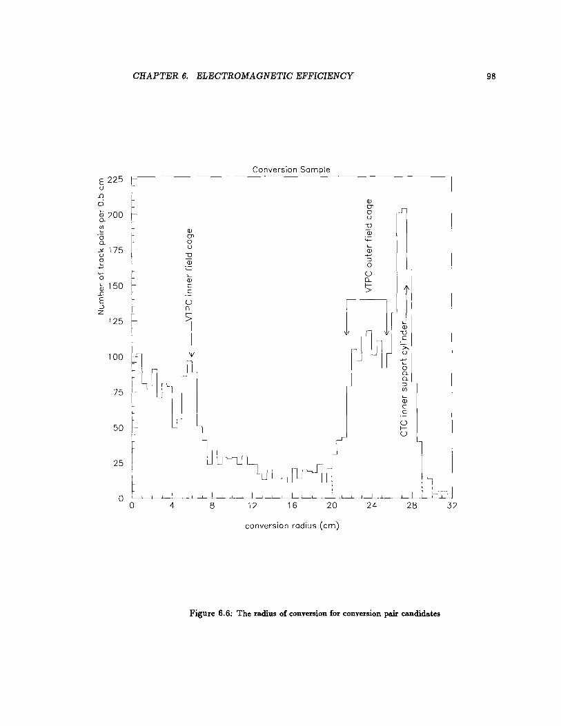
E 225 u
L[)
0
~ 200 0.. rn '--
"6 0..
..:,(. 175 u 0 '--....,
.,_ 0 ~ 150
.D E ::J z
125
100
CHAPTER 6. ELECTROMAGNETIC EFFICIENCY
0 4
Q) 0"1 0 u -o
'-Q) c c
8
Conversion Sample --------------------.
12 16 20
conversion radius (em)
Q) 0"1 0 u -o Qi
I I
24
L... Q) c c u r-u
ll ' L--, j
I f I I I -
28 32
Figure 6.6: The radius of conversion for conversion pair candidates
98
CHAPTER 6. ELECTROMAGNETIC EFFICIENCY
E 90
~ .__ (lJ
D. 80 -
0 D.
0 t 0 I
-100
Conversion Sample ---------------------
\! I VTPCmo~ \V pos;t;o,"J """ I
60 £11 ID
80 I I 100
conversion z (em), VTPC region
Figure 6. 7: The conversion z coordinate for conversion pair candidates
99
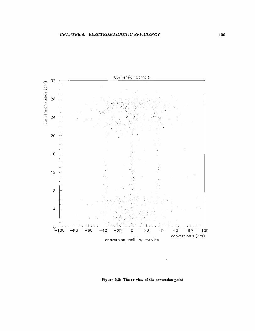
CHAPTER 6. ELECTROMAGNETIC EFFICIENCY 100
,--.- 32 Conversion Sample
E ()
-..._./
Ul ::J
f -o 28 0 . ~ L
c ... 0 ·• 'iii L QJ
~ > 24 .. ~ '
c 0 () ·.'
20 I I I
16
12
8
4
r
0 ,_Li_L,J_..._i_.!_L..L_li-L...L..L-'-'--'-'-'-..L..L--'-'L...L..J..C.J'--L-'--.L-->......L....L.:.L_L..L...L:_I-L...J__J.__L_J_J__J_JL...J._...L...l-<--J
-100 -80 -60 -40 -20 0 20 40 60 80 100
conversion position, r-z view conversion z (em)
Figure 6.8: The rz view of the conversion point
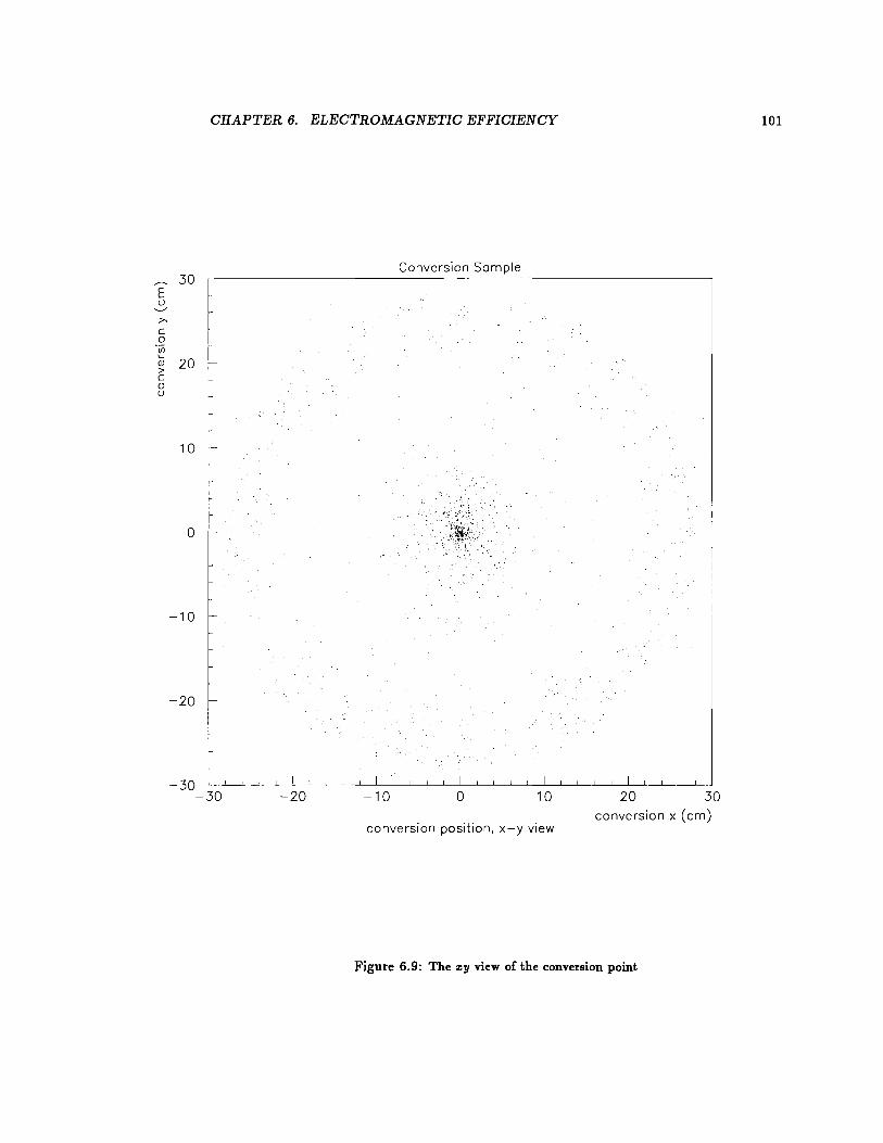
CHAPTER 6. ELECTROMAGNETIC EFFICIENCY 101
Conversion Sample ,..---.. 30
t E u
'-.../
;>, I c I 0 I 'iii ,-1.-
20 Q) > c 0 u
10 L
0
-10
-20
-30 -30 -20 -10 0 10 20 30
conversion position, x-y view conversion x (em)
Figure 6.9: The zy view of the conversion point
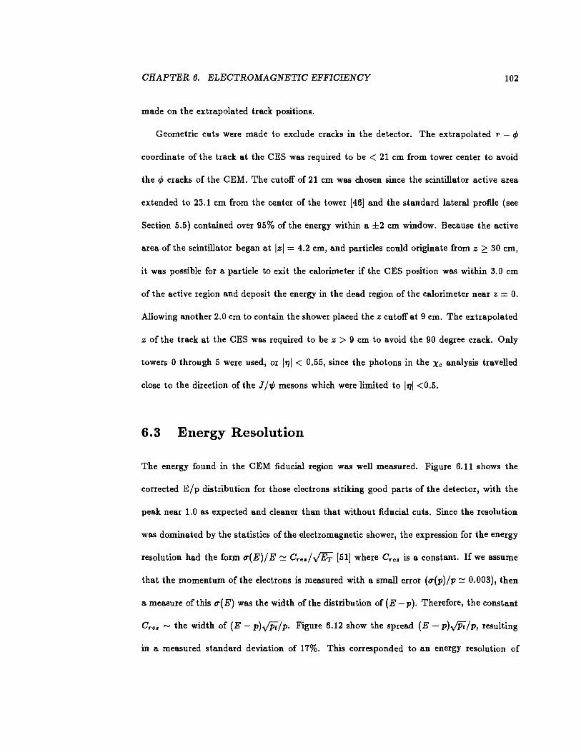
CHAPTER 6. ELECTROMAGNETIC EFFICIENCY 102
made on the extrapolated track positions.
Geometric cuts were made to exclude cracks in the detector. The extrapolated r - ¢
coordinate of the track at the CES was required to be < 21 em from tower center to avoid
the ¢ cracks of the CEM. The cutoff of 21 em was chosen since the scintillator active area
extended to 23.1 em from the center of the tower [46] and the standard lateral profile {see
Section 5.5) contained over 95% of the energy within a ±2 em window. Because the active
area of the scintillator began at lzl = 4.2 em, and particles could originate from z 2:: 30 em,
it was possible for a particle to exit the calorimeter if the CES position was within 3.0 em
of the active region and deposit the energy in the dead region of the calorimeter near z = 0.
Allowing another 2.0 em to contain the shower placed the z cutoff at 9 em. The extrapolated
z of the track at the CES was required to be z > 9 em to avoid the 90 degree crack. Only
towers 0 through 5 were used, or 1711 < 0.55, since the photons in the Xc analysis travelled
close to the direction of the J /.,P mesons which were limited to 1711 <0.5.
6.3 Energy Resolution
The energy found in the CEM fiducial region was well measured. Figure 6.11 shows the
corrected E/p distribution for those electrons striking good parts of the detector, with the
peak near 1.0 as expected and cleaner than that without fiducial cuts. Since the resolution
was dominated by the statistics of the electromagnetic shower, the expression for the energy
resolution had the form u(E)/E ~ Cre•/JET [51] where Cre• is a constant. If we assume
that the momentum of the electrons is measured with a small error (u(p)/P ~ 0.003), then
a measure of this u(E) was the width of the distribution of {E-p). Therefore, the constant
Cre• ~ the width of (E- p).;pifp. Figure 6.12 show the spread {E- p).jPt/p, resulting
in a measured standard deviation of 17%. This corresponded to an energy resolution of
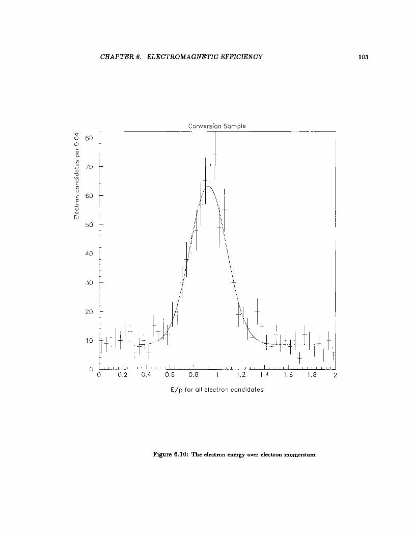
CHAPTER 6. ELECTROMAGNETIC EFFICIENCY
Conversion Sample
~ 80 -0
I
50 -
40 -
30 -
t 20 l
~ · , 11 ~ t; J 10 ~+I h ,ill/
~it J . 'lll ,-'H++ ltA 1
D 0 0.2 0.4 0.6
' . ' 0.8
I ic[' 1 t I I I 1.2 1.4 1.6 1.8
E/p for all electron candidates
Figure 6.10: The electron energy over electron momentum
2
103
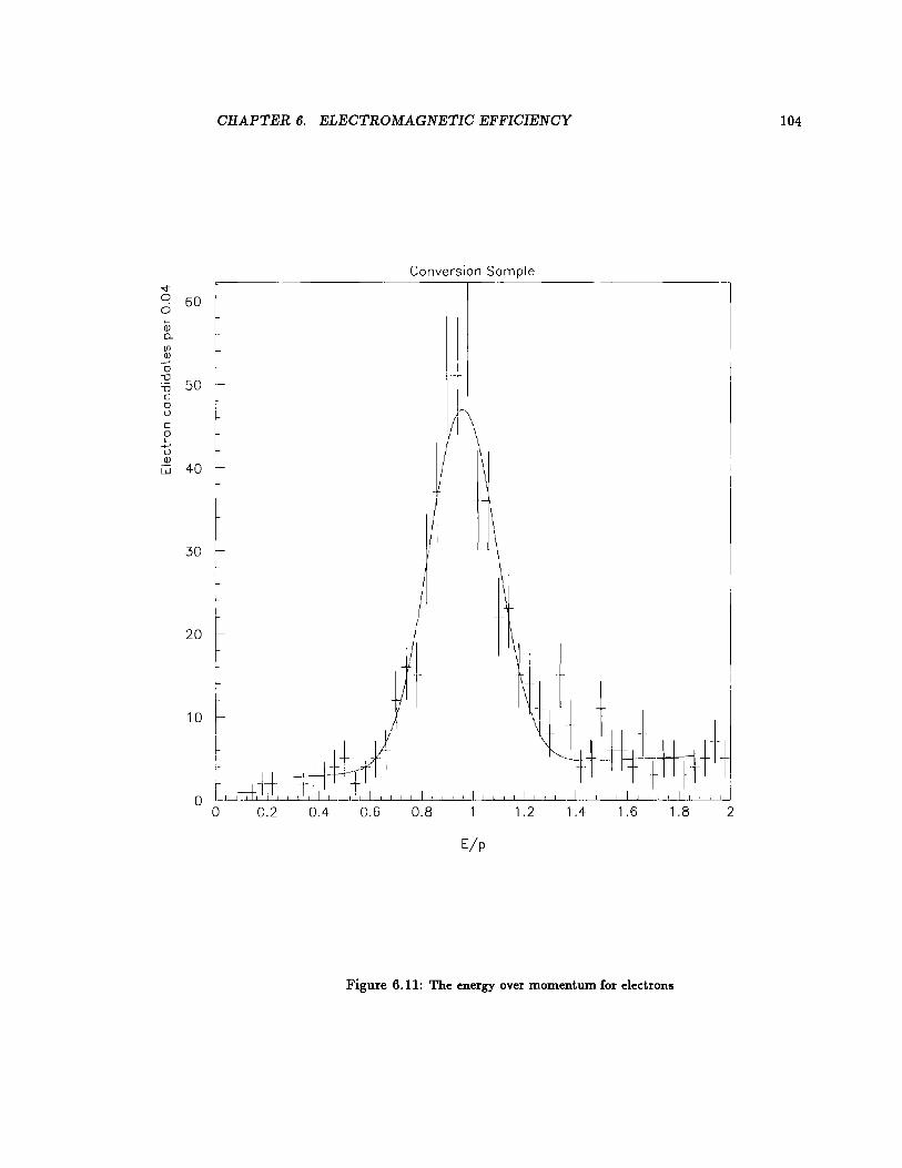
CHAPTER 6. ELECTROMAGNETIC EFFICIENCY 104
Conversion Sample
E/p
Figure 6.11: The energy over momentum for electrons
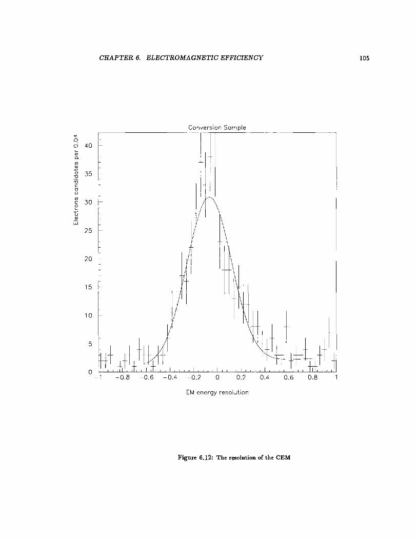
CHAPTER 6. ELECTROMAGNETIC EFFICIENCY
Conversion Sample ~------------------
~ 30 L 0 I
~ I u a.> w
25
20 '
15 ,L
10
5
-0.8 -0.6 -0.4 -0.2 0 0.2
EM energy resolution
0.4 0.6
Figure 6.12: The resolution of the CEM
105
0.8

CHAPTER 6. ELECTROMAGNETIC EFFICIENCY 106
u(E)/E := 17%/../ET.
6.4 Position Resolution
The position resolution of the CES clustering was found by comparing the cluster position to
where the electron track aimed. Figure 6.13 shows the track match to CES cluster positions
in both the r - ¢ and z views. Fits to these distributions show that the position resolution
for CES clusters arising from these electrons was around 0.8 em in the r - ¢ direction, and
1.0 em in the z direction.
6.5 Electron Efficiency
The electron efficiency was determined by the number of identified electrons which pass
the electromagnetic cluster finding algorithm. The default clustering (outlined in Section
5.5) was used. Figure 6.14 shows the momentum of all tracks passing the cuts (including
geometric), as well as the momentum distribution of those tracks which had a cluster with
energy in both views. The electron efficiency was measured from the percentage of the
electron candidates that produced CES clusters. Figure 6.15 shows the ratio of the two,
which is the CES efficiency as a function of electron momentum.
The efficiency of the algorithm must also include the effects of energy cuts, since the
energy resolution of the detector would affect the acceptance of energy requirements. Fig-
ure 6.16 shows the efficiency if, in addition to energy in both views of the cluster, an EM
energy of 1 Ge V was required. This was the efficiency (as a function of electron momentum)
of the actual electromagnetic shower selection for this analysis.
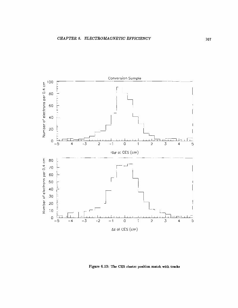
CHAPTER 6. ELECTROMAGNETIC EFFICIENCY
Conversion Sample E 100 ----
u <:1" ci 80 ..._ Q) Q_
(/) c 60 0 ..._
->-' u Q)
OJ 40 i-.,__ 0 ..._ Q)
_o 20 E r :::J z 0 l.ccrr~l •• ,,l I I I I I
-5 -4 -3
E 80 l u <:t: 70 0 -..._ .~
Q) 60 r Q_
(/) c 50 0 ..._
->-' -u 40 ~ r OJ
f 4-- 30 0 '--Q) 20 _o
E -:::J 10 -z
b~J-.L 0 -5 -4 -3
-2
-2
-1 0
rb.rp at CES (em)
~-
1
l \~ I
1,, ""'I"~ I I I I
-1 0 2 3 4 5
t:.z at CES (em)
Figure 6.13: The CES cluster position match with tracks
107
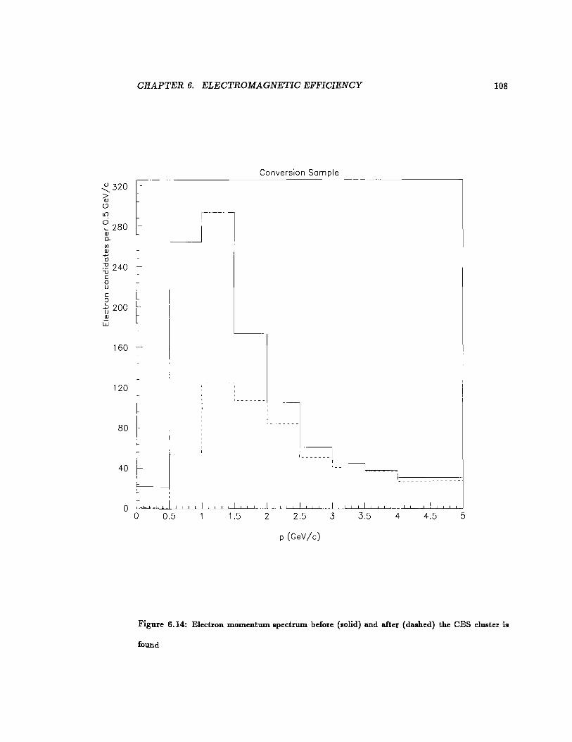
CHAPTER 6. ELECTROMAGNETIC EFFICIENCY
<320 ~ <..? L[)
~ 280 Q) D. If) Q) .....
1- _j 0 ~ 240 -o c 0 u
1-
c l 0 ~ 200 i ~ LL w
I 160
120
80 -
40 I
c-~-
0 ~~. 0 0.5
Conversion Sample
' ·---------~
1.5 2 2.5 3 3.5 4
p (GeV/c)
108
4.5 5
Figure 6.14: Electron momentum spectrum before (solid) and after (dashed) the CES cluster is
found
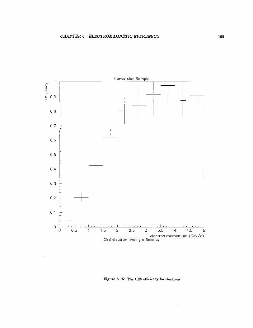
>-u c Q)
·u .;: 0.9 .,_. Q)
0.8
0.7
0.6
0.5
0.4
0.3
0.2
0.1
0
CHAPTER 6. ELECTROMAGNETIC EFFICIENCY
Conversion Sample ------------------------~ [ 2J I I ~ r-1-I_ '-
I ~
-+-
0 0.5
-[ I
1.5 2 2.5 3 3.5 4 4.5 5 electron momentum (GeV/c)
CES electron finding efficiency
Figure 6.15: The CES efficiency for electrons
109
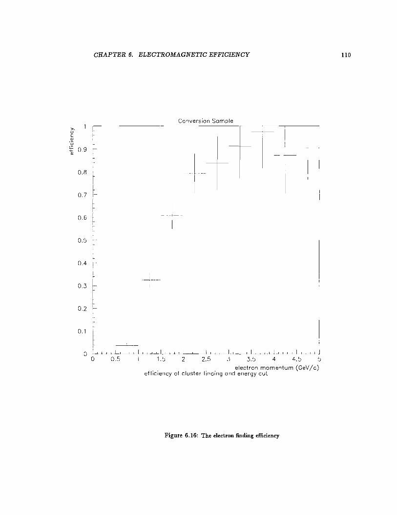
>-u c Q)
'() ~ 0.9 Qj
0.8
0.7
0.6
0.5
0.4
0.3
0.2
0.1
0
CHAPTER 6. ELECTROMAGNETIC EFFICIENCY
1-~
'
1-~
-
~
e.
[ I
f I 0 0.5
Conversion Sample
+ I
~-1
1.5 2 2.5 3 3.5 4 4.5 5 electron momentum (GeV/c)
efficiency of cluster finding and energy cut
Figure 6.16: The electron finding efficiency
110
CHAPTER 6. ELECTROMAGNETIC EFFICIENCY 111
6.6 CES Simulation
The photon efficiency was slightly different from the electron efficiency due to a difference in
longitudinal shower development. Electromagnetic showers produced by photons travelled
further into the CEM, allowing more of the low-energy shower to reach the CES than was the
case with electrons. To model the difference in efficiency arising from this fact, a GEANT
(version 3.14) simulation ofthe CES response for both electrons and photons was performed.
The GEANT simulations of electrons and photons in the CES were used to compare photon
response with electron response. The electron simulation did a reasonable job of predicting
the average pulseheight versus energy observed in the test beam electron runs, quantified
in References [52, 53, 54]. This simulation produced tables of charge deposition segmented
according to the CES geometry on an event by event basis. These events were then scaled
according to the strip chamber gain and put into a form that could be processed by the
strip chamber clustering code and clustered in the same way as the data was. The deviation
of channel energy due to noise was l the effective channel threshold and would contribute
negligibly to the efficiency, so was not included in the model.
6.6.1 Comparison of GEANT Electron to Data
Electron showers were simulated with the CDF calorimeter geometry. The simulated elec-
tron shower profiles could be directly compared to those for the electrons in the conversion
sample to ensure the showers were modelled correctly. First, a few distributions with widely
varying detector gains (relative 0.625,1.0,1.25) for GEANT electrons were compared with
data to test the efficacy of the GEANT simulation. These relative scales were to study the
effects of uncertainties in the modelling of the gas gain in the simulation. Figure 6.17 com-
pares the average wire cluster energy ofGEANT electrons with the average from conversion
CHAPTER 6. ELECTROMAGNETIC EFFICIENCY 112
electrons as a function of electron momentum. This figure shows that the actual gas gain in
the detector was bounded by the chamber gain assignments in the simulation. Figure 6.18
compares the average energy for all generated GEANT events found to have non-zero cluster
energy to the same average for the electron sample. This was the same as the previous plot
with the exception of excluding events where no cluster was found. Again, the chamber
gains used in the simulation resulted in similar energy response behavior to that observed
in the cluster energies in the electron data. The real test of the usefulness of the simulation
was how well it described the electron efficiency. Figure 6.19 compares the cluster finding
efficiency for the simulation to that for electron data. The fact that the efficiencies match
well shows the simulation did a good job at modelling electron shower development in CDF,
and could be relied upon for a parameterization of electromagnetic shower development.
6.6.2 Comparison in GEANT: Electron to Photon
The simulation was then used to find the difference in CES detection efficiency for photon
and electron showers. Figure 6.20 shows the GEANT ratio of efficiency for cluster finding
of photons compared to that of electrons. The several different detector gains tested gave
almost identical e± h response ratios. The electron to photon CES efficiency ratio differed
from unity by less than 17% for all detector gains used and for all particle energies greater
than 1.0 GeV, while the value of the ratio varied less than 3% for the different gains used.
The slightly higher photon efficiency was due to the fact that at energies around 1.0 GeV,
electron showers would be mostly included within the material before the CES, while photons
would convert around 0.8 radiation lengths after the beginning of the material, and could
reach into the CES more often.
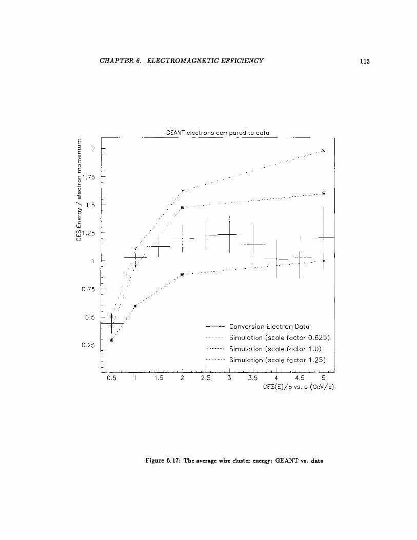
CHAPTER 6. ELECTROMAGNETIC EFFICIENCY
E :l
-+-' c Q)
E 0 E c 1.75 0 "---+-' u Q)
......__ 1.5 >, (J1 1...-Q) c w ~1.25 u
0.75
L
0.5 -
0.25
0:
0.5
GEANT electrons compared to data ------
)I(·
+·''.· '!(
1.5 2
I
+++I I I J-: J
2.5
~- - --- I I
Conversion Electron Data
Simulation (scale factor 0.625)
Simulation (scale factor 1.0)
Simulation (scale factor 1.25)
3 3.5 4 4.5 5 CES(E)/p vs. p (GeV/c)
Figure 6.17: The average wire cluster energy: GEANT vs. data
113
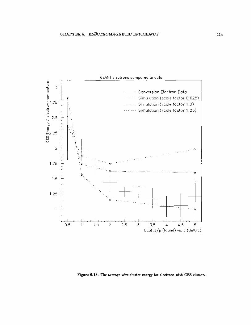
CHAPTER 6. ELECTROMAGNETIC EFFICIENCY
E 3 3 ~ c Q)
E 0 * E c2.75 - 1'·
0 \... ...- ' u Q)
Qi25 f-......__ >. (J"l
' \... Q) '\· .• I
t.52.25 ~ ,. ' .·.,
GEANT electrons compared to data -------------------,
Conversion Electron Data Simulation (scale factor 0.625) Simulation (scale factor 1.0) Simulation (scale factor 1.25)
~ ~ ·:-;.. I -~ ').
~~;-J_·. -2 ,._
1.75 f-
1.5 f-
\ --- -- - I -'*· ~---~ .. ::.- .. -.............................. __ * I -- ........................................... *
I
1.25 I
l~ 0~--+ I ~--
*'----
I , I ' I I I . I I I 0.5 1.5 2 2.5 3 3.5 4 4.5 5
CES(E)/p (found) vs. p (GeV/c)
Figure 6.18: The average wire cluster energy for electrons with CES clusters
114
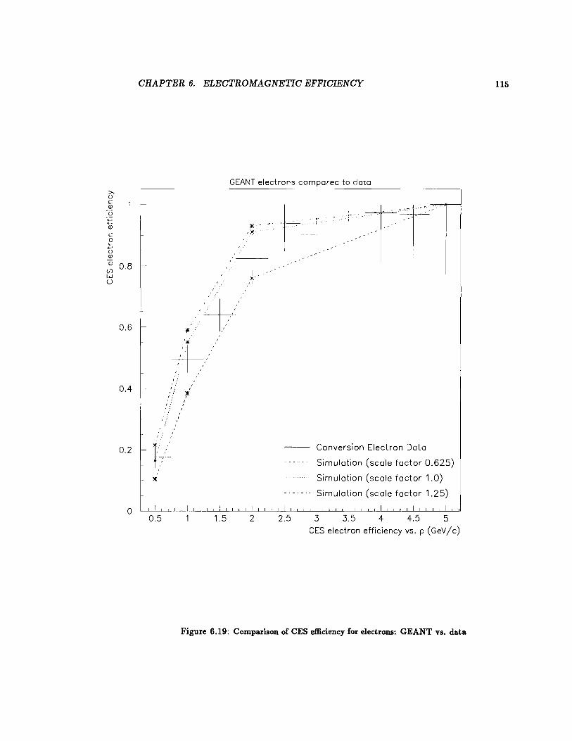
>. 0 c Q)
'() 4--
'iii c 0 L ..... 0 Q)
Q)
(/) w u
CHAPTER 6. ELECTROMAGNETIC EFFICIENCY
'--I
0.8
o.6 I
0.4
0.2 -
0
GEANT electrons compared to doto
+.· . ' '~
I ' . •
. I ...
'I(.··· '
+·i :' : .
,': I ... •,' I
1.' 1
,·,.: ~ ,,:
I
' ... / . '
.~ .... ¥ r··r·~
J
t.:~
Conversion Electron Data
Simulation (scale factor 0.625)
Simulation (scale factor 1.0)
Simulation (scale factor 1.25)
)1:
I -'--l I I I I I I I 0.5 1.5 2 2.5 3 3.5 4 4.5 5
CES electron efficiency vs. p (GeV/c)
Figure 6.19: Comparison of CES efficiency for electrons: GEANT vs. data
115
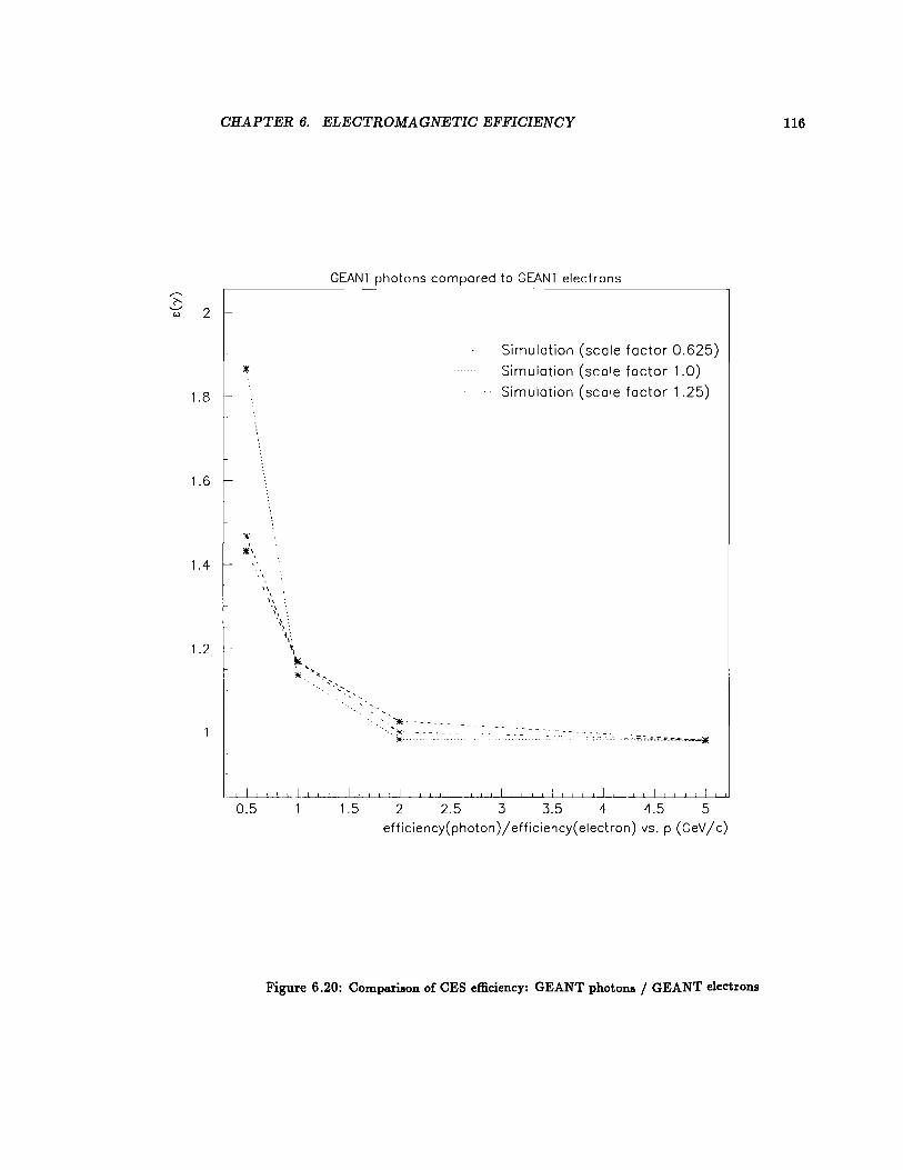
CHAPTER 6. ELECTROMAGNETIC EFFICIENCY
GEANT photons compared to GEANT electrons ~------
1.8 -
Simulation (scale factor 0.625) Simulation (scale factor 1.0) Simulation (scale factor 1.25)
1.6
1.4
1.2
,'' - ....... ''
··.)<--"""' ..
ft_L_L__C.._l__l_L,.L_L..._L.L-'-l.-'-----L..L--'-L____l_L..L_l_L--'-.L..L-L-L--'-.JL..J__J._l___L_jl_l__.Lj_,
0.5 1 1.5 2 2.5 3 3.5 4 4.5 5 efficiency(photon)/efficiency(electron) vs. p (GeV/c)
Figure 6.20: Comparison of CES efficiency: GEANT photons / GEANT electrons
116
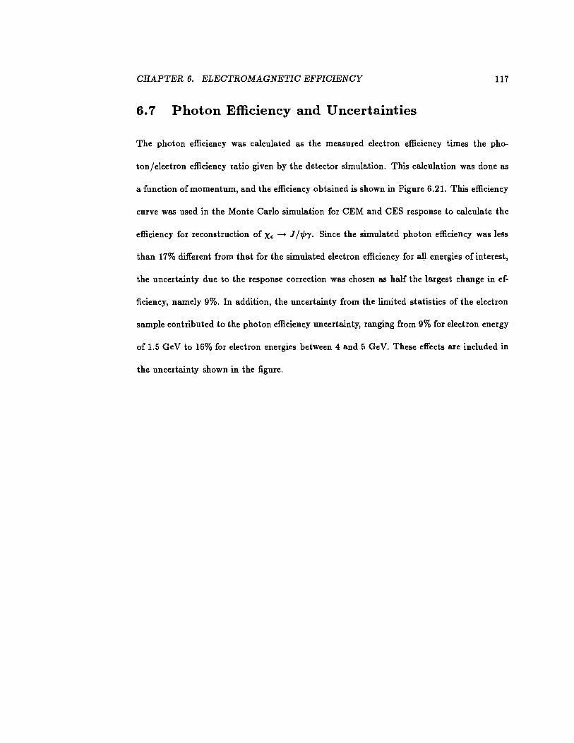
CHAPTER 6. ELECTROMAGNETIC EFFICIENCY 117
6. 7 Photon Efficiency and Uncertainties
The photon efficiency was calculated as the measured electron efficiency times the pho-
ton/electron efficiency ratio given by the detector simulation. This calculation was done as
a function of momentum, and the efficiency obtained is shown in Figure 6.21. This efficiency
curve was used in the Monte Carlo simulation for CEM and CES response to calculate the
efficiency for reconstruction of Xc --+ J / tP'Y. Since the simulated photon efficiency was less
than 17% different from that for the simulated electron efficiency for all energies of interest,
the uncertainty due to the response correction was chosen as half the largest change in ef-
ficiency, namely 9%. In addition, the uncertainty from the limited statistics of the electron
sample contributed to the photon efficiency uncertainty, ranging from 9% for electron energy
of 1.5 GeV to 16% for electron energies between 4 and 5 GeV. These effects are included in
the uncertainty shown in the figure.
CHAPTER 6. ELECTROMAGNETIC EFFICIENCY 118
Photon Efficiency - GEANT Corrected Electron Efficiency ---'------
~ .21 '
1 ~ I __ +
_l_ 0.8 tl 0.6
0.4 --+ 0.2
0 0.5 1.5 2 2.5 3 3.5 4 4.5 5
-y Efficiency vs. -y Energy (GeV)
Figure 6.21: The photon finding efficiency

Chapter 7
Acceptance Determination
Calculating the detector acceptance for a given type of event can be an extremely difficult
process. The actual detector geometry and response need to be applied to the kinematic
distributions expected for the events. This can involve integrations which are extremely
difficult to solve analytically. There are, however, ways of numerically evaluating complex
integrals. One is a method involving random numbers, called the Monte Carlo method.
The Monte Carlo method generates simulated physics events randomly within the energy
ranges allowed by a model of the physical process under investigation. These simulated
events have the same momenta spectra, rapidity spectra, and other quantities as the model
predicts for the actual process. The positions and energies can be used to determine the
efficiency for the observation of the process in question. The application of the Monte Carlo
method to the process Xc --+ J f1/ry is discussed in this chapter.
The Xc reconstruction efficiency can be factored into several terms: the geometric ac-
ceptance (a function of the muon and photon fiducial and kinematic cuts), the efficiency
of the J /..P selection requirements (which depends on the muon identification requirements,
119

CHAPTER 7. ACCEPTANCE DETERMINATION 120
the muon trigger efficiency, and the J /1/J reconstruction efficiency), and the efficiency of the
photon selection requirements. The simulation of the process and the determination of the
acceptance is examined by the following method.
• Monte Carlo Xc --+ J /1/Jr events were generated for each production mechanism, pro-
viding different hypotheses for the Xc PT and 1J spectra. These Monte Carlo generators
are outlined in Section 7.1.
• A detector simulation was applied to each generated sample, to find the acceptance
times efficiency for reconstructing Xc --+ J /1/Jr from each initial hypothesis. The
acceptance and efficiency will depend somewhat on the production hypothesis, as will
be shown in Section 7.2.
• The question as to which set of production hypotheses for the Monte Carlo samples
best simulated the actual is addressed in Section 7.3. This discussion will justify the
central value for acceptance times efficiency which will be used to calculate the true
number of events produced in the jip collisions.
7.1 Monte Carlo Generators
Two separate Monte Carlo programs generated the similated Xc --+ J / 1/Jr for the efficiency
studies. The first modelled direct Xc production, while the second simulated B meson
production and subsequent decay into Xc states. Both of these are described in this section.
CHAPTER 7. ACCEPTANCE DETERMINATION 121
7.1.1 Direct Xc Production
ISAJET: General Description
ISAJET is a Monte Carlo event generator for pp or pjj interactions at the high energies [55]
such as those produced at the Tevatron. It includes a perturbative QCD calculation of the
parton level hard scattering process, leading order QCD initial and final state radiation, and
some models for fragmentation of both the partons and the initial beams. The hard scat-
tering processes available within the standard ISAJET program have not to date included
quarkonia production, so a modification to the program to do this is described below.
ISACHI: Charmonia Generation
The modification of ISAJET for including the charmonia cross section calculation of Equa-
tion 2.4 was named ISACHI. It calculated the parton level cross sections for the process
gg -+ xcg for the angular momentum states J =0,1,2. These parton level cross sections
were calculated from Equation 2.2 with the functional forms as outlined in Reference [18].
The cross sections were then multiplied by the branching ratio for the Xc state to decay
into J /1/Jr. These decays were the only ones allowed for Xc mesons. This had the effect of
properly scaling the relative number of J /1/Jr from each angular momentum state.
The value of a, was calculated with a number of different expressions for Q2 , to provide
an estimate of the systematic uncertainty on the acceptance calculation due to the uncer-
tainty in the scale. The central value was chosen from the Monte Carlo with the momentum
transfer proportional to the transverse mass Q2 = (p}+m~)/4. For the purposes ofPT slope
and acceptance determination, the constant had no effect. A stiffer spectrum (with more
events in the higher PT regions) was obtained from Q2 = m~. To examine softer spectra,
one more function for Q2 , for which there was no physical basis except that it provided a
CHAPTER 7. ACCEPTANCE DETERMINATION 122
steeply falling spectrum, were used to generate events as well. The funcional form for this
was Q2 = (m~ + p~fmx)/6.
Resultant J /1/J and Xc PT Distributions
The kinematics for the simulated events with different forms for a. are observably different.
The Xc PT distributions from each Q2 is shown in Figure 7.1. The J /1/J distributions from
each are shown in Figure 7.2. In these Figures the difference in slope of the PT spectrum
from varying Q2 is apparent. Simple exponentials do not fit well to the spectra, so a single
number would not quantify the range, but the difference in the acceptance and overall
efficiency for each is discussed in Section 7.2.
7.1.2 B Generation
To determine the efficiency for detecting Xc mesons coming from B decay, a Monte Carlo
program generated B mesons which decayed into charmonia [56], B--+ xcX. This program
modelled b-quark production according to the Nason, Dawson, Ellis order-a~ calculation [23]
outlined in Section 2.2 providing the PT and 11 spectrum of the b-quark.
B mesons were generated with the relative fractions outlined in Equation 2. 7, which
were
(7.1)
while Be mesons and b-baryons where ignored. A Peterson E parameter of 0.006 was used,
defined in Equation 2.6, along with a b-quark mass of 5.0 GeV /c2 •
The B mesons were then decayed into two body states containing Xcl mesons. Since
only B --+ XclX decays have been found [26], the other angular momentum states were
not generated. The CLEO 90% upper confidence level limit on the B --+ Xc 2 X branching
fraction is 0.4% [26], while the combined CLEO and ARGUS results for the branching
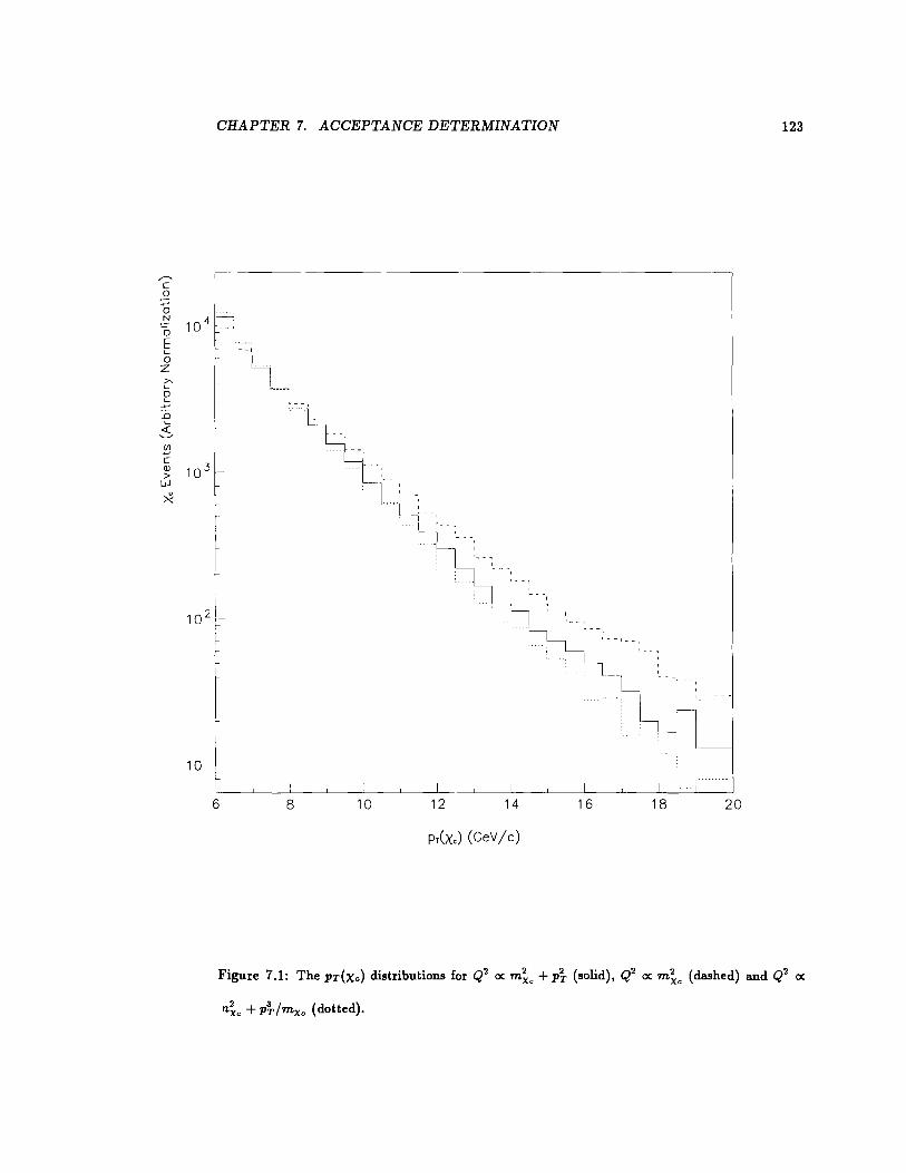
r---c: 0
CHAPTER 7. ACCEPTANCE DETERMINATION
,-----~---- ~--------------------,
10'1-
6 8
~l: .. - L .. :---~--~ '
10
' __ .. ' •--, .
-- -.
. L['~.
.. --~ .
12 14
Pr(Xc) ( GeV /C)
16 18 20
123
Figure 7.1: The PT(Xc) distributions for Q2 oc: m~c + p} (solid), Q2 oc: m~c (dashed) and Q2 oc:
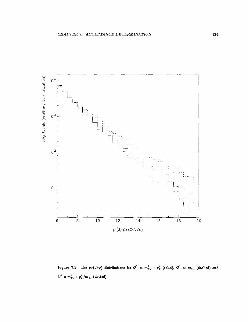
CHAPTER 7. ACCEPTANCE DETERMINATION 124
l
l --- : .. , __ , ·· .... _.-·h '-·. . . i
Lclj 10
6 8 10 12 14 16 18 20
Pr(J/1/1) (GeV /c)
Figure 7.2: The PT(JN) distributions for Q2 ex m;c + p~ (solid), Q2 (dashed) and
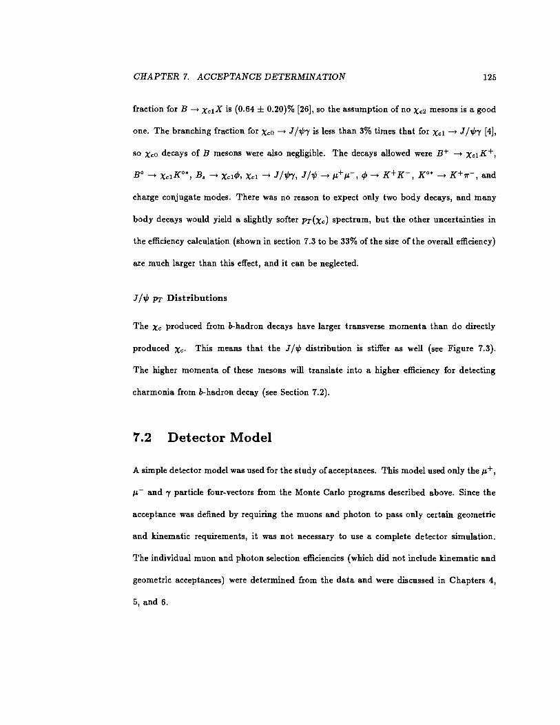
CHAPTER 7. ACCEPTANCE DETERMINATION 125
fraction forB --+ XclX is (0.64 ± 0.20)% [26], so the assumption of no xc2 mesons is a good
one. The branching fraction for Xco --+ J /1/J'Y is less than 3% times that for Xcl --+ J /1/J'Y [4],
so Xco decays of B mesons were also negligible. The decays allowed were B+ --+ xc1K+,
B 0 --+ Xc1K0 *, B, --+ XclrP, Xcl --+ J /1/J'Y, J /1/J --+ J.L+ J.L-, r/J--+ x+ x-, K 0 * --+ K+11'-, and
charge conjugate modes. There was no reason to expect only two body decays, and many
body decays would yield a slightly softer PT(Xc) spectrum, but the other uncertainties in
the efficiency calculation (shown in section 7.3 to be 33% of the size oft he overall efficiency)
are much larger than this effect, and it can be neglected.
J N PT Distributions
The Xc produced from b-hadron decays have larger transverse momenta than do directly
produced Xc· This means that the J /.,P distribution is stiffer as well (see Figure 7.3).
The higher momenta of these mesons will translate into a higher efficiency for detecting
charmonia from b-hadron decay (see Section 7.2).
7.2 Detector Model
A simple detector model was used for the study of acceptances. This model used only the J.L+,
J.L- and 'Y particle four-vectors from the Monte Carlo programs described above. Since the
acceptance was defined by requiring the muons and photon to pass only certain geometric
and kinematic requirements, it was not necessary to use a complete detector simulation.
The individual muon and photon selection efficiencies (which did not include kinematic and
geometric acceptances) were determined from the data and were discussed in Chapters 4,
5, and 6.
CHAPTER 7. ACCEPTANCE DETERMINATION 126
r-- , o4l_ c 0
:;:; ~ 0 N -· 0
~ E L 0 z >. L 0 L
-<-' :0
1 o3 L <(
i ' ' ---
"'-' I--' (/)
-<-' I : c Q) > w ?-'-.. ~ ' J I __ ,--,
'
102
10
6 8 10 12 14 16 18 20
Pr(J/1/f) (GeV/c)
Figure 7.3: The PT(JN) distributions for direct production (solid) and B decay (dashed).
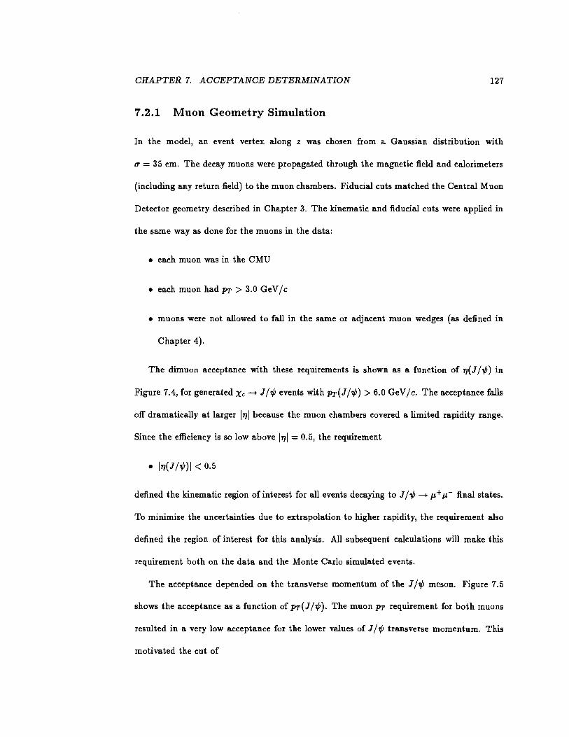
CHAPTER 7. ACCEPTANCE DETERMINATION 127
7.2.1 Muon Geometry Simulation
In the model, an event vertex along z was chosen from a Gaussian distribution with
u = 35 em. The decay muons were propagated through the magnetic field and calorimeters
(including any return field) to the muon chambers. Fiducial cuts matched the Central Muon
Detector geometry described in Chapter 3. The kinematic and fiducial cuts were applied in
the same way as done for the muons in the data:
• each muon was in the CMU
• each muon had PT > 3.0 GeV /c
• muons were not allowed to fall in the same or adjacent muon wedges (as defined in
Chapter 4).
The dimuon acceptance with these requirements is shown as a function of TJ(J / 1/J) in
Figure 7.4, for generated Xc -+ J /1/J events with PT( J N) > 6.0 GeV /c. The acceptance falls
off dramatically at larger 1111 because the muon chambers covered a limited rapidity range.
Since the efficiency is so low above 1111 = 0.5, the requirement
• I11(J N)l < o.5
defined the kinematic region of interest for all events decaying to J /1/J-+ J.L+ J.L- final states.
To minimize the uncertainties due to extrapolation to higher rapidity, the requirement also
defined the region of interest for this analysis. All subsequent calculations will make this
requirement both on the data and the Monte Carlo simulated events.
The acceptance depended on the transverse momentum of the J /1/J meson. Figure 7.5
shows the acceptance as a function of PT ( J / 1/J). The muon PT requirement for both muons
resulted in a very low acceptance for the lower values of J / 1/J transverse momentum. This
motivated the cut of
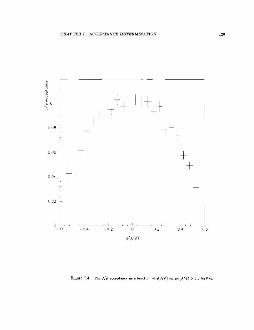
CHAPTER 7. ACCEPTANCE DETERMINATION
Q) l) c: 0 ...... Q_ Q) l) l) <( ? 0.1 ......... -:>
0.08
0.06 -
0.04
0.02
I T
+
I +_i ; + 1- +I + 1-
[- I -~
'Y/(J/1/1)
-+ + +
+
Figure 7.4: The JN acceptance as a function of 71(JN) for PT(JN) > 6.0 GeV Jc.
128
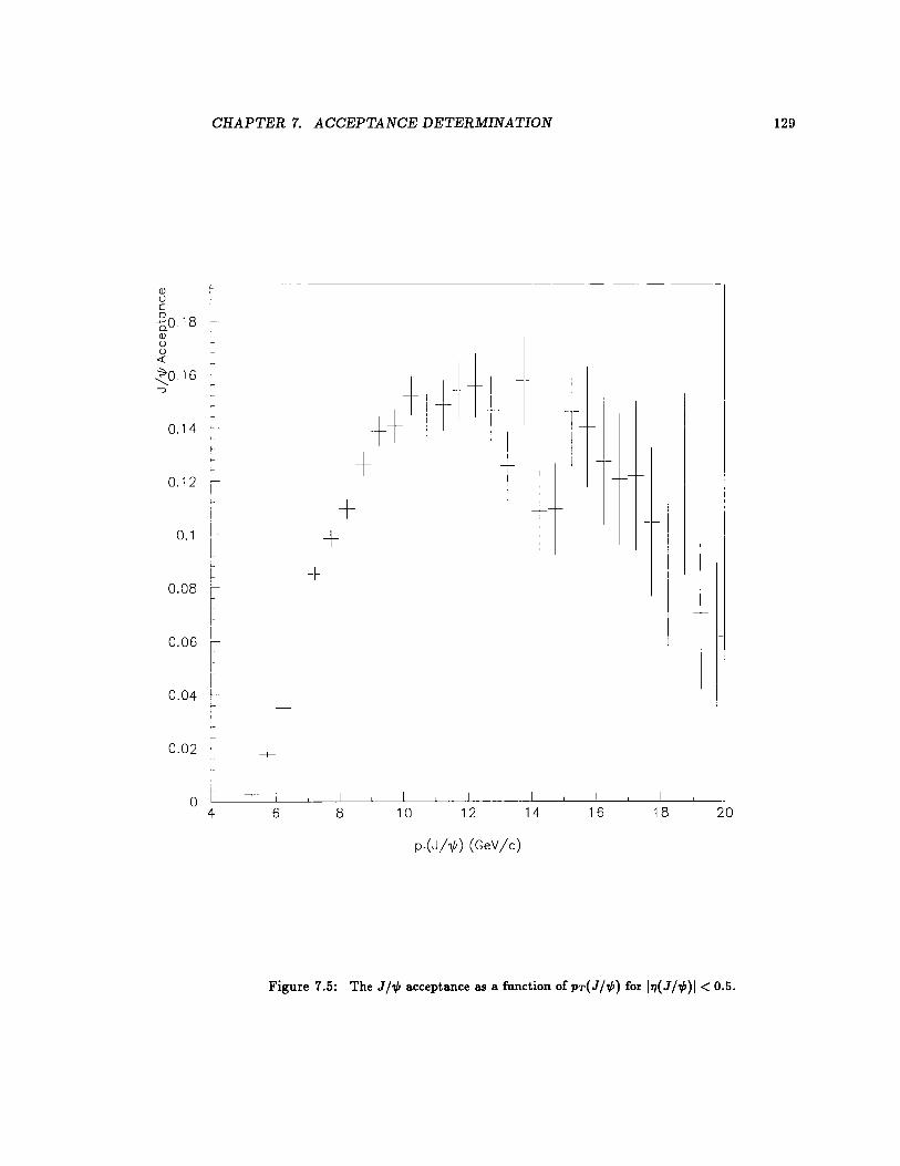
CHAPTER 7. ACCEPTANCE DETERMINATION 129
ClJ u c o .8 o_O ! -ClJ
t u u
tl++tlh <{
:to 16 c--,
' r 1-
0.14 i-
+ 0.12
+ j -
I 0.1 + I
+ I 0.08
0.06
0.04 -+-t
0.02 -+-
0 r- I 4 6 8 10 12 14 16 18 20
Pr(J/1/1) (GeV/c)
Figure 7.5: The JN acceptance as a function of PT(JN) for I11(JN)I < 0.5.
CHAPTER 7. ACCEPTANCE DETERMINATION 130
Process Acceptance
B--+ XcX (9.27 ± 0.17)%
Direct Xc Q2 -m2 - X (8.83 ± 0.18)%
Q 2 ex m~ + p} (7.74 ± 0.11)%
Q 2 ex m~ + P~lmx (7.48 ± 0.18)%
Table 7.1: The geometric and kinematic acceptance in the region PT(1 1'1/1) > 6.0 GeV lc and
111(1 1'1/1)1 < 0.5 for various simulated Xc--+ 1 N'Y event samples.
• PT(1 N) > 6.0 GeV lc
which defined the region of interest for 11'1/J production at CDF. All calculations will make
this requirement for both the data and simulated events. All conclusions and simulations
will be quoted for the kinematic range PT(1 N) > 6.0 GeV lc and 117(1 /'1/J)I < 0.5. The
efficiency also began to fall off at higher values of PT ( 1 I '1/;) since very energetic 1 I '1/; mesons
were more likely to have the ll+ and,.,- fall into adjacent muon wedges.
Since the acceptance is PT dependent, 1 1'1/1 production mechanisms with different PT
spectra had different acceptances. The acceptances, defined by all the above cuts for each of
the simulated Xc samples are summarized in Table 7.1. The uncertainties arise from Monte
Carlo statistics.
7.2.2 Muon Trigger Simulation
To simulate the trigger efficiency more fully, a paramaterization of the level one trigger was
used which relied on an understanding of the effects of multiple scattering on the muons
traversing the detector (see Chapter 8). To do this, the muons were assigned a track stub
slope in the CMU region depending on the PT· As discussed for the real data in Chapter 4,
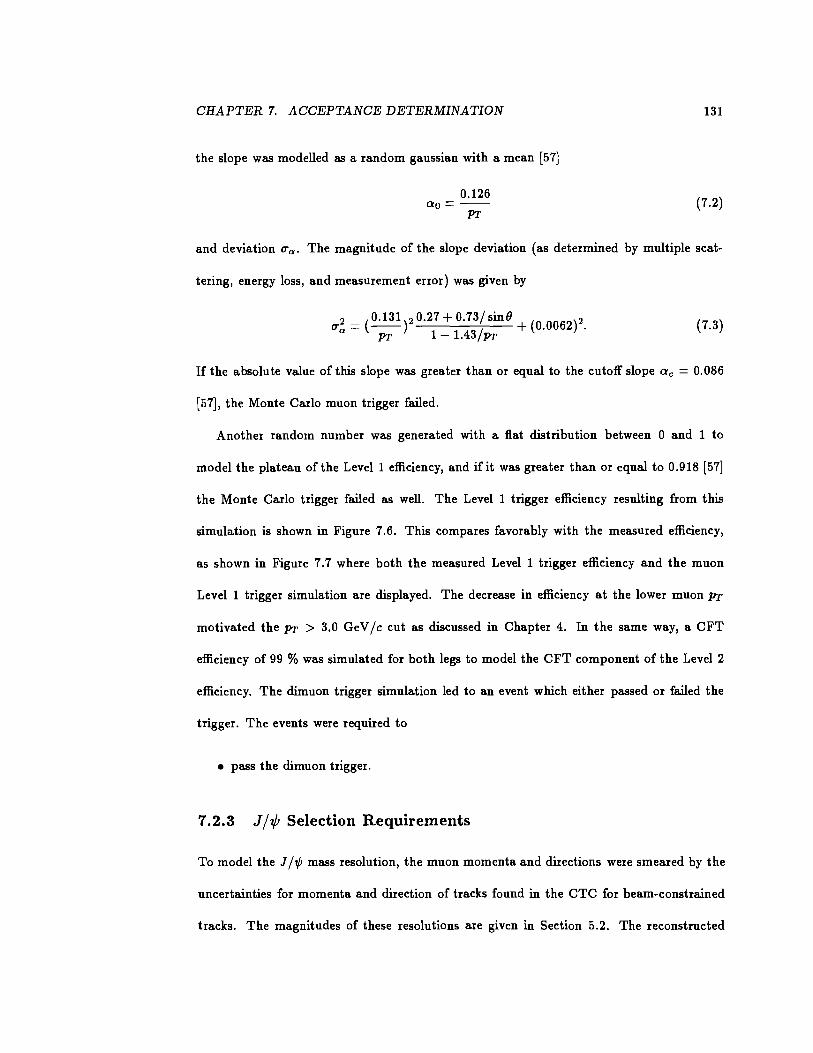
CHAPTER 7. ACCEPTANCE DETERMINATION 131
the slope was modelled as a random gaussian with a mean [57]
0.126 ao=--
PT (7.2)
and deviation u 0 • The magnitude of the slope deviation (as determined by multiple scat-
tering, energy loss, and measurement error) was given by
2 _(0.131) 2 0.27+0.73/sinO ( )2 Ua- -- 3/ + 0.0062 .
PT 1- 1.4 PT (7.3)
If the absolute value of this slope was greater than or equal to the cutoff slope Oc = 0.086
[57], the Monte Carlo muon trigger failed.
Another random number was generated with a fiat distribution between 0 and 1 to
model the plateau of the Level 1 efficiency, and if it was greater than or equal to 0.918 [57]
the Monte Carlo trigger failed as well. The Level 1 trigger efficiency resulting from this
simulation is shown in Figure 7.6. This compares favorably with the measured efficiency,
as shown in Figure 7.7 where both the measured Level 1 trigger efficiency and the muon
Level 1 trigger simulation are displayed. The decrease in efficiency at the lower muon PT
motivated the PT > 3.0 GeV jc cut as discussed in Chapter 4. In the same way, a CFT
efficiency of 99 % was simulated for both legs to model the CFT component of the Level 2
efficiency. The dimuon trigger simulation led to an event which either passed or failed the
trigger. The events were required to
• pass the dimuon trigger.
7.2.3 Jj¢ Selection Requirements
To model the J j,P mass resolution, the muon momenta and directions were smeared by the
uncertainties for momenta and direction of tracks found in the CTC for beam-constrained
tracks. The magnitudes of these resolutions are given in Section 5.2. The reconstructed
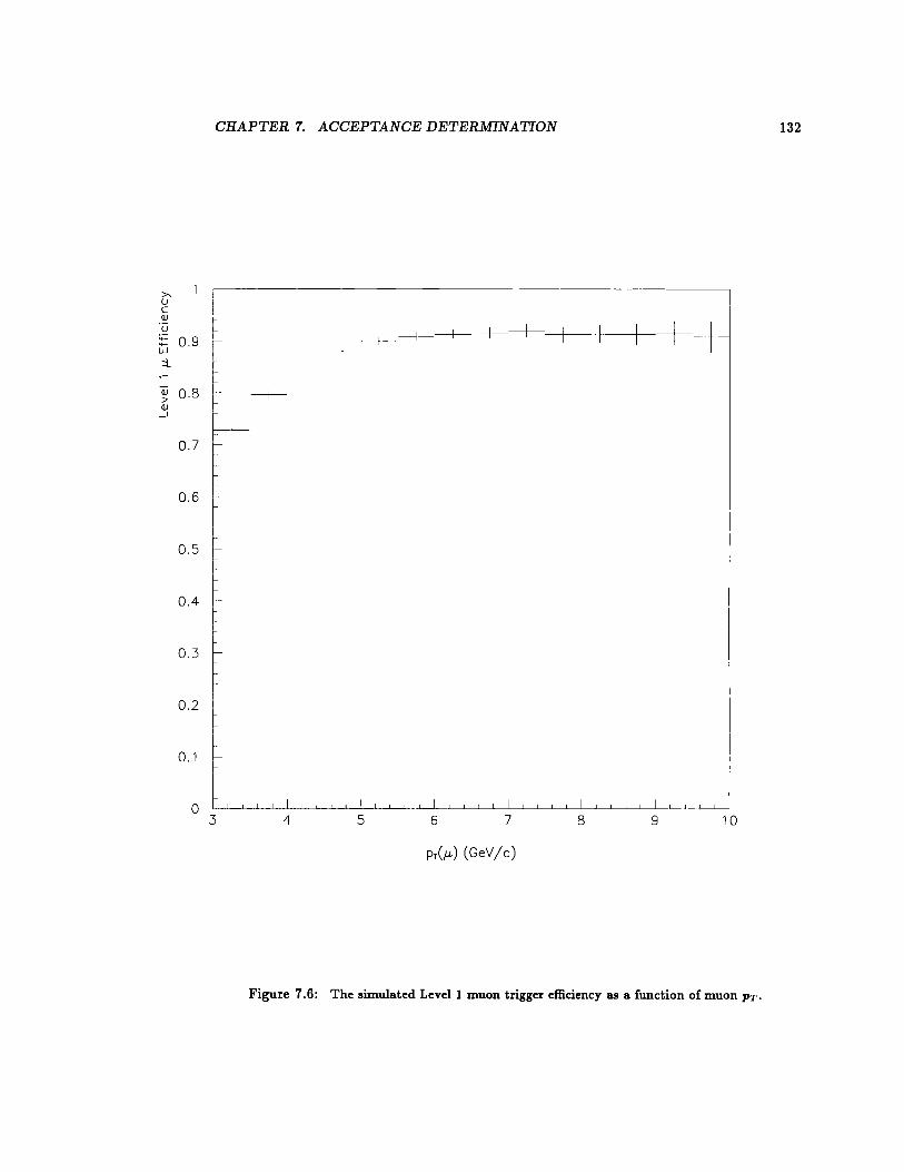
CHAPTER 7. ACCEPTANCE DETERMINATION 132
- -----
>- I u ~ c
Q)
~ I ·u 1--+-4- 0.9 --+---1---+-- -----r--w I ::i_
~ Qj 0.8 --+--> Q) _j
0.7
0.6
0.5 -
0.4 -
0.3
0.2
0.1
0 3 4 5 6 7 8 9 10
Pr(J..L) (GeV/c)
Figure 7.6: The simulated Levell muon trigger efficiency as a function o£ muon PT·
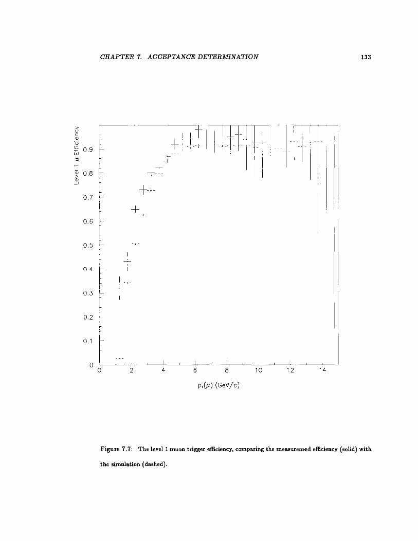
CHAPTER 7. ACCEPTANCE DETERMINATION 133
>
+I~~--~ !_ft1f_1 u c: ~ Q)
"() :;: 0.9
~ w t~-- ~ I :::l_
03 0.8 ~ i > L
T~-~
Q) _j +r-
0.7
+ T ~
0.6 ~-
0.5 [_
I r --1-'
0.4 I
I -,-'
0.3
0.2 ,-
0.1 ~ 0 0 2 4 6 8 10 12 14
Pr(!l-) (GeV/c)
Figure 7.7: The level! muon trigger efficiency, comparing the measuremed efficiency (solid) with
the simulation (dashed).
CHAPTER 7. ACCEPTANCE DETERMINATION 134
- -- ----- -~-~-
"' I u teooo L
i QJ I
2 i '<!-
t~ '-QJ Q_
I :::l_
' 13ooo I I
I I t
6000
4000
2000
2.92 2.96 3 3.04 3.08 3.12 3.16 3.2 3.24 3.28
Figure 7.8: The simulated dimuon mass.
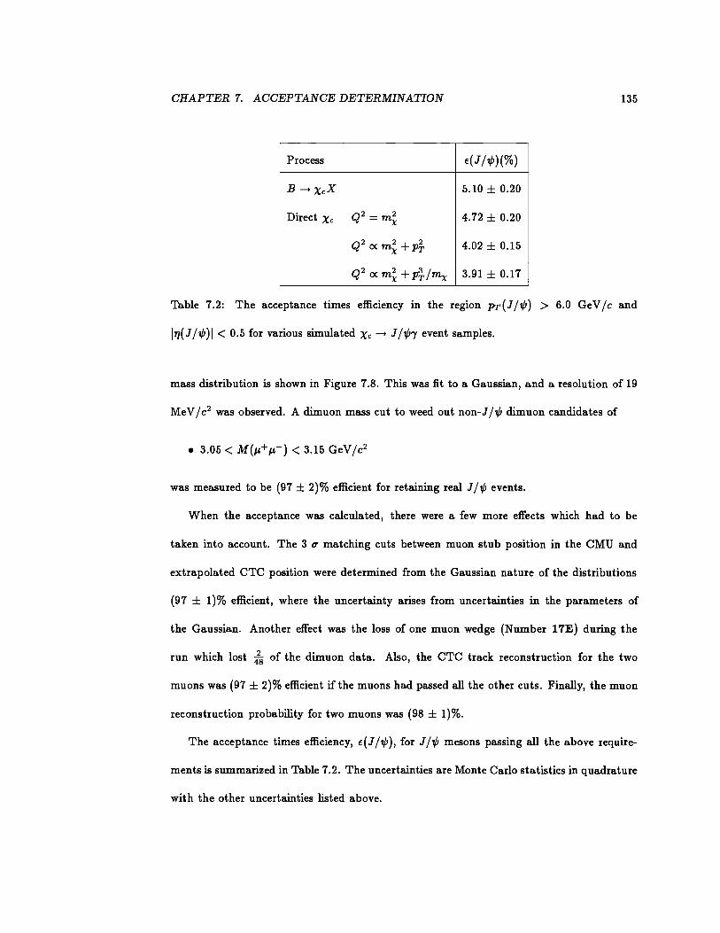
CHAPTER 7. ACCEPTANCE DETERMINATION 135
Process E(J N)(%)
B---+ XcX 5.10 ± 0.20
Direct Xc Q2 =m~ 4.72 ± 0.20
Q2 oc m~ + p} 4.02 ± 0.15
Q2 oc m~ + p~fmx 3.91 ± 0.17
Table 7.2: The acceptance times efficiency in the region PT(Jj,P) > 6.0 GeV/c and
177(1/t/J)I < 0.5 for various simulated Xc---+ 1/t/J'Y event samples.
mass distribution is shown in Figure 7.8. This was fit to a Gaussian, and a resolution of 19
MeV jc2 was observed. A dimuon mass cut to weed out non-J /1/J dimuon candidates of
• 3.05 < M(p.+p.-) < 3.15 GeV jc2
was measured to be (97 ± 2)% efficient for retaining real J /1/J events.
When the acceptance was calculated, there were a few more effects which had to be
taken into account. The 3 u matching cuts between muon stub position in the CMU and
extrapolated CTC position were determined from the Gaussian nature of the distributions
(97 ± 1)% efficient, where the uncertainty arises from uncertainties in the parameters of
the Gaussian. Another effect was the loss of one muon wedge (Number 17E) during the
run which lost 428 of the dimuon data. Also, the CTC track reconstruction for the two
muons was (97 ± 2)% efficient if the muons had passed all the other cuts. Finally, the muon
reconstruction probability for two muons was (98 ± 1)%.
The acceptance times efficiency, E(J /1/l), for J /1/J mesons passing all the above require-
ments is summarized in Table 7.2. The uncertainties are Monte Carlo statistics in quadrature
with the other uncertainties listed above.
CHAPTER 7. ACCEPTANCE DETERMINATION 136
7.2.4 Photon Geometry Simulation
The photon geometry cuts were simulated as well. The photon geometry simulation began
with the same generated event vertex as the muon geometry simulation. From this and the
photon momentum given by the Monte Carlo generator, the photon shower position in the
CES was calculated. The fiducial requirements were the same as for the Xc reconstruction:
• The photon hit at least 9 em in z from the joining oft he two 1J halves of the calorimeter
at 90° from the beamline
• The photon hit within 21 em from the center of a CEM tower in the r - ¢ direction
to avoid the cracks between wedges
• The photon hit in the most central region of the CEM, 55° < detector 8 < 125°
• The photon did not fall into the same calorimeter tower as either muon
7.2.5 Photon Efficiency Simulation
The photon energy spectrum for events passing all J /1/J and photon geometry requirements
was different for each Monte Carlo sample. Because the photon efficiency is also energy
dependent, the difference in photon energy spectra of these samples implies that the in-
tegrated average photon efficiency will be different for each sample. It should be noted
that the J /1/J selection requirements, which preferentially select higher PT J /1/J mesons, and
therefore higher PT Xc mesons, will bias the average photon energy to a higher value than for
events without the J /1/J cuts. This is why the total efficiency is determined for each process
separately, taking into account the correlations between all the generated decay products.
The photon efficiency was simulated using the efficiency curve for the photon (shown
in Figure 6.21). Each event was weighted by the value of the efficiency for the energy bin
CHAPTER 7. ACCEPTANCE DETERMINATION 137
the photon fell into. The weight was zero if the photon failed the geometry requirements
listed above. The weights were summed for events passing all the J /'1/J requirements, and
the average efficiency was just this sum divided by the number of events. Thus, the photon
acceptance times efficiency, e( r), was determined by the equation
"!'f(Jf.p) w(E ) ( )
~.-1 7 f "Y = N(JN) (7.4)
where w( E7 ) is the efficiency weight which depends upon the energy and position of the
photon and N(J/,P) is the number of events passing all the Jj,P requirements. The product
of e(r) and e(J /'1/J) was the total Xc acceptance times efficiency e. This was a simple product
since the J /,P requirements were made first (both in the Monte Carlo and the data) and
then the photon requirements were made after the J / ,P had already been reconstructed. The
values for e(r) and e for the different Monte Carlo runs are summarized in Table 7.3, along
with the relative fractions of each Xc state reconstructed. The importance of determining
different values of e for the various assumptions for Q2 was primarily to show that the
central value obtained for direct production ( e calculated with Q2 oc mi + p}) was not close
to a non-linear dropoff of efficiency that a slightly different 'PT spectrum would experience.
The relatively linear progression off with the exponent on 'PT shows that such a non-linear
dropoff does not exist near the kinematic region generated. An estimate of the magnitude
of the uncertainty in f arising from uncertainties in the underlying Xc 'PT distribution will
be found in Section 7.3.
7 .2.6 Xc Polarization
The unknown polarization of the Xc mesons introduced another uncertainty in the accep-
tance calculation. If the angle of the r momentum direction, boosted into the Xc rest frame
with respect to the Xc momentum direction was()*, the similar angle for the J /'1/J was -9*.
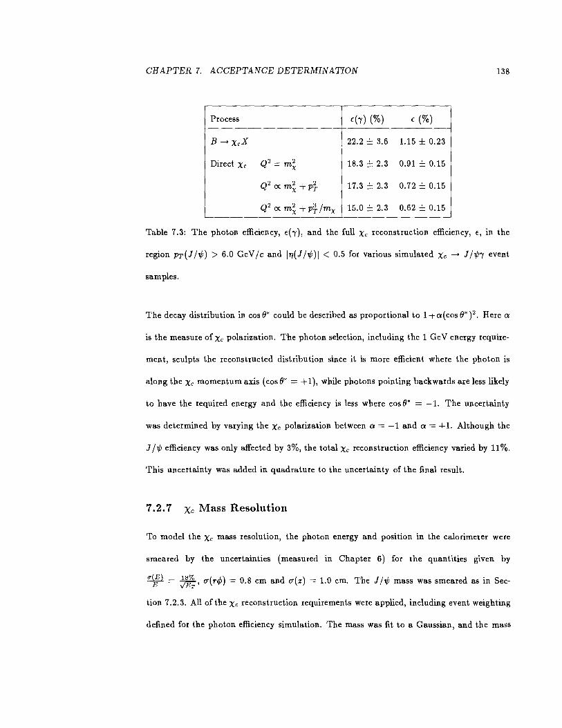
CHAPTER 7. ACCEPTANCE DETERMINATION 138
Process E(l) (%) E (%)
B----+ XcX 22.2 ± 3.6 1.15 ± 0.23
Direct Xc Q2 _ m2 - X 18.3 ± 2.3 0.91 ± 0.15
Q 2 ex m~ + p} 17.3±2.3 0.72 ± 0.15
Q 2 ex m~ + p'f/mx 15.0 ± 2.3 0.62 ± 0.15
Table 7.3: The photon efficiency, E('i'), and the full Xc reconstruction efficiency, E, in the
region PT(l N) > 6.0 GeV /c and I11(J N)l < 0.5 for various simulated Xc ----+ J N1 event
samples.
The decay distribution in cosO• could be described as proportional to 1+a(cos6*)2 • Here a
is the measure of Xc polarization. The photon selection, including the 1 Ge V energy require-
ment, sculpts the reconstructed distribution since it is more efficient where the photon is
along the Xc momentum axis (cos 6* = + 1 ), while photons pointing backwards are less likely
to have the required energy and the efficiency is less where cos 6* = -1. The uncertainty
was determined by varying the Xc polarization between a = -1 and a = + 1. Although the
J /..P efficiency was only affected by 3%, the total Xc reconstruction efficiency varied by 11%.
This uncertainty was added in quadrature to the uncertainty of the final result.
7.2.7 Xc Mass Resolution
To model the Xc mass resolution, the photon energy and position in the calorimeter were
smeared by the uncertainties (measured in Chapter 6) for the quantities given by
uVf) = J-2-, u(r¢) = 0.8 em and u(z) = 1.0 em. The J /..P mass was smeared as in Sec-
tion 7.2.3. All of the Xc reconstruction requirements were applied, including event weighting
defined for the photon efficiency simulation. The mass was fit to a Gaussian, and the mass
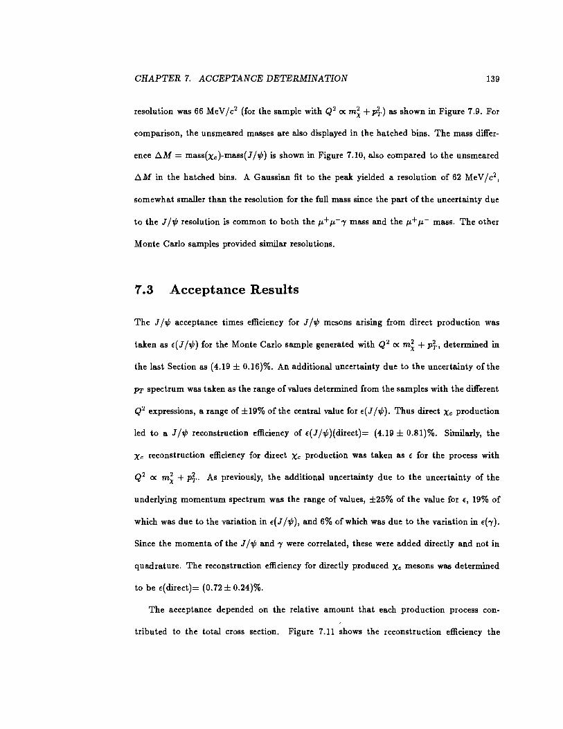
CHAPTER 7. ACCEPTANCE DETERMINATION 139
resolution was 66 MeV /c2 (for the sample with Q2 ex m~ + p}) as shown in Figure 7.9. For
comparison, the unsmeared masses are also displayed in the hatched bins. The mass differ-
ence ll.M = mass(xc)-mass(J/,P) is shown in Figure 7.10, also compared to the unsmeared
ll.M in the hatched bins. A Gaussian fit to the peak yielded a resolution of 62 MeV fc2 ,
somewhat smaller than the resolution for the full mass since the part of the uncertainty due
to the J/,P resolution is common to both the JL+JL-'Y mass and the JL+JL- mass. The other
Monte Carlo samples provided similar resolutions.
7.3 Acceptance Results
The J /,P acceptance times efficiency for J /,P mesons arising from direct production was
taken as E(J /,P) for the Monte Carlo sample generated with Q2 ex m~ + p}, determined in
the last Section as (4.19 ± 0.16)%. An additional uncertainty due to the uncertainty of the
PT spectrum was taken as the range of values determined from the samples with the different
Q2 expressions, a range of ±19% of the central value for E(J /,P). Thus direct Xc production
led to a J N reconstruction efficiency of E(J /tP)(direct)= (4.19 ± 0.81)%. Similarly, the
Xc reconstruction efficiency for direct Xc production was taken as € for the process with
Q2 ex m~ + p}. As previously, the additional uncertainty due to the uncertainty of the
underlying momentum spectrum was the range of values, ±25% of the value for E, 19% of
which was due to the variation in E(J N), and 6% of which was due to the variation in E('Y).
Since the momenta of the J / ,P and 'Y were correlated, these were added directly and not in
quadrature. The reconstruction efficiency for directly produced Xc mesons was determined
to be €(direct)= (0.72 ± 0.24)%.
The acceptance depended on the relative amount that each production process con-
tributed to the total cross section. Figure 7.11 shows the reconstruction efficiency the
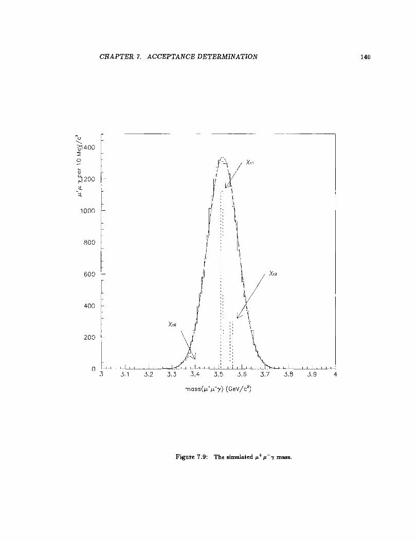
CHAPTER 7. ACCEPTANCE DETERMINATION
"'u r ~400 ~ 0
L. QJ
~200 ~ ':::t +:::l..
1000
800
600 -
400 -
200
0 3 3.1 3.2 3.3 3.4 3.5 3.6 3.7 3.8
Figure 7.9: The simulated 11-+ 11--'Y mass.
140
3.9 4
CHAPTER 7. ACCEPTANCE DETERMINATION
Nu L '-.... > Q)
::2 0 1400 1.... Q) Q_
r ~::i1200 -
::l_
1 000 1--1
800
600 ~ I
400
200
0 0
X co
0.1
\
0.2 0.3
(\1 Xcl
II 1 I !i \
I !! \
I :: \/ x,, ,, '' ,, ,. '' ' ,, ,,
'' '' ,, '' ,,
0.4 0.5 0.6 0.7 0.8
Figure 7.10: The simulated ll.M distribution.
141
-~
0.9
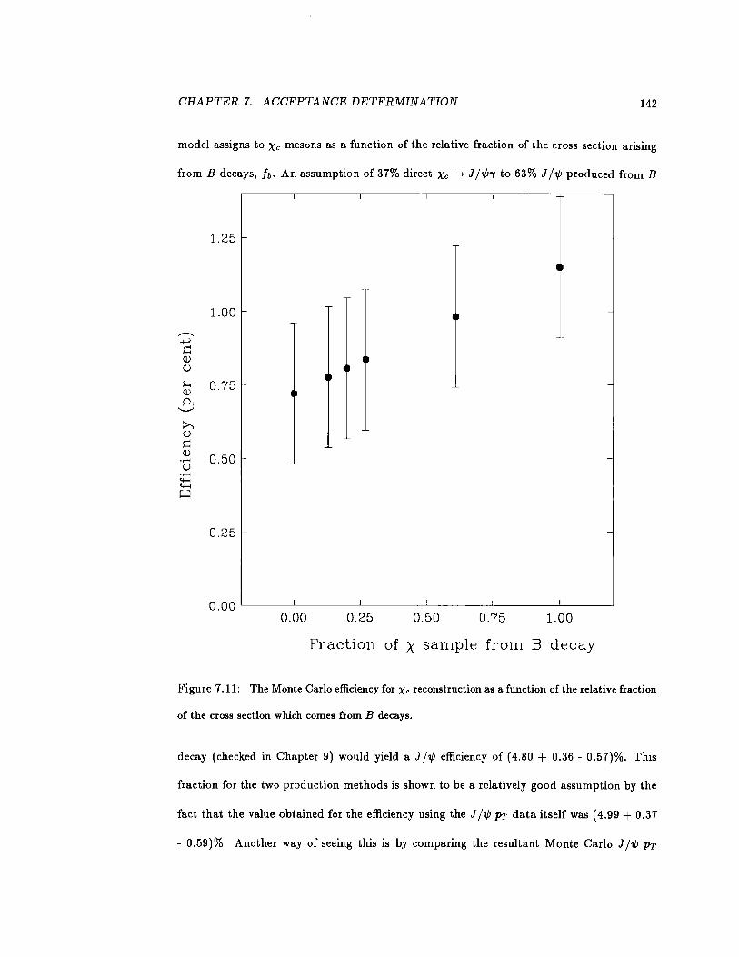
CHAPTER 7. ACCEPTANCE DETERMINATION 142
model assigns to Xc mesons as a function of the relative fraction of the cross section arising
from B decays, fb· An assumption of 37% direct Xc --+ J /1/Jr to 63% J /1/J produced from B
1.25 -
~~
1.00 -
,......-., ...,__, ~ Q) ()
s.... 0.75 -Q) ~~~ 0, ..__., >.. ()
~ Q) 0.50 - -...... () ...... ....... .......
j:£1
0.25
O.OOL_ ____ L_ ______ L_ ______ ~----~L-----~L---~
0.00 0.25 0.50 0.75 1.00
Fraction of x sample from B decay
Figure 7.11: The Monte Carlo efficiency for Xc reconstruction as a function of the relative fraction
of the cross section which comes from B decays.
decay (checked in Chapter 9) would yield a J N efficiency of ( 4.80 + 0.36 - 0.57)%. This
fraction for the two production methods is shown to be a relatively good assumption by the
fact that the value obtained for the efficiency using the J /1/J PT data itself was (4.99 + 0.37
- 0.59)%. Another way of seeing this is by comparing the resultant Monte Carlo J /1/J PT
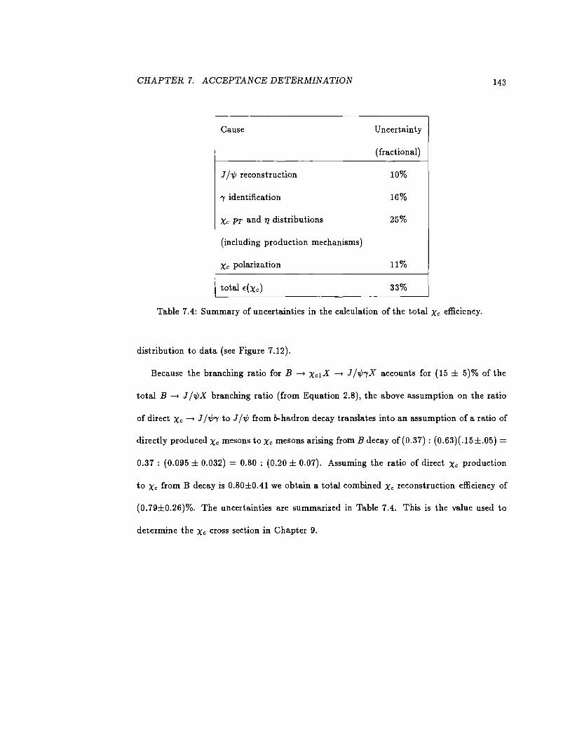
CHAPTER 7. ACCEPTANCE DETERMINATION 143
Cause Uncertainty
(fractional)
J /1/J reconstruction 10%
'Y identification 16%
Xc PT and 1J distributions 25%
(including production mechanisms)
Xc polarization 11%
total E(Xc) 33%
Table 7.4: Summary of uncertainties in the calculation of the total Xc efficiency.
distribution to data (see Figure 7.12).
Because the branching ratio for B --> XclX --> J /1/J'YX accounts for (15 ± 5)% of the
total B --> J j,PX branching ratio (from Equation 2.8), the above assumption on the ratio
of direct Xc --> J /1/J'Y to J /1/J from b-hadron decay translates into an assumption of a ratio of
directly produced Xc mesons to Xc mesons arising from B decay of(0.37): (0.63)(.15±.05) = 0.37 : (0.095 ± 0.032) = 0.80 : (0.20 ± 0.07). Assuming the ratio of direct Xc production
to Xc from B decay is 0.80±0.41 we obtain a total combined Xc reconstruction efficiency of
(0.79±0.26)%. The uncertainties are summarized in Table 7.4. This is the value used to
determine the Xc cross section in Chapter 9.
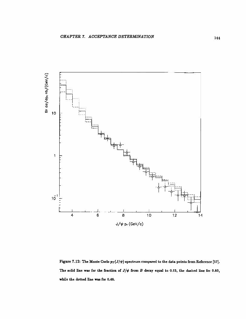
-u ......... :::; (!) -.J ......... .0 r:;
a. "'C ......... b
"'C ... m 10
-1 10
CHAPTER 7. ACCEPTANCE DETERMINATION 144
J/1/1 Pr (GeV/c)
Figure 7.12: The Monte Carlo PT(J/,P) spectrum compared to the data points from Reference [57].
The solid line was for the fraction of J /,P from B decay equal to 0.63 1 the dashed line for 0.801
while the dotted line was for 0.46.
Chapter 8
Reconstruction of the xc
Mesons
8.1 Selection of J /1/J Sample
The event selection for this analysis began with the definition of a J /1/J data sample from
the decay J /1/J --+ 11-+ 1£-. This technique exploited the easily implemented 11-+ 11-- trigger.
The identification of two muons from the decay of quarkonia produced an especially clean
event sample. The J /1/J sample obtained was the starting point of many measurements at
CDF. For instance, B to J /1/J decays have been reconstructed at CDF [11, 12]. Herein is
presented the reconstruction of Xc --+ J /1/J"f.
8.1.1 Definition of JL Candidates
Muon candidates were defined through a procedure which matched tracks in the CTC to
stubs in the muon chambers. Such a matching produced a muon candidate because hadrons
145
CHAPTER 8. RECONSTRUCTION OF THE xc MESONS 146
and electrons were not typically able to penetrate the 5.5 interaction lenghts of material
between these detector elements, whereas a muon could. Also, track quality requirements
on the relative positions and angles of the CTC track and muon chamber stub helped to
further isolate the real muons from hadron punchthrough, particle decays and other fake
events.
The uncertainty in the track matching after passage through the calorimeters was dom-
inated by multiple Coulomb scattering for muons with momentum less than 20 GeV I c and
by chamber resolution for muons of higher momenta. In a given amount of material of thick-
ness, L, the angle of incident charged particles would be changed by multiple scattering to
a Gaussian distribution centered on the initial angle. The width of this distribution was
given by [4]
13.6MeVIc ITI-uq, = Z;ncvLILR[1 + 0.038 ln(LILR)].
f3p (8.1)
Here Ll LR was the number of radiation lengths traversed, p was the momentum of the
particle, f3 was the ratio of the velocity of the particle to the velocity of light, vIc = PIE,
and Zinc was the charge of the incident particle, i.e. Zinc =1 for muons.
For the material in CDF this reduced to (58]
13.8cm rr1, = ---vo.59 + 0.41lsin8.
PT
Once energy loss in the calorimeter was taken into account, this became [58]
U'J, = 13.8cm PT
0.59 + 0.41 I sin(} 1- 0.71IPT
(8.2)
(8.3)
Upon including detector resolution effects, the final width of the matching in the x
direction became [58]
2 ( 13.8cm) 2 0.59 + 0.41lsin8 ( )2 u1 = I + 0.3cm . " PT 1-0.71 PT
(8.4)
CHAPTER 8. RECONSTRUCTION OF THE xc MESONS 147
The first term in the above expression was due to multiple scattering. At a momentum
of 4 GeV lc perpendicular to the beam direction its magnitude was about (3.8cm) 2 • The
second term was due to detector resolution effects. The momentum for calculating the
expected spread in matching UJx was calculated from the CTC helix parameters for the
track associated with the CMUO. The width of the difference in slope in the x direction was
expected to be
2 -(0.131) 2 0.27+0.73lsin8 ( )2 u 5 - -- I + 0.0062 . "' PT 1 - 1.43 PI'
(8.5)
The width of the difference in the local CMU z position was calculated to be
2 ( 13.8cm )2 0.59 + 0.411 sin() 1 ( )2 u1 = + 1.5cm . • 'PT 1- 0.71IPT (sin8) 2 (8.6)
Finally, the difference in slope in the z-y plane was calculated to have a width
2 (0.131) 2 0.27+0.73lsin9(. ()) 2 ( ) 2 u 5 = -- I szn + 0.14 . z 'PT 1 - 1.43 'PT
(8.7)
Muons with momenta less than approximately 1.43 GeV lc ranged out in the CDF detector,
that is they stopped before reaching the muon chambers.
These variables were measured for CMUO's by propagating the CTC track to the associ-
a ted CMU wedge. This propagation included the effects of the solenoid magnetic field value
and radius, the geometry of the calorimeter, the expected return field, and the geometry
of the central muon detectors. The difference in the propagated position and the measured
stub position defined the matching variables. The difference in local CMU coordinates in
the x direction was Ix, and Iz in the local z direction. The difference in expected slope in
the x-y plane relative to that of the stub was Sx, and Sz in the z-y plane.
A variable for determining the significance of the matching of the track to the muon
stub was defined. This included alignments of the detector elements and values of the
CHAPTER 8. RECONSTRUCTION OF THE xc MESONS 148
return fields. The significance of the matching in the x-y plane was defined as
(8.8)
The significance for z-y matching was
(8.9)
Studies indicated that fake muon tracks from hadron punchthrough and other sources gen-
erally had a poor matching in several of these variables, so cuts on all of them were not
required. Specifically, for the final muon identification, only the cuts IM1~ I :S: 3.0 and
IM1.I :S: 3.0 were needed. The efficiency of requiring events described by a Gaussian distri-
bution to be within 3 (J' of the mean was taken to be 99.73 %.
A small number of events were discarded due to a hardware problem. Occasionally, an
ADC overflow in the z determination for the CMUO occured which meant the z coordinate
could not be determined. For the sake of event sample purity such tracks were eliminated.
The efficiency including CMUO reconstruction and no ADC overflow was determined to be
96.7 ± 0.7 %.
These cuts gave a muon sample definition. Since J /1/J candidates were the tag for the
signal, events with 2 muon candidates as defined above were examined.
8.1.2 Dimuon Sample
The analysis started by identifying two muon candidate tracks which came from the decay
of a J /,P meson. An algorithm to loop over all muon candidate pairs was used for this
identification. All dimuon combinations with opposite charge were examined for consistency
with the hypothesis that they came from a J / ,P decay.
First, each muon candidate's CTC track was associated with a z vertex in the track
reconstruction. Both muon candidate tracks were required to be associated with the same

CHAPTER 8. RECONSTRUCTION OF THE xc MESONS 149
vertex number so tracks from different interactions would not fake a J /1/J signal. Additional
cuts were motivated by the specifics of the trigger and the understanding of the trigger
efficiency.
Data selection included a trigger requirement. The CDF trigger system has been dis-
cussed in detail in Chapter 4. CDF ran with a complex trigger table involving many triggers,
some of which used information from the central muon chambers. For J /1/J reconstruction,
the dimuon_central_3 trigger was used. All events for this analysis were required to have
passed the dimuon_central_3 trigger.
As previously noted (see Chapter 4), the dimuon_central_3 trigger started with the level
one central_muon__3 trigger, which was a 3 GeV /c single muon trigger. The transverse mo-
mentum was determined using the beam constraint described in Section 5.2. The efficiency
of this trigger plateaus at about 92 ± 3% for PT > 6.0 GeV jc. (Figure 4.2). This motivated
a cut of 3 GeV /c for the transverse momentum of all muon candidates obtained from the
data which passed the dimuon_central_3 trigger. This was the first cut motivated by an
understanding of the trigger.
The level 2 dimuon_central_3 trigger chose "gold muons" (defined in Chapter 4) in the
hardware decision making process. Since any measurements obtained with this trigger relied
on an understanding of the efficiency of the trigger, only events which contributed to the
level 2 trigger were used to form J /1/J candidates. All muon candidates were required to fall
in a wedge tagged as a gold muon wedge.
A wedge geometry cut was motivated by the trigger. As noted previously, the gold muon
wedges were clustered for use in the dimuon_central_3 trigger. This resulted in events with
muons in neighboring wedges not causing the level 2 trigger to latch. The dimuon efficiency
was understood only for dimuons that helped the event pass the trigger. For instance,
in events with 3 or more muons, the number of dimuons contributing to the trigger cross
CHAPTER 8. RECONSTRUCTION OF THE xc MESONS 150
section could have been overestimated unless the gold muon wedge requirement was applied.
Therefore, the muon pairs in consideration were required to not be in adjacent wedges.
The definition of adjacent was the same as for gold muon wedge clustering. Muons were
considered adjacent if they were in the exact same wedge, or although in different wedges
in 1J they were the same in ¢, or if in the same 1J side they were in the next wedge over in
¢. The dimuons that pass these requirements would have caused the trigger to latch.
As seen in Chapter 7, the efficiency for J /..P reconstruction dropped off significantly for
values of pseudorapidity above 1J = 0.5 (Figure 7.4). Because the efficiency should be well
understood for any analyis using J /..P candidate events, all dimuon events were required to
have a dimuon pseudorapidity in the region 1111 :S 0.5.
These cuts gave a sample of dimuon events for which the trigger efficiency was under-
stood. The cuts are summarized here: 1) The position matching of the muon stubs with
the associated CTC tracks was required to be measured and :S 3.00" in both (x, y) and (z, y)
views. 2) The 2 muon candidates must have opposite charge. 3) The tracks of the 2 p,
candidates must be associated with the same z vertex. 4) The event must have passed the
dimuon_central_3 trigger. 5) The transverse momentum of each p, must be 2 3.0 GeV fc. 6)
Each p, CMU stub must have fallen in a wedge tagged as a gold muon wedge. 7) The p,+ and
p,- must have fallen into wedges which were not adjacent. 8) The dimuon pseudorapidity
must have fallen in the region 1111 :S 0.5. The dimuon sample thus defined formed the basis
of the data selection for the analysis described here. All pairs of tracks passing these cuts
were thus identified as p,+ p,- events with high purity.
The resolution ofthe central tracking chamber was discussed in Section 5.2. The resulting
error in the determination of transverse momentum was O"pr = J(O.OOllPT )2 + (0.0066F.
The error on cot(O) was O"cot(9) ::::: 0.003. These track resolution effects dominated the
resolution of a particle's momentum vector, p. The momentum vector of each track, Pi,
CHAPTER 8. RECONSTRUCTION OF THE xc MESONS 151
could be found, and an energy could be calculated based on the assumption of the particle
type and mass, Ei = VPi ·Pi+ m?- A four-vector for any pair of tracks could then be
defined, p =~Pi, E = ~Ei, and a pair mass could be calculated, M = ..jE2 - p · p.
The dimuon mass was formed for all events passing the cuts described. Figure 8.1 shows
the mass distribution in the region 2.9::::; M::::; 3.3 GeV/c2 • The 1/1/J resonance is clearly
seen. Also shown is a fit of a Gaussian on a constant background. Figure 8.2 shows the mass
distribution in the region 3.5::::; M::::; 3.9 GeV/c2 (without the above trigger requirements
for more staticstics). The 1/J(2S) resonance is evident. Also shown is the fit of a Gaussian
of the same width and a linear background. The widths of the Gaussians were the same
because the detector resolution was much wider than the natural width of the J /1/J and
1/J(2S). The resolution determined from the Gaussian fit was 18 MeV/c2 • Figure 8.3 shows
the mass distribution in the region 9.0 ::::; M::::; 10.8 GeV /c2 (with some additional isolation
requirements (59]). The individual 1 states (the bb 3 S1 states in Figure 1.5 which can decay
into p,+ p,-) are clearly resolved in this Figure. Also shown is the fit of 3 Gaussians of the
same width and a linear background. The fit allowed the number under each peak, the mass
of each peak, and a common resolution width to vary. The resolution on the 1 states was
50 MeV/ c2 • The masses found from the reconstruction of these resonances was a test on
the mass scale of CDF, because they could be compared to the known values from other
experiments. The fits to the J 11/J, 1/J(2S), 1(1S), 1(2S) and 1(3S) returned mass values of
3.097±0.001, 3.687±0.007, 9.458±0.004, 10.02±0.01 and 10.36±0.01 GeV /c2 respectively,
in agreement with world average values for these particle masses [4) within uncertainties.
8.1.3 The J /'1/J Signal Region
A J /1/J signal region was defined to identify the J /1/J events for further use in this experiment.
The measured J /1/J mass was centered on 3.097±0.001 GeV /c2 , less than one u from the
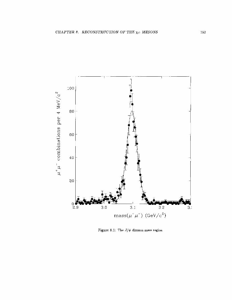
CHAPTER 8. RECONSTRUCTION OF THE Xc MESONS 152
r- ,-T
100 C\l
u ~ > (!)
~
"<:!< 80 ~ (!)
0.. lfJ c 0 60 .......
...,_; ~ c ......
...0 s 0 40 u
I :::t
+ :::t 20
Figure 8.1: The 1/'1/J dimuon mass region
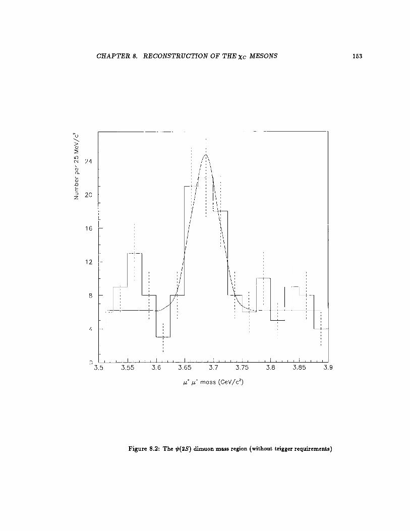
CHAPTER B. RECONSTRUCTION OF THE Xc MESONS
16
8
4
G 3.5 3.6
(\ i ' \ , . I I : ,
~ ~rn~ ~ I, . ,_J ' I ' , I . \ . : , : I\ : :! : 1',1: -1 , U' I \; I \ I :\
3.65 3.7
J_
3.75 3.8 3.85 3.9
Figure 8.2: The ,P(2S) dimuon mass region (without trigger requirements)
153
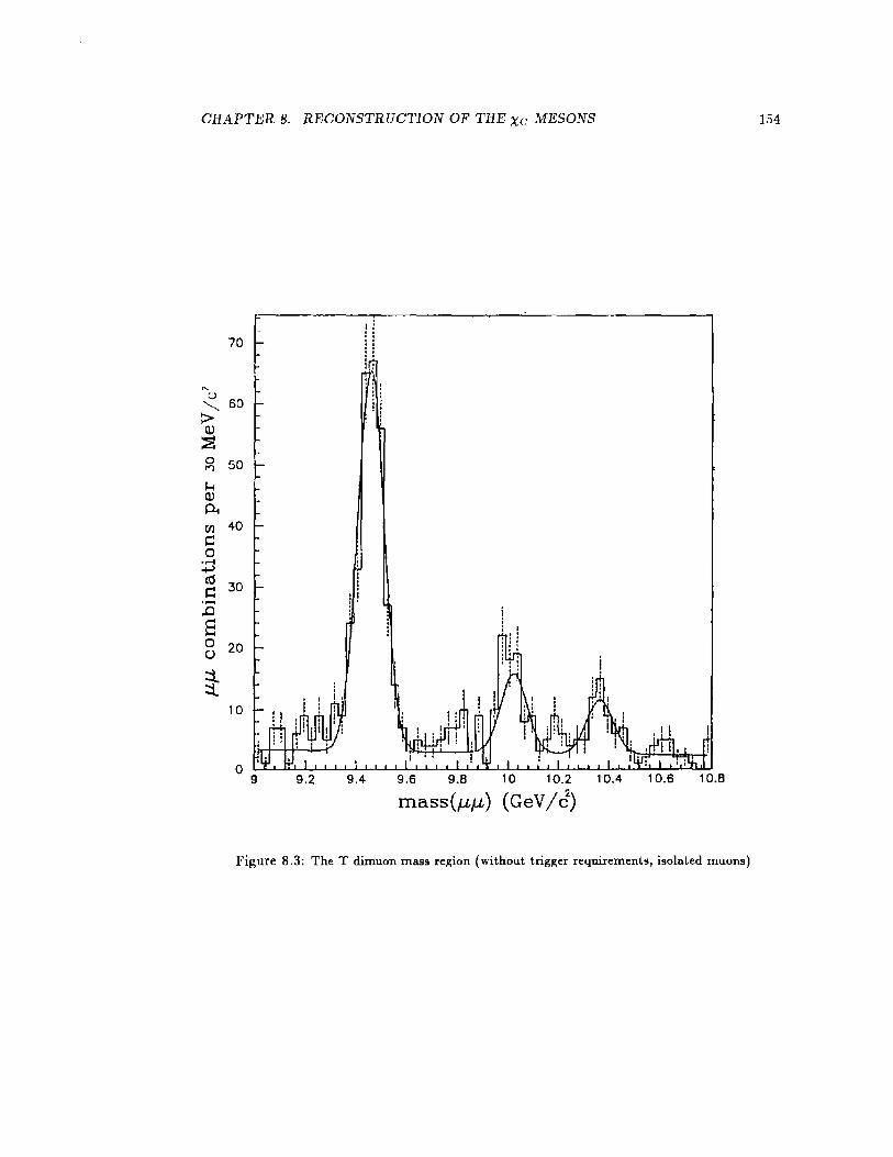
CHAPTER 8. RECONSTRUCTION OF THE xc MESONS 154
70
" u 60 ~ :>
(1)
~ 0 50 I")
~ (1) At rt.l 40 Q 0 ...... ....., td 30 Q ...... .0 s 0 20 C)
~ 10
0 9 9.2 9.4 9.6 9.8 10 10.2 10.4
mass (p.p.) ( Ge V /d)
Figure 8.3: The T dimuon mass region (without trigger requirements, isolated muons)
CHAPTER B. RECONSTRUCTION OF THE xc MESONS 155
world average, and had a resolution width of 18 MeV jc2 • A mass window for the J /1/J
signal was defined from 3.05 to 3.15 GeV/c2 • This mass region is shown as the hatched
area in Figure 8.4. For control, a background sample was obtained of dimuon candidates
which were like those which could have faked the J /1/J signal. This sample came from the
mass sideband regions defined as 2.90 ::; M ::; 3.00 and 3.20 ::; M ::; 3.30. The number of
non-J /1/J events from the sideband regions was 90 ± 16 in a total window of 0.2 GeV jc2 •
Multiplying this by the ratio of the J /1/J signal window width to sideband window width
gives an expected background in the J /1/J window of 45 ± 8. Since there were 941 ± 31
events in the J /1/J candidate region, the number of true J /1/J mesons in the candidate sample
was determined to be 896 ± 32. Another way to determine the number of J /1/J events was
to fit the distribution to a Gaussian with a linear background. The result ofthis fit is shown
in Figure 8.1. The Gaussian contribution corresponds to 907 ± 32 J /1/J events. These two
results agree fairly well with one another.
Many measurements were made starting from this dimuon sample. These J /1/J candidates
were used for the determination of the differential cross section of J /1/J events at Tevatron
energies [57]. Also, they were used to reconstruct many decays, such as ,P(2S) --+ J j,P1r+1r-.
In addition, the decays of heavy quark mesons were reconstructed, such as the decay B;t- --+
J NK+- [11], and B~ --+ J NK 0 * [12]. Presented in this thesis is the reconstruction of
Xc--+ J Nr.
8.2 Reconstruction of the Decay Xc ~ J /'l/Jr
Full reconstruction of the Xc states required not only a J /1/J candidate, but a r candidate
as well. The central electromagnetic calorimeter, consisting of the CEM and CES was used
to identify photons. These photon candidates were used in the Xc analysis.
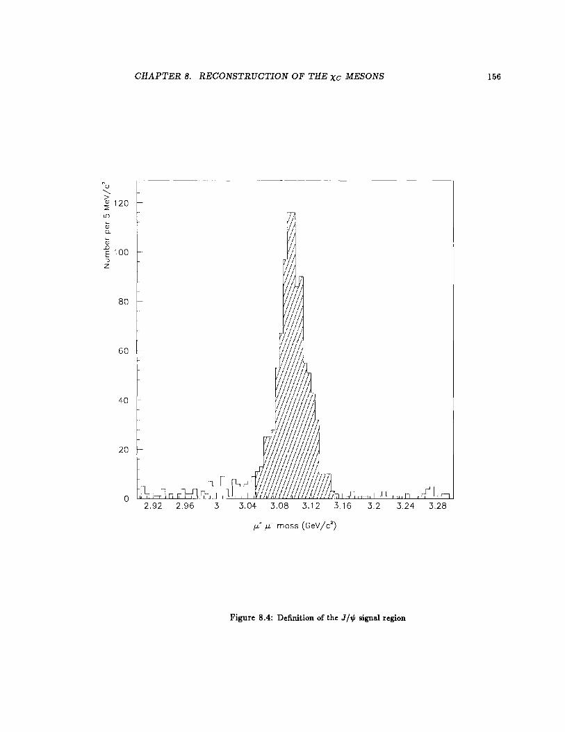
CHAPTER 8. RECONSTRUCTION OF THE xc MESONS 156
N u
~ '---> ~ 120 L[) f
~ '- ·-<J) 0. '-<J)
-E '1oo ::J ~ z
80
60
40
20
0 ,IL,
2.92 2.96 3 3.04 3.08 3.12 3.16 3.2 3.24 3.28
J.L+ J.L- mass (GeV/c')
Figure 8.4: Definition of the J N signal region

CHAPTER 8. RECONSTRUCTION OF THE xc MESONS 157
8.2 .1 Photon Identification
A photon deposited energy in the form of a shower in the electromagentic calorimeter. The
identification of such low energy 1 events required here began with the energy in the CEM.
"Low energy" was defined as well below the calibration energies of 10 to 50 GeV. After
this, the position was found using the strip chamber (CES). The position, in combination
with the determination of the primary vertex, also gave the 1 candidate's direction. The
direction and energy determined the momentum of the I·
Photon identification began by finding electromagnetic energy. All central towers were
examined for energy deposition. Since muons also deposited energy, towers which the muons
traversed were excluded as possible 1 candidate towers. The 1 analysis was continued for
towers with uncorrected energy greater than 0.7 GeV. This cut was the first criterion for
isolation of a 1 candidate sample. The value of 0. 7 Ge V was chosen because the efficiency
for energies below this value dropped sharply. This was discussed in detail in Chapter 6.
Once a tower with at least the minimum energy was identified, a CES cluster match with
the tower was performed. This cluster gave the position information for the 1 candidate. The
strip chamber measured the profile of the electromagnetic shower and the energy deposition
at 6 radiation lengths into the calorimeter.
Associating a CES cluster to the calorimeter tower began by looping over the CES
clusters, produced as noted in Section 5.5. The information calculated for such clusters
included the cluster energy and the position of the cluster in the appropriate 7J or ¢ view.
A CES cluster was required to be in the central region. The cluster was required to be in
the same end of the calorimeter as the tower selected. Due to the geometry of the CES, the
clusters were required to be in the same() half module as the 1 candidate tower. The clusters
were also required to come from the same phi wedge as the tower. The fitted energy of the
CHAPTER B. RECONSTRUCTION OF THE xc MESONS 158
cluster for both the (J and ¢ view was required to be greater than 0. The CES clustering
algorithm gave a fit position of the center of the shower. The closest cluster to the center
of the tower for that view was considered to be the cluster arising from any activity in the
tower. After the loop over the clusters, each view had associated with it a cluster that was
closest to the center of the tower.
The photon candidate direction was defined as the direction vector from the beam posi-
tion at the z vertex of the muons to the position of the CES cluster. The momentum vector
of the photon was defined to have the magnitude of the corrected CEM energy and the di-
rection of the direction vector defined above. The photon energy was taken as the corrected
CEM energy. The momentum and energy thus defined were used as the momentum and
energy of the photon candidate.
There were a few additional cuts on the 1 candidates. First, the photon candidate
energy was required to be greater than 1 GeV. This was motivated by the efficiency of
the photon finding algorithm and the energy resolution (see Chapter 6). Second, for good
measurement of energy, fiducial cuts were performed on the CES clusters. These cuts were
used to exclude regions of the detector which would result in poor measurements, such as
the edge of calorimeters, precisely as performed in Chapter 6. The clusters were required
to be away from the wedge boundaries in ¢, which corresponded to a requirement that the
CES cluster position be within 21 em of the center of the tower in r - ¢. In addition, the
cluster was not used if it was too close to the boundary between the 2 ends, i.e. the crack
at 90 degrees. This boundary was avoided by requiring that the cluster position in z be
greater than 9 em away from the z = 0 plane. Finally, only the first 6 towers on either side
of z = 0 were used. This cut was motivated by an examination of the detector resolution at
these extremely low energies (compared to the energies the CDF calorimeters were designed
for), the expected photon distribution from Xc -> J /..PI decays, and the occupancy of the
CHAPTER 8. RECONSTRUCTION OF THE xc MESONS 159
detectors as the forward region was approached. As mentioned previously, the towers which
the muons traversed were not used. A photon candidate sample with a well measured energy
and momentum was thus ready to be combined with the J /1/J in each event. The energy
distribution of these 1 candidates is shown in Figure 8.5.
8.2.2 Formation of Xc Candidates
The Xc reconstruction then proceeded with the normal combination of 4-vectors. The Xc
candidate momentum vector was just the vector sum of the J /1/J candidate momentum and
the 1 candidate momentum. The energy of the Xc candidate was taken as the sum of the
J /1/J candidate and 1 candidate energies. A mass for the system was then defined as
(8.10)
There was a possibility of some common systematics in the mass combinations of the Xc
and the J /1/J candidates from any mismeasurements in the muon momenta. To minimize
these systematics, a mass difference was used to define the Xc signal region, defined as
D..M = mass(l£+1£-1)- mass(l£+1£-).
Figure 8.6 shows the resulting mass difference spectrum. The full range is visible for the
D..M distribution. There is an excess in the 0 to 1 GeV /c2 bin which will be shown in the
next figure to be explained by the presence of Xc mesons. There is a smoother background
distribution from electromagnetic activity in J /1/J events which rises slowly and then falls
off above 4 to 5 Ge V / c2 . Figure 8. 7 shows the low mass region where the Xc signal would
appear. The peak due to Xc-+ 1/1/JI decays is clearly visible near D..M::::: 0.41 GeVjc2 •
Also shown is the D..M spectrum for the J /1/J sideband region defined above, which was
normalized to the relative mass(l£+ 1£-) window used. No peaking at D..M::::: 0.41 GeV jc2 is
seen in the sideband distribution. The D..M distribution was then used for the final definition
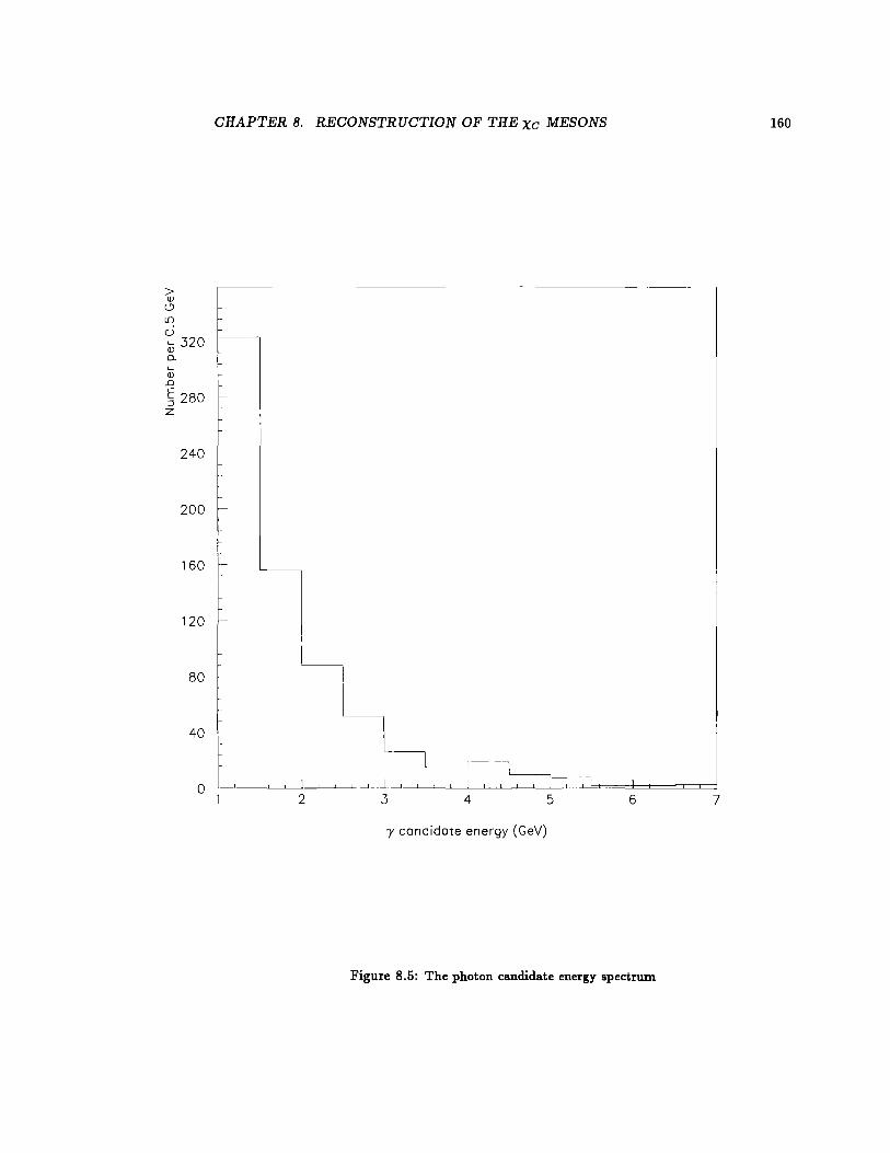
CHAPTER B. RECONSTRUCTION OF THE Xc MESONS
> Q)
C)
L()
0 '- 320 Q) Q_
'-Q) .0
E 280 :J z
240 -
200 -
160
120 -
80
40 -
0
~ L ~ _,--1___
2 3 4 5
-y candidate energy (GeV)
6
Figure 8.5: The photon candidate energy spectrum
160
7
CHAPTER 8. RECONSTRUCTION OF THE xc MESONS 161
of Xc candidates.
8.2.3 Backgrounds
An examination of possible backgrounds in the AM spectrum was necessary to determine
the number ofreconstructed Xc events. Since the contribution from the J /1/J sideband region
was small, it was concluded that most of the background resulted from real J /,P particles
combined with other particles in the event.
The process J N1r0 --+ J NnX
The primary hypothesis as to the source of the background was that it was due to J /1/J7r0 X
where the 1r0 decayed into 'Y'Y and one of these photons combined with the J /1/J. A back-
ground shape was found for this hypothesis by assuming that the kinematics of 1r0 's in
these events would be well modeled by the kinematics of 7r+ and 1r-. Thus, J /,P candidate
events were used with tracks in the same event, assumed to be charged 1r's. A simple Monte
Carlo was then applied for each pion candidate, treating the charged 1r momentum as a 1r0
momentum. A simulated 7r0 --+ 'Y'Y decay at rest was used, and each 'Y was boosted into the
1r reference frame. The energy of the simulated photon as well as the position it would have
in the central electromagnetic calorimetry was calculated.
The AM distribution was reconstructed as if the simulated photon were real. The energy
of the simulated 'Y was required to be greater than 1 Gev. All the J /1/J requirements were the
same as for the Xc reconstruction. A geometric requirement that the photon would have hit
in the same central region used above was applied. In addition, the distribution obtained was
weighted by the photon efficiency (as determined in Chapter 6). The normalization depends
upon the fraction of 1r0 decays which send both photons into the same calorimeter tower
(expected to be about 6% which would lead to an overestimate of the background rate),
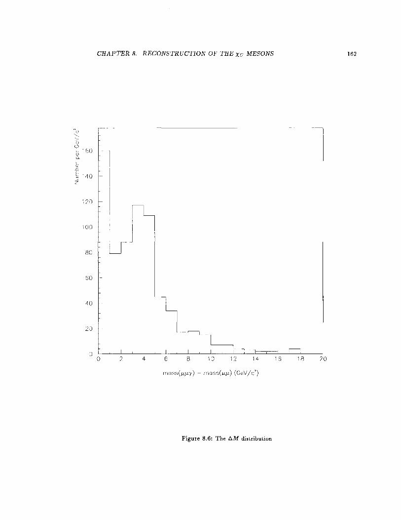
CHAPTER B. RECONSTRUCTION OF THE xc MESONS 162
' <l! _[)
E ·, :10 -~
?
120
100
sc
60
40
20
D 0 2 4 6 8 10 12 14 16 18 70
mass(vJ-Lr) - .TJass(p.,u.) ( GeV / c 2)
Figure 8.6: The l:lM distribution
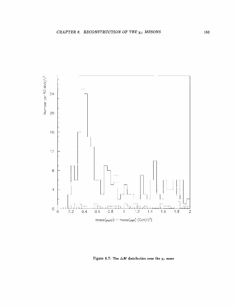
CHAPTER 8. RECONSTRUCTION OF THE xc MESONS 163
N() : "'---- I >
Q)
2 0 Lll 24 L Q) ()_
L Q)
D E ::l 20 z
16
12
8 -
4 l 1-Ul I I
L 0
: ~---I ' ',, 0 0.2 0.4 0.6 0.8 1.2 .4 1.6 1.8 2
moss(JJ-JJ-'Y) - moss(JJ-JJ-) ( GeV / c2)
Figure 8.7: The f:l.M distribution near the Xc mass
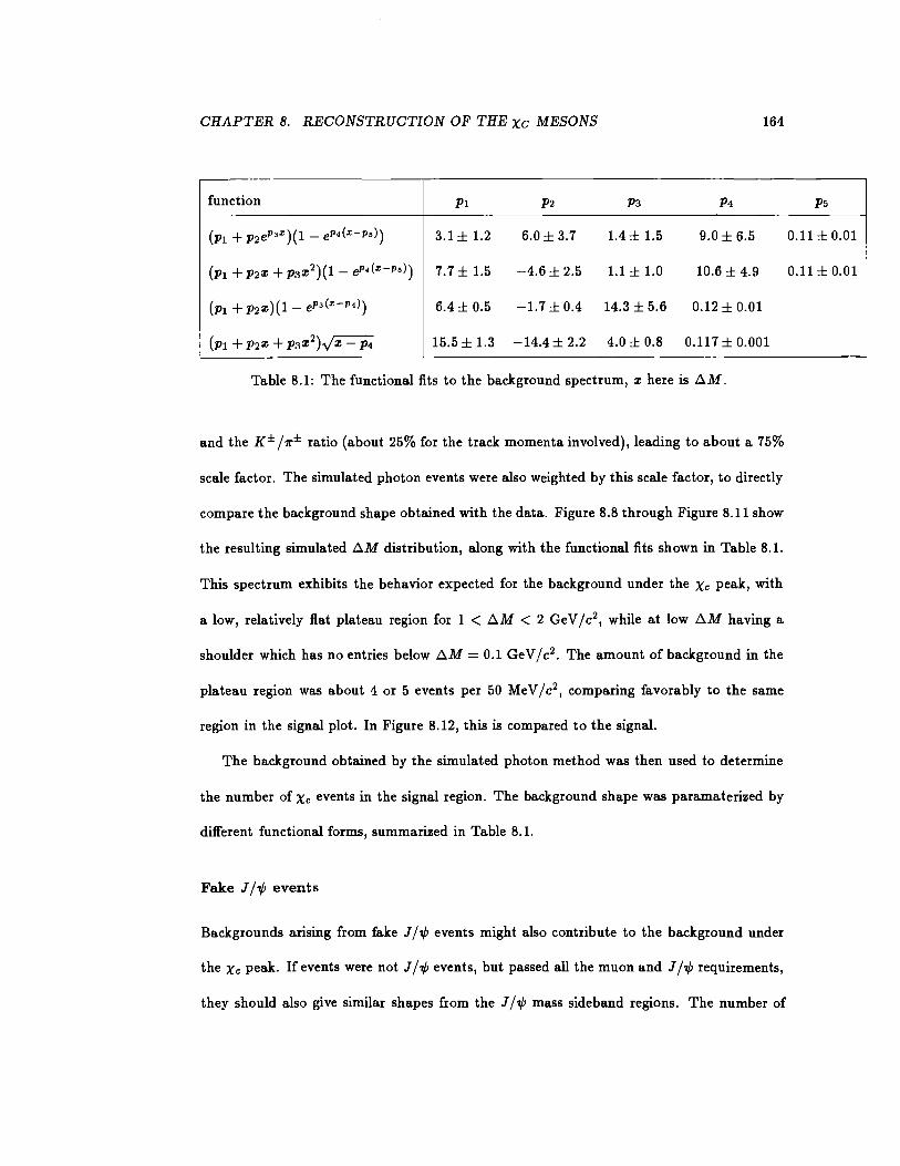
CHAPTER B. RECONSTRUCTION OF THE xc MESONS 164
function P1 P2 P3 P4
(Pl + P2ep'x)(1 - eP•(x-ps)) 3.1 ± 1.2 6.0 ± 3.7 1.4 ± 1.5 9.0 ± 6.5
(Pl + P2Z + P3Z2)(1- eP•(x-ps)) 7.7± 1.5 -4.6 ± 2.5 1.1±1.0 10.6 ± 4.9
(Pi+ P2z)(1- ep,(x-p•)) 6.4 ± 0.5 -1.7±0.4 14.3 ± 5.6 0.12 ± 0.01
(Pl + P2Z + P3Z2)yfz - P4 15.5 ± 1.3 -14.4± 2.2 4.0 ± 0.8 0.117±0.001
Table 8.1: The functional fits to the background spectrum, z here is D.M.
and the K± j1r± ratio (about 25% for the track momenta involved), leading to about a 75%
scale factor. The simulated photon events were also weighted by this scale factor, to directly
compare the background shape obtained with the data. Figure 8.8 through Figure 8.11 show
the resulting simulated Ll.M distribution, along with the functional fits shown in Table 8.1.
This spectrum exhibits the behavior expected for the background under the Xc peak, with
a low, relatively flat plateau region for 1 < D.M < 2 GeV /c2, while at low D.M having a
shoulder which has no entries below D.M = 0.1 Ge V / c2• The amount of background in the
plateau region was about 4 or 5 events per 50 MeV /c2, comparing favorably to the same
region in the signal plot. In Figure 8.12, this is compared to the signal.
The background obtained by the simulated photon method was then used to determine
the number of Xc events in the signal region. The background shape was paramaterized by
different functional forms, summarized in Table 8.1.
Fake J /1/J events
Backgrounds arising from fake J /1/J events might also contribute to the background under
the Xc peak. If events were not J /1/J events, but passed all the muon and J /1/J requirements,
they should also give similar shapes from the J /1/J mass sideband regions. The number of
P5
0.11 ± 0.01
0.11 ± 0.01
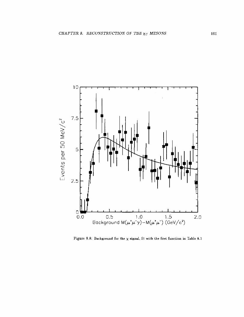
CHAPTER B. RECONSTRUCTION OF THE xc MESONS 165
N 7.5 u ~ > Q)
2 0 lil
5 L Q) 0.. en .......... c Q) > w 2.5
0 .. ~~~~~~~~~~~~~~~~~~~ 0.0 0.5 1.0 1 .5 2.0
Background M(JJ.+JJ.-Y)-M(fJ,+JJ.-) (GeV/c2)
Figure 8.8: Background for the X signal, fit with the first function in Table 8.1
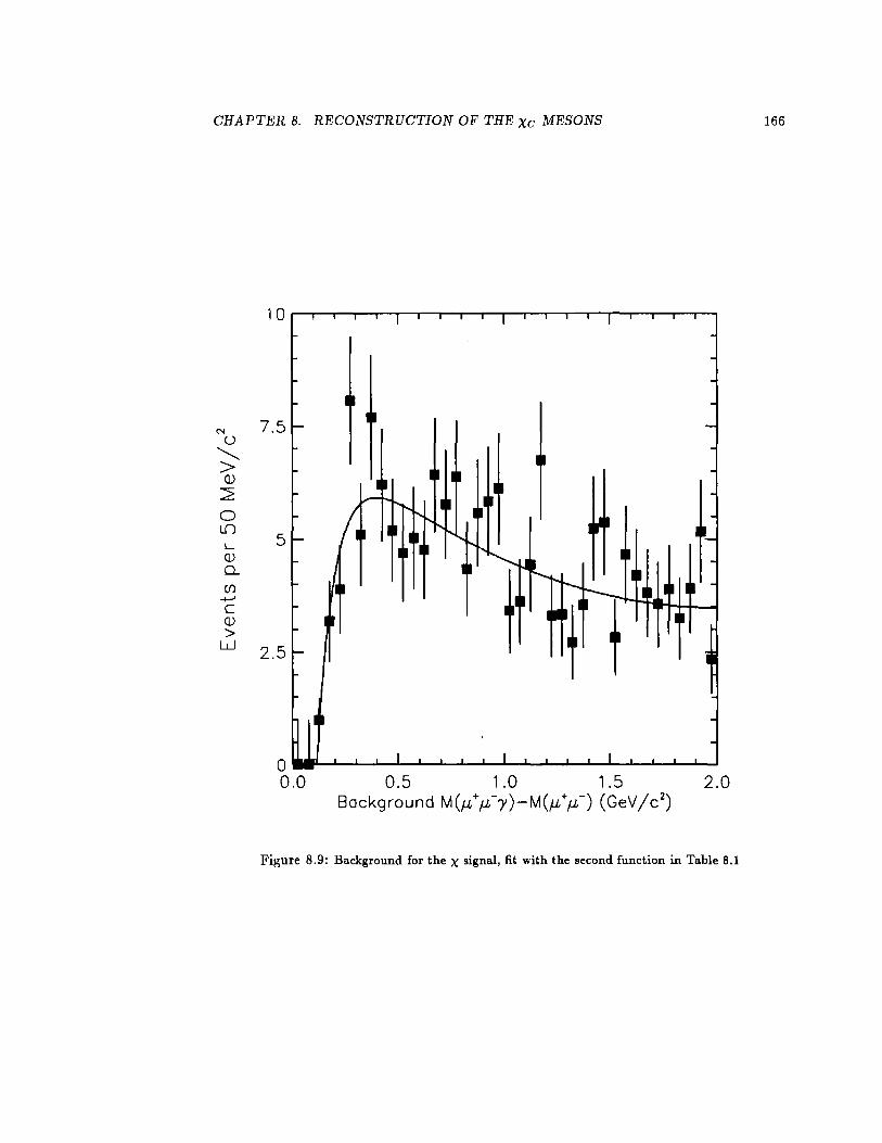
CHAPTER 8. RECONSTRUCTION OF THE Xc MESONS 166
N 7.5 u
"-...._ > Q)
2 0 LO
5 L Q) Q_
(f) +-' c Q) > w 2.5
0 .. ~._~~~~~~~~~~_.~~~--~~~ 0.0 0.5 1 .0 1 .5 2.0
Background M(/.l_+J..L-'Y)-M(/ .. tJ..L-) (GeV / c 2)
Figure 8.9: Background for the x signal, fit with the second function in Table 8.1
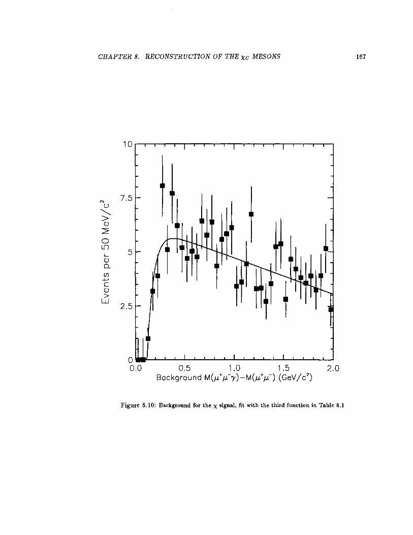
CHAPTER 8. RECONSTRUCTION OF THE xc MESONS 167
N 7.5 u
'-...... > Q)
2 0 L()
5 !..... Q) 0.. CfJ
+-' c Q) > w
2.5
0 .. ~~~~_.~~-L-L~~~~~~~~~ 0.0 0.5 1.0 1.5 2.0
Background M(~J-+/-1--Y)-M(;.i/!J--) (GeV /c2)
Figure 8.10: Background for the x signal, fit with the third function in Table 8.1
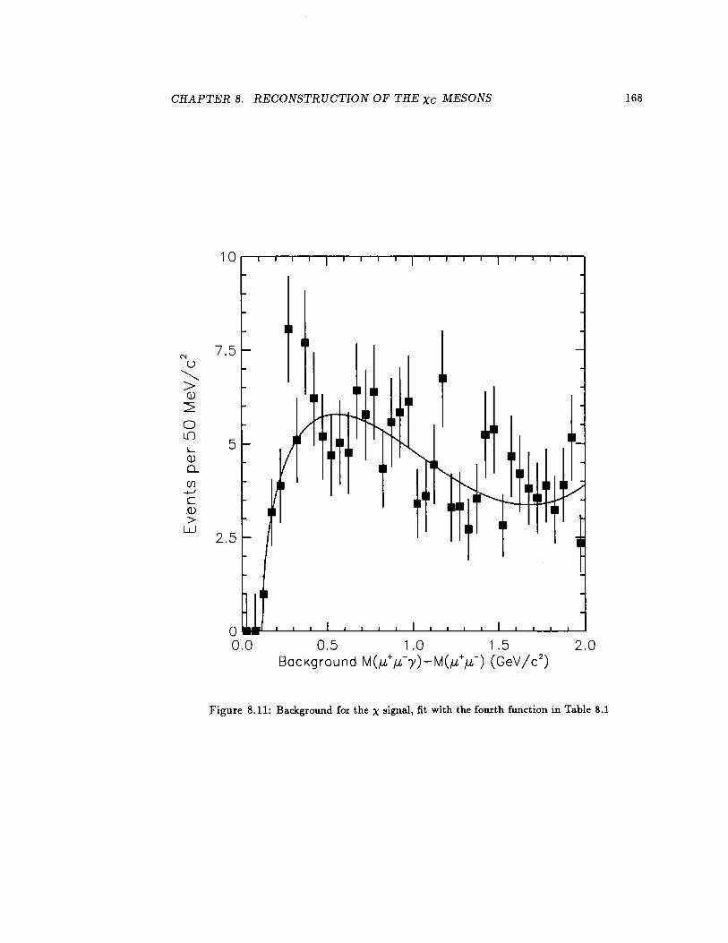
CHAPTER 8. RECONSTRUCTION OF THE xc MESONS 168
"' 7.5
()
~ > Q)
2 0 L[)
5 I,_
Q) 0.. en
-+-' c Q) > w 2.5
0 .. ~~~~~~~~-L~~~~-L-L-L-L~ 0.0 0.5 1.0 1.5 2.0
Background M(J.tJ.L-1')-M(J.L+J.L-) (GeV/c 2)
Figure 8.11: Background for the x signal, fit with the fourth function in Table 8.1
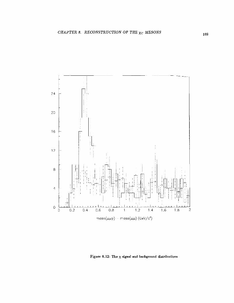
24
20
16
12
8
4
0
CHAPTER 8. RECONSTRUCTION OF THE xc MESONS
0 0.2 0.4
I • I
• I
0.6 0.8
mass(J-<J-<'Y)
1.2 1.4
mass(J-<J-<) ( GeV / c2)
'l:-' ' _L ~
~ : I 1 r i I· I :I I
1.6 1.8
Figure 8.12: The x signal and background distributions
169
2

CHAPTER 8. RECONSTRUCTION OF THE xc MESONS 170
events were shown to be small in Figure 8. 7. This llM distribution from the J /1/J sideband
regions is shown again in Figure 8.13 in a different scale. The events are normalized to the
size of the dimuon mass window. It can easily be seen that the rates for this background is
much smaller than for real J /1/J events including 7i0 decays. Most importantly, however, the
spectrum shows that no peak is produced in the Xc region for this type of background.
Other sources of backgrounds
Other attempts to understand the background proved not as fruitful as the above. If the
J /1/J is combining with activity from a jet, then flipping the J /1/J momentum around a jet
axis would show the same background distribution, while smearing out the llM peak from
real Xc decays. However, the jet axis can only be well understood for jets with energy
greater than 10 GeV or so. The dimuon data sample in the J /1/J region had very few jets
above this energy, so there were not enough statistics to find a background curve. If the
J /1/J momentum is merely flipped 180°, or combined with photon candidates from other
events, the connection with jet activity in the event is lost. Such backgrounds have similar
statistics to the signal, but are much flatter, and showed no peaking effect at small llM.
They were not thought to describe the actual background production reliably. For these
reasons, the 1i0 --+ 'Y'Y background hypothesis was the one used in this analysis to model the
p,+ p,- 'Y candidate background.
8.2.4 The Number of Reconstructed Xc Events
The number of Xc events in the data sample was then determined by fitting the llM spec-
trum to a Gaussian signal over functions describing the background shape. The states
X co, Xc1 ,and Xc2 were not distinguishable due to the resolution. The part of the resolution
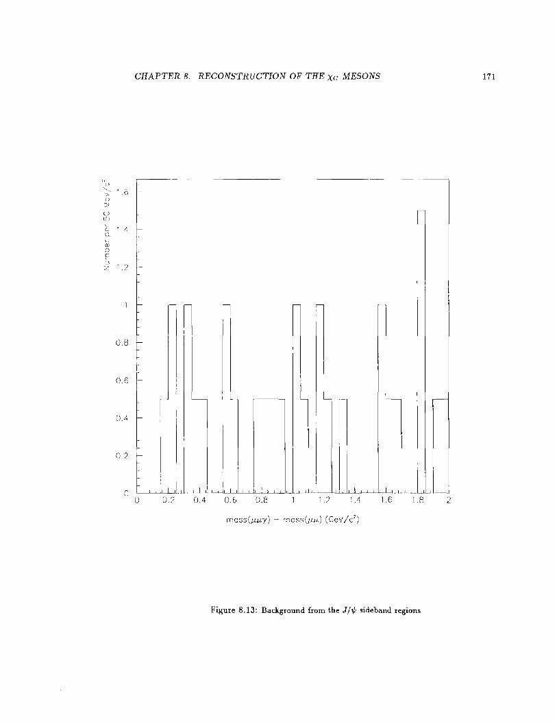
:> [)
(_) L[]
' ~ Q)
_;:]
F
_6
:_' z ~2
0.8
0.6
0.4
()~2
0
CHAPTER 8. RECONSTRUCTION OF THE Xc MESONS
~
n r
-
-
I L__:_..L...c---.L..LI L I D 0.2 0.4
l I
I -
I I
0.6 I
O.B
,--
I
,----I
-
I I I
1./ , 4
mass(JJ-p:y) - r'IOSS(J.L/L) ( GeV / c')
~
I I
~
' ·~
I I 1.6 1.8
Figure 8.13: Background from the J / ,P side band regions
171
I
-
' 2
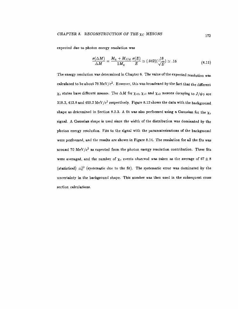
CHAPTER 8. RECONSTRUCTION OF THE Xc MESONS 172
expected due to photon energy resolution was
CT(AM) Mx + M1;.p CT(E) ( )( .18) AM = 2Mx ~ c::: .942 .jE c::: .16 (8.11)
The energy resolution was determined in Chapter 6. The value of the expected resolution was
calculated to be about 70 MeV/ c2 . However, this was broadened by the fact that the different
Xc states have different masses. The AM for X co, Xcl and Xc2 mesons decaying to J fVry are
318.2, 413.6 and 459.2 MeV /c2 respectively. Figure 8.12 shows the data with the background
shape as determined in Section 8.2.3. A fit was also performed using a Gaussian for the Xc
signal. A Gaussian shape is used since the width of the distribution was dominated by the
photon energy resolution. Fits to the signal with the paramaterizations of the background
were performed, and the results are shown in Figure 8.14. The resolution for all the fits was
around 70 MeV jc2 as expected from the photon energy resolution contribution. These fits
were averaged, and the number of Xc events observed was taken as the average of 67 ± 8
(statistical) ±~3 (systematic due to the fit). The systematic error was dominated by the
uncertainty in the background shape. This number was then used in the subsequent cross
section calculations.
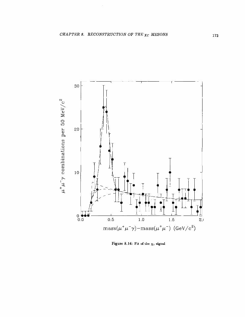
CHAPTER 8. RECONSTRUCTION OF THE xc MESONS
,---------------~,-----------,,-------r ----- --,
30 1-
C\l ()
""-> Q)
~
0 l{)
~ 20 Q)
0.. lf1 ~ 0 .......
+-' eel ~ .......
..0 8 0 ()
r-1
:::t + :::t
10 I I T
I ~~~ ~~ II
-
f l· H · ! ·! c. •• r 1.0 1.5 2.1
Figure 8.14: Fit of the Xc signal
173
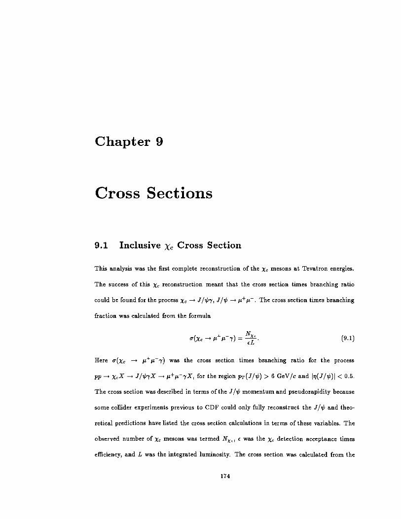
Chapter 9
Cross Sections
9.1 Inclusive Xc Cross Section
This analysis was the first complete reconstruction of the Xc mesons at Tevatron energies.
The success of this Xc reconstruction meant that the cross section times branching ratio
could be found for the process Xc --+ J /1/ry, J /1/J --+ p,+ p,-. The cross section times branching
fraction was calculated from the formula
(9.1)
Here u(xc --+ p,+ IL-r) was the cross section times branching ratio for the process
jip--+ XcX--+ 111/JrX--+ p,+p,-[X, for the region PT(J/1/J) > 6 GeV/c and I77(JN)I < 0.5.
The cross section was described in terms of the J /1/J momentum and pseudorapidity because
some collider experiments previous to CDF could only fully reconstruct the J /1/J and theo-
retical predictions have listed the cross section calculations in terms of these variables. The
observed number of Xc mesons was termed Nxc> E was the Xc detection acceptance times
efficiency, and L was the integrated luminosity. The cross section was calculated from the
174
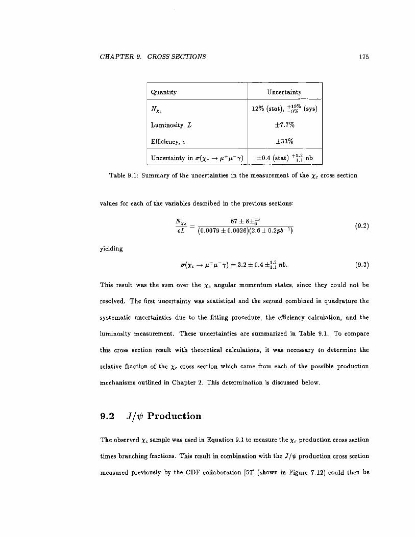
CHAPTER 9. CROSS SECTIONS 175
Quantity Uncertainty
NXc 12% (stat), ~!'t}," (sys)
Luminosity, L ±7.7%
Efficiency, E ±33%
Uncertainty in u(xc -+ 11-+ 11-- 'Y) ±0.4 (stat) ~ti nb
Table 9.1: Summary of the uncertainties in the measurement of the Xc cross section
values for each of the variables described in the previous sections:
NXc __________ 6_7_±~8~±~~~3------~ EL (0.0079 ± 0.0026)(2.6 ± 0.2pb- 1)
(9.2)
yielding
u(xc -+ 11-+ 11-- 'Y) = 3.2 ± 0.4 ±U nb. (9.3)
This result was the sum over the Xc angular momentum states, smce they could not be
resolved. The first uncertainty was statistical and the second combined in quadrature the
systematic uncertainties due to the fitting procedure, the efficiency calculation, and the
luminosity measurement. These uncertainties are summarized in Table 9.1. To compare
this cross section result with theoretical calculations, it was necessary to determine the
relative fraction of the Xc cross section which came from each of the possible production
mechanisms outlined in Chapter 2. This determination is discussed below.
9.2 J /'1/J Production
The observed Xc sample was used in Equation 9.1 to measure the Xc production cross section
times branching fractions. This result in combination with the J /1/J production cross section
measured previously by the CDF collaboration [57] (shown in Figure 7.12) could then be
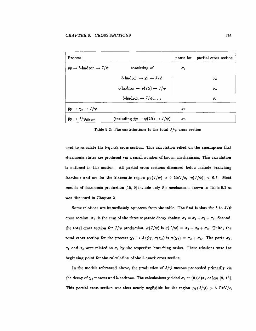
CHAPTER 9. CROSS SECTIONS 176
Process name for partial cross section
frp--+ b-hadron --+ J I..P consisting of 0"1
b-hadron --+ Xc --+ J I..P O"a
b-hadron --+ ,P(2S) --+ J N O"b
b-hadron --+ J 11/Jdirect O"c
pP --+ Xc --+ J N 0"2
pP--+ J 11/Jdirect (including j)p --+ ,P(2S) --+ J N) 0"3
Table 9.2: The contributions to the total J I..P cross section
used to calculate the b-quark cross section. This calculation relied on the assumption that
charmonia states are produced via a small number of known mechanisms. This calculation
is outlined in this section. All partial cross sections discussed below include branching
fractions and are for the kinematic region PT(Jj..p) > 6 GeVIc, I11{JN)I < 0.5. Most
models of charmonia production [15, 9] include only the mechanisms shown in Table 9.2 as
was discussed in Chapter 2.
Some relations are immediately apparent from the table. The first is that the b to J I..P
cross section, o-1, is the sum of the three separate decay chains: 0"1 = O"a + O"b + O"c. Second,
the total cross section for J I ,P production, u( J I ,P) is u( J I ,P) = o-1 + o-2 + 0"3. Third, the
total cross section for the process Xc --+ J I ..P'Y, u(xc) is u(xc) = 0"2 + O" a. The parts O" a,
O"b and u c were related to o-1 by the respective branching ratios. These relations were the
beginning point for the calculation of the b-quark cross section.
In the models referenced above, the production of J I..P mesons proceeded primarily via
the decay of Xc mesons and b-hadrons. The calculations yielded 0"3 ~ (O.OS)o-2 or less [9, 16].
This partial cross section was thus nearly negligible for the region PT ( J I ,P) > 6 Ge VIc,
CHAPTER 9. CROSS SECTIONS 177
Constraint
u(xc) = u2 + Ua = 3.2 ± 1.2 nb this analysis
u(J N) = u1 + u2 + u3 = 6.88 ± 1.11 nb Reference [57]
ua/ul = rx = 0.15 ± 0.05 Equation 2.8
Table 9.3: Constraints on the relationships between the partial J /'1/J cross sections.
117( J /'1/J) I < 0.5 at Tevatron energies. For lower transverse momenta, such would not be the
case, since the direct cross section has a steeply falling spectrum with PT and will be more
significant for lower PT ( J /'1/J). The constraints in the partial cross sections are summarized
in Table 9.3. The = signs in the table signify experimental measurements, while the "" signs
signify assumptions from theoretical models. Solving for u 1 and u 2 yields
(9.4)
and
(9.5)
The results for u1 and u2 for different assumptions for rdir are listed in Table 9.4.
At this point the assumption for the fraction of the J /'1/J cross section from b-decay used
in the efficiency determination in Section 7.3 could be checked. The fraction is defined as
/b = ui/ u( J N) and the results from this section yield
.t 0"! 4.3 ± 1.4 Jbc:=. u(JN) = 6_88 ±1.1 =0.63±0.17 (9.6)
where is should be noted that some of the uncertainty is correlated. The value used for the
efficiency determination was /b = 0.63, which is consistent with Equation 9.6.
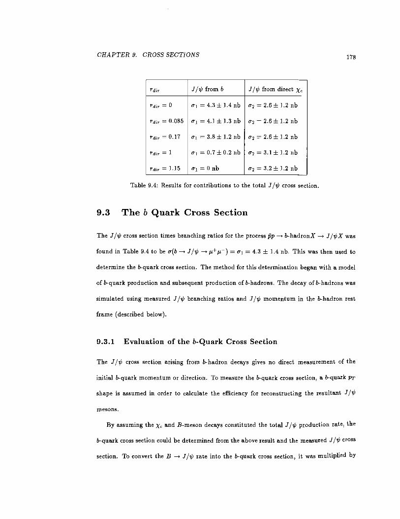
CHAPTER 9. CROSS SECTIONS 178
Tdir JN from b J /1/J from direct Xc
Tdir = 0 o-1 = 4.3 ± 1.4 nb o-2 = 2.6 ± 1.2 nb
Tdir = 0.085 o-1 = 4.1 ± 1.3 nb o-2 = 2.6 ± 1.2 nb
Tdir = 0.17 o-1 = 3.8 ± 1.2 nb o-2 = 2.6 ± 1.2 nb
Tdir = 1 o-1 = 0.7 ± 0.2 nb o-2 = 3.1 ± 1.2 nb
Tdir = 1.15 o-1 = 0 nb o-2 = 3.2 ± 1.2 nb
Table 9.4: Results for contributions to the total J /1/J cross section.
9.3 The b Quark Cross Section
The J /1/J cross section times branching ratios for the process pP--+ b-hadronX --+ J j,PX was
found in Table 9.4 to be o-(b--+ J /1/J --+ 1-L+ 1-L-) = o-1 = 4.3 ± 1.4 nb. This was then used to
determine the b-quark cross section. The method for this determination began with a model
of b-quark production and subsequent production of b-hadrons. The decay of b-hadrons was
simulated using measured J /1/J branching ratios and J /1/J momentum in the b-hadron rest
frame (described below).
9.3.1 Evaluation of the b-Quark Cross Section
The J /1/J cross section arising from b-hadron decays gives no direct measurement of the
initial b-quark momentum or direction. To measure the b-quark cross section, a b-quark PT
shape is assumed in order to calculate the efficiency for reconstructing the resultant J /1/J
mesons.
By assuming the Xc and B-meson decays constituted the total J /1/J production rate, the
b-quark cross section could be determined from the above result and the measured J /1/J cross
section. To convert the B --+ J /1/J rate into the b-quark cross section, it was multiplied by
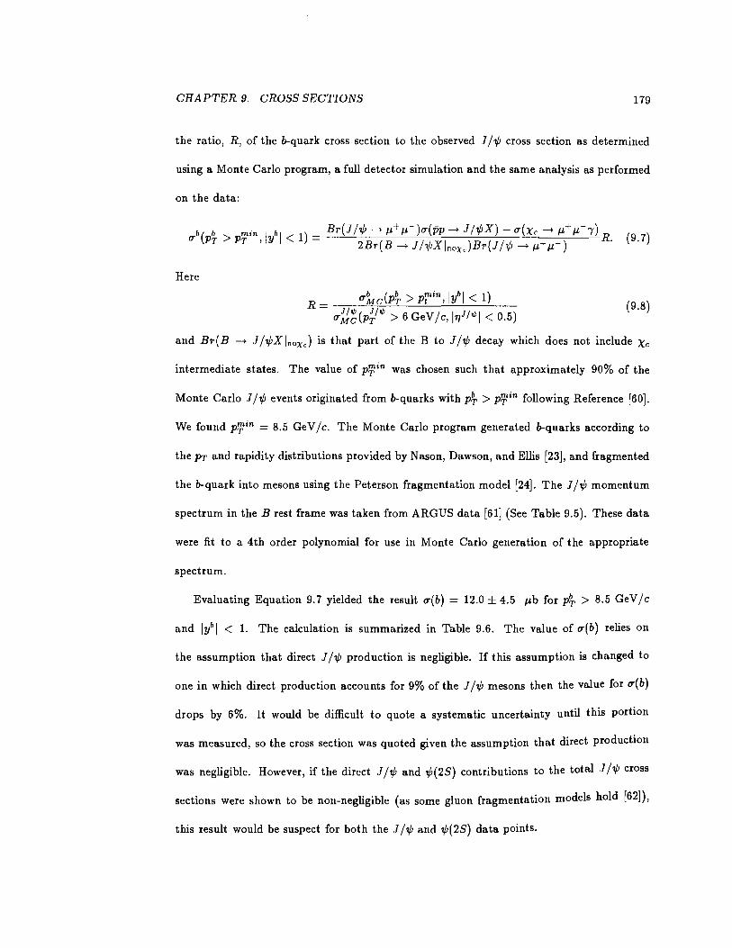
CHAPTER 9. CROSS SECTIONS 179
the ratio, R, of the b-quark cross section to the observed I /1/J cross section as determined
using a Monte Carlo program, a full detector simulation and the same analysis as performed
on the data:
(9.7)
Here
R = O"~c(p~ > Pr'in, lifl < 1) O":J2(P~It/J > 6 GeV jc, l111 /t/JI < 0.5)
(9.8)
and Br(B -+ I /1/JXInoxJ is that part of the B to IN decay which does not include Xc
intermediate states. The value of Prin was chosen such that approximately 90% of the
Monte Carlo J /1/J events originated from b-quarks with p~ > Prin following Reference [60].
We found Prin = 8.5 GeV /c. The Monte Carlo program generated b-quarks according to
the PT and rapidity distributions provided by Nason, Dawson, and Ellis [23], and fragmented
the b-quark into mesons using the Peterson fragmentation model [24]. The J /1/J momentum
spectrum in the Brest frame was taken from ARGUS data [61] (See Table 9.5). These data
were fit to a 4th order polynomial for use in Monte Carlo generation of the appropriate
spectrum.
Evaluating Equation 9. 7 yielded the result O"(b) = 12.0 ± 4.5 ttb for p~ > 8.5 GeV jc
and IYbl < 1. The calculation is summarized in Table 9.6. The value of O"(b) relies on
the assumption that direct J /1/J production is negligible. If this assumption is changed to
one in which direct production accounts for 9% of the J /1/J mesons then the value for O'(b)
drops by 6%. It would be difficult to quote a systematic uncertainty until this portion
was measured, so the cross section was quoted given the assumption that direct production
was negligible. However, if the direct J /1/J and 1/J(2S) contributions to the total I /1/J cross
sections were shown to be non-negligible (as some gluon fragmentation models hold [62]),
this result would be suspect for both the J /1/J and 1/J(2S) data points.
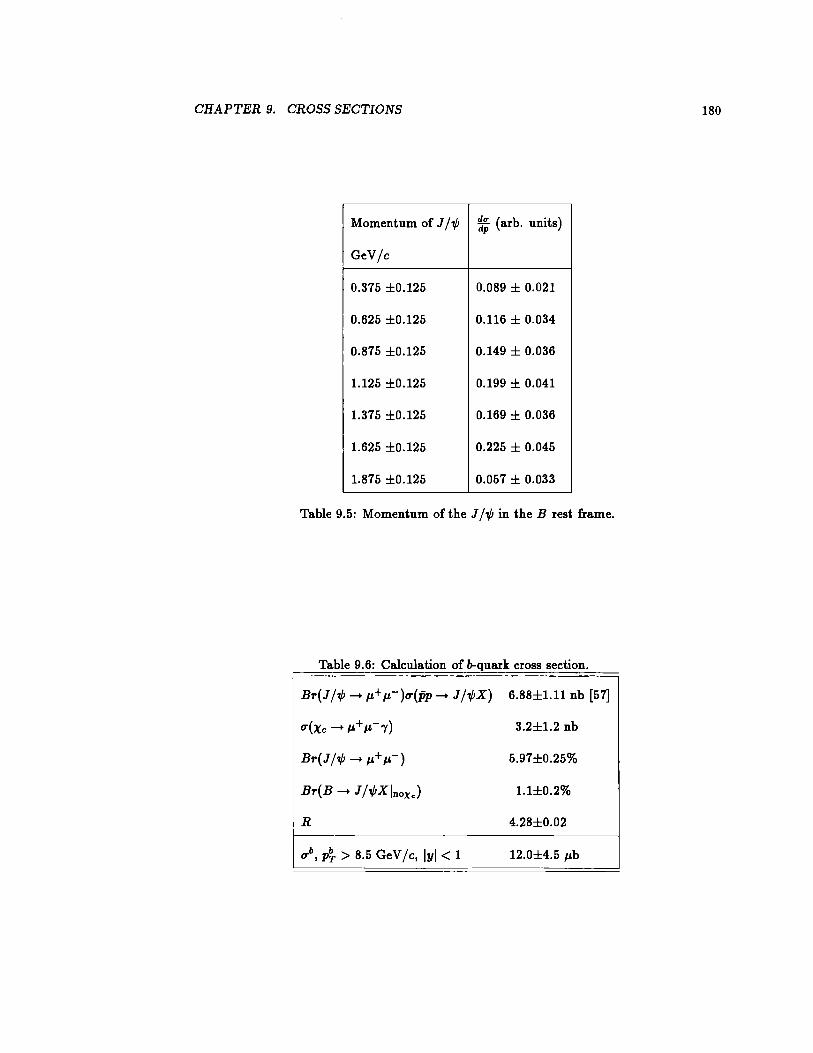
CHAPTER 9. CROSS SECTIONS 180
Momentum of J j.,P ~; (arb. units)
GeV/c
0.375 ±0.125 0.089 ± 0.021
0.625 ±0.125 0.116 ± 0.034
0.875 ±0.125 0.149 ± 0.036
1.125 ±0.125 0.199 ± 0.041
1.375 ±0.125 0.169 ± 0.036
1.625 ±0.125 0.225 ± 0.045
1.875 ±0.125 0.057 ± 0.033
Table 9.5: Momentum of the J j.,P in the B rest frame.
Table 9.6: Calculation of b-quark cross section.
Br(JN-+ JL+JL-)u(jjp-+ JNX) 6.88±1.11 nb [57]
u(xc-+ JL+JL-'Y) 3.2±1.2 nb
Br(JN-+ JL+JL-) 5.97±0.25%
Br(B-+ J NXInoxJ 1.1±0.2%
R 4.28±0.02
ub, p~ > 8.5 Ge V / c, IYI < 1 12.0±4.5 JLb

Chapter 10
Conclusions
The purpose of this work was to perform a measurement of the Xc meson cross section
at j)p interactions, and compare this to the cross section calculated within the theoretical
framework outlined in the first two chapters. The b-quark cross section was also determined
as a by-product, due to the shared J / 1/J possible in the final state of Xc and b-hadron decays.
In this chapter, the measurements are compared to the calculations, and conclusions on the
efficacy of the predictions are arrived at. First, the Xc cross section (central to this work) is
examined below, then the b-quark cross section is briefly discussed.
10.1 Xc prod net ion theory
The portion of Xc meson production cross section not arising from b-hadron decays (decaying
into JN mesons with PT(JN) > 6 GeV/c and I11{JN)I < 0.5) was determined from
Table 9.4 to be 2.6 ± 1.2 nb. The theoretical estimate of this same cross section, assuming
a K-factor of 2.0 (as at lower energies [9, 20]) and Q2 = (p} + m~)/4, was 2.8 nb, in
agreement with the actual measurement. If the assumptions for the value of Q2 was changed
181

CHAPTER 10. CONCLUSIONS 182
to (p} + m~), the estimate was lowered to 1.4 nb, still within the uncertainties of the
measurement. Within the precision of the measurement performed in this analysis, the
model proved useful for describing the production process. However, some concerns with
the model still exist. Some of these are discussed below.
A K-factor of 2.0 may indicate that each additional term (an order higher in a.) may
be of a similar magnitude to the entire cross section. Thus, the model would be outside a
regime where perturbative calculations could be trusted, and the ability of the calculation
to arrive at the measured value may have been serendipitous, or the higher order terms
could significantly alter the expected PT and 11 shapes of the production cross section.
Another concern is the value chosen for Q 2 • A naive approach might indeed be to
choose the approximate energy of the Xc divided by the number of initial partons as an
approximate magnitude for IQI. But the possibility exists that the dividing factor of 4 in
Q 2 = (p} + m~)/4 is indicative of a problem with the scale A used in the a. calculation. In
addition, some choices of Q2 have a different PT dependence, which would again alter the
calculated PT spectrum of Xc meson production.
Additionally, the theoretical calculations give direct J j.,P production estimates signifi-
cantly less than Xc or b-hadron to J /1/J processes. Although the direct Xc cross section does
not depend significantly upon this ratio (being bounded from 2.6 ± 1.2 to 3.2 ± 1.2 nb as
seen in Table 9.4), at some future level of precision for measurements of this cross section
this might pose a real concern.
As it stands, however, no major modifications of the framework for the calculation of Xc
mesons is now required. A QCD perturbative approach with reasonable assumptions has
resulted in a match between calculations and Xc mesons observed at vs = 1.8 TeV. This
shows the success and usefulness of the model.
CHAPTER 10. CONCLUSIONS 183
10.2 b-quark production
The b-quark cross section arrived at in this work (through the decay into final states con-
taining J N) was
u(b, p~ > 8.5GeV/c, IYbl < 1) = 12.0 ± 4.51J.b. (10.1)
Other methods of estimating the b-quark cross section at CDF have also been employed,
including from '¢(2S) final states [57], inclusive lepton production (both electrons [63] and
muons [64]) as well as full reconstruction of B mesons [11, 12]. These results are summarized
in Figure 10.1, which also includes the a~ calculation for the b-quark cross section as a
function of the minimum b-quark PT· The value obtained here (in Equation 10.1) was
labelled the J /1/IX point, since it was arrived at by the J /'¢ production subtracting out
Xc mechanisms. This is consistent with the b-quark cross section estimated from '¢(25)
production [57]. Both of these methods assume that direct production of J N and '¢(25)
are negligible. The other points on the curve do not rely on this assumption. It is useful
to note that the calculated curve lies below the measurements. This poses a challenge to
physicists, to find a variation to the model (possibly a new choice for Q2 , higher order
calculations, or a new set of structure functions) to describe the measurements. The general
shape is as expected, although more precise quantitative tests need to be made. The state
of the model may not change much before it is as useful describing b-quark production as it
is describing Xc meson production.
10.3 Summary
The production of Xc mesons was relatively well understood within the framework of per-
turbative QCD, a part of the standard model of particles and interactions. The calculations
from this model are consistent with observations. While refinements continue to be made
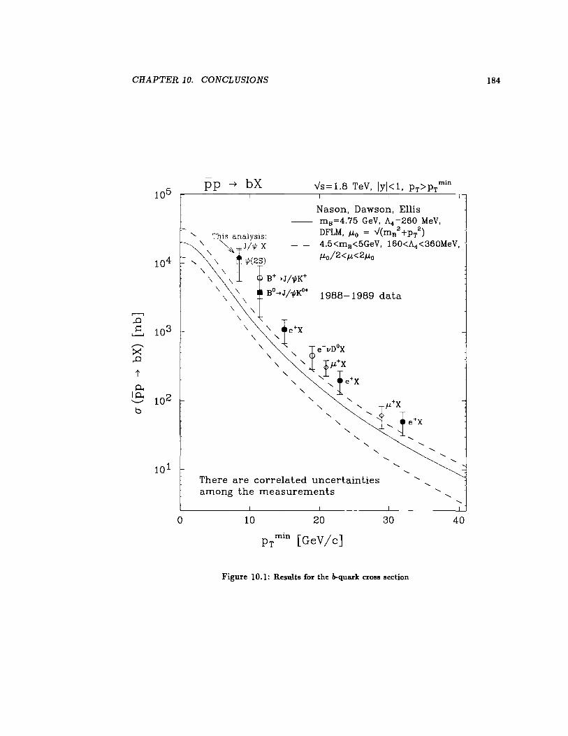
CHAPTER 10. CONCLUSIONS
b
101
0
pp ~ bX
There are correlated
Ys=1.8 TeV, IYI<l, Pr>Prmin
Nason, Dawson, Ellis rn8 =4.75 GeV, A4 =260 MeV, DFLM, J.l-o = v'(rnB 2 +Pr 2) 4.5<rn8 <5GeV, 160<A4 <360MeV, J.Lo/2<J.L<2J.Lo
' ' ' ' ' ' ' ' ' uncertainties ' ' among the measurements '
10 20 30 40
PT min [ Ge V / C]
Figure 10.1: Results for the b-quark cross section
184

CHAPTER 10. CONCLUSIONS 185
to the models, QCD remains a useful map of strong interactions.

Bibliography
[1] See, for example, Genesis in Space and Time and No Final Conflict, Francis Scha-
effer, In "The Complete Works of Francis A. Schaeffer", Volume 2, p.3-148 Second
Edition, 1986, Crossway Books, Westchester, Illinois, or, "Foundations of Christian
Scholarship", Gary North, editor, 1979, Ross House Books, Vallecito, California.
[2] "The Structure of Scientific Revolutions", Thomas S. Kuhn, 1962, The University of
Chicago Press, Chicago, Illinois.
[3] W. Weinberg, Physical Review Letters 19 1264 (1967), A. Salam, Elementary Particle
Theory: Relativistic Groups and Analyticity (8th Nobel Symposium) 367 (1968).
[4] Particle Data Group, K. Hidasa et al., Review of Particle Properties Physical Review,
D 45, 11 Part II (1992)
[5] J.-E. Augustin, et al., Physical Review Letters 33 1406-1408 (1974).
J.J. Aubert, et al., Physical Review Letters 33 1404-1406 (1974).
G.S. Abrams, et al., Physical Review Letters 33 1453-1455 (1974).
[6] T. Appelquist, et al., Physical Review Letters 34 365-369 (1975).
E. Eichten, et al., Physical Review Letters 34 369-372 (1975).
186
BIBLIOGRAPHY 187
(7] S.W. Herb, et al., Physical Review Letters 39 252-255 (1977).
W.R. Innes, et al., Physical Review Letters 39 1240-1242,1640(E) (1977).
(8] Examples of the use of spectroscopic variables in atomic phenomena are listed in many
textbooks, for example "Elementary Atomic Structure", G.K. Woodgate, 1980, Oxford
University Press, Oxford.
(9] E.W.N. Glover, A.D. Martin, W.J. Stirling, Z. Phys. C 38, 473-478 (1988).
(10] E.W.N. Glover, F. Halzen, A.D. Martin Physics Letters B 185, 441-445 (1987).
(11] F. Abe, et al., Physical Review Letters, 68 3403-3407 (1992).
(12] A Measurement of the B Quark and Neutral B meson Production Cross Sections in
Proton-Antiproton Collisions at a Center of Mass Energy of 1.8 TeVBy Steve Vejcik,
III (The Johns Hopkins University), UMI-93-13448-mc, Aug 1992. 175pp. Ph.D.Thesis.
(13] R. Baier, R. Rucki, Z. Phys. C 19, 251-266 (1983).
(14] Z. Kunszt, et al., Physical Review D 21 733 (1980).
(15] M Mangano, INFN Report No. IFUP-TH 2/93, 1993 (to be published).
(16] Nigel Glover, private communication.
(17] R. Baier, R. Rucki, Nuclear Physics B 208 381-396 (1982).
(18] B. Humpert, Physics Letters B 184 105-107 (1987).
(19] R. Gastmans, W. Troost, Tai Tsun Wu, Physics Letters B 184 257-260 (1987).
(20] A.G. Clark, et al., Nuclear Physics B 142, 29 (1978),
C. Kourkoumelis, et al., Physics Letters 81 B, 405 (1979).
C. Kourkoumelis, et al., Physics Letters 91 B, 481 (1980).
BIBLIOGRAPHY 188
[21] T.A. Armstrong, et al., Nuclear Physics B 373 35-54 (1992).
[22] A. Martin, R. Roberts, J. Stirling, RAL-92-021, DTP/92/16 (1992).
[23] P. Nason, S. Dawson, R.K. Ellis, Nuclear Physics B 303 607 (1988), Nuclear Physics
B 327 49 (1989), Nuclear Physics B 335 260 (1990).
[24] C. Peterson, D. Schlatter, I. Schmitt, P. Zerwas, Physical Review D 27 105 (1983).
[25] D. Bortoletto, et al., Physical Review D 37 1719 (1988).
[26] B. Gittelman, in Proceedings of the Vancouver Meeting {1991 DPF Meeting) (World
Scientific, Singapore, 1991), p.l81.
[27] L.M. Lederman, Scientific American 264 No.3 26-33 (1991).
[28] F. Abe, et al., Nuclear Instruments and Methods A 271 387-403 (1988).
[29] S. Mori, et al., Nuclear Instruments and Methods A 238 18-34 (1985).
[30] T. Kamon, et al., Nuclear Instruments and Methods 213 261 (1983).
[31] K. Yasuoka, et al., Nuclear Instruments and Methods A 267 315-329 (1988)
[32] R.G. Wagner, et al., Nuclear Instruments and Methods A 267 330-350 (1988)
[33] D. Amidei et al., Nucl. lnstrum. Methods A 267, 51 (1988).
[34] T. Carroll et al., Nucl. Instrum. Methods A 263, 199 (1988).
[35] G. Ascoli et al., Nucl. Instrum. Methods A 267, 272 (1988).
[36] A. Gauthier, CDF internal note 937, 1989 (unpublished.)
[37] R. Hughes, et al., CDF internal notes 1625 and 1385, 1991 (unpublished).
BIBLIOGRAPHY 189
[38] G. W. Foster et al., Nucl. Instrum. Methods A 269, 93 (1988).
[39] Rick Snider, private communication
[40] Peter Berge, private communication.
[41] F. Abe et al., Physical Review D, 43, 2070 (1991).
[42] F. Abe et al., Physical Review Letters, 68, 3403 (1992).
[43] F. Bedeschi et al., Nucl. Instrum. Methods A 268, 50 (1988).
[44] R. Harris, CDF internal note 1329, (1991). See also F. Abe et al., Fermilab Report No.
Fermilab-PUB-92/01-E, 1992.
[45] F. Abe et al., Physical Review Letters, 68, 2734 (1992).
[46] K. Yasuoka et al., Nucl. Instrum. Methods A 267, 315 (1988).
[47] R. Wagner et al., Nucl. lnstrum. Methods A 267, 330 (1988).
[48] F. Abe et al. Physical Review Letters, 63, 720 (1989).
[49] M. Bozzo et al., Phys. Lett. 147B, 392 (1984).
[50] F. Abe et al., Physical Review D 44, 29 (1991).
[51] L. Balka, et al., Nuclear Instruments and Methods A267 272-279 (1988).
[52] CDF internal note 1436 (unpublished).
[53] CDF internal note 1435 (unpublished).
[54] CDF internal note 1432 (unpublished).
[55] F. Paige, S.D. Protopopescu, ISAJET Monte Carlo version 6.36, BNL Report No.
BNL38034, 1986 (unpublished).
BIBLIOGRAPHY 190
[56] W. Wester, private communication.
[57] F. Abe, et al., Physical Review Letters, 69 3704-3708 (1992).
[58] D. Frei, CDF internal note 1430, 1991 (unpublished).
[59] C. Boswell, Minutes of the CDF dilepton meeting, January 23, 1992 (unpublished).
[60] N. Ellis, A. Kernan, Physics Reports 195 23-125 (1990).
[61] H. Schroder, in 25th International Conference on High Energy Physics Singapore, Au-
gust 2-8, 1990, K.K. Phua and Y. Yamaguchi, editors, pp.846-849 (Volume II), pub-
lished by South East Asia Theoretical Physics Association and the Physical Society of
Japan, Distributed by World Scientific Publishing, Singapore.
[62] E. Braaten and T.C. Yuan, preprint NUHEP-TH-92-23 (UCD-92-25), (revised version)
February 1993.
[63] F. Abe, et al., Physical Review Letters 71, 500-504 (1993).
[64] F. Abe, et al., FERMILAB-PUB-93-145-E, June 1993, submitted to Physical Review
Letters.
Christopher Mark Boswell
BIRTHPLACE:
EDUCATION:
EXPERIENCE:
B.S.: Seattle Pacific University, 1986. M.A.: The Johns Hopkins University, 1988.
The Johns Hopkins University, 1993. Ph.D:
Experimental High Energy Physics
Postgraduate Reasearch Scientist, University of California, Riverside Silicon Detector Group,
DO detector at FN AL, April 1993 to present.
Research Assistant, The Johns Hopkins University, Silicon Vertex detector (SVX) group,
CDF detector at FNAL, March 1989 to April 1993.
Silicon Strip Vertex Detector (SSVD) group, Mark-II detector at SLAC, July 1988 to March 1989.


![Proton–proton and proton–antiproton differential elastic …...Elastic scattering and diffraction dissociation Measurement) at the LHC Collaboration [30–35]. Furthermore, different](https://img.pdfslide.us/doc/110x75/60e2a38bc9ae1d4e2f17cd71/protonaproton-and-protonaantiproton-differential-elastic-elastic-scattering.jpg)