Efficient frontiers for electricity procurement by an LDC with multiple purchase options

Chi-Keung Wooa,b,*, Ira Horowitzc,d, Arne Olsona, Brian Horiia, Carmen Baskettea

Abstract

In meeting its retail sales obligations, management of a local distribution company (LDC) must

determine the extent to which it should rely on spot markets, forward contracts, and the

increasingly popular long-term tolling agreements under which it pays a fee to reserve generator

capacity. We address these issues by solving a mathematical programming model to derive the

efficient frontier that summarizes the optimal tradeoffs available to the LDC between

procurement risk and expected cost. To illustrate the approach, we estimate the expected

procurement costs and associated variances that proxy for risk through a spot-price regression for

the spot-purchase alternative and a variable-cost regression for the tolling-agreement alternative.

The estimated regressions yield the estimates required to determine the efficient frontier. We

develop several such frontiers under alternative assumptions as to the forward-contract price and

the tolling agreement’s capacity payment, and discuss the implications of our results for LDC

management.

Keywords: Efficient frontier, Cross hedging; Forward contracts; Tolling agreements; Partial-

adjustment model

a. Energy and Environmental Economics, Inc., 353 Sacramento Street, Suite 1700, San

Francisco, CA 94111 USA

b. Hong Kong Energy Studies Centre, Hong Kong Baptist University, Hong Kong

c. Decision and Information Sciences, Warrington College of Business Administration,

University of Florida, Gainesville, FL 32611-7169

d. Information and Decision Systems, College of Business Administration, San Diego State

University, San Diego, CA 92182-8221

* Corresponding author. Tel: +1-415-391-5100; Fax: +1-415-391-6500; Email address:

ck@ethree.com

1

1. Introduction

A concomitant of deregulation and related market reforms in the electricity industry in

the United States has been the emergence of wholesale electricity spot markets for which highly

volatile prices that are at best amenable to imperfect forecasts are the norm. The price volatility

and forecast imperfection have two principal sources: (1) the random demand surges that the

buyers, notably local distribution companies (LDCs) that must procure electricity to meet

customer demand in real time, have to deal with in the face of the generators’ upward-sloping

electricity supply curve; and (2) random capacity shortages due to unexpected generation or

transmission outages that shift the supply curve upwards along a downward-sloping and inelastic

electricity demand curve [1 – 3]. Analogous random changes in the price of natural gas, which is

both an input into the electricity generation process as well as a competitive energy source, can

further exacerbate the electricity spot-price volatility [4 – 5]. If unmitigated, such price volatility

can financially ruin an LDC with its obligation to serve at regulated rates unresponsive to

wholesale spot market prices. A dramatic case in point is the April 6, 2001 bankruptcy of Pacific

Gas and Electric Company (PG&E), one of the largest LDCs in the United States [6 – 10]. Both

state and federal governments now endorse the important role of risk management in the energy

business [11 – 12].

Recent analyses of an LDC’s management of electricity-procurement cost and risk have

focused on two procurement alternatives: spot-market purchases and fixed-price forward-

contract purchases [13 – 15]. The latter facilitate risk management and mitigate potential market-

power abuses by generators, because they reduce an LDC’s dependence on the spot markets [16].

LDC management, however, may be reluctant to enter into a long-term forward contract if the

2

LDC’s regulator - and the industry remains subject to partial regulation - can engage in an after-

the-fact prudence review that might result in full cost recovery being disallowed [9; 17].

To be sure, legislative actions can minimize the need for and use of after-the-fact

prudence reviews. For example, California Assembly Bill (AB) 57 that became law on

September 25 2002 directs “the Public Utilities Commission …. to review each electrical

corporation’s procurement plan in a manner that assures creation of a diversified procurement

portfolio, assures just and reasonable electricity rates, provides certainty to the electrical

corporation in order to enhance its financial stability and credit worthiness, and eliminates the

need, with certain exceptions, for after-the-fact reasonableness reviews of an electrical

corporation’s prospective electricity procurement performed consistent with an approved

procurement plan” (SECTION 1(c)).

On October 24, 2002, the California Public Utilities Commission (CPUC) issued

Decision 02-10-062, which implements AB57. The Decision requires the three large utilities,

PG&E, Southern California Edison (SCE) and San Diego Gas and Electric (SDGE), to submit

procurement plans for the CPUC’s approval. A critical element of such plans is the choice

among alternative electricity-procurement options. That is, in meeting its down-the-road

electricity requirements: To what extent should the LDC rely on spot markets? To what extent

should it rely on forward contracts? And to what extent should it rely on the increasingly popular

long-term tolling agreements under which the LDC pays a generator a fee to, in effect, reserve

some of the generator’s capacity?

We address these issues by first solving the mathematical programming model from

which one derives the efficient frontier that summarizes the optimal tradeoffs available to LDC

management between procurement risk and expected cost, when it can diversify its electricity

3

purchases through electricity spot markets, fixed-price forward contracts, and tolling agreements.

We then put empirical meat on these theoretical bones via an application in which we estimate

expected procurement costs and the associated variances that proxy for risk. The estimation

entails a spot-price regression for the spot-purchase alternative and a variable-cost regression for

the tolling-agreement alternative. The estimated regressions yield the parameter estimates

required to determine the efficient frontier. We develop several such frontiers under alternative

assumptions as to the forward-contract price and the tolling agreement’s capacity payment, and

discuss the implications of our results for LDC management.

2. The efficient frontier

Consider an LDC that requires a flat power block of a given megawatt (MW) size to be

delivered at 100%, 24 hours a day, seven days a week. The LDC has three procurement

alternatives for buying the base-load power that will enable it to meet its resale obligation of

serving its retail end-users:

(1) Spot-market purchases from a local hub, such as Mid-Columbia (Mid-C) in the state of

Washington. Complete reliance on this alternative, however, exposes the LDC to the risk

entailed in potentially volatile spot prices.

(2) A fixed-price forward contract offered by a generator such as Calpine or by a marketer/trader

such as Morgan Stanley. The contract obligates the seller to physically deliver, and the LDC

to accept, power at a fixed price. Relatively less risk verse than the buyer, the seller absorbs

the spot-price risk and may charge the LDC a risk premium to ensure the forward contract’s

profitability [18 – 19].

(3) A tolling agreement offered by a generator. The agreement gives the LDC the right, but not

the obligation, to dispatch a generation unit specified by the agreement. The LDC pays the

4

generator a fixed per kilowatt (kW) payment for having the capacity available at an agreed

fuel conversion rate (i.e., the heat rate in British thermal units (Btu) per kilowatt-hour

(kWh)). The LDC supplies the fuel used by the generator, typically natural gas, and absorbs

the fuel price risk. Since a generation unit’s non-fuel variable cost is negligible, the LDC’s

least-cost operating decision is to dispatch the leased capacity whenever the per megawatt

hour (MWh) fuel cost is less than the electricity spot price in $/MWh. The payment per kW

is therefore the call-option value of a one kW capacity with a specific heat rate [20 – 21]. The

capacity payment is equivalent to a fixed MWh payment for each MWh obtained by the

LDC, irrespective of whether that MWh comes from the generator or the spot market.

Specifically, the capacity charge per MWh is the capacity payment per kW-month multiplied

by 1,000 and divided by the number of hours (e.g., 744 for January) in the month. Least-cost

dispatch decisions by the LDC always result in a variable cost per MWh that is lower and

less volatile than the spot price, except under the highly unlikely scenario in which the spot

price never exceeds the per MWh fuel cost of the tolling agreement.

Denote the average cost and variance per MWh of spot-market purchases by µ1 and σ12,

respectively, with µ2 and σ22, and µ3 and σ3

2, denoting the average costs and variances for a

tolling agreement and a fixed-price forward contract, respectively; σij denotes the covariance

between the purchase costs in the ith option and those in the jth. The average cost for the tolling

agreement, µ2, is the fixed capacity payment per MWh plus the average variable cost per MWh.

Hence the associated cost variance, σ22, is the variance of the variable cost per MWh. The latter

is necessarily less than σ12, because it is only computed for Min[spot price, per MWh fuel cost].

The forward contract’s average cost, µ3, is its fixed price and therefore the variance is σ32 = 0.

Inasmuch as σ12 > σ2

2 > σ32 = 0, we expect and assume µ1 < µ2 < µ3; otherwise a risk-averse

5

management would be inclined to either put all its eggs in the risk-free forward-contract basket

when that option is available, or, failing that, reduce exposure to the risk of upward-spiraling

spot-market prices via a tolling agreement for which µ1 > µ2.

And we do indeed assume the LDC management to be risk averse, as well as budget

conscious in the sense of setting an upper bound on its expected procurement cost. Following

Markowitz [22] and Woo et al. [14], management will seek to determine weights of w1 ≥ 0, w2 ≥

0, and w3 ≥ 0, for the amount of electricity procured via the spot market, a tolling agreement, and

a forward contract. The optimal weights will minimize the variance of its procurement portfolio,

subject to its expected procurement-cost constraint. The non-negativity condition on the weights,

which sum to unity, is applied to preclude short selling and the excessive risk taking that such

implies. Further, since there is a fixed purchase quantity, minimizing the procurement-cost

variance per MWh of a portfolio comprising the three electricity procurement alternatives is

equivalent to minimizing the total procurement-cost variance.

Let l = [1, 1, 1]T, 0 = [0, 0, 0]T, wT = [w1, w2, w3], and µT = [µ1, µ2, µ3], and denote by Ω

the positive-definite variance-covariance matrix for the three purchase alternatives. Then, the

cost variance of the procurement portfolio is σ2 = wTΩw and its expected cost is µ = wTµ, where

wTl = 1. Suppose management places an upper bound of M on the expected procurement cost per

MWH that it is willing to incur. Stated formally, management’s optimization problem may be

written:

Minimize σ2 = wTΩw w

Subject to:

wTµ ≤ M

wTl = 1

6

w ≥ 0.

Since Ω is positive definite and the constraints are linear, the optimal solution to the

problem, which can be solved by standard techniques, [22 -23], satisfies the Karoush-Kuhn-

Tucker conditions. With λ ≥ 0 a Lagrange multiplier, and L = σ2 + λ[wTµ – M], an interior

solution satisfies ∂L/∂w = 0 and wTµ = M. It is easily shown that plotting the minimum

procurement-cost variance σ*2 on the vertical axis and the binding cap of M = µ*, the expected

procurement cost that is co-joined to that variance, on the horizontal axis, describes a downward

sloping and strictly convex efficient frontier.

3. An application

3.1 The setting

To show the practicality of the efficient-frontier approach, we consider a hypothetical

LDC housed in the Pacific Northwest. We assume that LDC management employs a

procurement process that entails the following four steps [17]:

(1) Assess the purchase requirements that will meet the LDC’s load obligation;

(2) Assess the procurement alternatives through which the LDC can meet the purchase

requirements;

(3) Issue a request for proposal (RFP) to obtain competitive bids for alternatives that are

not actively traded in wholesale markets;

(4) Evaluate the bids by considering the tradeoffs of the procurement-cost expectations

and cost variances presented by the alternatives, including the default alternative of

purchasing from the spot market.

Under this assumed process, management considers purchasing a flat power block for a

five-year term. The point of delivery is Mid-C. While standard forward contracts are available in

7

the Mid-C market, at present they are only offered for terms up to three years and are only for the

on-peak hours (06:00-22:00, Monday – Saturday), rather than (7x24) delivery. Hence, the LDC

follows steps (2) and (3) by issuing an RFP to potential suppliers to submit competitive bids for

forward contracts and tolling agreements.

The bid submission can be a sealed-bid auction or an internet-based auction [24]. A

forward-contract bid should contain a single fixed-price quote. A tolling-agreement bid should

contain a single quote for the capacity payment per kW-month, and state the generation unit’s

heat rate.

Management then implements step (4), bid evaluation, which requires knowledge of the

available optimal tradeoffs between the procurement-cost expectation and the procurement-cost

variance presented by the bids, and the default alternative of buying from the spot market. This

knowledge is best summarized in an efficient frontier. The LDC management’s risk preferences,

or the tradeoffs they are willing to accept between, in effect, risk and return, would then

determine the optimal point on the frontier [14].

3.2 The spot-price equation and cross hedging

To derive the expected procurement cost and the variance of the spot-purchase

alternative, we focus on two specific markets: the spot market for electricity at Mid-C and that

for natural gas at Henry Hub, which is the most active spot and futures market in North America.

As shown in [15, 18 - 19], LDC management can avail itself of the option to cross hedge

between these two markets. This option is available for four principal reasons.

First, as a basic input in electricity generation, the natural-gas price helps to drive

electricity prices [4, 25]. Second, local natural-gas spot markets, such as Sumas in the Pacific

Northwest, are integrated with Henry Hub [5, 10, 25 - 28]. Third, Henry Hub natural-gas futures

8

contracts currently traded on the New York Mercantile Exchange (NYMEX) are for delivery in

the next 72 months, which is a sufficiently long time period to permit cross hedging the five-year

price/cost risk. Finally, the NYMEX natural-gas futures market is efficient [29].

Suppose, then, that Pt is the Mid-C electricity spot price on some future day t for which

we want to determine the expected procurement cost and that PGt is the currently unknown

Henry Hub natural-gas spot price on that day. Since natural-gas prices help drive electricity

prices, we hypothesize that there is a systematic linear relationship, Pt = α + βPGt, between these

two prices, and that the spot price is also impacted by a normally-distributed random error of εt

that has a zero mean and finite variance of ν2 > 0; or:

Pt = α + βPGt + εt. (1)

Thus, from management’s current perspective Pt is random and volatile because both PGt and εt

are random and potentially volatile.

Cross hedging against the volatility of Pt begins with the current purchase of β MMBtu of

natural-gas futures at a price of PGF =$F/MMBtu for each MWh delivered at Mid-C. Then, on

future day t, the LDC resells the natural gas bought at PGF at the Henry Hub natural-gas spot

price PGt. The net spot price for Mid-C electricity, after allowing for the machinations in the

natural-gas market and substituting equation (7) for Pt, is therefore:

Pnt = Pt - β(PGt – PGF) = α + βPGt + εt - βPGt + βPGF = α + βPGF + εt. (2)

The future net spot price, Pnt, is thus a function of the known price of PGF. Once values have

been determined for α and β, the only uncertainty that remains for management as a result of

having cross-hedged is introduced by the random error. Hence, the variance of ν2 > 0 is the

minimum variance that cannot be eliminated by cross hedging. This represents the

undiversifiable price risk, while β is the minimum-variance hedge ratio [30].

9

The preceding analysis implies that when evaluating the spot-market alternative for

procuring electricity, it is necessary to incorporate the risk-reducing cross-hedging option and to

compute expected procurement costs on the basis of the net spot price, rather than on the spot

price. Thus, rather than being concerned with the determination of the expected spot price and

the spot-price variance, our interest will be in determining the expected net spot price and its

necessarily smaller variance.

3.3 Partial adjustment

When the Mid-C market is in equilibrium, the average equilibrium price on day t, Pte,

will equal the spot price. Hence Pte will also necessarily satisfy spot-price equation (1); or:

Pte = α + βPGt + εt. (3)

Any Mid-C market equilibrium on day t might therefore be disturbed by both the random

changes that occur in the Henry Hub natural-gas market and through the noise factor. The daily

and unobservable market equilibrium price may not, however, adjust instantaneously to those

random shocks. To capture this possibility, we postulate the observed spot-market price

adjustment to be a fraction, γ, of the unobservable required adjustment [31, Chapter 11]. That is:

Pt – Pt-1 = γ(Pte – Pt-1). (4)

Substituting Pte from equation (3) into equation (4) and rearranging terms yields:

Pt = γα + γβPGt + (1 - γ)Pt-1+ γεt. (5)

The latter may be more compactly written as:

Pt = θ + ϕPGt + φPt-1+ ηt. (5a)

Thus, θ = γα, ϕ = γβ, φ = (1 - γ) and ηt = γεt.

Using daily data for the Mid-C electricity spot price and the Henry Hub natural-gas spot

price, we apply the maximum likelihood (ML) method to estimate equation (5a). The use of ML

10

avoids the potential bias caused by the lagged dependent variable as an explanatory variable in a

regression that may have first-order autoregressive (AR(1)) errors. Our choice of estimation

method is partly based on our analysis of natural-gas prices [5], which as shown by equation (3)

are postulated to impact electricity spot prices and hence the variable costs of the tolling

agreement. Whether our chosen estimation method is appropriate is ultimately an empirical

issue. Absent AR(1) errors, ordinary least squares (OLS) estimation will yield consistent and

asymptotically normal estimates. Should the errors turn out to have a higher AR order, one

should use the ML method that would account for such errors. As will be seen in Table 2 below,

our chosen estimation method is appropriate. The estimation will yield:

• (q, g, f), the estimates for coefficients (θ, ϕ, φ)

• r, the estimate for the AR(1) parameter;

• the covariance matrix for the coefficient estimates; and

• the mean-squared-error (MSE) of the daily price regression.

We can then infer, say, a and b, the estimates for α and β, from a = q/(1 – f) and b = g/(1 – f).

3.4 The expected net spot price and its variance

Assuming that no major structural change occurs during the forecast period that might

invalidate our regression results, these results, rather than computer simulation as in [21, 32], can

be used as the basis for computing the expected net spot price and its variance. The approach

thus relies solely on market data and does consider the technical details (e.g., generation plants

and transmission capabilities) that may underlie those data. So long as there are historic spot-

price data for electricity and natural gas for local delivery at the LDC’s service territory, along

with natural-gas futures covering the LDC’s procurement horizon, and such data are indeed

always available in North America, our approach will yield the inputs required for developing

11

the efficient frontiers. Therefore it is a practical and easy-to-implement alternative to the more

exotic formulae proffered elsewhere, for example [21, 33 - 34], whose complicated natures are

likely to deter application by an LDC’s staff, frustrate review by its management, and

subsequently invite a regulator’s disapproval.

The simplest tack for management to take at this point would be to accept

a and b as the actual values of α and β rather than merely their ML point estimates. To capture

the uncertainty about the still unknown α and β when computing the expected net spot price and

its variance, however, which will be accomplished through equation (2), suppose management

adopts an empirical Bayes approach [35 – 36]. The approach has survived the test of time [37 -

39], both because it permits a very useful probabilistic interpretation of sample results in the

subjective Bayesian context, and because it becomes especially useful when “data are generated

by repeated execution of the same type of random experiment” [39, p. 1].

In particular, we rely on a “somewhat broader interpretation of the term ‘empirical

Bayes’ than is implied in the typical EB sampling scheme”, wherein the “parameter ω of a prior

distribution … is replaced by any estimate derived from observed data…” [39, p. 14]. In the

present context, LDC management uses the estimated regression results from equation (5a) as the

basis for formulating a set of probability judgments about α and β of spot-price equation (1). In

particular, management behaves “as if” the computed standard error of estimate from equation

(5a) permits the derivation of ν2. It also formulates probability judgments about α and β that are

summarized in normal distributions with means of a and b, and assigned variances of sa2 and sb

2.

The covariance between α and β is set at sab. The two variances and the covariance are linear

approximations derived from the estimated standard errors and covariance that are computed

when equation (5a) is estimated. The approximations use a well-known formula [40, p. 181] for

12

the mean and variance of Z = g(X, Y), where X and Y are random variables. We remark, en

passant, that we could have used a Bayesian approach in the initial specification of equation (1)

and then incorporated equation (4), which is not a statistical statement, but we elected not to do

so as we felt it might be a distraction at that point from the general development of the model in

a more traditional mode.

Denote by PGFk the fixed current Henry Hub natural-gas futures price for month k that

encompasses day t and denote by E the expectation operator. The Mid-C electricity net spot price

on day t in that month will be determined by equation (2). Hence the expected net spot price will

be given by:

E[Pnkt] = E[α] + E[β]E[PGkt] + E[εkt]. (6)

Since E[εkt] = 0, we have

E[Pnkt] = a + bPGFk. (6a)

The variance of Pnkt is

V[Pnkt] = sa2 + (PGFk)2sb

2 + 2PGFksab + se2 (6b)

where se2 = estimate of the variance of εkt = daily price regression errors’ unconditional variance

divided by (1-f)2.

Although the average net spot price computed for any day t, PAkt, will almost certainly

differ from one day to the next, the expected net spot price is fixed at E[Pnk] = E[Pnkt] for month

k. The variance of the daily net spot price is also independent of t and may be written V[Pnk] =

V[Pnkt]. The (expected) variance of the daily average net spot price for any month k in which

there are Nk days is V[PAkt] = V[Pnk]/Nk. Normally distributed under the Central Limit Theorem,

the average net spot price is a good estimate of the mean spot price in the forecast period, and

V[PAkt]0.5 is a good estimate of the standard error of the mean.

13

It immediately follows that the expected net spot price for a period of K months is:

µ1 = ΣKE[Pnk]/K. (7a)

The variance of the monthly average net spot prices over the same period is:

σ12 = ΣKV[PAkt]/K2. (7b)

Equations (7a) and (7b) account for the time value of money because cross-hedging using

NYMEX natural gas futures requires paying the futures prices quoted in today’s dollars,

implying that the expected net spot prices and their variances are also in today’s dollars. The

expected net spot price and the associated variance yielded by these equations are forecast values

developed using the information embodied in the NYMEX natural-gas-futures price data. We do

not use the average spot price and variance from a historic sample, because the resulting

forecasts assume that the historic price data will repeat themselves in the forecast period. As will

be seen in Tables 1 and 3 below, the historic average spot price for a 26-month sample period

from July 2001 through August 2003 is $29.45/MWh, which is $8.07/MWh less than the forecast

price of $37.52 for the five-year period of November 2003 through October 2008.

The preceding computational steps equally apply to a tolling agreement’s cost

expectation and variance. Estimating equation (5a), however, requires data for the variable cost

per MWh of the agreement, which is described in the next section. The expected cost per MWh

is µ2, the sum of the capacity payment and the expected variable cost per MWh. The

computation of the cost variance σ22 follows that of σ1

2.

Having estimated the net spot-price expectation and variance (µ1, σ12) and the tolling

agreement’s cost per MWh expectation and variance (µ2, σ22), the covariance between the net

spot price and the tolling agreement’s variable cost per MWh is found from σ12 = ρσ1σ2, with the

correlation coefficient ρ estimated using the same data from the regression analysis. The last

14

piece of data required to develop the efficient frontier is µ3, the forward contract’s fixed price,

which becomes available at the conclusion of bid submission in the LDC’s RFP process.

4. The data

The sample for our regression analysis contains daily observations on Mid-C on-peak

(06:00-22:00, Monday-Saturday) prices, Mid-C off-peak (hours outside the on-peak period)

prices, the Sumas (a major delivery point in Pacific Northwest) natural-gas price, and the Henry

Hub natural-gas price. The sample period is July 2, 2001 to September 09, 2003. This period

was chosen to avoid the electricity and natural-gas price anomalies during the California energy

crisis of May 2000 through June 2001 [2-10, 16, 41]. The Mid-C location is chosen because its

spot price fluctuates and often falls below the per MWh fuel cost of a relatively new generation

unit with a heat rate at or below 8,000 Btu/kWh.

The daily Mid-C price is the weighted average of the on-peak and off-peak prices. Since

the on-peak period has 16 hours, the on-peak weight is 2/3 and the off-peak weight is 1/3, for

Monday through Saturday. All of Sunday is off-peak.

At an assumed heat rate of 8,000 Btu/kWh, the tolling agreement’s daily variable cost per

MWh is computed as follows. Based on the historic Mid-C electricity price data and Sumas

natural-gas spot-price data, we construct the variable cost per MWh by time-of-day (TOD)

period (on-peak vs. off-peak) as Min[electricity spot price by TOD period, fuel cost = heat rate x

Sumas natural-gas spot price]. The daily per MWh variable cost is the weighted average of the

daily on-peak and off-peak variable costs per MWh.

Table 1 reports the summary statistics of the four daily data series and the Augmented

Dickey-Fuller (ADF) statistics for testing whether a series follows a random walk wherein the

estimated regression results may be subject to spurious interpretation [42, pp. 465-467]. The

15

summary statistics show that the series are moderately volatile with standard deviations about

40% as large as their means. The mean Mid-C spot electricity price is $29.45/MWh, which is

$5.45/MWh higher than the $24.01/MWh variable cost of the tolling agreement. The electricity

price is also more volatile with a standard deviation of $13.6/MWh, which is higher than the

$10.63/MWh standard deviation of the variable cost per MWh. The tolling agreement has a

lower mean cost and a smaller standard deviation than does the spot-market alternative because

during the sample period, the on-peak Mid-C price was higher than the per MWh fuel cost 68%

of the time, and the off-peak Mid-C price 51% of the time.

The mean Henry Hub gas price is $3.94/MMBtu, which is about $0.70/MMBtu higher

than the $3.25/MMBtu mean Sumas price for natural gas. Absent economic dispatch, the

variable cost per MWh for a tolling agreement based on the mean Sumas natural-gas price would

have been $26.0/MWh. Except for the Sumas natural-gas price series, the ADF statistics reject

the null hypothesis that a daily data series follows a random walk, implying that our estimated

Mid-C net-spot-price price and tolling-agreement regressions will not be susceptible to spurious

interpretation.

The Mid-C price is highly correlated (R = 0.8) with the variable cost per MWh. It is

moderately correlated (R ≈ 0.6) with the two natural-gas prices. The variable cost per MWh is

highly correlated with Henry Hub (R = 0.84) and Sumas (R = 0.93) natural-gas prices.

5. Results

5.1 Regressions

Table 2 presents the daily net spot price and variable cost per MWh estimated regression

coefficients. To allow for seasonal effects, the estimated regressions include dummy variables to

16

delineate the months of April, May, and June. The estimates give rise to the following

observations:

• Both regressions have a good fit. The Mid-C price regression explains 92% of the price

variance, and the per MWh variable-cost regression 96%.

• The Henry Hub price is a statistically significant driver of the Mid-C price and the variable

cost per MWh. At a Mid-C spot-price equilibrium characterized by equations (3) - (5), each

$1/MMBtu increase in the Henry Hub natural-gas price would raise the Mid-C spot price by

the estimated value of the minimum-variance ratio (β in equation (1)) of $7.8/MWh (=

1.280/(1 - 0.836)). The same $1/MMBtu increase would raise the equilibrium variable cost

per MWh by $6.58/MWh (= 1.250/(1 - 0.810)), which is less than the $8/MWh increase sans

the LDC’s economic dispatch of the generation unit in the tolling agreement.

• The positive difference between the two β estimates suggests a long-position in NYMEX gas

futures that is (7.8 MMBtu – 6.58 MMBtu) = 1.22 MMBtu per MWh larger under the spot-

purchase alternative than the tolling-agreement alternative.

• The highly significant lagged dependent variables support using a partial-adjustment model

to explain the daily variations in the Mid-C spot electricity price and the tolling agreement’s

variable cost per MWh. The estimated coefficient for the lagged Mid-C price is 0.836,

implying that it takes six days (= 1/(1 - 0.836)) for the Mid-C price to regain equilibrium

after being perturbed by a random shock or a Henry Hub natural-gas price change. The

estimated coefficient for the lagged tolling cost per MWh is 0.810, implying that it takes five

days (= 1/(1 - 0.810)) for the tolling cost to regain equilibrium after being perturbed by a

random shock or a Henry Hub natural-gas price change.

17

• The Mid-C spot-price regression’s errors are not serially correlated, but the per MWh

variable-cost regression’s errors are mildly so. Since the Mid-C spot-price regression’s

coefficient estimates in Table 2 are virtually identical to those obtained by OLS, the latter are

not reported here. As a final check, we tested for higher-order AR errors and cannot reject the

null hypothesis that such are not present for both equations.

• The Mid-C net-spot-price regression has a MSE of $14.5/MWh, which is almost three times

the MSE of $4.58 for the variable cost per MWh regression, thus confirming that the spot-

market-purchase alternative has a much higher undiversifiable risk than the tolling

agreement.

• The ADF statistics reject the hypothesis that the regression residuals follow a random walk,

so that neither estimated regression is susceptible to spurious interpretation.

5.2 Expectation and variance statistics

Table 3 presents the expectations and variances of the five-year averages of the daily

electricity spot prices and per MWh variable costs of a tolling agreement with an assumed heat

rate of 8000 Btu/kWh. These statistics are computed using equations (6) – (7b), the regression

results in Table 2, and the NYMEX natural gas futures prices settled on October 15, 2003. The

covariance estimate is the product of (a) the standard deviation of the five-year average spot-

price expectation, (b) the standard deviation of the tolling agreement’s five-year average per

MWh cost expectation, and (c) the 0.80 correlation coefficient reported in Table 1.

The average net spot-price expectation in Table 3 is µ1 = $37.52/MWh and the associated

variance is σ12 = $0.724/MWh. The seemingly small variance is reasonable, because it is the

variance of an average of daily net spot prices over a five-year period in which low-price days

offset high-price days.

18

The $37.52/MWh price expectation translates into a large cost expectation of buying 1-

MW spot electricity (enough to serve about 1,000 households), 24 hours a day, 7 days a week,

during the five-year procurement horizon. This cost expectation is (1 MW x 24 hours/day x 365

days/year x 5 years x $37.52/MWh =) $1.643 million. Its associated cost variance is (1 MW x 24

hours/day x 365 days/year x 5 years)2 x $0.724/MWh =) $1,389 million. Hence, the cost

exposure under normally expected circumstances is ($1.643 million + 1.65 x (1389 million)1/2 =)

$1.705 million.

The average per MWh variable-cost expectation of the tolling agreement is $33.96/MWh,

which is $3.56/MWh less than µ1. If the tolling agreement’s per MWh capacity payment is

$5/MWh, the cost of the tolling agreement per MWh is µ2 = $5/MWh + $33.96/MWh =

$38.96/MWh. The variance of the tolling agreement per MWh is σ22 = $0.303/MWh, which is

$0.421/MWh less than σ12.

Finally, $0.391/MWh is the estimate of the covariance between the average net spot price

and the tolling agreement’s per MWh cost.

5.3 The efficient frontiers

Since we do not have actual bid data collected from an LDC’s RFP process, we derive

three efficient frontiers based on the hypothetical values in Table 4. The forward-contract price

in Table 4 has three possible values. The first value is the base-case price of µ3 = (µ1 + 1.65σ1) =

37.52/MWh + 1.65 x $0.851/MWh = $38.92/MWh. The base-case price contains a (1.40/37.52)

= 3.7% risk premium. This risk premium is consistent with a 0.95 probability that the seller of

the forward contract will earn a profit on that contract [18 - 19]. To demonstrate how the shape

of the frontier varies with the forward-contract price, the next two values are set at 110% and

120% of the $38.92/MWh price, respectively.

19

The tolling agreement’s capacity payment in Table 4 has three hypothetical values. The

first value is a base-case charge based on π = $3.56/MWh, the expected difference between the

expected net spot price and the tolling agreement’s expected per MWh variable cost. Hence, π is

the expected per MWh profit of the tolling agreement’s output sold into the Mid-C spot

electricity market. The variance of π is σπ2 = (σ1

2 – 2 ρσ1σ2 + σ12) = $0.724/MWh – 2 x

$0.374/MWh + $0.303/MWh = $0.279/MWh. Hence, a capacity payment of (π + 1.65σπ) =

$3.56/MWh + 1.65 x $0.528/MWh = $4.43/MWh would allow the seller a profit with a

probability of 0.95 when compared to the alternative of a spot-market sale. The resulting per

MWh cost is µ2 = $33.96/MWh + $4.43/MWh = $38.39/MWh, which is slightly less than the

first forward-contract price of $38.92/MWh. in Table 4. To demonstrate how the frontier’s shape

may vary with the capacity charge, the next two values are set at 110% and 120% of the

$4.43/MWh charge, respectively.

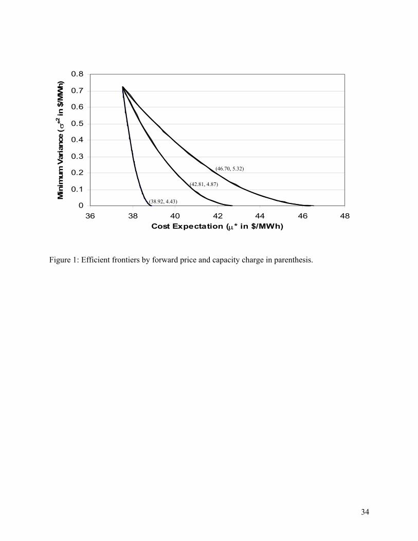
Figure 1 portrays the three efficient frontiers drawn under the three different assumed

forward prices and capacity charges of Table 4. The three frontiers share a common point at

which all electricity is procured through the spot market and regardless of the forward price and

capacity payment management places an upper limit of M = $37.52 on the per MWh expected

procurement cost that it is willing to incur. Total reliance on the spot market implies a maximum

risk, as reflected through the cost variance, of σ*2 = σ12 = 0.724, and a minimum expected cost of

µ* = µ1 = 37.52. By increasing the upper limit on the expected procurement cost management

can take advantage of electricity forwards and the tolling agreement to reduce the variance.

Indeed, the variance can be virtually eliminated through forward contracts. Regardless of the

forward price and the capacity payment, however, even when varying optimal mix among the

purchase alternatives in optimal fashion additional reductions in the variance become

20

increasingly costly. That is, the efficient frontiers are downward sloping and strictly convex. In

each case, however, the particular frontier shows both the minimum variance with which LDC

management must live at any given upper bound in the expected procurement cost, and

alternatively the minimum expected procurement cost that management must be prepared to

accept for a portfolio of options that entails a given level or risk, or variance.

The frontier closest to the vertical axis corresponds to the base-case values for the

forward price and the capacity payment. This first frontier is relatively steep because the

relatively low forward price of $38.92 and capacity payment of $4.43 permits a large reduction

in the portfolio’s cost variance through forward contracting and a tolling agreement, without

substantially raising the cost expectation, or the binding cap.

Immediately to the right of the base-case frontier is the one that is constructed with a

forward price and a capacity charge equal to 110% of the base-case values. This frontier is flatter

than the base-case frontier because the higher forward price and capacity charge implies that to

achieve the same variance reductions as those achieved with the base-case price and charge

requires larger expected procurement costs than in the base case. This is so, since variance

reductions can only be brought about by reduced reliance on the spot market.

The third and last frontier is constructed with a forward price and a capacity charge equal

to 120% of the base-case values. Although still convex, this frontier is the flattest among the

three frontiers. The flatness reflects the fact that reducing the portfolio’s cost variance by a given

amount has become more expensive than in the previous case.

Taken as a whole, the frontiers of Figure 1 affirm the intuition that at relatively low

forward prices and capacity charges, it is not very costly to reduce the risk of a procurement

portfolio. This affirmation would support management’s selection of a portfolio containing

21

relatively less spot purchase. But as forward prices and capacity charges rise, a binding budget

constraint will cause management to choose a portfolio with relatively more spot purchases.

6. Conclusions

Efficient frontiers have had steady employment as visually appealing and analytically

useful decision-making aids in a variety of multi-objective settings in which management has to

evaluate and choose among alternatives for which there are tradeoffs among those objectives.

Those settings extend well beyond mean-variance financial portfolio analysis [22] to hospitals

[43-44], mutual fund performance appraisal [45], managerial performance assessment [46],

regional development [47], marketing [48], and production [49].

Management of an LDC that must procure electricity to meet customer demand in real

time must also evaluate and choose among alternatives for which there are tradeoffs, in this case

between expected procurement cost and risk. In this novel setting, too, the efficient frontier is a

visually appealing and analytically useful decision-making aid. Developing the frontier,

however, is a rather complex proposition that involves determining the optimal blend of three

sources of electricity: the spot market, electricity forward contracts, and tolling agreements with

generators. Optimality in this context implies the blend that provides the minimum variance for a

given expected procurement cost. The frontier then traces out the tradeoffs that are available to

management between cost and risk. Those tradeoffs depend upon the price of electricity forwards

and the capacity payment in the tolling agreement.

Estimating the parameters that are required for assessing the expected costs and variances

is also a rather complex proposition. The complexities notwithstanding, this paper has shown

how to both estimate the parameters and develop the frontier, and how management can

determine its most preferred alternative on that frontier, given the tradeoffs that it is willing to

22

accept between cost and risk. Moreover, the paper has also shown that all of this is eminently

doable and immediately applicable. Thus, while one can hope that neither California nor any

other region will ever again confront an energy crisis of the sort that plagued the state and

punished end-users and LDCs alike from May 2000 to June 2001, it is our further hope that by

implementing the efficient-frontier approach management will not only be dealing with short-

term and unavoidable spot-price volatility in a prudent fashion, but will also be mitigating the

impact of any future crisis on both the company and its customers.

23

Acknowledgement

We thank two anonymous referees for their detailed comments and suggestions, which

helped us to greatly improve the paper’s exposition. Responsibility for any remaining errors rests

with us alone.

24

References

[1] Micheals RJ, Ellig J. Price spikes redux: a market emerged, remarkably rational. Public

Utilities Fortnightly 1999; 137(3): 40-47.

[2] Borenstein S. The trouble with electricity markets: understanding California’s

restructuring disaster. Journal of Economic Perspectives 2002; 16(1): 191-211.

[3] Borenstein S, Bushnell J, Knittel CR, Wolfram C. Trading inefficiencies in California

electricity markets. POWER Working Paper PWP-86. Berkeley, CA: University of

California Energy Institute, 2003.

[4] Krapels EN. Was gas to blame? Exploring the cause of California’s high prices. Public

Utilities Fortnightly 2001; 139(4): 28-36.

[5] Woo CK, Olson A, Horowitz I. Market efficiency, cross hedging and price forecasts:

California’s natural-gas markets. Working Paper. San Francisco, CA: Energy and

Environmental Economics, 2004.

[6] Faruqui A, Chao A-P, Niemeyer V, Platt J, Stahlkopf K. Analyzing California’s power

crisis. Energy Journal 2002; 22(4): 29-52.

[7] Woo CK. What went wrong in California’s electricity market? Energy – The

International Journal 2001; 26(8): 747-758.

[8] Blumenstein C, Friedman L, Green RJ. The history of electricity restructuring in

California. Journal of Industry and Competition and Trade 2002; 1(1/2): 9-38.

[9] Jurewitz JL. California electricity debacle: a guided tour. Electricity Journal 2002; 15(4):

10-29.

[10] Lee WW. US lessons for energy industry restructuring: based on natural gas and

California electricity incidences. Energy Policy 2004; 32(2): 237-259.

25

[11] Ellis DJ. A report on natural gas pricing and an evaluation of opportunities for price risk

management through various hedging options. West Virginia: Utilities Division, Public

Service Commission of West Virginia. 2001.

[12] EIA. Derivatives and risk management in the petroleum, natural gas and electricity

industries. Washington, D.C.: Energy Information Administration, U.S. Department of

Energy, 2002.

[13] Bessembinder H, Lemmon M. Equilibrium pricing and optimal hedging in electricity

forward markets. Journal of Finance 2002; 57(3): 1347-1382.

[14] Woo CK, Horowitz I, Horii B, Karimov R. The efficient frontier for spot and forward

purchases: an application to electricity. Journal of the Operational Research Society. In

press.

[15] Woo CK, Karimov R, Horowitz I. Managing electricity procurement cost and risk by a

local distribution company. Energy Policy 2004; 32(5): 635-645.

[16] Wolak FA. Diagnosing the California electricity crisis. Electricity Journal 2003; 16(7):

11-37.

[17] Woo CK, Lloyd D, Clayton W. Did a local distribution company procure prudently

during the California electricity crisis? Energy Policy. In press.

[18] Woo CK, Horowitz I, Hoang K. Cross hedging and value at risk: wholesale electricity

forward contracts. Advances in Investment Analysis and Portfolio Management 2001; 8:

283-301.

[19] Woo CK, Horowitz I, Hoang K. Cross hedging and forward-contract pricing of

electricity. Energy Economics 2001; 23(1): 1-15.

26

[20] Eydeland A, Wolyniec K. Energy and power risk management: new development in

modeling, pricing and hedging. New York: John Wiley, 2003.

[21] Deng SJ, Johnson R, Sogomonian A. Exotic electricity options and valuation of

electricity generation and transmission. Decision Support Systems 2001; 30(3): 383-392.

[22] Markowitz HM. Portfolio selection. New York: John Wiley, 1959.

[23] Takayama A. Mathematical economics. Hindale, IL: Dryden Press, 1974.

[24] Woo CK, Lloyd D, Borden M, Warrington R, Baskette C. A robust internet-based auction

to procure electricity forwards. Energy – The International Journal 2004; 29(1): 1-11.

[25] Serletis A, Herbert J. The message in North American energy prices. Energy Economics

1999; 21(5): 471-483.

[26] Doane MJ, Spulber DF. Open access and the evolution of the U.S. spot market for natural

gas. Journal of Law and Economics 1994; 37(2): 477-517.

[27] King M, Cuc M. Price convergence in North American natural gas spot markets. Energy

Journal 1996;17(2): 17-42.

[28] Serletis A. Is there an East-West split in North American natural gas markets? Energy

Journal 1997; 18(1): 47-62.

[29] Walls WD. An econometric analysis of the market for natural gas futures. Energy Journal

1995; 16(1): 71-83.

[30] Chen S-S, Lee C-f. Shresha K. Futures hedge ratios: a review. Quarterly Review of

Economics and Finance 2003; 43(3): 433-465.

[31] Kmenta J. Elements of econometrics. New York, NY: Macmillan, 1971.

[32] Fleten, S-E, Lemming J. Constructing forward price curves in electricity markets. Energy

Economics 2003; 25(5): 409-424.

27

[33] Keppo J, Lu H. Real options and a large producer: the case of electricity markets. Energy

Economics 2003; 25(5): 459-472.

[34] Spinler S, Huchzermeier A, Kleindorfer PR. The valuation of options on capacity.

Working Paper. Philadelphia, PA: The Wharton School, University of Pennsylvania,

2003.

[35] Efron B, Morris C. Limiting the risk of Bayes and empirical Bayes estimators – Part I:

the Bayes case. Journal of the American Statistical Association 1971; 66(336): 807-815.

[36] Efron B, Morris C. Limiting risk of Bayes and empirical Bayes estimators – Part II.

Journal of the American Statistical Association 1972; 67(337): 130-139.

[37] Efron, B. Large-scale simultaneous hypothesis testing: the choice of a null hypothesis.

Journal of the American Statistical Association 2004; 99(465): 96-104.

[38] Kamakura, WA, Wedel, M. An empirical Bayes procedure for improving individual-level

estimates and predictions from finite mixtures of multinomial logit models. Journal of

Business and Economic Statistics 2004; 22(1): 121-130.

[39] Maritz, JS, Lwin, T. Empirical Bayes methods (2nd edition). London: Chapman and Hall,

1989.

[40] Mood AM, Graybill FA, Boes DC. Introduction to the theory of statistics (3rd edition).

New York, NY: McGraw-Hill, 1974.

[41] Borenstein S, Bushnell JB, Wolak A. Measuring market inefficiencies in California’s

restructured wholesale electricity market. American Economic Review 2002; 92(5):

1376-1405.

[42] Pindyke RS, Rubinfeld DL. Econometric models and economic forecasts. New York,

NY: McGraw-Hill, 1991.

28

[43] Banker RD, Conrad RF, Straus RP. A comparative application of data envelopment

analysis and translog methods: an illustrative study of hospital production. Management

Science 1986; 32(1): 30-44.

[44] Kim SC, Horowitz I, Young KK, Buckley TA. Flexible bed allocation and performance

in the intensive care unit. Journal of Operations Management 2000; 18(4): 427-443.

[45] Morey MR, Morey RC. Mutual fund performance appraisals: a multi-horizon perspective

with endogenous benchmarking. Omega 1999; 27(2): 241-258.

[46] Thanassoulis E, Bussofiane A, Dyson RG. A comparison of data envelopment analysis

and ratio analysis as tools for performance assessment. Omega 1996; 24(3): 229244.

[47] Hibiki N, Sueyoshi R. DEA sensitivity analysis by changing a reference set: regional

contribution to Japanese industrial development. Omega 1999; 27(2): 139-153.

[48] Horsky D, Nelson P. Evaluation of sales force size and productivity through efficient

frontier benchmarking. Marketing Science 1996; 15(4): 301-326.

[49] De P, Ghosh JB, Wells CE. Heuristic estimation of the efficient frontier for a bi-criterion

scheduling problem. Decision Sciences 1992; 23(3): 596-609.

29

Table 1. Summary statistics, augmented Dickey-Fuller (ADF) statistics and pair-wise correlation coefficients for daily Mid-C spot electricity prices, daily per MWh variable cost of a tolling agreement with an 8,000 Btu/kWh heat rate, and daily Henry Hub spot natural-gas prices for the period of 07/02/01 – 09/02/03. Statistic Mid-C spot

electricity price

($/MWh)

Per MWh variable cost

($/MWh)

Henry Hub spot gas price ($/MMBtu)

Sumas spot gas price

($/MMBtu)

Mean 29.45 24.01 3.94 3.25 Standard deviation 13.60 10.63 1.52 1.33 ADF statistic -4.87* -3.13* -4.15* -2.47

1.0

0.80

0.59

0.67

0.80 1.0 0.84 0.93 0.59 0.84 1.0 0.94

Correlation coefficient: Mid-C price Per MWh variable cost Henry Hub gas price Sumas gas price 0.67 0.93 0.94 1.0

Note: “*” = “Significant at the 5% level”

30

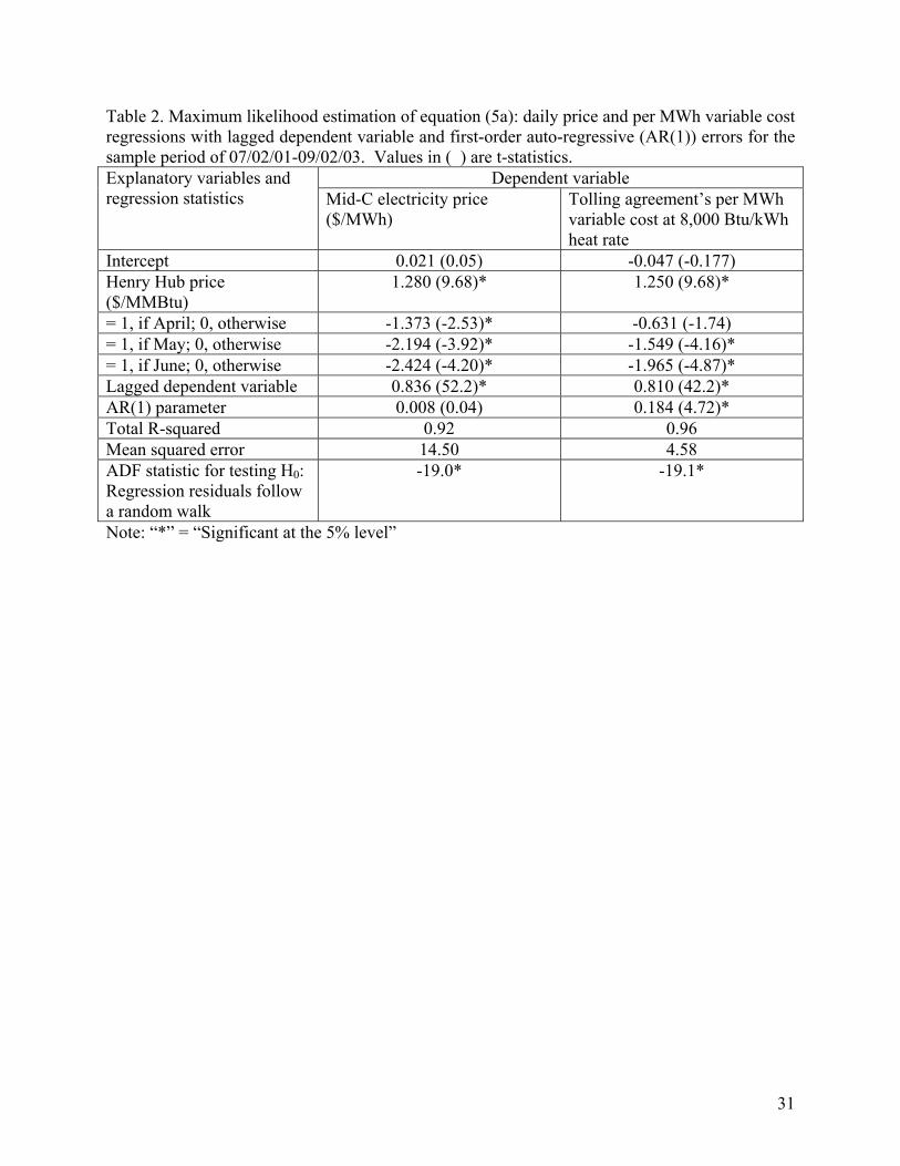
Table 2. Maximum likelihood estimation of equation (5a): daily price and per MWh variable cost regressions with lagged dependent variable and first-order auto-regressive (AR(1)) errors for the sample period of 07/02/01-09/02/03. Values in ( ) are t-statistics.

Dependent variable Explanatory variables and regression statistics Mid-C electricity price

($/MWh) Tolling agreement’s per MWh variable cost at 8,000 Btu/kWh heat rate

Intercept 0.021 (0.05) -0.047 (-0.177) Henry Hub price ($/MMBtu)

1.280 (9.68)* 1.250 (9.68)*

= 1, if April; 0, otherwise -1.373 (-2.53)* -0.631 (-1.74) = 1, if May; 0, otherwise -2.194 (-3.92)* -1.549 (-4.16)* = 1, if June; 0, otherwise -2.424 (-4.20)* -1.965 (-4.87)* Lagged dependent variable 0.836 (52.2)* 0.810 (42.2)* AR(1) parameter 0.008 (0.04) 0.184 (4.72)* Total R-squared 0.92 0.96 Mean squared error 14.50 4.58 ADF statistic for testing H0: Regression residuals follow a random walk

-19.0* -19.1*

Note: “*” = “Significant at the 5% level”

31

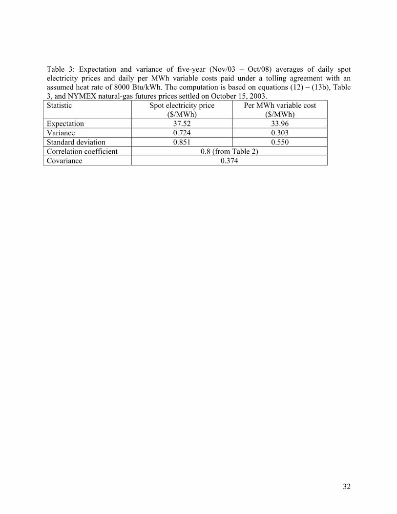
Table 3: Expectation and variance of five-year (Nov/03 – Oct/08) averages of daily spot electricity prices and daily per MWh variable costs paid under a tolling agreement with an assumed heat rate of 8000 Btu/kWh. The computation is based on equations (12) – (13b), Table 3, and NYMEX natural-gas futures prices settled on October 15, 2003. Statistic Spot electricity price

($/MWh) Per MWh variable cost

($/MWh) Expectation 37.52 33.96 Variance 0.724 0.303 Standard deviation 0.851 0.550 Correlation coefficient 0.8 (from Table 2) Covariance 0.374

32

Table 4: Assumed values for a 5-year forward contract’s price and a tolling agreement’s capacity payment. Assumption Forward price ($/MWh) Capacity payment ($/MWh) Base-case prices to effect profitability with 95% probability

38.92 4.43

110% of the base-case prices 42.81 4.87 120% of the base-case prices 46.70 5.32

33

0

0.1

0.2

0.3

0.4

0.5

0.6

0.7

0.8

36 38 40 42 44 46 48Cost Expectation (µ* in $/MWh)

Min

imum

Var

ianc

e ( σ

*2 in

$/M

Wh)

(46.70, 5.32)

(42.81, 4.87)

(38.92, 4.43)

Figure 1: Efficient frontiers by forward price and capacity charge in parenthesis.

34