Chewing the Cud on Using Multi-Commodity Hedge Ratios To Manage Dairy Farm Risk

by

John Newton, Cameron S. Thraen, and Marin Bozic

Suggested citation format:

Newton, J., C. S. Thraen, and M. Bozic. 2014. “Chewing the Cud on Using Multi-Commodity Hedge Ratios To Manage Dairy Farm Risk.” Proceedings of the NCCC-134 Conference on Applied Commodity Price Analysis, Forecasting, and Market Risk Management. St. Louis, MO. [http://www.farmdoc.illinois.edu/nccc134].

Chewing the Cud on Using Multi-Commodity Hedge

Ratios To Manage Dairy Farm Risk

John Newton †

Cameron S. Thraen ‡

and

Marin Bozic*

Paper presented at the NCCC-134 Conference on Applied Commodity Price Analysis, Forecasting, and Market Risk Management St. Louis, Missouri, April 21-

22, 2014.

Copyright 2014 by John Newton, Cameron S. Thraen, and Marin Bozic. All rights reserved. Readers may make verbatim copies of this document for non-commercial

purposes by any means, provided that this copyright notice appears on all such copies.

† Department of Agricultural and Consumer Economics, University of Illinois at Urbana-Champaign, Urbana 61801

‡ Department of Agricultural, Environmental & Development Economics, The Ohio State University, Columbus 43210

* Department of Applied Economics, University of Minnesota – Twin Cities, Saint Paul 55108

2

Chewing the Cud on Using Multi-Commodity Hedge Ratios To

Manage Dairy Farm Risk

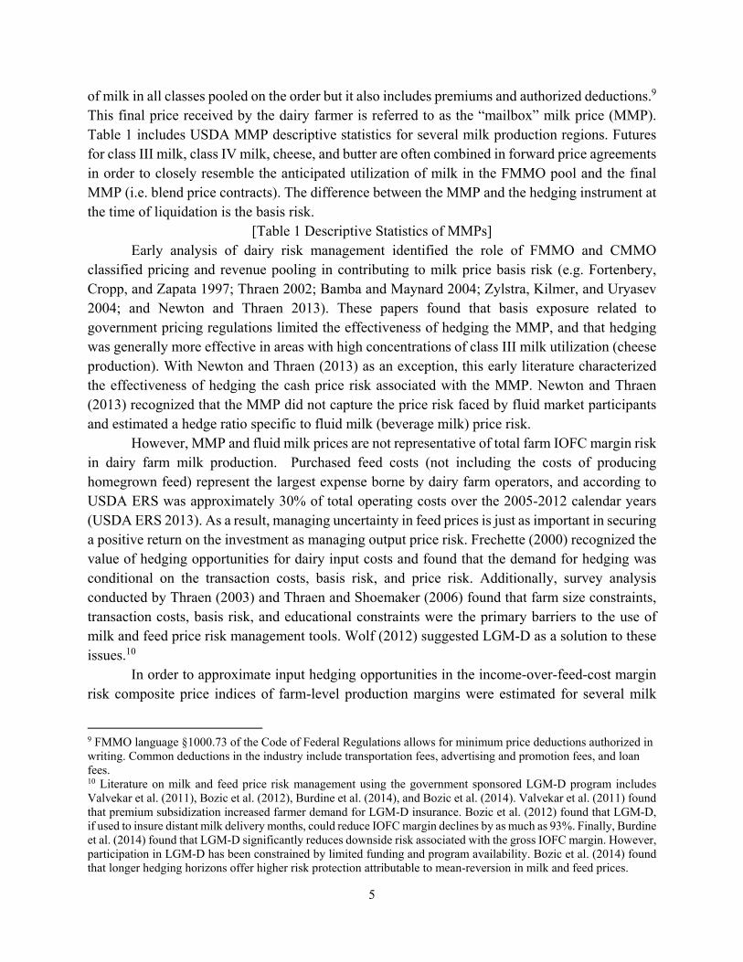
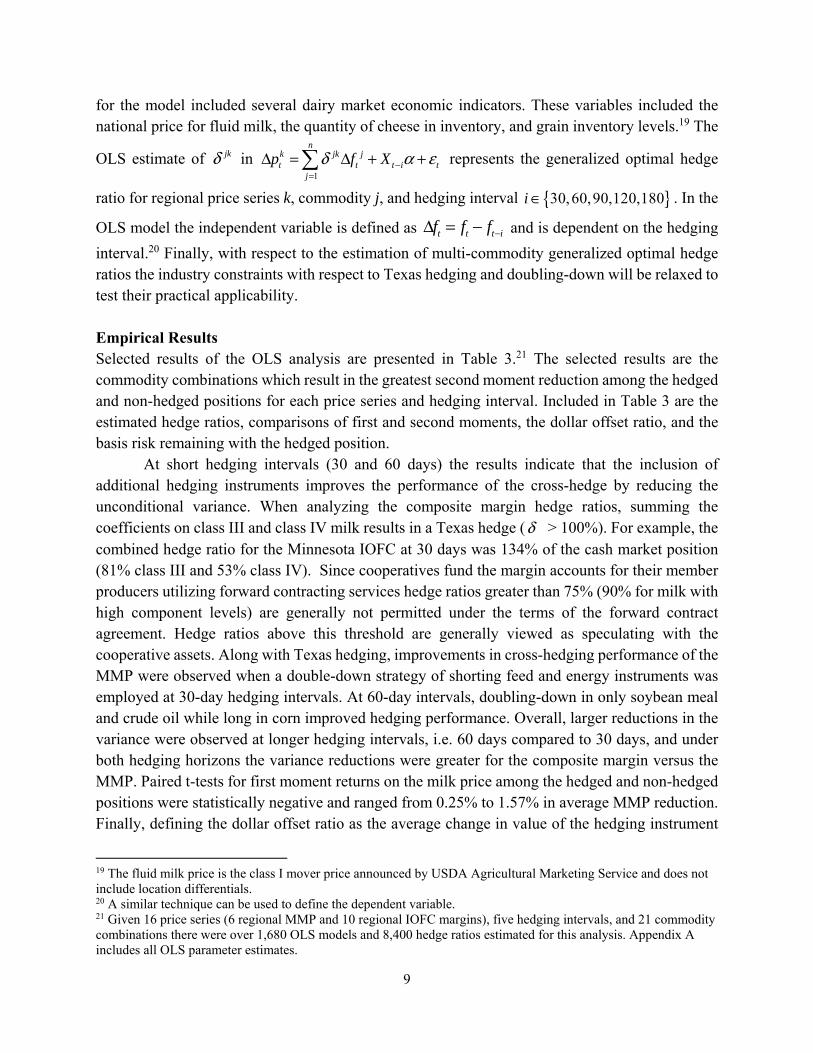
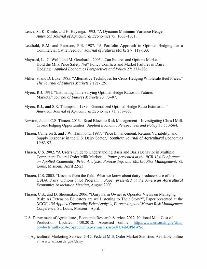
Abstract This study examines the risk management opportunities for regional mailbox milk prices and composite income-over-feed-cost margins using alternative milk and input cost risk management strategies. Multi-commodity hedge ratios are estimated using cash and futures market data over 2001 to 2013. Our analysis shows that at sufficient hedging horizons single- or multi-commodity hedge ratios may reduce up to 65% of the margin price risk, 39% of the milk price risk, and may outperform naïve pricing arrangements designed to replicate regulated milk pricing provisions. Cross-hedging using milk and feed futures is an imperfect hedge and remains exposed to basis risk due to the spatial value of feed and the regulatory burden of Federal and State milk pricing and pooling programs. Keywords: Dairy, Hedge Ratio, Multi-Commodity Hedge, Basis The gradual shift away from USDA public stockholding programs towards countercyclical payment and export assistance programs in the early 1990’s is believed to have partially contributed to the observed increases in milk price variability, Figure 1 (Thraen and Hammond 1987; Blayney and Normile 2004). Compounding price volatility concerns, low milk prices coupled with high feed costs have resulted in negative total farm profits for many U.S. dairy farm families (USDA ERS 2012). In light of these realities, dairy farm operators and managers have expressed a renewed interest in the use of a variety of farm risk management instruments to manage revenue and income-over-feed-cost (IOFC) margin risk. These instruments include futures and options contracts, forward contracts, financial swaps, and Livestock Gross Margin Insurance for Dairy (LGM-D).1

[Insert Figure 1 About Here] However, futures market contract design specifications, basis exposure on feed and milk,

and liquidity constraints in the dairy complex limit the dairy farm hedging opportunities of private risk markets and to some extent LGM-D (Newton and Thraen 2013). 2 To address these issues dairy farmer-owned cooperative associations, and where allowed, proprietary manufacturing plants have begun to offer a variety of risk management services to milk producers.3 These services

1 The 2014 Farm Bill creates a new risk management program in the form of a Margin Protection Program for Dairy producers. 2 CME Group milk futures contracts size is 200,000 pounds of milk and are cash settled against USDA announced class prices. CME Croup corn futures contract size is 5,000 bushels and are physically delivered upon expiration. CME group soybean meal contract size is 100 short tons and are physically delivered upon expiration. 3 The 2008 Farm Bill established the Dairy Forward Pricing Program and allows forward price contracts between milk processors (non-fluid) and dairy farmers (Newton and Thraen 2013). The Dairy Forward Pricing Program allows for the forward pricing of milk through September 2018. The Dairy Forward Pricing Program is not applicable for milk pooled on the California Milk Marketing Order.

3

involve the use of non-standardized forward milk price contracts and to a lesser extent forward pricing of feed ingredients and energy (e.g. corn silage, haylage, soybean meal, and fuel). The risk associated with the forward price agreement is generally aggregated by the cooperative or manufacturing plant and laid off in futures markets using the applicable derivative instruments.4 These forward pricing agreements serve three primary purposes: (i) the use of cooperative or plant financial resources eliminates the need for an individual dairy farmer to maintain a margin account; (ii) the forward prices may be customized to accommodate anticipated basis; and (iii) forward contract arrangements allow dairy farmers of all herd sizes an opportunity to reduce uncertainty and lock-in a return over their operating costs.

The purpose of this article is to examine the risk management potential of alternative milk and input cost risk management strategies. Emphasis will be placed on the flexibility of forward and futures contracts to accommodate spatial and temporal basis as well as hedging interval length. Empirical price relationships among Chicago Mercantile Exchange (CME) futures markets prices for milk, feed, and energy variables and their regional cash price counterparts will be used to determine how regional basis and the hedging interval may change the optimal hedging strategy when managing milk price or margin risk.5 This work builds on the work of Anderson and Danthine (1981), Leuthold and Peterson (1987), Myers and Thompson (1989), Fortenbery, Cropp, and Zapata (1997), Fortenbery, and Zapata (1997), Bamba and Maynard (2004), Maynard, Wolf, and Gearhardt (2005), and Newton and Thraen (2013) for the selection and combinations of milk, feed and energy assets to manage dairy farm risk.

We proceed with a brief discussion of how USDA Federal Milk Marketing Order (FMMO) and the California Milk Marketing Order (CMMO) pricing regulations contribute to milk price basis and then introduce state-level dairy production margins using USDA milk and feed price data. Next, using CME futures prices for milk, feed, and energy price variables we estimate generalized optimal hedge ratios (Myers and Thompson 1989) for various commodity combinations at several non-overlapping hedging horizons for each of the milk price and dairy production margins analyzed. The first and second moments of the hedged and non-hedged positions are compared to form conclusions on the effectiveness of the dairy farm risk management strategies. Finally, the ratio of price changes among the hedged and non-hedged price series are calculated to determine if the risk management strategies satisfy Financial Accounting Standards Board No. 133 (FASB 133) dollar offset ratio thresholds of 80% to 125% (Charnes, Koch and Berkman 2003). We conclude by demonstrating that highly customized forward contracts are an effective risk management strategy and have the potential to reduce more than 65% of the variation in the farm-level dairy production margin at sufficient hedging intervals. However, due to the basis exposure and inability to directly hedge, FASB 133 dollar offset ratio thresholds are seldom fulfilled.

4 For example eight 25 thousand pound milk forward contracts can be combined to form a short position in milk futures at the 200,000 pounds contract size. 5 The margin risk relies on the assumption that all feed is purchased monthly at prevailing cash prices.

4

Milk Price and Dairy Margin Risk Across the U.S., with California as a major exception, the USDA regulates milk and dairy

product prices using the FMMO.6 Marketing orders were established in Agricultural Marketing Agreement Act 1937 to help ensure that participating dairy farmers receive a minimum price for milk sold to milk processors and manufacturers (Blayney and Normile 2004). This is accomplished through the use of end-product price formulas, formal discriminatory pricing based on milk utilization, and revenue-sharing pools. The classified pricing system assigns monthly minimum milk prices based on the utilization of milk in each of four product classes: class I (beverage milk), class II (soft manufactured products), class III (cheese), and class IV (butter and milk powder). FMMO minimum milk prices for each class are calculated using pricing formulas that incorporate wholesale dairy product prices for cheddar cheese, butter, nonfat dry milk, and dry whey. The minimum price paid to producers pooling on a FMMO is the weighted average (i.e. “blend price”) value of all uses at the classified values and milk component levels (e.g. butterfat, protein, and other solids). Through the revenue pooling process all farmers delivering pooled milk share in the total revenue generated by all uses of milk regardless of how the milk of an individual dairy farmer is used.7

California has regulated its dairy industry under their own milk pricing plan and revenue pooling arrangement and has remained autonomous from the rest of the U.S. and the FMMO program. The California program differs from the FMMO program in that it operates a quota program and it has five end-use classes of milk. The classes of milk are as follows: class 1 (beverage milk), class 2 (cultured products), class 3 (frozen products), class 4a (butter and milk powder), and class 4b (cheese and whey). Revenue pooling in the CMMO depends on the amount of quota a producer owns. The quota provides a separate source of revenue for dairy producers in the state. Producers in the state are paid on the basis of their allocated quota milk and their non-quota milk at prices which reflect the utilization of milk in the California market. To summarize, both the CMMO and the FMMO classified pricing and pooling systems regulate prices paid by dairy processors and as price discrimination and income support schemes are designed to increase dairy farmer producer surplus. The CME does not list blend price contracts which reflect FMMO or CMMO weighted average milk prices; instead, it offers futures and options contracts on manufacturing milk (FMMO class III and class IV) and storable dairy products.8 With these contracts it is difficult to directly manage the blend price risk because the CME includes only two milk futures contracts (FMMO class III/IV prices) and the final price received by the dairy farmer represents not only the value

6 There are presently ten FMMO marketing areas in the U.S. Information on FMMOs can be found online at: www.ams.usda.gov/dairy 7 The FMMO blend price is the minimum price and dairy farmers often negotiate premiums over and above the FMMO minimum. Premiums are often paid on the basis of milk quality and delivery volume incentives. 8 The CME also offers spot, futures and options contracts on cheddar cheese (weighted average of block and barrels), butter, non-fat dry milk, whey, and international skim milk powder. The CME does not have a futures or options contract for fluid beverage milk (Newton and Thraen 2013). The CME does not have a futures contract for CMMO classes of milk; however, CMMO milk price formulas incorporate CME spot prices for block cheddar cheese, butter, and nonfat dry milk directly.

5

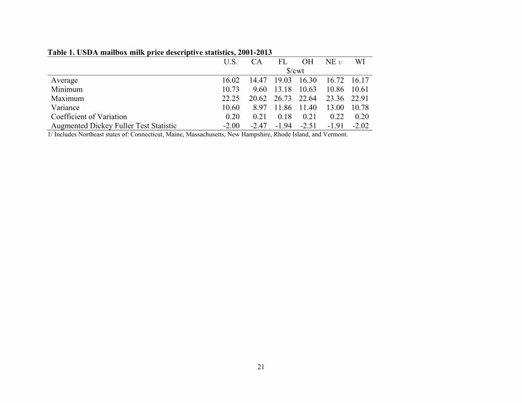
of milk in all classes pooled on the order but it also includes premiums and authorized deductions.9 This final price received by the dairy farmer is referred to as the “mailbox” milk price (MMP). Table 1 includes USDA MMP descriptive statistics for several milk production regions. Futures for class III milk, class IV milk, cheese, and butter are often combined in forward price agreements in order to closely resemble the anticipated utilization of milk in the FMMO pool and the final MMP (i.e. blend price contracts). The difference between the MMP and the hedging instrument at the time of liquidation is the basis risk.

[Table 1 Descriptive Statistics of MMPs] Early analysis of dairy risk management identified the role of FMMO and CMMO

classified pricing and revenue pooling in contributing to milk price basis risk (e.g. Fortenbery, Cropp, and Zapata 1997; Thraen 2002; Bamba and Maynard 2004; Zylstra, Kilmer, and Uryasev 2004; and Newton and Thraen 2013). These papers found that basis exposure related to government pricing regulations limited the effectiveness of hedging the MMP, and that hedging was generally more effective in areas with high concentrations of class III milk utilization (cheese production). With Newton and Thraen (2013) as an exception, this early literature characterized the effectiveness of hedging the cash price risk associated with the MMP. Newton and Thraen (2013) recognized that the MMP did not capture the price risk faced by fluid market participants and estimated a hedge ratio specific to fluid milk (beverage milk) price risk.

However, MMP and fluid milk prices are not representative of total farm IOFC margin risk in dairy farm milk production. Purchased feed costs (not including the costs of producing homegrown feed) represent the largest expense borne by dairy farm operators, and according to USDA ERS was approximately 30% of total operating costs over the 2005-2012 calendar years (USDA ERS 2013). As a result, managing uncertainty in feed prices is just as important in securing a positive return on the investment as managing output price risk. Frechette (2000) recognized the value of hedging opportunities for dairy input costs and found that the demand for hedging was conditional on the transaction costs, basis risk, and price risk. Additionally, survey analysis conducted by Thraen (2003) and Thraen and Shoemaker (2006) found that farm size constraints, transaction costs, basis risk, and educational constraints were the primary barriers to the use of milk and feed price risk management tools. Wolf (2012) suggested LGM-D as a solution to these issues.10

In order to approximate input hedging opportunities in the income-over-feed-cost margin risk composite price indices of farm-level production margins were estimated for several milk

9 FMMO language §1000.73 of the Code of Federal Regulations allows for minimum price deductions authorized in writing. Common deductions in the industry include transportation fees, advertising and promotion fees, and loan fees. 10 Literature on milk and feed price risk management using the government sponsored LGM-D program includes Valvekar et al. (2011), Bozic et al. (2012), Burdine et al. (2014), and Bozic et al. (2014). Valvekar et al. (2011) found that premium subsidization increased farmer demand for LGM-D insurance. Bozic et al. (2012) found that LGM-D, if used to insure distant milk delivery months, could reduce IOFC margin declines by as much as 93%. Finally, Burdine et al. (2014) found that LGM-D significantly reduces downside risk associated with the gross IOFC margin. However, participation in LGM-D has been constrained by limited funding and program availability. Bozic et al. (2014) found that longer hedging horizons offer higher risk protection attributable to mean-reversion in milk and feed prices.

6

producing states. The composite margins were standardized based on the dairy production margin formula in the 2014 Farm Bill Margin Protection Program for dairy producers.11 Using data from USDA on regional milk and feed prices, dairy production margins were calculated such that the margin is equal to ( ), , , ,1.0728 0.00735 0.0137k k k k

t AMP t C t SBM t H tM p p p p= − × + × + × for k=U.S.,

Illinois, Iowa, Michigan, Minnesota, Ohio, Pennsylvania, Texas, and Wisconsin regions and 1,...,156t = months (2001-2013).12 The variables in the production margin include: AMPp is the

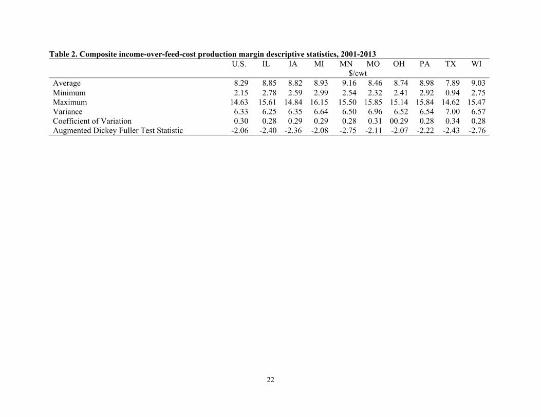
USDA Agricultural Statistics Service (NASS) announced all-milk price per hundredweight for region k, Cp is the USDA NASS announced corn price per bushel for region k, SBMp is the USDA Agricultural Marketing Service announced central Illinois high protein soybean meal price per ton, and Hp is the USDA NASS announced alfalfa hay price per ton for region k.13 Table 2 includes descriptive statistics for the composite dairy production margins.

[Table 2 Descriptive Statistics of Margins] As demonstrated in table 2 there is a noticeable variation in the composite dairy production

margin averages, and one-way ANOVA tests indicate that the sample means were significantly different. However, comparing the coefficients of variation composite margins have similar levels of dispersion. Differences in margins are due to milk and feed price basis. For example, due to higher FMMO utilization in lower manufacturing classes and higher purchased feed costs in Texas the average production margin was $0.39 per hundredweight below the U.S. average. Meanwhile Minnesota, partially due to lower feed costs, had an average production margin that was $0.74 per hundredweight above the national average. Differences in farm and animal productivity due to climate conditions, land resources, and availability of conventional purchased feed alternatives help to facilitate large-scale intensive dairy operations with associated economies of scale and different cost structures. As a result, comparing margins across regions is not directly indicative of relative farm viability and profitability. In this analysis comparisons serve only to differentiate the cross-hedging strategy and measure performance.

In order to manage the margin risk a combination of manufacturing milk futures and futures contracts for the underlying feed components may be employed. For example, seven milk futures contracts (1.4 million pounds of milk), three corn contracts, and one soybean meal contract would result in an implied margin that contains 1.071 corn bushels and 0.00714 tons of soybean meal per hundredweight of milk – closely resembling the 2014 Farm Bill feed ration coefficients.14 Given that 70% of U.S. dairy farms have fewer than 200 milking cows, and produce less than four million 11 The margin Protection Program for dairy producers is a margin insurance program designed to pay an indemnity to a participating farm when the difference between the national average all-milk price and the formula-derived estimate of total herd feed costs falls below a farmer-selected margin trigger. 12 Due to data availability constraints the soybean meal price is not adjusted regionally. The time period analyzed includes January 2001 to December 2013. 13 The IOFC margin formula was derived through collaboration with animal scientists and includes the costs of feeding milking cows, hospital cows, dry cows, and replacement heifers. The fixed coefficients in the feed ration calculation are based on a generic cost of feeding dairy cows (National Milk Producers Federation 2010). 14 15,000 bushels divided by 14,000 hundredweight of milk is 1.071 corn bushels per hundredweight of milk. 100 short tons divided by 14,000 hundredweight of milk is 0.00714 tons of soybean meal per hundredweight of milk.

7

pounds of milk per year, such a technique, if employed monthly, would only be feasible for largest dairy operations (i.e. approximately 770 cows).15 Additionally, due to the lack of alfalfa hay futures, the effect of forward pricing on the USDA published prices, and milk and feed price basis, such a combination of instruments may not adequately replicate the risks at the farm level – ultimately leaving a large portion of cash positions unhedged.16 Finally, semi-naïve hedge ratios on the milk and feed components may be sub-optimal if the desired result is a reduction in the price or margin variability.17 Due to these constraints, forward contracts, when allowable, are often employed to more directly manage milk price and margin risk.

Forward contracts provide dairy farmers an opportunity to partially customize a cross-hedging strategy to manage farm-level risks in milk production. Forward contract specifications include but are not limited to: monthly, quarterly, semi-annual, or annual price contracts; blend price contracts; and cross-hedging using milk and feed instruments. The length of the forward contract in the specifications is straightforward, but blend price contracts and cross-hedging with feed instruments is more complex. A blend price contract involves constructing a forward price of milk that resembles the USDA FMMO weighted average utilization (or blend price) of milk in the marketing area. Cross-hedging with milk and feed instruments involves establishing a forward price equal to the price of milk less the cost of purchased feeds and (potentially) energy. In each case the forward price is based on prevailing futures market prices for the underlying commodities.

Under the terms of these forward price agreements farmers are not permitted to double-down by going against their natural position (e.g. going long in milk) or to hedge greater than 100% of their cash market exposure (i.e. Texas hedge). Leuthold and Peterson (1987) found that portfolio risk increases at a much faster rate when employing a Texas hedge. While seemingly exotic relative to a futures market contract these forward contracts are often very rigid in design structure such that they are not fully customized to the needs of the individual dairy farmers and do not wholly account for farm-level milk and feed price basis. Additionally, the forward contracts employed are often static such that the contract parameters do not change as the hedging interval increases.18 To determine how much customization is required to manage farm-level milk prices and margins an empirical analysis of the relationship among futures and regional cash prices will

15 Seven milk futures contracts would represent 1.4 million pounds of monthly production and is equivalent to a 770 cow dairy at 21,822 U.S. annual production pounds per cow. Due to CME futures contract specifications recreating similar margin coefficient weights using CME futures may not be possible for individual dairymen below this production threshold. 16 USDA published prices for milk, corn, and alfalfa hay may include prices negotiated under a forward price agreement. The forward prices are not included until the expiration date of the forward price agreement. For example, USDA reported corn prices for March may include prices for corn contracted in December post-harvest (same marketing year). 17 Other objective functions could be considered such as minimizing downside risk (semi-variance), time-varying optimal hedge ratio (Myers 1991) or a dynamic minimum variance hedge ratio (Lence, Kimle, and Hayenga 1993). With respect to the time-varying and dynamic minimum variance approaches only negligible differences in hedging effectiveness relative to the constant generalized optimal hedge ratio were observed. 18 Information on proprietary forward contracting services offered by farmer-owned cooperatives and manufacturing plants were obtained from confidential industry sources.

8

be used to determine how basis and the hedging interval may change the optimal hedging strategy for single- or multi-commodity hedge ratios.

Multi-Commodity Generalized Optimal Hedge Ratios In order to identify the proportion of futures market positions that should be used to cover the spot market position multi-commodity hedge ratios may be used. Multi-commodity hedge ratios differ from a single commodity hedge ratio because they account for futures price pair interactions among the commodities. Chen, Lee, and Shrestha (2003) provide a review of different theoretical approaches to optimal futures hedge ratios and concluded that no single optimal hedge ratio technique is superior in hedging performance.

For estimation of the optimal multi-commodity hedge ratios we review Anderson and Danthine (1981), Miller and Luke (1985), Myers and Thompson (1989), Fackler and McNew (1993), and Grant (1995). Based on this literature the hedge ratios for this analysis are Myers and Thompson (1989) generalized optimal (multi-commodity) hedge ratios. Based on the Myers and Thompson framework, dairy farmer profit in period t is denoted:

( ) ( )1 1 1 11

nj j j

t t t t t t tj

p q c q h f fπ − − − −=

= − − − where π is profit, p is the cash price, 1tq − is milk

production, ( )c ⋅ is a cost function, jf is the futures price for commodity j, and jh is the sales of

futures contracts (purchase if negative) for 1,...,j n= commodities. The farmer then chooses q and h to maximize the mean and minimize the variance of profit, conditional on available information

1tX − . The first order conditions for this problem yields the hedging rule:

( )( )1 11 11 1 1 1

111 10

j jt t t t tf E f X qλ− −− − − −

−= Σ − + Σ Σh where 1t−h is a 1n × vector of futures contract

positions 1j

th − for 1,...,j n= , λ is the farmer’s risk aversion, 11Σ is an n n× partition of the variance/covariance matrix and 10Σ is a 1n × partition of the variance/covariance matrix (Anderson and Danthine 1981). The first term on the RHS is the pure speculative position and the second term on the RHS is the pure hedging position. With the assumption of an unbiased futures market

( )1 1j j

t t tE f X f− −= , and mean-variance efficiency, it follows that the optimal hedge ratio is given

by: 111 11 10

1

jj t

tt

hqδ ∗ −−

−−

= = Σ Σ and allows for price pair interactions among the milk, feed, and energy

variables to influence the hedging position. Based on an augmented Dickey-Fuller test for a unit root, the null hypothesis that the milk

and margin prices were non-stationary and possessed a unit root could not be rejected, Tables 1 and 2. Due to the results of the stationarity tests first differences for the dependent variable estimations were imposed to improve estimation efficiency. The multi-commodity hedge ratios were obtained using an augmented reduced form model of the cash milk price returns and cash production margin returns with the change in the underlying futures assets over the life of the hedge (hedging interval) as the augmenting variable. The relevant conditioning information, 1tX −

9

for the model included several dairy market economic indicators. These variables included the national price for fluid milk, the quantity of cheese in inventory, and grain inventory levels.19 The

OLS estimate of jkδ in 1

nk jk jt t t i t

jp f Xδ α ε−

=

Δ = Δ + + represents the generalized optimal hedge

ratio for regional price series k, commodity j, and hedging interval { }30,60,90,120,180i ∈ . In the

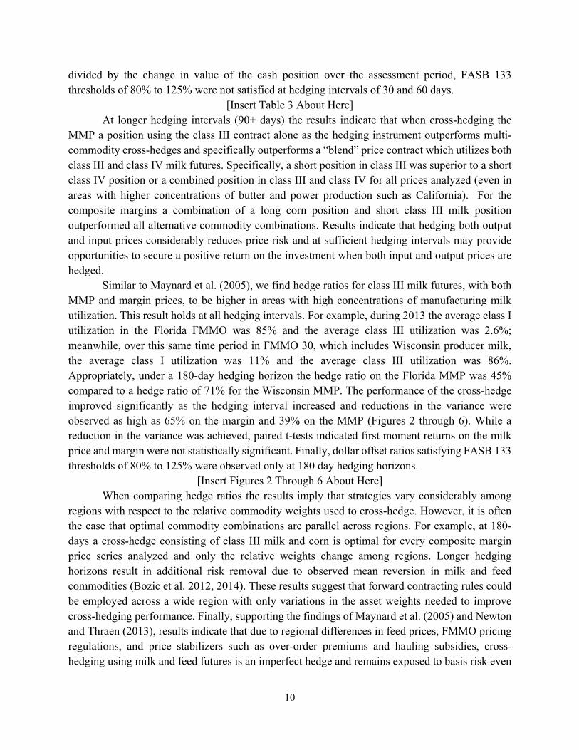
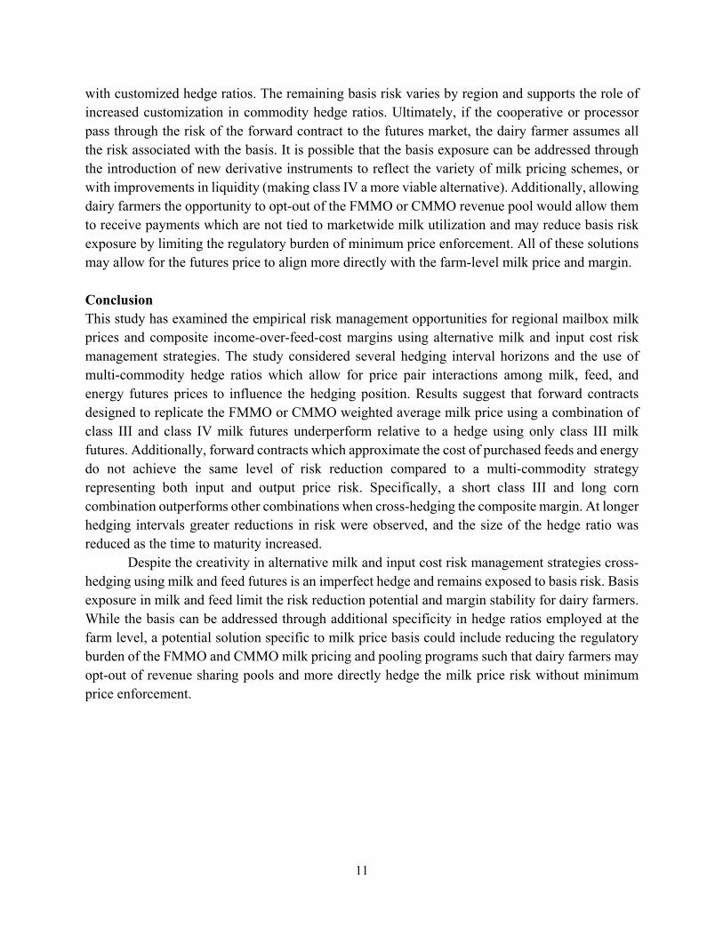
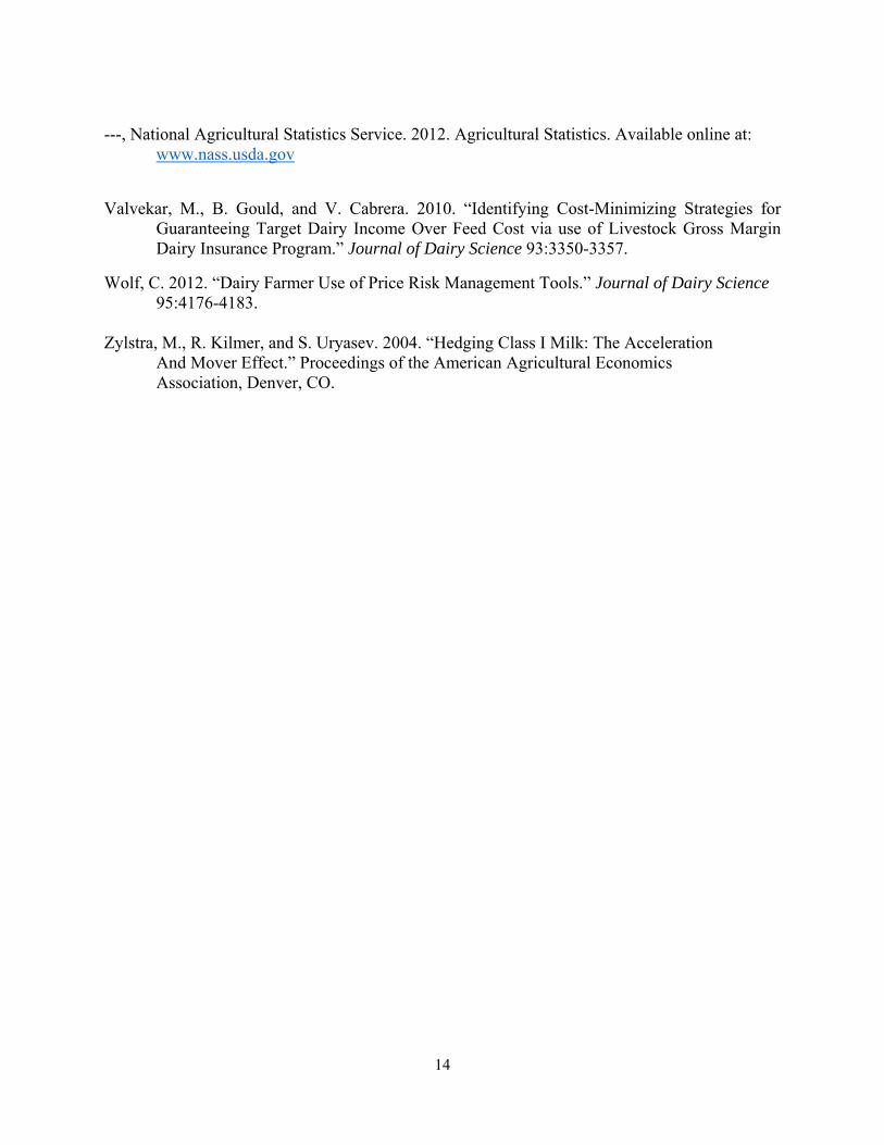
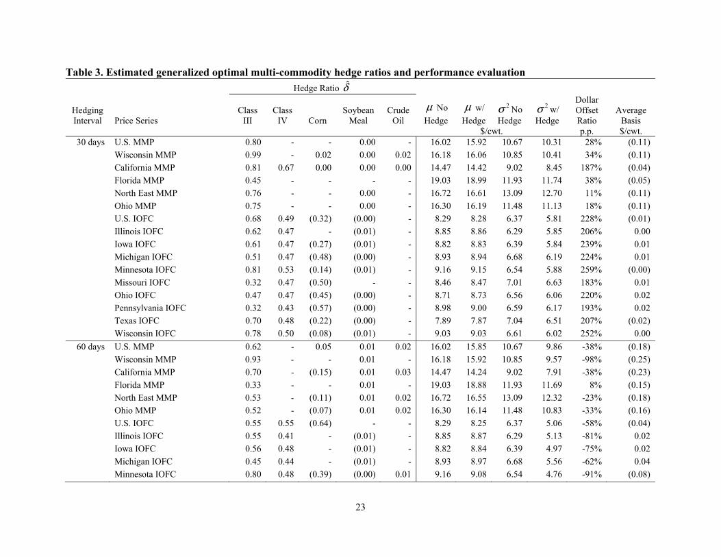
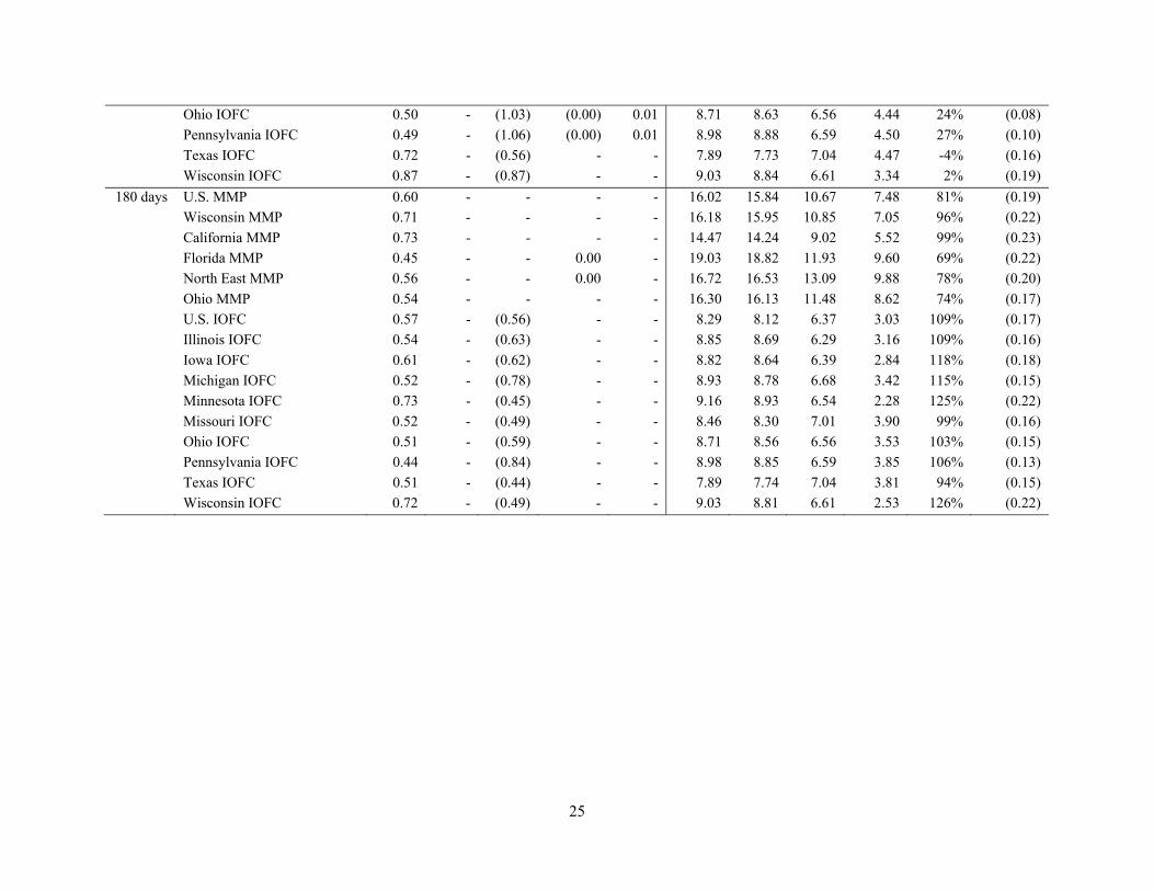
OLS model the independent variable is defined as t t t if f f −Δ = − and is dependent on the hedging interval.20 Finally, with respect to the estimation of multi-commodity generalized optimal hedge ratios the industry constraints with respect to Texas hedging and doubling-down will be relaxed to test their practical applicability. Empirical Results Selected results of the OLS analysis are presented in Table 3.21 The selected results are the commodity combinations which result in the greatest second moment reduction among the hedged and non-hedged positions for each price series and hedging interval. Included in Table 3 are the estimated hedge ratios, comparisons of first and second moments, the dollar offset ratio, and the basis risk remaining with the hedged position. At short hedging intervals (30 and 60 days) the results indicate that the inclusion of additional hedging instruments improves the performance of the cross-hedge by reducing the unconditional variance. When analyzing the composite margin hedge ratios, summing the coefficients on class III and class IV milk results in a Texas hedge (δ > 100%). For example, the combined hedge ratio for the Minnesota IOFC at 30 days was 134% of the cash market position (81% class III and 53% class IV). Since cooperatives fund the margin accounts for their member producers utilizing forward contracting services hedge ratios greater than 75% (90% for milk with high component levels) are generally not permitted under the terms of the forward contract agreement. Hedge ratios above this threshold are generally viewed as speculating with the cooperative assets. Along with Texas hedging, improvements in cross-hedging performance of the MMP were observed when a double-down strategy of shorting feed and energy instruments was employed at 30-day hedging intervals. At 60-day intervals, doubling-down in only soybean meal and crude oil while long in corn improved hedging performance. Overall, larger reductions in the variance were observed at longer hedging intervals, i.e. 60 days compared to 30 days, and under both hedging horizons the variance reductions were greater for the composite margin versus the MMP. Paired t-tests for first moment returns on the milk price among the hedged and non-hedged positions were statistically negative and ranged from 0.25% to 1.57% in average MMP reduction. Finally, defining the dollar offset ratio as the average change in value of the hedging instrument

19 The fluid milk price is the class I mover price announced by USDA Agricultural Marketing Service and does not include location differentials. 20 A similar technique can be used to define the dependent variable. 21 Given 16 price series (6 regional MMP and 10 regional IOFC margins), five hedging intervals, and 21 commodity combinations there were over 1,680 OLS models and 8,400 hedge ratios estimated for this analysis. Appendix A includes all OLS parameter estimates.

10

divided by the change in value of the cash position over the assessment period, FASB 133 thresholds of 80% to 125% were not satisfied at hedging intervals of 30 and 60 days.

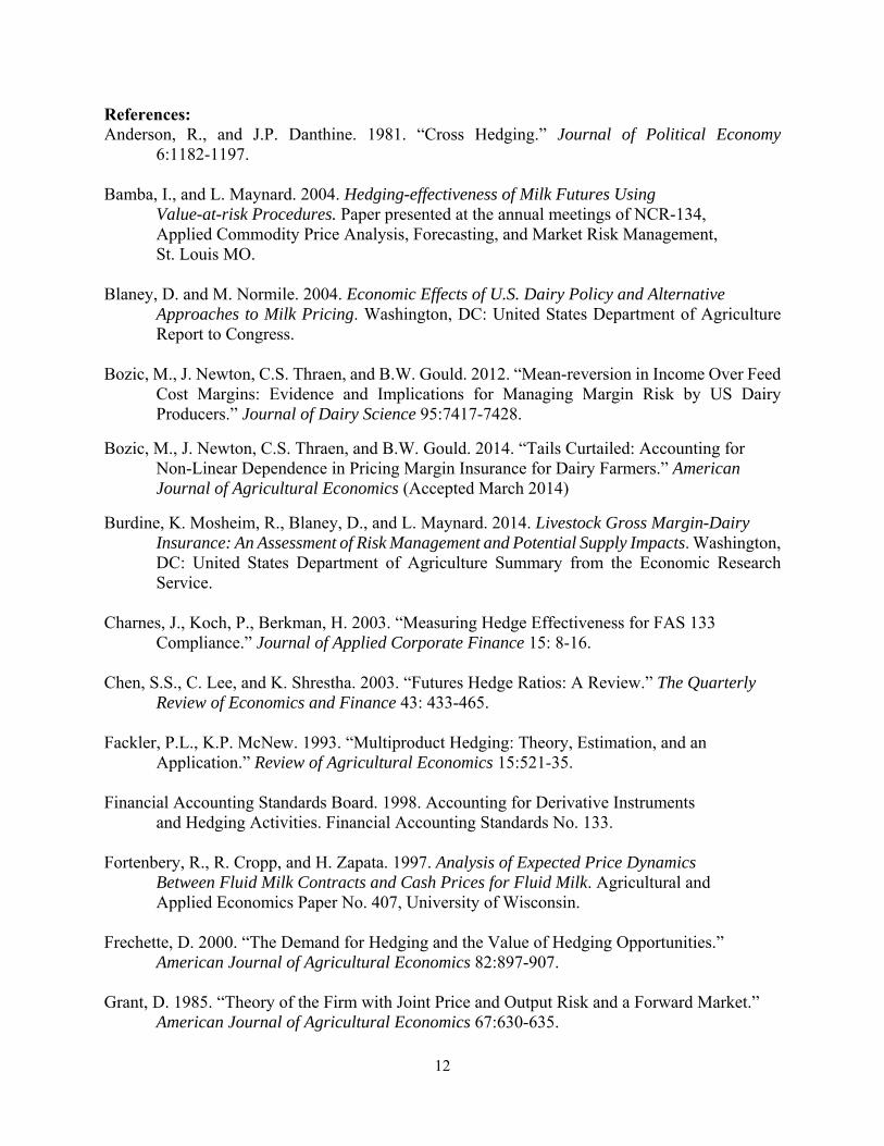
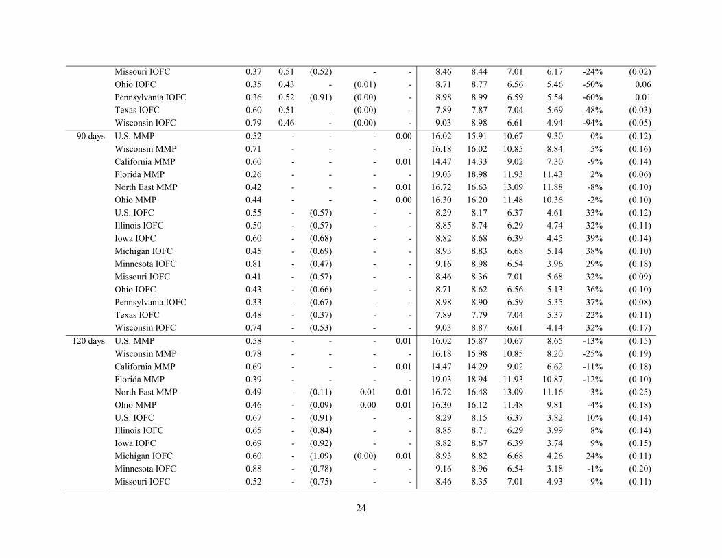
[Insert Table 3 About Here] At longer hedging intervals (90+ days) the results indicate that when cross-hedging the MMP a position using the class III contract alone as the hedging instrument outperforms multi-commodity cross-hedges and specifically outperforms a “blend” price contract which utilizes both class III and class IV milk futures. Specifically, a short position in class III was superior to a short class IV position or a combined position in class III and class IV for all prices analyzed (even in areas with higher concentrations of butter and power production such as California). For the composite margins a combination of a long corn position and short class III milk position outperformed all alternative commodity combinations. Results indicate that hedging both output and input prices considerably reduces price risk and at sufficient hedging intervals may provide opportunities to secure a positive return on the investment when both input and output prices are hedged.

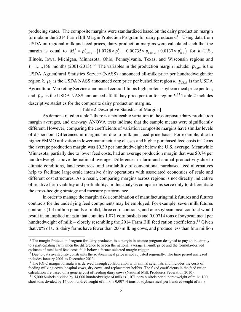
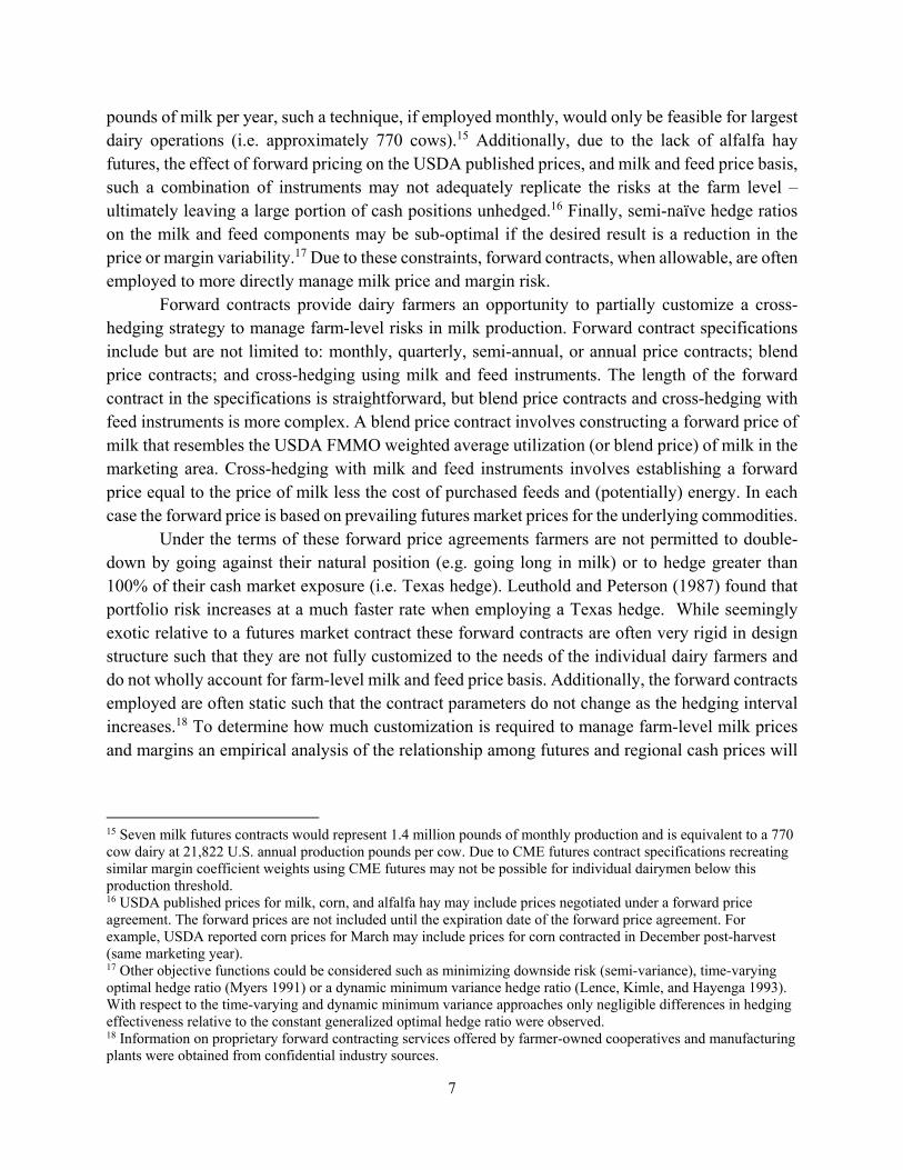
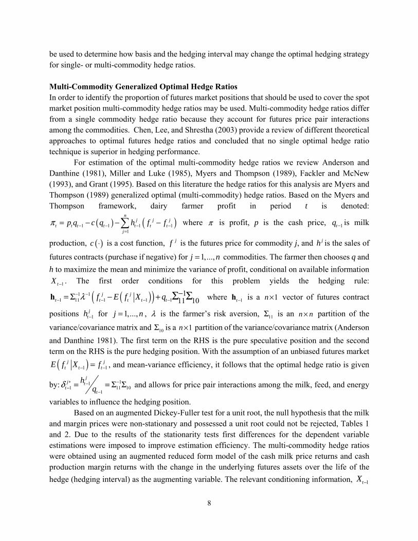
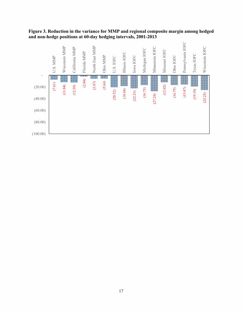
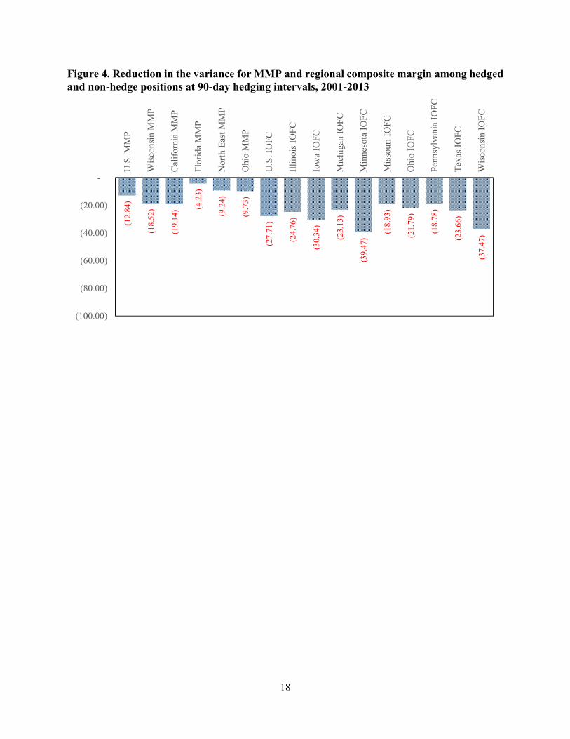
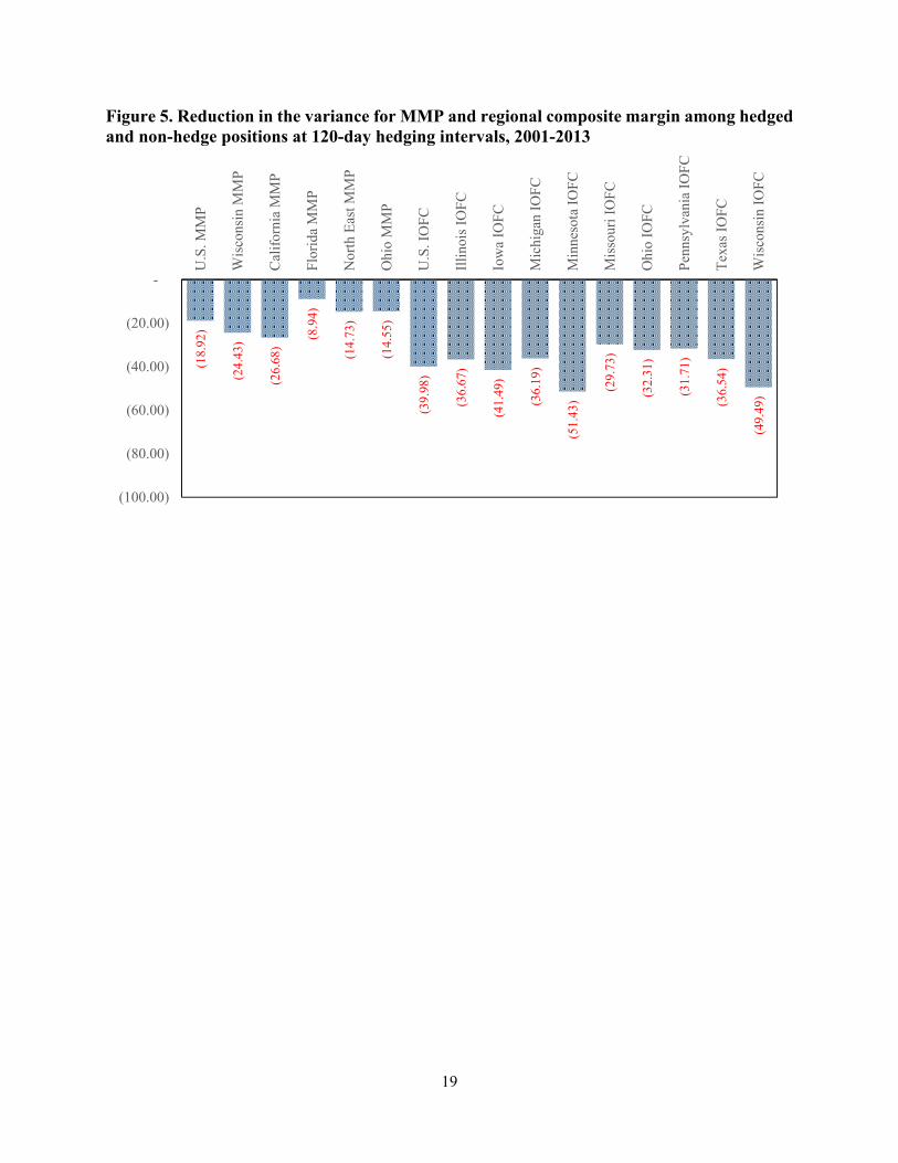
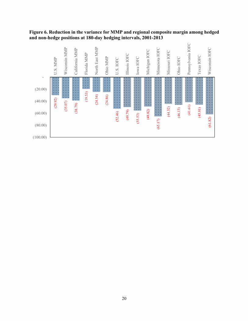
Similar to Maynard et al. (2005), we find hedge ratios for class III milk futures, with both MMP and margin prices, to be higher in areas with high concentrations of manufacturing milk utilization. This result holds at all hedging intervals. For example, during 2013 the average class I utilization in the Florida FMMO was 85% and the average class III utilization was 2.6%; meanwhile, over this same time period in FMMO 30, which includes Wisconsin producer milk, the average class I utilization was 11% and the average class III utilization was 86%. Appropriately, under a 180-day hedging horizon the hedge ratio on the Florida MMP was 45% compared to a hedge ratio of 71% for the Wisconsin MMP. The performance of the cross-hedge improved significantly as the hedging interval increased and reductions in the variance were observed as high as 65% on the margin and 39% on the MMP (Figures 2 through 6). While a reduction in the variance was achieved, paired t-tests indicated first moment returns on the milk price and margin were not statistically significant. Finally, dollar offset ratios satisfying FASB 133 thresholds of 80% to 125% were observed only at 180 day hedging horizons.

[Insert Figures 2 Through 6 About Here] When comparing hedge ratios the results imply that strategies vary considerably among

regions with respect to the relative commodity weights used to cross-hedge. However, it is often the case that optimal commodity combinations are parallel across regions. For example, at 180-days a cross-hedge consisting of class III milk and corn is optimal for every composite margin price series analyzed and only the relative weights change among regions. Longer hedging horizons result in additional risk removal due to observed mean reversion in milk and feed commodities (Bozic et al. 2012, 2014). These results suggest that forward contracting rules could be employed across a wide region with only variations in the asset weights needed to improve cross-hedging performance. Finally, supporting the findings of Maynard et al. (2005) and Newton and Thraen (2013), results indicate that due to regional differences in feed prices, FMMO pricing regulations, and price stabilizers such as over-order premiums and hauling subsidies, cross-hedging using milk and feed futures is an imperfect hedge and remains exposed to basis risk even

11

with customized hedge ratios. The remaining basis risk varies by region and supports the role of increased customization in commodity hedge ratios. Ultimately, if the cooperative or processor pass through the risk of the forward contract to the futures market, the dairy farmer assumes all the risk associated with the basis. It is possible that the basis exposure can be addressed through the introduction of new derivative instruments to reflect the variety of milk pricing schemes, or with improvements in liquidity (making class IV a more viable alternative). Additionally, allowing dairy farmers the opportunity to opt-out of the FMMO or CMMO revenue pool would allow them to receive payments which are not tied to marketwide milk utilization and may reduce basis risk exposure by limiting the regulatory burden of minimum price enforcement. All of these solutions may allow for the futures price to align more directly with the farm-level milk price and margin. Conclusion This study has examined the empirical risk management opportunities for regional mailbox milk prices and composite income-over-feed-cost margins using alternative milk and input cost risk management strategies. The study considered several hedging interval horizons and the use of multi-commodity hedge ratios which allow for price pair interactions among milk, feed, and energy futures prices to influence the hedging position. Results suggest that forward contracts designed to replicate the FMMO or CMMO weighted average milk price using a combination of class III and class IV milk futures underperform relative to a hedge using only class III milk futures. Additionally, forward contracts which approximate the cost of purchased feeds and energy do not achieve the same level of risk reduction compared to a multi-commodity strategy representing both input and output price risk. Specifically, a short class III and long corn combination outperforms other combinations when cross-hedging the composite margin. At longer hedging intervals greater reductions in risk were observed, and the size of the hedge ratio was reduced as the time to maturity increased.

Despite the creativity in alternative milk and input cost risk management strategies cross-hedging using milk and feed futures is an imperfect hedge and remains exposed to basis risk. Basis exposure in milk and feed limit the risk reduction potential and margin stability for dairy farmers. While the basis can be addressed through additional specificity in hedge ratios employed at the farm level, a potential solution specific to milk price basis could include reducing the regulatory burden of the FMMO and CMMO milk pricing and pooling programs such that dairy farmers may opt-out of revenue sharing pools and more directly hedge the milk price risk without minimum price enforcement.

12

References: Anderson, R., and J.P. Danthine. 1981. “Cross Hedging.” Journal of Political Economy 6:1182-1197. Bamba, I., and L. Maynard. 2004. Hedging-effectiveness of Milk Futures Using

Value-at-risk Procedures. Paper presented at the annual meetings of NCR-134, Applied Commodity Price Analysis, Forecasting, and Market Risk Management, St. Louis MO.

Blaney, D. and M. Normile. 2004. Economic Effects of U.S. Dairy Policy and Alternative

Approaches to Milk Pricing. Washington, DC: United States Department of Agriculture Report to Congress.

Bozic, M., J. Newton, C.S. Thraen, and B.W. Gould. 2012. “Mean-reversion in Income Over Feed

Cost Margins: Evidence and Implications for Managing Margin Risk by US Dairy Producers.” Journal of Dairy Science 95:7417-7428.

Bozic, M., J. Newton, C.S. Thraen, and B.W. Gould. 2014. “Tails Curtailed: Accounting for Non-Linear Dependence in Pricing Margin Insurance for Dairy Farmers.” American Journal of Agricultural Economics (Accepted March 2014)

Burdine, K. Mosheim, R., Blaney, D., and L. Maynard. 2014. Livestock Gross Margin-Dairy Insurance: An Assessment of Risk Management and Potential Supply Impacts. Washington, DC: United States Department of Agriculture Summary from the Economic Research Service.

Charnes, J., Koch, P., Berkman, H. 2003. “Measuring Hedge Effectiveness for FAS 133

Compliance.” Journal of Applied Corporate Finance 15: 8-16. Chen, S.S., C. Lee, and K. Shrestha. 2003. “Futures Hedge Ratios: A Review.” The Quarterly

Review of Economics and Finance 43: 433-465. Fackler, P.L., K.P. McNew. 1993. “Multiproduct Hedging: Theory, Estimation, and an

Application.” Review of Agricultural Economics 15:521-35. Financial Accounting Standards Board. 1998. Accounting for Derivative Instruments

and Hedging Activities. Financial Accounting Standards No. 133. Fortenbery, R., R. Cropp, and H. Zapata. 1997. Analysis of Expected Price Dynamics

Between Fluid Milk Contracts and Cash Prices for Fluid Milk. Agricultural and Applied Economics Paper No. 407, University of Wisconsin.

Frechette, D. 2000. “The Demand for Hedging and the Value of Hedging Opportunities.”

American Journal of Agricultural Economics 82:897-907.

Grant, D. 1985. “Theory of the Firm with Joint Price and Output Risk and a Forward Market.” American Journal of Agricultural Economics 67:630-635.

13

Lence, S., K. Kimle, and H. Hayenga. 1993. “A Dynamic Minimum Variance Hedge.”

American Journal of Agricultural Economics 75: 1063–1071.

Leuthold, R.M. and Peterson, P.E. 1987. “A Portfolio Approach to Optimal Hedging for a Commercial Cattle Feedlot.” Journal of Futures Markets 7: 119-133. Maynard, L., C. Wolf, and M. Gearhardt. 2005. “Can Futures and Options Markets

Hold the Milk Price Safety Net? Policy Conflicts and Market Failures in Dairy Hedging.” Applied Economics Perspectives and Policy 27: 273–286.

Miller, S. and D. Luke. 1985. “Alternative Techniques for Cross-Hedging Wholesale Beef Prices.”

The Journal of Futures Markets 2:121-129. Myers, R.J. 1991. “Estimating Time-varying Optimal Hedge Ratios on Futures

Markets.” Journal of Futures Markets 20: 73–87. Myers, R.J., and S.R. Thompson. 1989. “Generalized Optimal Hedge Ratio Estimation.”

American Journal of Agricultural Economics 71: 858–868.

Newton, J., and C.S. Thraen. 2013. “Road Block to Risk Management – Investigating Class I Milk Cross-Hedging Opportunities” Applied Economic Perspectives and Policy 35:550-564.

Thraen, Cameron S. and J.W. Hammond. 1987. “Price Enhancement, Returns Variability, and Supply Response in the U.S. Dairy Sector,” Southern Journal of Agricultural Economics 19:83-92.

Thraen, C.S. 2002. “A User’s Guide to Understanding Basis and Basis Behavior in Multiple

Component Federal Order Milk Markets.”, Paper presented at the NCR-134 Conference on Applied Commodity Price Analysis, Forecasting, and Market Risk Management, St. Louis, Missouri, April 22-23.

Thraen, C.S. 2003. “Lessons from the field: What we know about dairy producers use of the

USDA Dairy Options Pilot Program.”, Paper presented at the American Agricultural Economics Association Meeting, August 2003.

Thraen, C.S., and D. Shoemaker. 2006. “Dairy Farm Owner & Operator Views on Managing

Risk: As Extension Educators are we Listening to Their Story?”, Paper presented at the NCCC-134 Applied Commodity Price Analysis, Forecasting and Market Risk Management Conference, St. Louis, Missouri, April.

U.S. Department of Agriculture., Economic Research Service. 2012. National Milk Cost of

Production Updated 1/30.2012. Accessed online: http://www.ers.usda.gov/data-products/milk-cost-of-production-estimates.aspx#.U4ibGPldWSo

---, Agricultural Marketing Service. 2012. Federal Milk Order Market Statistics. Available online

at: www.ams.usda.gov/dairy

14

---, National Agricultural Statistics Service. 2012. Agricultural Statistics. Available online at: www.nass.usda.gov

Valvekar, M., B. Gould, and V. Cabrera. 2010. “Identifying Cost-Minimizing Strategies for Guaranteeing Target Dairy Income Over Feed Cost via use of Livestock Gross Margin Dairy Insurance Program.” Journal of Dairy Science 93:3350-3357.

Wolf, C. 2012. “Dairy Farmer Use of Price Risk Management Tools.” Journal of Dairy Science 95:4176-4183.

Zylstra, M., R. Kilmer, and S. Uryasev. 2004. “Hedging Class I Milk: The Acceleration

And Mover Effect.” Proceedings of the American Agricultural Economics Association, Denver, CO.

15

Figure 1. USDA U.S. All-Milk Price, 1960-2013

0

5

10

15

20

2519

60

1970

1980

1990

2000

2010

$/cw

t

16

Figure 2. Reduction in the variance for MMP and regional composite margin among hedged and non-hedge positions at 30-day hedging intervals, 2001-2013

(3.3

7)

(4.1

0)

(6.4

1)

(1.6

0)

(2.9

6)

(3.0

0)

(8.7

7)

(7.0

5)

(8.6

9)

(7.2

9)

(10.

08)

(5.4

2)

(7.5

7)

(6.3

5)

(7.5

2)

(9.0

7)

(100.00)

(80.00)

(60.00)

(40.00)

(20.00)

-

U.S

. MM

P

Wisc

onsin

MM

P

Calif

orni

a M

MP

Flor

ida

MM

P

Nor

th E

ast M

MP

Ohi

o M

MP

U.S

. IO

FC

Illin

ois I

OFC

Iow

a IO

FC

Mic

higa

n IO

FC

Min

neso

ta IO

FC

Miss

ouri

IOFC

Ohi

o IO

FC

Penn

sylv

ania

IOFC

Texa

s IO

FC

Wisc

onsin

IOFC

17

Figure 3. Reduction in the variance for MMP and regional composite margin among hedged and non-hedge positions at 60-day hedging intervals, 2001-2013

(7.6

1)

(11.

84)

(12.

39) (2.0

4)

(5.8

7)

(5.6

4)

(20.

52)

(18.

44)

(22.

21)

(16.

75)

(27.

24) (1

2.02

)

(16.

75)

(15.

87)

(19.

19)

(25.

25)

(100.00)

(80.00)

(60.00)

(40.00)

(20.00)

-

U.S

. MM

P

Wisc

onsin

MM

P

Calif

orni

a M

MP

Flor

ida

MM

P

Nor

th E

ast M

MP

Ohi

o M

MP

U.S

. IO

FC

Illin

ois I

OFC

Iow

a IO

FC

Mic

higa

n IO

FC

Min

neso

ta IO

FC

Miss

ouri

IOFC

Ohi

o IO

FC

Penn

sylv

ania

IOFC

Texa

s IO

FC

Wisc

onsin

IOFC

18

Figure 4. Reduction in the variance for MMP and regional composite margin among hedged and non-hedge positions at 90-day hedging intervals, 2001-2013

(12.

84)

(18.

52)

(19.

14) (4

.23)

(9.2

4)

(9.7

3)

(27.

71)

(24.

76)

(30.

34)

(23.

13)

(39.

47)

(18.

93)

(21.

79)

(18.

78)

(23.

66)

(37.

47)

(100.00)

(80.00)

(60.00)

(40.00)

(20.00)

-

U.S

. MM

P

Wisc

onsin

MM

P

Calif

orni

a M

MP

Flor

ida

MM

P

Nor

th E

ast M

MP

Ohi

o M

MP

U.S

. IO

FC

Illin

ois I

OFC

Iow

a IO

FC

Mic

higa

n IO

FC

Min

neso

ta IO

FC

Miss

ouri

IOFC

Ohi

o IO

FC

Penn

sylv

ania

IOFC

Texa

s IO

FC

Wisc

onsin

IOFC

19

Figure 5. Reduction in the variance for MMP and regional composite margin among hedged and non-hedge positions at 120-day hedging intervals, 2001-2013

(18.

92)

(24.

43)

(26.

68)

(8.9

4)

(14.

73)

(14.

55)

(39.

98)

(36.

67)

(41.

49)

(36.

19)

(51.

43)

(29.

73)

(32.

31)

(31.

71)

(36.

54)

(49.

49)

(100.00)

(80.00)

(60.00)

(40.00)

(20.00)

-

U.S

. MM

P

Wisc

onsin

MM

P

Calif

orni

a M

MP

Flor

ida

MM

P

Nor

th E

ast M

MP

Ohi

o M

MP

U.S

. IO

FC

Illin

ois I

OFC

Iow

a IO

FC

Mic

higa

n IO

FC

Min

neso

ta IO

FC

Miss

ouri

IOFC

Ohi

o IO

FC

Penn

sylv

ania

IOFC

Texa

s IO

FC

Wisc

onsin

IOFC

20

Figure 6. Reduction in the variance for MMP and regional composite margin among hedged and non-hedge positions at 180-day hedging intervals, 2001-2013

(29.

92)

(35.

07)

(38.

79) (1

9.53

)

(24.

54)

(24.

86)

(52.

46)

(49.

79)

(55.

53)

(48.

82)

(65.

17)

(44.

32)

(46.

13)

(41.

61)

(45.

81)

(61.

82)

(100.00)

(80.00)

(60.00)

(40.00)

(20.00)

-

U.S

. MM

P

Wisc

onsin

MM

P

Calif

orni

a M

MP

Flor

ida

MM

P

Nor

th E

ast M

MP

Ohi

o M

MP

U.S

. IO

FC

Illin

ois I

OFC

Iow

a IO

FC

Mic

higa

n IO

FC

Min

neso

ta IO

FC

Miss

ouri

IOFC

Ohi

o IO

FC

Penn

sylv

ania

IOFC

Texa

s IO

FC

Wisc

onsin

IOFC

21

Table 1. USDA mailbox milk price descriptive statistics, 2001-2013 U.S. CA FL OH NE 1/ WI $/cwt Average 16.02 14.47 19.03 16.30 16.72 16.17Minimum 10.73 9.60 13.18 10.63 10.86 10.61Maximum 22.25 20.62 26.73 22.64 23.36 22.91Variance 10.60 8.97 11.86 11.40 13.00 10.78Coefficient of Variation 0.20 0.21 0.18 0.21 0.22 0.20Augmented Dickey Fuller Test Statistic -2.00 -2.47 -1.94 -2.51 -1.91 -2.02

1/ Includes Northeast states of: Connecticut, Maine, Massachusetts, New Hampshire, Rhode Island, and Vermont.

22

Table 2. Composite income-over-feed-cost production margin descriptive statistics, 2001-2013 U.S. IL IA MI MN MO OH PA TX WI $/cwt Average 8.29 8.85 8.82 8.93 9.16 8.46 8.74 8.98 7.89 9.03Minimum 2.15 2.78 2.59 2.99 2.54 2.32 2.41 2.92 0.94 2.75Maximum 14.63 15.61 14.84 16.15 15.50 15.85 15.14 15.84 14.62 15.47Variance 6.33 6.25 6.35 6.64 6.50 6.96 6.52 6.54 7.00 6.57Coefficient of Variation 0.30 0.28 0.29 0.29 0.28 0.31 00.29 0.28 0.34 0.28Augmented Dickey Fuller Test Statistic -2.06 -2.40 -2.36 -2.08 -2.75 -2.11 -2.07 -2.22 -2.43 -2.76

23

Table 3. Estimated generalized optimal multi-commodity hedge ratios and performance evaluation Hedge Ratio δ̂

Hedging Interval Price Series

Class III

Class IV Corn

Soybean Meal

Crude Oil

μ No Hedge

μ w/ Hedge

2σ No Hedge

2σ w/ Hedge

Dollar Offset Ratio

Average Basis

$/cwt. p.p. $/cwt. 30 days U.S. MMP 0.80 - - 0.00 - 16.02 15.92 10.67 10.31 28% (0.11)

Wisconsin MMP 0.99 - 0.02 0.00 0.02 16.18 16.06 10.85 10.41 34% (0.11) California MMP 0.81 0.67 0.00 0.00 0.00 14.47 14.42 9.02 8.45 187% (0.04) Florida MMP 0.45 - - - - 19.03 18.99 11.93 11.74 38% (0.05) North East MMP 0.76 - - 0.00 - 16.72 16.61 13.09 12.70 11% (0.11) Ohio MMP 0.75 - - 0.00 - 16.30 16.19 11.48 11.13 18% (0.11) U.S. IOFC 0.68 0.49 (0.32) (0.00) - 8.29 8.28 6.37 5.81 228% (0.01) Illinois IOFC 0.62 0.47 - (0.01) - 8.85 8.86 6.29 5.85 206% 0.00 Iowa IOFC 0.61 0.47 (0.27) (0.01) - 8.82 8.83 6.39 5.84 239% 0.01 Michigan IOFC 0.51 0.47 (0.48) (0.00) - 8.93 8.94 6.68 6.19 224% 0.01 Minnesota IOFC 0.81 0.53 (0.14) (0.01) - 9.16 9.15 6.54 5.88 259% (0.00) Missouri IOFC 0.32 0.47 (0.50) - - 8.46 8.47 7.01 6.63 183% 0.01 Ohio IOFC 0.47 0.47 (0.45) (0.00) - 8.71 8.73 6.56 6.06 220% 0.02 Pennsylvania IOFC 0.32 0.43 (0.57) (0.00) - 8.98 9.00 6.59 6.17 193% 0.02 Texas IOFC 0.70 0.48 (0.22) (0.00) - 7.89 7.87 7.04 6.51 207% (0.02) Wisconsin IOFC 0.78 0.50 (0.08) (0.01) - 9.03 9.03 6.61 6.02 252% 0.00

60 days U.S. MMP 0.62 - 0.05 0.01 0.02 16.02 15.85 10.67 9.86 -38% (0.18) Wisconsin MMP 0.93 - - 0.01 - 16.18 15.92 10.85 9.57 -98% (0.25) California MMP 0.70 - (0.15) 0.01 0.03 14.47 14.24 9.02 7.91 -38% (0.23) Florida MMP 0.33 - - 0.01 - 19.03 18.88 11.93 11.69 8% (0.15) North East MMP 0.53 - (0.11) 0.01 0.02 16.72 16.55 13.09 12.32 -23% (0.18) Ohio MMP 0.52 - (0.07) 0.01 0.02 16.30 16.14 11.48 10.83 -33% (0.16) U.S. IOFC 0.55 0.55 (0.64) - - 8.29 8.25 6.37 5.06 -58% (0.04) Illinois IOFC 0.55 0.41 - (0.01) - 8.85 8.87 6.29 5.13 -81% 0.02 Iowa IOFC 0.56 0.48 - (0.01) - 8.82 8.84 6.39 4.97 -75% 0.02 Michigan IOFC 0.45 0.44 - (0.01) - 8.93 8.97 6.68 5.56 -62% 0.04 Minnesota IOFC 0.80 0.48 (0.39) (0.00) 0.01 9.16 9.08 6.54 4.76 -91% (0.08)

24

Missouri IOFC 0.37 0.51 (0.52) - - 8.46 8.44 7.01 6.17 -24% (0.02) Ohio IOFC 0.35 0.43 - (0.01) - 8.71 8.77 6.56 5.46 -50% 0.06 Pennsylvania IOFC 0.36 0.52 (0.91) (0.00) - 8.98 8.99 6.59 5.54 -60% 0.01 Texas IOFC 0.60 0.51 - (0.00) - 7.89 7.87 7.04 5.69 -48% (0.03) Wisconsin IOFC 0.79 0.46 - (0.00) - 9.03 8.98 6.61 4.94 -94% (0.05)

90 days U.S. MMP 0.52 - - - 0.00 16.02 15.91 10.67 9.30 0% (0.12) Wisconsin MMP 0.71 - - - - 16.18 16.02 10.85 8.84 5% (0.16) California MMP 0.60 - - - 0.01 14.47 14.33 9.02 7.30 -9% (0.14) Florida MMP 0.26 - - - - 19.03 18.98 11.93 11.43 2% (0.06) North East MMP 0.42 - - - 0.01 16.72 16.63 13.09 11.88 -8% (0.10) Ohio MMP 0.44 - - - 0.00 16.30 16.20 11.48 10.36 -2% (0.10) U.S. IOFC 0.55 - (0.57) - - 8.29 8.17 6.37 4.61 33% (0.12) Illinois IOFC 0.50 - (0.57) - - 8.85 8.74 6.29 4.74 32% (0.11) Iowa IOFC 0.60 - (0.68) - - 8.82 8.68 6.39 4.45 39% (0.14) Michigan IOFC 0.45 - (0.69) - - 8.93 8.83 6.68 5.14 38% (0.10) Minnesota IOFC 0.81 - (0.47) - - 9.16 8.98 6.54 3.96 29% (0.18) Missouri IOFC 0.41 - (0.57) - - 8.46 8.36 7.01 5.68 32% (0.09) Ohio IOFC 0.43 - (0.66) - - 8.71 8.62 6.56 5.13 36% (0.10) Pennsylvania IOFC 0.33 - (0.67) - - 8.98 8.90 6.59 5.35 37% (0.08) Texas IOFC 0.48 - (0.37) - - 7.89 7.79 7.04 5.37 22% (0.11) Wisconsin IOFC 0.74 - (0.53) - - 9.03 8.87 6.61 4.14 32% (0.17) 120 days U.S. MMP 0.58 - - - 0.01 16.02 15.87 10.67 8.65 -13% (0.15) Wisconsin MMP 0.78 - - - - 16.18 15.98 10.85 8.20 -25% (0.19) California MMP 0.69 - - - 0.01 14.47 14.29 9.02 6.62 -11% (0.18) Florida MMP 0.39 - - - - 19.03 18.94 11.93 10.87 -12% (0.10) North East MMP 0.49 - (0.11) 0.01 0.01 16.72 16.48 13.09 11.16 -3% (0.25) Ohio MMP 0.46 - (0.09) 0.00 0.01 16.30 16.12 11.48 9.81 -4% (0.18) U.S. IOFC 0.67 - (0.91) - - 8.29 8.15 6.37 3.82 10% (0.14) Illinois IOFC 0.65 - (0.84) - - 8.85 8.71 6.29 3.99 8% (0.14) Iowa IOFC 0.69 - (0.92) - - 8.82 8.67 6.39 3.74 9% (0.15) Michigan IOFC 0.60 - (1.09) (0.00) 0.01 8.93 8.82 6.68 4.26 24% (0.11) Minnesota IOFC 0.88 - (0.78) - - 9.16 8.96 6.54 3.18 -1% (0.20) Missouri IOFC 0.52 - (0.75) - - 8.46 8.35 7.01 4.93 9% (0.11)

25

Ohio IOFC 0.50 - (1.03) (0.00) 0.01 8.71 8.63 6.56 4.44 24% (0.08) Pennsylvania IOFC 0.49 - (1.06) (0.00) 0.01 8.98 8.88 6.59 4.50 27% (0.10) Texas IOFC 0.72 - (0.56) - - 7.89 7.73 7.04 4.47 -4% (0.16) Wisconsin IOFC 0.87 - (0.87) - - 9.03 8.84 6.61 3.34 2% (0.19) 180 days U.S. MMP 0.60 - - - - 16.02 15.84 10.67 7.48 81% (0.19) Wisconsin MMP 0.71 - - - - 16.18 15.95 10.85 7.05 96% (0.22) California MMP 0.73 - - - - 14.47 14.24 9.02 5.52 99% (0.23) Florida MMP 0.45 - - 0.00 - 19.03 18.82 11.93 9.60 69% (0.22) North East MMP 0.56 - - 0.00 - 16.72 16.53 13.09 9.88 78% (0.20) Ohio MMP 0.54 - - - - 16.30 16.13 11.48 8.62 74% (0.17) U.S. IOFC 0.57 - (0.56) - - 8.29 8.12 6.37 3.03 109% (0.17) Illinois IOFC 0.54 - (0.63) - - 8.85 8.69 6.29 3.16 109% (0.16) Iowa IOFC 0.61 - (0.62) - - 8.82 8.64 6.39 2.84 118% (0.18) Michigan IOFC 0.52 - (0.78) - - 8.93 8.78 6.68 3.42 115% (0.15) Minnesota IOFC 0.73 - (0.45) - - 9.16 8.93 6.54 2.28 125% (0.22) Missouri IOFC 0.52 - (0.49) - - 8.46 8.30 7.01 3.90 99% (0.16) Ohio IOFC 0.51 - (0.59) - - 8.71 8.56 6.56 3.53 103% (0.15) Pennsylvania IOFC 0.44 - (0.84) - - 8.98 8.85 6.59 3.85 106% (0.13) Texas IOFC 0.51 - (0.44) - - 7.89 7.74 7.04 3.81 94% (0.15) Wisconsin IOFC 0.72 - (0.49) - - 9.03 8.81 6.61 2.53 126% (0.22)