Cheng, W. and Morrow, J. (2018) Firm productivity differences from factor

markets. The Journal of Industrial Economics, 66(1), pp. 126-

171. (doi:10.1111/joie.12165)

There may be differences between this version and the published version.

You are advised to consult the publisher’s version if you wish to cite from

it.

Cheng, W. and Morrow, J. (2018) Firm productivity differences from factor

markets. The Journal of Industrial Economics, 66(1), pp. 126-

171. (doi:10.1111/joie.12165)

This article may be used for non-commercial purposes in accordance with

Wiley Terms and Conditions for Self-Archiving.

http://eprints.gla.ac.uk/161408/

Deposited on: 25 June 2018

FIRM PRODUCTIVITY DIFFERENCES FROM FACTOR

MARKETS∗

Wenya Cheng†

John Morrow‡

Abstract

We model firm adaptation to local factor markets in which firms care about both

the price and availability of inputs. The model is estimated by combining firm and

population census data, and quantifies the role of factor markets in input use, pro-

ductivity and welfare. Considering China’s diverse factor markets, we find within

industry interquartile labor costs vary by 30-80%, leading to 3-12% interquartile

differences in TFP. In general equilibrium, homogenization of labor markets would

increase real income by 1.33%. Favorably endowed regions attract more economic

activity, providing new insights into within-country comparative advantage and

specialization.

I. INTRODUCTION

Although firms may face radically different production conditions, this

∗We thank Maria Bas, Andy Bernard, Loren Brandt, Sabine D’Costa, Fabrice Defever, Swati Dhingra,Ben Faber, Garth Frazier, Beata Javorcik, Tim Lee, Rebecca Lessem, Alan Manning, John McLaren,Marc Melitz, Dennis Novy, Emanuel Ornelas, Francesc Ortega, Gianmarco Ottaviano, Henry Overman,Dimitra Petropoulou, Veronica Rappoport, Ray Riezman, Tom Sampson, Laura Schechter, Anson Soder-bery, Heiwai Tang, Dan Trefler, Greg Wright, Ben Zissimos and referees for insightful comments andespecially Xiaoguang Chen. We thank participants at the HSE, UC-Davis, LSE CEP-DOM, Geography,Labor and Trade Workshops, Oxford, Nordic Development, CSAEM, Sussex, Loughborough, WarsawSchool, Maynooth, Royal Economic Society, Midwest Development, Middlesex, IAB, Wisconsin, CESI,Osaka, Waseda, West Virginia, George Washington, CUNY Queens, Iowa, Chulalongkorn, ETSG, EEA,Manchester, CESifo, CORE, Essex, Southampton, Stockholm, Edinburgh, Toronto, Leuven and EIIT.

†Authors’ affiliations: University of Glasgow, Adam Smith Business School, University Avenue, Glas-gow G12 8QQ, United Kingdom.email: wenya.cheng@glasgow.ac.uk

‡Birkbeck, University of London, CEP and CEPR, Malet Street, London WC1E 7HX, United King-dom.email: morrow1@hushmail.com

1

dimension of firm heterogeneity is often overlooked. A number of studies document

large and persistent differences in productivity across both countries and firms (Syverson

[2011]). However, these differences remain largely ‘some sort of measure of our ignorance’.

This paper inquires to what extent the supply characteristics of regional input markets

might help explain such systematic productivity dispersion across firms, differences which

remain a ‘black box’ (Melitz and Redding [2014]). It would be surprising if disparate

factor markets result in similar outcomes, when clearly the prices and quality of inputs

available vary considerably. This paper models firm adaptation to such factor market

variation in a general equilibrium framework. The structural equations of the model

are simple to estimate and the estimation results quantify the importance of local factor

markets for firm input use, productivity and welfare.

Differences between factor markets, especially for labor, are likely to be especially

stark. Even the relatively fluid US labor market exhibits high migration costs as measured

by the wage differential required to drive relocation and ‘substantial departures from

relative factor price equality’ (Kennan and Walker [2011]; Bernard et al. [2013]). Thus,

free movement of factors does not mean frictionless movement, and recent work has

indicated imperfect factor mobility has sizable economic effects (Topalova [2010]). Rather

than considering the forces which cause workers to relocate, this paper instead inquires

what existing differences in regional input markets imply for firm behavior.

We take an approach rooted in the general equilibrium trade literature to understand

how local endowments impact firm behavior. We model firm entry across industries and

regional markets with differing distributions of worker types, wages and regional input

quality. Firms vary in their ability to effectively combine different types of labor (e.g.

Bowles [1970]), and hire the optimal combination of workers given local conditions and

search costs. As the ease of finding any type of worker increases with their regional supply,

firm hiring depends on the joint distribution of worker types and wages. Our estimates

indeed confirm that contrary to standard neoclassical models, firm hiring responds to both

the wages and availability of worker types. Since each firm’s optimal workforce varies by

industry and region, the comparative advantage of regions varies within industry. Since

industries also differ in factor intensity, local capital and materials costs also influence

the comparative advantage of a region.1 Firms thus locate in proportion to the cost

advantages available.2

But are these differences economically important? To quantify real world supply

1Here the comparison of firms within country isolates the role of factor markets from known inter-national differences in production technology: e.g. Trefler [1993]; Fadinger [2011]; and Nishioka [2012].

2Effective labor costs are driven by the complementarity of regional endowments with industry tech-nology, and the paper refers to these additional real production possibilities as ‘productivity’.

2

conditions, we use the model to derive estimating equations which fix: 1) hiring by wage

and worker type distributions, 2) substitution into non-labor inputs, 3) firm location in

response to local factor markets, and 4) the role of heterogeneous factor markets on real

income. The estimation strategy combines manufacturing and population census data for

China in the mid-2000s, a setting which exhibits substantial variation of a large number

of labor market conditions (see Figures 2b, 3, Appendix). By revealing how firm demand

for skills varies with local conditions, the model quantifies the unit costs for labor across

China when firms care about both wages and worker availability in the presence of hiring

frictions. The estimates imply within industry interquartile differences in effective labor

costs of 30 to 80%. A second stage estimates production technology, explicitly accounting

for regional costs and substitution into non-labor inputs. Once substitution is accounted

for, labor costs result in interquartile productivity differences of 3 to 12%, and local factor

markets explain 6 to 30% of the variance of productivity.3,4

In contrast to studies which look solely at TFP differences, this paper pushes further

into the microeconomic foundations of how local factor markets impact input usage and

thereby influence productivity. It also fully specifies consumer behavior and industrial

organization to arrive at a welfare analysis that considers the supply and entry deci-

sions of firms in response to distortions.5 The model implies that homogenizing worker

distributions and wages across factor markets would increase real incomes by 1.33%. Fur-

thermore, we show that in general equilibrium, economic activity tends to locate where

regional costs are lowest, as supported by the data.

We conclude this section by relating the paper to existing work. The paper then

continues by laying out a model that incorporates a rich view of the labor hiring process.

The model explains how firms internalize the local distribution of worker types and wages

to maximize profits, resulting in an industry specific unit cost of labor by region. Section

3 places these firms in a general equilibrium, monopolistic competition framework, and

addresses the determination of factor prices, welfare and firm location. Section 4 explains

how the model can be estimated with a simple nested OLS approach, which allows for

well developed techniques such as instrumental variable estimators to be used. Section 5

discusses details of the data, while Section 6 presents model estimates and uses them to

explain the effect of different regional input markets on firm hiring, productivity, location

and welfare. Section 7 concludes.

3These substantial differences underscore Kugler and Verhoogen [2011]: since TFP is often the‘primary measure of [...] performance’, accounting for local factor markets might substantially alterestimates of policy effects.

4Put together, capital and materials frictions explain a similar range of productivity differences.

5TFP differences are not alone sufficient to induce distortions in general equilibrium (Dhingra andMorrow [2012]).

3

Related work. This paper models firms which depend on local factor markets in a

fashion typified by the Heckscher-Ohlin-Vanek theory of international trade (e.g. Vanek

[1968]; Bernard et al. [2007]). The departures from H-O-V in the model relax assumptions

about perfect labor substitutability and homogeneous factor markets, which quantifies the

role of local labor markets and input costs. On the product market side, we consider many

goods as indicated by Bernstein and Weinstein [2002] as appropriate when considering the

locational role of factor endowments. At the industry level, we follow Melitz [2003], but

add free entry by firms across regions. A firm’s optimal location depends on local costs

which arise from the regional distribution of worker types and wages, but competition

from firms which enter the same region prevent complete specialization. The model

quantifies the intensity of firm entry and shows that within country, advantageous local

factor markets are important for understanding specialization patterns.6

Recently, both Borjas [2013] and Ottaviano and Peri [2012] have emphasized the

importance of more complete model frameworks to estimate substitution between worker

types. In distinction to the labor literature, our interest is firm substitution across factor

markets. Dovetailing with this are theories proposing that different industries perform

optimally under different degrees of skill diversity. Grossman and Maggi [2000] build

a theoretical model explaining how differences in skill dispersion across countries could

determine comparative advantage and global trade patterns. Building on this work,

Morrow [2010] models multiple industries and general skill distributions, and finds that

skill diversity explains productivity and export differences in developing countries.

The importance of local market characteristics, especially in developing countries, has

recently been emphasized by Karadi and Koren [2012]. These authors calibrate a spatial

firm model to sector level data in developing countries to better account for the role of firm

location in measured productivity. Moretti [2011] reviews work on local labor markets and

agglomeration economies, explicitly modeling spatial equilibrium across labor markets.

Distinct from this literature, we take the outcome of spatial labor markets as given and

focus on the trade offs firms face and the consequences of regional markets on effective

labor costs and firm location.7,8

6In spirit, this result is akin to Fitzgerald and Hallak [2004] who study the role of cross country pro-ductivity differences in specialization. In this paper, differences in unit labor costs predict specializationacross regions.

7Several papers have explored how different aspects of labor affect firm-level productivity. Thereis substantial work on the effect of worker skills on productivity (Abowd Kramarz and Margolis [1999,2005]; Fox and Smeets [2011]). Other labor characteristics that drive productivity include managerialtalent and practices (Bloom and Reenen [2007]), social connections among workers (Bandiera et al.[2009]), organizational form (Garicano and Heaton [2010]) and incentive pay (Lazear [2000]).

8Determinants of productivity include market structure (Syverson [2004]), product market rivalryand technology spillovers (Bloom et al. [2013]) and vertical integration (Hortacsu and Syverson [2007],

4

Although we are unaware of other studies estimating model primitives as a function

of local market characteristics, existing empirical work is consonant with the theoretical

implications. Iranzo et al. [2008] find that higher skill dispersion is associated with

higher TFP in Italy. Similarly, Parrotta et al. [2011] find that diversity in education

leads to higher productivity in Denmark. Martins [2008] finds that firm wage dispersion

affects firm performance in Portugal. Bombardini et al. [2012] use literacy scores to

show that countries with more dispersed skills specialize in industries characterized by

lower skill complementarity. In contrast, this paper combines firm and population census

data to explicitly model regional differences, leading to micro founded identification and

estimates. The method used is novel, and results of this paper highlight the degree to

which firm behavior is influenced through the availability of inputs at the micro level.9

Clearly this study also contributes to the empirical literature on Chinese productivity.

Ma et al. [2012] show that exporting is positively correlated with TFP and that firms self

select into exporting which, ex post, further increases TFP. Brandt et al. [2012] estimate

Chinese firm TFP, showing that new entry accounts for two thirds of TFP growth and

that TFP growth dominates input accumulation as a source of output growth. Hsieh

and Klenow [2009] posit that India and China have lower productivity relative to the

US due to resource misallocation and compute how manufacturing TFP in India and

China would increase if resource allocation was similar to that of the US. Brandt et al.

[2013] perform a more aggregate analysis of misallocation between state and non-state

firms across provinces, detailing aggregate dynamic trends and finding TFP losses of

approximately 20%.10 Distinct from these studies, we focus on the internal responses of

firms to detailed local conditions and carry these microeconomic firm foundations through

to aggregate analyses of entry and consumer welfare in general equilibrium.

II. THE ROLE OF LOCAL FACTOR MARKETS IN PRODUCTION

This section develops a model of local factor markets which impact firms’ input choices,

costs and productivity. Firms combine homogeneous inputs (materials, capital) and dif-

ferentiated inputs (types of labor). We model variation in regional capital and material

quality and detailed labor markets in which firms search for workers. When hiring, firms

respond to both the wages and quantities of locally available worker types. While homoge-

Atalay et al. [2012]).

9The importance of backward linkages for firm behavior are a recurring theme in both the develop-ment and economic geography literature, see Hirschman [1958] and recently Overman and Puga [2010].

10How the mechanisms of this paper interact with the above mechanisms is a potential area forfurther work and might help explain the Chinese export facts of Manova and Zhang [2012] and thedifferent impact of liberalization across trade regimes found by Bas and Strauss-Kahn [2015].

5

neous inputs are mobile within industries, we take the distribution of labor endowments

as given from the firm perspective and ask how observed regional supply effects firm

workforce composition and productivity.11 Our empirical strategy of using observed fac-

tor market outcomes (which can at best be only imperfectly generated by any underlying

theory of factor movements) accommodates many possible influences on the distribution

of factors while focusing on our core questions regarding firm behavior under the as-

sumption that individual firms are too small to influence aggregate conditions. Here we

proceed with a detailed specification of the labor hiring process, solving for firms’ optimal

responses to local labor market supply conditions. This quantifies the unit cost for labor

by region in terms of observable local conditions and model parameters.

II(i). Searching for Workers in a Local Factor Market

Firms within an industry T face a neoclassical production technology which combines

materials M , capital K and labor L to produce output. While materials and capital are

composed of homogeneous units, effective labor is produced by combining S different skill

types of workers. These different worker types are distributed unequally across regions.

The distribution of worker types in region R is denoted aR = (aR,1, . . . , aR,S), while the

distribution of wages is denoted wR = (wR,1, . . . , wR,S). While wages are endogenous

to local factor market conditions, they are exogenous from the perspective of firms and

workers. Workers do not contribute equally to output. This occurs for two reasons. First,

each type provides an industry specific level of human capital mTi . Second, when a worker

meets a firm, this match has a random quality h ≥ 1 which follows a Pareto distribution

with pdf k/hk+1.12

In order to interview workers, a firm must pay a fixed search cost of f effective labor

units, at which point they may hire from a distribution of worker types aR. The firm

hires on the basis of match quality, and consequently chooses a minimum threshold of

match quality for each type they will retain, h = (h1, . . . , hS).13 Upon keeping a preferred

set of workers, the firm chooses a continuous number N times to repeat this process until

achieving their desired workforce. At the end of hiring, the amount of human capital

produced by each type i is given by

11Special cases of the model include perfect factor mobility (potentially equal endowments in allregions in the absence of frictions) or equalization up to frictional input costs.

12Clear extensions of the model would be to model individual worker characteristics or surplus sharingthat gives rise to wage dispersion. However, these are beyond the scope of our stylized general equilibriumsetting and data resolution. Instead, we will control for worker characteristics at the level of the firm inthe empirics.

13This assumption is familiar from labor search models (see Helpman et al. [2010]). Unlike Helpman,et al. [2010], here differences in hiring patterns are determined by local market conditions.

6

(1) Hi ≡ N · aR,imTi

∫ ∞hi

h ·(k/hk+1

)dh.

From a firm’s perspective, the threshold of worker match quality h is a means to

choose an optimal level of H. However, as a firm lowers its quality threshold, it faces

an increasing average cost of each type of human capital Hi . These increasing average

costs induce the firm to maintain hi ≥ 1 and to increase N to search harder for suitable

workers.

The amount of L produced by the firm depends on the composition of a team through

a technological parameter θT in the following way:

(2) L ≡(HθT

1 +HθT

2 + . . .+HθT

S

)1/θT

.

Notice that in the case of θT = 1, this specification collapses to a model where L

is the total level of human capital∑Hi. More generally, the Marginal Rate of Techni-

cal Substitution of type i for type i′ is (Hi/Hi′)θT−1. θT < 1 implies worker types are

complementary, so that the firm’s ideal workforce tends to represent a mix of all types

(Figure 1a). In contrast, for θT > 1, firms are more dependent on singular sources of

human capital as L becomes convex in the input of each single type (Figure 1b).14 Below,

we show that despite the convexity inherent in Figure 1b, once firms choose the quality of

their workers through hiring standards h, the labor isoquants resume their typical shapes

as in Figure 1c, which allows for the possibility of θT > 1 (which is often assumed away

in many studies to ensure concavity of the firm’s hiring problem).

Place Figure 1 about here.

Although the technology θT is the same for all firms in an industry, firms do not all

face the same regional factor markets. Explicitly modeling these disparate markets em-

phasizes the role of regional heterogeneity in supplying human capital inputs to the firm in

terms of both price and quality. This provides not only differences in productivity across

regions by technology, but since industries differ in technology, local market conditions

are more or less amenable to particular industries. We now detail the hiring process,

introducing different markets and deriving firms’ optimal hiring to best accommodate

these differences.

14See Morrow [2010] for a more detailed interpretation of super- and sub-modularity and implications.

7

II(ii). Unit Labor Costs by Region and Technology

The total costs of hiring labor depend on the regional wage rates wR, the availability of

workers aR, and the unit cost of labor in region R using technology T , labeled cTR. Since

the total number of each type i hired is NaR,i/hki , the total hiring bill is

(3) Total Hiring Costs : N

[∑i

wR,iaR,i/hki + fcTR

].

To produce effective labor, the firm faces a trade off between the quantity and quality

of workers hired. For instance, the firm might hire a large number of workers and ‘cherry

pick’ the best matches by choosing high values for h. Alternatively, the firm might save

on interviewing costs f by choosing a low number of prospectives N and permissively low

values for h. The unit labor cost function (minimum of Equation (3) subject to L = 1)

may be solved (Appendix G(iv)) as

(4) Unit Labor Costs : cTR =

[∑i hired

[aR,i

(mTi

)kw1−k

R,i /f (k − 1)]θT /βT](βT /θT )/(1−k)

,

where

(5) βT ≡ θT + k − kθT .

The trade off between being more selective (high h) and avoiding search costs (fcTR) is

illustrated by the following equation implied by the firm’s first order conditions for cost

minimization:

(6)∑i

aR,iwR,i

∫ ∞hi

(h− hi) /hi ·(k/hk+1

)dh = fcTR.

The LHS of Equation (6) decreases in h, so when a firm faces lower interviewing costs

it can afford to be more selective by increasing h. Conversely, in the presence of high

interviewing costs, the firm optimally ‘lowers their standards’ h to increase the size of

their workforce without interviewing additional workers. The number of times a firm

goes to hire workers, N , can be solved as N = 1/fk. Thus, N is decreasing in both

hiring costs and k. Increases in k imply lower expected match quality, so that repeatedly

searching for new workers has lower returns.

8

II(iii). Optimal Local Hiring Patterns

The above reasoning shows the relationship between technology and the optimal choice

of worker types. It is intuitive that if the right tail of the match quality distribution

is sufficiently thick, there are excellent matches for each type of worker, so all types

are hired.15 Since match quality follows a Pareto distribution with shape parameter k,

expected match quality is k/ (k − 1). As k approaches one, match quality increases, so for

k sufficiently close to one, all worker types are hired. A sufficient condition for a firm to

optimally hire every type of worker, stated as Proposition 1, is that βT of (5) is positive.16

This induces the isoquants depicted in Figure 1c, which illustrates a more standard trade

off between different types of workers, so long as the coordinates are transformed to the

space of hiring standards h.

Proposition 1. If βT > 0 then it is optimal for a firm to hire all types of workers.

Proof. See Appendix.

Thus, for βT > 0, all worker types are hired. The optimal share of workers of type i

hired by firm j under technology T in region R, labeled sTR,ij, is:17

(7) sTR,ij = aθT /βT

R,i w−k/βTR,i

(mTi

)kθT /βT

(cTR)(k−1)θT /βT

(f (k − 1))−θT /βT .

where cTR denotes the unit labor cost function at wages{wk/(k−1)θT

R,i

}. Notice that in

(7), unlike most production models, the factor prices wR are not sufficient to determine

the factor shares a firm will buy. The availability of workers aR is crucial in determining

shares hired because costly search makes firms sensitive to the local supply of each worker

type.18

II(iv). Unit Costs: The Role of Substitution

In order to model substitution into non-labor inputs conditional on local labor costs, we

assume the production technology of each industry T assumes a Cobb-Douglas form:

15This is important, not only for the analytical convenience of avoiding complete specialization in thehiring of worker types, but also because we find that each region-industry combination hires all types ofworkers in the data.

16This clearly holds for θT ≤ 1, and for θT > 1, the condition is equivalent to k < θT /(θT − 1

).

17See Supplemental Appendix.

18One potentially important extension beyond the scope of our data is firm transition dynamics withexisting workforces who take time to adapt to changes in local labor markets.

9

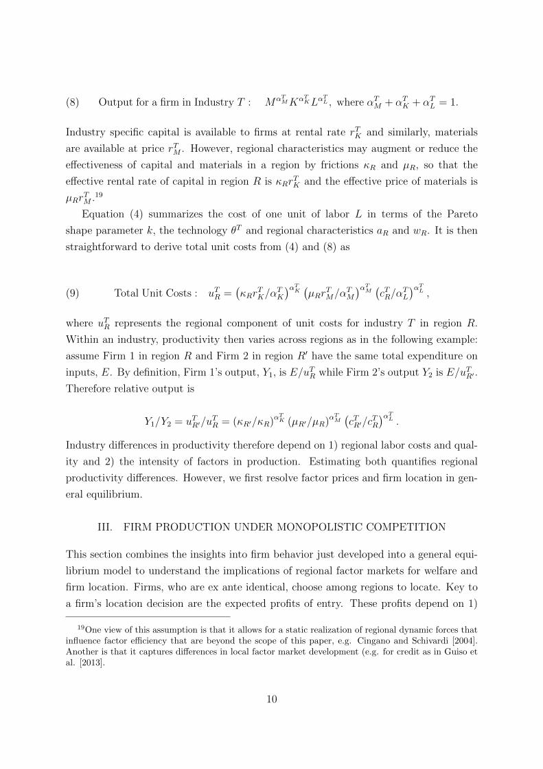
(8) Output for a firm in Industry T : MαTMKαTKLαTL , where αTM + αTK + αTL = 1.

Industry specific capital is available to firms at rental rate rTK and similarly, materials

are available at price rTM . However, regional characteristics may augment or reduce the

effectiveness of capital and materials in a region by frictions κR and µR, so that the

effective rental rate of capital in region R is κRrTK and the effective price of materials is

µRrTM .19

Equation (4) summarizes the cost of one unit of labor L in terms of the Pareto

shape parameter k, the technology θT and regional characteristics aR and wR. It is then

straightforward to derive total unit costs from (4) and (8) as

(9) Total Unit Costs : uTR =(κRr

TK/α

TK

)αTK (µRrTM/αTM)αTM (cTR/αTL)αTL ,where uTR represents the regional component of unit costs for industry T in region R.

Within an industry, productivity then varies across regions as in the following example:

assume Firm 1 in region R and Firm 2 in region R′ have the same total expenditure on

inputs, E. By definition, Firm 1’s output, Y1, is E/uTR while Firm 2’s output Y2 is E/uTR′ .

Therefore relative output is

Y1/Y2 = uTR′/uTR = (κR′/κR)α

TK (µR′/µR)α

TM(cTR′/c

TR

)αTL .Industry differences in productivity therefore depend on 1) regional labor costs and qual-

ity and 2) the intensity of factors in production. Estimating both quantifies regional

productivity differences. However, we first resolve factor prices and firm location in gen-

eral equilibrium.

III. FIRM PRODUCTION UNDER MONOPOLISTIC COMPETITION

This section combines the insights into firm behavior just developed into a general equi-

librium model to understand the implications of regional factor markets for welfare and

firm location. Firms, who are ex ante identical, choose among regions to locate. Key to

a firm’s location decision are the expected profits of entry. These profits depend on 1)

19One view of this assumption is that it allows for a static realization of regional dynamic forces thatinfluence factor efficiency that are beyond the scope of this paper, e.g. Cingano and Schivardi [2004].Another is that it captures differences in local factor market development (e.g. for credit as in Guiso etal. [2013].

10

the regional distribution of worker types and wages, 2) capital and material quality and

3) the competition present from other firms who enter the region. We characterize pro-

duction and location choices conditional on local factor markets. Most strikingly, lower

regional production costs attract more firms for any given technology, which determines

the intensity of economic activity.

Furthermore, we show an equilibrium wage vector exists which supports these choices

by firms for any distribution of labor endowments (e.g. as would be implied by assuming

nominal or real wage equalization across regions). Thus, endowment distributions as

implied by both complete or incomplete labor mobility are consistent with this framework.

Rather than use a macro level model which determines worker location a priori, we will use

micro level population census data to observe the actual composition of labor markets.20

Our goal is to understand how firms optimally respond to local factor markets as they

are, not to predict where workers choose to locate.

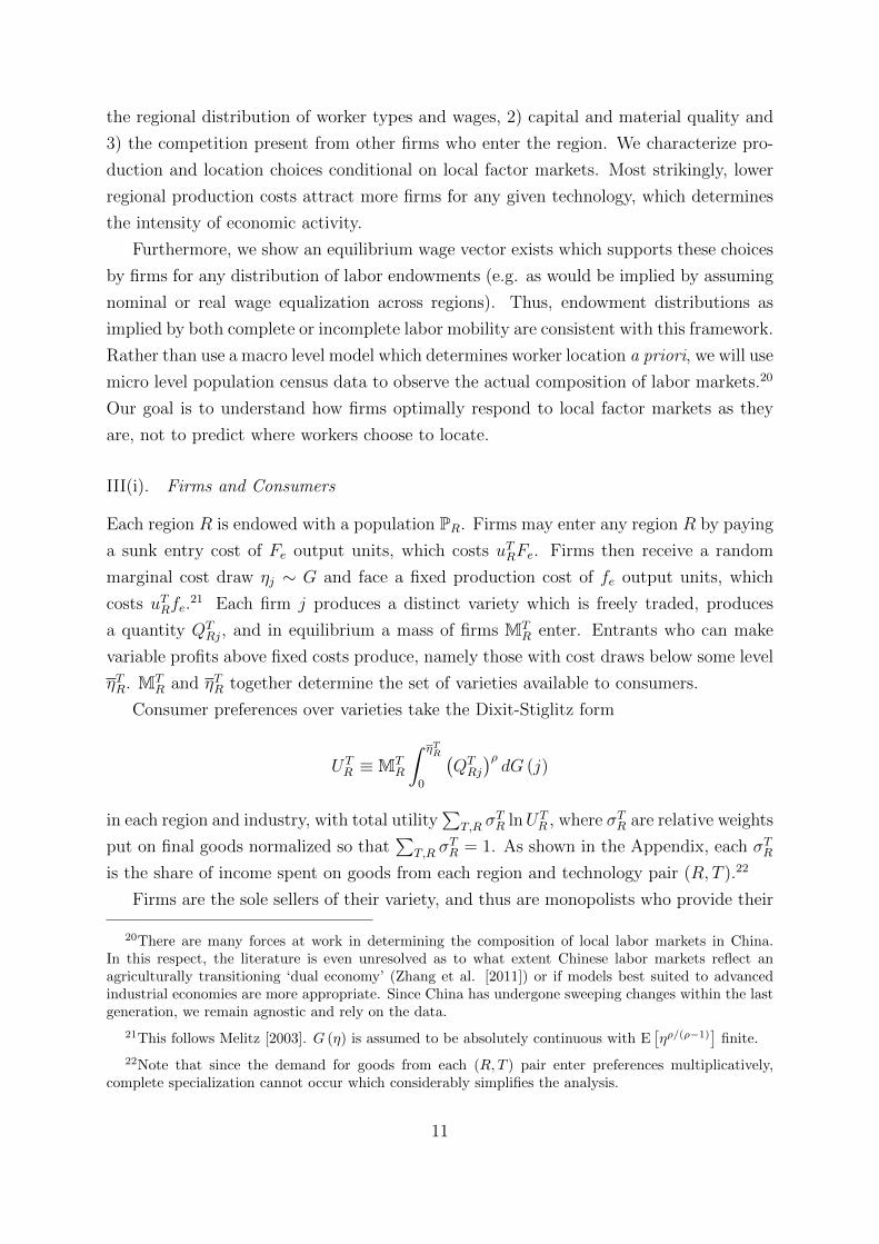
III(i). Firms and Consumers

Each region R is endowed with a population PR. Firms may enter any region R by paying

a sunk entry cost of Fe output units, which costs uTRFe. Firms then receive a random

marginal cost draw ηj ∼ G and face a fixed production cost of fe output units, which

costs uTRfe.21 Each firm j produces a distinct variety which is freely traded, produces

a quantity QTRj, and in equilibrium a mass of firms MT

R enter. Entrants who can make

variable profits above fixed costs produce, namely those with cost draws below some level

ηTR. MTR and ηTR together determine the set of varieties available to consumers.

Consumer preferences over varieties take the Dixit-Stiglitz form

UTR ≡MT

R

∫ ηTR

0

(QTRj

)ρdG (j)

in each region and industry, with total utility∑

T,R σTR lnUT

R , where σTR are relative weights

put on final goods normalized so that∑

T,R σTR = 1. As shown in the Appendix, each σTR

is the share of income spent on goods from each region and technology pair (R, T ).22

Firms are the sole sellers of their variety, and thus are monopolists who provide their

20There are many forces at work in determining the composition of local labor markets in China.In this respect, the literature is even unresolved as to what extent Chinese labor markets reflect anagriculturally transitioning ‘dual economy’ (Zhang et al. [2011]) or if models best suited to advancedindustrial economies are more appropriate. Since China has undergone sweeping changes within the lastgeneration, we remain agnostic and rely on the data.

21This follows Melitz [2003]. G (η) is assumed to be absolutely continuous with E[ηρ/(ρ−1)

]finite.

22Note that since the demand for goods from each (R, T ) pair enter preferences multiplicatively,complete specialization cannot occur which considerably simplifies the analysis.

11

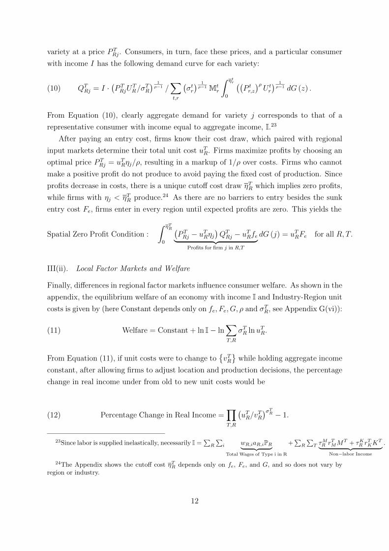
variety at a price P TRj. Consumers, in turn, face these prices, and a particular consumer

with income I has the following demand curve for each variety:

(10) QTRj = I ·

(P TRjU

TR/σ

TR

) 1ρ−1 /

∑t,r

(σtr) 1ρ−1 Mt

r

∫ ηtr

0

((P tr,z

)ρU tr

) 1ρ−1 dG (z) .

From Equation (10), clearly aggregate demand for variety j corresponds to that of a

representative consumer with income equal to aggregate income, I.23

After paying an entry cost, firms know their cost draw, which paired with regional

input markets determine their total unit cost uTR. Firms maximize profits by choosing an

optimal price P TRj = uTRηj/ρ, resulting in a markup of 1/ρ over costs. Firms who cannot

make a positive profit do not produce to avoid paying the fixed cost of production. Since

profits decrease in costs, there is a unique cutoff cost draw ηTR which implies zero profits,

while firms with ηj < ηTR produce.24 As there are no barriers to entry besides the sunk

entry cost Fe, firms enter in every region until expected profits are zero. This yields the

Spatial Zero Profit Condition :

∫ ηTR

0

(P TRj − uTRηj

)QTRj − uTRfe︸ ︷︷ ︸

Profits for firm j in R,T

dG (j) = uTRFe for all R, T.

III(ii). Local Factor Markets and Welfare

Finally, differences in regional factor markets influence consumer welfare. As shown in the

appendix, the equilibrium welfare of an economy with income I and Industry-Region unit

costs is given by (here Constant depends only on fe, Fe, G, ρ and σTR, see Appendix G(vi)):

(11) Welfare = Constant + ln I− ln∑T,R

σTR lnuTR.

From Equation (11), if unit costs were to change to{vTR}

while holding aggregate income

constant, after allowing firms to adjust location and production decisions, the percentage

change in real income under from old to new unit costs would be

(12) Percentage Change in Real Income =∏T,R

(uTR/v

TR

)σTR − 1.

23Since labor is supplied inelastically, necessarily I =∑R

∑i wR,iaR,iPR︸ ︷︷ ︸Total Wages of Type i in R

+∑R

∑T τ

MR rTMM

T + τKR rTKK

T︸ ︷︷ ︸Non−labor Income

.

24The Appendix shows the cutoff cost ηTR depends only on fe, Fe, and G, and so does not vary byregion or industry.

12

Having determined behavior in the product market, we now examine input markets.

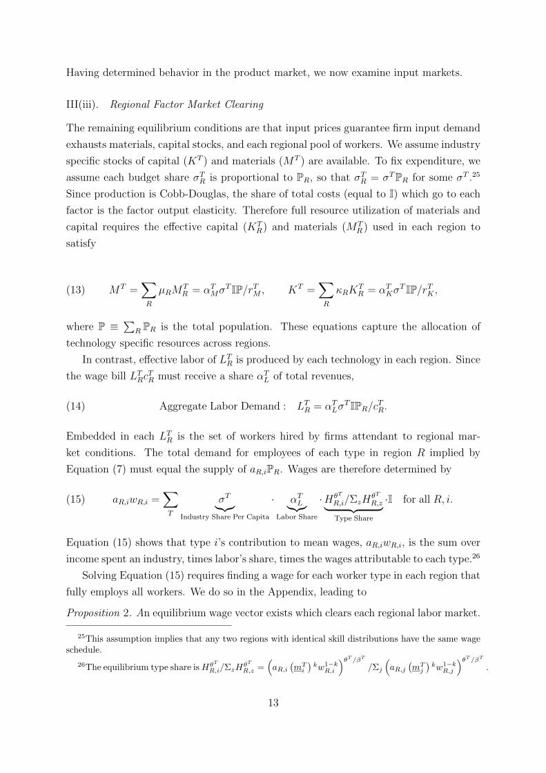
III(iii). Regional Factor Market Clearing

The remaining equilibrium conditions are that input prices guarantee firm input demand

exhausts materials, capital stocks, and each regional pool of workers. We assume industry

specific stocks of capital (KT ) and materials (MT ) are available. To fix expenditure, we

assume each budget share σTR is proportional to PR, so that σTR = σTPR for some σT .25

Since production is Cobb-Douglas, the share of total costs (equal to I) which go to each

factor is the factor output elasticity. Therefore full resource utilization of materials and

capital requires the effective capital (KTR) and materials (MT

R ) used in each region to

satisfy

(13) MT =∑R

µRMTR = αTMσ

T IP/rTM , KT =∑R

κRKTR = αTKσ

T IP/rTK ,

where P ≡∑

R PR is the total population. These equations capture the allocation of

technology specific resources across regions.

In contrast, effective labor of LTR is produced by each technology in each region. Since

the wage bill LTRcTR must receive a share αTL of total revenues,

(14) Aggregate Labor Demand : LTR = αTLσT IPR/cTR.

Embedded in each LTR is the set of workers hired by firms attendant to regional mar-

ket conditions. The total demand for employees of each type in region R implied by

Equation (7) must equal the supply of aR,iPR. Wages are therefore determined by

(15) aR,iwR,i =∑T

σT︸︷︷︸Industry Share Per Capita

· αTL︸︷︷︸Labor Share

·HθT

R,i/ΣzHθT

R,z︸ ︷︷ ︸Type Share

·I for all R, i.

Equation (15) shows that type i’s contribution to mean wages, aR,iwR,i, is the sum over

income spent an industry, times labor’s share, times the wages attributable to each type.26

Solving Equation (15) requires finding a wage for each worker type in each region that

fully employs all workers. We do so in the Appendix, leading to

Proposition 2. An equilibrium wage vector exists which clears each regional labor market.

25This assumption implies that any two regions with identical skill distributions have the same wageschedule.

26The equilibrium type share isHθT

R,i/ΣzHθT

R,z =(aR,i

(mTi

)kw1−k

R,i

)θT /βT

/Σj

(aR,j

(mTj

)kw1−k

R,j

)θT /βT

.

13

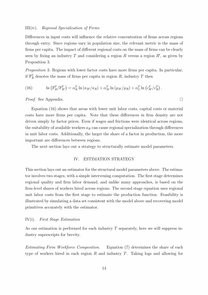
III(iv). Regional Specialization of Firms

Differences in input costs will influence the relative concentration of firms across regions

through entry. Since regions vary in population size, the relevant metric is the mass of

firms per capita. The impact of different regional costs on the mass of firms can be clearly

seen by fixing an industry T and considering a region R versus a region R′, as given by

Proposition 3.

Proposition 3. Regions with lower factor costs have more firms per capita. In particular,

if FTR denotes the mass of firms per capita in region R, industry T then

(16) ln(FTR/FTR′

)= αTK ln (κR′/κR) + αTM ln (µR′/µR) + αTL ln

(cTR′/c

TR

).

Proof. See Appendix.

Equation (16) shows that areas with lower unit labor costs, capital costs or material

costs have more firms per capita. Note that these differences in firm density are not

driven simply by factor prices. Even if wages and frictions were identical across regions,

the suitability of available workers aR can cause regional specialization through differences

in unit labor costs. Additionally, the larger the share of a factor in production, the more

important are differences between regions.

The next section lays out a strategy to structurally estimate model parameters.

IV. ESTIMATION STRATEGY

This section lays out an estimator for the structural model parameters above. The estima-

tor involves two stages, with a simple intervening computation. The first stage determines

regional quality and firm labor demand, and unlike many approaches, is based on the

firm-level shares of workers hired across regions. The second stage equation uses regional

unit labor costs from the first stage to estimate the production function. Feasibility is

illustrated by simulating a data set consistent with the model above and recovering model

primitives accurately with the estimator.

IV(i). First Stage Estimation

As our estimation is performed for each industry T separately, here we will suppress in-

dustry superscripts for brevity.

Estimating Firm Workforce Composition. Equation (7) determines the share of each

type of workers hired in each region R and industry T . Taking logs and allowing for

14

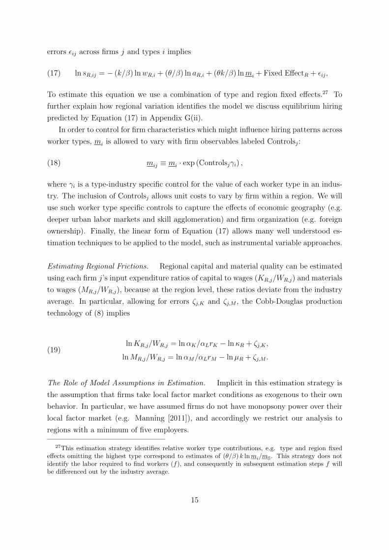
errors εij across firms j and types i implies

(17) ln sR,ij = − (k/β) lnwR,i + (θ/β) ln aR,i + (θk/β) lnmi + Fixed EffectR + εij,

To estimate this equation we use a combination of type and region fixed effects.27 To

further explain how regional variation identifies the model we discuss equilibrium hiring

predicted by Equation (17) in Appendix G(ii).

In order to control for firm characteristics which might influence hiring patterns across

worker types, mi is allowed to vary with firm observables labeled Controlsj:

(18) mij ≡ mi · exp (Controlsjγi) ,

where γi is a type-industry specific control for the value of each worker type in an indus-

try. The inclusion of Controlsj allows unit costs to vary by firm within a region. We will

use such worker type specific controls to capture the effects of economic geography (e.g.

deeper urban labor markets and skill agglomeration) and firm organization (e.g. foreign

ownership). Finally, the linear form of Equation (17) allows many well understood es-

timation techniques to be applied to the model, such as instrumental variable approaches.

Estimating Regional Frictions. Regional capital and material quality can be estimated

using each firm j’s input expenditure ratios of capital to wages (KR,j/WR,j) and materials

to wages (MR,j/WR,j), because at the region level, these ratios deviate from the industry

average. In particular, allowing for errors ζj,K and ζj,M , the Cobb-Douglas production

technology of (8) implies

(19)lnKR,j/WR,j = lnαK/αLrK − lnκR + ζj,K ,

lnMR,j/WR,j = lnαM/αLrM − lnµR + ζj,M .

The Role of Model Assumptions in Estimation. Implicit in this estimation strategy is

the assumption that firms take local factor market conditions as exogenous to their own

behavior. In particular, we have assumed firms do not have monopsony power over their

local factor market (e.g. Manning [2011]), and accordingly we restrict our analysis to

regions with a minimum of five employers.

27This estimation strategy identifies relative worker type contributions, e.g. type and region fixedeffects omitting the highest type correspond to estimates of (θ/β) k lnmi/mS. This strategy does notidentify the labor required to find workers (f), and consequently in subsequent estimation steps f willbe differenced out by the industry average.

15

Since we are explaining firm hiring behavior in response to exogenous local market

conditions, one endogeniety concern might be that regional factors simultaneously shift

the supply or wages of manufacturing workers and individual firm demand across worker

types. Accordingly, below we implement an instrumental variables strategy to address

this potential source of endogeniety and assess the robustness of the estimates.

Finally, the estimates of unit labor costs and regional frictions for capital and materials

are completely distinct and do not rely on estimates of each other. However, all of them

together influence the estimation of substitution between these three inputs, which we

now detail.

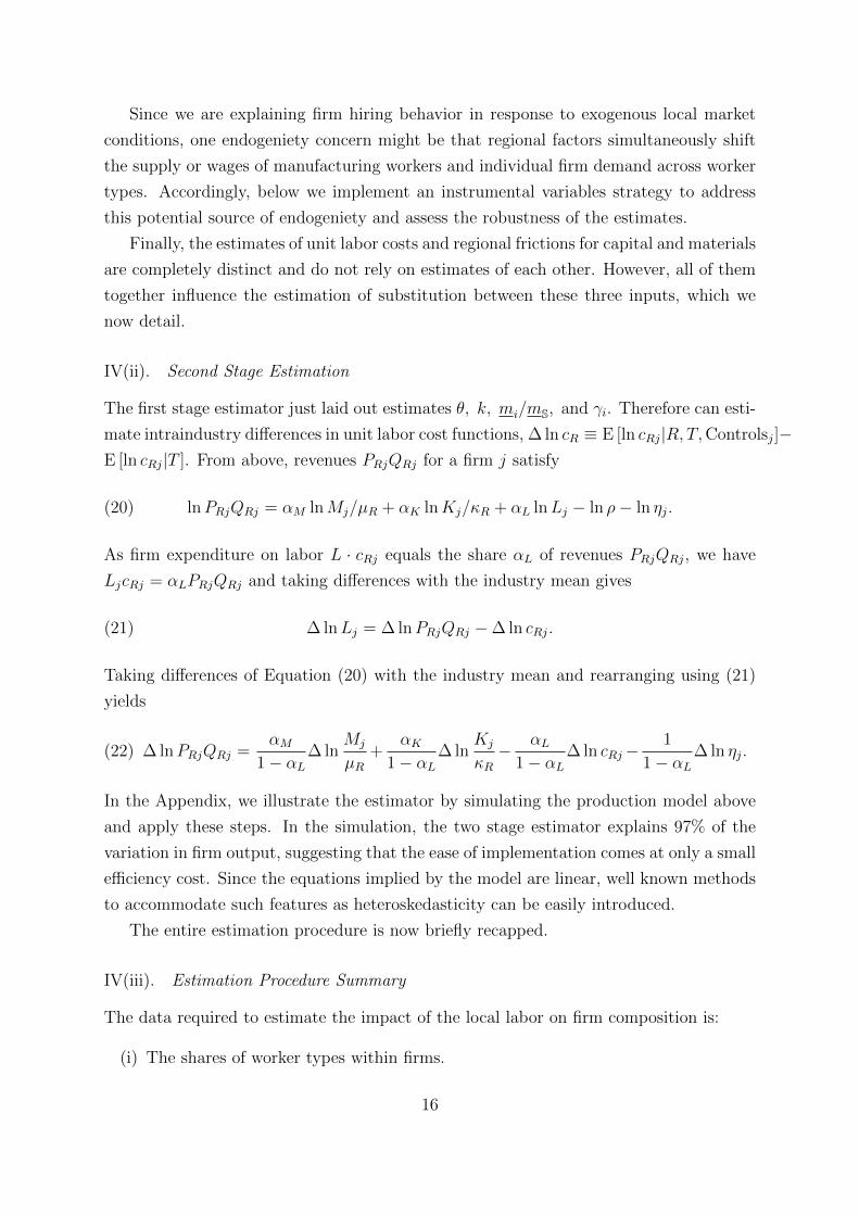
IV(ii). Second Stage Estimation

The first stage estimator just laid out estimates θ, k, mi/mS, and γi. Therefore can esti-

mate intraindustry differences in unit labor cost functions, ∆ ln cR ≡ E [ln cRj|R, T,Controlsj]−E [ln cRj|T ]. From above, revenues PRjQRj for a firm j satisfy

(20) lnPRjQRj = αM lnMj/µR + αK lnKj/κR + αL lnLj − ln ρ− ln ηj.

As firm expenditure on labor L · cRj equals the share αL of revenues PRjQRj, we have

LjcRj = αLPRjQRj and taking differences with the industry mean gives

(21) ∆ lnLj = ∆ lnPRjQRj −∆ ln cRj.

Taking differences of Equation (20) with the industry mean and rearranging using (21)

yields

(22) ∆ lnPRjQRj =αM

1− αL∆ ln

Mj

µR+

αK1− αL

∆ lnKj

κR− αL

1− αL∆ ln cRj−

1

1− αL∆ ln ηj.

In the Appendix, we illustrate the estimator by simulating the production model above

and apply these steps. In the simulation, the two stage estimator explains 97% of the

variation in firm output, suggesting that the ease of implementation comes at only a small

efficiency cost. Since the equations implied by the model are linear, well known methods

to accommodate such features as heteroskedasticity can be easily introduced.

The entire estimation procedure is now briefly recapped.

IV(iii). Estimation Procedure Summary

The data required to estimate the impact of the local labor on firm composition is:

(i) The shares of worker types within firms.

16

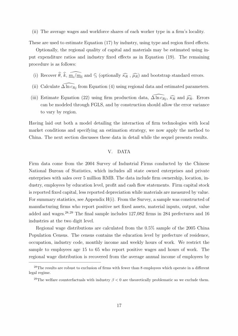
(ii) The average wages and workforce shares of each worker type in a firm’s locality.

These are used to estimate Equation (17) by industry, using type and region fixed effects.

Optionally, the regional quality of capital and materials may be estimated using in-

put expenditure ratios and industry fixed effects as in Equation (19). The remaining

procedure is as follows:

(i) Recover θ, k, mi/mS and γi (optionally κR , µR) and bootstrap standard errors.

(ii) Calculate ∆ ln cRj from Equation (4) using regional data and estimated parameters.

(iii) Estimate Equation (22) using firm production data, ∆ ln cRj, κR and µR. Errors

can be modeled through FGLS, and by construction should allow the error variance

to vary by region.

Having laid out both a model detailing the interaction of firm technologies with local

market conditions and specifying an estimation strategy, we now apply the method to

China. The next section discusses these data in detail while the sequel presents results.

V. DATA

Firm data come from the 2004 Survey of Industrial Firms conducted by the Chinese

National Bureau of Statistics, which includes all state owned enterprises and private

enterprises with sales over 5 million RMB. The data include firm ownership, location, in-

dustry, employees by education level, profit and cash flow statements. Firm capital stock

is reported fixed capital, less reported depreciation while materials are measured by value.

For summary statistics, see Appendix H(i). From the Survey, a sample was constructed of

manufacturing firms who report positive net fixed assets, material inputs, output, value

added and wages.28,29 The final sample includes 127,082 firms in 284 prefectures and 16

industries at the two digit level.

Regional wage distributions are calculated from the 0.5% sample of the 2005 China

Population Census. The census contains the education level by prefecture of residence,

occupation, industry code, monthly income and weekly hours of work. We restrict the

sample to employees age 15 to 65 who report positive wages and hours of work. The

regional wage distribution is recovered from the average annual income of employees by

28The results are robust to exclusion of firms with fewer than 8 employees which operate in a differentlegal regime.

29The welfare counterfactuals with industry β < 0 are theoretically problematic so we exclude them.

17

education using census data.30

GIS data from the China Data Center at the University of Michigan locates firms

at the county and prefecture level. Port locations are provided by GIS data and sup-

plemented by data from the World Port Index. These data provide controls for urban

status, distance to port, highway density and distance to cities.

Finally, welfare calculations rely on household consumption shares for each industry

are aggregated from the three digit level from the 2002 Input-Output Table of China,

as constructed by the Department of National Economy Accounting, State Statistical

Bureau.

Figure 2a illustrates the prefectures of China, which we define as regions from the

perspective of the model above. Prefectures are similar in population size to a US com-

muting zone, as used by Autor et al. [2013] and computed by Tolbert and Sizer [1996].

Prefectures illustrated by a darker shade in the Figure operate under substantially dif-

ferent government policies and objectives. These regions typically have large minority

populations or historically distinct conditions, with the majority declared as autonomous

regions, and have idiosyncratic regulations, development, and educational policies. We

exclude the five Autonomous Provinces and one predominantly minority Province (Qing-

hai) which has a very low density of population and economic activity.31 What remains

are the lighter shaded regions of Figure 2a, preserving 284 prefectures displaying distinct

labor market conditions.

Place Figure 2 about here.

V(i). Worker Types

Workers are defined as people between ages 15 and 65 who work outside the agricultural

sector and are not employers, self-employed, or in a family business. This character-

ization includes migrants. The definition of distinct, imperfectly substitutable worker

types is based primarily on formal schooling attained. Census data from 2005 shows that

the average years of schooling for workers in China ranges from 8.5 to 11.8 years across

provinces, with sparse postgraduate education. The most common level of formal educa-

tion is at the Junior High School level or below. Reflecting substantial wage differences

by gender within that group, we define Type 1 workers as Junior High School or Below:

30While firm data is from 2004 and census data is from 2005, the limited evidence on firm skill mixis that it is remarkably stable over time: Ilmakunnas and Ilmakunnas [2011] find the standard deviationof plant-level education years is very stable from 1995-2004 in Finland, and Parrotta et al. [2011] findthat a firm-level education diversity index was roughly constant over a decade in Denmark.

31See the Information Office of the State Council of the People’s Republic of China document cited.

18

Female and Type 2 workers as Junior High School or Below: Male.32 Completion of

Senior High School defines Type 3 and completion of Junior College or Higher Education

defines Type 4.

V(ii). Regional Variation

Key to the analysis is regional variation in skill distribution and wages. Here we briefly

discuss both, with further details in Appendix G(vii). While this paper explains individ-

ual firms’ responses to existing labor market conditions rather than providing a theory of

worker location, it is clear that the recent history of China has exhibited massive internal

migration (Chan [2013]).33 Monthly incomes vary substantially across China as illus-

trated in Figure 2b. This is due to both the composition of skills (proxied by education)

across regions and the rates paid to these skills. Figure 3 contrasts educational distribu-

tions of the labor force. Figure 3a shows those with a Junior High School education (the

mandated level in China), while Figure 3b displays those with a Junior College or higher

level of attainment.

Place Figure 3 about here.

The differing composition of input markets across China in 2004-2005 stem from

many factors, including the dynamic nature of China’s rapidly growing economy, targeted

economic policies and geographic agglomeration of industries across China.34 Faber [2014]

finds that expansion of China’s National Trunk Highway System displaced economic

activity from counties peripheral to the System. Similarly, Baum-Snow et al. [2017]

show that mass transit systems in China have increased the population density in city

centers, while radial highways around cities have dispersed population and industrial

activity. An overview of Chinese economic policies is provided by Defever and Riano

[2017], who quantify their impact on firms.

Of particular interest for labor markets are substantial variation in wages and the at-

tendant migration this induces. The quantitative extent to which labor market migration

32Differentiation of gender for low skill labor is especially important in developing countries as avariety of influences result in imperfect substitutability across gender. Bernhofen and Brown [2016]distinguish between skilled male labor, unskilled male labour and female labour and find that the factorprices across these types differ substantially.

33In 2005, the median share of within prefecture migration is 77%, dominating across prefecturemigration.

34We consider regional price variation at a fixed point in time. Reallocation occurs (Ge and Yang[2014]) and is important in explaining dynamics (e.g. Borjas [2003]), but dynamics are outside the scopeof this paper.

19

has been stymied by the hukou system of internal passports is not well studied, although

its impact has likely lessened since 2000.35 Since little is known about the impact of

illegal immigration on firm behavior (see Brown et al. [2013] for a notable exception),

and as the ease of obtaining a legal hukou is not independent of education,36 we control

for the regional share of non-agricultural hukou held by each type of worker without any

a priori expectation of sign. Given that rural to urban migration typifies the pattern of

structural transformation underway, we control for rural and urban effects for each type

of worker below. While modeling dynamic worker considerations is beyond the scope of

this paper, presumably the dynamic forces that impact the manufacturing labor force

would similarly impact the service sector labor force, and accordingly we re-estimate the

structural parameters instrumenting manufacturing labor market conditions with service

sector labor market conditions as reported by the Population Census sample.

Having discussed the data, we now apply the estimation procedure developed above.

VI. ESTIMATION RESULTS

This section reports estimation results, then turns to a discussion of the quantitative labor

cost and productivity differences accounted for by local market conditions in China. The

section continues by comparing the ability of the model to explain productivity differences

with this unit cost based method with one approach common in the literature, which does

not account for regional factor markets and models labor types as input stocks. We then

quantify the importance of the estimated productivity differences for welfare by using

the general equilibrium model to consider a hypothetical Chinese economy in which the

distribution of workers and wages across regions is equalized. Finally, we test the firm

location implications of the model, finding support that economic activity locates where

estimated unit labor costs are lower.

VI(i). Estimates of Market Conditions and Production Technologies

The full first stage regression results for several manufacturing industries in China are

presented in Tables IX and X of Appendix B(i). A representative set of estimates for the

General Machines industry are presented in Table I. The first box in Table I, labeled

Primary Variables, are consistent with the model: increases in the local wages for a type

decrease firm demand for that type, while increases in the availability of a type increase

35The Hukou system and its reform in the late 1990s are well explained in Chan and Buckingham[2008]. The persistence of such a stratified system has engendered deep set social attitudes which likelyaffect economic interactions between Hukou groups, see Afridia et al. [2015].

36High income and highly educated workers can more easily move among urban regions as localgovernments are likely to approve their migration applications (Chan et al. [1999]).

20

firm demand.37 Though values for the coefficients(θT/βT

)lnmT

i /mT4 are not specified

by the model, their estimated values do increase in type in Table I, which is consonant

with formal education increasing worker output.

The remaining two boxes include regional controls from the Census and firm level

controls from the manufacturing survey. The regional controls are by prefecture, and in-

clude the percentage of each type with a non-agricultural Hukou. The firm level controls

include the share of foreign equity, whether the firm is in an urban area, and the age of

the firm. Most interestingly, firms in urban areas or with higher shares of foreign equity

tend to have increasingly higher demand for higher skilled workers, as evidenced by the

increasing pattern of coefficients across worker types.38

Place Table I about here.

Inclusion of controls for average worker age, which control for accumulated skill or

vintage human capital, do not appreciably alter the results. Other controls which did not

appreciably alter the results include state ownership39, distance to port, firm size and the

percentage of migrants in a region.

Explanatory Importance of Local Worker Availability versus Wages. One innovation of

the model and empirical strategy is to estimate and quantify the role of local worker avail-

ability in firm hiring decisions. While this is novel, its empirical relevance is supported

by both the significance of the coefficients on worker availability (Tables IX and X), but

also by the higher explanatory value of worker availability. This is demonstrated in Fig-

ure 4, which displays the R2 of regressions by industry using the specification of Table I

in black, and the corresponding R2 for the same specification omitting availability (light

grey) or wages (dark grey). In almost every industry, worker availability explains more

firm workforce variation than wages.40

Place Figure 4 about here.

37This second result is in line with recent findings on firm and industry responses to changes in laborsupply of Gonzlez and Ortega [2011] and Dustmann and Glitz [2015].

38The latter of these two patterns is supported by estimates of the skill composition in Swedish firmsby Davidson et al. [2013].

39The industries with the highest shares of state ownership, Printing and Transport, were censoredover concerns regarding hiring incentives and geographic location. Both industries are relatively capitalintensive, so that labor market effects are of secondary importance.

40Bootstrapping the sample shows we can reject the hypothesis that the R2 of the wage regressionsis higher than the R2 of the availability regressions at the 95% confidence level in 13 of 16 industries.

21

Differences in Production Costs by Region These first stage estimates are interesting

in themselves, as the model then implies the unit cost function for labor by region. The

dispersion of estimated unit labor costs in the General Machines industry are depicted

in Figure 5. As General Machines is an industry with θT > 1, low cost areas (light grey)

represent areas with a combination of not only low wages, but deep pools of similar types

of workers.

Place Figure 5 about here.

Other features of regional factor markets might influence the relative quality of capital

and materials to labor, such as the depth of input/output markets, infrastructure or

agglomerative forces. To control for these features, we use Equation (19) to estimate

regional capital and material quality using the distance from the center of each firm’s

county to the nearest large city, arriving at

lnκR = 0.315(0.096)

·Distance to City (per 100 km) + Industry Fixed Effect,

lnµR = 0.236(0.123)

·Distance to City (per 100 km) + Industry Fixed Effect.

The model primitives of the two stage estimation procedure across industries are

summarized in Table II. Standard errors are calculated using a bootstrap stratified on

industry and region, since these estimates rely on the first stage estimates of structural

model parameters. Table II displays the estimated model primitives, showing a range of

significantly different technologies θT and match quality distributions through k. Table

II also shows the second stage estimation results, where the regional unit labor costs are

calculated using regional data and the first stage estimates.41

Place Table II about here.

While the capital coefficients may seem low, they are not out of line with other

estimates which specifically account for material inputs (e.g. Javorcik [2004]). For the

41These second estimates include controls for the percentage of female and white collar workers,percentage of state and foreign equity, share of revenues exported and the logarithm of the age of thefirm.

22

specific case of China, there are few comparable studies.42,43

In comparison with our findings, Brandt et al. [2012] estimate the total factor pro-

ductivity of Chinese manufacturing firms in 1998-2007 using both the Olley-Pakes and

Ackerberg-Caves-Frazer estimation methods. Their results suggest that there are de-

creasing returns to scale in almost all industries in China. Their average sum of input

intensities are 0.8 for Olley-Pakes and 0.7 for Ackerberg-Caves-Frazer, and the average

sum of input intensities in our case is 0.8, in line with their higher range. Brandt et

al. argue that measurement error and price setting power are plausible explanations for

the low estimates, although this issue is not addressed in their paper due to the lack of

firm-level price information (e.g. using the method of De Loecker [2011]), a limitation we

also face.

Robustness: Instrumenting Manufacturing Labor Market Conditions To address po-

tential simultaneity issues between the relative demand for worker types and the local

supply or wages of workers, we instrument worker wages and availability (wR,i and aR,i)

by service sector wages, unemployment and workforce shares. While outside the scope of

our model, the idea here is that service sector workers are likely somewhat mobile into

manufacturing employment and thus service sector labor market conditions are likely cor-

related with those in manufacturing. However, it is unlikely that aggregate labor market

conditions in the service sector would influence individual manufacturing firm’s workforce

decisions beyond the effects they have on manufacturing wages and availability. The re-

sults (see Appendix) do not drastically change the point estimates of structural model

parameters which are the basis for our subsequent analysis, while the standard errors of

structural estimates increase.

Robustness: Firm Size and Input Complementarity As the optimal distribution of

worker types within a firm might change with firm size, and because different worker

types might have different complementarities with other inputs such as capital and ma-

terials, we have run two robustness checks of our first stage. The first check interacts

each worker type with the logarithm of the number of employees as a measure of firm

42Though not directly comparable, macroeconomic estimates include Chow [1993] and Ozyurt [2009]who find higher capital coefficients. These studies do not account for materials. The most comparablestudy is Fleisher and Wang [2004] who find microeconomic estimates for αK in the range of .40 to .50(they do not differentiate between capital and materials) and this compares favorably with the combinedestimates of αK + αM in Table II.

43We interpret the second stage estimates for Textiles with caution as capital and materials may haveincreased in anticipation of the Multifibre Arrangement expiring in 2005, at the end of which Chineseexports grew by over 100% in many categories. We have excluded the Apparel and Man-Made Fibreindustries for this reason as they additionally fail the model restriction β ≥ 0.

23

size (reported in the third and fourth column of Table XVI, see Appendix). The second

check interacts each worker type with capital and material intensity as measured by the

logarithm of capital and materials per worker (reported in the fifth and sixth column of

Table XVI, see Appendix). The estimates are robust to these extended specification: the

changes in estimates are small and generally not significant, as seen by comparing the

results with the baseline specification of Table XVI in the first and second columns.

Robustness: Unobserved Regional Heterogeneity One potential concern is bias in the

second stage due to omitted variables which influence input usage across regions separate

from our model or observable controls. To address this, following the productivity esti-

mation literature and noting that among inputs, capital stocks are likely slower to adjust

to idiosyncratic differences (e.g. productivity, prices) than material and labor inputs, we

adopt a prefecture-industry level IV strategy. We instrument firm level unit labor costs

and the logarithm of material costs using the average unit labor cost and average (log)

material costs at the prefecture-industry level. The second stage estimates, which allow

us to quantify the productivity differences implied by the unit labor costs, are broadly

similar (for a comparison, see Table XVII in the Appendix).

VI(ii). Implied Productivity Differences Across Firms

Table III quantifies the implied differences in unit labor costs. The cTR column displays

the interquartile (75%/25%) unit labor cost ratios by industry where unit labor costs have

been calculated according to the model, and range from about 30 to 80% cost differences

within industry. The(cTR)αTL column takes into account substitution into non-labor inputs

and range from about 3 to 12%. For example, consider two firms in General Machines

at the 25th and 75th unit labor cost percentile. If both firms have the same wage bill,

the labor (L) available to the lower cost firm is 1.41 times greater than the higher cost

firm. From Table II above, the estimated share of wages in production is αTL = 0.17, so

the lower cost firm will produce 1.41.17 = 1.06 times as much output as the higher cost

firm, holding all else constant.

Place Table III about here.

Table III indicates that the range of total unit costs faced by firms within the same

industry are indeed substantial, even after explicitly taking into account the technology

θT and the ability to substitute across several types of local workers. However, the second

stage estimates indicate these differences are attenuated by substitution into capital and

materials. Thus, while differences in regional markets indicate an interquartile range

24

of 30-80% in unit cost differences, substitution into other factors reduces this range to

between 3-12%.

Table IV displays similar calculations for capital and materials. The καTKR and µ

αTMR

columns display the interquartile ratio of capital and material quality, ranging from about

1 to 3% for capital and 2 to 5% for materials. Clearly estimated differences in labor mar-

kets are substantially wider, in part due to the fact that we observe more information

about workers than types of capital or materials. Finally, the uTR column contains the

differences in productivity implied by regional cost differences as laid out in Section II(iv).

Place Table IV about here.

Table V examines the variance of productivity by industry under the unit cost method

(Column 1) compared to estimating output by a Cobb-Douglas combination of capital,

materials and the number of each worker type (Column 2). Column 3 of Table V shows

the average percentage that unexplained productivity is reduced per firm under the unit

labor cost method.44 As shown by the Table, the variance of unexplained productiv-

ity is reduced by about 6 to 30% once local factor markets are explicitly accounted for,

showing that this approach does indeed provide more information about the determinants

of firm productivity, with the relative importance of inputs indicated by Tables III and IV.

Place Table V about here.

We next quantify the net impact of these productivity differences across China by

evaluating the change in real income consumers would experience if labor markets were

homogeneous.

VI(iii). Consumer Welfare and Local Factor Market Costs

We now consider a hypothetical Chinese economy in which the distribution of workers

and wages across regions is equalized to the national average for each worker type. This

is of course an unrealistic assumption given the myriad influences of workers’ location

decisions, but does provide a benchmark to quantify the welfare impacts of homogenizing

labor costs across China, and thus the importance of factor markets.

Letting{uTR}

be the estimated unit costs for China, PR the population of manufac-

44Most models used in production estimation assume perfect labor substitutability. Such modelsimply that, conditional on wages, the local composition of the workforce is irrelevant for hiring. Theapproach of this paper incorporates local factor supply and an empirical comparison with other modelsis presented in Appendix C(ii).

25

turing workers in region R and σT the share of consumption for each industry T as given

by the 2002 Input-Output Tables for China, Equation (12) can be computed for new unit

costs{vTR}

. To arrive at{vTR}

, we use our model parameter estimates while assuming

that each region contains the nationally averaged frequency of each worker type who re-

ceives the nationally averaged wage for their type. This implies a more even distribution

of worker types and wages that will reallocate expenditure across regions and industries

in potentially advantageous ways. In particular, more firms will enter into areas where

costs drop and will exit areas where costs rise. Calculation of Equation (12) yields a real

income gain of 1.33% under our baseline estimates, and 1.11% under our instrumental

variables estimates.45 This suggests that while factor market differences are large, if firms

relocate in response to these new conditions as in our model, the net welfare gains are in

line with other estimates of the gains from trade for large countries.

Since firms locate freely, the model predicts that these substantial cost differences

drive economic activity towards more advantageous locations, which we now examine.

VI(iv). Aggregate Firm Location

Per capita volumes of economic activity across regions are determined by Equation (16),

which states that relatively lower industry labor costs should attract relatively more firms

to a region. Due to a lack of panel data or instruments which might convincingly ad-

dress confounding empirical issues such as the role of Chinese industrial policy or the

joint determination of firm and worker location (beyond the relationships explained by

the model), we interpret our results as a quantification of model relationships, rather

than a causal relationship. Table VI summarizes estimates of this relationship, control-

ling for regional distance to the nearest city (weighted by the share of log value added

in a region).46 A firm’s distance from a city may explain many factors, and above we

have seen firms closer to cities have relatively higher capital and material quality. Even

controlling for geography, the impact of advantageous labor markets still often remains.

Whenever the relationship between value added and labor costs is statistically significant,

the relationship is negative, in line with the model.47 While the point estimates vary, the

median significant estimate is about -0.7, indicating a 10% increase in unit labor costs is

associated with an 7% decrease in value added per capita.

45Since unit costs in fact vary at the firm level, we use the employment weighted average of firm unitcosts in each region-industry pair.

46Rizov and Zhang [2013] find that aggregate productivity is higher in regions with high populationdensity, and the theory of this paper implies productivity drives increased entry.

47These results are robust if distance is unweighted, and to the inclusion of Economic Zone status.

26

Place Table VI about here.

VI(v). Labor Markets and China’s WTO Accession

As a counterfactual exercise, we consider the impact of improved access to US mar-

kets arising from a structural shift in trade policy, namely China’s WTO membership

in 2001. China’s permanent normal trade relations with the US reduced the expected

tariffs faced by Chinese exporters in the face of potential non-renewal of MFN status

by the US Congress (see Pierce and Schott [2016] for more details).48 We measure the

effect of this policy change on labor markets at the prefecture level, for all prefectures

which have obtained ‘city’ status (207 prefectures) and therefore appear in both the 1999

China City Statistical Yearbook and 1998 Annual Industrial Survey. This allows us to

aggregate the reduction in expected tariffs at the prefecture level using the Bartik (1991)

composition method. We construct a 4 digit ISIC tariff gap measure for each industry

T , TariffGapT ,49 and weight the impact of TariffGapT by the employment share of each

industry in prefecture R in 1998 to arrive at the regional treatment

TariffGapRegionR ≡∑T

Employment ShareTR · TariffGapT .

We use TariffGapRegionR to predict changes in the population share of worker types in

each region between 2000 and 2005 due to WTO accession using local linear estimates as

presented in Figure 8 of the Appendix.50

We use the predicted population share changes to predict the skill distribution of

prefectures if China had not acceded to the WTO. We then recalculate the unit labor costs

and productivity for each firm and compare the dispersion of these counterfactuals with

the actual dispersion as presented in Table XVIII of the Appendix.While the interquartile

unit cost ratios do vary slightly under the two scenarios, the interquartile productivity

ratios are essentially identical across the two scenarios.51 There are only slightly larger

differences at the 90/10 and 95/5 percentiles, indicating that while skill distributions of

workers were effected by China’s WTO accession, relative productivity distributions of

48Pierce and Schott [2016] argue that US tariff gaps are plausibly exogenous to outcomes in China as89% of the variation in tariff gap is from the variation in Smoot-Hawley tariffs which were set 70 yearsprior to China’s WTO accession.

49Defined as the simple average of HS- 6 product-level tariff gaps averaged to the 4 digit ISIC level,using the UN Statistics concordance.

50Note we have no wage data by type for the year 2000 so have no similar way of performing acounterfactual for wages by type.

51With the exception of the Iron and Steel sector which has an interquartile productivity ratio of 1.15vs 1.14 under trade policy uncertainty.

27

firms were essentially unchanged.

VII. CONCLUSION

This paper examines the importance of local supply characteristics in determining firm

input usage and productivity. To do so, a theory and empirical method are developed

to identify firm input demand across industries and heterogeneous labor markets. The

model derives labor demand as driven by the local distribution of wages and available

skills. Firm behavior in general equilibrium is derived, and determines firm location as a

function of regional costs. This results in an estimator which can be easily implemented

in two steps. The first step exploits differences in firm hiring patterns across distinct

regional factor markets to recover firm labor demand by type, and similarly, differences

in regional factor quality. These estimates quantify local unit labor costs and combine

otherwise disparate data sets on firms and labor markets into a unified framework. The

second step introduces local factor market costs into production function estimation.

Both steps characterize the impact of local market conditions on firm behavior through

recovery of model primitives. This is of particular interest when explaining the relative

productivity or location of firms, especially in settings where local characteristics are

highly dissimilar.

Applying the model framework to China, which possesses a large number of distinct

and varied factor markets shows this approach uncovers substantial determinants of firm

heterogeneity. Estimates imply an interquartile difference in labor costs of 30 to 80% and

productivity differences of 3 to 12%. Differences in capital and material quality explain

similar interquartile differences. The results illustrate that local factor market conditions

explain substantial differences in firm workforce composition, input use and productivity.

This is underscored by the estimate that complete homogenization of labor markets would

lead to a 1.33% increase in real income for Chinese consumers as firms adapt to local

factor market conditions. In addition, the variance of unexplained productivity is reduced

by 6 to 30% compared to a standard estimation approach which does not account for

local factor markets. Modeling a firm’s local environment yields substantial insights into

production patterns that are quantitatively important.

The importance of local factor markets for understanding firm behavior suggests new

dimensions for policy analysis. For instance, regions with labor markets which generate

lower unit labor costs tend to attract higher levels of firm activity within an industry. As

unit labor costs depend on rather the distribution of wages and worker types that rep-

resent substitution options, this yields a deeper view of how educational policy or flows

of different worker types impact firms. For this reason, work evaluating wage determi-

28

nation could be enriched by taking this approach.52 Taken as a whole, the results show

that policy changes which influence the composition of regional labor markets will likely

have sizable effects on firm productivity and location. Finally, the substantial differences

within industry suggest that at the regional level, inherent comparative advantages exist

which policymakers might leverage.53

Furthermore, as pointed out by Ottaviano and Peri [2013], little is known about the

dynamic relationships between labor markets and firm behavior, and this paper provides

both a general equilibrium theory and structural estimation strategy to evaluate these

linkages.54 Having seen that cost and productivity differences inherent in local factor

markets are potentially large, our approach could be of use in evaluating trade offs be-

tween regional policies or ongoing trends across regions. Finally, nothing precludes the

application of this paper’s approach beyond China, and it is suitable for analyzing regions

which exhibit a high degree of labor market heterogeneity. Further work could leverage or

extend the approach of combining firm, census and geographic data to better understand

the role of local factor markets on firm behavior.

52There is large literature following Hellerstein et al. [1999]. For instance, Biesebroeck [2011] find theusual relationship between wages and marginal productivity breaks down in less developed countries.Investigating this relationship using our approach could shed light on regional determinants of labormarket clearing, for instance evaluating gender differentials as in Dong and Zhang [2009].

53For a discussion of broader policy implications of regional differences in production, see Luger andEvans [1988].

54Early results suggest firm entry is responsive to labor market changes, especially in manufacturing(Olney [2013]), and labor costs are known to strongly influence vertical production networks (Hanson etal. [2005]).

29

REFERENCES

Abowd, J. M., Haltiwanger, J., Jarmin, R., Lane, J., Lengermann, P., McCue, K., McK-

inney, K. and Sandusky, K., 2005, ‘The Relation among Human Capital, Productivity,

and Market Value: Building Up from Micro Evidence’, in Corrado,C., Haltiwanger, J.,

and Sichel, D. (eds), Measuring Capital in the New Economy (National Bureau of Eco-

nomic Research, U.S.A)

Abowd, J. M., Kramarz, F. and Margolis, D. N., 1999, ‘High Wage Workers and High

Wage Firms’, Econometrica, 67(2), pp. 251-333.

Afridia, F., Xin, S. and Ren, Y., 2015, ‘Social Identity and Inequality: The Impact

of China’s Hukou System’, Journal of Public Economics, 124, pp. 12-29.

Atalay, E., Hortacsu, A. and Syverson, C., 2012, ‘Why Do Firms Own Production

Chains?’, NBER Working Paper 18020.

Autor, D. H., Dorn, D. and Hanson, G. H., 2013, ‘The China Syndrome: Local Labor

Market Effects of Import Competition in the United States’, The American Economic

Review, 103(6), pp. 2121-2168.

Bandiera, O., Barankay, I. and Rasul, I., 2009, ‘Social Connections and Incentives in

the Workplace: Evidence from Personnel Data’, Econometrica, 77(4), pp. 1047-1094.

Bartik, T. J., 1991, Who Benefits from State and Local Economic Development Poli-

cies?, (Upjohn Press, Kalamazoo, U.S.A.)

Bas, M. and Strauss-Kahn, V., 2012, ‘Input-trade Liberalization, Export Prices and

Quality Upgrading’, Journal of International Economics, 95(2), pp. 250262.

Baum-Snow, N., Brandt, L., Henderson, J. V., Turner, M. A. and Zhang, Q., 2017,

‘Roads, Railroads and Decentralization of Chinese Cities’, Review of Economics and

Statistics, 99(3), pp. 435-448.

Bernard, A. B., Redding, S. J. and Schott, P. K., 2007, ‘Comparative Advantage and

Heterogeneous Firms’, Review of Economic Studies, 74(1), pp. 31-66.

30

Bernard, A. B., Redding, S. J. and Schott, P. K., 2013, ‘Testing for Factor Price Equality

with Unobserved Differences in Factor Quality or Productivity’, The American Economic

Journal: Microeconomics, 5(2), pp. 135-163.

Bernhofen, D. M. and Brown, J. C., 2016, ‘Testing the General Validity of the Heckscher-

Ohlin Theorem’, American Economic Journal: Microeconomics, 8(4), pp. 54-90.

Bernstein, J. R. and Weinstein, D. E., 2002, ‘Do Endowments Predict the Location of

Production? Evidence from National and International Data’, Journal of International

Economics, 56(1), pp. 55-76.

Biesebroeck, J. V., 2011, ‘Wages Equal Productivity. Fact or Fiction? Evidence from

Sub Saharan Africa’, World Development, 39(8), pp. 1333-1346.

Bloom, N. and Reenen, J. V., 2007, ‘Measuring and Explaining Management Practices

across Firms and Countries’, The Quarterly Journal of Economics, 122(4), pp. 1351-1408.

Bloom, N., Schankerman, M. and Reenen, J. V., 2013, ‘Identifying Technology Spillovers

and Product Market Rivalry’, Econometrica, 81(4), pp. 1347-1393.

Bombardini, M., Gallipoli, G. and Pupato, G., 2012, ‘Skill Dispersion and Trade Flows’,

The American Economic Review, 102(5), pp. 2327-2348.

Borjas, G. J., 2003, ‘The Labor Demand Curve is Downward Sloping: Reexamining

the Impact of Immigration on the Labor Market’, The Quarterly Journal of Economics,

118(4), pp. 1335-1374.

Borjas, G. J., 2013, ‘The Analytics of the Wage Effect of Immigration’, IZA Journal

of Migration, 2013, pp. 2-22.

Bowles, S., 1970, ‘Aggregation of Labor Inputs in the Economics of Growth and Planning:

Experiments with a Two-Level CES Function’, Journal of Political Economy, 78(1), pp.

68-81.

Brandt, L., Biesebroeck, J. V. and Zhang, Y., 2012, ‘Creative Accounting or Creative

Destruction? Firm-level Productivity Growth in Chinese Manufacturing’, Journal of De-

velopment Economics, 97(2), pp. 339-351.

31

Brandt, L., Trevor, T. and Zhu, X., 2013, ‘Factor Market Distortions Across Time,

Space, and Sectors in China’, Review of Economic Dynamics, 16(1), pp. 39-58.

Brown, J. D., Hotchkiss, J. L. and Quispe-Agnoli, M., 2013, ‘Does Employing Undoc-

umented Workers Give Firms a Competitive Advantage?’, Journal of Regional Science,

53(1), pp. 158-170.

Chan, K. W., 2013, ‘China: Internal Migration, in Ness, I. (eds.), The Encyclopedia

of Global Human Migration (Blackwell Publishing Ltd, Oxford, England).

Chan, K. W. and Buckingham, W., 2008, ‘Is China Abolishing the Hukou System?’,

The China Quarterly, 195, pp. 582-606.

Chan, K. W., Liu, T. and Yang, Y., 1999, ‘Hukou and Non-hukou Migrations in China:Comparisons

and Contrasts’, International Journal of Population Geography, 5(6), pp. 425-448.

Chow, G. C., 1993, ‘Capital Formation and Economic Growth in China’, The Quar-

terly Journal of Economics, 108(3), pp. 809-842.

Cingano, F. and Schivardi, F., 2004, ‘Identifying the Sources of Local Productivity

Growth’, Journal of the European Economic Association, 2(4), pp. 720-744.

Davidson, C., Heyman, F., Matusz, S., Sjholm, F. and Zhu, S. C., 2013, ‘Globaliza-

tion and the Organization of the Firm’, Working Paper.

De Loecker, J., 2011, ‘Product Differentiation, Multi-product Firms and Estimating the

Impact of Trade Liberalization on Productivity’, Econometrica, 79(5), pp. 1407-1451.

Defever, F. and Riano, A., 2012, ‘Subsidies with Export Share Requirements in China’,

Journal of Development Economics, 126, pp. 33-51.

Dhingra, S. and Morrow, J., 2012, ‘Monopolistic Competition and Optimum Product

Diversity Under Firm Heterogeneity’, mimeograph.

Dong, X.-y. and Zhang, L., 2009, ‘Economic Transition and Gender Differentials in-

Wages and Productivity: Evidence from Chinese Manufacturing Enterprises’, Journal of

32

Development Economics, 88(1), pp. 144-156.

Dustmann, C. and Glitz, A., 2015, ‘How Do Industries and Firms Respond to Changes

in Local Labor Supply?’, Journal of Labor Economics, 33(3), pp. 711-750.

Faber, B., 2014, ‘Trade Integration, Market Size, and Industrialization: Evidence from

Chinas National Trunk Highway System’, The Review of Economic Studies, 81(3), pp.

1046-1070.

Fadinger, H., 2011, ‘Productivity Differences in an Interdependent World’, Journal of

International Economics, 84(2), pp. 221-232.

Fitzgerald, D. and Hallak, J. C., 2004, ‘Specialization, Factor Accumulation and De-

velopment’, Journal of International Economics, 64(2), pp. 277-302.

Fleisher, B. M. and Wang, X., 2004, ‘Skill Differentials, Return to Schooling, and Market

Segmentation in a Transition Economy: The Case of Mainland China’, Journal of Devel-

opment Economics, 73(1), pp. 315-328.

Fox, J. T. and Smeets, V., 2011, ‘Does Input Quality Drive Measured Differences in

Firm Productivity?’, International Economic Review, 52(4), pp. 961-989.

Garicano, L. and Heaton, P., 2010, ‘Information Technology, Organization, and Pro-

ductivity in the Public Sector: Evidence from Police Departments’, Journal of Labor

Economics, 28(1), pp. 167-201.

Ge, S. and Yang, D. T., 2014, ‘Changes in China’s Wage Structure’, Journal of the

European Economic Association, 12(2), pp. 300-336.

Gonzlez, L. and Ortega, F., 2011, ‘How Do Very Open Economies Adjust to Large Im-

migration Flows? Evidence from Spanish Regions’, Labour Economics, 18(1), pp. 57-70.

Grossman, G. M. and Maggi, G., 2000, ‘Diversity and Trade’, The American Economic

Review, 90(5), pp. 1255-1275.

Guiso, L., Pistaferri, L. and Schivardi, F., 2013, ‘Credit within the Firm’, The Review of

Economic Studies, 80(1), pp. 211-247.

33

Hanson, G. H., Mataloni, R. J. and Slaughter, M. J., 2005, ‘Vertical Production Networks

in Multinational Firms’, The Review of Economics and Statistics, 87(4), pp. 664-678.

Hellerstein, J. K., Neumark, D. and Troske, K. R., 1999, ‘Wages, Productivity, and

Worker Characteristics: Evidence from Plant-Level Production Functions and Wage

Equations’, Journal of Labor Economics, 17(3), pp. 409-446.

Helpman, E., Itskhoki, O. and Redding, S., 2010, ‘Inequality and Unemployment in a

Global Economy’, Econometrica, 78(4), pp. 1239-1283.

Hirschman, A. O., 1958, The Strategy of Economic Development (Yale University Press,

Connecticut, U.S.A.)

Hortacsu, A. and Syverson, C., 2007, ‘Cementing Relationships: Vertical Integration,

Foreclosure, Productivity, and Prices’, Journal of Political Economy, 115(2), pp. 250-301.

Hsieh, C.-T. and Klenow, P. J., 2009, ‘Misallocation and Manufacturing TFP in China

and India’, The Quarterly Journal of Economics, 124(4), pp. 1403-1448.

Ilmakunnas, P. and Ilmakunnas, S., 2011, ‘Diversity at the Workplace: Whom Does

it Benefit?’, De Economist, 159(2), pp. 223-255.

Iranzo, S., Schivardi, F. and Tosetti, E., 2008, ‘Skill Dispersion and Firm Productiv-

ity: An Analysis with Employer-Employee Matched Data’, Journal of Labor Economics,

26(2), pp. 247-285.

Javorcik, B. S., 2004, ‘Does Foreign Direct Investment Increase the Productivity of Do-

mestic Firms? In Search of Spillovers Through Backward Linkages’, The American Eco-

nomic Review, 94(3), pp. 605-627.

Justin R. Pierce, Peter K. Schott, 2016, ‘The Surprisingly Swift Decline of U.S. Manu-

facturing Employment’, The American Economic Review, 106(7), pp. 1632-62.

Karadi, P. and Koren, M., 2012, ‘Cattle, Steaks, and Restaurants: Development Ac-

counting when Space Matters’, Working Paper.

34

Kennan, J. and Walker, J. R., 2011, ‘The Effect of Expected Income on Individual Mi-

gration Decisions’, Econometrica, 79(1), pp. 211-251.

Kugler, M. and Verhoogen, E., 2011, ‘Prices, Plant Size, and Product Quality’, The

Review of Economic Studies, 79(1), pp. 307-339.

Lazear, E. P., 2000, ‘Performance Pay and Productivity’, The American Economic Re-

view, 90(5), pp. 1346-1361.

Luger, M. I. and Evans, W. N., 1988, ‘Geographic Differences in Production Technol-

ogy’, Regional Science and Urban Economics, 18(3), pp. 399-424.

Ma, Y., Tang, H. and Zhang, Y., 2012, ‘Factor Intensity, Product Switching, and Pro-

ductivity: Evidence from Chinese Exporters’, Journal of International Economics, 92(2),

pp. 349-362.

Manning, A., 2011, ‘Imperfect Competition in the Labor Market’, in Ashenfelter, O.

and Card, D. (eds), Handbook of Labor Economics, Vol. 4 (Elsevier, Amsterdam, Nether-

lands) pp. 973-1041.

Manova, K. and Zhang, Z., 2012, ‘Export Prices Across Firms and Destinations’, The

Quarterly Journal of Economics, 127(1), pp. 379-436.

Martins, P. S., 2008, ‘Dispersion in Wage Premiums and Firm Performance’, Economics

Letters, 101(1), pp. 63-65.

Melitz, M. J., 2003, ‘The Impact of Trade on Intra-Industry Reallocations and Aggregate

Industry Productivity’, Econometrica, 71(6), pp. 1695-1725.

Melitz, M. J. and Redding, S. J., 2014, ‘Heterogeneous Firms and Trade’, in Gopinath,

G., Helpman, E. and Rogoff, K. (eds), Handbook of International Economics, Vol. 4

(Elsevier, Amsterdam, Netherlands) pp. 1-54.

Moretti, E., 2004, ‘Workers’ Education, Spillovers, and Productivity: Evidence from

Plant-Level Production Functions’, The American Economic Review, 94(3), pp. 656-690.

Moretti, E., 2011, ‘Local Labor Markets’, in Ashenfelter, O. and Card, D. (eds), Hand-

35

book of Labor Economics, Vol. 4 (Elsevier, Amsterdam, Netherlands) pp. 1237-1313.

Morrow, J., 2010, ‘Is Skill Disperison a Source of Productivity and Exports in Devel-

oping Countries?’, Working Paper.

Nishioka, S., 2012, ‘International Differences in Production Techniques: Implications

for the Factor Content of Trade’, Journal of International Economics, 87(1), pp. 98-104.

Olney, W. W., 2013, ‘Immigration and Firm Expansion’, Journal of Regional Science,

53(1), pp. 142-157.

Ottaviano, G. I. and Peri, G., 2012, ‘Rethinking the Effects of Immigration on Wages’,

Journal of the European Economic Association, 10(1), pp. 152-197.

Ottaviano, G. I. and Peri, G., 2013, ‘New Frontiers Of Immigration Research: Cities

And Firms’, Journal of Regional Science, 53(1), pp. 1-7.

Overman, H. G. and Puga, D., 2010, ‘ Labour Pooling as a Source of Agglomeration:

An Empirical Investigation’, in Glaeser , E.L. (eds) Agglomeration Economics (The Uni-

versity of Chicago Press, Chicago, Illinois, U.S.A) pp. 133-150.

Ozyurt, S., 2009, ‘Total Factor Productivity Growth in Chinese Industry: 1952-2005’,

Oxford Development Studies, 37(1), pp. 1-17.

Parrotta, P., Pozzoli, D. and Pytlikova, M., 2011, ‘Does Labor Diversity affect Firm

Productivity?’, Norface Discussion Paper Series 2011022.

Parrotta, P., Pozzoli, D. and Pytlikova, M., 2014, ‘Labor Diversity and Firm Firm Pro-

ductivity’, European Economic Review, 66, pp. 144-179.

Regional Autonomy for Ethnic Minorities in China, 2005, Information Office of the State,

People’s Republic of China,

URL: http://english1.english.gov.cn/official/2005-07/28/content18127:htm

Rizov, M. and Zhang, X., 2013, ‘Regional Disparities and Productivity in China: Ev-

idence from Manufacturing Micro Data’, Papers in Regional Science, 93(2), pp. 321-339.

36

Syverson, C., 2004, ‘Market Structure and Productivity: A Concrete Example’, Jour-

nal of Political Economy, 112(6), pp. 1181-1222.

Syverson, C., 2011, ‘What Determines Productivity’, Journal of Economic Literature,

49(2), pp. 326-365.

Tolbert, C. and Sizer, M., 1996, U.S. Commuting Zones and Labor Market Areas: A

1990 Update (Economic Research Service, Economic Research Service, Rural Economy

Division, U.S. Department of Agriculture, U.S.A.)

Topalova, P., 2010, ‘Factor Immobility and Regional Impacts of Trade Liberalization:

Evidence on Poverty from India’, American Economic Journal: Applied Economics, 2(4),

pp. 1-41.

Treer, D., 1993, ‘International Factor Price Differences: Leontief was Right!’, Journal

of Political Economy, 101(6), pp. 961-987.

Vanek, J., 1968, ‘The Factor Proportions Theory: The N-Factor Case’, Kyklos, 21(4),

pp. 749-756.

Zhang, X., Yang, J. and Wang, S., 2011, ‘China Has Reached the Lewis Turning Point’,

China Economic Review, 22(4), pp. 542-554.

37

APPENDICES

The organization of the Appendix is as follows: Appendix A contains proofs of results

discussed in the main text. Appendix B evaluates the efficacy of the reduced form model

estimator. Appendix C contains more detail regarding model estimates. Two supplemen-

tal web appendices are provided for online publication: Appendix G contains additional

details on the model solution and properties. Appendix H contains supplemental sum-

mary statistics and empirical results.55

APPENDIX A

A(i). Proofs

Proposition. If βT > 0 then it is optimal for a firm to hire all types of workers.

Proof. Let cTR denote a firm’s unit labor cost when all worker types are hired, and cTR the

unit labor cost if a subset of types T ⊂ {1, . . .S} is hired. For the result, we require that

cTR ≤ cTR for all T. Considering a firm’s cost minimization problem when T are the only

types available shows with Equation (4) that

cTR =

[∑i∈T

[aR,i

(mTi

)kw1−k

R,i /f (k − 1)]θT /βT](βT /θT )/(1−k)

.

Considering then that

cTR/cTR =

[1 +

(∑i/∈T

[aR,i

(mTi

)kw1−k

R,i

]θT /βT/∑i∈T

[aR,i

(mTi

)kw1−k

R,i

]θT /βT)](βT /θT )/(1−k)

,

clearly cTR ≤ cTR so long as βT/θT (1− k) ≤ 0, which holds for βT > 0 since k > 1.

Proposition. An equilibrium wage vector exists which clears each regional labor market.

Proof. What is required is to exhibit a wage vector {wR,i} that ensures Equation (15)

holds. To do so, first note that the resource clearing conditions determine wages, provided

an exogenous vector of unit labor costs{cTR}

. Since all prices are nominal, WLOG we

normalize I = 1 in the following

Lemma. There is a wage function that uniquely solves (15) given unit labor costs.

55See the Journal’s editorial web site for further details about Appendices G and H.

38

Proof. Formally, we need to exhibit W such that

aR,i = WR,i

({cT′

R′

})−1∑t

αtLσt(ctR)k/βt−1

(WR,i

({cT′

R′

})1−kaR,i (m

ti)k

f (k − 1)

)θt/βt

∀R, i.

Fix{cT′

R′

}and define hR,i (x) ≡

∑t α

tLσ

t (ctR)k/βt−1 (

x1−kaR,i (mti)k/f (k − 1)

)θt/βt, gR,i (x) ≡

aR,ix. For the result we require a unique x s.t. gR,i (x) = hR,i (x). gR,i is strictly increas-

ing and ranges from 0 to ∞, while hR,i (x) is strictly decreasing, and ranges from ∞ to

0, so x exists and is unique.

Of course, unit labor costs are not exogenous as in the Lemma, but rather depend on

endogenous wages {wR,i}. However, the lemma does show that the following mapping:

{wR,i} 7→Equation 4

{cTR ({wR,i})

}7→

LemmaW({cTR ({wR,i})

}),

which starts at one wage vector {wR,i} and ends at another wage vector W is well defined.

The result follows if we can show the function{cTR ◦W

({cTR})}

, where cTR is the unit

cost function of Equation (4), has a fixed point{cTR}

and so W({cTR})

is a solution to

Equation (15).

We first show that any equilibrium wage vector must lie in a strictly positive, compact

set ×R,i[wR,i, wR,i

]. From (15), HθT

R,i/ΣjHθT

R,j ∈ [0, 1] so wR,i ≤ wR,i ≡∑

t αtLσ

t/aR,i. Let

bR ≡ mini

∑t

αtLσt(aR,i

(mti

)k)θt/βt

/∑i

[aR,i

(mti

)k]θt/βt

aR,i,

and we will show that a lower bound for equilibrium wages is wR ≡[bR, . . . , bR

]for

each R. Consider that for W evaluated at{cTR (wR)

},

(23) WR,i =∑t

αtLσt(aR,i

(mti

)k (WR,i/wR)1−k

)θt/βt/∑i

[aR,i

(mti

)k]θt/βt

aR,i.

Evaluating Equation (23), if WR,i ≤ wR then WR,i ≥ wR, and otherwise, WR,i ≥ wR so

{wR} is a lower bound for W({cTR (wR)

}). Since necessarily any equilibrium wages wR

must satisfy W({cTR (wR)

})= {wR}, W is increasing in

{cTR}

, and cTR (wR) is increasing

in wR, we have {wR} = W({cTR (wR)

})≥ W

({cTR (wR)

})≥ {wR}. In conclusion, all

equilibrium wages must lie in ×R,i[wR,i, wR,i

].

Now define a strictly positive, compact domain for{cTR}

, ×R[cTR, c

TR

], by

cTR ≡ inf×i[wR,i,wR,i]

cTR (wR) = cTR (wR) , cTR ≡ sup×i[wR,i,wR,i]

cTR (wR) = cTR (wR) .

39

Now consider the mapping C({cTR})≡{cTR ◦W

({cTR})}

on ×R[cTR, c

TR

], which is contin-

uous on this domain. By above, WR,i

({cTR})≤ wR,i for each R, i so C

({cTR})≤{cTR}

.

Also by above, C({cTR})≥{cTR ◦W

({cTR (wR)

})}≥{cTR ({wR})

}={cTR}

. Thus Cmaps ×R

[cTR, c

TR

]into itself and by Brouwer’s fixed point theorem, there exists a fixed

point{cTR}

, which implies W({cTR})

is an equilibrium wage vector.

Proposition. Regions with lower factor costs have more firms per capita. In particular, if

FTR denotes the mass of firms per capita in region R, industry T then

(24) ln(FTR/FTR′

)= αTK ln (κR′/κR) + αTM ln (µR′/µR) + αTL ln

(cTR′/c

TR

).

Proof. This follows quickly from the definition of the mass of firms per capita, FTR =

MTR ·G

(ηTR)/PR, since

Firms per Capita, R to R′ :MT

R ·G(ηTR)/PR

MTR′ ·G

(ηTR′)/PR′

=uTR′

uTR=

(κR′

κR

)αTK (µR′µR

)αTM (cTR′cTR

)αTL.

APPENDIX B

B(i). Model Simulation and Estimator Viability

A model simulation was constructed using parameters given in Table VII. In the simu-

lation, firms maximize profits conditional on local market conditions, and applying the

estimator above produces Tables VIIIa and VIIIb. The Estimate column contains results

while the model values are reported in the Predicted column. The estimates are very

close to the predicted values. Figure 6 further confirms this by plotting the simulated

and predicted differences in the share of workers hired. For ease of comparison, Figure 6

plots regional frequencies along the horizontal axis and (linearly) normalized wages for

each worker type. As the Figure suggests, the R2 in both cases are high: 0.99 for the

first stage and 0.97 for the second stage.

Place Figure 6 about here.

Place Table VII about here.

40

APPENDIX C

Model Estimates: Baseline and Instrumental Variables

Place Table IX about here.

Place Table X about here.

Place Table XI about here.

Place Table XII about here.

Place Table XIII about here.

C(i). Residual Comparison: Unit Labor Costs vs Substitutable Labor

Of particular interest on productivity are the residuals remaining after the second es-

timation step, which are often interpreted as idiosyncratic firm productivity. Figure 7

contrasts unexplained productivity (estimation residuals) when unit labor costs are used

with estimates that measure labor by including the employment of each worker type. Ex-

amining the 45 degree line also plotted in the Figure, a general pattern emerges: above

average firms under the employment measure are slightly less productive under the unit

cost approach, while below average firms are more productive. This suggests that a more

detailed analysis of the role of local factor markets may substantially alter interpretation

of differences in firm productivity.

Place Figure 7 about here.

C(ii). Comparison with Conventional Labor Measures

The estimates above reflect a procedure using regional variation to recover the unit cost of

labor. Often, such information is not incorporated into production estimation. Instead,

the number of employees or total wage bill are used to capture the effective labor available

to a firm. The mean of the second stage estimates using these labor measures are con-

trasted with unit cost method in Table XIV (full results in Table VII of the Supplemental

Appendix). The production coefficients using the total wage bill or total employment are

very similar, reflecting the high correlation of these variables. However, both measures

41

mask regional differences in factor markets. Once local substitution patterns are taken

into account explicitly, substantial differences emerge.56 Most notably, the capital share

tends to be higher under the approach of this paper, while the labor share is substantially

lower.

Place Table XIV about here.

Pushing this comparison further, Table XV predicts the propensity to export of firms

by residual firm productivity. The first column shows the results under the unit cost

method. The second and third columns show the results when labor is measured as per-

fectly substitutable (either by employment of each type or wages). Note that in all cases,

regional and industry effects are controlled for. The Table illustrates that productivity

estimates which account for regional factor markets are almost twice as important in

predicting exports as the other measures. Section H(iv) of the Appendix shows that sim-

ilar results hold when examining sales growth and three year survival rate: productivity

under the unit cost approach is more important in predicting firm performance, suggest-

ing the other measures conflate the role of advantageous factor markets with productivity.

Place Table XV about here.

APPENDIX D

Robustness Checks: Firm Size and Input Complementarity

Place Table XVI about here.

APPENDIX E

Robustness: Unobserved Regional Heterogeneity

Place Table XVII about here.

56The residuals remaining after the second estimation step, which are often interpreted as idiosyncraticfirm productivity, are compared in Section C(i).

42

APPENDIX F

WTO Accession Counterfactual Graphs

Place Figure 8 about here.

Place Table XVIII about here.

43

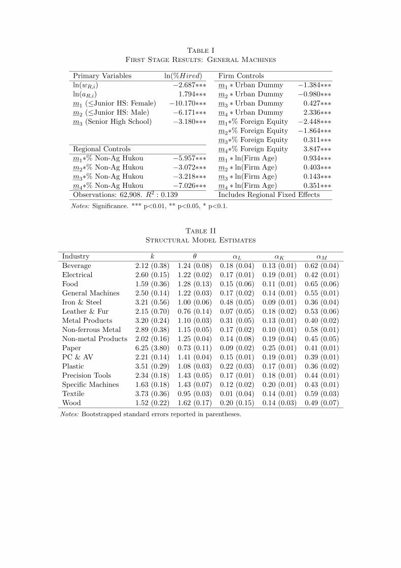
Table IFirst Stage Results: General Machines

Primary Variables ln(%Hired) Firm Controlsln(wR,i) −2.687∗∗∗ m1 ∗Urban Dummy −1.384∗∗∗ln(aR,i) 1.794∗∗∗ m2 ∗Urban Dummy −0.980∗∗∗m1 (≤Junior HS: Female) −10.170∗∗∗ m3 ∗Urban Dummy 0.427∗∗∗m2 (≤Junior HS: Male) −6.171∗∗∗ m4 ∗Urban Dummy 2.336∗∗∗m3 (Senior High School) −3.180∗∗∗ m1∗% Foreign Equity −2.448∗∗∗

m2∗% Foreign Equity −1.864∗∗∗m3∗% Foreign Equity 0.311∗∗∗

Regional Controls m4∗% Foreign Equity 3.847∗∗∗m1∗% Non-Ag Hukou −5.957∗∗∗ m1 ∗ ln(Firm Age) 0.934∗∗∗m2∗% Non-Ag Hukou −3.072∗∗∗ m2 ∗ ln(Firm Age) 0.403∗∗∗m3∗% Non-Ag Hukou −3.218∗∗∗ m3 ∗ ln(Firm Age) 0.143∗∗∗m4∗% Non-Ag Hukou −7.026∗∗∗ m4 ∗ ln(Firm Age) 0.351∗∗∗Observations: 62,908. R2 : 0.139 Includes Regional Fixed Effects

Notes: Significance. *** p<0.01, ** p<0.05, * p<0.1.

Table IIStructural Model Estimates

Industry k θ αL αK αMBeverage 2.12 (0.38) 1.24 (0.08) 0.18 (0.04) 0.13 (0.01) 0.62 (0.04)Electrical 2.60 (0.15) 1.22 (0.02) 0.17 (0.01) 0.19 (0.01) 0.42 (0.01)Food 1.59 (0.36) 1.28 (0.13) 0.15 (0.06) 0.11 (0.01) 0.65 (0.06)General Machines 2.50 (0.14) 1.22 (0.03) 0.17 (0.02) 0.14 (0.01) 0.55 (0.01)Iron & Steel 3.21 (0.56) 1.00 (0.06) 0.48 (0.05) 0.09 (0.01) 0.36 (0.04)Leather & Fur 2.15 (0.70) 0.76 (0.14) 0.07 (0.05) 0.18 (0.02) 0.53 (0.06)Metal Products 3.20 (0.24) 1.10 (0.03) 0.31 (0.05) 0.13 (0.01) 0.40 (0.02)Non-ferrous Metal 2.89 (0.38) 1.15 (0.05) 0.17 (0.02) 0.10 (0.01) 0.58 (0.01)Non-metal Products 2.02 (0.16) 1.25 (0.04) 0.14 (0.08) 0.19 (0.04) 0.45 (0.05)Paper 6.25 (3.80) 0.73 (0.11) 0.09 (0.02) 0.25 (0.01) 0.41 (0.01)PC & AV 2.21 (0.14) 1.41 (0.04) 0.15 (0.01) 0.19 (0.01) 0.39 (0.01)Plastic 3.51 (0.29) 1.08 (0.03) 0.22 (0.03) 0.17 (0.01) 0.36 (0.02)Precision Tools 2.34 (0.18) 1.43 (0.05) 0.17 (0.01) 0.18 (0.01) 0.44 (0.01)Specific Machines 1.63 (0.18) 1.43 (0.07) 0.12 (0.02) 0.20 (0.01) 0.43 (0.01)Textile 3.73 (0.36) 0.95 (0.03) 0.01 (0.04) 0.14 (0.01) 0.59 (0.03)Wood 1.52 (0.22) 1.62 (0.17) 0.20 (0.15) 0.14 (0.03) 0.49 (0.07)

Notes: Bootstrapped standard errors reported in parentheses.

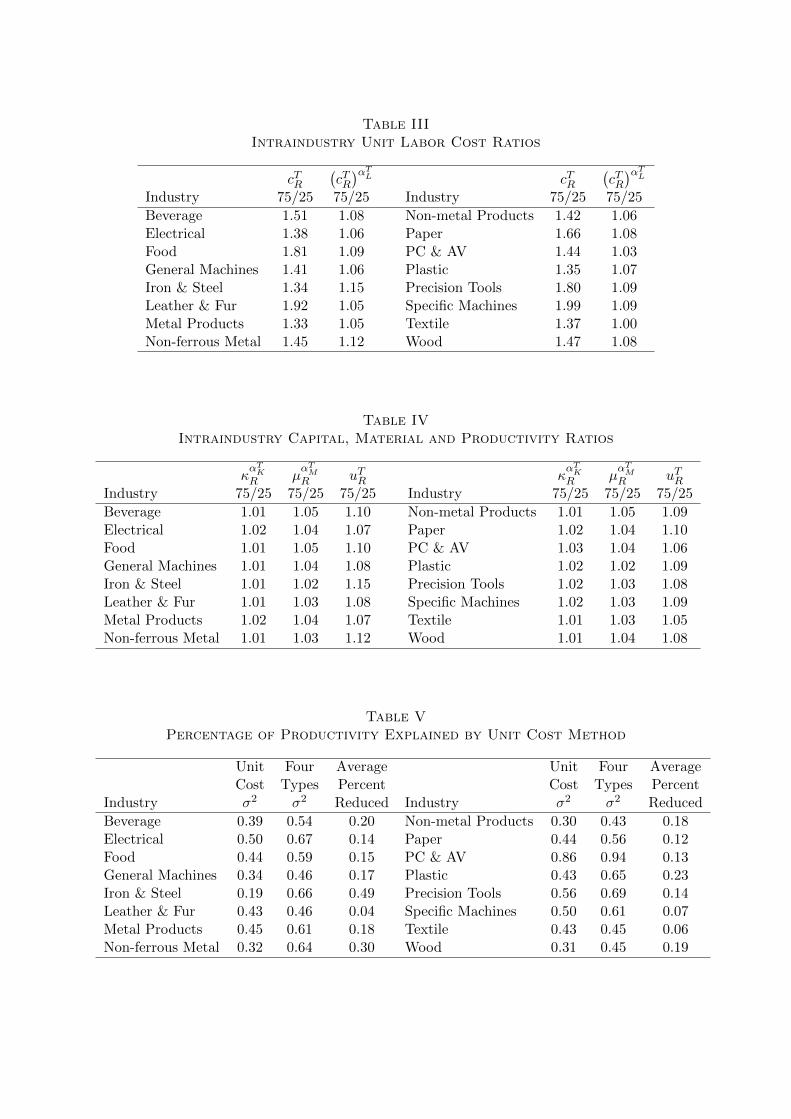
Table IIIIntraindustry Unit Labor Cost Ratios

cTR(cTR)αTL cTR

(cTR)αTL

Industry 75/25 75/25 Industry 75/25 75/25

Beverage 1.51 1.08 Non-metal Products 1.42 1.06Electrical 1.38 1.06 Paper 1.66 1.08Food 1.81 1.09 PC & AV 1.44 1.03General Machines 1.41 1.06 Plastic 1.35 1.07Iron & Steel 1.34 1.15 Precision Tools 1.80 1.09Leather & Fur 1.92 1.05 Specific Machines 1.99 1.09Metal Products 1.33 1.05 Textile 1.37 1.00Non-ferrous Metal 1.45 1.12 Wood 1.47 1.08

Table IVIntraindustry Capital, Material and Productivity Ratios

καTKR µ

αTMR uTR κ

αTKR µ

αTMR uTR

Industry 75/25 75/25 75/25 Industry 75/25 75/25 75/25

Beverage 1.01 1.05 1.10 Non-metal Products 1.01 1.05 1.09Electrical 1.02 1.04 1.07 Paper 1.02 1.04 1.10Food 1.01 1.05 1.10 PC & AV 1.03 1.04 1.06General Machines 1.01 1.04 1.08 Plastic 1.02 1.02 1.09Iron & Steel 1.01 1.02 1.15 Precision Tools 1.02 1.03 1.08Leather & Fur 1.01 1.03 1.08 Specific Machines 1.02 1.03 1.09Metal Products 1.02 1.04 1.07 Textile 1.01 1.03 1.05Non-ferrous Metal 1.01 1.03 1.12 Wood 1.01 1.04 1.08

Table VPercentage of Productivity Explained by Unit Cost Method

Unit Four Average Unit Four AverageCost Types Percent Cost Types Percent

Industry σ2 σ2 Reduced Industry σ2 σ2 Reduced

Beverage 0.39 0.54 0.20 Non-metal Products 0.30 0.43 0.18Electrical 0.50 0.67 0.14 Paper 0.44 0.56 0.12Food 0.44 0.59 0.15 PC & AV 0.86 0.94 0.13General Machines 0.34 0.46 0.17 Plastic 0.43 0.65 0.23Iron & Steel 0.19 0.66 0.49 Precision Tools 0.56 0.69 0.14Leather & Fur 0.43 0.46 0.04 Specific Machines 0.50 0.61 0.07Metal Products 0.45 0.61 0.18 Textile 0.43 0.45 0.06Non-ferrous Metal 0.32 0.64 0.30 Wood 0.31 0.45 0.19

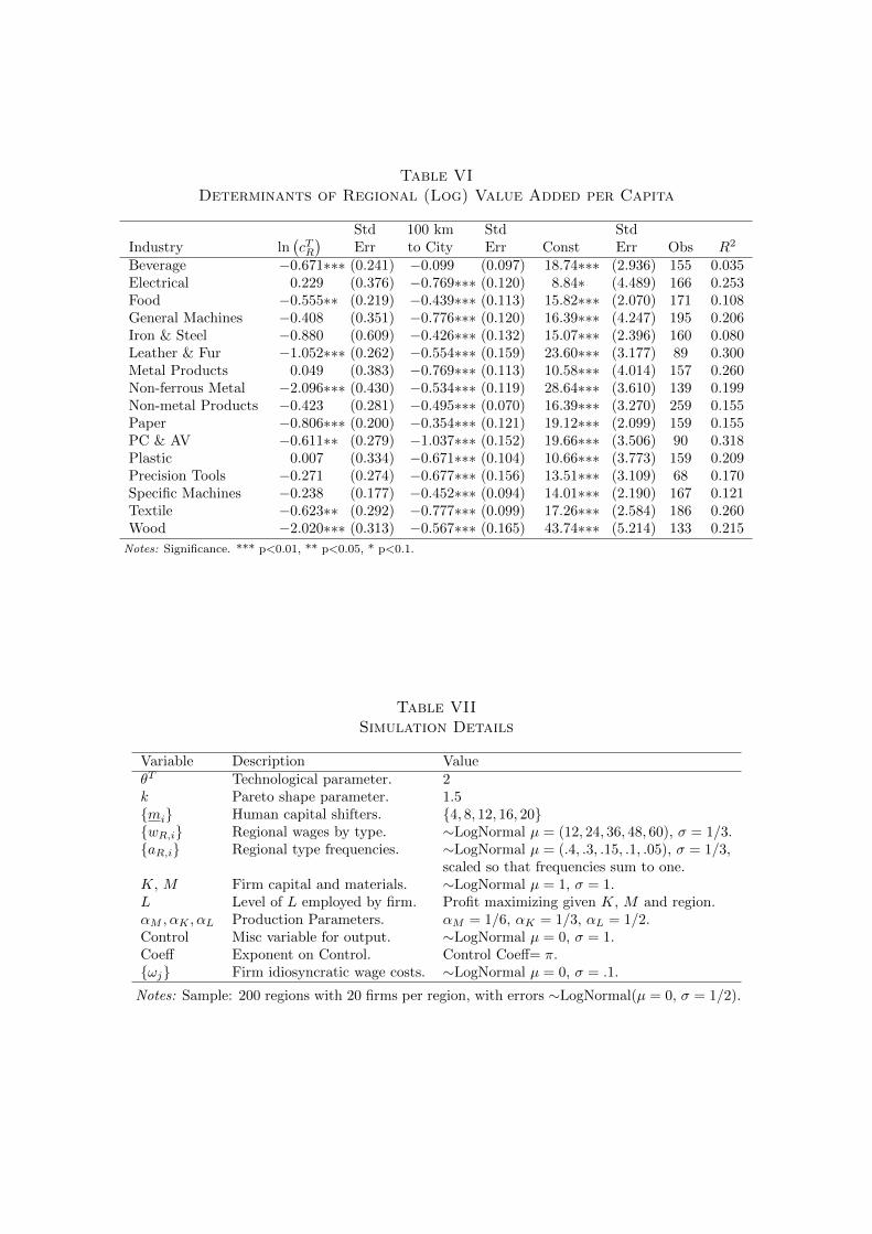
Table VIDeterminants of Regional (Log) Value Added per Capita

Std 100 km Std StdIndustry ln

(cTR)

Err to City Err Const Err Obs R2

Beverage −0.671∗∗∗ (0.241) −0.099 (0.097) 18.74∗∗∗ (2.936) 155 0.035Electrical 0.229 (0.376) −0.769∗∗∗ (0.120) 8.84∗ (4.489) 166 0.253Food −0.555∗∗ (0.219) −0.439∗∗∗ (0.113) 15.82∗∗∗ (2.070) 171 0.108General Machines −0.408 (0.351) −0.776∗∗∗ (0.120) 16.39∗∗∗ (4.247) 195 0.206Iron & Steel −0.880 (0.609) −0.426∗∗∗ (0.132) 15.07∗∗∗ (2.396) 160 0.080Leather & Fur −1.052∗∗∗ (0.262) −0.554∗∗∗ (0.159) 23.60∗∗∗ (3.177) 89 0.300Metal Products 0.049 (0.383) −0.769∗∗∗ (0.113) 10.58∗∗∗ (4.014) 157 0.260Non-ferrous Metal −2.096∗∗∗ (0.430) −0.534∗∗∗ (0.119) 28.64∗∗∗ (3.610) 139 0.199Non-metal Products −0.423 (0.281) −0.495∗∗∗ (0.070) 16.39∗∗∗ (3.270) 259 0.155Paper −0.806∗∗∗ (0.200) −0.354∗∗∗ (0.121) 19.12∗∗∗ (2.099) 159 0.155PC & AV −0.611∗∗ (0.279) −1.037∗∗∗ (0.152) 19.66∗∗∗ (3.506) 90 0.318Plastic 0.007 (0.334) −0.671∗∗∗ (0.104) 10.66∗∗∗ (3.773) 159 0.209Precision Tools −0.271 (0.274) −0.677∗∗∗ (0.156) 13.51∗∗∗ (3.109) 68 0.170Specific Machines −0.238 (0.177) −0.452∗∗∗ (0.094) 14.01∗∗∗ (2.190) 167 0.121Textile −0.623∗∗ (0.292) −0.777∗∗∗ (0.099) 17.26∗∗∗ (2.584) 186 0.260Wood −2.020∗∗∗ (0.313) −0.567∗∗∗ (0.165) 43.74∗∗∗ (5.214) 133 0.215

Notes: Significance. *** p<0.01, ** p<0.05, * p<0.1.

Table VIISimulation Details

Variable Description ValueθT Technological parameter. 2k Pareto shape parameter. 1.5{mi} Human capital shifters. {4, 8, 12, 16, 20}{wR,i} Regional wages by type. ∼LogNormal µ = (12, 24, 36, 48, 60), σ = 1/3.{aR,i} Regional type frequencies. ∼LogNormal µ = (.4, .3, .15, .1, .05), σ = 1/3,

scaled so that frequencies sum to one.K, M Firm capital and materials. ∼LogNormal µ = 1, σ = 1.L Level of L employed by firm. Profit maximizing given K, M and region.αM , αK , αL Production Parameters. αM = 1/6, αK = 1/3, αL = 1/2.Control Misc variable for output. ∼LogNormal µ = 0, σ = 1.Coeff Exponent on Control. Control Coeff= π.{ωj} Firm idiosyncratic wage costs. ∼LogNormal µ = 0, σ = .1.

Notes: Sample: 200 regions with 20 firms per region, with errors ∼LogNormal(µ = 0, σ = 1/2).

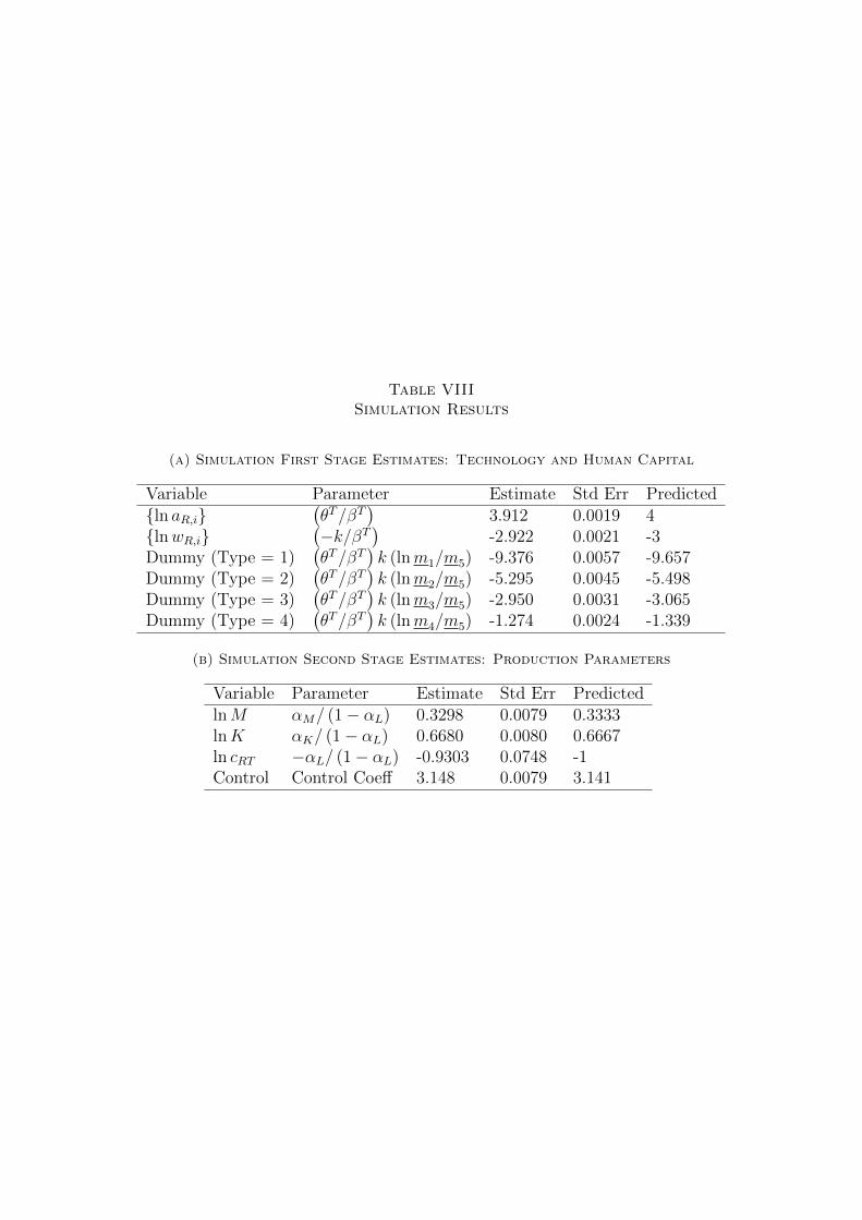
Table VIIISimulation Results

(a) Simulation First Stage Estimates: Technology and Human Capital

Variable Parameter Estimate Std Err Predicted{ln aR,i}

(θT/βT

)3.912 0.0019 4

{lnwR,i}(−k/βT

)-2.922 0.0021 -3

Dummy (Type = 1)(θT/βT

)k (lnm1/m5) -9.376 0.0057 -9.657

Dummy (Type = 2)(θT/βT

)k (lnm2/m5) -5.295 0.0045 -5.498

Dummy (Type = 3)(θT/βT

)k (lnm3/m5) -2.950 0.0031 -3.065

Dummy (Type = 4)(θT/βT

)k (lnm4/m5) -1.274 0.0024 -1.339

(b) Simulation Second Stage Estimates: Production Parameters

Variable Parameter Estimate Std Err PredictedlnM αM/ (1− αL) 0.3298 0.0079 0.3333lnK αK/ (1− αL) 0.6680 0.0080 0.6667ln cRT −αL/ (1− αL) -0.9303 0.0748 -1Control Control Coeff 3.148 0.0079 3.141

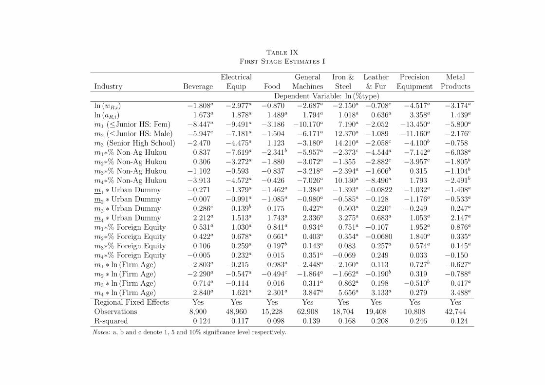
Table IXFirst Stage Estimates I

Electrical General Iron & Leather Precision MetalIndustry Beverage Equip Food Machines Steel & Fur Equipment Products

Dependent Variable: ln (%type)ln (wR,i) −1.808a −2.977a −0.870 −2.687a −2.150a −0.708c −4.517a −3.174a

ln (aR,i) 1.673a 1.878a 1.489a 1.794a 1.018a 0.636a 3.358a 1.439a

m1 (≤Junior HS: Fem) −8.447a −9.491a −3.186 −10.170a 7.190a −2.052 −13.450a −5.800a

m2 (≤Junior HS: Male) −5.947c −7.181a −1.504 −6.171a 12.370a −1.089 −11.160a −2.176c

m3 (Senior High School) −2.470 −4.475a 1.123 −3.180a 14.210a −2.058c −4.100b −0.758m1∗% Non-Ag Hukou 0.837 −7.619a −2.341b −5.957a −2.373c −4.544a −7.142a −6.038a

m2∗% Non-Ag Hukou 0.306 −3.272a −1.880 −3.072a −1.355 −2.882c −3.957c −1.805b

m3∗% Non-Ag Hukou −1.102 −0.593 −0.837 −3.218a −2.394a −1.606b 0.315 −1.104b

m4∗% Non-Ag Hukou −3.913 −4.572a −0.426 −7.026a 10.130a −8.496a 1.793 −2.491b

m1 ∗ Urban Dummy −0.271 −1.379a −1.462a −1.384a −1.393a −0.0822 −1.032a −1.408a

m2 ∗ Urban Dummy −0.007 −0.991a −1.085a −0.980a −0.585a −0.128 −1.176a −0.533a

m3 ∗ Urban Dummy 0.286c 0.139b 0.175 0.427a 0.503a 0.220c −0.249 0.247a

m4 ∗ Urban Dummy 2.212a 1.513a 1.743a 2.336a 3.275a 0.683a 1.053a 2.147a

m1∗% Foreign Equity 0.531a 1.030a 0.841a 0.934a 0.751a −0.107 1.952a 0.876a

m2∗% Foreign Equity 0.422a 0.678a 0.661a 0.403a 0.354a −0.0680 1.840a 0.335a

m3∗% Foreign Equity 0.106 0.259a 0.197b 0.143a 0.083 0.257a 0.574a 0.145a

m4∗% Foreign Equity −0.005 0.232a 0.015 0.351a −0.069 0.249 0.033 −0.150m1 ∗ ln (Firm Age) −2.803a −0.215 −0.983a −2.448a −2.160a 0.113 0.727b −0.627a

m2 ∗ ln (Firm Age) −2.290a −0.547a −0.494c −1.864a −1.662a −0.190b 0.319 −0.788a

m3 ∗ ln (Firm Age) 0.714a −0.114 0.016 0.311a 0.862a 0.198 −0.510b 0.417a

m4 ∗ ln (Firm Age) 2.840a 1.621a 2.301a 3.847a 5.656a 3.133a 0.279 3.488a

Regional Fixed Effects Yes Yes Yes Yes Yes Yes Yes YesObservations 8,900 48,960 15,228 62,908 18,704 19,408 10,808 42,744R-squared 0.124 0.117 0.098 0.139 0.168 0.208 0.246 0.124

Notes: a, b and c denote 1, 5 and 10% significance level respectively.

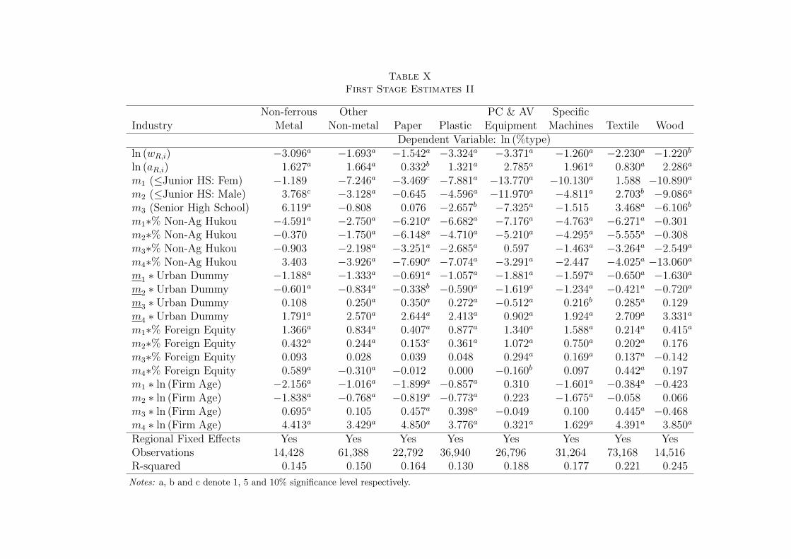
Table XFirst Stage Estimates II

Non-ferrous Other PC & AV SpecificIndustry Metal Non-metal Paper Plastic Equipment Machines Textile Wood

Dependent Variable: ln (%type)ln (wR,i) −3.096a −1.693a −1.542a −3.324a −3.371a −1.260a −2.230a −1.220b

ln (aR,i) 1.627a 1.664a 0.332b 1.321a 2.785a 1.961a 0.830a 2.286a

m1 (≤Junior HS: Fem) −1.189 −7.246a −3.469c −7.881a −13.770a −10.130a 1.588 −10.890a

m2 (≤Junior HS: Male) 3.768c −3.128a −0.645 −4.596a −11.970a −4.811a 2.703b −9.086a

m3 (Senior High School) 6.119a −0.808 0.076 −2.657b −7.325a −1.515 3.468a −6.106b

m1∗% Non-Ag Hukou −4.591a −2.750a −6.210a −6.682a −7.176a −4.763a −6.271a −0.301m2∗% Non-Ag Hukou −0.370 −1.750a −6.148a −4.710a −5.210a −4.295a −5.555a −0.308m3∗% Non-Ag Hukou −0.903 −2.198a −3.251a −2.685a 0.597 −1.463a −3.264a −2.549a

m4∗% Non-Ag Hukou 3.403 −3.926a −7.690a −7.074a −3.291a −2.447 −4.025a −13.060a

m1 ∗ Urban Dummy −1.188a −1.333a −0.691a −1.057a −1.881a −1.597a −0.650a −1.630a

m2 ∗ Urban Dummy −0.601a −0.834a −0.338b −0.590a −1.619a −1.234a −0.421a −0.720a

m3 ∗ Urban Dummy 0.108 0.250a 0.350a 0.272a −0.512a 0.216b 0.285a 0.129m4 ∗ Urban Dummy 1.791a 2.570a 2.644a 2.413a 0.902a 1.924a 2.709a 3.331a

m1∗% Foreign Equity 1.366a 0.834a 0.407a 0.877a 1.340a 1.588a 0.214a 0.415a

m2∗% Foreign Equity 0.432a 0.244a 0.153c 0.361a 1.072a 0.750a 0.202a 0.176m3∗% Foreign Equity 0.093 0.028 0.039 0.048 0.294a 0.169a 0.137a −0.142m4∗% Foreign Equity 0.589a −0.310a −0.012 0.000 −0.160b 0.097 0.442a 0.197m1 ∗ ln (Firm Age) −2.156a −1.016a −1.899a −0.857a 0.310 −1.601a −0.384a −0.423m2 ∗ ln (Firm Age) −1.838a −0.768a −0.819a −0.773a 0.223 −1.675a −0.058 0.066m3 ∗ ln (Firm Age) 0.695a 0.105 0.457a 0.398a −0.049 0.100 0.445a −0.468m4 ∗ ln (Firm Age) 4.413a 3.429a 4.850a 3.776a 0.321a 1.629a 4.391a 3.850a

Regional Fixed Effects Yes Yes Yes Yes Yes Yes Yes YesObservations 14,428 61,388 22,792 36,940 26,796 31,264 73,168 14,516R-squared 0.145 0.150 0.164 0.130 0.188 0.177 0.221 0.245

Notes: a, b and c denote 1, 5 and 10% significance level respectively.

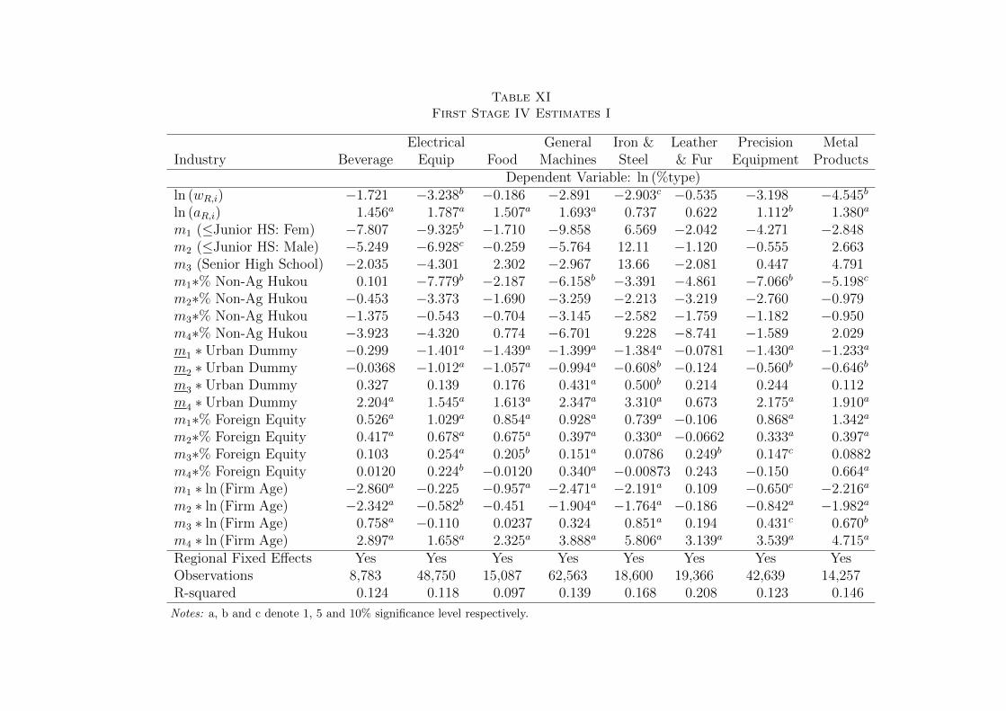
Table XIFirst Stage IV Estimates I

Electrical General Iron & Leather Precision MetalIndustry Beverage Equip Food Machines Steel & Fur Equipment Products

Dependent Variable: ln (%type)ln (wR,i) −1.721 −3.238b −0.186 −2.891 −2.903c −0.535 −3.198 −4.545b

ln (aR,i) 1.456a 1.787a 1.507a 1.693a 0.737 0.622 1.112b 1.380a

m1 (≤Junior HS: Fem) −7.807 −9.325b −1.710 −9.858 6.569 −2.042 −4.271 −2.848m2 (≤Junior HS: Male) −5.249 −6.928c −0.259 −5.764 12.11 −1.120 −0.555 2.663m3 (Senior High School) −2.035 −4.301 2.302 −2.967 13.66 −2.081 0.447 4.791m1∗% Non-Ag Hukou 0.101 −7.779b −2.187 −6.158b −3.391 −4.861 −7.066b −5.198c

m2∗% Non-Ag Hukou −0.453 −3.373 −1.690 −3.259 −2.213 −3.219 −2.760 −0.979m3∗% Non-Ag Hukou −1.375 −0.543 −0.704 −3.145 −2.582 −1.759 −1.182 −0.950m4∗% Non-Ag Hukou −3.923 −4.320 0.774 −6.701 9.228 −8.741 −1.589 2.029m1 ∗ Urban Dummy −0.299 −1.401a −1.439a −1.399a −1.384a −0.0781 −1.430a −1.233a

m2 ∗ Urban Dummy −0.0368 −1.012a −1.057a −0.994a −0.608b −0.124 −0.560b −0.646b

m3 ∗ Urban Dummy 0.327 0.139 0.176 0.431a 0.500b 0.214 0.244 0.112m4 ∗ Urban Dummy 2.204a 1.545a 1.613a 2.347a 3.310a 0.673 2.175a 1.910a

m1∗% Foreign Equity 0.526a 1.029a 0.854a 0.928a 0.739a −0.106 0.868a 1.342a

m2∗% Foreign Equity 0.417a 0.678a 0.675a 0.397a 0.330a −0.0662 0.333a 0.397a

m3∗% Foreign Equity 0.103 0.254a 0.205b 0.151a 0.0786 0.249b 0.147c 0.0882m4∗% Foreign Equity 0.0120 0.224b −0.0120 0.340a −0.00873 0.243 −0.150 0.664a

m1 ∗ ln (Firm Age) −2.860a −0.225 −0.957a −2.471a −2.191a 0.109 −0.650c −2.216a

m2 ∗ ln (Firm Age) −2.342a −0.582b −0.451 −1.904a −1.764a −0.186 −0.842a −1.982a

m3 ∗ ln (Firm Age) 0.758a −0.110 0.0237 0.324 0.851a 0.194 0.431c 0.670b

m4 ∗ ln (Firm Age) 2.897a 1.658a 2.325a 3.888a 5.806a 3.139a 3.539a 4.715a

Regional Fixed Effects Yes Yes Yes Yes Yes Yes Yes YesObservations 8,783 48,750 15,087 62,563 18,600 19,366 42,639 14,257R-squared 0.124 0.118 0.097 0.139 0.168 0.208 0.123 0.146

Notes: a, b and c denote 1, 5 and 10% significance level respectively.

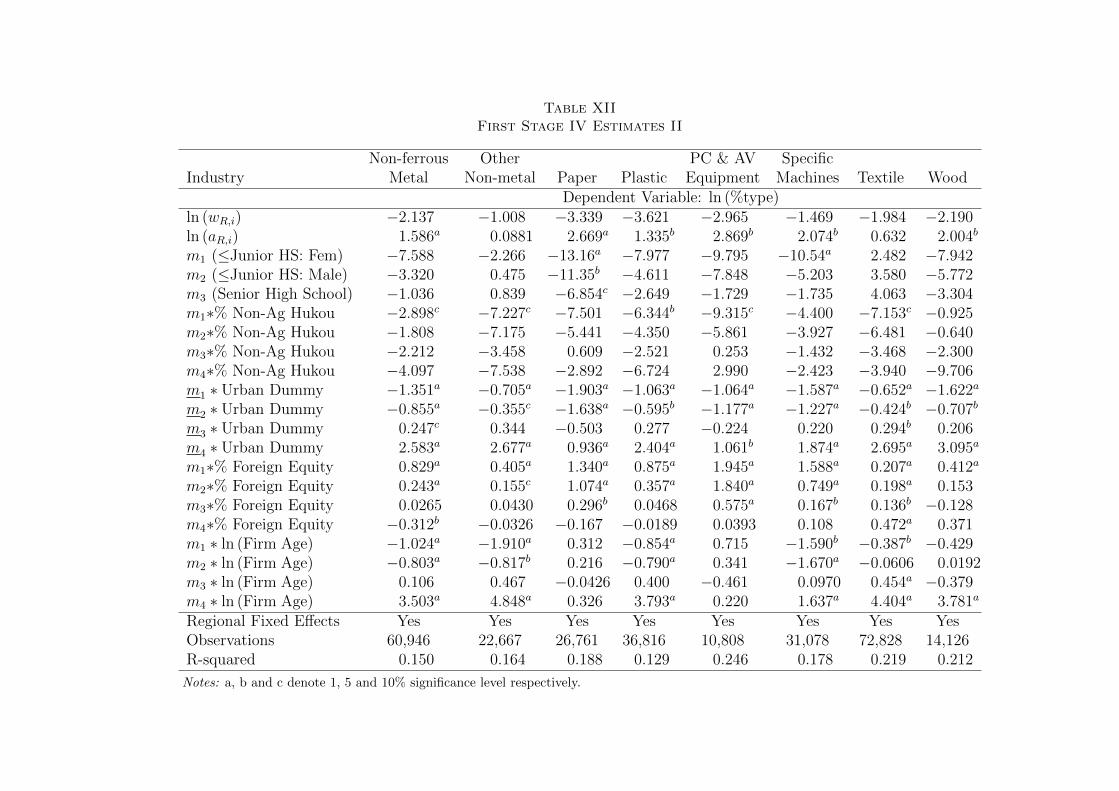
Table XIIFirst Stage IV Estimates II

Non-ferrous Other PC & AV SpecificIndustry Metal Non-metal Paper Plastic Equipment Machines Textile Wood

Dependent Variable: ln (%type)ln (wR,i) −2.137 −1.008 −3.339 −3.621 −2.965 −1.469 −1.984 −2.190ln (aR,i) 1.586a 0.0881 2.669a 1.335b 2.869b 2.074b 0.632 2.004b

m1 (≤Junior HS: Fem) −7.588 −2.266 −13.16a −7.977 −9.795 −10.54a 2.482 −7.942m2 (≤Junior HS: Male) −3.320 0.475 −11.35b −4.611 −7.848 −5.203 3.580 −5.772m3 (Senior High School) −1.036 0.839 −6.854c −2.649 −1.729 −1.735 4.063 −3.304m1∗% Non-Ag Hukou −2.898c −7.227c −7.501 −6.344b −9.315c −4.400 −7.153c −0.925m2∗% Non-Ag Hukou −1.808 −7.175 −5.441 −4.350 −5.861 −3.927 −6.481 −0.640m3∗% Non-Ag Hukou −2.212 −3.458 0.609 −2.521 0.253 −1.432 −3.468 −2.300m4∗% Non-Ag Hukou −4.097 −7.538 −2.892 −6.724 2.990 −2.423 −3.940 −9.706m1 ∗ Urban Dummy −1.351a −0.705a −1.903a −1.063a −1.064a −1.587a −0.652a −1.622a

m2 ∗ Urban Dummy −0.855a −0.355c −1.638a −0.595b −1.177a −1.227a −0.424b −0.707b

m3 ∗ Urban Dummy 0.247c 0.344 −0.503 0.277 −0.224 0.220 0.294b 0.206m4 ∗ Urban Dummy 2.583a 2.677a 0.936a 2.404a 1.061b 1.874a 2.695a 3.095a

m1∗% Foreign Equity 0.829a 0.405a 1.340a 0.875a 1.945a 1.588a 0.207a 0.412a

m2∗% Foreign Equity 0.243a 0.155c 1.074a 0.357a 1.840a 0.749a 0.198a 0.153m3∗% Foreign Equity 0.0265 0.0430 0.296b 0.0468 0.575a 0.167b 0.136b −0.128m4∗% Foreign Equity −0.312b −0.0326 −0.167 −0.0189 0.0393 0.108 0.472a 0.371m1 ∗ ln (Firm Age) −1.024a −1.910a 0.312 −0.854a 0.715 −1.590b −0.387b −0.429m2 ∗ ln (Firm Age) −0.803a −0.817b 0.216 −0.790a 0.341 −1.670a −0.0606 0.0192m3 ∗ ln (Firm Age) 0.106 0.467 −0.0426 0.400 −0.461 0.0970 0.454a −0.379m4 ∗ ln (Firm Age) 3.503a 4.848a 0.326 3.793a 0.220 1.637a 4.404a 3.781a

Regional Fixed Effects Yes Yes Yes Yes Yes Yes Yes YesObservations 60,946 22,667 26,761 36,816 10,808 31,078 72,828 14,126R-squared 0.150 0.164 0.188 0.129 0.246 0.178 0.219 0.212

Notes: a, b and c denote 1, 5 and 10% significance level respectively.

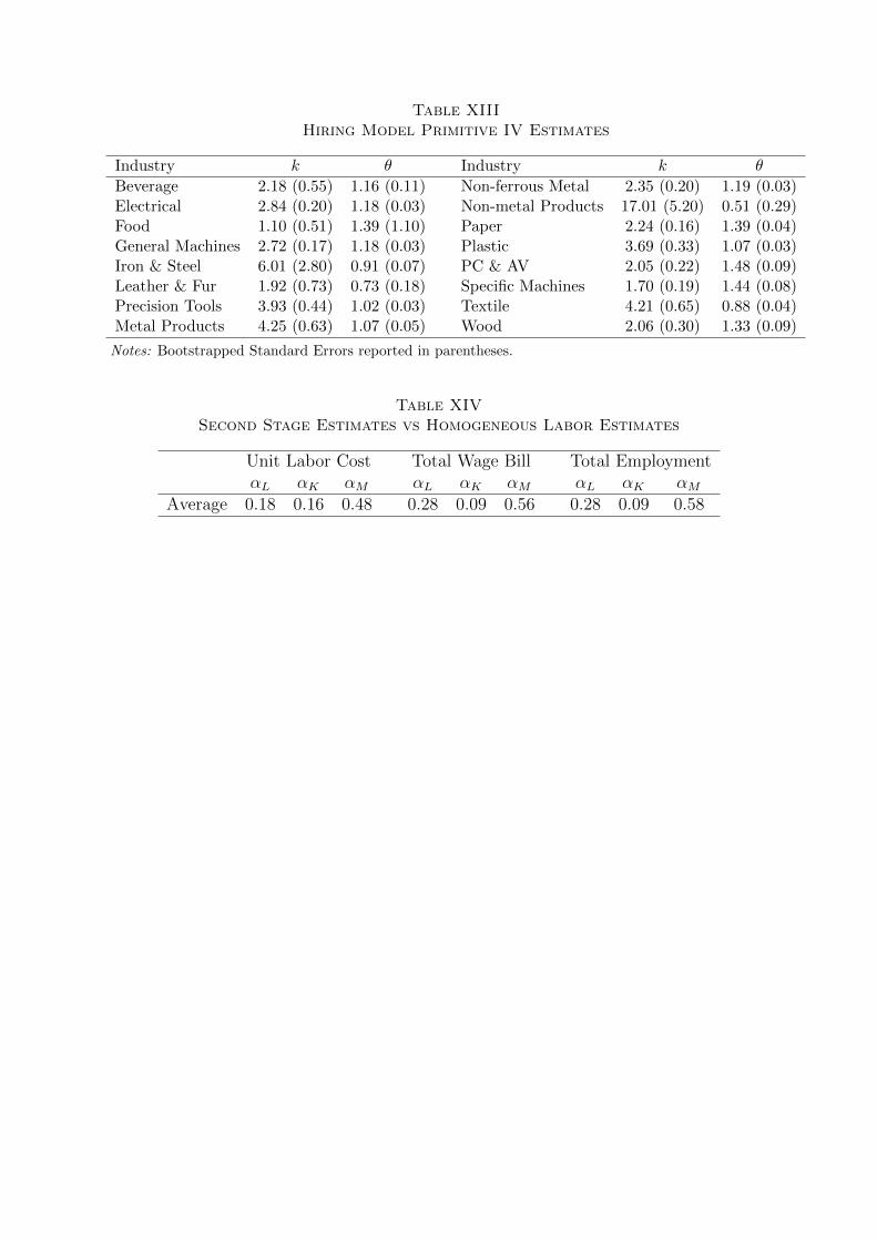
Table XIIIHiring Model Primitive IV Estimates

Industry k θ Industry k θ

Beverage 2.18 (0.55) 1.16 (0.11) Non-ferrous Metal 2.35 (0.20) 1.19 (0.03)Electrical 2.84 (0.20) 1.18 (0.03) Non-metal Products 17.01 (5.20) 0.51 (0.29)Food 1.10 (0.51) 1.39 (1.10) Paper 2.24 (0.16) 1.39 (0.04)General Machines 2.72 (0.17) 1.18 (0.03) Plastic 3.69 (0.33) 1.07 (0.03)Iron & Steel 6.01 (2.80) 0.91 (0.07) PC & AV 2.05 (0.22) 1.48 (0.09)Leather & Fur 1.92 (0.73) 0.73 (0.18) Specific Machines 1.70 (0.19) 1.44 (0.08)Precision Tools 3.93 (0.44) 1.02 (0.03) Textile 4.21 (0.65) 0.88 (0.04)Metal Products 4.25 (0.63) 1.07 (0.05) Wood 2.06 (0.30) 1.33 (0.09)

Notes: Bootstrapped Standard Errors reported in parentheses.

Table XIVSecond Stage Estimates vs Homogeneous Labor Estimates

Unit Labor Cost Total Wage Bill Total EmploymentαL αK αM αL αK αM αL αK αM

Average 0.18 0.16 0.48 0.28 0.09 0.56 0.28 0.09 0.58

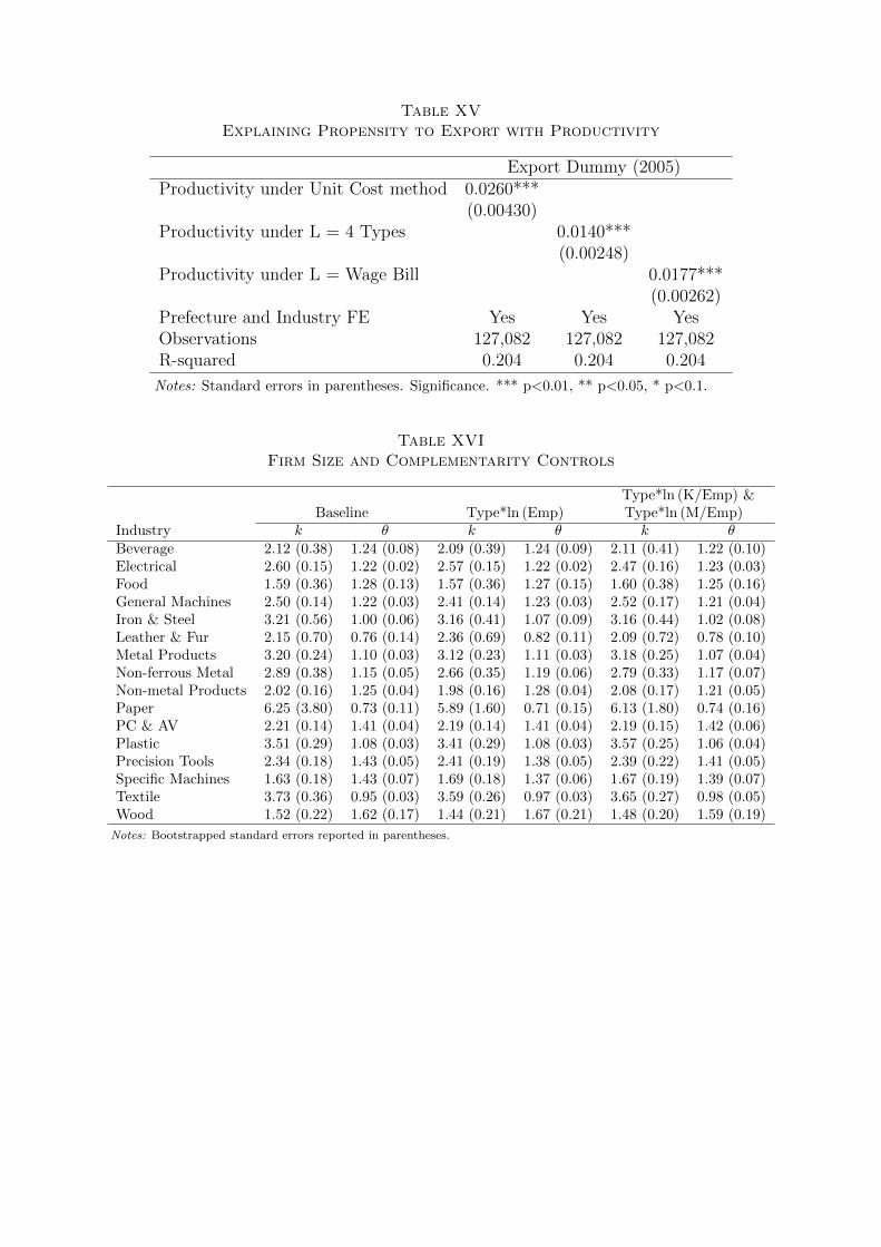
Table XVExplaining Propensity to Export with Productivity

Export Dummy (2005)Productivity under Unit Cost method 0.0260***

(0.00430)Productivity under L = 4 Types 0.0140***

(0.00248)Productivity under L = Wage Bill 0.0177***

(0.00262)Prefecture and Industry FE Yes Yes YesObservations 127,082 127,082 127,082R-squared 0.204 0.204 0.204

Notes: Standard errors in parentheses. Significance. *** p<0.01, ** p<0.05, * p<0.1.

Table XVIFirm Size and Complementarity Controls

Type*ln (K/Emp) &Baseline Type*ln (Emp) Type*ln (M/Emp)

Industry k θ k θ k θBeverage 2.12 (0.38) 1.24 (0.08) 2.09 (0.39) 1.24 (0.09) 2.11 (0.41) 1.22 (0.10)Electrical 2.60 (0.15) 1.22 (0.02) 2.57 (0.15) 1.22 (0.02) 2.47 (0.16) 1.23 (0.03)Food 1.59 (0.36) 1.28 (0.13) 1.57 (0.36) 1.27 (0.15) 1.60 (0.38) 1.25 (0.16)General Machines 2.50 (0.14) 1.22 (0.03) 2.41 (0.14) 1.23 (0.03) 2.52 (0.17) 1.21 (0.04)Iron & Steel 3.21 (0.56) 1.00 (0.06) 3.16 (0.41) 1.07 (0.09) 3.16 (0.44) 1.02 (0.08)Leather & Fur 2.15 (0.70) 0.76 (0.14) 2.36 (0.69) 0.82 (0.11) 2.09 (0.72) 0.78 (0.10)Metal Products 3.20 (0.24) 1.10 (0.03) 3.12 (0.23) 1.11 (0.03) 3.18 (0.25) 1.07 (0.04)Non-ferrous Metal 2.89 (0.38) 1.15 (0.05) 2.66 (0.35) 1.19 (0.06) 2.79 (0.33) 1.17 (0.07)Non-metal Products 2.02 (0.16) 1.25 (0.04) 1.98 (0.16) 1.28 (0.04) 2.08 (0.17) 1.21 (0.05)Paper 6.25 (3.80) 0.73 (0.11) 5.89 (1.60) 0.71 (0.15) 6.13 (1.80) 0.74 (0.16)PC & AV 2.21 (0.14) 1.41 (0.04) 2.19 (0.14) 1.41 (0.04) 2.19 (0.15) 1.42 (0.06)Plastic 3.51 (0.29) 1.08 (0.03) 3.41 (0.29) 1.08 (0.03) 3.57 (0.25) 1.06 (0.04)Precision Tools 2.34 (0.18) 1.43 (0.05) 2.41 (0.19) 1.38 (0.05) 2.39 (0.22) 1.41 (0.05)Specific Machines 1.63 (0.18) 1.43 (0.07) 1.69 (0.18) 1.37 (0.06) 1.67 (0.19) 1.39 (0.07)Textile 3.73 (0.36) 0.95 (0.03) 3.59 (0.26) 0.97 (0.03) 3.65 (0.27) 0.98 (0.05)Wood 1.52 (0.22) 1.62 (0.17) 1.44 (0.21) 1.67 (0.21) 1.48 (0.20) 1.59 (0.19)

Notes: Bootstrapped standard errors reported in parentheses.

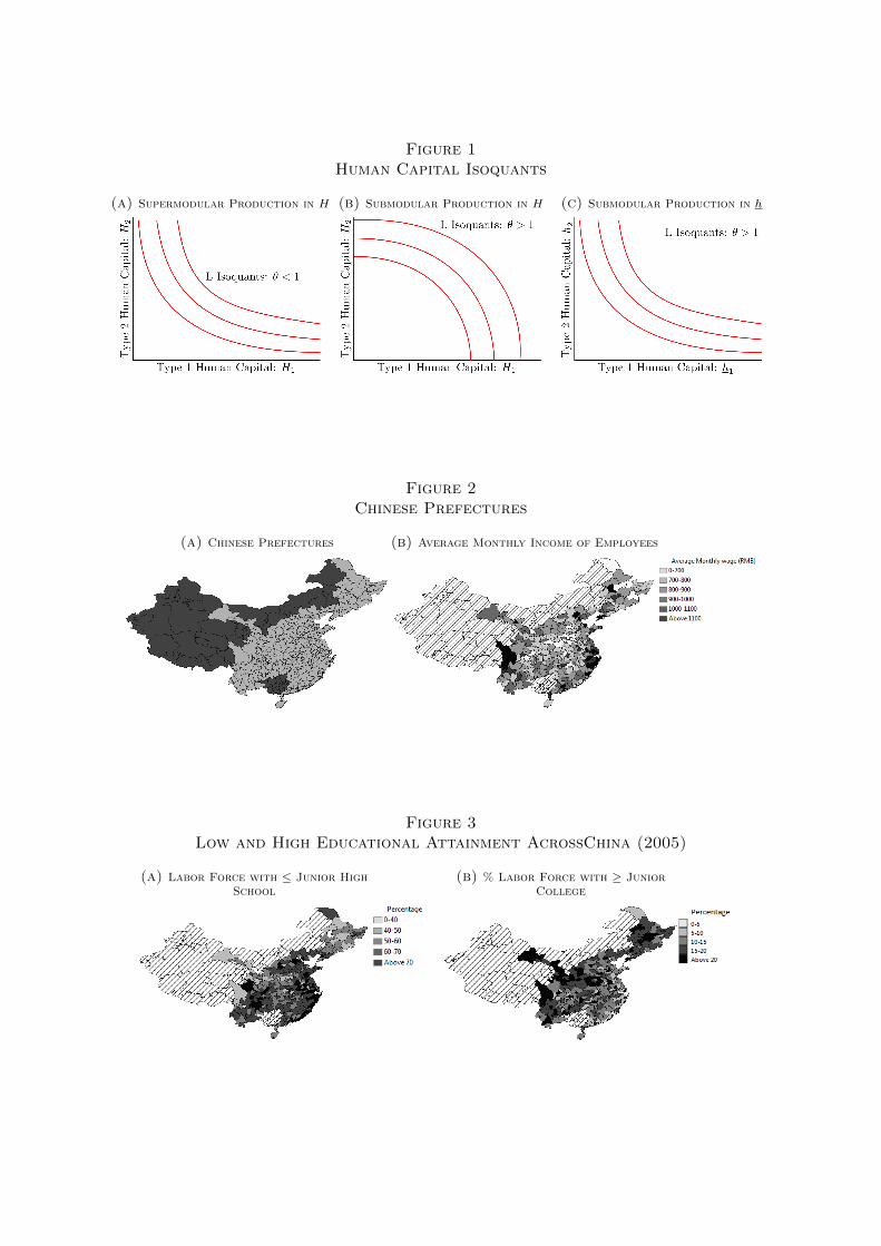
Figure 1Human Capital Isoquants

(a) Supermodular Production in H (b) Submodular Production in H (c) Submodular Production in h

Figure 2Chinese Prefectures

(a) Chinese Prefectures (b) Average Monthly Income of Employees

Figure 3Low and High Educational Attainment AcrossChina (2005)

(a) Labor Force with ≤ Junior HighSchool

(b) % Labor Force with ≥ JuniorCollege

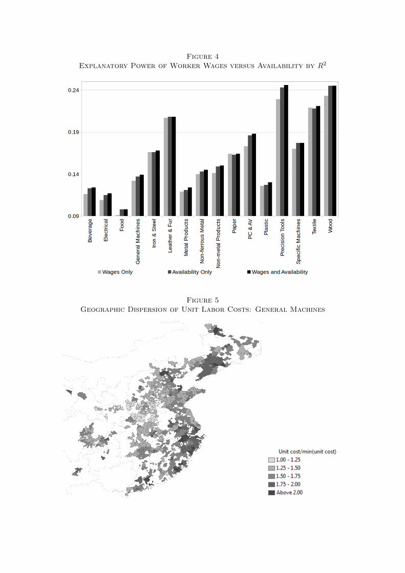
Figure 4Explanatory Power of Worker Wages versus Availability by R2

Figure 5Geographic Dispersion of Unit Labor Costs: General Machines

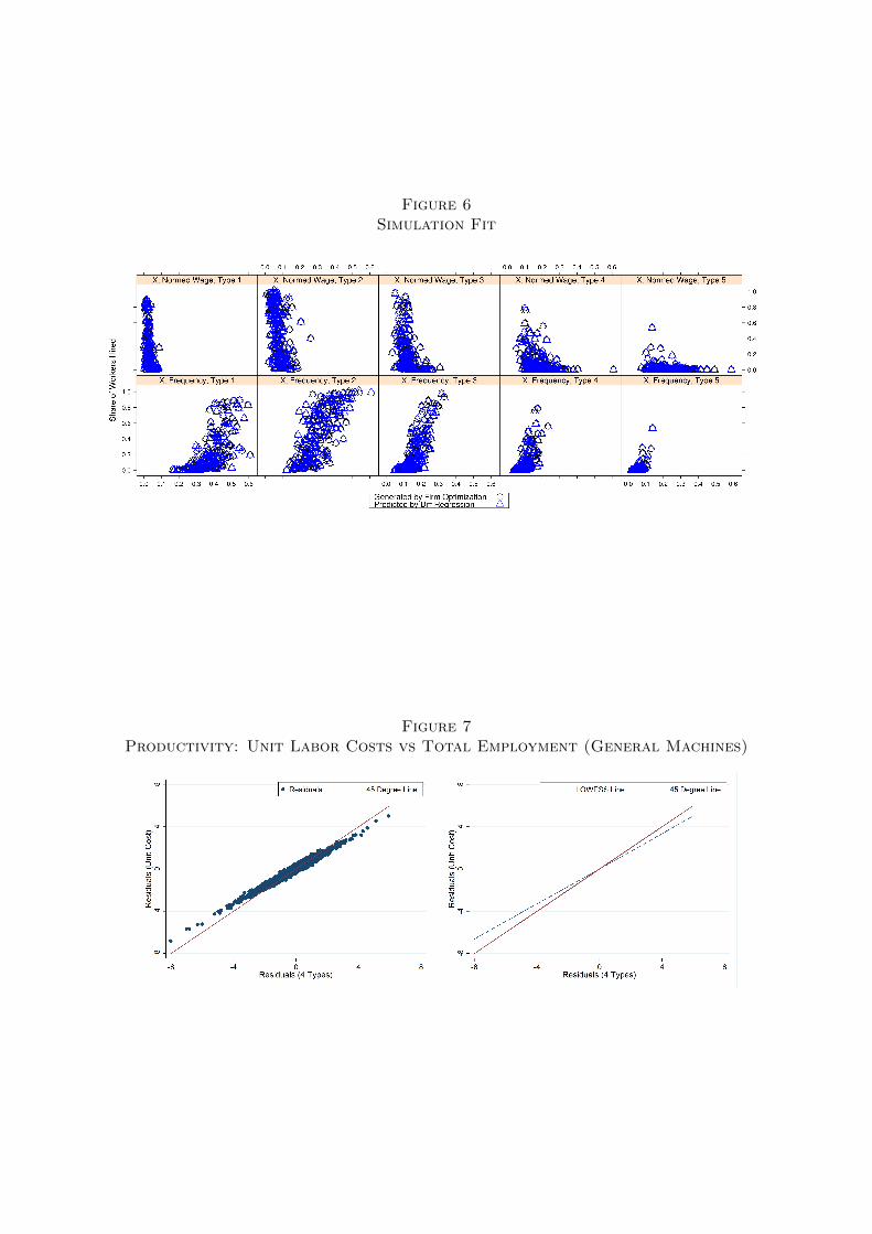
Figure 6Simulation Fit

Figure 7Productivity: Unit Labor Costs vs Total Employment (General Machines)

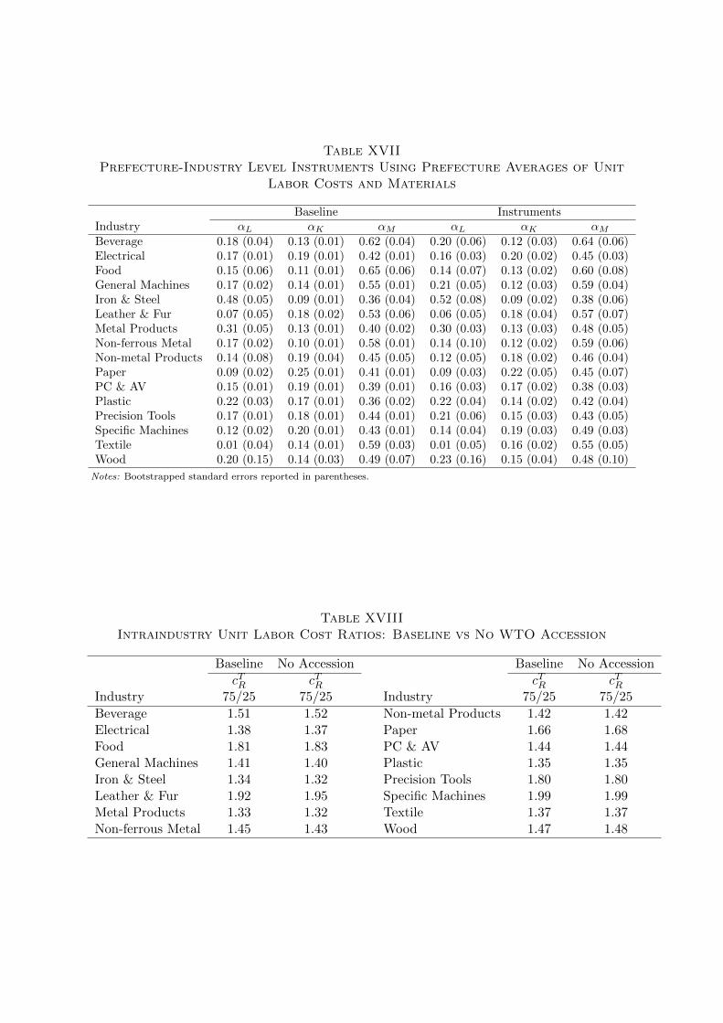
Table XVIIPrefecture-Industry Level Instruments Using Prefecture Averages of Unit

Labor Costs and Materials

Baseline InstrumentsIndustry αL αK αM αL αK αMBeverage 0.18 (0.04) 0.13 (0.01) 0.62 (0.04) 0.20 (0.06) 0.12 (0.03) 0.64 (0.06)Electrical 0.17 (0.01) 0.19 (0.01) 0.42 (0.01) 0.16 (0.03) 0.20 (0.02) 0.45 (0.03)Food 0.15 (0.06) 0.11 (0.01) 0.65 (0.06) 0.14 (0.07) 0.13 (0.02) 0.60 (0.08)General Machines 0.17 (0.02) 0.14 (0.01) 0.55 (0.01) 0.21 (0.05) 0.12 (0.03) 0.59 (0.04)Iron & Steel 0.48 (0.05) 0.09 (0.01) 0.36 (0.04) 0.52 (0.08) 0.09 (0.02) 0.38 (0.06)Leather & Fur 0.07 (0.05) 0.18 (0.02) 0.53 (0.06) 0.06 (0.05) 0.18 (0.04) 0.57 (0.07)Metal Products 0.31 (0.05) 0.13 (0.01) 0.40 (0.02) 0.30 (0.03) 0.13 (0.03) 0.48 (0.05)Non-ferrous Metal 0.17 (0.02) 0.10 (0.01) 0.58 (0.01) 0.14 (0.10) 0.12 (0.02) 0.59 (0.06)Non-metal Products 0.14 (0.08) 0.19 (0.04) 0.45 (0.05) 0.12 (0.05) 0.18 (0.02) 0.46 (0.04)Paper 0.09 (0.02) 0.25 (0.01) 0.41 (0.01) 0.09 (0.03) 0.22 (0.05) 0.45 (0.07)PC & AV 0.15 (0.01) 0.19 (0.01) 0.39 (0.01) 0.16 (0.03) 0.17 (0.02) 0.38 (0.03)Plastic 0.22 (0.03) 0.17 (0.01) 0.36 (0.02) 0.22 (0.04) 0.14 (0.02) 0.42 (0.04)Precision Tools 0.17 (0.01) 0.18 (0.01) 0.44 (0.01) 0.21 (0.06) 0.15 (0.03) 0.43 (0.05)Specific Machines 0.12 (0.02) 0.20 (0.01) 0.43 (0.01) 0.14 (0.04) 0.19 (0.03) 0.49 (0.03)Textile 0.01 (0.04) 0.14 (0.01) 0.59 (0.03) 0.01 (0.05) 0.16 (0.02) 0.55 (0.05)Wood 0.20 (0.15) 0.14 (0.03) 0.49 (0.07) 0.23 (0.16) 0.15 (0.04) 0.48 (0.10)

Notes: Bootstrapped standard errors reported in parentheses.

Table XVIIIIntraindustry Unit Labor Cost Ratios: Baseline vs No WTO Accession

Baseline No Accession Baseline No AccessioncTR cTR cTR cTR

Industry 75/25 75/25 Industry 75/25 75/25

Beverage 1.51 1.52 Non-metal Products 1.42 1.42Electrical 1.38 1.37 Paper 1.66 1.68Food 1.81 1.83 PC & AV 1.44 1.44General Machines 1.41 1.40 Plastic 1.35 1.35Iron & Steel 1.34 1.32 Precision Tools 1.80 1.80Leather & Fur 1.92 1.95 Specific Machines 1.99 1.99Metal Products 1.33 1.32 Textile 1.37 1.37Non-ferrous Metal 1.45 1.43 Wood 1.47 1.48

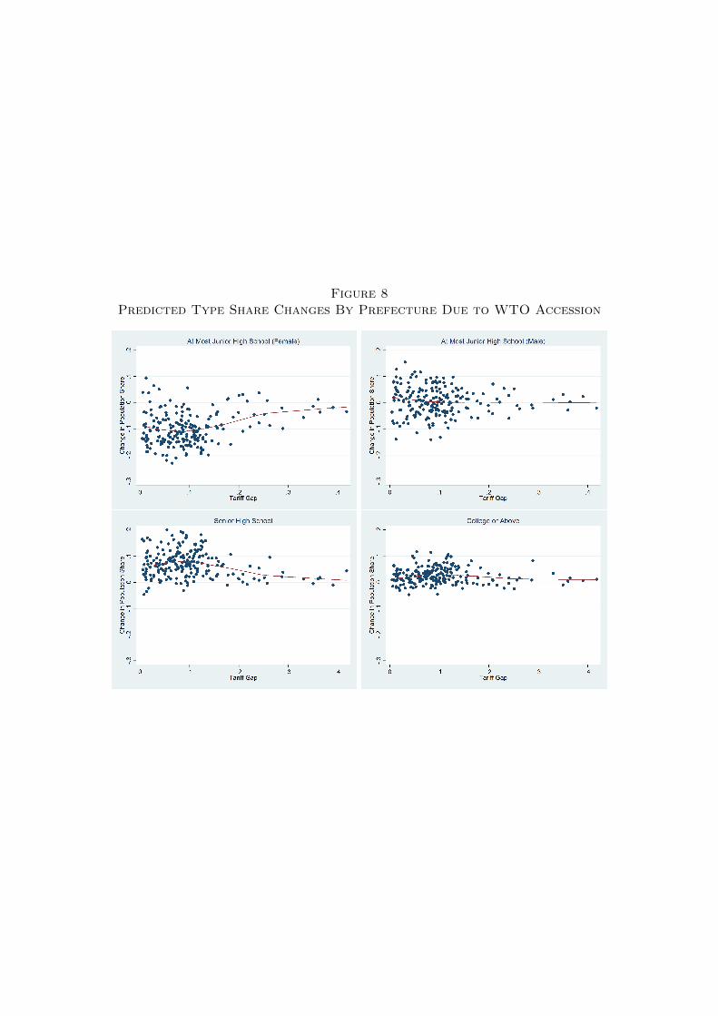
Figure 8Predicted Type Share Changes By Prefecture Due to WTO Accession

Supplemental Materials for Wenya Cheng and John Morrow

Firm Productivity Differences From Factor Markets

APPENDIX G

G(i). Supplemental Derivations

The expressions which fix the cutoff cost draw ηTR and mass of entry MTR can be neatly

summarized by defining the mass of entrants who produce, MTR, and the (locally weighted)

average cost draw in each region, ηTR:

MTR ≡MT

RG(ηTR), ηTR ≡

∫ ηTR

0

(ηTz u

TR

(UTR

)1/ρ)ρ/(ρ−1)

dG (z) /G(ηTR).

Using the profit maximizing price P TRj and combining Equations (9) and (10) then yields

the equilibrium quantity produced,

(1) QTRj = ρI

(uTRηj

(UTR/σ

TR

)1/ρ)ρ/(ρ−1)

/uTRηj∑t,r

(σtr)1/(1−ρ) Mt

rηtr.

Aggregating revenues using Equation (1) shows that each consumer’s budget share allo-

cated to region R and industry T is

(2) Consumer Budget Share for R,T :(σTR)1/(1−ρ) MT

RηTR/∑t,r

(σtr)1/(1−ρ) Mt

rηtr.

Consequently, since free entry implies expected profits must equal expected fixed costs,

the mass of entrants MTR solves the implicit form1

(3) (1− ρ) I

((σTR)1/(1−ρ) MT

RηTR/∑t,r

(σtr)1/(1−ρ) Mt

rηtr

)= MT

RuTR

(feG

(ηTR)

+ Fe),

1To see a solution exists, note that for fixed prices,{ηTR}

, and{ηTR}

, necessarily MTR ∈ ATR ≡[

0, (1− ρ) I/uTRFe]. Existence follows from the Brouwer fixed point theorem on the domain ×R,TATR for

H({

MTR

})≡ (1− ρ) I

((σTR)1/(1−ρ) MT

RηTR/∑t,r (σtr)

1/(1−ρ) Mtrηtr

)/uTR

(feG

(ηTR)

+ Fe).

1

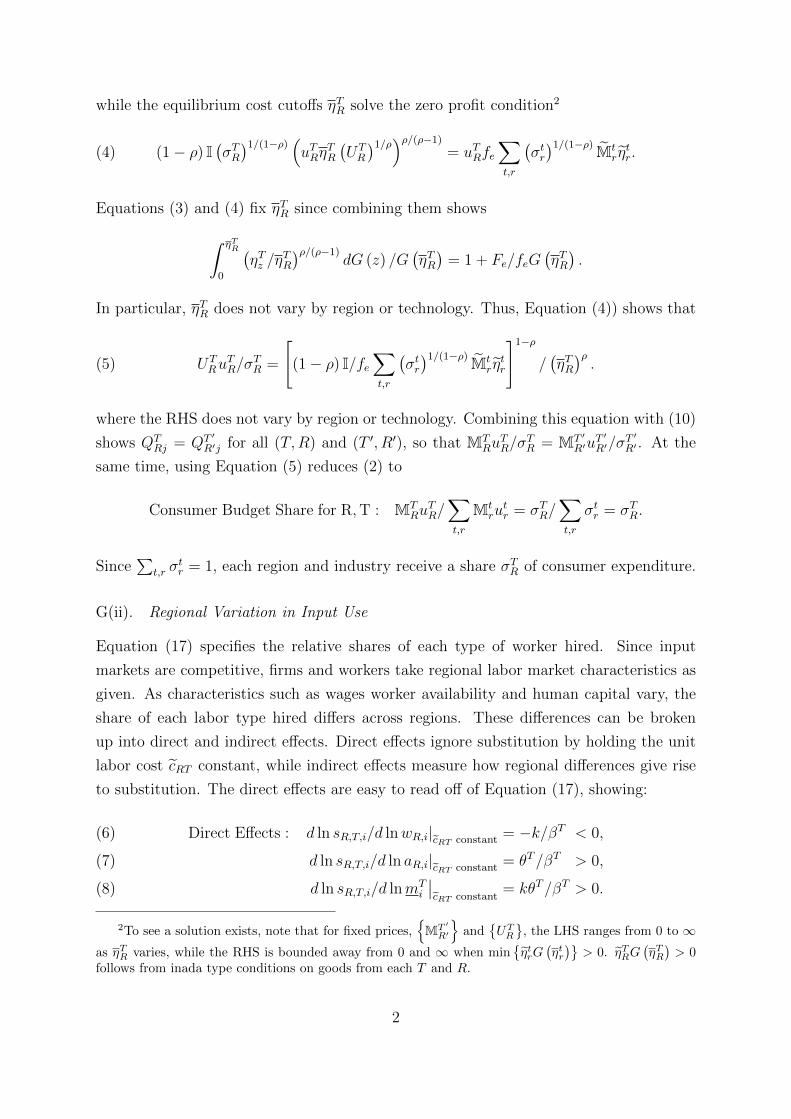
while the equilibrium cost cutoffs ηTR solve the zero profit condition2

(4) (1− ρ) I(σTR)1/(1−ρ)

(uTRη

TR

(UTR

)1/ρ)ρ/(ρ−1)

= uTRfe∑t,r

(σtr)1/(1−ρ) Mt

rηtr.

Equations (3) and (4) fix ηTR since combining them shows

∫ ηTR

0

(ηTz /η

TR

)ρ/(ρ−1)dG (z) /G

(ηTR)

= 1 + Fe/feG(ηTR).

In particular, ηTR does not vary by region or technology. Thus, Equation (4)) shows that

(5) UTRu

TR/σ

TR =

[(1− ρ) I/fe

∑t,r

(σtr)1/(1−ρ) Mt

rηtr

]1−ρ

/(ηTR)ρ.

where the RHS does not vary by region or technology. Combining this equation with (10)

shows QTRj = QT ′

R′j for all (T,R) and (T ′, R′), so that MTRu

TR/σ

TR = MT ′

R′uT′

R′/σT′

R′ . At the

same time, using Equation (5) reduces (2) to

Consumer Budget Share for R,T : MTRu

TR/∑t,r

Mtru

tr = σTR/

∑t,r

σtr = σTR.

Since∑

t,r σtr = 1, each region and industry receive a share σTR of consumer expenditure.

G(ii). Regional Variation in Input Use

Equation (17) specifies the relative shares of each type of worker hired. Since input

markets are competitive, firms and workers take regional labor market characteristics as

given. As characteristics such as wages worker availability and human capital vary, the

share of each labor type hired differs across regions. These differences can be broken

up into direct and indirect effects. Direct effects ignore substitution by holding the unit

labor cost cRT constant, while indirect effects measure how regional differences give rise

to substitution. The direct effects are easy to read off of Equation (17), showing:

Direct Effects : d ln sR,T,i/d lnwR,i|cRT constant = −k/βT < 0,(6)

d ln sR,T,i/d ln aR,i|cRT constant = θT/βT > 0,(7)

d ln sR,T,i/d lnmTi

∣∣cRT constant

= kθT/βT > 0.(8)

2To see a solution exists, note that for fixed prices,{MT ′

R′

}and

{UTR}

, the LHS ranges from 0 to ∞as ηTR varies, while the RHS is bounded away from 0 and ∞ when min

{ηtrG

(ηtr)}

> 0. ηTRG(ηTR)> 0

follows from inada type conditions on goods from each T and R.

2

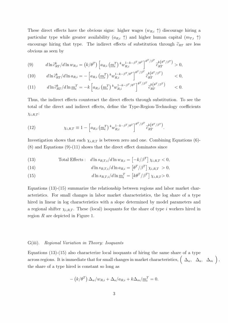
These direct effects have the obvious signs: higher wages (wR,i ↑) discourage hiring a

particular type while greater availability (aR,i ↑) and higher human capital (mT,i ↑)encourage hiring that type. The indirect effects of substitution through cRT are less

obvious as seen by

d ln ckRT/d lnwR,i =(k/θT

) [aR,i

(mTi

)kw

1−k−βT /θT

R,i

]θT /βT

ck(θT /βT )RT > 0,(9)

d ln ckRT/d ln aR,i = −[aR,i

(mTi

)kw

1−k−βT /θT

R,i

]θT /βT

ck(θT /βT )RT < 0,(10)

d ln ckRT/d lnmTi = −k

[aR,i

(mTi

)kw

1−k−βT /θT

R,i

]θT /βT

ck(θT /βT )RT < 0.(11)

Thus, the indirect effects counteract the direct effects through substitution. To see the

total of the direct and indirect effects, define the Type-Region-Technology coefficients

χi,R,T :

(12) χi,R,T ≡ 1−[aR,i

(mTi

)kw

1−k−βT /θT

R,i

]θT /βT

ck(θT /βT )RT .

Investigation shows that each χi,R,T is between zero and one. Combining Equations (6)-

(8) and Equations (9)-(11) shows that the direct effect dominates since

Total Effects : d ln sR,T,i/d lnwR,i =[−k/βT

]χi,R,T < 0,(13)

d ln sR,T,i/d ln aR,i =[θT/βT

]χi,R,T > 0,(14)

d ln sR,T,i/d lnmTi =

[kθT/βT

]χi,R,T> 0.(15)

Equations (13)-(15) summarize the relationship between regions and labor market char-

acteristics. For small changes in labor market characteristics, the log share of a type

hired in linear in log characteristics with a slope determined by model parameters and

a regional shifter χi,R,T . These (local) isoquants for the share of type i workers hired in

region R are depicted in Figure 1.

G(iii). Regional Variation in Theory: Isoquants

Equations (13)-(15) also characterize local isoquants of hiring the same share of a type

across regions. It is immediate that for small changes in market characteristics,(

∆w, ∆a, ∆m

),

the share of a type hired is constant so long as

−(k/θT

)∆w/wR,i + ∆a/aR,i + k∆m/m

Ti = 0.

3

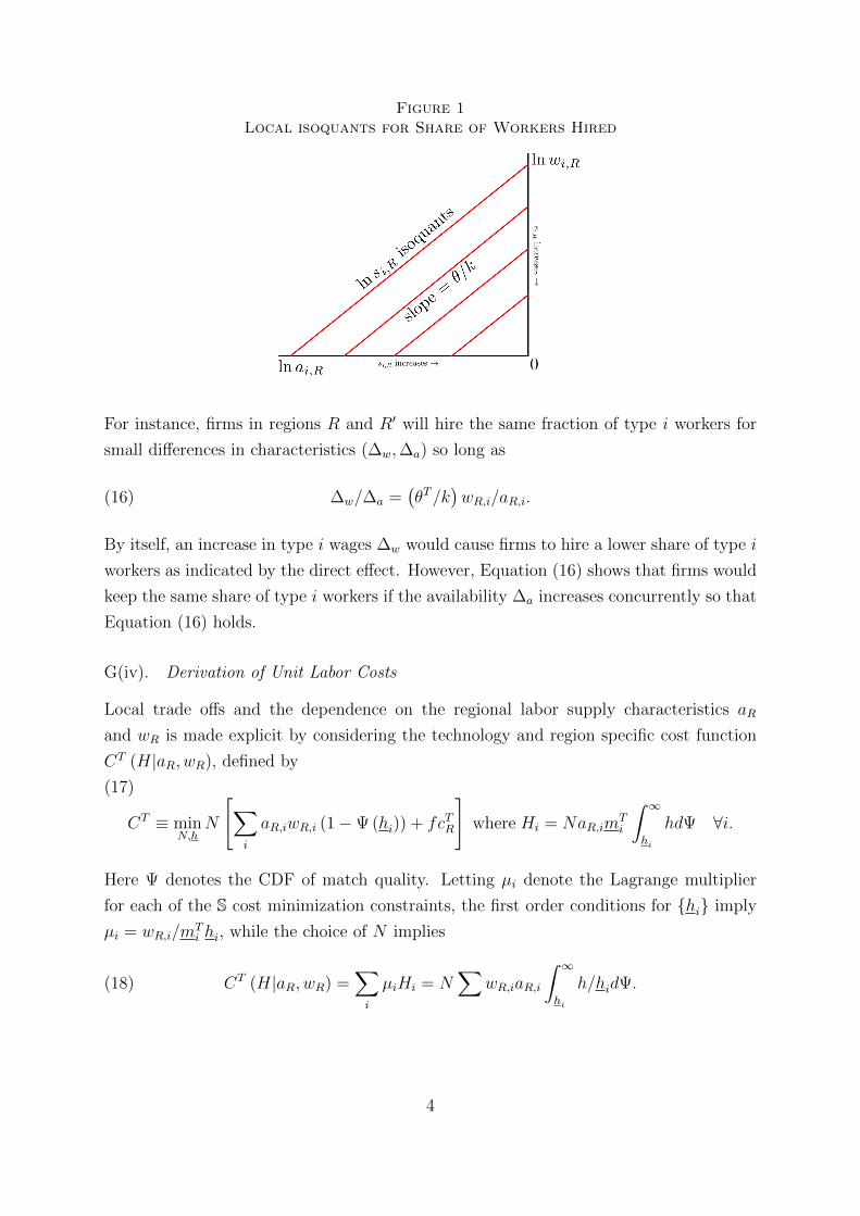
Figure 1Local isoquants for Share of Workers Hired

For instance, firms in regions R and R′ will hire the same fraction of type i workers for

small differences in characteristics (∆w,∆a) so long as

(16) ∆w/∆a =(θT/k

)wR,i/aR,i.

By itself, an increase in type i wages ∆w would cause firms to hire a lower share of type i

workers as indicated by the direct effect. However, Equation (16) shows that firms would

keep the same share of type i workers if the availability ∆a increases concurrently so that

Equation (16) holds.

G(iv). Derivation of Unit Labor Costs

Local trade offs and the dependence on the regional labor supply characteristics aR

and wR is made explicit by considering the technology and region specific cost function

CT (H|aR, wR), defined by

(17)

CT ≡ minN,h

N

[∑i

aR,iwR,i (1−Ψ (hi)) + fcTR

]where Hi = NaR,im

Ti

∫ ∞hi

hdΨ ∀i.

Here Ψ denotes the CDF of match quality. Letting µi denote the Lagrange multiplier

for each of the S cost minimization constraints, the first order conditions for {hi} imply

µi = wR,i/mTi hi, while the choice of N implies

(18) CT (H|aR, wR) =∑i

µiHi = N∑

wR,iaR,i

∫ ∞hi

h/hidΨ.

4

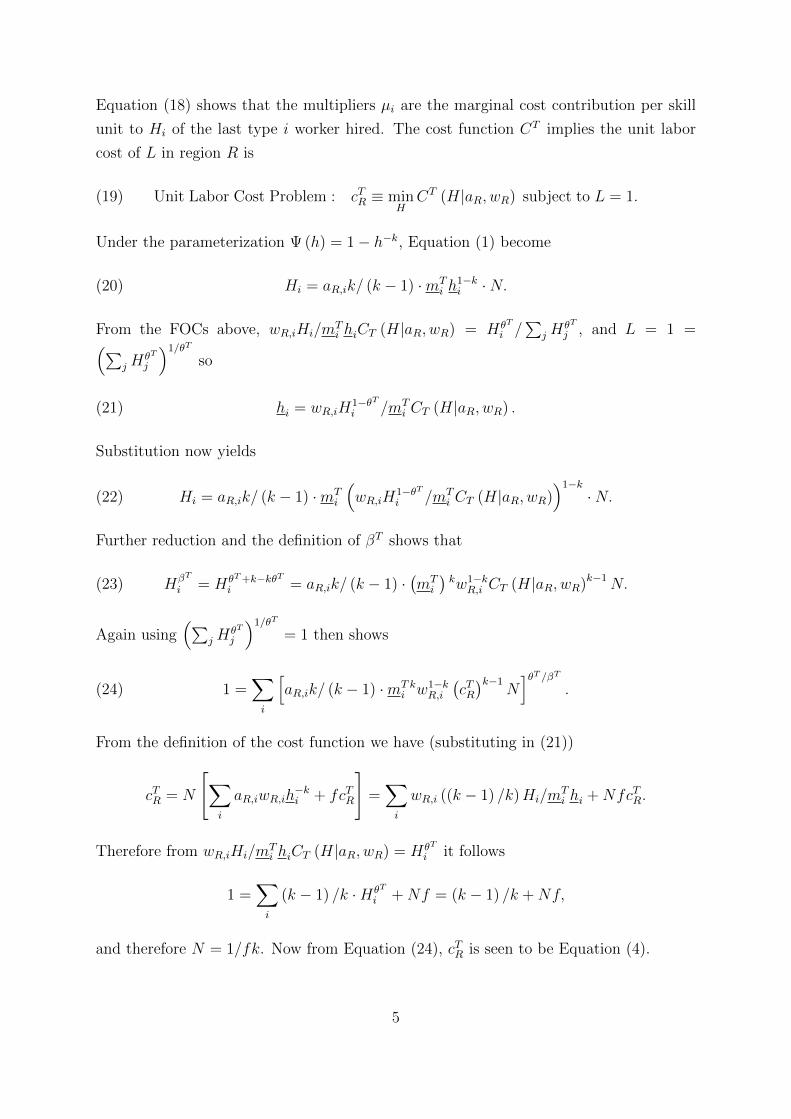
Equation (18) shows that the multipliers µi are the marginal cost contribution per skill

unit to Hi of the last type i worker hired. The cost function CT implies the unit labor

cost of L in region R is

(19) Unit Labor Cost Problem : cTR ≡ minH

CT (H|aR, wR) subject to L = 1.

Under the parameterization Ψ (h) = 1− h−k, Equation (1) become

(20) Hi = aR,ik/ (k − 1) ·mTi h

1−ki ·N.

From the FOCs above, wR,iHi/mTi hiCT (H|aR, wR) = HθT

i /∑

j HθT

j , and L = 1 =(∑j H

θT

j

)1/θT

so

(21) hi = wR,iH1−θTi /mT

i CT (H|aR, wR) .

Substitution now yields

(22) Hi = aR,ik/ (k − 1) ·mTi

(wR,iH

1−θTi /mT

i CT (H|aR, wR))1−k

·N.

Further reduction and the definition of βT shows that

(23) HβT

i = HθT +k−kθTi = aR,ik/ (k − 1) ·

(mTi

)kw1−k

R,i CT (H|aR, wR)k−1N.

Again using(∑

j HθT

j

)1/θT

= 1 then shows

(24) 1 =∑i

[aR,ik/ (k − 1) ·mT

ikw1−k

R,i

(cTR)k−1

N]θT /βT

.

From the definition of the cost function we have (substituting in (21))

cTR = N

[∑i

aR,iwR,ih−ki + fcTR

]=∑i

wR,i ((k − 1) /k)Hi/mTi hi +NfcTR.

Therefore from wR,iHi/mTi hiCT (H|aR, wR) = HθT

i it follows

1 =∑i

(k − 1) /k ·HθT

i +Nf = (k − 1) /k +Nf,

and therefore N = 1/fk. Now from Equation (24), cTR is seen to be Equation (4).

5

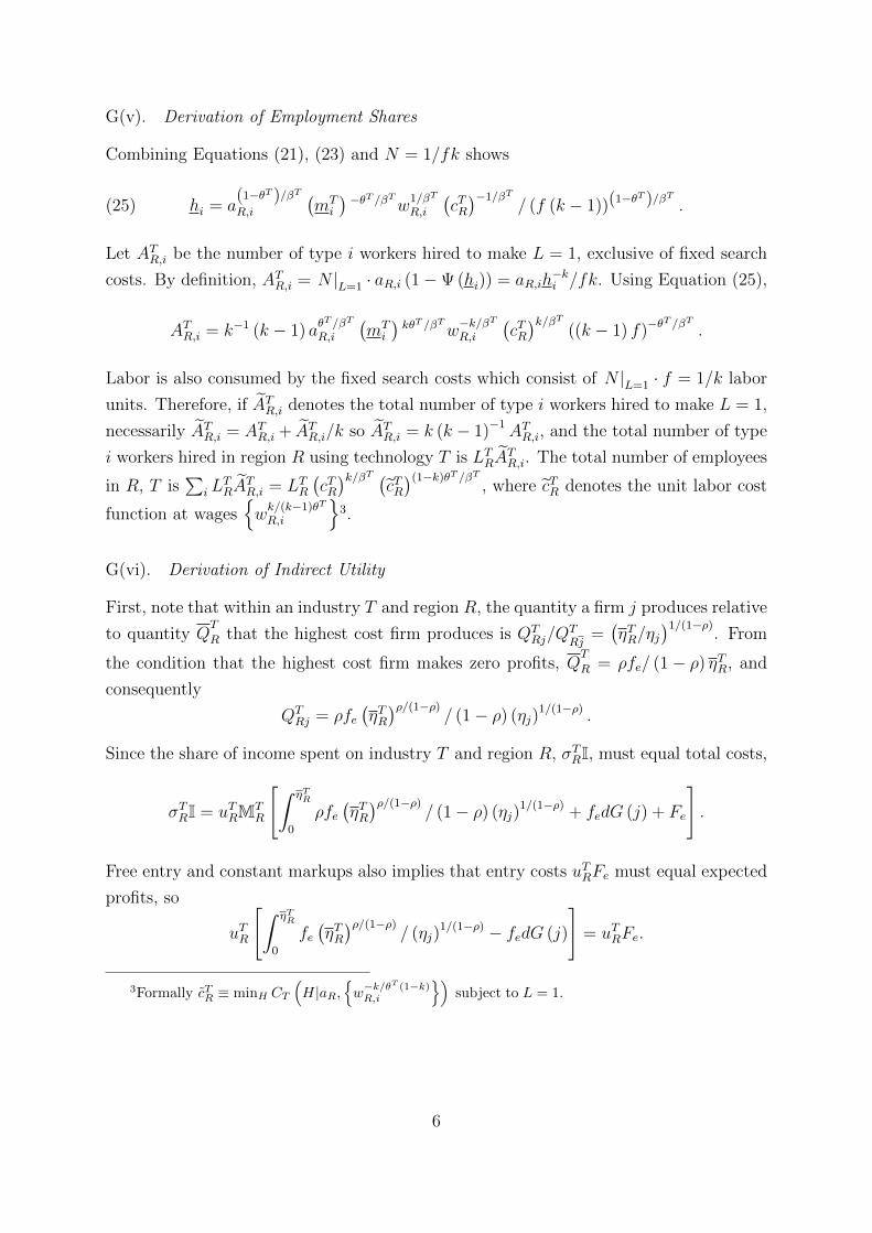
G(v). Derivation of Employment Shares

Combining Equations (21), (23) and N = 1/fk shows

(25) hi = a(1−θT )/βT

R,i

(mTi

) −θT /βT

w1/βT

R,i

(cTR)−1/βT

/ (f (k − 1))(1−θT )/βT

.

Let ATR,i be the number of type i workers hired to make L = 1, exclusive of fixed search

costs. By definition, ATR,i = N |L=1 · aR,i (1−Ψ (hi)) = aR,ih−ki /fk. Using Equation (25),

ATR,i = k−1 (k − 1) aθT /βT

R,i

(mTi

)kθT /βT

w−k/βT

R,i

(cTR)k/βT

((k − 1) f)−θT /βT

.

Labor is also consumed by the fixed search costs which consist of N |L=1 · f = 1/k labor

units. Therefore, if ATR,i denotes the total number of type i workers hired to make L = 1,

necessarily ATR,i = ATR,i + ATR,i/k so ATR,i = k (k − 1)−1ATR,i, and the total number of type

i workers hired in region R using technology T is LTRATR,i. The total number of employees

in R, T is∑

i LTRA

TR,i = LTR

(cTR)k/βT (

cTR)(1−k)θT /βT

, where cTR denotes the unit labor cost

function at wages{wk/(k−1)θT

R,i

}3.

G(vi). Derivation of Indirect Utility

First, note that within an industry T and region R, the quantity a firm j produces relative

to quantity QT

R that the highest cost firm produces is QTRj/Q

TRj

=(ηTR/ηj

)1/(1−ρ). From

the condition that the highest cost firm makes zero profits, QT

R = ρfe/ (1− ρ) ηTR, and

consequently

QTRj = ρfe

(ηTR)ρ/(1−ρ)

/ (1− ρ) (ηj)1/(1−ρ) .

Since the share of income spent on industry T and region R, σTRI, must equal total costs,

σTRI = uTRMTR

[∫ ηTR

0

ρfe(ηTR)ρ/(1−ρ)

/ (1− ρ) (ηj)1/(1−ρ) + fedG (j) + Fe

].

Free entry and constant markups also implies that entry costs uTRFe must equal expected

profits, so

uTR

[∫ ηTR

0

fe(ηTR)ρ/(1−ρ)

/ (ηj)1/(1−ρ) − fedG (j)

]= uTRFe.

3Formally cTR ≡ minH CT

(H|aR,

{w

−k/θT (1−k)R,i

})subject to L = 1.

6

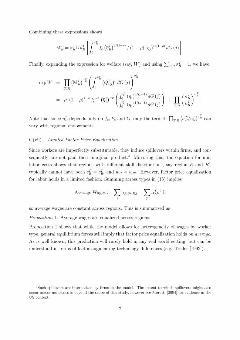
Combining these expressions shows

MTR = σTRI/uTR

[∫ ηTR

0

fe(ηTR)ρ/(1−ρ)

/ (1− ρ) (ηj)1/(1−ρ) dG (j)

].

Finally, expanding the expression for welfare (say, W ) and using∑

T,R σTR = 1, we have

expW =∏T,R

(MT

R

)σTR

(∫ ηTR

0

(QTRj

)ρdG (j)

)σTR

= ρρ (1− ρ)1−ρ fρ−1e

(η1

1

)−ρ(∫ η110(ηj)

ρ/(ρ−1) dG (j)∫ η110

(ηj)1/(ρ−1) dG (j)

)· I ·

∏T,R

(σTRuTR

)σTR

.

Note that since ηTR depends only on fe, Fe and G, only the term I ·∏

T,R

(σTR/u

TR

)σTR can

vary with regional endowments.

G(vii). Limited Factor Price Equalization

Since workers are imperfectly substitutable, they induce spillovers within firms, and con-

sequently are not paid their marginal product.4 Mirroring this, the equation for unit

labor costs shows that regions with different skill distributions, say region R and R′,

typically cannot have both cTR = cTR′ and wR = wR′ . However, factor price equalization

for labor holds in a limited fashion. Summing across types in (15) implies

Average Wages :∑i

aR,iwR,i =∑T

αTLσT I,

so average wages are constant across regions. This is summarized as

Proposition 1. Average wages are equalized across regions.

Proposition 1 shows that while the model allows for heterogeneity of wages by worker

type, general equilibrium forces still imply that factor price equalization holds on average.

As is well known, this prediction will rarely hold in any real world setting, but can be

understood in terms of factor augmenting technology differences (e.g. Trefler [1993]).

4Such spillovers are internalized by firms in the model. The extent to which spillovers might alsooccur across industries is beyond the scope of this study, however see Moretti [2004] for evidence in theUS context.

7

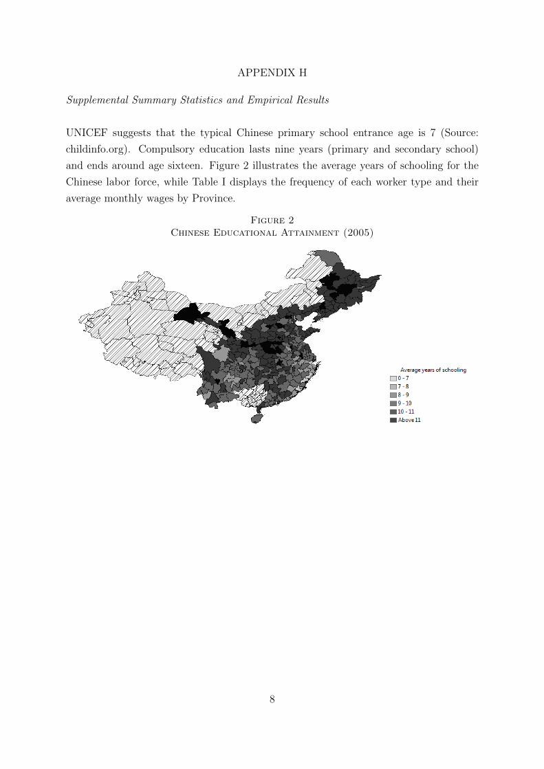
APPENDIX H

Supplemental Summary Statistics and Empirical Results

UNICEF suggests that the typical Chinese primary school entrance age is 7 (Source:

childinfo.org). Compulsory education lasts nine years (primary and secondary school)

and ends around age sixteen. Figure 2 illustrates the average years of schooling for the

Chinese labor force, while Table I displays the frequency of each worker type and their

average monthly wages by Province.

Figure 2Chinese Educational Attainment (2005)

8

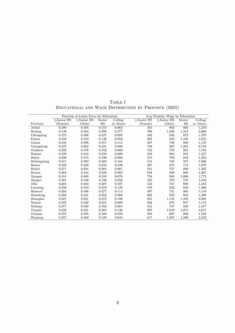
Table IEducational and Wage Distribution by Province (2005)

Fraction of Labor Force by Education Avg Monthly Wage by Education≤Junior HS ≤Junior HS Senior College ≤Junior HS ≤Junior HS Senior College

Province (Female) (Male) HS or Above (Female) (Male) HS or AboveAnhui 0.296 0.485 0.155 0.063 581 862 866 1,210Beijing 0.140 0.284 0.299 0.277 796 1,059 1,314 2,866Chongqing 0.272 0.408 0.227 0.093 582 820 872 1,379Fujian 0.348 0.453 0.146 0.052 695 942 1,103 1,855Gansu 0.216 0.399 0.271 0.114 507 738 869 1,135Guangdong 0.327 0.362 0.231 0.080 748 967 1,281 2,719Guizhou 0.292 0.478 0.162 0.069 572 758 925 1,189Hainan 0.328 0.334 0.259 0.080 532 694 894 1,527Hebei 0.230 0.515 0.190 0.066 515 793 832 1,233Heilongjiang 0.217 0.393 0.285 0.104 515 740 797 1,096Henan 0.229 0.428 0.234 0.109 487 675 714 1,079Hubei 0.271 0.384 0.264 0.081 541 757 809 1,262Hunan 0.263 0.444 0.229 0.063 634 828 889 1,267Jiangsu 0.314 0.400 0.210 0.076 758 994 1,086 1,773Jiangxi 0.291 0.456 0.196 0.056 525 783 794 1,240Jilin 0.204 0.382 0.307 0.107 522 745 809 1,163Liaoning 0.250 0.410 0.219 0.120 576 822 848 1,366Shaanxi 0.203 0.406 0.277 0.114 497 731 805 1,149Shandong 0.288 0.441 0.203 0.068 602 823 863 1,398Shanghai 0.221 0.321 0.272 0.186 891 1,155 1,450 3,085Shanxi 0.169 0.520 0.221 0.089 502 872 857 1,113Sichuan 0.277 0.480 0.162 0.081 541 737 829 1,477Tianjin 0.258 0.321 0.285 0.136 995 1,019 1,074 1,617Yunnan 0.275 0.495 0.160 0.070 504 697 896 1,542Zhejiang 0.357 0.469 0.129 0.045 817 1,097 1,299 2,333

9

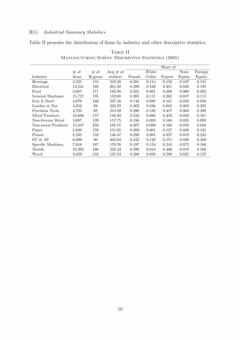
H(i). Industrial Summary Statistics

Table II presents the distribution of firms by industry and other descriptive statistics.

Table IIManufacturing Survey Descriptive Statistics (2005)

Share of# of # of Avg # of White State Foreign

Industry firms Regions workers Female Collar Export Equity EquityBeverage 2,225 155 219.20 0.281 0.114 0.150 0.107 0.121Electrical 12,241 166 201.58 0.289 0.106 0.351 0.030 0.195Food 3,807 171 193.98 0.321 0.091 0.266 0.060 0.202General Machines 15,727 195 152.68 0.205 0.117 0.262 0.047 0.115Iron & Steel 4,676 160 227.40 0.148 0.088 0.101 0.032 0.056Leather & Fur 4,852 89 320.70 0.362 0.036 0.682 0.005 0.335Precision Tools 2,702 68 214.89 0.296 0.180 0.457 0.063 0.299Metal Products 10,686 157 146.93 0.233 0.086 0.332 0.028 0.161Non-ferrous Metal 3,607 139 157.75 0.186 0.093 0.180 0.035 0.093Non-metal Products 15,347 259 195.57 0.207 0.090 0.169 0.059 0.088Paper 5,698 159 151.05 0.269 0.061 0.127 0.026 0.131Plastic 9,235 159 140.47 0.298 0.065 0.327 0.019 0.235PC & AV 6,699 90 402.04 0.342 0.120 0.571 0.038 0.459Specific Machines 7,816 167 176.76 0.197 0.154 0.244 0.072 0.166Textile 18,292 186 222.43 0.390 0.044 0.406 0.018 0.168Wood 3,629 133 137.04 0.288 0.050 0.290 0.025 0.137

10

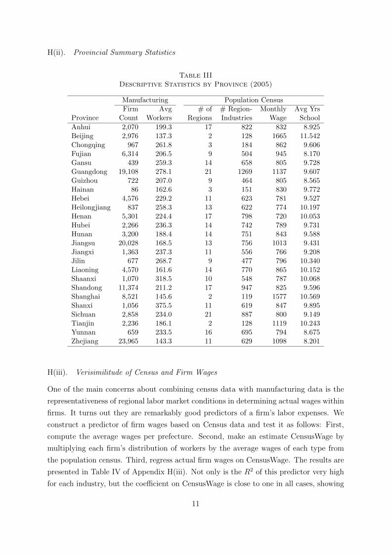
H(ii). Provincial Summary Statistics

Table IIIDescriptive Statistics by Province (2005)

Manufacturing Population CensusFirm Avg # of # Region- Monthly Avg Yrs

Province Count Workers Regions Industries Wage School

Anhui 2,070 199.3 17 822 832 8.925Beijing 2,976 137.3 2 128 1665 11.542Chongqing 967 261.8 3 184 862 9.606Fujian 6,314 206.5 9 504 945 8.170Gansu 439 259.3 14 658 805 9.728Guangdong 19,108 278.1 21 1269 1137 9.607Guizhou 722 207.0 9 464 805 8.565Hainan 86 162.6 3 151 830 9.772Hebei 4,576 229.2 11 623 781 9.527Heilongjiang 837 258.3 13 622 774 10.197Henan 5,301 224.4 17 798 720 10.053Hubei 2,266 236.3 14 742 789 9.731Hunan 3,200 188.4 14 751 843 9.588Jiangsu 20,028 168.5 13 756 1013 9.431Jiangxi 1,363 237.3 11 556 766 9.208Jilin 677 268.7 9 477 796 10.340Liaoning 4,570 161.6 14 770 865 10.152Shaanxi 1,070 318.5 10 548 787 10.068Shandong 11,374 211.2 17 947 825 9.596Shanghai 8,521 145.6 2 119 1577 10.569Shanxi 1,056 375.5 11 619 847 9.895Sichuan 2,858 234.0 21 887 800 9.149Tianjin 2,236 186.1 2 128 1119 10.243Yunnan 659 233.5 16 695 794 8.675Zhejiang 23,965 143.3 11 629 1098 8.201

H(iii). Verisimilitude of Census and Firm Wages

One of the main concerns about combining census data with manufacturing data is the

representativeness of regional labor market conditions in determining actual wages within

firms. It turns out they are remarkably good predictors of a firm’s labor expenses. We

construct a predictor of firm wages based on Census data and test it as follows: First,

compute the average wages per prefecture. Second, make an estimate CensusWage by

multiplying each firm’s distribution of workers by the average wages of each type from

the population census. Third, regress actual firm wages on CensusWage. The results are

presented in Table IV of Appendix H(iii). Not only is the R2 of this predictor very high

for each industry, but the coefficient on CensusWage is close to one in all cases, showing

11

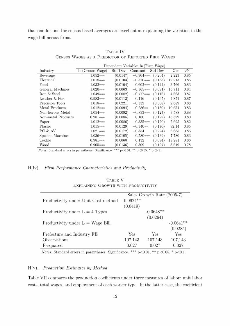
that one-for-one the census based averages are excellent at explaining the variation in the

wage bill across firms.

Table IVCensus Wages as a Predictor of Reported Firm Wages

Dependent Variable: ln (Firm Wage)Industry ln (Census Wage) Std Dev Constant Std Dev Obs R2

Beverage 1.052∗∗∗ (0.0147) −0.904∗∗∗ (0.204) 2,223 0.85Electrical 1.018∗∗∗ (0.0103) −0.370∗∗∗ (0.138) 12,213 0.86Food 1.032∗∗∗ (0.0104) −0.602∗∗∗ (0.144) 3,766 0.83General Machines 1.020∗∗∗ (0.0063) −0.365∗∗∗ (0.091) 15,711 0.84Iron & Steel 1.049∗∗∗ (0.0082) −0.777∗∗∗ (0.116) 4,663 0.87Leather & Fur 0.982∗∗∗ (0.0112) 0.116 (0.165) 4,851 0.87Precision Tools 1.018∗∗∗ (0.0221) −0.332 (0.308) 2,689 0.83Metal Products 1.012∗∗∗ (0.0094) −0.286∗∗ (0.130) 10,654 0.83Non-ferrous Metal 1.054∗∗∗ (0.0092) −0.833∗∗∗ (0.127) 3,588 0.88Non-metal Products 0.981∗∗∗ (0.0085) 0.160 (0.122) 15,329 0.80Paper 1.012∗∗∗ (0.0086) −0.335∗∗∗ (0.120) 5,695 0.82Plastic 1.015∗∗∗ (0.0129) −0.340∗∗ (0.170) 92,14 0.85PC & AV 1.021∗∗∗ (0.0172) −0.354 (0.224) 6,685 0.86Specific Machines 1.036∗∗∗ (0.0105) −0.580∗∗∗ (0.139) 7,780 0.83Textile 0.981∗∗∗ (0.0060) 0.132 (0.084) 18,281 0.86Wood 0.965∗∗∗ (0.0136) 0.309 (0.197) 3,619 0.78

Notes: Standard errors in parentheses. Significance. *** p<0.01, ** p<0.05, * p<0.1.

H(iv). Firm Performance Characteristics and Productivity

Table VExplaining Growth with Productivity

Sales Growth Rate (2005-7)Productivity under Unit Cost method -0.0924**

(0.0419)Productivity under L = 4 Types -0.0648**

(0.0264)Productivity under L = Wage Bill -0.0641**

(0.0285)Prefecture and Industry FE Yes Yes YesObservations 107,143 107,143 107,143R-squared 0.027 0.027 0.027

Notes: Standard errors in parentheses. Significance. *** p<0.01, ** p<0.05, * p<0.1.

H(v). Production Estimates by Method

Table VII compares the production coefficients under three measures of labor: unit labor

costs, total wages, and employment of each worker type. In the latter case, the coefficient

12

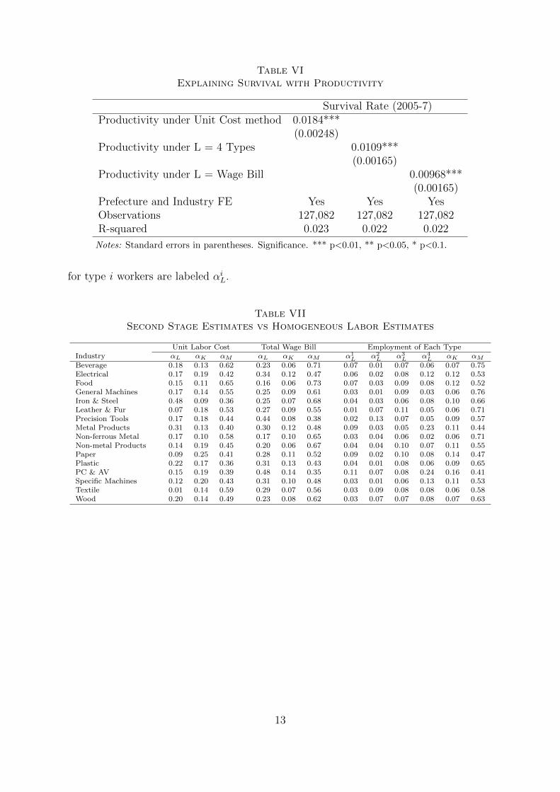
Table VIExplaining Survival with Productivity

Survival Rate (2005-7)Productivity under Unit Cost method 0.0184***

(0.00248)Productivity under L = 4 Types 0.0109***

(0.00165)Productivity under L = Wage Bill 0.00968***

(0.00165)Prefecture and Industry FE Yes Yes YesObservations 127,082 127,082 127,082R-squared 0.023 0.022 0.022

Notes: Standard errors in parentheses. Significance. *** p<0.01, ** p<0.05, * p<0.1.

for type i workers are labeled αiL.

Table VIISecond Stage Estimates vs Homogeneous Labor Estimates

Unit Labor Cost Total Wage Bill Employment of Each TypeIndustry αL αK αM αL αK αM α1

L α2L α3

L α4L αK αM

Beverage 0.18 0.13 0.62 0.23 0.06 0.71 0.07 0.01 0.07 0.06 0.07 0.75Electrical 0.17 0.19 0.42 0.34 0.12 0.47 0.06 0.02 0.08 0.12 0.12 0.53Food 0.15 0.11 0.65 0.16 0.06 0.73 0.07 0.03 0.09 0.08 0.12 0.52General Machines 0.17 0.14 0.55 0.25 0.09 0.61 0.03 0.01 0.09 0.03 0.06 0.76Iron & Steel 0.48 0.09 0.36 0.25 0.07 0.68 0.04 0.03 0.06 0.08 0.10 0.66Leather & Fur 0.07 0.18 0.53 0.27 0.09 0.55 0.01 0.07 0.11 0.05 0.06 0.71Precision Tools 0.17 0.18 0.44 0.44 0.08 0.38 0.02 0.13 0.07 0.05 0.09 0.57Metal Products 0.31 0.13 0.40 0.30 0.12 0.48 0.09 0.03 0.05 0.23 0.11 0.44Non-ferrous Metal 0.17 0.10 0.58 0.17 0.10 0.65 0.03 0.04 0.06 0.02 0.06 0.71Non-metal Products 0.14 0.19 0.45 0.20 0.06 0.67 0.04 0.04 0.10 0.07 0.11 0.55Paper 0.09 0.25 0.41 0.28 0.11 0.52 0.09 0.02 0.10 0.08 0.14 0.47Plastic 0.22 0.17 0.36 0.31 0.13 0.43 0.04 0.01 0.08 0.06 0.09 0.65PC & AV 0.15 0.19 0.39 0.48 0.14 0.35 0.11 0.07 0.08 0.24 0.16 0.41Specific Machines 0.12 0.20 0.43 0.31 0.10 0.48 0.03 0.01 0.06 0.13 0.11 0.53Textile 0.01 0.14 0.59 0.29 0.07 0.56 0.03 0.09 0.08 0.08 0.06 0.58Wood 0.20 0.14 0.49 0.23 0.08 0.62 0.03 0.07 0.07 0.08 0.07 0.63

13