Embed Size (px)
Citation preview

Chen, Jingsi (2010) Towards single photon detection with a practical EMCCD. MSc(Res) thesis, University of Nottingham.
Access from the University of Nottingham repository: http://eprints.nottingham.ac.uk/11251/1/Jingsi_Chen_Final_thesis.pdf
Copyright and reuse:
The Nottingham ePrints service makes this work by researchers of the University of Nottingham available open access under the following conditions.
This article is made available under the University of Nottingham End User licence and may be reused according to the conditions of the licence. For more details see: http://eprints.nottingham.ac.uk/end_user_agreement.pdf
For more information, please contact [email protected]
THE UNIVERSITY OF NOTTINGHAM
SCHOOL OF ELECTRICAL AND
ELECTRONIC ENGINEERING
Towards single photon detection
with a practical EMCCD
Author: Jingsi Chen
Supervisor: Mike Somekh
Thesis submitted to the University of Nottingham for the degree of
MSc (by research)
DECEMBER 2009

Abstract
The stochastic transfer function (STF) is a metric for imaging of a microscope that
includes the idea of noise, this project attempted to obtain the STF by Monte Carlo
method with photon counting device. In this project, a very sensitive Electron-
multiplying CCD (EMCCD) camera is evaluated for its photon counting performance
on STF measurement. The evaluation system employs a beam with a very weak
intensity laser to illuminate the EMCCD, the output signal and background noise of the
EMCCD is recorded and statistical data is obtained. The EMCCD output signal
distribution under different conditions is given by a simulation. Moreover, photon
counting in TIRF with fluorescent beads is also carried out to simulate the practical STF
measurement condition. Although the experiment results suggest that the EMCCD
camera used in this project is not capable of performing photon counting for the Monte
Carlo method, the performance of this EMCCD camera is studied in detail. The
evaluation method and data can be used to evaluate other EMCCD or photon counting
devices.

Acknowledgements
I would like to thank my supervisor Professor Mike Somekh for his invaluable help and
advice throughout this year, without his support and supervision this project could not
be accomplished. I would also like to thank Dr. Chung See, Dr. Mark Pitter and Gerard
Byrne for their advice and support.
I would also like to thank my friends and laboratory colleagues Lin Wang, Bo Fu, Ken
Hsu, Stephen, Shugang Liu and Jing Zhang for their help and support. Thanks to all
other persons who provided help for the project.
Finally, I would like to thank my parents for their support and encourage throughout my
study.

List of contents
Chapter 1 Introduction............................................................................................... 1
1.1 Point Spread Function and Optical Transfer Function.................................... 3 1.1.1 Point Spread Function............................................................................ 3 1.1.2 Resolution ............................................................................................. 5 1.1.3 Optical Transfer Function ...................................................................... 7
1.2 Stochastic transfer function and photon counting........................................... 8 1.2.1 Stochastic transfer function.................................................................... 9 1.2.2 Experimental verification for the STF.................................................. 10
1.3 CCD............................................................................................................ 11 1.3.1 Structure of CCD................................................................................. 11 1.3.2 CCD Architecture................................................................................ 17 1.3.3 Noise in CCD ...................................................................................... 19
1.4 Electron-multiplying CCD (EMCCD) ......................................................... 22 1.4.1 Structure of EMCCD ........................................................................... 22 1.4.2 Noise in EMCCD ................................................................................ 23
1.5 TIRF ........................................................................................................... 25 Chapter 2 Measurement system and EMCCD camera optimization.......................... 29
2.1 Measurement system configuration ............................................................. 29 2.2 Camera optimization and EM gain calibration ............................................. 33
2.2.1 Camera optimization............................................................................ 34 2.2.2 EM gain calibration ............................................................................. 39 2.2.3 Choosing a suitable EM gain value ...................................................... 41
Chapter 3 Evaluating photon counting performance of EMCCD.............................. 44 3.1 Principle of photon counting by EMCCD .................................................... 44 3.2 Method........................................................................................................ 45 3.3 Result and data analysis............................................................................... 48
3.3.1 Probability density distribution ............................................................ 48 3.3.2 Cumulative distribution ....................................................................... 52 3.3.3 Estimation of the CDF of one photon................................................... 56 3.3.4 Simulation of signal distribution .......................................................... 58 3.3.5 Conclusion .......................................................................................... 66
Chapter 4 Photon counting with flourophore in TIRF .............................................. 68 4.1 Instrument configuration ............................................................................. 68 4.2 Method........................................................................................................ 70 4.3 Analysis of results ....................................................................................... 74
Chapter 5 Conclusion .............................................................................................. 83 5.1 Summary and conclusion............................................................................. 83 5.2 Other devices which might have better performance.................................... 85
5.2.1 Back-illuminated EMCCD................................................................... 85 5.2.2 PMT .................................................................................................... 87 5.2.3 ICCD................................................................................................... 88
References ............................................................................................................... 89

Chapter 1
Page 1
Chapter 1 Introduction
The stochastic transfer function (STF) is a metric for imaging of a
microscope that includes the idea of noise. The original objective of the
project was to obtain an experimental verification of STF by Monte Carlo
method with an Electron-multiplying CCD (EMCCD) camera which acts
as a photon counting device. The EMCCD used in the project was
supposed to be very sensitive and able to perform photon counting.
However, during the project the EMCCD is found to be not as sensitive as
the manufacturer claims, the noise of the EMCCD became a problem in
photon counting, especially at very low light intensity. Therefore the
objective of the project is altered to evaluating the EMCCD for its photon
counting performance on STF measurement.
A system is build to evaluate the EMCCD, in the system a beam of laser
which is expanded and attenuated illuminates the EMCCD, the power of
laser is measured by power meter so the photon mean number on each
pixel of EMCCD during an exposure is known. The EMCCD output signal
under different photon mean number and the effect of noise are studied and
a simulation of probability distribution of signal and noise is performed.
Moreover, the EMCCD is used for photon counting in TIRF (Total internal
reflection fluorescence microscopy) with fluorescent beads is also carried
out to simulate the practical STF measurement condition. According to the

Chapter 1
Page 2
experimental results, the EMCCD camera used in this project is not
capable of performing photon counting for the Monte Carlo method.
Content of the thesis:
Chapter 1: Introduction of point spread function, transfer function,
stochastic transfer function, CCD, EMCCD and TIRF.
Chapter 2: The configuration of measurement system for EMCCD
evaluation. The EMCCD is optimized before the experiment.
Chapter 3: The experimental method for EMCCD evaluation. The
statistical data of EMCCD output signal is obtained, the probability density
distribution and cumulative distribution is studied, a simulation of signal
and noise probability distribution is performed based on experiment data.
Chapter 4: EMCCD photon counting in TIRF with fluorescent beads. The
practical STF measurement is to be performed in TIRF with small
fluorescent beads as point sources, and this experiment is to simulate
photon counting in practical conditions. The experimental result obeys the
previous simulation prediction.
Chapter 5: Summary and some suggestions for other photon devices.

Chapter 1
Page 3
1.1 Point Spread Function and Optical Transfer
Function
1.1.1 Point Spread Function
The point spread function (PSF) describes the response of an imaging
system to a point source or point object. Due to the diffraction, the image
of an object formed by an optical imaging system cannot be exactly the
same as the object.
A point source in an imaging system can be seen as an impulse function in
linear system theory, and the PSF is an imaging system's impulse response.
In a linear system, the system output is the convolution of input with
system impulse response. It is similar in an imaging system, the image of a
object is the convolution of the object itself with the PSF of the imaging
system.
As the PSF is entirely determined by the imaging system, the degree of
spreading of the PSF is a measure for the quality of an imaging system.
For a conventional light microscope, the PSF is a jinc function. The jinc
function is defined as
xxJx )()(jinc 1
= (1.1)
where J1(x) is a Bessel function of the first kind.

Chapter 1
Page 4
The width between two first zeros of PSF is:
NAλ22.1 (1.2)
where λ is the light wavelength and NA is the numerical aperture of a
microscope objective. NA is defined as the sine of the half-angle of the
maximum cone of light that can enter or exit the lens multiplied by the
refraction index of the medium in which the lens is working.
θsinnNA = (1.3)
It is obvious that the higher NA, the smaller width of the PSF. (Figure 1.1)
Figure 1.1 Point Spread Function (PSF), Two PSFs are shown, one for high
numerical aperture (NA=1.3 in grey) and one for NA=0.3 (slightly
transparent shades) [1]

Chapter 1
Page 5
1.1.2 Resolution
The resolution of a microscope objective is defined as the smallest distance
between two points on a specimen that can still be distinguished as two
separate entities. Resolution is a somewhat subjective value in microscopy,
because the precise values of the resolution we obtained depends on the
exact criterion and the signal to noise ratio (SNR).
SNR is usually not considered as a factor of resolution since the light signal
is usually strong enough and SNR is usually high in normal conditions,
however, when light is very weak, the SNR become an important factor of
resolution. Two close points might be distinguished as two separate entities
on an image with high SNR, but might not be distinguished in the case of
low SNR because of the effect of noise.
The Rayleigh resolution limit defines resolution using the example of two
point objects: The images of two different points are regarded as just
resolved when the principal diffraction maximum of one image coincides
with the first minimum of the other. If the distance is greater, the two
points are well resolved and if it is smaller, they are not resolved. (Figure
1.2)

Chapter 1
Page 6
The diffraction limit given by the Rayleigh criterion is:
NAd λ61.0min = (1.4)
To increase the lateral resolution of the imaging system, the value of dmin
needs to be decreased. This can be achieved by reducing the illumination
wavelength or increasing the NA of the objectives. Usually visible light is
used for illumination and the wavelength ranges from about 380 to 750 nm.
Figure 1.2 Rayleigh criterion. Two point objects are resolved when
diffraction maximum of one image coincides with the first minimum
of the other.

Chapter 1
Page 7
As θsinnNA = , the maximum value of sinθ is 1, the NA of dry objective
(which use air as imaging medium) cannot be greater than 1, and it is
difficult to achieve NA above 0.95 in practice. For oil immersion objective,
the maximum NA is usually around 1.5.
For example, at λ=400nm using a 1.49 NA objective, the lateral resolution
is about 164nm according to Rayleigh criterion.
1.1.3 Optical Transfer Function
From another point of view, an optical imaging system performs as a low
pass filter in spatial frequency domain. A higher resolution means more
fine detail and higher frequency component, thus a microscope system with
higher resolution has a higher bandwidth.
Like a linear system, the character of an optical system can be depicted by
a transfer function (or optical transfer function, OTF). The transfer function
describes the spatial variation as a function of spatial (angular) frequency,
it can be derived from the Fourier transform of the point spread function.
The transfer function is an important metric for microscope system. The
performance a microscope can be obtained by measuring its transfer
function. The transfer function can also be used to compare the
performance of different microscopes

Chapter 1
Page 8
1.2 Stochastic transfer function and photon counting
As the transfer function describes the character of a microscope system, it
is an important mean of comparing microscope performance. However,
conventional transfer function, which is essentially the mean or average
value we would expect to recover from a measurement, does not take into
account the signal-to-noise ratio (SNR) which can affect image quality
significantly, especially in conditions of weak signal.
For example, in the application of confocal fluorescence microscopes, a
small confocal detection pinhole improves lateral resolution; however it
reduces the SNR as fewer photons are detected, so this can result in a noisy
image.
Since most fluorophores can only produce a finite number of photons
(around 105 typically) before they photobleach, the trade-off between
resolution and the number of photons detected is very important in
fluorescence microscopy.
It is clear that an optimized microscope should not only provide good
lateral resolution but also make the best possible use of the detected
photons.

Chapter 1
Page 9
1.2.1 Stochastic transfer function
Recently the concept of the stochastic transfer function (STF) is introduced
as a metric for imaging of a microscope that includes the idea of noise. [2]
The stochastic transfer function encapsulates the ideas by presenting a
probability distribution for each spatial frequency. In contrast to the
conventional transfer function which represents only the mean or expected
value, the stochastic transfer function includes the noise or the variance at
each spatial frequency. Ideally, it would provide a complete probability
density function corresponding to each spatial frequency.
It will be very useful to have a quantitative measure of both the signal and
the noise in the image, and some theoretical work [2] that leads to this idea
has been done. The stochastic transfer function can be calculated in two
different ways, the first method is to calculate analytically using
characteristic function, and the other way is to obtain by Monte Carlo
method.
In the Monte Carlo method we consider a point object, decide the total
expected number of photons in the point spread function, and divide the
image of PSF into small regions. For each small region, the mean value in
the region is calculated, and a random number from a Poisson distribution
with the expected mean value is selected. After the data of the whole PSF
is collected, the data is Fourier transformed and a transfer function is
obtained. The process is repeated many times so that the mean and variance
Chapter 1
Page 10
of distribution at each spatial frequency can be recovered. This process will
be the exact procedure we use to extract the STF experimentally.
1.2.2 Experimental verification for the STF
The initial objective of this project was to attempt to give an experimental
verification for the STF by a TIRF microscope and the procedure is very
similar as described above. In the longer term it was hoped to extend it to
structured light microscopy.
An image of a small fluorophore (for example, a very small fluorescent
bead) formed by a microscope is divided into small segments and detected
by a detector or detector array. The magnification of the image must be
adjusted so that the size of the detector is small compared to the point
spread function.
The detector is used in photon counting mode, and the number of photons
in each small segment is recorded, and the data of photon number is
Fourier transformed. The process is repeated many times, and the mean and
variance of each spatial frequency is obtained from experiment result, thus
the experimentally determined value of the STF could be obtained.
In this project, a very sensitive electron-multiplying CCD (EMCCD)
camera, a device employs electron multiplication to amplify signal, is used
for photon counting. However, in the project the performance of the

Chapter 1
Page 11
EMCCD camera appears not as good as the manufacturer claims, so the
goal of the project became evaluating the performance of the EMCCD
camera and determining whether it is capable of photon counting for STF
measurement.
1.3 CCD
1.3.1 Structure of CCD
A CCD chip is an array of tiny light-sensitive elements called picture
elements, or pixels. Pixels are defined in the silicon matrix by an
orthogonal grid of narrow transparent electrode strips, or gates, deposited
on the chip. A thin layer of silicon dioxide (insulator) is placed on top of
the electrodes. Above the silicon dioxide is a layer of n-type silicon.
Finally, a thin layer of p-type silicon lies atop the n-type silicon, this
creates a p-n junction that covers the electrodes (Fig. 1.3 and 1.4). The p-n
junction is reverse biased.
Figure 1.3 Structure of CCD

Chapter 1
Page 12
The fundamental light-sensing unit of the CCD is a metal oxide
semiconductor (MOS) capacitor operated as a photodiode and storage
device (Figure 1.5).
If a photon with sufficient energy is incident on the P-N junction, it can be
absorbed, resulting in liberation of electrons, and an electron-hole pair is
created within the silicon crystal lattice. The negatively charged electrons
are collected by the positively charged gate electrode. Because one
electron-hole pair is generated by one absorbed photon, the charge
collected by the electrode is linearly proportional to the number of incident
photons. Thus the light flux on a pixel can be determined by measuring the
charge collected by the electrode.
Figure 1.4 Structure of CCD, side view.

Chapter 1
Page 13
After the charge created by photons is collected, it needs to be transferred
and measured. During transfer, charge is moved across the device by
manipulating voltages on the capacitor gates in a pattern that causes charge
to spill from one MOS capacitor to the next. The shift of charge within the
silicon is effectively coupled to clocked voltage patterns applied to the
overlying electrode structure, the basis of the term "charge-coupled" device.
Figure 1.5 Structure of metal oxide semiconductor (MOS)
capacitor. [3]
Figure 1.6 Structure of CCD sense element (pixel) [3]

Chapter 1
Page 14
The most common charge transfer configuration is the three-phase CCD
design, in which each pixel is divided into thirds with three parallel
potential wells defined by gate electrodes (Figure 1.6).
Once trapped in a potential well, electrons are moved across each pixel in a
three-step process (three-phase transfer) that shifts the charge packet from
one pixel row to the next. A sequence of voltage changes applied to
alternate electrodes of the parallel (vertical) gate structure move the
potential wells and the trapped electrons under control of a parallel shift
register clock, as shown in Figure 1.7.
The charge packages are vertically shifted row by row to the bottom row
called the readout register, or horizontal shift register. In the horizontal
shift register, charge packages are shifted one by one horizontally to output
gate for amplification, measurement, and analogue-to-digital conversion
(Figure 1.8).

Chapter 1
Page 15
Full-well capacity
The full-well capacity of a CCD pixel is the maximum number of photo-
electrons it can store before saturating. This full-well capacity determines
Figure 1.7 Three Phase CCD clocking schema. [3]
Figure 1.8 CCD readout schema. [4]

Chapter 1
Page 16
the maximum signal that can be sensed in the pixel, and is a primary factor
affecting the CCD's dynamic range. Full well capacity is mainly
determined by physical size of the individual pixel, generally, the bigger
the pixel, the larger the full-well capacity.
Fill factor
Fill factor never reach to 100% as some of the sensor surface is required
for control electronics. To improve the effective FF, some sensors use tiny
microlenses over each pixel to gather some of the light that would
otherwise have missed the photosensitive region.
Quantum efficiency
Quantum efficiency (QE) is defined as the percentage of incident photons
with a particular wavelength generating electron-hole pairs which
subsequently contribute to the output signal.
The parameter represents the effectiveness of a CCD imager in generating
charge from incident photons, and is therefore a major determinant of the
minimum detectable signal for a camera system, particularly when
performing low-light-level imaging.
Conventional front-illuminated CCD normally have QE of 40-60%, with
peak sensitivity normally in the range of 550-800nm, while the new back-
illuminated CCD may reach maximum 90% QE.

Chapter 1
Page 17
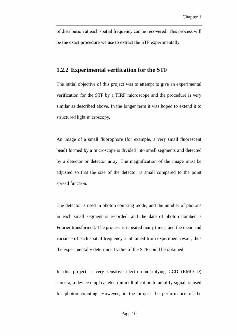
1.3.2 CCD architecture
There are three basic variations of CCD architecture in common use: full
frame, frame transfer, and interline transfer.
1.3.2.1 Full-frame CCD
The full-frame CCD, which employs the readout procedure described
previously, has the advantage of high fill factor, with virtually no dead
space between pixels. When full-frame CCD transfers the charge, the pixel
is busy and cannot continue to capture photons. Therefore a mechanical
shutter is usually used to protect the image area from incident light during
readout.
The shutter is opened during exposure and charge is accumulated in pixels,
then charge is transferred and read out after the shutter is closed. Because
the two steps cannot occur simultaneously, image frame rates are limited
by the mechanical shutter speed, the charge-transfer rate, and readout steps.
1.3.2.2 Frame-transfer CCD
Frame-transfer CCDs are similar to full-frame CCDs, but half of the array
is covered by an opaque mask to provide temporary storage for the charges
gathered by the unmasked light-sensitive portion. After image exposure,
the charge accumulated in photosensitive pixels is quickly transferred to
the storage array, typically within approximately 1 millisecond. As the
storage array is covered by an opaque mask, stored charge can be read out

Chapter 1
Page 18
at a slower speed while the next image is being exposed simultaneously in
light-sensitive array. Because frame-transfer CCDs are able to operate
continuously without mechanical shutter, they can operate at faster frame
rates than full-frame. A disadvantage of frame-transfer CCDs is that a
much larger chip is required as only one-half of the surface area of the
CCD is used for imaging, and larger chip also result in higher cost.
1.3.2.3 Interline CCD
In an interline CCD, each pixel has both a photo detector and a charge
storage area. The storage area is formed by masking part of the pixel from
light and using it only for the charge transfer process. The masked areas for
each pixel form a vertical charge transfer channel that runs from the top of
the array to the horizontal shift register.
Because a charge-transfer channel is located immediately adjacent to each
photosensitive pixel column, charge accumulated by photosensitive pixels
can be very quickly shifted to adjacent masked storage area, and then the
charge can be shifted down row by row to the horizontal shift register
while the image array is being exposed for the next image. Thus interline
CCD can operate at high frame rate without mechanical shutter.
The disadvantage of interline CCD is that a significant portion of the
sensor is no longer photosensitive, resulting in lower fill factor and hence
reduced dynamic range, resolution, and sensitivity. To overcome this
Chapter 1
Page 19
problem, interline CCDs often use microlenses to increase effective fill
factor.
1.3.3 Noise in CCD
There are three main noise sources in CCDs: photon shot noise, dark
current and readout noise.
1.3.3.1 Photon shot noise
Photon shot noise is an inherent noise source associated with the signal, it
is due to random variations of the photon flux.
Photon shot noise obeys Poisson distribution, it is equal to the square root
of the number of signal photons, N.
NSN =σ (1.5)
Figure 1.9 Common CCD architecture. (a) Full-frame. (b)Frame transfer.
(c)Interline transfer. [3]

Chapter 1
Page 20
Since it cannot be eliminated, photon shot noise determines the maximum
achievable SNR for a noise-free detector.
Signal to shot noise ratio (SSNR):
NN
NSSNR == (1.6)
It is obvious that full-well capacity is important to the SSNR. The larger
full-well capacity gives a higher SSNR, provide there is sufficient light fill
in the well.
1.3.3.2 Dark noise
Dark noise in CCD is noise detected in absence of light ,it is due to kinetic
vibrations of silicon atoms in the CCD substrate that generate free electrons
or holes even when the device is in total darkness, and it represents the
uncertainty in the magnitude of dark charge accumulation during a
specified time interval. The rate of generation of dark charge is termed dark
current. Dark noise also follows a square-root relationship to dark current,
and therefore it cannot simply be subtracted from the signal.
Dark noise is a source of noise in all semiconductor photo detectors. It can
be accurately calculated for CCDs from the following equations:
kTEdcs
geTNPD 25.115105.2 −×= (1.7)

Chapter 1
Page 21
where D is the dark current in electrons per sec per pixel, Eg is the silicon
bandgap energy (eV), T is absolute temperature (K), Ps is the pixel size
(cm2), Ndc is the dark current at 300k (nA/cm2, supplied by the
manufacturer) and k is Boltzmann’s constant (8.62x10⁻⁵ eV/K).
Dark current is unrelated to photon-induced signal but is highly
temperature dependent, so cooling the CCD has a dramatic effect on
reducing dark current. At -30 degrees, dark noise is reduced to 0.1~1
electron per pixel per second, and it is negligible for microscopy
applications.
1.3.3.3 Readout noise
When the signal on CCD is read out, charge packages are converted to
voltage signal and amplified. The noise in any amplifier is proportional to
B1/2, where B is system bandwidth. Generally, readout noise increases with
the speed of read out. Although the readout noise is added uniformly to
every pixel of the detector, its magnitude cannot be precisely determined,
but only approximated by an average value, in units of electrons (root-
mean-square or rms) per pixel.
Some good quality CCDs have readout noise less than 20 electrons. In this
case, photon shot noise, rather than readout noise, is a dominant noise
source when the signal is not very weak.

Chapter 1
Page 22
For extremely weak signals, this readout noise becomes a main noise
source, and some technology, such as ICCD and EMCCD can be used to
overcome the problem of readout noise in weak signal detection.
1.4 Electron-multiplying CCD (EMCCD)
1.4.1 Structure of EMCCD
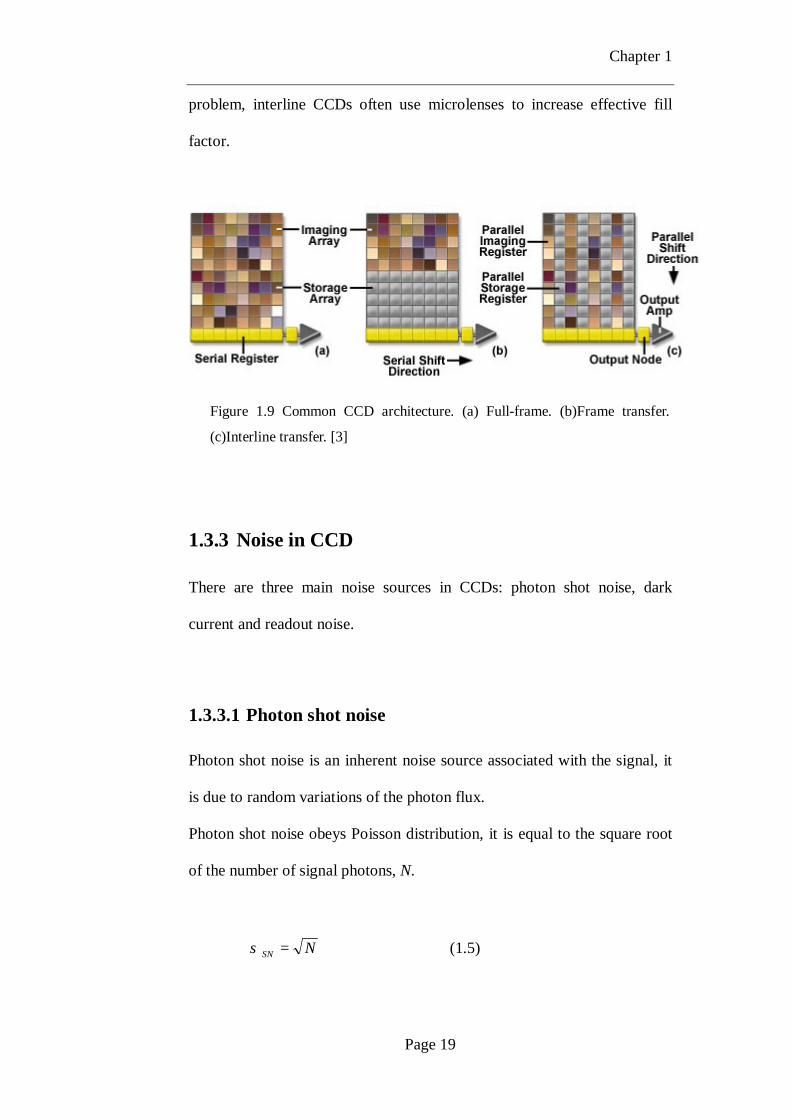
EMCCD is a CCD with a multiplication register which is placed between
the shift register and the output amplifier. Most EMCCDs utilize a frame
transfer CCD structure shown in figure 1.10. The multiplication register
contains several hundreds of elements, and it is clocked at a higher than
usual voltage. This causes 'impact ionization' as the charge is transferred
(Figure 1.11). Impact ionization occurs when a charge has sufficient energy
to create another electron-hole pair and hence a free electron charge in the
conduction band can create another charge. Hence amplification occurs,
and each element of multiplication register acts as an amplifier.
Figure 1.10 EMCCD structure schema. [5]
Chapter 1
Page 23
The gain at each element of the multiplication register is very small (gain
probability P < 2%), but as the number of elements is large (N > 500), the
cumulative effect of many elements allows very high gain (g = (1 + P)N).
As each image electron is amplified to several hundred or thousand before
it is read out by the output amplifier, readout noise is effectively eliminated.
1.4.2 Noise in EMCCD
Most EMCCDs are deeply cooled when operating so the dark current can
be neglected, and the readout noise is overcome by electron multiplication.
However, the EMCCD has some types of noise which normal CCD does
not have.
Figure 1.11 ‘Impact ionization’ in
EMCCD multiplication register. [5]

Chapter 1
Page 24
1.4.2.1 Noise Factor
For a given gain setting there are fluctuations in the actual gain obtained,
because the gain that is applied in the gain register is stochastic. However,
the probability distribution of output charges for a given input charge can
be calculated.
Figure 1.12 is a plot of the probability of output charge for various input
charges for a typical EM gain set to 500. As shown in the figure, if an
output signal of 1,000 electrons is obtained, there is a reasonable
probability that this signal could have resulted from either an input signal
of 1, 2, 3, 4 or even 5 electrons.
However, at very low light levels when there is less than 1 electron falling
on a pixel in a single exposure on average, it can be assumed that a pixel
either contains an electron or not. In this case EMCCD can be used in
Figure 1.12 Probability of EMCCD output charge. [5]

Chapter 1
Page 25
photon counting mode, in this mode a threshold is set above the ordinary
amplifier readout and all events are counted as single photons. This
removes the noise associated with the stochastic multiplication at the cost
of counting multiple electrons in the same pixel as a single electron.
1.4.2.2 Spurious noise (or Clock Induced Charge)
The Spurious Noise or Clock Induced Charge (CIC) is created when charge
is shifted pixel to pixel towards the output amplifier in CCD. There is a
very small but finite probability that charges can knock off additional
charges by impact ionization during charge shift. These unwanted charges
become an additional noise component.
In a normal CCD the noise component is so low and it typically is hidden
by the readout noise or dark current. In an EMCCD however, spurious
charges that occur in the image section are amplified by the EMCCD gain
register and therefore are very detectable. Thus it is essential to minimize
spurious charges in very low light imaging applications such as photon
counting.
1.5 TIRF
Total internal reflection fluorescence microscopy (TIRF) excite fluorescent
probes very near the substrate (within ≤ 100nm). When light travel from a
higher refractive index medium (for example, glass) to a lower refractive

Chapter 1
Page 26
index medium (for example, water), the light is totally reflected by the
interface if incident angle is greater than the critical angle. An
exponentially decaying electromagnetic field called an ‘Evanescent Wave’
is created in the lower refractive index medium and propagates parallel to
the interface. The intensity of the evanescent wave exponentially decays
with perpendicular distance from the interface, it typically penetrates
between 50nm and 200nm into the lower refractive index medium, the
depth depends on media refractive indices, incident angle, and wavelength.
Because the evanescent wave selectively illuminates a very thin layer of
region direct above the substrate, TIRF can provide very high contrast
images of cell membrane with very low background fluorescence
compared with conventional fluorescence microscopy. The TIRF technique
has been used widely in different application, including studies of the
topography of cell–substrate contacts [6,7,8]; measuring dynamics [9] or
self-association [10] of proteins at membranes; and imaging of endocytosis
or exocytosis [11,12].
There are two main types of optical configuration for TIR, prism based and
prismless configuration [13]. In prismless configuration, a high numerical
aperture microscope objective is used for both TIR illumination and
emission observation. While prism based configuration use a prism to
direct the light toward the TIR interface with a separate objective for
emission observation. (Figure 1.13)

Chapter 1
Page 27
In prismless TIRF configuration, evanescent wave illumination is achieved
by focusing a laser beam to a point at the back focal plane (BFP) of the
objective lens. Thus the light emerges from the objective in a collimated
form, which ensures that all the rays are incident on the sample at the same
angle with respect to the optical axis. The point of focus in the back focal
plane is adjusted to be off-axis. At a sufficiently high off-axis radial
distance, the critical angle for TIR can be exceeded and evanescent wave is
created on the interface. The beam can emerge into the immersion oil
(refractive index noil, shown in figure 1.14) at a maximum possible angle
θm measured from the optical axis) given by:
NA= noil sinθm (1.8)
According to Snell’s Law, n sinθ is conserved when the beam traverses
through planar interfaces from one medium to the next, so we have:
noil sinθm = n2 sinθ2 (1.9)
Figure 1.13 Prism based and prismless configuration of TIRF. [14]

Chapter 1
Page 28
(Where subscript 2 refers to coverslip substrate on which the cells grow).
In practical condition the refractive index noil and n2 are usually very close.
For total internal reflection to occur at the interface with an aqueous
medium of refractive index n1, θ2 must be greater than the critical angle θc
as calculated from:
n1 = n2 sinθc (1.10)
From the three equations above, it is obvious that the NA of objective lens
must be greater than n1 (refractive index of aqueous medium) for prismless
TIR configuration. Since n1=1.33 for water, and 1.37 for typical cell
cytoplasm, a high numerical aperture (NA>1.4) microscope objective is
required for this configuration.
Figure 1.14 High NA objective is needed for prismless TIRF
configuration.

Chapter 2
Page 29
Chapter 2 Measurement system and
EMCCD camera optimization
The EMCCD camera used in the project is iXon DV-885KSC-VP (Andor
Technologies, Belfast, UK.), which is a 14 bit cooled EMCCD. The
resolution of the camera is 1004*1002, with 8μm*8μm pixel size. The
camera can be cooled down to -70 degrees when operating and has a
maximum QE of about 65% at 600nm wavelength. More detailed
specification of this camera can be found on [15]. Although the
manufacturer claims that this camera has photon counting sensitivity, it is
necessary to assess the camera performance and confirm whether the
camera really has the capability of photon counting before the
measurement of point spread function.
2.1 Measurement system configuration
To evaluate the performance of the camera, a simple system is built as
figure 2.1.

Chapter 2
Page 30
A 633nm HeNe laser (Power: 20mW, Model: 1135P, JDS Uniphase, CA,
USA) is used as light source in the system. The laser beam is expanded by
two beam expanders. The first beam expander has a magnification of 10
(LINOS Photonics GmbH & Co. KG, Munich, Germany.), the second one
is formed by lens L1 (f=30mm) and L2 (400mm) and the magnification is
13.3. The total magnification is therefore 133 with two beam expander
combined.
As the laser profile has a Gaussian distribution, a small central area of the
laser beam can be considered as approximately an even distribution after
large beam expansion. So we expect to obtain a small area of even
illumination (approx 1cm*1cm, the size of EMCCD chip) which can be
imaged by the EMCCD camera through the iris stop. Because laser is a
coherent source, there are many fringes on the image of expanded beam,
and a laser beam profiler (LBP-2-USB, Newport Corporation, CA USA.) is
Figure 2.1 schematic diagram of measurement system. Laser source is attenuated by
three ND filters, and then expanded by two beam expander with a total 133x
magnification.

Chapter 2
Page 31
used to find the most evenly illuminated area (figure 2.2). Once the area
was determined, the position of the iris stop could be fixed.
In photon counting, even very weak stray light will affect the measurement
dramatically, thus the system must be shielded from stray light by blackout
material. Since the camera has a build-in shutter, the EMCCD is totally
dark when shutter is closed, the stray light shield can be verified by
comparing images taken with shutter opened and closed when laser is off.
To verify the shielding, the EM gain is set to 200 and exposure time is 1
second, at this setting even an extremely faint light signal will be amplified.
Images are taken with shutter opened and closed, we could not observe any
difference between the images even we applied statistical analysis such as
mean and standard deviation, thus the shielding is confirmed to work well.

Chapter 2
Page 32
Three neutral density (ND) filters is used in the system (table 2.1), they can
be combined to generate different attenuation factor. The intensity of
expanded laser beam and actual attenuation factor of neutral density filters
is measured by a power meter (FieldMaxII, Coherent Inc., CA USA.).
Power of expanded laser beam to be imaged by EMCCD (without ND filter
attenuation): 0.3mW/cm2.
Figure 2.2 Software of laser beam profiler showing the central area profile of
expanded laser beam. The image on the left is the beam profile, and the black
curves on the right are vertical and horizontal sum profile, each point on the
curves represents the sum of the row (or column) pixels at corresponding position.
The horizontal profile is almost flat at central area, which means that area is
evenly illuminated. Although there are some fringes, the overall intensity can be
considered to be approximately evenly distributed. Because of the shape of the
beam on the image (the beam profile is not ‘chopped’ at the left and right edge of
the image), the vertical profile curve is not flat. The red curves are ideal Gaussian
distribution given by the software just for reference.

Chapter 2
Page 33
ND1 ND2 ND3
Attenuation factor 77.0 270.4 1936.3
The energy of one photon is given by
λhchfE == (2.1)
Where h is Planck constant (6.626*10-34 Js), f is light frequency, c is light
speed, λ is wave length (633nm in this experiment).
The light beam power measured by power meter is 0.3mW/cm2, and the
size of pixel on the EMCCD is 8μm by 8μm, thus the photon number on
each pixel can be calculated.
According to calculation, the attenuation of three neutral density filters,
give a light flux arrived at the camera 15.17 photon/pixel/second, take
account of the QE of 60%, the effective photon number is 9.10
photon/pixel/second (approximate 9 photon/pixel/second).
2.2 Camera optimization and EM gain calibration
Table 2.1 Attenuation factor of three neutral density filters.

Chapter 2
Page 34
2.2.1 Camera optimization
The image acquisition and camera control software is iQ version 1.5
(Andor technologies.), which provide some adjustable parameters of the
camera (figure 2.3).
Horizontal readout time determines the collected charge moving speed
from horizontal shift register into the output node of the amplifier. As the
faster the readout speed the more readout noise is created, this horizontal
readout time is set to 13 MHz to keep readout noise low, although a faster
speed of 35 MHz is also provided by the camera.
Figure 2.3 Camera setting parameters.

Chapter 2
Page 35
At present time all EMCCDs are of Frame Transfer architecture and
require a vertical shift of the image into a storage CCD area prior to
readout. The speed and voltage applied during this vertical shift is closely
related to CIC level and thus can significantly affect the quality of the
image and the background noise level.
According to the manual of the camera, a faster vertical shift leads to lower
background or clock induced charge (CIC) and therefore lower noise.
However, faster shift can also lead to lower charge transfer efficiency,
which may cause a residual smeared image on the image area.
To overcome this effect the vertical shift voltage can be increased
(+1,+2,+3 or +4), but increasing the vertical shift voltage can result in
higher CIC level, thus this parameter should be carefully adjusted.
The default settings of theses parameter are: vertical shift speed: 1.9 μs,
vertical shift voltage: normal. To reduce noise level, we tried to change
vertical shift speed to 0.5 μs, and the noise level is slightly decreased.
However, this resulted in smear image and the image quality is
significantly deteriorated, as shown in figure 2.4.

Chapter 2
Page 36
Figure 2.4 Image acquired with different vertical shift speed. (a) Vertical
shift speed: 0.5 μs (smeared image). (b) Vertical shift speed: 1.9 μs (normal
image).
Light flux intensity: 1 photon/pixel/frame, 16 frames averaged. On the
pictures, the image with 0.5 μs vertical shift speed is smear and all the detail
of diffraction fringes is lost.
(b)
(a)

Chapter 2
Page 37
To overcome this problem, we tried to increase vertical shift voltage, but
the noise is increased dramatically when the vertical shift voltage is
increased, even at +1. Thus these parameters are restored to default, to keep
image quality and relatively low noise.
The baseline clamp is another option which may affect the measurement.
According to the manual of the camera, the option ensures that the camera
electronics adjusts automatically to deliver a baseline count (zero light grey
value) at a certain fixed value, so drift in the baseline level caused by small
changes in heat generation of the driving electronics can be prevented.
This option is on by default, but I found this option may result in signal
level shift for weak signal. Figure 2.5. shows the probability distribution of
signal from one pixel with 1 photon/pixel/frame light intensity. As the
photon arrival obeys a Poisson distribution, the probability for no photon
arrival, one photon arrival and more than one photon are approximate 37%,
37% and 26% respectively. Since the camera is not sensitive enough to
detect every ‘one photon arrival’ event, the peak of signal distribution
curve represent the situation that no signal output (i.e. the background), so
the peak position in curves of signal and background should coincide.
However the peak in signal curve is shifted left with baseline clamp on
(figure 2.5 (a)), although the shift is small (about 5-10 count in grey value)
and not very significant, it may have some effect on threshold processing in
photon counting. This shift does not exist with baseline clamp off, as

Chapter 2
Page 38
shown in figure 2.5 (b), thus the option is turned off in the experiment,
although the baseline might drift during experiment with this option off.
(a)

Chapter 2
Page 39
2.2.2 EM gain calibration
The EM gain can be controlled by the software. However, the gain value in
the software is not linearly proportional to the real EM gain of this camera,
although some newer models of EMCCD cameras provide linear gain
setting. Thus gain calibration for the camera is needed. To calibrate EM
gain, an object with constant light intensity is imaged on the camera,
Figure 2.5 Statistical data of signal of one pixel in a series of 1000 images. Light flux
intensity: 1 photon/pixel/frame. (a) Baseline clamp ON. (b) Baseline clamp OFF.
(b)

Chapter 2
Page 40
several pictures are taken at different EM gain settings, and the grey value
subtracted by background is proportional to real gain. As the camera is a 14
bit EMCCD, the grey value on image ranges from 0 to 16383, and the EM
gain can be up to more than 1000, the camera can be saturated at high gain.
Thus exposure time must be reduced at high gain setting, and the exposure
time ratio need to be take into account when calculating real gain.
Software gain Real gain
OFF 1
1 2.4
50 4.5
100 12.1
150 55.4
175 149
185 235
200 481
210 776
220 1308
230 2500
Table 2.2 Relationship between real gain and software gain setting.

Chapter 2
Page 41
2.2.3 Choosing a suitable EM gain value
Although signal is amplified greatly at high EM gain, the noise is also
increased significantly at the same time. The EM gain value need to be
carefully choose to achieve optimized signal to noise ratio. The background
noise is measured by calculating standard deviation of totally dark image of
different gain value. We define the ratio real gain / background standard
deviation as the ‘signal to noise ratio’ in the experiment. The ratio is
calculated for different gain and the most suitable gain value can be
obtained.
Figure 2.6 Plot of software gain setting versus real gain value

Chapter 2
Page 42
Software gain Real gain Background standard deviation Real gain/std dev.
OFF 1 3.6 0.28
1 2.4 3.7 0.65
50 4.5 3.7 1.22
100 12.1 3.8 3.21
150 55.4 6.1 9.07
175 149 12.6 11.8
185 235 20.0 11.7
200 481 41.0 11.7
210 776 68.6 11.3
220 1308 119.1 11.0
Table 2.3 Relationship between software gain and ratio of real gain/background
standard deviation
Figure 2.7 Plot of software gain versus ratio of real gain/background
standard deviation

Chapter 2
Page 43
According to table 2.3 and figure 2.7, at low gain value the ratio ‘real
gain/background standard deviation’ increases rapidly with gain, which
means the gain has significant effect on improving signal to noise ratio.
The ratio reaches its peak at gain 175 and almost keep constant till gain
200, then it began to decrease when gain is greater than 200, which is due
to the dramatically increase of noise, so the effective signal to noise ratio
will not get improvement, or even get worse as gain go beyond 200. Thus
the gain value of 175 is considered as the most suitable gain value for the
experiment.

Chapter 3
Page 44
Chapter 3 Evaluating photon counting
performance of EMCCD
3.1 Principle of photon counting by EMCCD
Since the EM amplification that is applied in the gain register is a
stochastic process, although probability distribution can be calculated
(figure 1.13), the exact input photon number cannot be deduced by the
magnitude of output signal.
To perform photon counting, the light intensity must be kept at a very low
level so it can be assumed that either only one photon, or no photon arrive
at one pixel during one exposure. Under this condition, a threshold is set
and all signals above the threshold will be counted as signal of one photon,
the signals below the threshold will be considered as dark.
The arrival photon number obeys Poisson distribution, which is given by
!exp),(
nnp
n λλλ
−= (3.1)
Where p(n,λ) is the probability of n events occurring when the averages
(expectation number) is λ.
Table 3.1 gives some probability with different λ (mean value).

Chapter 3
Page 45
Mean (λ) 0.05 0.1 0.2 0.5 1 2 5
P(n=0) 0.95123 0.90484 0.81873 0.60653 0.36788 0.135335 0.006738
P(n=1) 0.047561 0.090484 0.16375 0.30327 0.36788 0.270671 0.03369
P(n=2) 0.001189 0.004524 0.016375 0.075816 0.18394 0.270671 0.084224
P(n=3) 1.98E-05 0.000151 0.001092 0.012636 0.061313 0.180447 0.140374
P(n>1) 0.001209 0.004679 0.017523 0.090204 0.26424 0.593994 0.959572
Ratio P(n=1)/P(n>1) 39.336 19.339 9.3446 3.362 1.3922 0.455679 0.035109
As the light intensity measured above is the average intensity, for example
at light flux 1 photon/pixel/exposure, there is still a relative high
probability P(n>1)=0.26424 of having more than one photon in a exposure,
the light intensity should be kept very low to satisfy the condition ‘either
only one photon, or no photon arrives during one exposure’. At light
intensity 0.1 photon/pixel/exposure, the probability of having more than
one photon P(n>1)=0.004679 is very small and can be considered to be
negligible.
3.2 Method
Although the light intensity is measured by power meter, there are some
fringes on the laser beam, and not every pixel illuminated by laser beam
has the same intensity. Since the light intensity measured by the power
meter is the average power over the area, so we need to choose pixels
Table 3.1 Poisson distribution probability with different λ.

Chapter 3
Page 46
having light intensity corresponding to the intensity measured by power
meter.
Firstly ND1 and ND2 are removed so the intensity is high enough for
normal CCD imaging, the EM gain in the camera is also turned off. Then
an image is taken by the camera and the histogram is obtained, as shown in
figure 3.1. The image on figure 3.1(a) has some fringes, the grey value
difference between peak and lowest position is about 15% of the average
value of the entity illuminated area. On figure 3.1(b) the left peak on the
histogram represents dark pixels without illumination, the central
symmetrical distribution represents the pixels illuminated by the laser beam.
The average power of the illuminated area is obtained by the power meter,
which corresponds to the central position of the distribution on the
histogram. The grey value at central position is recorded and the pixels
with the same grey value have the same intensity with average power of the
area.
According to the power meter measurement, the output power of laser is
not perfectly constant, the fluctuation is approximate 5%. The attenuation
factors of ND filters, although calibrated by the power meter, still have an
error of approximate 2~3% each, it is estimated the error is approximately
5% ( 203.03× ) when three ND filters combined. Therefore the total
error of photon number arrival at the camera is approximate 7%
( 22 05.005.0 + ).

Chapter 3
Page 47
After choosing pixels, ND1 and ND2 are restored and EM gain in the
camera is set to 175, the exposure time is set as corresponding required
mean photon number (light intensity). For example, the laser beam
intensity is 9 photon/pixel/second, a exposure time of 111 millisecond is
needed to achieve the intensity of 1 photon/pixel/exposure, and 11
millisecond for 0.1 photon/pixel/exposure and so on. The exposure is set as
repeating up to 50,000 times automatically, so a stack of images can be
Figure 3.1 (a) Image of laser beam without ND1 and ND2. (b) Histogram of
the image.
(a)
(b)

Chapter 3
Page 48
obtained. To save storage space and increase acquisition speed, only a
small area of 80*80 pixels is recorded. For each light intensity level, two
stacks of images are acquired, one with camera shutter opened represents
signal, and one with shutter closed represents background noise.
3.3 Result and data analysis
3.3.1 Probability density distribution
For each pixel chosen previously, the pixel grey value is read from the
image stacks, so a series of grey value data is obtained for one pixel. These
data is processed by statistical analysis, and the mean, standard deviation
and probability distribution are obtained. Table 3.2 shows the statistical
data of a pixel signal, for light intensity 0.1 and 0.2 photon/pixel/exposure,
50,000 exposures are acquired, and for light intensity 1
photon/pixel/exposure, 10,000 exposures are acquired. Figure 3.2, 3.3 and
3.4 shows the probability density distribution (probability density function,
PDF) of the pixel signal response with different illumination light intensity.

Chapter 3
Page 49
Light intensity (photon/pixel/exposure) 0.1 0.2 1
Signal mean 879.15 876.24 886.4
Background mean 876.63 873.81 872.08
Signal std. deviation 16.965 19.012 32.622
Background std. deviation 13.324 13.624 13.791
Figure 3.2 Probability density distribution of one pixel signal from a series
of 50,000 images, illumination light intensity 0.1 photon/pixel/exposure.
Table 3.2 Mean and standard deviation of signal and background at
different light intensity.

Chapter 3
Page 50
Figure 3.3 Probability density distribution of one pixel signal from a series of
50,000 images, illumination light intensity 0.2 photon/pixel/exposure.
Figure 3.4 Probability density distribution of one pixel signal from a series of
10,000 images, illumination light intensity 1 photon/pixel/exposure.

Chapter 3
Page 51
According to the figures above, the signal and background distribution is
very close at intensity 0.1 or 0.2 photon/pixel/exposure, it is because most
exposures are dark at low intensity, for example, at intensity 0.1
photon/pixel/exposure approximately 10% of total exposures receive a
photon, and 90% exposures are dark without photon.
At intensity 1 photon/pixel/exposure the signal and background distribution
are more separated, the signal has higher probability at high grey value.
However, according Poisson distribution, at this intensity the probability of
having more than one photon arrival during one exposure is about 26.4%,
and if photon counting is performed at this intensity, all situations with
more than one photon will be counted as one photon.
The background distribution has a peak (around grey value 870), which
represents the baseline (zero light grey value) of the camera. The
background probability decrease dramatically as grey value increases, but
it does not drop to zero immediately, above grey value 880~890 the
probability decreases more slowly and can spread widely up to around
1000. Thus the distribution of background and signal overlap, this
overlapping causes a problem on photon counting. As described previously
a threshold is needed in photon counting, the widespread distribution of
background make it difficult to set the value of threshold. If the threshold is
set low, the noise or false counting will be very high, on the other hand, if
the threshold is set as high, the noise can be eliminated but most signal is
excluded at the same time. This problem is especially significant at low

Chapter 3
Page 52
light intensity, as the distribution of signal and background are very close,
unfortunately the photon counting requires low light intensity to satisfy the
condition ‘no more than one photon arrives during one exposure’. Thus the
background noise level of the EMCCD camera determines whether photon
counting is feasible.
3.3.2 Cumulative distribution
To research the performance of the camera, a cumulative distribution
function (CDF) is calculated from corresponding probability density
distribution. The cumulative distribution function is obtained by setting a
variable ‘value' and calculating the probability that x≥ 'value' from
probability density distribution, and this probability is plot against 'value'.

Chapter 3
Page 53
Figure 3.5 Cumulative distribution function of one pixel signal from a series
of 50,000 images, illumination light intensity 0.1 photon/pixel/exposure.
Figure 3.6 Cumulative distribution function of one pixel signal from a series
of 50,000 images, illumination light intensity 0.2 photon/pixel/exposure.

Chapter 3
Page 54
The cumulative distribution functions give the probability that signal or
background is greater than a certain threshold value at different photon
mean number, so the proper threshold value can be determined from these
cumulative distribution functions.
At low light intensity, the probability that of signal does not exceed that of
background too much no matter what threshold value is chosen (figure 3.5
and 3.6), which is caused by the widely spread distribution of background
and the overlap of background and signal distribution as described above.
As a result, the signal to noise ratio is low at low light intensity. For
example, at intensity 0.1 photon/pixel/exposure, if value 900 is chosen as
Figure 3.7 Cumulative distribution function of one pixel signal from a series
of 50,000 images, illumination light intensity 1 photon/pixel/exposure.

Chapter 3
Page 55
threshold, the probability of signal is about 0.067, and probability of
background is about 0.041. As the signal obtained from camera also
includes background noise, more than half of the counts will be noise if
photon counting is performed at this intensity with threshold value 900.
At higher light intensity, the probability of signal and background are
better separated (figure 3.7) so the signal to noise ratio is higher. On the
figure, the ratio ‘signal : background’ could be higher if the threshold is set
at a higher value, as the background is reduced to very low, however it is
not feasible in practice.
If the threshold is set too high, most signals will be excluded and only
strong signals can remain, since the arrival of a photon obeys the Poisson
distribution, at intensity 1 photon/pixel/exposure there is still a non-
negligible probability of more than one photon (about 26.4%). According
to probability distribution of EMCCD output charge (figure 1.13), the more
input electron the higher probability of having a larger number output
charge and therefore a stronger signal. In this case, the signals remained
after threshold processing is more likely to be due to the situation of two or
more photons rather than one, so the signal might not represent one photon
and it could result in error in photon counting. Moreover, since most
signals are excluded after threshold processing, the effective detection
efficiency will be very low, so more exposures are needed to acquire
enough signals, and more acquisition time and storage space is needed.

Chapter 3
Page 56
3.3.3 Estimation of the CDF of one photon
According to table 3.1, at mean 0.1, the probability P(n>1) is very small so
it can be neglected, so P(n=1) can be approximated by P(n>0), thus P(n=0)
and P(n=1) are approximate 0.905 and 0.095 respectively. The CDF(0.1) in
figure 4.5 can be considered as:
)1(095.0)0(905.0)1.0( CDFCDFCDF += (3.2)
Where CDF(0.1) is it is the CDF of signal in figure 3.5, CDF(0) is
cumulative distribution function of pixel signal when there is no photon
incident, it is the CDF of background in figure 3.5. CDF(1) is cumulative
distribution function of pixel signal when there is one and only one photon
incident, it can be calculated from equation 3.2. Figure 3.8 shows the
calculated CDF(1) from figure 3.5.

Chapter 3
Page 57
The calculated CDF(1) in figure 3.8 has some peaks near value 870 where
the curve of signal and background are steep. The curve of CDF should not
have peaks in real situation, as the cumulative distribution function is
always monotonically decrease by its definition, peaks in CDF means
negative probability in the regions which is not possible in real world. The
peak in the calculated CDF(1) is possibly due to measurement error, a very
small different between signal and background in the steep region will be
significant, since the option baseline clamp is off, the baseline level might
drift slightly during the experiment, which might result in the peaks in the
curve. Therefore the data in the steep region is not reliable and will not be
Figure 3.8, Curve of calculated CDF(1) of the pixel on figure 4.5 by
( ) 095.0/)0(905.0)1.0( CDFCDF − . The CDF of signal and
background (black solid and black dashed line) are same as that in figure
3.5.

Chapter 3
Page 58
used. Table 3.2 shows the probability of signal of 1 photon and background
at several different threshold values.
Threshold value Background probability
Signal of 1 photon probability
882 9.33% 53.04%
894 5.03% 34.57%
942 0.99% 8.86%
963 0.5% 4.58%
3.3.4 Simulation of signal distribution
The signal and background distribution can be calculated by a simulation
model. Let the probability of detecting a photon when it is actually there
be dp , the probability of a false positive (the signal when there is no photon)
be fp . The expected photon number at the pixel is f, where the number f
should be much less than 1, and a total image number of N is taken in the
measurement.
Thus within a single frame the probability of detecting a photon when it is
actually present is:
( ) dd pfpp )0,(1' −= (3.3)
Table 3.2 Probability value of CDF(0) and CDF(1) in figure 3.8 at different
threshold value.

Chapter 3
Page 59
Where the function ),( bap is the Poisson function for expectation value a
and value b, the number f should be much less than 1, so P(n=1) can be
approximated by P(n>0).
The probability of false positive:
ff pfpp )0,('= (3.4)
The probability of detector output p will be 'fp when it is in totally dark.
If there is photon incident, the total signal probability of detector output
with background will be
'' fd ppp += (3.5)
So the distribution can be calculated by Binomial distribution for different
values of dp , fp , f and N. For example using data %57.34=dp ,
%03.5=fp in table 3.2, the signal and background probability
distributions at different f and N are obtained by MATLAB simulation in
figure 3.9 and 3.10.

Chapter 3
Page 60
Image number N Expectation photon number f=0.1
50,000
10,000
3,000

Chapter 3
Page 61
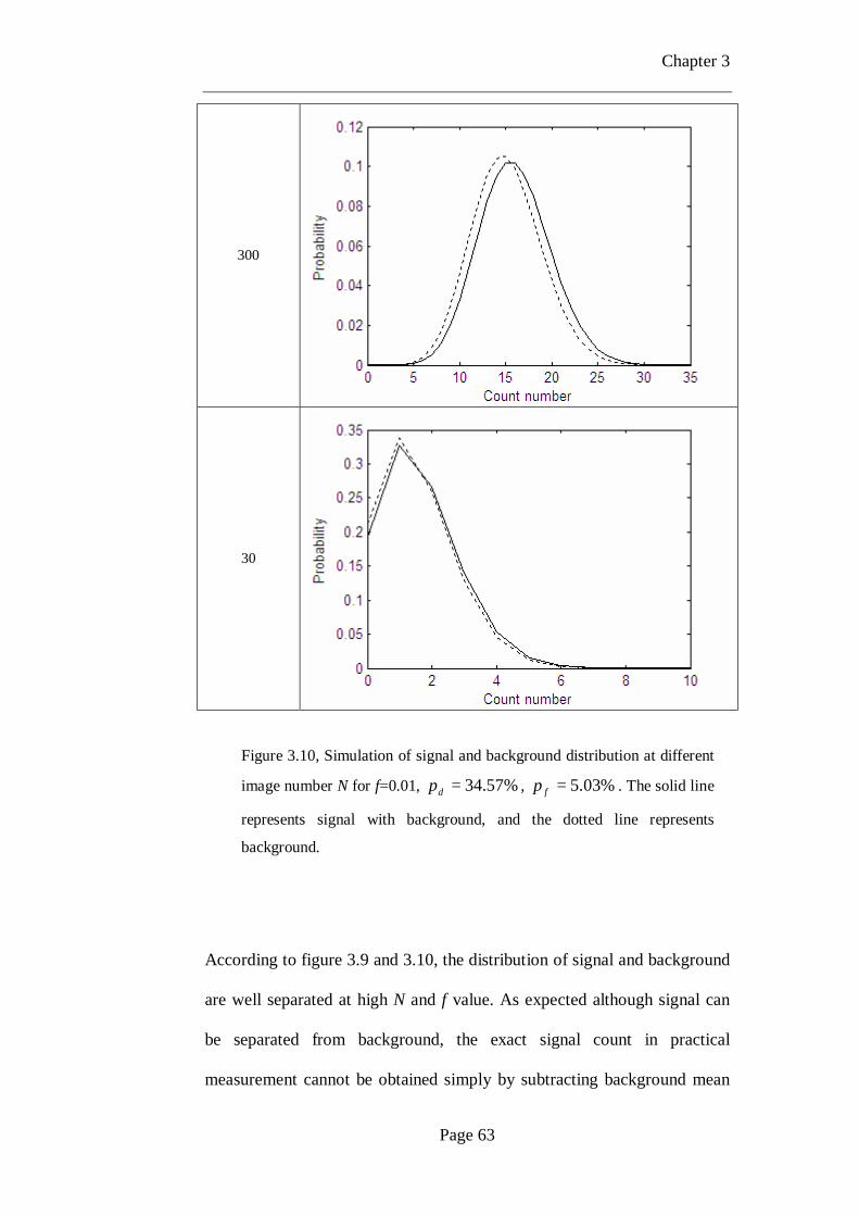
300
30
Figure 3.9, Simulation of signal and background distribution at different
image number N for f=0.1, %57.34=dp , %03.5=fp . The solid line
represents signal with background, and the dotted line represents
background.

Chapter 3
Page 62
Image number N Expectation photon number f=0.01
50,000
10,000
3,000
Chapter 3
Page 63
300
30
According to figure 3.9 and 3.10, the distribution of signal and background
are well separated at high N and f value. As expected although signal can
be separated from background, the exact signal count in practical
measurement cannot be obtained simply by subtracting background mean
Figure 3.10, Simulation of signal and background distribution at different
image number N for f=0.01, %57.34=dp , %03.5=fp . The solid line
represents signal with background, and the dotted line represents
background.

Chapter 3
Page 64
value from signal, because the background noise is distributed in a region
and the exact noise included in the output signal is unknown.
The distributions become closer and overlap when N decrease, for example,
at f=0.1, the distributions begin to overlap when N is less than 3000. At
N=30, where the total expectation photon number is approximate 1
( 0371.130%57.341.0 =×× ), most of the two distributions overlap and it is
very difficult to distinguish signal from background under this condition.
Therefore the camera might not be ideal for photon counting.
The distributions also become closer and overlap with the decrease of f
number, it can be observed that at f=0.01 the distribution overlap even at
N=50,000. At the same total expectation photon number, the distribution
with lower f number is more overlapped than that of higher f number, as
shown in figure 3.11. Thus it is more difficult for the camera to distinguish
signal from background at lower light level.

Chapter 3
Page 65
f=0.1, N=300 f=0.01, N=3,000
f=0.1, N=30 f=0.01, N=300
For a point spread function which can be described by a jinc function, the
intensity profile is the square of jinc function, and the intensity of first
sidelobe is only approximate 1.75% of the peak intensity. According to the
simulation result, it will be almost impossible to distinguish sidelobe of
point spread function in photon counting with the parameters used for the
present camera.
Figure 3.11 Comparison of distribution at different expected photon
number f under the same total expectation photon number. The solid line
represents signal with background, and the dotted line represents
background.
Chapter 3
Page 66
3.3.5 Conclusion
According to the experiment data and simulation result above, although the
camera is able to separate signal from background when expectation
photon number f and image number N is relative high (for example, f=0.1
and N=10,000), the exact signal count cannot be obtained because of the
variance of background.
When the expectation photon number f decreases, the situation become
worse, the distributions of signal and background overlap. Thus the region
of point spread function with lower intensity (for example, the sidelobe of
PSF) will be merged by background and cannot be detected.
The value dp and fp determines the performance of the detector, for an
ideal detector 1=dp and 0=fp . However the practical detector cannot be
so good, for example the practical value %57.34=dp , %03.5=fp are
used in the simulation above. The value of fp can also be calculated for a
‘good performance’ detector, for example, under the
condition %57.34=dp , f=0.1, N=30 where the total expectation photon
number is approximate 1, fp need to be less than approximate 0.2% to well
separate signal and background (figure 3.12). It can also be observed that
to achieve a good performance at a lower f number, an even lower fp is
needed.

Chapter 3
Page 67
The camera used in the experiment has a relative high value of fp , thus it
is not very ideal for photon counting.
Figure 3.12, Simulation of signal and background distribution at image
number N=30, f=0.1, %57.34=dp , %2.0=fp , the total expectation
photon number is approximate 1. The solid line represents signal with
background, and the dotted line represents background.
At count number=1 the background probability is 0.057, while the signal
probability is 0.37. The background probability is very small and
negligible when count number is greater than 2, thus it can be considered
to be ‘good performance’ under this condition.
Chapter 4
Page 68
Chapter 4 Photon counting with
flourophore in TIRF
Although the performance of the camera is not ideal, attempt is still made
to perform photon counting with fluorescent beads in TIRF.
4.1 Instrument configuration
The instrument system is TIRF and TIRM combined [16], but only TIRF is
used in this experiment. The TIR system employs prismless configuration.
A Meiji (Axbridge, Somerset, UK) TC5400 inverted biological microscope
with a high-NA objective lens (Zeiss Plan-Fluar 100 × 1.45 NA) (Carl
Zeiss Ltd., Welwyn Garden City, Hertfordshire, UK) formed the central
component of the system, while a 488nm solid state laser (20mW, Protera
488-15, Novalux, Sunnyvale, CA) or a 532nm solid state laser (50mW,
BWN 532-50, B&W TEK, Newark, DE) is used for TIRF light source.
Figure 4.1 shows the set-up of the system, L1-L2 and L3-L4 are used to
expand the laser beam so a field of approximately 200μm2 can be
illuminated on the object plane. L1 equals L3 and L2 equals L4, the focal
length of L1 and L3 is 12mm and focal length of L2 and L4 is 250mm, thus
the magnification is approximately 21X.

Chapter 4
Page 69
For the dual-colour TIRF illumination, 488nm and 532nm laser beam are
combined at a dichroic beamsplitter DBS. The mirror and focusing lens L5
can be translated by the stage, so the position of the focal point in the back
focal plane (BFP) of the microscope objective lens can be moved, therefore
the incident illumination angle can be changed. Fluorescent emission and
reflected LED illumination pass through the multi-band dichroic
beamsplitter MDBS, and tube lens L10 forms an image on the EMCCD.
For 532nm excitation wavelength, the emission fluorescent wavelength is
around 560nm, which is near the peak QE wavelength of the EMCCD, thus
532nm laser is used in the experiment. The sample is fluorescent beads of
170nm in size (540/560nm, Catalog Number: P7220, Molecular Probes,
Inc.) The camera is connected to microscope via a 2.5X adapter (Meiji
Techno UK Ltd.) and the magnification on the camera is approximate
250X. According to equation 1.2, with NA 1.45 and wavelength 560nm,
the width of PSF is about 470nm, however since the size of beads (170nm)
is not much smaller than width of PSF (470nm), the actual image size of
the beads is the convolution of bead with PSF, and the image will be a little
wider than 470nm. With magnification of 250X, length of 470nm on
objective plane will be 117.5μm on CCD and occupy about 15 pixels (pixel
size: 8μm).

Chapter 4
Page 70
4.2 Method
The solution of fluorescent beads is diluted 1000 times before use. A
droplet of solution is placed on a glass cover slip, then wait until the
solution dry so the fluorescent beads are immobilized on the coverslip. A
50% ND filter is placed in front of laser so the emission light of fluorescent
beads is strong enough for eyepiece observation and camera imaging
without EM gain. Figure 4.2 shows an image of a fluorescent bead in this
condition, the shape of point spread function is clear and some diffraction
fringes are also visible. The positions of pixels with peak intensity of
fluorescent bead image are recorded, and these pixels will be used for
signal statistic in photon counting later on.
Figure 4.1 Schematic diagram of TIRF & TIRM combined system.

Chapter 4
Page 71
After locating and focusing, another ND filter with attenuation factor of
approximate 2000 is inserted and the EM gain of camera is turned on to
perform photon counting.
The image acquisition of photon counting is almost the same as described
previously, a small region (ROI, region of interest) containing one bead is
selected, the camera is set to repeat exposure many times automatically (up
to 10,000 times), and stacks of images are acquired. However since the
emission intensity of beads is unknown, several exposure time are used so
the mean intensity can be estimated. For each exposure time, two stacks of
images are acquired, one for signal and one for background.
Baseline stability
In previous experiment with laser beam illuminating CCD, the option
baseline clamp will result in signal shift (figure 2.5), thus the option was
Figure 4.2 Image of a fluorescent bead under high intensity excitation
beam. EM gain of camera is turned off. (b) is (a) with increased
brightness to show sidelobe of the image.
(b) (a)

Chapter 4
Page 72
turned off in that experiment. However the baseline stability is important
for threshold processing and the drift of baseline will cause error. To
determine whether the option baseline clamp is suitable for TIRF, an
experiment is made to compare the result of imaging fluorescent bead with
baseline clamp on and off.
Figure 4.3 (a)

Chapter 4
Page 73
Figure 4.3 shows the signal distribution with option baseline clamp on and
off, unlike figure 2.5, there is no difference between the two results. The
signal distribution shift in figure 2.5 is probably because that all area of
image is illuminated in previous experiment, while there is only a small
area is illuminated in the fluorescent bead image, and perhaps the function
baseline clamp needs a reference background to work properly. Since the
option baseline clamp will not cause signal shift in TIRF, it is turned on in
this experiment.
Figure 4.3 Statistical distribution of signal of one pixel with peak intensity of
fluorescent bead, signal is extracted from a serial of 1000 images. Exposure time 100
ms. (a) Baseline clamp ON. (b) Baseline clamp OFF.
Figure 4.3 (b)

Chapter 4
Page 74
4.3 Analysis of results
After the images are acquired, the signals of peak intensity pixels are
extracted from image stack. Table 4.1 shows the statistical data of a pixel
signal.
Exposure time (ms) 10 50 100
Signal mean 1005.97 1008.98 1017.81
Background mean 1004.58 1003.59 1004.73
Signal std. deviation 14.36 20.04 29.37
Background std. deviation 10.96 12.21 13.54
According to table 4.1, the difference between signal mean and background
mean at 100 ms exposure time is very close to that of light intensity 1
photon/pixel/exposure (Table 3.2), thus it is estimated that the light
intensity on the pixel is approximate 1 photon/pixel/exposure at 100 ms
exposure time, and 0.1 photon/pixel/exposure at 10 ms exposure time.
Light intensity of 0.1 photon/pixel/exposure is low enough for photon
counting, so cumulative distribution function (CDF) of the pixel signal at
10ms exposure time is plotted for threshold value determination. Figure 4.4
shows the CDF, the probabilities of signal and background at various
threshold values can be obtained from this CDF, and some probabilities are
given in table 4.2.
Table 4.1 Mean and standard deviation of signal and background of one
pixel at different exposure time.

Chapter 4
Page 75
Figure 4.4 Cumulative distribution function of signal of a pixel with
fluorescent bead peak intensity. Signal is extracted from a serial of 10,000
images, exposure time 10 ms.

Chapter 4
Page 76
Background probability Threshold value Signal probability
10% 1010 13.06%
5% 1020 7.38%
1% 1059 1.6%
0.5% 1078 0.81%
To compare the results of different threshold value, three threshold values
1010, 1020 and 1059 are chosen for threshold processing. The threshold
processing is simple, the image is analysed and all pixels with grey value
higher than the threshold value are set to ‘1’ and the other pixels are set to
‘0’, thus the image is converted to a binary image. This step is applied to
all images in the stack, so all 10,000 images are converted to binary image,
then all these 10,000 images are summed up to form a final image.
Table 4.2 Probability of background and signal at different threshold value.

Chapter 4
Page 77
(a)
(b)
(c)
Figure 4.5 Resultant image of threshold processing at different threshold value.
Threshold value: (a) 1010; (b) 1020; (c) 1059.
Plot on the right is line profile of the dotted line on the corresponding left image.

Chapter 4
Page 78
The resultant images of threshold processing at various threshold values
are shown in figure 4.5, the shape of fluorescent bead can be observed in
the images, but the background is noisy, and the sidelobe cannot be
detected, as predicted in previous simulation. The background in the
images is due to the noise in EMCCD, the noise results in ‘false positive’
or ‘false count’ where there is no photon incident. The actual photon signal
cannot be obtained by simply subtracting the background, because the
background is not uniform and varies from pixel to pixel.
Although the background in the images is not uniform, it can be observed
from the line profile of figure 4.5 that the background level fluctuates
around a certain value which equals the product of background probability
at corresponding threshold value (table 4.2) and total image number in the
stack.
To study the variance of background in resultant image, the stack of 10,000
images for background (acquired in totally dark) is threshold processed,
then the mean and standard deviation of the resultant image are calculated,
as shown in table 4.3. According to the data in table 4.3, the mean and
variance of resultant background image is very close, thus it can be
assumed that the background noise obeys Poisson distribution.

Chapter 4
Page 79
Threshold value Mean Standard deviation (σ) Variance (σ2)
1010 991.23 32.44 1052.35
1020 511.44 22.51 506.70
1059 110.50 10.42 108.58
At a certain threshold value, let the probability of signal on a pixel be p, the
probability of background on the same pixel be q, and the total image
number in the stack is N. The mean value of signal count will be p*N, and
the mean value of background count will be q*N. According to the
assumption above, the background obeys Poisson distribution, and the
standard deviation of background is Nq * . The actual photon signal is
unknown, but it can be approximated by (p-q)*N, the difference between
mean of signal and background. Thus the signal to noise ratio on resultant
image of threshold processing can be express as:
( ) Nqqp
qNNqpSNR −
=−
= (4.1)
It is obvious that the larger N, the higher SNR, and the coefficient qqp − of
the pixel on figure 4.4 can be calculated and plotted on figure 4.6. In figure
4.6, the coefficient is maximum (approximate 0.1) when threshold value is
between 1010 and 1030, and the coefficient decreases as the threshold
Table 4.3 Statistical data of background image after threshold processing at
variant threshold value.

Chapter 4
Page 80
value increases. The coefficient is meaningless as threshold value is above
1100, because the probability of signal and background are almost zero.
Figure 4.6 (a)

Chapter 4
Page 81
According to figure 4.6, the maximum coefficient value is approximate 0.1,
for a stack of 10,000 images, the SNR is approximate 10, which is not a
very low value. The greater the number of images, the more total photon
signal count in resultant image, although the actual total photon signal
count is unknown, it can be estimated by subtracting background mean
value from signal. It is estimated that the total photon signal count in
resultant image is approximate 25,000 at threshold value 1020 and
approximate 50,000 at threshold value 1010.
Figure 4.6 Curve of coefficient qqp −
of the pixel on figure 4.4. The
CDF of signal and background (blue and red line) are same as that in
figure 4.4. (b) is an enlarged area in (a) to show detail of curve.
Figure 4.6 (b)

Chapter 4
Page 82
However, if a smaller number of photons, for example several hundred to
one thousand photons in each image, is required in Monte Carlo method,
this requires much smaller number of image, and results in lower SNR. For
example, at threshold value 1020, the number of image will be 400 if a
resultant image with only 1,000 photon counts is needed, and the SNR of
peak intensity in the image will be 2400*1.0 = , this SNR is too low and
can result in significant error. At this point of view, the noise in the camera
is main problem in photon counting, so my conclusion is that the camera is
not ideal for photon counting and STF measurement cannot be performed
with this camera.
Moreover, the total time of image acquisition will be long under this
condition. Leaving alone the SNR problem, a resultant image with 1,000
photon counts requires 400 exposures as described above, and tens of
thousands of such resultant images are needed in Monte Carlo method. For
example, to obtain 5,000 resultant images, 2,000,000 exposures are
required. The camera needs approximate 4 minutes to complete 10,000
exposures, thus the total time for 2,000,000 exposures will be 800 minutes,
or 13.3 hours. During such a long time, the fluorescent beads might suffer
photobleaching, although the fluorescent beads are excited at very low
intensity.
Chapter 5
Page 83
Chapter 5 Conclusion
5.1 Summary and conclusion
In this project, attempt is made to perform photon counting which can be
use to measure stochastic transfer function (STF) by Monte Carlo method.
In the Monte Carlo method, images of a point source containing only
several hundred or thousands photons are required, a large number of such
images are collected and Fourier transformed, and the mean and variance
of distribution at each spatial frequency of the imaging system can be
recovered, thus the STF can be obtained.
An EMCCD camera, which is supposed to have photon counting sensitivity,
is used as photon counting device in the experiment. However, although it
has been optimized, the EMCCD camera is found to be not as sensitive as
the manufacturer claimed during the experiment, and an experiment is
carried out to evaluate the performance of the EMCCD camera. In the
evaluation experiment, the camera is illuminated by a beam of laser with
known intensity (very weak intensity, 0.1 photon/exposure/pixel for
example) and the output signal and background noise of the camera is
recorded and statistical data is obtained. Moreover, a simulation based on
the experiment data gives the EMCCD output signal distribution under
different conditions.

Chapter 5
Page 84
According to the experimental data and simulation results, the EMCCD
camera cannot separate signal from background at low light intensity
because of its background noise, thus it is turned out to be not suitable for
photon counting.
Moreover, an experiment of photon counting in TIRF with fluorescent
beads in which condition the practical STF measurement will be performed
is also carried out. According to the experiment result, the EMCCD is able
to separate signal from background at high light intensity, but unable to
separate at low intensity, which match the prediction of the simulation.
Therefore the conclusion about the EMCCD camera used in this project is
that it is not capable of performing photon counting for the Monte Carlo
method due to the noise of the EMCCD.
Although the attempt for photon counting was not successful, the
performance of this EMCCD camera is studied, the evaluation method and
data can be used as reference for evaluating other EMCCD or photon
counting devices.

Chapter 5
Page 85
5.2 Other devices which might have better
performance
Although the EMCCD used in this project is not suitable for photon
counting, there are other types of devices which might provide better
performance for photon counting, and might improve the measurement.
5.2.1 Back-illuminated EMCCD
The back-illuminated CCD is a CCD that has been reduced in thickness by
etching and light falls onto the back of the CCD. Since the photon losses
due to gate channel structures are completely eliminated, the back-
illuminated CCD has higher quantum efficiency (QE) than normal CCD.
What is more important, some models of top performance back-illuminated
EMCCD have very low Clock Induced Charge (CIC), which is important
for photon counting. As described previously, CIC is a noise source in
EMCCD and can be amplified by EMCCD gain register, thus it is
important for EMCCD to keep CIC low.
According to Andor’s document [17], their back-illuminated EMCCD have
lower CIC than normal EMCCD. Figure 5.1 shows a line profile of image
taken in totally dark by Andor’s back-illuminated EMCCD and the
EMCCD used in this experiment at high EM gain. The peaks in line profile
represent CIC, thus it is clear that back-illuminated EMCCD has a lower

Chapter 5
Page 86
CIC level. A lower CIC level means lower noise and less ‘false count’ in
threshold processing, which is very useful for photon counting.
Figure 5.1 (a)

Chapter 5
Page 87
5.2.2 PMT
Photomultiplier tube (PMT) is very sensitive detector of light, and it has
the capability of photo detection. However, PMT is usually used as point
detector, and a scanning mechanism is need for 2D imaging. Because of
the scanning mechanism, the image acquisition speed of PMT is usually
slower than CCD. Moreover, PMT is usually bulky so huge magnification
is needed to magnify the image of PSF for detection. Thus PMT is not very
suitable for the application of STF measurement.
Figure 5.1 A line profile of dark image of different EMCCD at high EM
gain. (a) Andor’s back-illuminated EMCCD, copied from Andor’s
document. (b) EMCCD used in this experiment.
Figure 5.1 (b)

Chapter 5
Page 88
5.2.3 ICCD
An intensified charge-coupled device (ICCD) is a CCD that is optically
connected to an image intensifier. The micro-channel plate (MCP), which
is the core component of the image intensifier, can multiply electrons
generated by a photocathode when photon incident. ICCD is also a very
high sensitive detector of light and capable of photo detection, thus it has
the potential of photon counting for STF measurement. However, actual
performance evaluation is needed to confirm whether ICCD is really
suitable for STF measurement.

Page 89
References
1. Heintzmann, R. and G. Ficz, Breaking the resolution limit in light
microscopy. Brief Funct Genomic Proteomic, 2006. 5(4): p.289-301.
2. Somekh MG, Hsu K, Pitter MC. (2008) Resolution in structured
illumination microscopy: a probabilistic approach. Journal of the
Optical Society of America A: Optics, Image Science, and Vision.
Volume: 25 Issue: 6 Pages: 1319-1329.
3. http://www.microscopyu.com/articles/digitalimaging/ccdintro.html
4. http://membres.lycos.fr/srondeau/ccd.htm
5. http://www.andor.com/learning/digital_cameras/?docid=325
6. Axelrod, D. (1981) Cell–substrate contacts illuminated by total internal
reflection fluorescence. J. Cell Biol. 89, 141–145.
7. Truskey, G.A., Burmeister, J.S., Grapa, E. & Reichert, W.M. (1992)
Total internal reflection fluorescence microscopy (TIRFM) (II).
Topographical mapping of relative cell/substratum separation distances.
J. Cell Sci. 103, 491–499.
8. Hornung, J., Müller, T. & Fuhr, G. (1996) Cryopreservation of
anchoragedependent mammalian cells fixed to structured glass and
silicon sibstrates. Cryobiology, 33, 260–270.
9. Sund, S.E. & Axelrod, D. (2000) Actin dynamics at the living cell
submembrane imaged by total internal reflection fluorescence
photobleaching. Biophys. J. 79, 1655–1669.
10. Thompson, N.L., Drake, A.W., Chen, L. & Broek, W.V. (1997)
Equilibrium, kinetics, diffusion and self association of proteins at
membrane surfaces: measurement by total internal reflection
fluorescence microscopy. Photochem. Photobiol. 65, 39–46.
11. Betz, W.J., Mao, F. & Smith, C.B. (1996) Imaging exocytosis and
endocytosis. Curr. Opin. Neurobiol. 6, 365–371.

Page 90
12. Oheim, M., Loerke, D., Stühmer, W. & Chow, R.H. (1998) The last
few milliseconds in the life of a secretory granule. Eur. J. Biophys. 27,
83–98.
13. Axelrod, D. (2003) Total internal reflection fluorescence microscopy in
cell biology. Biophoton. Pt BMethods Enzymol. 361, 1–33.
14. http://www.microscopyu.com/articles/fluorescence/tirf/tirfintro.html
15. http://www.andor.com/pdfs/specs/L885SS.pdf
16. G. D. Byrne, M. C. Pitter, J. Zhang, F. H. Flacone, S. Stolnik & M. G.
Somekh. (2008) Total internal reflection microscopy for live imaging
of cellular uptake of sub-micron non-fluorescent particles. Journal of
Microscopy, Vol. 231, Pt 1 2008, pp. 168–179.
17. http://www.andor.com/pdfs/iXon BI Tech Note 6pg 14Feblr.pdf