General rights Copyright and moral rights for the publications made accessible in the public portal are retained by the authors and/or other copyright owners and it is a condition of accessing publications that users recognise and abide by the legal requirements associated with these rights.

• Users may download and print one copy of any publication from the public portal for the purpose of private study or research. • You may not further distribute the material or use it for any profit-making activity or commercial gain • You may freely distribute the URL identifying the publication in the public portal

If you believe that this document breaches copyright please contact us providing details, and we will remove access to the work immediately and investigate your claim.

Downloaded from orbit.dtu.dk on: Aug 21, 2018

CHEMSIMUL: A chemical kinetics software package

Kirkegaard, Peter; Bjergbakke, Erling; Olsen, Jens V.

Publication date:2008

Document VersionPublisher's PDF, also known as Version of record

Link back to DTU Orbit

Citation (APA):Kirkegaard, P., Bjergbakke, E., & Olsen, J. V. (2008). CHEMSIMUL: A chemical kinetics software package.Roskilde: Danmarks Tekniske Universitet, Risø Nationallaboratoriet for Bæredygtig Energi. (Denmark.Forskningscenter Risoe. Risoe-R; No. 1630(EN)).

CHEMSIMUL: A chemical kinetics software package

Peter Kirkegaard, Erling Bjergbakke, Jens V. Olsen

Risø-R-1630(EN)

Risø National Laboratory for Sustainable Energy Technical University of Denmark

Roskilde, Denmark December 2008

Author: Peter Kirkegaard, Erling Bjergbakke, Jens V. Olsen Title: CHEMSIMUL: A chemical kinetics software package Division: IT-Service

Risø-R-1630(EN) December 2008

ISSN 0106-2840 ISBN 978-87-550-3653-6 (Internet)

Contract no.:

Group's own reg. no.:

Sponsorship:

Cover :

Pages: 80 Tables: 6 References: 23

Abstract CHEMSIMUL is a computer program system for simulation

of chemical kinetics. It can be used for modeling complex reactions in many

contexts. CHEMSIMUL contains a translator module and a module for solving the resulting coupled nonlinear ordinary differential equations, and it has a module for verifying the mass balance.

Pulse radiolysis and irradiation chemistry can be studied, as well as chemistry of high level waste radiation where decaying isotopes and their affiliations are considered. Transport phenomena and heterogeneous chemistry can be simulated by using “exchange equations”. Such equations admit simulation of general dynamic systems, with or without chemistry. Other special features are Arrhenius calculation of reaction rates and tools for dealing with ionic strength.

Standard chemistry notation is used in input files, and any number of reactions and reactants are accepted. Flexible graphical features with plot expressions are available. Besides quantities entering the differential equations it is also possible to work with “refreshable parameters”, which are defined by algebraic expressions. A discussion of the mathematical implementation is given.

The main computer platform is theWindows PC. CHEMSIMUL is coded with a modern GUI (graphical user interface). However, a classical command-driven version is available, too. The two versions use a common format of the basic input file and of the output report.

Homepage: http://chemsimul.dk

Information Service Department Risø National Laboratory for Sustainable Energy Technical University of Denmark P.O.Box 49 DK-4000 Roskilde Denmark Telephone +45 46774004 bibl@risoe.dk Fax +45 46774013 www.risoe.dtu.dk

Contents

1 Introduction 71.1 Acknowledgements 71.2 CHEMSIMUL scope and overview 71.3 CHEMSIMUL historics 81.4 Organisation of booklet 9

2 Some physico-chemical concepts 92.1 Common units and physical constants 92.2 Yields of chemical species from radiation 102.3 External pulse and pulse-train irradiation 112.4 Nuclear radiolysis 112.5 Transport phenomena 122.6 Variation of reaction rate with temperature 122.7 Adiabatic processes 122.8 Ionic strength and salt effect 132.9 Molality, molar mass, and CUC 132.10 Advanced use of conversion factor c 14

3 Producing differential equations 153.1 Simple example with one reaction 153.2 Sample case from gas phase combustion 16

4 Output possibilities 164.1 Result file 174.2 Graphical output and plot expressions 194.3 Formal printout of differential equations 19

5 Additional features 195.1 The stoichiometric mass balance 195.2 Check of electro neutrality 205.3 Maximum concentration values for species 20

6 Using the program 206.1 Running the program 206.2 Graphics interface 216.3 Name rules for species and other entities 226.4 Regular expressions in CHEMSIMUL 23

7 Input file 247.1 Sample data set 257.2 General rules for data blocks 257.3 The Identification Block 267.4 The Chemical Reactions Block 267.5 The Concentrations Block 277.6 The Integration Block 277.7 The Output Control Block 297.8 The Irradiation Block 317.9 The Symbolic Constants Block 337.10 The Exchange Equations Block 33

Risø–R–1630(EN) 3

7.11 The Refreshable Parameters Block 347.12 The Isotope Block 367.13 The Graphics Block 377.14 The Tabular Data Block 397.15 The Miscellaneous Block 43

8 Using exchange equations 45

9 Radiolysis from decaying isotopes 469.1 Scope 469.2 Fundamental concepts 469.3 Isotope filiation as first-order systems 479.4 Isotopic radiolysis 489.5 Isotope input and output: an example 49

10 Ionic strength calculations 5310.1 Ionic strength definitions 5310.2 Activity and Davies’ formula 5410.3 Ionic strength with CHEMSIMUL 54

11 Hints for special problems 5611.1 How to mark a reaction 5611.2 Maintain constant concentration of solute 5611.3 Equilibrium of gas phase with solution 5711.4 Mass balance for G-values 5711.5 Handling of an equilibrium 5811.6 Using save files for “manual restarts” 5811.7 Zero-order reactions 5811.8 Third body reactions 59

12 Simulation examples 5912.1 Fricke dosimeter 6012.2 Oregonator 6012.3 References to work using CHEMSIMUL 60

13 Mathematical details 6113.1 Translation principle for reactions 6113.2 Balance check by linear programming 6213.3 Solution of the ODE system 6213.4 The Jacobian 6313.5 Computation of derivatives 6413.6 Interpolation techniques 6513.7 Implementation of regular expressions 6513.8 Solution of equations from isotope filiation 6713.9 Refreshable parameters 6913.10Graph-theoretical methods 70

14 Updates since previous versions 7114.1 Updates 1994-1998 7114.2 Updates 1999 7114.3 Updates 2000 7214.4 Updates 2001 7214.5 Updates 2002 7314.6 Updates 2003 73

4 Risø–R–1630(EN)

14.7 Updates 2004 7414.8 Updates 2005 7414.9 Updates 2006 7414.10Updates 2007 7514.11Updates 2008 75

References 76

Index 77

Risø–R–1630(EN) 5

6 Risø–R–1630(EN)

1 Introduction

The aim of this booklet is to document a simulation tool, CHEMSIMUL, and describe howit is used properly. It is not intended as a chemical textbook.

1.1 Acknowledgements

The CHEMSIMUL program system was created many years ago by the pioneering workof Ole Lang Rasmussen at DTU Risø in Denmark. Since then the program has evolvedand expanded alongside with its practical use by chemists in Denmark and many othercountries. In 1998 a new era began when DTU Risø and CEA Saclay in France initiated along-term collaboration with the aim of updating CHEMSIMUL with many new features.For much inspiration in the CHEMSIMUL development process we are indebted to the staffof CEA Saclay. In particular Dr. Pascal Bouniol has made very important contributions,especially to Chapters 8, 9, and 10.

1.2 CHEMSIMUL scope and overview

Chemical transformations that occur in the natural environment as well as in industrialprocesses are in general very complex. Even in well designed laboratory experiments it maybe difficult to study elementary chemical reactions without interference from simultaneousside reactions. For this reason computer simulation is a powerful option for analysing com-plicated processes in atmospheric chemistry, for air pollution and combustion problems,and for developing new technologies.

The program system CHEMSIMUL was developed at DTU Risø as the result of a closeco-operation between chemists and applied mathematicians. It is a computerized chemicalsimulator with the following main components:

– Module for inputting reaction equations in chemical notation

– Automatic translator from chemical equations to differential equations

– Mass balance check

– Pulse radiolysis from external source

– Internal radiolysis from decaying isotopes

– Transport phenomena and heterogeneous chemistry modelled by “exchange equations”

– Solution of the system of ordinary differential equations

– Interfacing “refreshable parameters” with the simulation

– Ionic strength calculations

– Write-up of the kinetics differential equations

– Output routines (graphical and tabular)

Additional special features will be described later.

CHEMSIMUL simulates an ideal process with uniform distribution of reactants and exter-nal effects such as irradiation or titration over the entire reaction volume. This uniformity isnot always obtainable in experiments and seldom in nature. In non-ideal cases the accuracy

Risø–R–1630(EN) 7

of the simulation can be improved by subdivision and making an individual simulation ofeach section of the reaction volume.

The program is constructed to simulate homogeneous kinetics in monophase combined withtransport into and out of the reaction zone. The material balance is maintained entirely bythe concentration of species; the reaction volume must therefore be kept constant as a unitvolume. If transport is involved, e.g. liquid-gasphase equilibrium, the second volume mustbe the same unit volume as the reaction volume.

Only zero-, first-, and second-order reactions are allowed. Reactions of higher order mustbe emulated by suitable first-and second-order reactions or by using exchange equations,see below. For third-order processes in gas phase, see Section 11.8.

CHEMSIMUL works perfectly well as a purely chemical kinetics simulator. It has, however,many extra facilities.

First, the program can simulate radiolytic processes coming from an external irradiationsource either as a single pulse or a pulse train. This feature is described in Section 2.3. Itcan also simulate the radiolysis from families of decaying nuclear isotopes which may beuseful in nuclear waste studies; this is discussed in Chapter 9.

Furthermore CHEMSIMUL can perform ionic strength calculations and thus model the salteffect for charged reactants (Section 10.3).

As a very important extension, CHEMSIMUL can deal with quite general transport pro-cesses and heterogeneous phenomena that is expressible in terms of first-order differentialequations. This is done by using the socalled exchange equations. More details about thisfeature are found in Chapter 8. In fact CHEMSIMUL’s exchange equations may also beused to formulate and simulate general dynamics systems with no chemistry at all.

When preparing input data for CHEMSIMUL, the reactions are written in normal chemicalnotation, see e.g. the sample case in Section 3.2. The simulation results will include theconcentrations of the chemical species in the reaction system as functions of time. They arepresented in tabular and graphical form.

1.3 CHEMSIMUL historics

We conclude this chapter by giving a few notes on the history of CHEMSIMUL.

Chemists at Risø and elsewhere have used CHEMSIMUL and its predecessors for manyyears as a simulation tool supporting their experimental work. Rasmussen and Bjergbakke[1] give a historical account of the development of software for kinetics simulation at Risøover several decades, right from the beginning in 1966 when analogue methods were stillprevailing. They point out the close connection with establishment of numerical techniquesfor fast and accurate integration of “stiff” non-linear differential equations. In the chemists’language stiffness means that the kinetic system has a wide range of relaxation times forperturbations. Stiff methods for Ordinary Differential Equations (ODE) were introducedat Risø shortly after 1971 when Gear [2] published his DIFSUB code. They replaced theclassical fifth-order Runge-Kutta methods. Eventually, the ODE software in CHEMSIMULwas again replaced, first by a revised DIFSUB, then by EPISODE (Hindmarsh and Byrne[3]), and still later by the LSODA program (Petzold [4] and Hindmarsh [5]), which afterrevisions in 1997 and 2003 is the solver used today, now under the name DLSODA.

It was early realized that the construction of the ODEs from the reaction equations, whichwas originally done by hand, should be automated, and this led to the development ofthe translation module in CHEMSIMUL. It was a design criterion for the system that thechemist could express the reaction processes to be studied in familiar chemical nomencla-

8 Risø–R–1630(EN)

ture.

The early versions of CHEMSIMUL were written in the computer language ALGOL. Theold documentation by Rasmussen and Bjergbakke [1] relates to this language. Since 1986PASCAL and MODULA-2 were in use as programming languages for mainframe versions,but from 1992 CHEMSIMUL has been entirely FORTRAN based. At that time it wasimplemented for PCs with a support granted from the IAEA. In 1997 it was convertedto FORTRAN 90 (later FORTRAN 95) with the result that most of the restrictions onproblem size were alleviated. The Windows PC is the predominant computer platform forrunning CHEMSIMUL at Risø and elsewhere.

Many users will appreciate that there is now a truly interactive CHEMSIMUL version forWindows PCs with a Graphical User Interface (GUI). This was made possible by a majorcoding effort in 2006–2008.

However, the CHEMSIMUL program is still available in command mode. This so-called“classical version” is retained mainly for reasons of documentation, program development,and versatility; it may run under any system that supports FORTRAN 95 [6], as for exampleLinux.

1.4 Organisation of booklet

The rest of this document is structured as follows: In Chapter 2 an outline is given of someconcepts from physical chemistry that is important for CHEMSIMUL users. The transfor-mation of chemical reactions to differential equations is described in Chapter 3, and anoverview of the output facilities is presented in Chapter 4. Some additional CHEMSIMULcapabilities are mentioned in Chapter 5, while Chapters 6 and 7 give prescriptions for mak-ing proper input to the program. This is supplemented by Chapter 8 which describes theimportant feature of exchange equations. Chapter 9 contains discussions and input descrip-tions for radiolysis from decaying isotopes, which finds applications in the field of nuclearwaste technology. Tools for making ionic strength calculations are found in Chapter 10, andChapter 11 gives a number of practical hints for using the program. Reference to earliersimulations and papers, where CHEMSIMUL played an important role, can be found inChapter 12. Documentation of the mathematical and numerical methods in CHEMSIMULis provided for in Chapter 13, and in Chapter 14 we conclude with a list of the developmentand update historics for the program.

2 Some physico-chemical concepts

CHEMSIMUL provides a number of capabilities that are related to physical chemistry. Inthis chapter we shall briefly mention a number of physico-chemical concepts in the contextof their usage in the program. Readers who have no interest in specific sections may justskip these. We begin with a survey of units and physical constants related to CHEMSIMUL.

2.1 Common units and physical constants

For the most part CHEMSIMUL allows a free choice of units in the computations, althoughthe program originally was designed for kinetics in condensed phase with the traditionalunits which are: Concentration in mol×dm−3, rate constants in s−1 and mol−1×dm3×s−1

for first and second order reactions, respectively, activation energy in kcal×mol−1, heat of

Risø–R–1630(EN) 9

reaction in kcal×mol−1, and specific heat capacity in kcal×mol−1×K−1. But CHEMSIMULcan be used with other units as well, for example the standard gas kinetics units withconcentration in molecules× cm−3 and rate constant in molecules−1× cm3 × s−1 for secondorder reactions. Time is always measured in s, and the temperature of the reaction systemis always in degrees Kelvin (K). For convenience we state below some common units andphysical constants that may be useful when working with CHEMSIMUL [7]:

Units:

Energy and heat: 1 J = 107erg1 eV = 1.602176462 · 10−19J1 kcal = 4184 J

Absorbed dose: 1 Gy (gray) = 1 J× kg−1 = 10−3J × g−1 = 10−1 krad1 krad = 105erg × g−1 = 10−2J × g−1 = 2.390057 · 10−3 kcal × kg−1

Constants:

Avogadro’s number: NA = 6.02214199 · 1023 (1 mol = NA molecules)Gas constant: R = 8.314472 J× mol−1 × K−1 = 1.987207 · 10−3 kcal × mol −1 × K−1

We have collected some frequently used CHEMSIMUL units in Table 1 below, where eachline represents a consistent set of units. The second line contains the corresponding inputitems, see Chapter 7.

Concen- Rate Gas Activation Heat of Specific Heattration Constants Constant Energy Reaction CapacityCON 1.order 2.order R EA Q HCV

mol× s−1 mol−1× J × mol−1 J × mol −1 J × mol−1 J × mol −1×dm−3 dm3 × s−1 ×K−1 K−1

mol× s−1 mol−1× kcal × mol−1 kcal × mol −1 kcal × mol−1 kcal × mol−1×dm−3 dm3 × s−1 ×K−1 K−1

molecules s−1 molecules−1 J × mol−1 J × mol −1 J× J × molecules−1

×cm−3 ×cm3 × s−1 ×K−1 molecules−1 ×K−1

molecules s−1 molecules−1 kcal × mol−1 kcal × mol −1 kcal× kcal × molecules−1

×cm−3 ×cm3 × s−1 ×K−1 molecules−1 ×K−1

Table 1. Consistent sets of units for CHEMSIMUL

2.2 Yields of chemical species from radiation

An important feature of CHEMSIMUL is its ability to simulate radiolytic production ofchemical species. Such radiolytic processes are zero-order reactions, i.e. they proceed inde-pendently of the concentrations of the chemical species. The radiation source may comefrom external pulse irratiation (Section 2.3), say from electron beams or γ-rays. Or it maycome from internal isotopic radiation (Chapter 9).

For the standard situation of a dilute aqueous solution with density ρliq approximatelyequal to 103kg/m3 CHEMSIMUL provides an automatic calculation of chemical speciesyields. Assuming that a species X, say X = H2, is produced by the radiation, the rate ofprimary production is proportional to the dose rate:(d[X]

dt

)prim

= c GX D′(t) (1)

In this formula GX is the primary yield (or “G-value”), which is always given in units ofmolecules per heV where 1 heV = 100eV. Primary yields can be negative as well as positive.

10 Risø–R–1630(EN)

For instance, when the radiation produces species with positive G-values, a correspondingnegative value for GH2O should be included in order to preserve the mass balance. See alsoSection 11.4.

Moreover, D′(t) in (1) is the absorbed dose rate in the solvent (water) measured in eitherGy/s or krad/s, and c is a conversion factor giving the result in the unit mol× dm−3 × s−1

for (d[X]/dt)prim. CHEMSIMUL has a unit selector, which allows the user to choose eitherGy or krad as the dose unit. Normally c is a constant which is computed automatically bythe program from the selected dose unit. If this is Gy, then the value of c is 1.036427 ·10−7,while krad implies c = 1.036427 · 10−6. Thus we have:

Dose unit Gy ⇒ c = 1.036427 · 10−7 (2)

Dose unit krad ⇒ c = 1.036427 · 10−6 (3)

For more details on the evaluation of c the reader is referred to Section 2.10, where alsothe possibility of varying c during the simulation is mentioned.

2.3 External pulse and pulse-train irradiation

CHEMSIMUL is tailor-made to simulate a rectangular source pulse of finite time durationof the doserate:

D′(t) ={

D0 0 < t < tr0 t > tr

(4)

where tr = RADTIME is the time of irradiation.

The program also admits a train of such pulses, as shown in Figure 1.

�

� NRR pulses

TTRAIN� �

RADTIME� �

TSTART TEND

Figure 1. Train of irradiation pulses

The first pulse always begins at the same time as the simulation itself. This initial time isnormally tstart = 0 but may also be given an input value tstart = TSTART, cf. Section 7.6.

With reference to Section 7.8, the pulse train consists of nrr = NRR individal pulses each ofduration tr = RADTIME. The duration of the total pulse train is ttrain = TTRAIN.

2.4 Nuclear radiolysis

Radiolysis from decaying nuclear isotopes can also be studied by CHEMSIMUL. This im-portant feature has been devoted an entire chapter in the booklet (Chapter 9).

Risø–R–1630(EN) 11

2.5 Transport phenomena

As previously mentioned CHEMSIMUL can handle exchange equations for describing vari-ous forms of transport processes and other heterogeneous phenomena. Also here we reservean entire chapter for this feature (Chapter 8).

2.6 Variation of reaction rate with temperature

The Arrhenius equation expresses the temperature dependence of the rate coefficient k inthe exponential form

k = A exp(−Ea/(RT )) (5)

where R is the gas constant, T is the thermodynamical temperature (K), and Ea is theactivation energy. A is called the pre-exponential factor (or prefactor). It follows that

Ea = RT 2 d ln k

dT(6)

CHEMSIMUL accepts a modified form of (5),

k = AT β exp(−Ea/(RT )) (7)

where the correction factor T β is included for gas phase kinetics, β being an empiricalexponent. This correction factor disappears when β = 0.

When (5) or (7) is applied, it is important to use compatible units of Ea and R, cf. Table 1 inSection 2.1. By default CHEMSIMUL sets R = 8.314472 J×mol−1×K−1 which correpondsto the unit J×mol −1 for Ea. Other units for Ea require other numerical values of the gasconstant. This can be accomplished by the input command R = ..., cf. Chapter 7.

Apart from using the functional dependence k = k(T ) in (7) it is also possible to specifytables of k versus T and let CHEMSIMUL compute k(T ) by interpolation (Section 7.14.2).

2.7 Adiabatic processes

It is possible to simulate an adiabatic reaction at constant volume. This implies a variationof the temperature T which can be simulated by one extra equation. The source of theheat comes from the chemical reactions. Heat produced by external pulse irradiation orby isotope radiation is not taken into account. The specific heat capacity, cv(Rs), must beknown for each species Rs, and the heat of reaction, qr, must be known for each reactionr. In this context qr is defined as −∆H (H = enthalpy), which means that qr is positivefor an exothermic reaction.

The differential equation for T is

dT

dt=

Q′(t)∑Ns=1 cv(Rs) [Rs]

(8)

where N is the number of species in the system, and Q′(t) is the total heat production ratewhich can be computed as

Q′(t) =M∑

r=1

kr[Rj ][Rk] qr (9)

Here M is the number of reactions, and Rj and Rk are the second-order reactants attachedto the reaction r with rate constant kr. (For a first-order reaction we should set [Rk] = 1.)

The heats of reaction qr are entered in the input records for the corresponding reactions r

as Q = . . ., and the specific heat capacities cv(Rs) are given for each species as HCV(...)

12 Risø–R–1630(EN)

= . . .; see Sections 7.4 and 7.15. Of course the units of qr and cv(Rs) must be compatible,cf. Table 1 in Section 2.1.

CHEMSIMUL will only make a temperature calculation if at least one heat capacity HCV(X)= . . . is given in the input file, where X is a species with non-vanishing initial concentration.

If some of the reaction rates kr = kr(T ) depend on T either through the modified Arrheniusexpression (7) or through input tables, then there will be a coupling between (8) and thekinetic differential equations. If, on the other hand, all the kr are constant, then (8) willgive no feedback to the kinetic equations.

2.8 Ionic strength and salt effect

CHEMSIMUL provides tools for estimating the ionic strength I of an aqueous solution.The ionic strength is responsible for the salt effect by affecting the rate constant betweencharged reactants. Chapter 10 gives detailed instructions on how you can make the programcompute I and the salt effect.

2.9 Molality, molar mass, and CUC

In the standard setup CHEMSIMUL works with volumetric concentrations of the solutes.The molar concentration, or molarity, of a solute X is

Molarity : CX = [X] =nX

Vsolution(10)

where nX is the molar amount of the solute and Vsolution the volume of the solution. Molarconcentration is usually expressed in mol × dm−3.

However, in some applications, e.g. computation of the salt effect, it is more appropriateto express concentration in molality AX, which refers to the molar amount of the solutedivided by the mass of the solvent:

Molality : AX =nX

msolvent(11)

The unit of molality is mol×kg−1. In contrast to molarity, the molality is an intrinsic entityin the sense that it does not vary with temperature or pressure.

Consider now a solution consisting of a solvent, typically water, and a number of solutes.Then we may write symbolically:

solution = solvent +∑

i

solutei (12)

where solutei refers to some species Xi. The density of the solution is called ρliq (kg/m3 ofsolution). At this place we shall introduce the molar mass MX of a species X which is itsmass in kg per mol of X.

For the given solution we define the Conversion of Unit of Concentration, abbreviatedCUC, to be the mass of the solvent (kg) divided by the volume of the solution (dm3). It isnot difficult to show that, with the given units,

CUC = 10−3 × ρliq −∑

i

MXiCXi (13)

As (13) shows, CUC can be calculated from the concentrations when we know the densityρliq of the solution and the molar masses MXi . Moreover we have

AXi =CXi

CUC(14)

Risø–R–1630(EN) 13

2.10 Advanced use of conversion factor c

In this section we shall give a more detailed discussion of the conversion factor c whichenters the primary production formula (1) in Section 2.2. We have seen that in diluteaquous solutions it was feasible to consider c as a constant parameter whose value waseither (2) or (3), depending on the dose unit. When the latter is given, CHEMSIMULautomatically selects the appropriate value of c.

However, in certain non-standard situations (2) or (3) does not apply. One example is whenthe radiation yield rate is measured in molecules×cm−3× s−1 rather than in mol×dm−3×s−1. This would give another constant value of c.

In other cases it is desirable to work with a model where c varies during the simulation;CHEMSIMUL can deal with this situation by using refreshable parameters, see CONVERTin Section 7.15, and also Section 7.11. Examples are long-duration simulations where thepure-water assumption cannot be maintained, because water exposed to air is contaminatedby new species and becomes acid. Or the water may be contaminated by species createdby radiolysis. In such cases the density of the irradiated volume may vary with time, andchanges in temperature may also affect the density.

We shall first compute c by using the pure-water approximation. As the time unit is thesame for both members of (1), this expression can for our purpose equally well be written

c =[X]

GXD(15)

Now suppose that the liquid is irradiated by a dose of 1Gy = 1 J × kg−1, whereby thespecies X is formed. Recalling that GX expresses the primary yield in units of moleculesper heV, the production of X in mol per kg liquid is

n =GX

cen× 1

NA(16)

wherecen =

1heV1J

= 1.602176462 · 10−17 (17)

is an energy conversion factor and NA = Avogadro’s number, cf. Section 2.1. Before we caninsert (16) in the numerator of (15) we should convert it from mol per kg to mol per dm3:

c =n × ρliq × (1dm3/1m3)

GX × 1=

10−3 ρliq

cenNA(18)

where ρ liq is the density (kg/m3) of the liquid. Assuming almost pure water at 4◦C we have

ρliq ≈ ρw ≈ 1000 kg/m3 (19)

giving

c =1

cenNA(20)

which has the numerical value (1). (If the unit for dose were instead krad we just multiply(16) by 10 and obtain (2).)

For non-dilute solutions it may be necessary to include a correction factor of (20), due tothe fact that absorbed dose refers to the energy deposition per unit mass of the solvent(water). It can be shown that this correction factor is CUC, the Conversion of Unit ofConcentration introduced in (13) in Section 2.9. Thus we obtain

c =1

cenNA× CUC (21)

By considering the CUC expression (13), in which ρliq is the density of the solution, we seethat the two terms vary as a function of the amount of solutes, which affects ρliq, and ofthe temperature, which affects ρliq too as well as the solubility of solid phases.

14 Risø–R–1630(EN)

When there is no solutes in the liquid phase, the sum in (13) disappears, and we obtainCUC = 10−3ρw. If the temperature T varies, then ρw = ρw(T ) also varies slightly, and thisimplies a variable c even in the pure-water case.

There may be still other complications when evaluating the primary production of chem-ical species by radiolysis. For instance, the absorbed energy depends for a given exposedirradiation on the stopping power of the irradiated volume. You should also notice that theprimary yields (G-values) are temperature dependent.

3 Producing differential equations

When explaining the translation in CHEMSIMUL from chemical reactions to differentialequations we shall first use a very simple reaction scheme with only one reaction, and thena more realistic sample case from combustion.

3.1 Simple example with one reaction

Consider the reactionR1 + R2 → R3 + R4 (22)

with 4 species (2 reactants and 2 products). We assume that the reaction proceeds accordingto the law of mass action with the rate constant k. Suppose also that the chemical mediumis irradiated either by an electronic beam or by γ-rays, such that the species R2 and R3are produced by this radiation with yields determined by G(R2) and G(R3), respectively,cf. Sections 2.2 and 2.3. Then the resulting differential equations for the concentrations are

d[R1]dt

= −k[R1][R2]

d[R2]dt

= −k[R1][R2] + c G(R2)D′(t) (23)

d[R3]dt

= k[R1][R2] + c G(R3)D′(t)

d[R4]dt

= k[R1][R2]

Here [·] denotes concentration, D′(t) is the dose rate at time t (e.g. from decaying isotopesor from a pulse or pulse train), and c is the conversion factor (Section 2.2).

The reaction between R1 and R2 is a second-order reaction, while the radiolytic productionof R2 and R3 are zero-order reactions. (CHEMSIMUL does not treat third-order reactionsor higher directly, but these can sometimes be emulated by lower-order reactions, cf. Sec-tion 11.8.) We see that already a single chemical reaction equation is described by a systemof Ordinary Differential Equations (ODE) that are non-linear in the concentrations. Start-ing from the time tstart (normally zero) with the initial values of the reactant concentrations[R1]0, [R2]0, [R3]0 and [R4]0 we can integrate the system up to some final time t = tend.

Very small chemical systems such as (22) can be simulated by making a direct write-up of the ODE system, but for larger systems this would be tedious and error-prone.Therefore CHEMSIMUL has a module for automatic translation of the chemical reactionsto differential equations.

Risø–R–1630(EN) 15

3.2 Sample case from gas phase combustion

Let us now consider a more realistic reaction system discussed in [8] for modeling a H2–O2

combustion process. This example will be used repeatedly as a sample case:

(R1) H + H → H2

(R2) H + O2 → HO2

(R3) H + HO2 → OH + OH

(R4) HO2 + HO2 → H2O2 + O2

(R5) OH + OH → H2O2 (24)

(R6) H + OH → H2O

(R7) OH + HO2 → H2O + O2

(R8) OH + H2 → H2O + H

The corresponding part of the CHEMSIMUL input file, with rate constants, reads:

RE1: H+H=H2; A=4.0E7RE2: H+O2=HO2; A=4.5E8RE3: H+HO2=OH+OH; A=6.5E10RE4: HO2+HO2=H2O2+O2; A=2.0E9RE5: OH+OH=H2O2; A=4.0E9RE6: H+OH=H2O; A=1.0E10RE7: OH+HO2=H2O+O2; A=6.0E10RE8: OH+H2=H2O+H; A=4.0E3

(25)

We note the similarity with the chemical notation in (24). When processing a reactionsystem as this, CHEMSIMUL scans and “digests” all the kinetic equations, symbol bysymbol. On encounter it tabulates every new species and includes its name in the currentset of symbols. It also stores the reaction rates. After the scan phase an assembly phaseis invoked. The technical details are discussed in Section 13.1. Here we shall only showthe outcome of the translation process, where we for illustration use CHEMSIMUL’s ODEprintout feature (Section 4.3):

D(H)/DT = - 2*K1*H*H - K2*H*O2 - K3*H*HO2 - K6*H*OH + K8*OH*H2+ G(H)*DOSERATE

D(H2)/DT = K1*H*H - K8*OH*H2D(O2)/DT = - K2*H*O2 + K4*HO2*HO2 + K7*OH*HO2D(HO2)/DT = K2*H*O2 - K3*H*HO2 - 2*K4*HO2*HO2 - K7*OH*HO2D(OH)/DT = K3*H*HO2 + K3*H*HO2 - 2*K5*OH*OH - K6*H*OH - K7*OH*HO2

- K8*OH*H2D(H2O2)/DT= K4*HO2*HO2 + K5*OH*OHD(H2O)/DT = K6*H*OH + K7*OH*HO2 + K8*OH*H2

(26)

(We have assumed that besides the chemical processes there is a radiolytic production ofH.) The complete CHEMSIMUL input data file for the sample case is shown in Section 7.1.

4 Output possibilities

When running CHEMSIMUL, the program will produce a result file. Moreover, it hasfacilities for presenting the output in graphical form. We shall give a short description ofeach of these features, illustrating with the sample data set in Section 7.1.

16 Risø–R–1630(EN)

This applies to the GUI version as well as the classical command version of the program, al-though the GUI has some extra facilities, cf. the CHEMSIMUL home page www.chemsimul.dk.The sample results below were obtained with the classical code.

4.1 Result file

The name of the result file will be the name of the input file with the extension replacedby .res. The first part of the file is an echo of the CHEMSIMUL input data as preparedaccording to Chapter 7. A statistics summary is given which also includes the actual valuesof the conversion factor c and the gas constant R, when relevant. Then follows the integra-tion results in tabular form. These comprise the concentrations of all reacting species andother relevant variables as functions of time.

By and large the CHEMSIMUL output is self-explanatory. We show below the result filefor our H2–O2 combustion case in Section 3.2:

###############################

CHEMSIMUL COMPILED: NOV 2008

###############################

INPUT DATA FILE: h2-o2.dat

DATE OF COMPUTATION: 23-NOV-2008 19:48

---------------------------------------

Simulation of an H2 - O2 explosion with the following parameters:

5 mbar O2 + 100 mbar H2 + Ar to 1 atm. k8=4000.

UNBALANCED REACTION SYSTEM NOT ALLOWED

STATUS OF REACTION SYSTEM: BALANCED

========== INPUT DATA: CHEMICAL REACTION SYSTEM ===========

RE1:H+H=H2;A=4.0E7

RE2:H+O2=HO2;A=4.5E8

RE3:H+HO2=OH+OH;A=6.5E10

RE4:HO2+HO2=H2O2+O2;A=2.0E9

RE5:OH+OH=H2O2;A=4.0E9

RE6:H+OH=H2O;A=1.0E10

RE7:OH+HO2=H2O+O2;A=6.0E10

RE8:OH+H2=H2O+H;A=4.0E3

============= INPUT DATA: START CONCENTRATIONS ============

CON(O2)=2.0E-4

CON(H2)=4.0E-3

=============== INPUT DATA: OUTPUT CONTROL ================

NO. OF PRINTOUTS FOR T > 0 = 12

NO. OF SIGNIFICANT OUTPUT DIGITS = 5

NO. OF CHARACTERS IN OUTPUT LINE = 72

IRRADIATION PRINTOUTS FOR T > 0 = 2

INTEGRATION STATISTICS: OFF

DIFFERENTIAL EQUATIONS PRINTOUT: OFF

NO SAVE FILE

============== INPUT DATA: PULSE RADIOLYSIS ===============

NO. OF IRRADIATION PULSES = 1

TOTAL DOSE = 9.0000E+00

IRRADIATION TIME FOR EACH PULSE = 5.0000E-09

TOTAL IRRADIATION PERIOD = 5.0000E-09

PRIMARY YIELDS

--------------

G(H)=1.0

=========== INPUT DATA: INTEGRATION PARAMETERS ============

Risø–R–1630(EN) 17

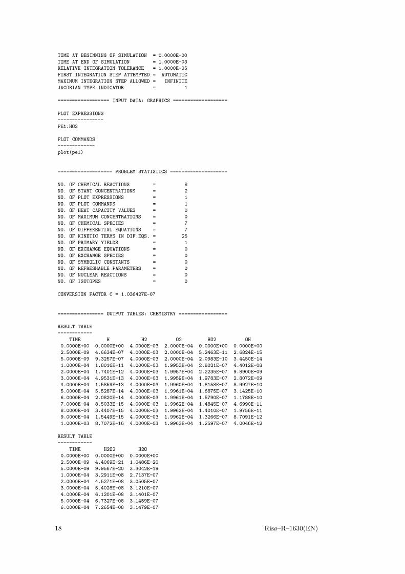
TIME AT BEGINNING OF SIMULATION = 0.0000E+00

TIME AT END OF SIMULATION = 1.0000E-03

RELATIVE INTEGRATION TOLERANCE = 1.0000E-05

FIRST INTEGRATION STEP ATTEMPTED = AUTOMATIC

MAXIMUM INTEGRATION STEP ALLOWED = INFINITE

JACOBIAN TYPE INDICATOR = 1

================== INPUT DATA: GRAPHICS ===================

PLOT EXPRESSIONS

----------------

PE1:HO2

PLOT COMMANDS

-------------

plot(pe1)

=================== PROBLEM STATISTICS ====================

NO. OF CHEMICAL REACTIONS = 8

NO. OF START CONCENTRATIONS = 2

NO. OF PLOT EXPRESSIONS = 1

NO. OF PLOT COMMANDS = 1

NO. OF HEAT CAPACITY VALUES = 0

NO. OF MAXIMUM CONCENTRATIONS = 0

NO. OF CHEMICAL SPECIES = 7

NO. OF DIFFERENTIAL EQUATIONS = 7

NO. OF KINETIC TERMS IN DIF.EQS. = 25

NO. OF PRIMARY YIELDS = 1

NO. OF EXCHANGE EQUATIONS = 0

NO. OF EXCHANGE SPECIES = 0

NO. OF SYMBOLIC CONSTANTS = 0

NO. OF REFRESHABLE PARAMETERS = 0

NO. OF NUCLEAR REACTIONS = 0

NO. OF ISOTOPES = 0

CONVERSION FACTOR C = 1.036427E-07

================ OUTPUT TABLES: CHEMISTRY =================

RESULT TABLE

------------

TIME H H2 O2 HO2 OH

0.0000E+00 0.0000E+00 4.0000E-03 2.0000E-04 0.0000E+00 0.0000E+00

2.5000E-09 4.6634E-07 4.0000E-03 2.0000E-04 5.2463E-11 2.6824E-15

5.0000E-09 9.3257E-07 4.0000E-03 2.0000E-04 2.0983E-10 3.4450E-14

1.0000E-04 1.8016E-11 4.0000E-03 1.9953E-04 2.8021E-07 4.4012E-08

2.0000E-04 1.7401E-12 4.0000E-03 1.9957E-04 2.2235E-07 9.8900E-09

3.0000E-04 4.9531E-13 4.0000E-03 1.9959E-04 1.9783E-07 2.8072E-09

4.0000E-04 1.5859E-13 4.0000E-03 1.9960E-04 1.8158E-07 8.9927E-10

5.0000E-04 5.5287E-14 4.0000E-03 1.9961E-04 1.6875E-07 3.1425E-10

6.0000E-04 2.0820E-14 4.0000E-03 1.9961E-04 1.5790E-07 1.1788E-10

7.0000E-04 8.5033E-15 4.0000E-03 1.9962E-04 1.4845E-07 4.6990E-11

8.0000E-04 3.4407E-15 4.0000E-03 1.9962E-04 1.4010E-07 1.9756E-11

9.0000E-04 1.5449E-15 4.0000E-03 1.9962E-04 1.3266E-07 8.7091E-12

1.0000E-03 8.7072E-16 4.0000E-03 1.9963E-04 1.2597E-07 4.0046E-12

RESULT TABLE

------------

TIME H2O2 H2O

0.0000E+00 0.0000E+00 0.0000E+00

2.5000E-09 4.4069E-21 1.0486E-20

5.0000E-09 9.9567E-20 3.3042E-19

1.0000E-04 3.2911E-08 2.7137E-07

2.0000E-04 4.5271E-08 3.0505E-07

3.0000E-04 5.4028E-08 3.1210E-07

4.0000E-04 6.1201E-08 3.1401E-07

5.0000E-04 6.7327E-08 3.1459E-07

6.0000E-04 7.2654E-08 3.1479E-07

18 Risø–R–1630(EN)

7.0000E-04 7.7342E-08 3.1486E-07

8.0000E-04 8.1502E-08 3.1489E-07

9.0000E-04 8.5219E-08 3.1490E-07

1.0000E-03 8.8561E-08 3.1490E-07

=============== END OF CHEMSIMUL COMPUTATION ==============

CPU TIME FOR CHEMSIMUL: 0.05 SEC.

4.2 Graphical output and plot expressions

The modern Windows-based GUI version of CHEMSIMUL has native built-in graphicalprocedures, while the classical program has an interface to the freeware graphics programgnuplot [9] which is in widespread use on many different computers.

CHEMSIMUL may produce a “Graphics Table File” with one column for time, and onecolumn for each of the plot expressions that are specified in the input file.

Plot expressions (PE. . .) are further discussed in Section 7.13. A plot expression may bejust a single species concentration, as PE1:HO2 in our sample case. However, the concept ismuch more versatile, as it supports all the 5 operators +, −, ×, /, and ^ (exponentiation),together with the common mathematical functions and derivation. Plot expressions area useful facility in situations when a researcher wants to plot a curve which is directlycomparable with certain experimental results. An example is the measurement of extinction

E = (εA[A] + εB[B])� (27)

where εA and εB are the extinction coefficients for species A and B, respectively, � is theoptical path length, and [·] denotes concentration.

The plot expressions themselves will only produce the Graphics Table File. To produce anactual plot, a PLOT command should be used (Section 7.13).

4.3 Formal printout of differential equations

The program can give a formal print-out of the differential equation system to be solved.This may be a useful tutorial facility for understanding reaction kinetics. An example ofthis was shown at the end of Section 3.2. The reaction rates are labelled Kn corresponding toreaction REn. Radiolytic zero-order reactions are recognized. The ODE print-out is activatedby the command DIFFEQ, cf. Section 7.7.

5 Additional features

In the following a number of additional CHEMSIMUL features will be described.

5.1 The stoichiometric mass balance

The accurate solution of the differential equation system describing the chemical reactionsrequires an overall conservation of the chemical mass balance. The numerical integrationscheme itself preserves the mass balance, cf. Section 13.2, so there is no need to check formass balance continually. We use instead a static consistency check. If the check fails, thesimulation is halted before integration; this practice has proved useful for detecting input

Risø–R–1630(EN) 19

errors in the write-up of the reaction equations. CHEMSIMUL recognizes each species asan entity with a name. This means that a formal stoichiometric balance does not implyan atom-to-atom balance. But it is possible to perform a partial consistency check basedon the stoichiometric matrix A. This matrix is defined formally in Section 13.1, but itsmeaning is clear from the following example, where the reactions of the H2–O2 combustioncase (24) are written in matrix form as a balance equation:

−2 1 0 0 0 0 0−1 0 −1 1 0 0 0−1 0 0 −1 2 0 00 0 1 −2 0 1 00 0 0 0 −2 1 0

−1 0 0 0 −1 0 10 0 1 −1 −1 0 11 −1 0 0 −1 0 1

HH2O2

HO2OH

H2O2H2O

=

0000000

(28)

It must be possible to satisfy this equation by a set of strictly positive values for the massesof all the elements of the species vector.

The mathematical implementation of the balance check is discussed in Section 13.2.

5.2 Check of electro neutrality

As will be explained in Section 6.3, CHEMSIMUL admits species names with charge desig-nators as e.g. FE[+++] or OH[-]. Such a convention enables the program to check the electroneutrality in the individual reactions. If the electro neutrality is violated the simulation willbe rejected. Like the mass balance check, this feature may be useful in catching errors inthe input data file.

5.3 Maximum concentration values for species

From the computed simulation curves CHEMSIMUL may estimate maximum values forindividual species, cf. the command MAXCON in Section 7.15. This is done by interpolationin the result tables (Section 13.6).

6 Using the program

This chapter and the following contain instructions about using the CHEMSIMUL program.Supplementary information on exchange equations, radiolysis from decaying isotopes, andrefreshable parameters will be given in the subsequent chapters.

6.1 Running the program

You may find information about procurement, installation, and licensing of the interactiveGUI version of CHEMSIMUL on the CHEMSIMUL home page:

www.chemsimul.dk

We expect that users of the “classical” command-driven code, who are already familiarwith the present booklet, will not find it difficult to use the GUI version. On the otherhand we urge new users to get acquainted with Chapters 6 and 7 even if you only plan

20 Risø–R–1630(EN)

to use the GUI, since the two versions work with essentially the same input and outputfiles. In this way we may consider the GUI version as an “advanced editor” for preparingdata and carrying out simulations. For practical reasons we shall for the main part relatethe following descriptions to the classical code, and refer GUI users to the supplementarywebsite information on the CHEMSIMUL home page.

The main computer platform for running CHEMSIMUL is the Windows PC, although theclassical version also runs under Linux. The program has been tested with several brandsof the Windows operating system.

The name of the code file is Chemsimul.exe for the GUI and chem.exe for the classicalversion. No particular installation procedure is needed, apart from storing the executablefile in a suitable folder in your computer. However, a CHEMSIMUL license file with avalid license key is required for the GUI version. The classical command-driven version isfree and runs without license keys or files; it may also be freely redistributed. Consult theCHEMSIMUL home page.

On a Windows PC CHEMSIMUL is typically launched from a desktop icon. With the GUIcode you may then use the screen menus for example to select and edit an input file, andafterwards carry out a simulation and view the graphical output.

The classical version begins by issuing the following request:

ENTER NAME OF INPUT FILE:

You then type the input file name, including its extension (normally .dat), e.g. mycase.dat(when the extension is .dat it may be omitted); the output file will then be namedmycase.res. (With the classical code it is also possible to enter the input file as com-mand line input, i.e. you may type chem mycase.)

The program checks all the input data, and if errors are found it gives an error messagewhich should be sufficient for identifying the error.

CHEMSIMUL has a progress bar which estimates the current fraction of the simulationbeing already completed. This feature is useful for estimating the progress of the integrationprocedure for long simulations.

All CHEMSIMUL computations are performed internally in a precision amounting to about16 decimal digits.

6.2 Graphics interface

When the CHEMSIMUL job is finished, the main results are written to the .res filedescribed in Section 4.1. If there are plot expressions in the input file (cf. Sections 4.2 and7.13), then the program will produce a Graphics Table File whose name will be the nameof the input file with the extension replaced by .tbl.

The GUI version of CHEMSIMUL has its own native graphics procedures built into theprogram. These procedures are easily accessed from the screen menus.

On the other hand, the classical version has a link to the graphics program gnuplot [9], whichis freeware and may be downloaded from the Internet. You should observe that apart fromthe Graphics Table File, CHEMSIMUL will also produce a command file chemgnu.pltwhich is ready for launching in gnuplot.

Alternatively, you may prefer to view the Graphics Table File by means of your own favoritegraphics program.

Risø–R–1630(EN) 21

6.3 Name rules for species and other entities

Chemical species are identified by their names in CHEMSIMUL. Referring to the samplecase of Section 3.2, H, H2, O2, and HO2 are examples of chemical species names. Anotherkind of species are the exchange species defined in Chapter 8. Other named entities arethe symbolic constants mentioned in Section 7.9 and the refreshable parameters (RPs) inSection 7.11.

We shall now give the rules for forming the names of species, symbolic constants (without#), and RPs (without <). Apart from certain restrictions, these names can be chosen freely.The main rule is that they should be alphanumeric and begin with a letter; they maycontain small and capital letters and are interpreted in a case-sensitive way. Internal blanksin names will be squeezed out during the processing. The maximum permitted length of aname is 24 characters. A name cannot be empty.

A few particular CHEMSIMUL names are reserved. They are listed in Table 2 and mustnot be used in other contexts.

Name MeaningTIME Simulation time in sTEMP Temperature (K) of the systemTEMP2 Dual temperature (Section 7.14.3)

Table 2: Reserved names in CHEMSIMUL

Only the upper-case version of these names are reserved.

The totality of chemical and exchange species names, symbolic constants, and RPs, mustall be distinct.

It is allowed to qualify the name by a pair of square brackets containing strings of eitherof the signs + or -, like FE[+++] or OH[-]. This feature enables CHEMSIMUL to checkthe electro neutrality (Section 5.2) and also to estimate the rate constant dependency onthe ionic strength (Section 10.3). It is also permitted to use square brackets as numericalmarkers in names, like A[0] or B[219]; any string of the digits 0 – 9 is accepted. The twomodes may be combined, but not within a single bracket pair. Thus A[2][+] would belegal but not A[2+]. Square brackets must be properly paired. At most one pair of bracketswith either + or - can occur in a name, and at most one pair with digits. Empty bracketsare illegal, and so is nested use of square brackets.

Normal parenthesis pairs (...) are also allowed, and they can even be nested in morethan one level. The pairing must hold on all levels. Square brackets cannot occur withinparentheses on any level, and vice versa. Some examples of names containing parenthesesare given below:

- Ca(OH)2[0]: Neutral aqueous complex, to be distinguished from the solid phase Ca(OH)2.

- Fe(OH)4[-]: Mono-charged negative ion, allows a condensed and more traditional writ-ing of the complex FeOHOHOHOH[-].

- Fe(OH)2[+]: Mono-charged positive ion, immediately recognizable from the bi-chargedpositive ion FeOH[++]; here the writing of FeOH2+ would be ambiguous.

- Al4(Fe(CN)6)3(H2O)17: This name has several pairs of parentheses, one of these beingnested.

22 Risø–R–1630(EN)

6.4 Regular expressions in CHEMSIMUL

CHEMSIMUL supports several kinds of expressions. Section 7.11 gives the definition ofrefreshable parameters (RPs), e.g.

<z1 = a + b*z2

In Section 7.13 the plot expressions are mentioned, with the following simple example:

PE2: TEMP-273.15

Finally, in Chapter 8, exchange expressions are discussed. An example is:

d(N2g)/dt = coef * ((H2g0+N2g0)^2-(H2g+N2g)^2)/(H2g+N2g)

Common for the RP definition after =, the plot expression after :, and the exchange equationafter =, is that each of them is a so-called regular expression. The rules for constructingregular expressions are as follows:

Regular expressions are general arithmetic expressions, which may be composed of thenamed entities of Section 6.3. Blank spaces in expressions are insignificant. When a speciesname occurs, say HO2, it is understood that the actual concentration of the species issubstituted. Chemical and exchange species may enter, and so may symbolic constants(without #) and RPs (without <). Moreover, the reserved names in Table 2 can be used inthe same way as species.

Allowed operators are sum (+), difference (-), product (*), division (/), and exponentiation(^). Operations proceed from left to right except for repeated exponentiations which areevaluated from right to left. Parentheses may overrule the calculation order in the usualway. The multiplication operator cannot be omitted. Thus writing (a+b)(c+d) or 2a isillegal; you must write (a+b)*(c+d) and 2*a.

A number of standard mathematical functions are available, cf. Table 3:

Function name Meaningcos cosine with argument in radianscosh hyperbolic cosineexp exponential functionln natural logaritm (base e)

log10 logarithm with base 10sin sine with argument in radianssinh hyperbolic sinesqrt square roottan tangent with argument in radianstanh hyperbolic tangent

Table 3: Mathematical functions in CHEMSIMUL regular expressions

Note that the exponentiation operator (^) requires positive arguments. If you just needsquare or cube operations, you may write A*A or A*A*A.

Using two consecutive operators as in 10^ -(a+b) is not allowed; you should instead write10^ (-(a+b)).

Case rules: The reserved names in Table 2 must all be in upper case. The mathematicalfunctions may be in either case.

Braced items in regular expressions can be used to include certain other entities that areconstant during the simulation, e.g. you may write the following plot expression:

Risø–R–1630(EN) 23

PE1: FE[+++] * (1 - TIME/{TEND})

This example contains the command value TEND (Section 7.6). The actual input value ofTEND is simply substituted into the expression. The syntax requires that TEND be enclosedin curly braces {}. Two other commands, TSTART and CONVERT (Sections 7.6 and 7.15), canbe used in the same way. Note that if an unassigned command is used in the expression,its default value applies. (This is 0 for TSTART and 1.036427 · 10−7 for CONVERT). Moreover,a primary yield (G-value) can enter a regular expression, as for example in

PE3: {g(H2)} - 0.2*{TEND}

or

PE4: {CONVERT} * {GG(H2)} * {DOSERATEG}

(where an Isotope Block (Chapter 9) was used in the last example).

Braced items are case insensitive, apart from species names.

7 Input file

We shall now describe how a CHEMSIMUL input file is constructed. The description per-tains to the GUI as well as the classical version of the program. Naturally, the inputcapabilities are richer and more versatile in the GUI version, cf. the CHEMSIMUL web-site www.chemsimul.dk. Moreover, the GUI has powerful editing tools for constructing andmodifying the input file. Hence, in daily use you need not be concerned about the correctpreparation of the input file. Nevertheless all CHEMSIMUL users should read the presentchapter in order to get a general understanding of the capabilities and the functionality ofthe program.

The input file is just a standard text file containing a number of lines or records. No linecan exceed 1023 characters in length. Only standard text characters (ASCII) are applied.Hence, if you are using the classical version, you may use any text editor to edit yourCHEMSIMUL input files; in contrast the GUI version will as mentioned above take care ofthe file editing itself.

The input data contain commands that are identified by well-defined character strings.For example, the reaction equations always begin with RE, the start concentration of re-actants always with CON, etc. CHEMSIMUL is case insensitive for command typing, butcase sensitive for typing names of species and other entities. Blank spaces in commands areignored.

You can insert comment lines freely in the input file; such lines begin with an asterisk(*). For example, you may use such comments to make commands inoperative. Blanklines are also considered as comments. Yet another way of stating comments is to writean exclamation mark (!) after any command, which means that only the text after ! isconsidered as a comment. In particular ! can be used instead of *. Examples of comments:

* This is a comment

*save

RE13:H+O[-]=OH[-];A=2E10 ! Bjergbakke and Draganic 1989

24 Risø–R–1630(EN)

A CHEMSIMUL input file terminates with the command $ENDDATA; any records after$ENDDATA are ignored.

The input data file for CHEMISIMUL is organized in data blocks. A data block correpondsto a screen tab in the GUI program. In subsequent sections we shall describe the contentsof each block. To illustrate we begin by reproducing the complete input data file for thecombustion sample test with pulse irradiation that produced the output in Section 4.1:

7.1 Sample data set

$IdentificationSimulation of an H2 - O2 explosion with the following parameters:5 mbar O2 + 100 mbar H2 + Ar to 1 atm. k8=4000.$Chemical reactionsRE1: H+H=H2; A=4.0E7RE2: H+O2=HO2; A=4.5E8RE3: H+HO2=OH+OH; A=6.5E10RE4: HO2+HO2=H2O2+O2; A=2.0E9RE5: OH+OH=H2O2; A=4.0E9RE6: H+OH=H2O; A=1.0E10RE7: OH+HO2=H2O+O2; A=6.0E10RE8: OH+H2=H2O+H; A=4.0E3$IrradiationTOTALDOSE=9.0 ! GyRADTIME=5.0E-9G(H)=1.0$ConcentrationsCON(O2)=2.0E-4CON(H2)=4.0E-3$Output controlPRINTS=12*DIFFEQRADPRS=2$IntegrationTEND=1.0E-3$GraphicsPE1:HO2plot(pe1)$ENDDATA

7.2 General rules for data blocks

The sample case shown above has 7 data blocks. (The trailing $ENDDATA record is notconsidered as a data block.) Each block begins with a block header whose first character is$. In this case the block headers are $Identification, $Chemical reactions, and so on.Below we give general rules for making the data blocks:

There are altogether 13 data blocks available. They are initiated by block headers as follows:

$ Identification$ Chemical reactions$ Concentrations$ Integration

Risø–R–1630(EN) 25

$ Output control$ Irradiation$ Symbolic constants$ Exchange equations$ Refreshable parameters$ Isotope$ Graphics$ Tabular data$ Miscellaneous

As other CHEMSIMUL commands, these block headers are interpreted in a case-insensitiveway, and blanks will be suppressed. Only the first 8 nonblank characters (including $) aresignificant. This means that you may write e.g. $CHEMICAL KINETICS, $chemical system,$exchange, $refreshable quantities etc., if you like.

Blocks may come in any order, and so may items within blocks (apart from a few exceptionsto be mentioned later).

Except within tables, comment and blank lines are allowed anywhere in the data file,including prior to the first data block.

All blocks are optional; they may be omitted, or they may be empty.

7.3 The Identification Block

The entire content of the $ IDENTIFICATION block will be reproduced verbatim in thebeginning of the output file. In particular comment lines are retained in the print. The firsttext line in the block is used for headlines in plots. Example:

$ IdentificationCarbonation of pure water by air, 1 week.Cylindrical beaker with gaseous sky.EXPERIMENTAL CONDITIONS:Gas volume = 0.001 m3.Liquid volume = 0.001 m3.Interfacial area liq/gas = 0.01 m2.Height of water = 0.1 m.

7.4 The Chemical Reactions Block

The $ CHEMICAL REACTIONS block is the block which contains the system of chemicalreaction equations.

Each reaction equation is prefixed with a unique identification REn:, where RE meansReaction Equation and n is the equation identification number. The reaction equation ter-minates with a semicolon (;) and is followed by the thermodynamics constants A, EA, B(Section 2.6), and the heat of reaction qr = Q (Section 2.7), separated by a comma (,).Here EA, B, Q are optional, but A is required; if EA and B are omitted, then A just means thereaction constant k. Interspersed blanks for enhancing readability are allowed. Example:

$ CHEMICAL REACTIONSRE3: H[+]+OH[-]=H2O; A=2.35E13, EA=3RE2: H+HO2=OH+OH; A=2.5E11, EA=1.9, Q=38.3RE64: 2*OH=H2O2; A=6.0E9

26 Risø–R–1630(EN)

Note that it is not necessary to number the reactions consecutively. Combined with the useof comment lines (∗), this flexibility may be exploited to mask out single reactions, or toestablish data bases on certain reaction mechanisms.

The stoichiometric constants are integers, while the rate constants are real numbers; theirvalues can be entered in “free format”. CHEMSIMUL supports “scientific notation” forexponents, using the symbol E (or e) for the exponent, i.e. 1.4E11 means 1.4 · 1011. Notethat E11 is an illegal specification, but 1E11 is okay. The maximum order of a chemicalreaction to be simulated is 2, i.e. up to 2 reactants can be written on the left hand side ofthe reaction equations, but there are virtually no restrictions on the number of productson the right hand side. There are no bounds on the number of reactions or species.

The terms A, EA and B are related to the modified Arrhenius expression for the reactionrate given in Section 2.6, k = AT β exp(−Ea/(RT )), where T is the temperature in K: A= A, EA = Ea, and B = β. The factor T β is included for gas phase kinetics, with β beingan empirical exponent. A is the so-called frequency factor, and Ea the activation energy.When activation energies are used, you must ensure that the gas constant R is given in aunit which is compatible with Ea, cf. Section 7.15.

By using the phrase A=TABLE it is possible to use tables of rate constants versus temperature.This is explained in Section 7.14.2. It is also possible to set a reaction rate equal to arefreshable parameter (RP) by writing say A = <z1, see Section 7.11.

The term Q corresponds to the heat of reaction qr for reaction r, as described in Section 2.7.Note that the heat of reaction and the heat capacity values (HCV in Section 7.15) must bein compatible units; see also Table 1 in Section 2.1.

Default values for EA, B, and Q are zero, while the input of A as previously mentioned ismandatory for all reactions. The four specifiers may come in any order.

7.5 The Concentrations Block

The $ CONCENTRATIONS block contains initial values of the concentration of species in thesimulation system.

Each command has the form CON(X) = . . . and gives the value of the start concentrationfor the species X. Example:

$Concentrationscon(O2) = 2.0e-4con(H2) = 4.0e-3

Default values of all initial concentrations are zero. The concentration unit is mol × dm−3

or molecules × cm−3, cf. Table 1 in Section 2.1.

Both the initial concentrations of chemical species and exchange species (Section 7.10 andChapter 8) should be given in this block.

7.6 The Integration Block

The $ INTEGRATION block contains commands related to the simulation and the numericalsolution of the corresponding differential equations. Example:

$Integrationeps = 1.0e-6

Risø–R–1630(EN) 27

fststp = 1.0e-8hmax = 0.001jt = 1tend = 12

These commands have the following meaning (alphabetic order):

EPS

The command EPS = εrel gives the relative accuracy εrel in the integration routine (DL-SODA). Its default value is 1.0 · 10−5.

Hint: In most cases the computing time increases when EPS is made smaller. Difficult casesmay require adjustment of one or more of the input data EPS, FSTSTP, HMAX.

FSTSTP

The command FSTSTP = h0 gives the initial integration step h0, measured in s. The solverhas automatic step size control and is able to estimate its own initial step by default.

Hint: To see the actual first step, use the MATHINFO command (Section 7.7). The experienceduser may sometimes save time by setting a larger FSTSTP. On the other hand, difficult casesmay require very small values of FSTSTP to prevent integration failures. In such cases it mayalso be necessary to adjust EPS and/or HMAX.

HMAX

The command HMAX = hmax gives the maximum allowed length hmax of an integration stepin s. By default hmax = ∞ which means that the solver is free to use as large steps as itwants.

Hint: To see the maximal step actually taken by the code, use the MATHINFO command (Sec-tion 7.7). The experienced user may sometimes want to set HMAX to enhance the precision.This may occasionally be needed to prevent integration failures. In such cases it may alsobe necessary to adjust EPS and/or FSTSTP.

JT

Indicator for Jacobian type. As explained in Section 13.4, the integrator may need theJacobian df/dy of the differential equation system. JT = 1 is the standard choice and thedefault setting in CHEMSIMUL. Other possible choices are JT = 2 and JT = 3. All threeoptions are explained and discussed in Section 13.4.

TEND

The command TEND = tend gives the end time tend in s for the simulation. By defaulttend = 0.

Note: TEND is an absolute time. It is not necessarily equal to the time duration of thesimulation which is TEND − TSTART, cf. below.

28 Risø–R–1630(EN)

TSTART

The command TSTART = tstart gives the initial time tstart in s for the simulation. TSTARTmust not be negative. By default tstart = 0.

Hint: TSTART may be useful in applications involving restart.

7.7 The Output Control Block

The $ OUTPUT CONTROL block contains commands which control the printed output. Ex-ample:

$Output controlderivative(OH,H2)diffeqdig = 3linele = 132mathinfoprintonly(H2O2,H,TEMP)printonly_rp(rp1,rp2)prints = 25radprs = 5save

These commands have the following meaning (alphabetic order):

DERIVATIVE

The command DERIVATIVE(...) enables the printing of selected derivatives in a specialtable after the normal result table. The selected species should be entered as a comma-separated list in parantheses. TEMP, when relevant, may be included in the list (uppercase), and so may exchange species (Chapter 8). If no DERIVATIVE command is present, noderivative table is produced. Only one DERIVATIVE command is allowed.

Hint: Computing a numerical estimate of the derivative is more difficult than computing thequantity itself. To obtain a sufficient accuracy it may be necessary to choose a smaller valueof EPS than its default value 1.0 · 10−5. Precision enhancement can also be accomplished bythe HMAX command. See also Section 13.5.

DIFFEQ

If this command is written in the input file, then the differential equation system will beprinted. By default the system is not printed. See also Sections 4.3 and 3.2. Zero-orderterms with G-values are included in the print-out (without the conversion factor c), butexchange equations (Chapter 8) are omitted.

DIG

This command defines the number of significant digits in the result table of CHEMSIMUL.By default DIG = 5. It is the format of the main output tables that is adjustable in thisway. Other CHEMSIMUL results are presented in fixed formats.

Risø–R–1630(EN) 29

LINELE

The command LINELE = � defines the number of characters per line in the main result table(and the output generated by DIFFEQ). By default � = 72. This is also the least possiblevalue.

MATHINFO

This command causes some statistics about the integration to be printed in the result file.Furthermore, an additional file message.ode is created by the solver with more detailsabout the integration. By default this feature is disabled.

PRINTONLY

The command PRINTONLY(...) restricts the printing of species concentrations in the re-sult table to certain selected species. The selected species should be entered as a comma-separated list in parantheses. TEMP, when relevant, may be included in the list (upper case).If no PRINTONLY command is present, then all species will be printed. Only one PRINTONLYcommand is allowed.

PRINTONLY RP

The command PRINTONLY RP(...) is analogous to PRINTONLY(...) but pertains to theprinting of refreshable parameters (RPs) (Section 7.11).

PRINTS

The command PRINTS = n defines the total number of output lines in the result table afterthe initial time, such that n + 1 lines are actually printed, with PRINTS = n print intervals.Each line contains the time and the simulation results belonging to that time. In case ofirradiation pulse(s) PRINTS includes RADPRS (see below), i.e. 0 ≤ RADPRS ≤ PRINTS. Bydefault PRINTS = 0.

RADPRS

This command controls the number of lines printed during irradiation. For a single pulseRADPRS= nr defines the number nr of equal time intervals in the result table during theirradiation pulse. For a pulse train (NRR > 1) the total irradiation period TTRAIN is dividedin RADPRS= nr equal subintervals for printing (Section 2.3). Note: RADPRS must satisfy thecondition 0 ≤ RADPRS ≤ PRINTS. Default value is 0. See also PRINTS.

SAVE

This command causes the computed results to be written to a save file by the end of thesimulation. You may use the save file as a tool for preparing a “restart by hand” by usingcopy and paste technique. (We have excluded the possibility of making automatic restartsin CHEMSIMUL, because it might be difficult for the user to keep track of the exactconditions for the restart simulation.) By default the save file will bear the same name as

30 Risø–R–1630(EN)

the main input file, only with the extension replaced by .sav, but you can overrule this bygiving another file name as a parameter to SAVE, for example:

save pp2.dmp

For thermodynamic simulations also the temperature TEMP will be saved. Some hints forexploiting the save facility to do manual restarts are given in Section 11.6.

The save file will have the following format:

*** CHEMSIMUL SAVE FILE FOR MANUAL RESTART*** pp2.dat 30-MAY-2008 16:14*** CASE:PAGSBERG TEST OF B AND Q;****** KEY NUMBERS FOR SIMULATION:*** TIME AT BEGINNING OF SIMULATION..= 0.000000E+00*** TIME AT END OF SIMULATION........= 2.000000E-04*** RELATIVE INTEGRATION TOLERANCE...= 1.000000E-05*** CONVERSION FACTOR C..............= 1.036427E-06****** FINAL CONCENTRATIONS = NEXT INITIAL CONCENTRATION BY COPY/PASTE:CON(OH) = 8.5774520818151815E-08CON(P) = 4.7532617219312779E-07CON(AE) = 0.0000000000000000E+00CON(AR) = 4.0001036426865207E-02TEMP = 5.1882847677544373E+02****** ENDSAVE ... END OF SAVE FILE

Record 1 is a fixed header, record 2 contains the name of the mother input file and atime stamp, and record 3 is the same as the first record in the Identification Block (Sec-tion 7.3). Then some key numbers for the simulation follow. Note that the two time valuescorrespond to TSTART and TEND, respectively, and are absolute times; their difference TEND− TSTART equals the duration of the simulation. Next all the final concentration recordsfollow, possibly a TEMP record, and finally an ENDSAVE record.

Note that when you copy CON records from a save file to a new input file in order to domanual restart, you can either let these replace the old CON records, or you may insert thenew records after the old ones (but still in the Concentrations Block). In the latter casethe new CON values overrule the old values.

Also note that the phrase “concentrations” should here be understood in a general sence,since these may also refer to exchange species (Section 7.10 and Chapter 8).

If you are using an Isotope Block, a revised Isotope Block will be saved just before theENDSAVE record, see Section 9.5.5.

7.8 The Irradiation Block

The $ IRRADIATION block contains various commands related to external pulse or pulse-train irradiation, cf. Section 2.3. Example:

$IrradiationG(H) = 1.0G(OH) = 2.0

Risø–R–1630(EN) 31

nrr = 5radtime = 1e-6ttrain = 2.0e-5totaldose = 3.7

These commands have the following meaning (alphabetic order):

G

This command is used for entering primary yields or ‘G-values’ for external pulse irradiationfor one or more species. See the example above for the syntax.

The primary yields are used if the reaction system is irradiated e.g. by high-energetic elec-trons or by gamma rays. They were introduced in Section 2.2, and are in units of moleculesper heV. See in particular formula (1). The primary yields default to 0 in CHEMSIMUL.

The G-value input has been generalized to refreshable parameters (RPs) (Section 7.11).Thus you may write

G(OH) = <goh

where goh is supposed to be an RP defined in the Refreshable Parameters Block, for exampleby the equation

<goh = 2.0 + 0.0015*TEMP

This will cause G(OH) itself to be refreshed during simulation. (You can not, however, usethe direct form G(OH) = 2.0 + 0.0015*TEMP.)

When using this facility you should ensure that the mass balance is respected for theG-values, see Section 11.4.

Note that if you associate a primary yield with an RP, as in G(H2) = <ghydrogen, youcannot use the braced-item form {G(H2)} in a regular expression, as we did in the plotexpression PE3 in Section 6.4; this presupposed that G(H2) was assigned a numerical value.Instead you should write

PE3: <ghydrogen - 0.2*{TEND}

Chemical species as well as exchange species (Section 7.10 and Chapter 8) may be associatedwith G-values.

NRR

This is the number of individual pulses in a pulse train (Section 2.3). Default value is 1 incase of irradiation and otherwise 0. Thus the command is only needed when there are morethan one pulse.

RADTIME

RADTIME= tr gives the irradiation time tr in s for the rectangular pulse (or for each pulse ifthere are more than 1, Section 2.3). Default value is zero.

32 Risø–R–1630(EN)

TOTALDOSE

The command TOTALDOSE = D gives the total irradiation dose D in Gy during the irradia-tion time for the rectangular pulse (or the total train for more than one pulse, Section 2.3).

If you prefer to work with krad as the dose unit, you should use the command DOSEUNIT inSection 7.15.

TTRAIN

This command is used in case of pulse-train irradiation, see Figure 1 in Section 2.3. TTRAIN= ttrain is given in s and is equal to the time duration of the total pulse train, includingthe pulse pauses. See also the command NRR. TTRAIN is required when NRR > 1. When NRR= 1 TTRAIN is automatically set to RADTIME and need not be set by the user.

7.9 The Symbolic Constants Block

In order to improve integrity and readability of the input data and avoid repetition of nu-merical constants, CHEMSIMUL admits the use of symbolic constants which are names thatare assigned fixed numerical values. The symbolic constants may enter all regular expres-sions, i.e. exchange equations (Chapter 8), plot expressions (Section 7.13), and definitionsof refreshable parameters (Section 7.11).

Symbolic constants are declared in a $ SYMBOLIC CONSTANTS block. The name of eachconstant must comply with the name rules given in section 6.3 and must be preceded bythe token # in its declaration. On the other hand, when the constant is used in expressionsas mentioned above, the name is given without the #. Example:

$Symbolic constants#coef1 = 1.05E-8#coef2 = 2.13E-6

As explained in Section 10.3 CHEMSIMUL associates a particular meaning with certainsymbolic constants, provided the IONIC command in Section 7.15 is set. These constantsall begin with MM followed by species names; they represent molar masses, cf. Section 2.9.(Without IONIC, constants with these names can still be used, but without the specialmeaning.)

7.10 The Exchange Equations Block

The $ EXCHANGE EQUATIONS block contains input for the so-called exchange equations.These equations can be used for describing transport processes and other heterogeneousphenomena. They may also be used in the study of general dynamic systems. An exampleof such a block is given below:

$exchange equations* Hydrogen convectiond(H2g)/dt = 2.11E-8*H2g * ((H2g0+N2g0)^2-(H2g+N2g)^2)/(H2g+N2g)d(H2ge)/dt = -2.11E-8*H2g * ((H2g0+N2g0)^2-(H2g+N2g)^2)/(H2g+N2g)* Nitrogen convectiond(N2g)/dt = 1.05E-8*N2g * ((H2g0+N2g0)^2-(H2g+N2g)^2)/(H2g+N2g)d(N2ge)/dt = -1.05E-8*N2g * ((H2g0+N2g0)^2-(H2g+N2g)^2)/(H2g+N2g)

Risø–R–1630(EN) 33

* Add neutral instructions for exchange species H2g0 and N2g0d(H2g0)/dt = 0d(N2g0)/dt = 0

On the left-hand side of each exchange equation the time derivative of some species con-centration is stated in the syntax shown. This time derivative should be understood asthe contribution to the production rate from some specific process. The expressions onthe right-hand side are constructed as regular expressions. You should consult Section 6.4where the syntax of regular expressions are given, and where all the possible constituentelements are mentioned. We call the species that occur only in the exchange equationsexchange species, while the others are chemical species. Both kinds are allowed to occur oneither side of an exchange equation. We stress again that an exchange equation is not itselfa differential equation. It accounts for a particular contribution to a production rate for aspecies; other contributions may come from the chemical kinetics or other exchange equa-tions. Exchange equations are allowed to be additive, which means that the same speciesX may occur on the left-hand side of more than one exchange equation. In such a caseCHEMSIMUL adds the corresponding right-hand sides together and uses the sum as thetotal exchange contribution to X. This feature may also be useful in breaking up very longexpressions into several right-hand side addents. For reasons of data check and integrity,CHEMSIMUL requires that each of the exchange species be mentioned on the left side ofan exchange equation; if necessary “neutral instructions” must be given as shown in ourexample for H2g0 and N2g0.

The concept of “concentrations” is formally retained for the exchange species too, eventhough their true units might be something else. With this interpretation, initial concen-trations of exchange species can be defined exactly as for the chemical species by using CON,e.g.

CON(H2g0)=2.09E-8

Like for chemical species the initial concentrations of exchange species are 0 by default.Names of exchange species are formed in the same way as for chemical species (Section 6.3).Often the use of symbolic constants are useful in exchange equations. As an example wemay take the first two equations shown above. Assuming we have defined the symbolicconstant

#coefh = 2.11E-8

in the Symbolic Constants Block, we may write

d(H2g)/dt = coefh * H2g * ((H2g0+N2g0)^2-(H2g+N2g)^2)/(H2g+N2g)d(H2ge)/dt = -coefh * H2g * ((H2g0+N2g0)^2-(H2g+N2g)^2)/(H2g+N2g)

More examples of the use of exchange equations are shown in Chapter 8.

7.11 The Refreshable Parameters Block

CHEMSIMUL supports the so-called refreshable parameters (RPs) which are defined byalgebraic equations. Such equations are not themselves differential equations but are in-terlinked to the ODE (ordinary differential equation) system during the simulation. Theirvalues are refreshed as the integration proceeds.

Refreshable parameters are useful in case of long-duration simulations when the modelcontains certain physical entities as for example the density ρliq, the molality, and the

34 Risø–R–1630(EN)

CUC , which are supposed to change continually with time. See Sections 2.9 and 2.10 andChapter 10.

In general it is not an easy task to solve combined sets of differential and algebraic equations(DAE); special methods and software are required for such systems (Asher and Petzold [10]).But if we impose certain restrictions on the RPs it is indeed possible to interface them tothe ODE solver (in our case DLSODA). In CHEMSIMUL the refreshable parameters mustbe a chain of explicit equations. An explicit RP definition of say z1 has the form

z1 = f(z2, z3, . . . ; other parameters) (29)

where z2, z3, . . . are other RPs, and “other parameters” may include e.g. current speciesconcentrations and symbolic constants. Implicit equations in the RPs are not supported byCHEMSIMUL.

The input write-up of the RPs should be made in the $ REFRESHABLE PARAMETERS block.We give a small example of a complete data file to show the syntax:

$identificationArtificial test case with refreshable parameters$chemical reactionsRE1:R1+R2=R3;A=<z1$concentrationsCON(R1)=4.1992D0CON(R2)=1.6941D0CON(R3)=0.8852D0$integrationTEND=10$output controlPRINTS=10$symbolic constants#a = 1.3816#b = 0.2377$refreshable parameters<z1 = a + b*z2<z2 = 1/R1 - a/b$graphicspe1: z1pe2: z2plot(pe1,pe2)$enddata

We see that in the $ REFRESHABLE PARAMETERS block two RPs z1 and z2 are defined bypreceding their names with the token <, and writing their defining expressions on the right-hand side. Each right-hand side may contain (chemical or exchange) species concentrations(here R1), temperature, symbolic constants (here a and b), and other RPs (here z2). Notethat RPs on the right-hand side should not be preceded by <.

The example also illustrates that RPs may provide feedback to the chemical kinetics. Inthis case the formation of the species R3 is enabled by equating the reaction rate to an RPz1 using the following syntax:

RE1: R1 + R2 = R3; A = <z1

This syntax can not be extended to general expressions, i.e. writing A = <z1 + <z2 wouldbe illegal.

Risø–R–1630(EN) 35

RP names should comply with the naming rules in Section 6.3. An RP expression must bea regular expression. You should consult Section 6.4 where the syntax of regular expressionsare given, and where all the possible constituent elements are mentioned. In particular, anRP expression may contain other RPs.

Here is a valid example of a more complicated RP:

<G1 = 10^(-0.5092*(SQRT(IS)/(1+SQRT(IS))-0.3*IS))

(But note that the expression

<LOG10(G1) = -0.5092*(SQRT(IS)/(1+SQRT(IS))-0.3*IS)

would be invalid because it is not explicit, since G1 occurs as the argument of a logarithm.)

The RP values obtained during simulation are printed in a separate output table. See,however, the command PRINTONLY RP in Section 7.7.

As our test example shows, RPs are allowed to enter plot expressions. They may also occurin exchange equations.

RPs may also be utilized as a means of storing current accounts when computing expres-sions. This may give reductions in write-up as well as computing time. As an example,consider the two first exchange equations in the example of Section 7.9. These may bewritten

d(H2g)/dt = rhsH2gd(H2ge)/dt = -rhsH2g

provided the RP definition

<rhsH2g = 2.11E-8*H2g * ((H2g0+N2g0)^2-(H2g+N2g)^2)/(H2g+N2g)

is included in the $ REFRESHABLE PARAMETERS block.

The RPs in the $ REFRESHABLE PARAMETERS block must form a resolvable chain of explicitequations, which means that it should be possible to evaluate all the RPs in turn by explicitformulas without ever encountering an RP that is not already defined. In particular, no RPdefinition must be “circular”, i.e. it must not reference itself directly or indirectly. Findinga resolvable chain may require a reordering (“chaining”) of the RP definitions. However,you need not be concerned with the order in which you mention the RPs in your input file;the program will find a proper permutation if necessary to do the ordering task. Details ofCHEMSIMUL’s mathematical handling of RPs are given in Sections 13.9 and 13.10.

7.12 The Isotope Block

The $ ISOTOPE block contains input for simulating radiolysis from decaying isotopes. Dueto the importance of this feature, it will be described in detail in Chapter 9. Here we shalljust list a real case example of such a block:

$ ISOTOPE

* Nuclear reactions, decay constants (s-1) and initial dose rates (Gy/s)NR1:Pu241=Am241; k=1.53066E-9, DB=2.80E-11NR2:Am241=Np237; k=5.07626E-11, DA=4.12E-5, DG=1.70E-9

36 Risø–R–1630(EN)

NR3:Cs137=Ba137m; k=6.904574E-10, DB=6.29E-5NR4:Cs137=Ba137; k=4.126939E-11, DB=8.98E-6NR5:Ba137m=Ba137; k=4.526823E-3, DG=2.15E-4

* Initial activities (Bq)ACTIVITY(Pu241)=5.2E12ACTIVITY(Am241)=5.0E10ACTIVITY(Cs137)=1.755E13ACTIVITY(Ba137m)=1.755E13

* Primary yields for alpha radiation (molecules/heV)GA(H2)=1.30GA(E[-])=0.06GA(H)=0.21GA(H[+])=0.06GA(OH)=0.24GA(H2O2)=0.985GA(HO2)=0.22GA(H2O)=-2.71

* Primary yields for beta radiation (molecules/heV)GB(H2)=0.45GB(E[-])=2.66GB(H)=0.55GB(OH[-])=0.10GB(H[+])=2.76GB(OH)=2.67GB(H2O2)=0.72GB(H2O)=-6.97

* Primary yields for gamma radiation (molecules/heV)GG(H2)=0.45GG(E[-])=2.66GG(H)=0.55GG(OH[-])=0.10GG(H[+])=2.76GG(OH)=2.67GG(H2O2)=0.72GG(H2O)=-6.97

* Specific isotopic dose ratesDOSERATEB(Pu241)DOSERATEA(Am241)

* Decay print of all activities and amounts (not activated here)* DECAYPRINT

7.13 The Graphics Block

The GUI version of CHEMSIMUL has richer graphical facilities than the classical program,see the website www.chemsimul.dk. However, the structure of the graphical input is thesame in the two versions.

Risø–R–1630(EN) 37

The $ GRAPHICS block may contain plot expressions and plot commands, cf. Section 4.2.Furthermore, there may be one or more data file references (DF...) for plotting external datafiles. Example:

$GraphicsPE1:HO2PE2:OHPE3:HO2 + OHDF1:ho2resul.datplot(pe1,pe2,pe3)plot(pe1,df1)

These commands have the following meaning (alphabetic order):

DF

Each data file reference is initiated by DF followed by a number and a colon. The numbersneed not come in natural order but they must be distinct. Items like DF1 are called datafile headers. After the colon follows the name of a file containing a table, which typicallycontains experimental data.

The GUI version is much more flexible than the classical with respect to the interpretationof external data files. First, you should notice that the classical version requires the fileto reside in the same folder as the executable program file and be referred by its localname; in constrast the GUI version has a full-fledged file reference system with completepath designations. Next, in the classical version only files with simple xy-tables in textformat are allowed, while the GUI also supports multi-column table files in other formatse.g. Excel. You are advised to consult www.chemsimul.dk. Below we describe the restrictedfeatures accepted by the classical version.

The referenced file must contain pairs of data in two columns separated by an optionalcomma and at least one space. In the first column we must always have the time values (s),while the second contains the experimental (or other) data values. Example of such a file:

0.00000 0.000.00025 1.65e-70.00050 1.42e-70.00075 1.30e-70.00100 1.15e-70.00125 1.11e-70.00150 1.03e-70.00175 0.96e-70.00200 0.84e-7

To launch a plot with external data files, you should use the PLOT command.

PE

Plot expressions, which were mentioned in Section 4.2, will not by themselves create anyplots, but only a Graphics Table File. To make the plots, you should use the PLOT command.

Each plot expression is initiated by PE followed by a number and a colon. The numbersneed not come in natural order but they must be distinct. Items like PE1 are called plot-expression headers. The expression after the colon must be a regular expression. You should

38 Risø–R–1630(EN)

consult Section 6.4 where the syntax of regular expressions is given, and where all the pos-sible constituent elements are mentioned. In this way plot expressions admit quite generalarithmetic expressions in the species concentrations and other entities to be plotted asfunctions of time.

Plot expressions allow one extension of the syntax of regular expressions: You can handlederivatives of species (incl. TEMP), simply by appending a trailing ’ mark, as H2O2’. Thusthe following plot expression is legal:

PE3: 210*H2O2’+1800*O2[-]-FE[+++]^1.5/220-TIME+log10(OH)

The remarks given as “Hint” for the DERIVATIVE command, apply here, too (Section 7.7).

PLOT

Plot commands are needed to produce actual plots based on the Graphics Table File. Eachplot command creates one graphical page or frame. A single frame may contain severalcurves. The general structure of the plot command is:

plot (independent variable ; dependent variables : options)

Thus we have three argument groups, 1, 2, and 3. The semicolon may be omitted whichmeans that the indepedent variable defaults to TIME. Alternatively, you may explicitelystate TIME (upper case), or one of the plot-expression headers, say pe1, as independentvariable. The colon may also be omitted, meaning default options. Argument groups 2 and3 may contain comma-separated lists of items. The items in group 2 are plot expressionheaders and data file headers in any order.

The possible options in the classical program are XLOG, YLOG, MARK, GRID. XLOG producesa logarithmic scale on the x-axis, and YLOG does the same on the y-axis; by default bothaxes are linear. MARK produces curve marks which might be useful for discerning curvesin black-and-white representation, and GRID establishes a set of grid lines on the frame.Options are interpreted in a case-insensitive way. More options are available in the GUIversion, see www.chemsimul.dk.

The capabilities of the PLOT command are illustrated by the following examples:

plot(pe1,pe2) ! plots pe1 and pe2 as functions of TIME; default options.plot(TIME;pe1,pe2) ! same as above; note that TIME must be uppercase.plot(pe1;pe2) ! classical xy-plot with pe1 as independent variable.plot(pe5,pe2,pe3:grid,mark) ! plot with grid lines and curve marks.plot(pe1,pe2,pe3:xlog) ! logarithmic TIME scale.plot(pe1,pe4:ylog) ! logarithmic y scale i.e. for pe1 and pe4.plot(pe1:xlog,ylog) ! logarithmic scales for both TIME and pe1.plot(pe1,df1) ! co-plotting a plot expression with an experimental file.

When TIME is not the independent variable, the options XLOG and YLOG have no effect inthe classical program version.

7.14 The Tabular Data Block

CHEMSIMUL accepts certain data in tabular form. We shall first give the general rules forwriting input tables in CHEMSIMUL and then describe some particular kinds of tables.

Risø–R–1630(EN) 39

7.14.1 General rules for tables

All tables must be placed in the $ TABULAR DATA block. We give below an example withtwo tables:

$tabular datatable temp re12200 1.00E03300 1.30E03350 1.40E03375 1.25E03390 1.22E03400 1.20E03table time temp0 298.151 298.5010 300.001E2 305.003.4E3 310.003.0E4 320.003.0E5 330.003.0E6 340.003.1E7 350.00

As the example shows, there may be several kinds of tables. Each table is initiated by aheader record. The table itself is normally a standard xy table with x as the independentand y the dependent variable. There must be at least 2 records. Each record is a pair ofvalues (x, y) which are entered in “free format” and separated by comma or blank (cf.Section 7.4). The x-values must come in increasing order, but need not be equidistant.Comment lines in tables are not acceptable, nor are blank lines. (You can, however, use ! inthe numerical records, for example 200 1.00e03 ! first entry .) Each table terminateswhen the header of the next table is encountered, or when the $ TABULAR DATA block ends,either by encountering another block or an $ END DATA record. A blank line can not beused to terminate a table. When computing a y-value between table points, CHEMSIMULuses cubic spline interpolation in x between the table entries (Section 13.6). An error stopoccurs if x goes outside the table limits during the simulation.

In Section 7.14.4 we shall meet an exceptional example of an xyz table. Here each record isa triple (x, y, z), where x is the independent variable, while y and z are dependent variables.Otherwise, the xyz table is completely analogous to the xy table.

7.14.2 Tables of absolute temperature versus reaction rates

Apart from using EA and B to determine the temperature dependence of reaction rates asdescribed in Section 7.4, it is also possible to specify an arbitrary variation by means oftables. This may be done for any reaction. In that case you should just enter A=TABLE inthe reaction equation instead of writing A= 〈some value〉, and place the corresponding tablein a $ TABULAR DATA block. Here is an example:

...re1: OH+OH=P; a=table, q=1.0e4...$tabular data

40 Risø–R–1630(EN)

table temp re1300 1.695935e10350 1.948324e10400 2.197121e10450 2.442819e10500 2.685796e10550 2.926351e10600 3.164728e10650 3.401121e10700 3.635702e10...

The header record for the table must contain TABLE TEMP RE followed by the identificationnumber for the actual reaction. Each table record is a pair of values (x, y) = (T, k) ofabsolute temperature and reaction rate, respectively.

There may be several such tables in the block, associated with different reaction equations.

7.14.3 Table of time versus temperature

You should observe that the absolute temperature T occurs in several different contexts inCHEMSIMUL. As mentioned in Section 7.15, the command TEMP = T defines the temper-ature of the reaction system in degrees Kelvin. By default T = 298.15 (25◦C) is assumed.TEMP may be required in the modified Arrhenius expression (5). It can also be used inCHEMSIMUL regular expressions, i.e. plot expressions, exchange equations, and refresh-able parameter definitions. In case of a thermodynamical simulation TEMP = T means theinitial temperature.

In these cases T is either fixed or is supposed to vary during the simulation as a consequenceof heat production. CHEMSIMUL admits, however, quite another way of working with thetemperature: It is possible to impose a certain functional variation T (t) of the absolutetemperature T with time t, such that T (t) can be used in the same way as above. This isdone by placing an interpolation table in a $ TABULAR DATA block in the input file. Hereis an example:

$tabular data...table time temp0 298.151 298.5010 300.001e2 305.003.4e3 310.003.0e4 320.003.0e5 330.003.0e6 340.003.1e7 350.00...$miscellaneous datatable time temp...

A command TABLE TIME TEMP (or TABLETIMETEMP) in the $ MISCELLANEOUS block (Sec-tion 7.15) must be given to activate the table; if a table is present but no such command

Risø–R–1630(EN) 41

is given, the table is ignored. The header record for the table must be identical with thecommand: TABLE TIME TEMP.

Each table record is a pair of values (x, y) = (t, T ) of time in s and absolute temperaturein K, respectively. The first given time must be t = 0 (or, more generally t = TSTART), andthe last given time must be ≥ TEND (Section 7.6).

Clearly, the use of an imposed function T (t) by such a table is not compatible with the useof the command TEMP = T mentioned in Section 7.15. When CHEMSIMUL discovers sucha conflict, it prints a diagnostic message and aborts the simulation.

If the table function T (t) exhibits a very rapid variation with time, it may be advisable torestrict the integration step length by using the HMAX command in order to monitor all thedetails in the result, cf. Section 7.6.

7.14.4 Table of time versus two temperatures

CHEMSIMUL supports a variant of the previous table, but with time versus two temper-atures, as the following example shows:

$tabular data...table time temp temp20 298.15 15.21 298.50 18.110 300.00 22.41e2 305.00 26.93.4e3 310.00 33.23.0e4 320.00 45.63.0e5 330.00 55.73.0e6 340.00 60.13.1e7 350.00 63.5...$miscellaneous datatable time temp...

In this table each record is a triple of values (x, y, z) = (t, T, T2), where t and T are exactlyas before, while T2 is supposed to be a “dual temperature”, e.g. the temperature in anothercompartment of the system. CHEMSIMUL associates with T2 the reserved name TEMP2(in upper case), cf. Section 6.3, and T2 = TEMP2 can be used in all CHEMSIMUL regularexpressions.

Since the program does not make any a priori assumptions about TEMP2, you may forinstance let it represent a temperature in centigrades (or even something quite differentfrom temperature).

You should still use the command TABLE TIME TEMP in the $ MISCELLANEOUS block (al-though TABLE TIME TEMP TEMP2 will also work). For the table itself the header table timetemp temp2 is required. If table time temp is used as the header for such an xyz table,it will be treated as an xy table.

There can only be one table of time versus temperature in the $ TABULAR DATA block.

If TEMP2 is not defined by an interpolation table, its value defaults to zero.

42 Risø–R–1630(EN)

7.15 The Miscellaneous Block

The $ MISCELLANEOUS block is a “mixed bag” of items that would not fit naturally else-where: CONVERT, DOSEUNIT, HCV, IONIC, MAXCON, R, TABLE TIME TEMP, TEMP, UNBAL.

Example:

$Miscellaneousconvert = 1.036427e-7doseunit = kradhcv(H2O) = 0.018ionicmaxcon(H[+])r = 1.987207e-3temp = 455unbal

We give below an explanation of these various commands (alphabetic order):

CONVERT

Sets the conversion factor c (Section 2.2 and Section 2.10), if you need another value thanthe default value c = 1.036427 · 10−7. Recall that the conversion factor depends on theunits for concentration, primary yield, and dose. For concentration given in mol × dm−3,primary yield given in molecules/heV and (almost) pure water at 4◦C, c is given in Table 4for dose in Gy and krad, respectively. The second line in the table contains correspondingcommand names.

Irradiation dose Conversion factorTOTALDOSE CONVERT

Gy 1.036427E-7 (default)krad 1.036427E-6

Table 4: Values of the conversion factor c

In the standard situation with Gy as the dose unit you need not use this command; c willbe computed automatically by CHEMSIMUL. And if you are working with krad as the doseunit, you may just use the command DOSEUNIT, see below.

The CONVERT command may be necessary in gas kinetics where concentration is given inmolecules × cm−3.

Another way of using CONVERT is to associate it with a refreshable parameter (RP). Thisenables the user to work with a value of c that varies during the simulation. For exampleyou may write

convert = <cvar

The RP cvar should be defined in the Refreshable Parameters Block, Section 7.11.

DOSEUNIT

Selects either Gy or krad as unit for the dose. The choice determines the value of theconversion factor c according to Table 4 above. You may write

Risø–R–1630(EN) 43

doseunit = Gy

or

doseunit = krad

Only the leading letter on the right-hand side is significant, and the unit designator iscase-insignificant. By default Gy is assumed.

HCV

In Section 2.7 it was discussed how CHEMSIMUL can deal with adiabatic processes. Whensimulating such a system, the specific heat capacity HCV = cv(Rs) should be entered for thespecies involved, as well as the heat of reaction, Q = qr (Section 7.4), for the reactions. Theunits for cv and qr must be compatible, cf. Table 1 in Section 2.1. By default the specificheat capacity values are set to zero.

Hint: In diluted aqueous solutions it is appropriate to enter HCV for water.

IONIC

This command enables the automatic computation of a number of auxiliary quantities,which may be useful for calculations with ionic strength, cf. Section 10.3. By default thisfeature is disabled.

MAXCON

To find the maximum concentration value [X]max for a species X (Section 5.3), you shouldtype the command MAXCON(X). If you want the maximum concentration of more species,these should be entered as a comma-separated list, e.g. MAXCON(X,Y,Z). Note that only oneMAXCON command is allowed.

R

The gas constant R in the units of your choice. This command must be used if you usethe Arrhenius correction of the reaction constants (Section 2.6). You must ensure that theunits of R and activation energy Ea are compatible, see also Table 1 in Section 2.1. Bydefault R = 8.314472 is assumed, corresponding to the unit J × K−1 × mol−1.

TABLE TIME TEMP

(or TABLETIMETEMP). This command must be used to activate a table of time versus tem-perature as explained in Section 7.14.3.

TEMP

The command TEMP = T defines the temperature T of the reaction system in K. By defaultT = 298.15 (25◦C). In a thermodynamic simulation, where the temperature is supposed tovary, TEMP means the initial value of the temperature.

44 Risø–R–1630(EN)

UNBAL

The command UNBAL enables the user to overrule the halting of a simulation when a stoichio-metric unbalance has been detected. The check itself can never be switched off. WARNING:This facility should only be applied in exceptional cases; reliable simulation results are onlyguaranteed when the mass balance is fulfilled.

8 Using exchange equations

In this chapter we give some examples of using exchange equations in CHEMSIMUL, cf.Section 7.10. Exchange equations are a supplement to the kinetics equations in the sys-tem. They can model a great variety of physical or physico-chemical processes. The onlyrequirement is that the process can be described by linear ordinary differential equations.Zero-order reactions are just a special case of exchange equations, cf. Section 11.7.

We have already seen an example of exchange equations for modelling convection processesin Section 7.10 As another example, consider the diffusion of aqueous hydrogen from theliquid surface to the bulk in one-dimensional geometry. This process can be modelled bythe first-order differential equations

d[H2]dt

= −3D

d2

([H2] − [H2s]

)(30)

andd[H2s]

dt=

3D

d2

([H2] − [H2s]

)(31)

where D here is the diffusion coefficient, d is the depth of liquid, H2 the bulk hydrogen andH2s the surface hydrogen.

The corresponding write-up of these equations within an exchange equation block wouldbe similar to the example given in Section 7.10.

Likewise, other heterogenous phenomena as precipitation and gas transport can be modelledby exchange equations.

Next we show an example of a quite different character, which illustrates the power andversatility of the exchange equations. It is taken from Forsythe et al. [11] and contains nochemistry at all. The problem is from dynamics and concerns the motion of two bodiesunder mutual gravitational attraction. Newton’s laws of motion provide two second-orderdifferential equations which are expanded into a system of 4 first-order equations. These inturn are formulated in terms of exchange equations as shown. Note that initial values aregiven by CON statements.

$identificationMotion of two bodies under mutual gravitational attraction.$exchanged(y1)/dt = y3d(y2)/dt = y4d(y3)/dt = -y1/Rd(y4)/dt = -y2/R$symbolic#alpha = 0.7853982 ! pi/4$refresh<R = sqrt(y1^2+y2^2)^3/alpha^2$concentrations

Risø–R–1630(EN) 45

CON(y1) = 0.75 ! 1 - e (e=eccentricity) with e=0.25CON(y4) = 1.013945 ! alpha*sqrt((1+e)/(1-e)) with alpha=pi/4$integrationTEND=12$graphicspe1:y1pe2:y2plot(pe1;pe2)$output controlprints = 24$END DATA

This example also shows the use of a refreshable parameter R as a means of storing a currentaccount.

9 Radiolysis from decaying isotopes

CHEMSIMUL has a module for simulating the chemical radiolysis accompanying the stor-age of radioactive waste. In particular, we shall describe how isotopic data are entered intothe $ ISOTOPE block in the input file, cf. Section 7.12.

If you have no need for solving problems of this kind, you may skip the entire chapter.

Note that using the $ ISOTOPE block together with the $ IRRADIATION block will result ina warning message from CHEMSIMUL.

9.1 Scope

We are interested in computing effects from a mixture of exponentially decaying radioac-tive nucleides, which may be organized in isotope families. Such effects include dose ratesand primary production of chemical species. These calculations are done analytically byCHEMSIMUL. The mathematical methods, which are based on Laplace transforms andgraph theory, are detailed in Sections 13.8 and 13.10.

The nuclear reactions proceed independently of the chemical system. But the radiationfrom the isotopes may conversely affect the chemistry through primary production (ordestruction) of chemical species. (Indeed, it is also possible to ignore this and just use theisotopic part of CHEMSIMUL alone without doing any chemical simulation at all.)

The reaction scheme for decaying isotopes is similar to a chemical reaction scheme withfirst order reactions.

9.2 Fundamental concepts

Suppose that one of the nuclear decay reactions is

p → q (32)

which means that the mother isotope p decays into some daughter isotope q. The rateconstant k for this process is connected to the period (half-life) τ by the formula

k =ln 2τ

(33)

46 Risø–R–1630(EN)

Let us first assume that our nuclear system comprises only the two isotopes p and q in (32).Then it is well-known that the number of atoms N(t) of p, contained at time t in somespecific “system volume”, obeys the differential equation

dN(t)dt

= −kN(t) (34)

and hence decays exponentially according to the formula

N(t) = N(0)e−kt (35)

where k is the rate constant from (33). We call N(t) the amount of atoms of the nuclearspecies p. This quantity is analogous to the concentration [R](t) of a chemical reactant Rin a first-order reaction. We also define the activity A(t) of the reaction by

A(t) = kN(t) (36)

We observe from (34) that A(t) is simply the rate of disintegration of p. In particular, (36)gives for t = 0 the initial activity

A(0) = kN(0) (37)

Amount may be measured in number of atoms in the system. Activity is usually measuredin becquerel (Bq), where 1 Bq corresponds to 1 nuclear decay per s.

9.3 Isotope filiation as first-order systems

In (32) the daughter product q may be a stable isotope. Often, however, we have a chainof nucleides p1, p2, . . . , pr, p∗, where the mother isotope p1 decays to p2, p2 decays to p3,etc., and the chain terminates when pr decays to a stable isotope p∗. This is called a linearisotope family of length r. For r = 1 the family degenerates to a single decaying isotope.There may be more than one isotope family in the system considered.

As a simple example, consider a linear isotope family of length 2,

p → q → r (38)

with rate constants kp, kq, kr (kr = 0). In Section 13.8 we shall discuss the governingdifferential equations and how they are solved; here we just list the resulting expressionsfor the amounts Np(t), Nq(t), and Nr(t):

Np(t) = Np(0)e−kpt (39)

Nq(t) = Np(0)kp

kq − kp

(e−kpt − e−kqt

)+ Nq(0)e−kqt (40)

Nr(t) = Np(0)(1 − kq

kq − kpe−kpt +

kp

kq − kpe−kqt

)+ Nq(0)(1 − e−kqt) + Nr(0) (41)

It is easy to check that the initial amounts are correct and that the sum condition

Np(t) + Nq(t) + Nr(t) = Np(0) + Nq(0) + Nr(0) (42)

is fulfilled. Activities can now be computed from (39–40) by (36). We see that (40–41) breakdown when kp = kq. However, coinciding rate constants can be dealt with in an efficientand elegant way by the Laplace transform method as explained in Section 13.8.

Families may be more complex than this example, as branching may occur, which meansthat there may be more than one decay mode for an isotope somewhere in the chain. Thusthe same isotope may be involved in more than one decay process. An example is given inSection 9.5.

To cope with such complications we resolved that CHEMSIMUL should be able to handleany isotopic decay scheme that can be expressed by sets of nuclear reactions (32), the onlyrestriction being that no isotope may, directly or indirectly, decay into itself.

Risø–R–1630(EN) 47

Thus our nuclear decay model will simply be a general system of first-order reactions. Sucha nuclear system is quite similar to a chemical system of first order reactions; this is alsoreflected in the input format, cf. Section 9.5.1.

Each nuclear reaction j is like (32) and identifies a mother isotope i = i(j) (i = 1, . . . , m).However, several reactions may have the same mother isotope. This is because some isotopescan occur as mother isotopes in more than one reaction in case of branching, as in Figure2 in Section 9.5.2.

CHEMSIMUL is able to decode the filiation structure from any set of nuclear reactionsby the methods described in Section 13.8, and then compute analytical expressions for thecurrent amounts Ni(t) and activities Ai(t) of all decaying isotopes. This analytical approachis in contrast to the numerical solution procedure used by CHEMSIMUL for the chemicalreaction system.

9.4 Isotopic radiolysis

Each decay process (32) will be accompanied by α, β, γ, or neutron radiation, which maycreate chemical species. When a mixture of m decaying isotopes is present, we assume thatwe can express the production rate of the species Rs (s = 1, . . . , N) in terms of dose ratesby the following formula:

d[Rs]dt

= c(Gα

s D′α(t) + Gβ

s D′β(t) + Gγ

sD′γ(t) + Gn

sD′n(t)

)(43)

Here Gαs , Gβ

s , Gγs , Gn

s are primary yields (“G-values”) for radiolytic production of Rs by α,β, γ, and neutron radiation, respectively, while D′

α(t), etc., are corresponding dose rates.Finally c is the conversion factor introduced in Section 2.2. (Note the similarity of (43) and(1) in Section 2.2.)

Let us write D′α(t), D′

β(t), D′γ(t), D′

n(t) as sums of contributions from the nuclear reactions.For example, for the α dose rate we have

D′α(t) =

∑j

d′αj(t) (44)

The term d′αj(t) is called the specific dose rate for α radiation in reaction j. The dose ratesD′

β(t), D′γ(t), D′

n(t) are evaluated in the same way.

As mentioned, CHEMSIMUL computes analytical expressions for the activities Ai(t), i =1, . . . , m. This computation requires the knowledge of the activities at a given time t0 whichfor convenience will be taken to time zero.

The specific dose rates d′αj(t), d′βj(t), d′γj(t), d′nj(t), are at any time proportional to theactivity Ai(t), where i = i(j) is the mother isotope in reaction j:

d′αj(t)d′αj(0)

=d′βj(t)d′βj(0)

=d′γj(t)d′γj(0)

=d′nj(t)d′nj(0)

=Ai(t)Ai(0)

(45)

(provided the denominators are > 0). This means that we can evaluate say d′αj(t) by

d′αj(t) = d′αj(0)Ai(t)Ai(0)

= d′αj(0)Ni(t)Ni(0)

(46)

where we have used the proportionality between activity and amount expressed in (36).

Thus, to evaluate (44) we should just supply the relevant initial values d′αj(0), etc. Tosummarize, each nuclear reaction (32) is characterized by the following parameters:

p → q; k, d′α, d′β , d′γ , d′n (47)

where d′α = d′αj(0) etc.

When CHEMSIMUL sets up the differential equations, the sum in (43) will be added tothe right-hand side (cf. (23), (26), and (88)).

48 Risø–R–1630(EN)

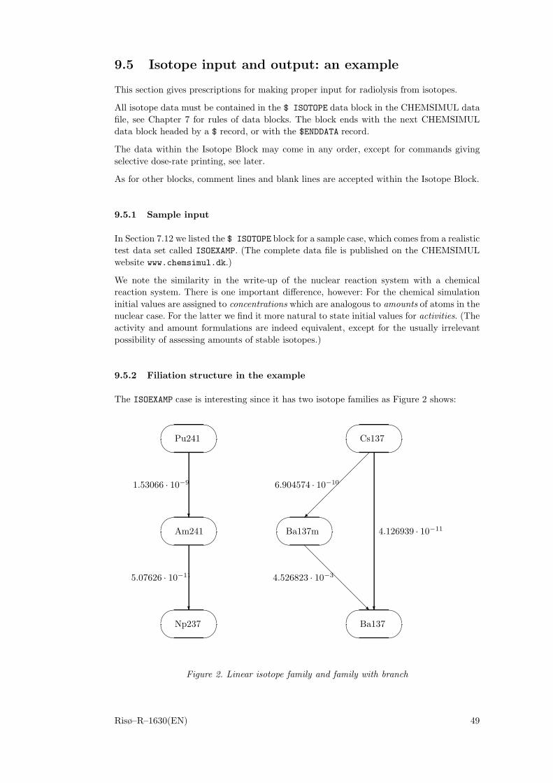
9.5 Isotope input and output: an example

This section gives prescriptions for making proper input for radiolysis from isotopes.

All isotope data must be contained in the $ ISOTOPE data block in the CHEMSIMUL datafile, see Chapter 7 for rules of data blocks. The block ends with the next CHEMSIMULdata block headed by a $ record, or with the $ENDDATA record.

The data within the Isotope Block may come in any order, except for commands givingselective dose-rate printing, see later.

As for other blocks, comment lines and blank lines are accepted within the Isotope Block.

9.5.1 Sample input

In Section 7.12 we listed the $ ISOTOPE block for a sample case, which comes from a realistictest data set called ISOEXAMP. (The complete data file is published on the CHEMSIMULwebsite www.chemsimul.dk.)

We note the similarity in the write-up of the nuclear reaction system with a chemicalreaction system. There is one important difference, however: For the chemical simulationinitial values are assigned to concentrations which are analogous to amounts of atoms in thenuclear case. For the latter we find it more natural to state initial values for activities. (Theactivity and amount formulations are indeed equivalent, except for the usually irrelevantpossibility of assessing amounts of stable isotopes.)

9.5.2 Filiation structure in the example

The ISOEXAMP case is interesting since it has two isotope families as Figure 2 shows:

��

��Pu241

��

��Am241

��

��Np237

��

��Cs137

��

��Ba137m

��

��Ba137

�

�

��

��

��

��

��

��

��

�� �

1.53066 · 10−9

5.07626 · 10−11

6.904574 · 10−10

4.526823 · 10−3

4.126939 · 10−11

Figure 2. Linear isotope family and family with branch

Risø–R–1630(EN) 49

One family is linear, while the other one has a branch. For each decay the correspondingrate constant is shown. We shall see how the $ ISOTOPE block in Section 7.12 encodes thisfiliation structure.

9.5.3 Rules for preparing isotope input

In general the input for the nuclear reactions is given in a way that conforms with (47).Each nuclear reaction equation is prefixed with a unique identification NRn:, where NRmeans Nuclear Reaction and n is the equation identification number. (This syntax is similarto that for the chemical reactions.) Then follows the name chosen for the mother isotope,the character =, and then the name chosen for the daughter isotope followed by a semicolon.Note that isotope names can be chosen freely as alphanumeric text strings; they may beginwith digits, as 243Cm. These names are case sensitive, but otherwise all commands orspecifiers in the Isotope Block are case insensitive.

In the nuclear reaction equation the reaction rate is defined by k=, while the initial doserates for α, β, γ, and neutron irradiation are defined by the 4 terms: DA = ..., DB = ...,DG = ..., and DN = .... Thus the specifiers k=, DA=, DB=, DG=, DN= correspond to k, d′α,d′β , d′γ , and d′n in (47). Omitted specifiers are interpreted as zero. The internal order of thespecifiers is immaterial.

The ACTIVITY command specifies initial activities for the isotopes; the syntax is clear fromthe example.

You should notice that several reactions may contribute to the activity of the same isotope.This will happen when branching occurs. In any case you should always state the totalinitial activity for each isotope.

Use of the specifiers DA=, DB=, DG=, or DN=, requires an initial activity for the mother isotope.Activities must not be specified for stable isotopes.

Inputting of the nuclear G-values in (43) is straightforward: We write GA(X), GB(X), GG(X),GN(X) for the nonzero primary yields Gα

s , Gβs , Gγ

s , Gns , for producing a given species X = Xs.

See the sample input in Section 7.12. Negative primary yields correspond to destructionof species. Refreshable parameter input is supported with the same syntax as indicated inSection 7.8 for the radiolytic primary yields. For example you may write GG(H2) = <ggh2and define ggh2 in your RP block.

It is possible to supplement the standard overall dose-rate tables with additional tableswith specific dose-rate contributions from given radiation types (A, B, G, N), and selectedisotopes. Such a table is generated whenever one or more of the commands DOSERATEA,DOSERATEB, DOSERATEG, DOSERATEN, are present. Each of them takes a comma-separatedlist of isotope names as argument. In our example we have two such commands.

We also mention that there is an isotope command DECAYPRINT which causes tables to beprinted of the decaying amounts and activities of all the isotopes. For isotopes with noinitial activity the initial amounts are (arbitrarily) set to zero. This feature may be usefulfor test purposes. (It was not used in the present example.)

Note that nuclear G-values can enter regular expressions (Sections 6.4) as a braced itemwith the same syntax as for the radiolytic G-values, say {GG(H2)}. The same RP restrictionapplies here too, i.e. if you have defined GG(H2) = <ggh2 you cannot write {GG(H2)} in anexpression but should instead use ggh2.

Moreover, the 4 kinds of total doserates by emission type can occur in regular expressions,by writing {DOSERATEA}, {DOSERATEB}, {DOSERATEG}, or {DOSERATEN}. Such an item willcontain the value of the specific kind of doserate, summed over isotopes, at the actual time

50 Risø–R–1630(EN)

t of the simulation.

9.5.4 Sample output

Here we show the isotope part of the CHEMSIMUL result file for our sample case ISOEXAMP.(To save space not all the table contents are shown here.) We begin with the input-echopart:

=================== INPUT DATA: ISOTOPES ==================

NUCLEAR REACTION SYSTEM-----------------------NR1:Pu241=Am241;k=1.53066E-9,DB=2.80E-11NR2:Am241=Np237;k=5.07626E-11,DA=4.12E-5,DG=1.70E-9NR3:Cs137=Ba137m;k=6.904574E-10,DB=6.29E-5NR4:Cs137=Ba137;k=4.126939E-11,DB=8.98E-6NR5:Ba137m=Ba137;k=4.526823E-3,DG=2.15E-4

INITIAL ACTIVITIES------------------ACTIVITY(Pu241)=5.2E12ACTIVITY(Am241)=5.0E10ACTIVITY(Cs137)=1.755E13ACTIVITY(Ba137m)=1.755E13

PRIMARY YIELDS--------------SPECIES A B G NE[-] 0.060000 2.660000 2.660000OH[-] 0.100000 0.100000OH 0.240000 2.670000 2.670000H2O -2.710000 -6.970000 -6.970000H2O2 0.985000 0.720000 0.720000HO2 0.220000H 0.210000 0.550000 0.550000H2 1.300000 0.450000 0.450000H[+] 0.060000 2.760000 2.760000

NO. OF NUCLEAR REACTIONS = 5NO. OF INITIAL ACTIVITIES = 4NO. OF ISOTOPES = 6

In the result file you will find two standard tables of accumulated doses as well as doserates, originating from the decaying isotopes. These tables look as follows:

================= OUTPUT TABLES: ISOTOPES =================

ACCUMULATED DOSES FROM ISOTOPES------------------------------------------------------------------------

TIME A B G N TOTAL0.0000E+00 0.0000E+00 0.0000E+00 0.0000E+00 0.0000E+00 0.0000E+003.1558E+10 2.8640E+06 9.8233E+04 2.7737E+05 0.0000E+00 3.2396E+066.3115E+10 3.4604E+06 9.8233E+04 2.7740E+05 0.0000E+00 3.8360E+06

Risø–R–1630(EN) 51

...2.5246E+11 3.6109E+06 9.8233E+04 2.7740E+05 0.0000E+00 3.9866E+062.8402E+11 3.6109E+06 9.8233E+04 2.7740E+05 0.0000E+00 3.9866E+063.1558E+11 3.6109E+06 9.8233E+04 2.7740E+05 0.0000E+00 3.9866E+06

DOSE RATES FROM ISOTOPES------------------------------------------------------------------------

TIME A B G N TOTAL0.0000E+00 4.1200E-05 7.1880E-05 2.1500E-04 0.0000E+00 3.2808E-043.1558E+10 3.7918E-05 6.7310E-15 1.5646E-09 0.0000E+00 3.7920E-056.3115E+10 7.6406E-06 6.3030E-25 3.1527E-10 0.0000E+00 7.6409E-06...2.5246E+11 5.1148E-10 4.2499E-85 2.1105E-14 0.0000E+00 5.1150E-102.8402E+11 1.0307E-10 3.9797E-95 4.2527E-15 0.0000E+00 1.0307E-103.1558E+11 2.0768E-11 0.0000E+00 8.5694E-16 0.0000E+00 2.0769E-11

Because it was requested in the input, there will also appear a selective dose-rate table:

SELECTIVE DOSE RATES BY TYPE AND ISOTOPE----------------------------------------

TIME DB(Pu241) DA(Am241)0.0000E+00 2.8000E-11 4.1200E-053.1558E+10 2.9445E-32 3.7918E-056.3115E+10 3.0965E-53 7.6406E-06...2.5246E+11 0.0000E+00 5.1148E-102.8402E+11 0.0000E+00 1.0307E-103.1558E+11 0.0000E+00 2.0768E-11

9.5.5 Saving isotope results for manual restart

As outlined in Section 7.15 it is possible to store chemical concentration values at t = tend ina save file, by using the SAVE command. This save facility extends to isotopic data wheneveran Isotope Block is present, thus admitting an easy way to make “manual restarts” alsowhen isotopes are involved. To ensure data integrity and easy copying, CHEMSIMUL insertsa complete revised Isotope Block at the end of the save file, as the small example belowshows. We suppose that a data file contains SAVE and has the following Isotope Block:

$ISOTOPESNR1: I1 = XXX; K=0.00693, DA=1, DG=1 ! Period = 100NR2: I2 = XXX; K=0.00347, DA=1, DG=1 ! Period = 200GG(OH)=2.67...GA(H2O)=-5.46ACTIVITY(I1)=0.00693ACTIVITY(I2)=0.00347

Then, at the end of simulation, a save file with a revised Isotope Block is created:

...CON(MH2OH2) = 2.1591181174106500E-05****** ISOTOPE BLOCK INTENDED TO REPLACE PREVIOUS BLOCK BEFORE RESTART:

52 Risø–R–1630(EN)

$ISOTOPESNR1:I1=XXX; K=0.00693, DA= 5.00073596E-01, DG= 5.00073596E-01NR2:I2=XXX; K=0.00347, DA= 7.06805328E-01, DG= 7.06805328E-01GG(OH)=2.67...GA(H2O)=-5.46ACTIVITY(I1) = 3.46551002E-03ACTIVITY(I2) = 2.45261449E-03****** ENDSAVE ... END OF SAVE FILE

By comparing this with the input file you will notice that the dose coefficients DA=... etc.,as well as the activities are replaced by end simulation values, while the remaining IsotopeBlock is left intact. You may then copy the block as a whole into an input file and let itreplace the Isotope Block there.

10 Ionic strength calculations

The ionic strength is a parameter which characterizes the ionic contents of aqueous solu-tions. As a consequence of ionic strength, rate constants between two charged reactantsmay be altered. This salt effect is important in the theory of electrolytes. CHEMSIMULhas no direct procedures for computing the quantities mentioned in this chapter, and it hasno particular data block for ionic strength. Instead the program offers a number of toolsfor easing your simulation work when this involves ionic strength. Refreshable parameters(RPs) play an important role in such calculations.

10.1 Ionic strength definitions

First we give the definition of ionic strength based on conventional volumetric units:

I =12

∑i

CXiz2Xi

(48)

where CXi is the molarity concentration (mol/dm3 solution) of ion Xi, zXi is the chargeof that ion (positive or negative), and the sum is taken over all ions in the solution. Fora 1:1 electrolyte such as sodium chloride, the ionic strength is equal to the concentration.For multivalent ions, the ionic strength is greater than the concentration. I is measured inmol/dm3.

However, for a more accurate estimation of the salt effect it is better to replace (48) withthe following formula:

I∗ =12

∑i

AXiz2Xi

(49)

This differs from (48) in the term AXi , which is the molality concentration (mol/kg solvent)of ion Xi, cf. Section 2.9. (To discern the two, I is sometimes called the pseudo ionic strengthand I∗ the true ionic strength.) If we substitute (14) from Section 2.9 in (49) we obtain thesimple conversion formula

I∗ =I

CUC(50)

where CUC was defined in (13) in Section 2.9. I∗ is measured in mol/kg.

Risø–R–1630(EN) 53

10.2 Activity and Davies’ formula

Activity is a concept involved in various problems such as pH calculation, chemical equi-libria, solubility, etc. The specific definitions of activity and activity coefficients depend oncontext. Here we shall just give a couple of examples. First, the activity of water is givenby the formula

ActH2O =CH2O

CH2O +∑

CXi

(51)

where CH2O is the concentration of water, while CXi is the concentration of solute Xi, bothgiven as molarities. Next we shall give the formula for an activity coefficient γ, which is themain application of ionic strength. For a species X with charge zX this can be calculatedfrom:

log10 γ = −0.5092× z2X

( √I∗

1 +√

I∗− 0.3I∗

)(52)

This formula is based on the Debye-Huckel model with the modification of Davies whoproposed the correction −0.3I∗. It is therefore called Davies’ formula.

An important kinetic application of (52) is to estimate the rate constant k under influenceof the salt effect. The resulting expression becomes

log10

( k

k0

)= 1.0184 zAzB

( √I∗

1 +√

I∗− 0.3I∗

)(53)

or, equivalently,k = k0 × 101.0184 zAzB (

√I∗/(1+

√I∗)−0.3I∗) (54)

Here k is the rate constant at the ionic strength I∗, and k0 the rate constant at the ionicstrength zero. The numbers zA and zB are the charges of the two reactants. For example,we have zA = −1 and zB = 2 in the following reaction:

S− + T++ = S + T+ (55)

The expression (53) corresponds to the original Brønsted-Bjerrum relation for the salteffect, except for Davies’ correction −0.3I∗ [12, 13].

When ionic strength is applied to compute activity or kinetic corrections, as in (52) and(53), the maximum ionic strength compatible with the model is about 0.5 mol/kg; in moregeneral applications this limit will be about 0.3 mol/kg.

10.3 Ionic strength with CHEMSIMUL

We shall now describe how the quantities in Sections 10.1 and 10.2 can be calculated inCHEMSIMUL by means of predefined refreshable parameters (RP). These include ION for I

in (48), SIGMACi for∑

i CXi in (51), and SIGMAMiCi for∑

i MXiCXi in (13) in Section 2.9.Note that the sums SIGMACi and SIGMAMiCi exclude the solvent H2O. To ensure thatCHEMSIMUL makes this exclusion properly, you must use the species name H2O (uppercase) for water.

Observe also that CHEMSIMUL extracts the charges zXi of species Xi from their names,in order to compute I in (48). You must therefore provide proper square bracket qualifiersof the species names, e.g. CO3[--], cf. the naming rules for CHEMSIMUL species given inSection 6.3.

We give below an example to explain the use of the ionic strength features, where we showan excerpt of the data file for a simulation case with carbonation of pure water. We beginby listing part of the $ CHEMICAL REACTIONS block:

54 Risø–R–1630(EN)

$ CHEMICAL REACTIONS* Water equilibrium H2O/OH[-], pKe = 13,9953RE67:H2O+H2O=OH[-]+H3O[+];A=<k67RE68:OH[-]+H3O[+]=H2O+H2O;A=1.103078125E11...

Besides water the total system contains 6 species called OH[-], H3O[+], HCO3[-], CO3[--],CO2, and H2CO3. In order to activate the ionic strength facilities you should put the commandIONIC in the $ MISCELLANEOUS block:

$ MISCELLANEOUS...ionic

Without this command CHEMSIMUL will not establish the predefined parameters men-tioned above. In the $ SYMBOLIC CONSTANTS block you put the molar masses (kg/mol) forall the solute species as follows (including a couple of other constants):

$ SYMBOLIC CONSTANTS...* Molar Masses (kg/mol)# MMOH[-]=17.00734E-3# MMH3O[+]=19.02322E-3# MMHCO3[-]=61.01714E-3# MMCO3[--]=60.0092E-3# MMCO2=44.0098E-3# MMH2CO3=62.02508E-3...# RHOw=996.999 ! Density of water (kg/m3)# Kw=1.0108470836822549E-14 ! Water dissociation constant...

The full species name should be immediately preceded by MM (upper case). As a result,CHEMSIMUL generates an internal RP called SIGMAMiCi. This can be used in the sameway as the “normal” RPs defined in the $ REFRESHABLE PARAMETERS block, i.e. it worksexactly as an RP defined by

<SIGMAMiCi = MMOH[-] * OH[-] + ... + MMH2CO3 * H2CO3

CHEMSIMUL will not generate SIGMAMiCi if some molar masses are missing, or none arepresent at all, but it will still generate ION and SIGMACi. This might be OK for you, if youdo not intend to work with molalities. On the other hand, the presence of molar masses forspecies that are not in the reaction system, will do no harm; you may for example wish tohave a “library” of molar masses placed in your $ SYMBOLIC CONSTANTS block.

Proceeding now to the $ REFRESHABLE PARAMETERS block, we see several essential simula-tion quantities being formulated here:

$ REFRESHABLE PARAMETERS* RPs SIGMAMiCi, SIGMACi, ION automatically generated by CHEMSIMUL< RHOLIQ=RHOw/2+104.673*SQRT(SIGMAMiCi+2.281766E-5*RHOw^2) ! Density< CUC=1E-3*RHOLIQ-SIGMAMiCi ! Conversion of Unit of Concentration< IS=ION/CUC ! Conversion into true ionic strength< gamma=10^(-0.5092*(SQRT(IS)/(1+SQRT(IS))-0.3*IS)) ! Act.coeff.(Davies)

Risø–R–1630(EN) 55

* Water equilibrium:< ActH2O=H2O/(H2O+SIGMACi) ! Activity of water< k67=1.103078125E11*Kw*(H2O*CUC/(gamma*ActH2O))^2 ! feedback to RE67...

In summary, you must formulate your ionic strength model yourself, but CHEMSIMULprovides facilities to reduce your work with this.

11 Hints for special problems

Although many simulation problems in chemical kinetics at first sight do not appear to bedirectly solvable by CHEMSIMUL, a reformulation of the original problem may sometimeshelp. In this chapter you will find a number of hints which enable you to solve such specialproblems with the program.

11.1 How to mark a reaction

If you want to know how much material is passing through a single reaction you can markthe reaction without sacrificing the material balance: The reaction

RE1: A + B = C + D; A =k1 (56)

is marked like this:RE1: A + B = AB; A =k1 (57)

RE2: AB + M = C + D + N; A =k2 (58)

CON(M) = M (59)

To ensure that RE1 is rate determining during the whole simulation you must choose highvalues for M and k2:

M × [AB] × k2 � [A] × [B] × k1 (60)

The simulated concentration [N] represents the yield of this reaction.

11.2 Maintain constant concentration of solute

The program is designed to preserve the mass balance. In view of this you may use eitherof two possible methods, if you want to maintain a constant concentration for a solute X:

11.2.1 The equilibrium method

Here you assign a high initial concentration M to a DUMMY species in equilibrium with X:

CON(DUMMY) = M (61)

RE1: DUMMY = X; A =a (62)

RE2: X = DUMMY; A =b (63)

Choose a value for the rate constant a (e.g. 100) and calculate b from the equation:

M × a = [X] × b (64)

M must be so high that the change in concentration during the simulation is insignificant.

56 Risø–R–1630(EN)

11.2.2 The conservation method

This method recreates X whenever X is consumed in a reaction, and removes X whenever Xis produced in a reaction. As an example consider the reactions:

RE1: X + N = X[−] + N[+]; A =a

RE2: C + B = X + D; A =b (65)

Assign a high DUMMY concentration as in (61). Change the equations as follows:

RE1: X + N = X[−] + XN[+]; A =a

RE2: C + B = DUMMY+ D; A =b (66)

and add the reactionRE3: XN[+] + DUMMY = X + N[+]; A =c (67)

Choose the rate constant c so high that X is produced much faster in RE3 than it is consumedin RE1.

11.3 Equilibrium of gas phase with solution

If you have a gas phase (volume = g) in equilibrium with a liquid phase (volume = �) andyou want to maintain the equilibrium of for example oxygen during the simulation, thiscan be accomplished in the following way:

First determine the equilibrium concentration ratio of dissolved oxygen O2 and gas phaseoxygen O2,gas:

[O2][O2,gas]

= r (68)

Then introduce a DUMMY species whose concentration [DUMMY] is calculated as the oxygenconcentration if the gas phase had the same volume as the liquid phase:

[DUMMY] = [O2] × g

�(69)

Finally determine the rate constants a and b in the equilibrium reactions

RE1: DUMMY = O2; A =a (70)

RE2: O2 = DUMMY; A =b (71)

by first choosing a value for a (e.g. 100) and then calculating b from the equation:

[DUMMY] × a = [O2] × b (72)

11.4 Mass balance for G-values

CHEMSIMUL does not check the mass balance for the G-values. The reason is that eachspecies name is an indivisible entity with no possibility of analysing its atomic contents. (Itis an important feature in CHEMSIMUL that names can be chosen freely, especially whenorganic molecules are involved.)

In case of water irradiation it is possible to preserve the mass balance, if you make surethat the following 3 equations are fulfilled:

1. Hydrogen balance:

2G(H2O) + G(H) + G(H[+]) + G(OH) + G(HO2) + 2G(H2) + 2G(H2O2) + G(OH[−]) = 0 (73)

Risø–R–1630(EN) 57

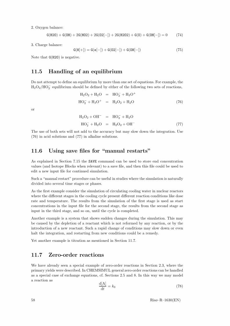
2. Oxygen balance:

G(H2O) + G(OH) + 2G(HO2) + 2G(O2[−]) + 2G(H2O2) + G(O) + G(OH[−]) = 0 (74)

3. Charge balance:G(H[+]) = G(e[−]) + G(O2[−]) + G(OH[−]) (75)

Note that G(H2O) is negative.

11.5 Handling of an equilibrium

Do not attempt to define an equilibrium by more than one set of equations. For example, theH2O2/HO−

2 equilibrium should be defined by either of the following two sets of reactions,

H2O2 + H2O = HO−2 + H3O+

HO−2 + H3O+ = H2O2 + H2O (76)

or

H2O2 + OH− = HO−2 + H2O

HO−2 + H2O = H2O2 + OH− (77)

The use of both sets will not add to the accuracy but may slow down the integration. Use(76) in acid solutions and (77) in alkaline solutions.

11.6 Using save files for “manual restarts”

As explained in Section 7.15 the SAVE command can be used to store end concentrationvalues (and Isotope Blocks when relevant) to a save file, and then this file could be used toedit a new input file for continued simulation.

Such a “manual restart” procedure can be useful in studies where the simulation is naturallydivided into several time stages or phases.

As the first example consider the simulation of circulating cooling water in nuclear reactorswhere the different stages in the cooling cycle present different reaction conditions like doserate and temperature. The results from the simulation of the first stage is used as startconcentrations in the input file for the second stage, the results from the second stage asinput in the third stage, and so on, until the cycle is completed.

Another example is a system that shows sudden changes during the simulation. This maybe caused by the depletion of a reactant which is not reformed by any reaction, or by theintroduction of a new reactant. Such a rapid change of conditions may slow down or evenhalt the integration, and restarting from new conditions could be a remedy.

Yet another example is titration as mentioned in Section 11.7.

11.7 Zero-order reactions

We have already seen a special example of zero-order reactions in Section 2.3, where theprimary yields were described. In CHEMSIMUL general zero-order reactions can be handledas a special case of exchange equations, cf. Sections 2.5 and 8. In this way we may modela reaction as

d[A]dt

= k0 (78)

58 Risø–R–1630(EN)

where k0 is a constant. When setting up the differential equation for the species A, CHEM-SIMUL will then add k0 to the right-hand side.

Zero-order reactions can be used for simulation of constant-rate addition of a reactant tothe reaction system (titration). The setting of start and end time of the titration can befacilitated by means of the SAVE command in CHEMSIMUL.

Catalytic reactions can also be described by zero-order reactions. For example, the catalyticdecomposition of H2O2 can be described by 3 zero-order reactions.

11.8 Third body reactions

Reactions of higher order than 2 should not be considered in condensed phase, and thepresent version of CHEMSIMUL does not accept reactions of higher order. However, in gasphase many reaction rates are dependent on a “third body” M to absorb surplus reactionenergy, as in the reactions

A + B + M → P + M (79)

andA + M → C + D + M (80)

with rate constants k1 and k2, respectively. These reactions are formally third and secondorder reactions, but actually they are pseudo-second and pseudo-first order, respectively,because the concentration [M] does not change during the reaction. This means that thedifferential equation for the third-order reaction

d[P]dt

= k1[A][B][M] (81)

can be reduced tod[P]dt

= kM[A][B] (82)

wherekM = k1[M] (83)

To be acceptable for CHEMSIMUL the reactions (79) and (80) must be presented in thefollowing form:

A + B → P (84)

andA → C + D (85)

These reactions should be assigned the rate constants k1 × [M] and k2 × [M], respectively.

Another option would be to express (81–83) in terms of exchange equations (Chapter 8).

12 Simulation examples

Rasmussen and Bjergbakke [1] gave several examples of simulations using an earlier ver-sion of CHEMSIMUL. Their examples spanned from dosimetry and NOx processes in theatmosphere to the study of radiolysis of ground water from spent nuclear fuel. They alsosimulated classical processes, notably the Belousov-Zhabotinskii oscillating reaction, whichhas gained renewed interest as a chemical example of a dynamic system with the typicalnonlinear features of limit cycles, period doubling, and eventually chaos.

Here we shall only illustrate two of these test runs with graphical output obtained withCHEMSIMUL plot expressions. Details for these examples are found in Rasmussen andBjergbakke [1].

Risø–R–1630(EN) 59

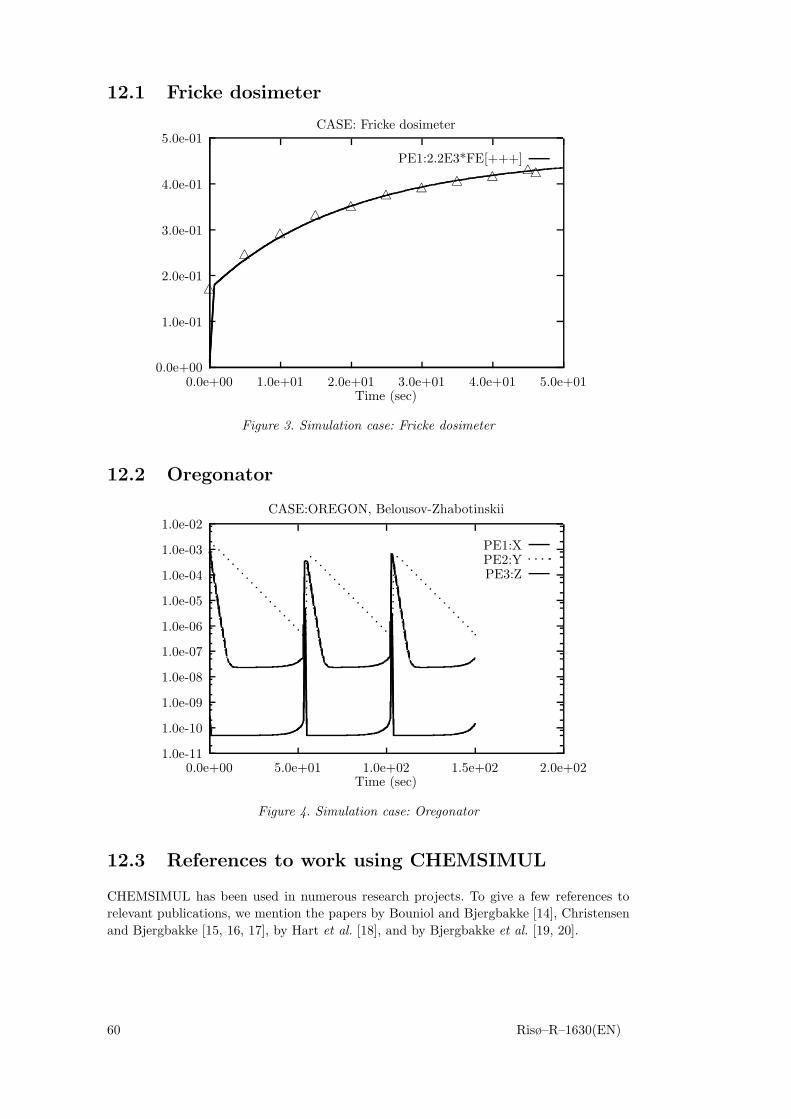
12.1 Fricke dosimeter

0.0e+00

1.0e-01

2.0e-01

3.0e-01

4.0e-01

5.0e-01

0.0e+00 1.0e+01 2.0e+01 3.0e+01 4.0e+01 5.0e+01Time (sec)

CASE: Fricke dosimeter

PE1:2.2E3*FE[+++]�

�

��

� � � � � � �

Figure 3. Simulation case: Fricke dosimeter

12.2 Oregonator

1.0e-11

1.0e-10

1.0e-09

1.0e-08

1.0e-07

1.0e-06

1.0e-05

1.0e-04

1.0e-03

1.0e-02

0.0e+00 5.0e+01 1.0e+02 1.5e+02 2.0e+02Time (sec)

CASE:OREGON, Belousov-Zhabotinskii

PE1:XPE2:YPE3:Z

Figure 4. Simulation case: Oregonator

12.3 References to work using CHEMSIMUL

CHEMSIMUL has been used in numerous research projects. To give a few references torelevant publications, we mention the papers by Bouniol and Bjergbakke [14], Christensenand Bjergbakke [15, 16, 17], by Hart et al. [18], and by Bjergbakke et al. [19, 20].

60 Risø–R–1630(EN)

13 Mathematical details

In the following we shall discuss the principal features in the mathematical implementa-tion of the CHEMSIMUL program. Readers without special interest for the CHEMSIMULmathematics may skip this chapter.

13.1 Translation principle for reactions

To explain the mechanism of the CHEMSIMUL translator, let us assume a general chemicalsystem being specified with M reactions involving altogether N species. We write thereaction system in the following way:

Reac(r) : αj × Rj + αk × Rk →∑

α� × R�, r = 1, . . . , M (86)

where Rs is the chemical symbol for species s, s = 1, . . . , N . The left-hand side is emptyfor a zero-order reaction. Otherwise αj , αk, α� are non-negative integers satisfying 1 ≤αj + αk ≤ 2. For a second-order reaction we may have j = k or j = k; in both casesαj + αk = 2. Each reaction Reac(r) is assigned a rate constant kr. Moving the reactantterms in (86) to the right-hand side, we may assign with every species s in reaction r astoichiometric coefficient ars, which is positive for a product and negative for a reactant.Setting unassigned entries ars = 0, we obtain the stoichiometric matrix A = (ars) ∈ �M×N.This enables us to express the reaction system in compact vector-matrix notation as

Av = 0 (87)

where the entries of the N -dimensional species vector v ∈ SN are the species names Rs inthe symbol set S for the reaction system. The resulting general ODE system for the speciesconcentrations has the form

d[Rs]dt

=∑j,k

njksMjks[Rj ][Rk] +∑

j

njsMjs[Rj ] + c GsD′(t), s = 1, . . . , N (88)

The right-hand side of (88) is the sum of a quadratic form coming from the second-orderreactions, a linear form from the first-order reactions, and a term coming from the zero-orderreactions. The 3-dimensional tensors njks and Mjks contain the stoichiometric coefficientsars and the reaction rates kr, respectively. For a given s, the sum is taken over pairs (j, k)for which (Rj , Rk) is a reacting pair in some reaction r = r(j, k) involving Rs on eitherside, with njks = ars and Mjks = kr. A similar interpretation holds for the linear form. Forsimplicity we here assume that the zero-order term has the form c GsD

′(t), where c is theconversion factor, Gs the G-value for species s, and D′(t) the dose rate at time t. (In caseof irradiation from decaying isotopes the zero-order term is given by the right-hand side of(43).)

Given a computerized write-up like (25) of the reactions (86), CHEMSIMUL assembles theODE system (26) or (88) from all the individual pieces in the reactions. On encounter ittabulates every new species and includes its name in the symbol set S. It also stores therate constants kr. After the scan phase an assembly phase is invoked. Here CHEMSIMULconstructs a matrix with 5 rows and one column for each second-order or first-order term onthe right-hand side of the total ODE system. Entry 2 in the column contains the stoichio-metric coefficients njks, while the other entries contain address pointers to 1) the species s,3) the reaction r, 4) [Rj ], and 5) [Rk] (for first-order processes we may set [Rk] = 1). Thispointer table gives a complete description of the ODE system and permits the evaluationof its Jacobian.

Risø–R–1630(EN) 61

13.2 Balance check by linear programming

The accurate solution of the ODE system in chemical kinetics requires an overall con-servation of the mass balance, as pointed out by Ridler et al. [21]. This balance may beaffected by two main factors, the reaction mechanism and the integration process. Beinga linear multistep method, the numerical integration scheme in CHEMSIMUL has the im-plicit property of mass preservation, as shown by Rosenbaum [22, 23]. Hence it is sufficientto make a static consistency check, and as stated in Section 5.1, such a check should bebased on the demand of existence of strictly positive solutions to the balance equation (28)or (87) where A is the stoichiometric matrix and v the species vector.

Ridler et al. [21] proposed a heuristic checking method based on Gaussian elimination ininteger arithmetic on A, and that method was adopted by Rasmussen and Bjergbakke in[1]. Later we replaced it by a mathematically more stringent method: By the homogeneityof (87) we can replace the demand of positive values by a demand of all values be ≥ 1.Thus, if A = (aij), it must be possible to find solutions yj ≥ 1 to the equations

N∑j=1

aijyj = 0, i = 1, . . . , M (89)

On writing yj = xj + 1 we may replace (89) by the system

Ax = b, x ≥ 0 (90)

where x = (xj) and b = (bi) with bi = −∑Nj=1 aij . To decide the feasibility of (90) is a

standard linear-programming problem. It can be solved efficiently by the simplex method.

13.3 Solution of the ODE system

A system of ordinary differential equations is conveniently expressed in vector notation:

dy

dt= f(y, t) (91)

The ODE systems in chemical kinetics are typically non-linear and autonomous,

f(y, t) = f (y) (92)

As mentioned in Section 1.3 the corresponding initial-value problems may be of the stifftype. After many years of experience we are still in favor of using the DLSODA solverfrom Hindmarsh’ ODEPACK collection, written by Petzold [4] and Hindmarsh [5]. Thiscode (originally named LSODA) switches automatically between stiff and nonstiff methods,starting with a nonstiff (Adams) method.

When the stiff BDF procedure is invoked (BDF = Backward Difference Formula), theJacobian df/dy will be needed. This can be supplied by CHEMSIMUL or estimated byDLSODA, cf. Section 13.4.

DLSODA admits a combined relative and absolute error control: It controls the vectore = (ei) of estimated local errors in the solution y = (yi) by the restriction ‖r‖∞ ≤ 1,where r = (ri) is given by ri = ei/wi with wi = εreli |yi| + εabs

i . Thus each component ei ofthe local error must satisfy

ei ≤ εrel|yi| + εabsi (93)

Normally CHEMSIMUL will not need this flexibility; usually fixed relative and absolutetolerances εreli = εrel and εabs

i = εabs, ∀i, give good results in practice, and this correspondsto the present implementation.

In radiolytic simulations, where the irradiation burst induces a constant source term in thefinite time slot [0, tr] and then disappears, we found that the best way of using the solver

62 Risø–R–1630(EN)

was to select the one-step mode in combination with a critical time barrier t = tr (ITASK= 5 in DLSODA). Integration beyond the discontinuity point tr proceeds ab initio fromt = tr. The same technique is used for a pulse train. Thus the simulation is partitioned intoa number of smooth subproblems.

The one-step mode is also convenient when producing result tables for printing and plotting.Whenever a new printing time tp is surpassed by the current integration time t, the resultsat tp are computed by an interpolation routine provided by DLSODA, cf. Section 13.6. Asfor the graphics tables, a plotting time mesh is constructed beforehand, either linear orlogarithmic, and each time the integration time t enters a new plotting mesh, a plottingpoint (t, y) will be recorded.

There are a number of useful tools and options in DLSODA. It is possible to specify a min-imum step length hmin (not implemented in the present CHEMSIMUL version). It is alsopossible to prescribe a maximum step length hmax, and an initial step length h0 to be at-tempted instead of the internally computed default value. In the applications we sometimesmeet quite hard kinetics problems, where for instance a species approaches zero concentra-tion very rapidly. Here we may see traces of instability with negative concentrations, andeven break-down of the integration procedure. A very successful standard remedy for suchtroublesome cases is to reduce one or more of the parameters in the triple (εrel, hmax, h0).

13.4 The Jacobian

When DLSODA switches to its stiff integration procedure, it will need the Jacobian df/dy

of the right hand side of the ODE system (91). This is a square matrix whose order m

equals the dimension of y.

The Jacobian needs not to be exact in order to get DLSODA working properly. A fairapproximation will do. However, a bad Jacobian approximation may have a devastatinginfluence on the computing time, or even halt the simulation with an integration failure.

There are several ways in which the Jacobian can be supplied. The actual choice is governedby the command JT = ... (Section 7.6), as outlined in Table 5:

JT value Kinetics part Exchange part1 Analytic expressions Numerical estimate

(default) by CHEMSIMUL by CHEMSIMUL2 Numerical estimate Numerical estimate

by DLSODA by DLSODA3 Analytic expressions Contribution

by CHEMSIMUL ignored

Table 5: Choices for Jacobian evaluation

The numerical estimates are provided by difference quotient approximations.

If the system is dominated by purely kinetic equations (and possibly temperature), withno or few exchange equations (Section 2.5), experience shows that it is best to supply ananalytical Jacobian. Since df/dy is then simple and cheap to calculate exactly, this willnormally give a faster integration with less risk of error stops.

Many problems require that the Jacobian contribution from the exchange equations is takeninto account, in order to make the integration proceed at a reasonable speed. This is whywe have made JT = 1 the default option in CHEMSIMUL.

In other problems the exchange equations have little influence on the Jacobian, and itscontribution may safely be ignored. For such cases JT = 3 is available.

Risø–R–1630(EN) 63

Only in rare cases JT = 2 should be used. The reason is that the numerical estimation ofderivatives in the kinetics part will slow down the calculations, in particular in systemswith many chemical reactions.

Contribution to the Jacobian from refreshable parameters are ignored unless JT = 2. Thisapproximation is tolerable since RPs are normally slowly varying with time.

In the following we present the proper formulas for the Jacobian elements in the analyticalcases JT = 1 and JT = 3, assuming first that the vector y contains concentrations only. Inthat case m = N , i.e. the number of species, and it is easy to compute df/dy from (88);see also the ODE system (26) for our sample case. We find for the (s, k)-element:(df

dy

)sk

=∑

j

(njksMjks + nkjsMkjs)[Rj ] + nksMks (94)

For the interpretation of the j-sum, see similar comments in Section 13.1.

Incorporation of the adiabatic process described in Section 2.7 induces an augmentation ofthe Jacobian with one extra row and column, such that now m = N + 1. Row and columnm refer to the temperature T . Let us first consider column m. This will be nonzero if thereis a temperature dependence in some of the reaction rates kr = k(T ). For example, withthe modified Arrhenius form (5) we find

∂k

∂T= AT β exp(−Ea/(RT ))

(β

T+

Ea

RT 2

)(95)

Practical experience shows that (95) has negligible influence on the behavior of the numeri-cal integration. The same can be expected when k(T ) is determined by tabular interpolation.In these cases the influence from temperature on the parameters is usually much weakerthan that coming from the reaction rates. Consequently we can safely set the entire columnm to zero. Let us then consider row m. Here we find from (8–9):

(df

dy

)m�

=1

S2cap

(( M∑r=1

krqr(δj�[Rk] + δk�[Rj ]))Scap − Q′(t)cv(R�)

), � = 1, . . . , N (96)

where Scap is the denominator of (8), and δij is the Kronecker delta. The species indicesj = j(r) and k = k(r) depend on the reaction r; for first-order reactions r the correspondingsummand in (96) should read krqrδj�.

The dose terms in (88) or (43) bear no influence on the Jacobian.

13.5 Computation of derivatives

Derivatives may be requested either in the result table by the command DERIVATIVE or aspart of a plot expression by the syntax S’. It is well known that it is harder to compute fairapproximations to the derivative of a quantity in a numerical simulation, than to computethe quantity itself. In this respect CHEMSIMUL is no exception. In principle, we maycompute d[S]/dt in two ways:

– Method I: Direct evaluation from the kinetics equation for the species:

d[S]dt

= RHS (97)

where RHS usually contains positive and negative terms involving concentrations andrate constants of S and the other species that affect the build-up or decay of S. (Anexample of kinetics equations was presented in the write-up (26) in Section 3.2.)

– Method II: By numerical estimation from the simulated curve [S](t) produced byCHEMSIMUL either as a result table or preferably a plot table. This may be done byusing symmetric difference-quotient approximations to the derivatives.

64 Risø–R–1630(EN)

Both methods have advantages and drawbacks. Method I is readily implemented, as thekinetics equations are needed anyway in the simulation. It gives a “snapshot” computationof d[S]/dt at current time. In the majority of cases it is more accurate than Method II.However, it occasionally breaks down completely, in particular when S is an intermediatelow-concentration species. It may then happen that RHS in (97) becomes the differencebetween very large contributions from dominant species. If CHEMSIMUL calculates thelatter to a relative precision of say εrel = 10−3, all precision may get lost by cancellation sothat d[S]/dt will contain numerical noise only.

Although Method II is usually less accurate it is more robust in extreme situations. It mayseem a paradox that taking quotient differences in the solution curve could really be betterthan using the kinetics equations directly; after all the latter equations are the basic inputfor the ODE solution. The paradox is partly resolved by considering that DLSODA usesadvanced techniques with good stability and conservation properties, and stores importantinformation on the behaviour of the solution in a neighbourhood of the current simulationtime. This admits a reasonable computation even of the less significant species.

CHEMSIMUL uses Method I for derivatives in result tables, and Method II for derivativesin plot expressions.

13.6 Interpolation techniques

Various kinds of interpolation techniques are used in CHEMSIMUL. For interpolation inthe user-specified tables (Sections 7.14.2 and 7.14.3) we use cubic splines. There are severalvariants of such splines. The natural spline is characterized by vanishing second derivativesat the end points T1 and Tn. We prefer however the Moler spline [11], where the thirdderivative in T1 matches that of the unique cubic through T1, T2, T3, and T4 and similarlyat the other end.

Prediction of maximum concentrations and correponding time postions (Section 5.3) isfacilitated by parabolic interpolation over 3 points picked from the “plot table” which iscalculated during integration. This parabola corresponds to the Lagrangian polynomial forthe 3 points.

Also the DLSODA integrator [4, 5] uses interpolation. This is based on the so-called Nord-sieck history array.

13.7 Implementation of regular expressions

When describing the implementation of regular expressions (cf. Section 6.4) we use a plotexpression example:

PE1: 4711.77 + (log10(OH[-])/7.45)^1.5 (98)

The interpretation of such an expression has two phases, a lexicographical analysis and asuccessive processing. The lexicographical analysis decomposes the plot expression into alist of atoms. Each atom is a constant, a species name, an arithmetic operator, or a functionname. The 7 possible operators are those of elementary algebra: ∗, /, +, −, ^, (, and ), where^ stands for exponentiation; depending on context + and − can be infix or unary. The 10standard mathematical functions cos, cosh, exp, ln, log10, sin, sinh, √ , tan, and tanh aresupported. The string of atoms is ended with an “empty atom”, which is considered as anextra operator. In the above example we get the atom list shown in Table 6, where speciesare supposed to be assigned definite concentration values:

Risø–R–1630(EN) 65

Atom# Atom Type1 4711.77 Constant2 + Operator3 ( Operator4 log10 Function5 ( Operator6 OH[-] Species7 ) Operator8 / Operator9 7.45 Constant10 ) Operator11 ^ Operator12 1.5 Constant13 empty Operator

Table 6. Atoms in a plot expression

We process this table atom by atom using common techniques from computer science: Wecreate and maintain two stacks V and O, the first for values (operands) and the secondfor operators. Moreover we use a separate stack F for the mathematical function names.Functions are considered as unary operators of highest priority with the common classname ”f”.

An operand may be a constant, a concentration value, or a computation result. A newoperand always pushes V and enters its top.

Let N be a new operator and T the current top-of-stack operator. If N = ”(”∨N = ”f”, N

pushes O and enters its top; when N = ”f” it also pushes F. Otherwise we continue fromthe algorithmic point called A: If |O| = 0, N pushes O. But if |O| > 0 we observe whetherT = ”(”∧N = ”)”. If so, T is devoured and O is popped. If not we continue by comparingpriorities π: If π(N) ≤ π(T ), a unary or binary operation takes place on the current topvalue(s). If T = ”f”, a function call is executed followed by popping the function stack;if T is unary + or − the corresponding operation takes place; otherwise we have a binaryoperation with T = +, −, ∗, /, or ^. After the operation O is popped, while the top valueis updated with the current result. If the operation was binary, V is popped, too. Afterpopping O we go back to point A in the algorithm. If, on the other hand, π(N) > π(T ),then O is pushed, and so is F if N = ”f”. After storing the operator N , a new atom willbe processed.

A small complication arises when repeated exponentiation occurs, since the operation orderis then from right to left: When N = T = ^, we postpone the binary operation simply byletting ^ push O and processing immediately to the next atom.

The algorithm terminates when the empty operator enters the top of O. When this happenswe must have |V| = 1.

We use the following operator priority list (from low to high):

{empty}, {( , )} {infix+, infix−}, {×, /}, ^, {unary+, unary−}, {f} (99)

The rules given above are fairly standard for processing expressions in programming lan-guages, mathematical systems, and calculators. Quite general formulas can be treated inthis way, like for instance

(+A + 0.19 × B × (B − 3) × sin(C) × Q −√

J/40) × (−E/F × 0.2 + 1/G^3) (100)

66 Risø–R–1630(EN)

13.8 Solution of equations from isotope filiation

Linear isotope familiesConsider first a linear isotope family which is a chain of decaying nucleides p1, p2, . . ., pn−1,pn, where p1 decays by some nuclear process with decay rate k1 and thereby produces p2.Similarly p2 transforms to p3 with the decay rate k2, and so on; finally pn−1 disintegrateswith the decay rate kn−1 to pn which is a stable isotope with kn = 0. Thus we have thefollowing chain

p1k1−→ p2

k2−→ p3k3−→ · · · kn−2−→ pn−1

kn−1−→ pn (101)

The length of the chain is the number of decay processes i.e. n − 1. We want to computethe amount yi(t) = Ni(t) of isotope pi at time t, given the initial amount yi(0) = yi0, fori = 1, . . . , n. Defining k0 = 0 and y0(t) = 0, the amounts yi(t) = Ni(t) satisfy the linearODE system

dyi

dt= ki−1yi−1 − kiyi, i = 1, . . . , n (102)

with the initial conditionsyi(0) = yi0, i = 1, . . . , n (103)

Writing (yi) = y we can express (102) in vector-matrix notation as dy/dt = Ay, wherethe constant matrix A is the Jacobian of the system. It is of order n and lower triangularbanded with aij = 0 for i > j + 1. The eigenvalues are −k1, . . . ,−kn (where kn = 0).The vector form of the solution could immediately be stated as y = exp(tA)y0 wherey0 = (y10, y20, . . . , yn0)T. However, in this study we prefer to work directly with the system(102). In the simple case where all the rate constants ki are distinct, analytical solutionscan be computed recursively for i = 1, . . . , n. By induction it can be shown that

yi(t) =i∑

j=1

cije−kjt, i = 1, . . . , n (104)

where the coefficients for i = 1, . . . , n are given by the rules

cij =ki−1

ki − kjci−1,j (j < i), cii = yi0 − ki−1

i−1∑j=1

ci−1,j

ki − kj(105)

————

Use of Laplace transforms for dealing with multiple eigenvaluesWe see that (105) breaks down when some of the ki coincide. Though this case is not verylikely to occur in practice, it will be covered, too. An appropriate tool for making thisgeneralisation is the method of Laplace transforms. Thus we put

L[yi(t)] = Yi(s), i = 1, . . . , n (106)

where the operator L is defined by f(t) �→ F (s) with

F (s) =∫ ∞

0

e−stf(t)dt (107)

The counterpart to (102) becomes the system

−ki−1Yi−1(s) + (s + ki)Yi(s) = yi0, i = 1, . . . , n (108)

which may be put on the recursive form

Yi(s) =yi0 + ki−1Yi−1(s)

s + ki(109)

From this we readily find by induction:

Yi(s) =1

s + ki

i∑r=1

yr0

i−1∏j=r

kj

s + kj, i = 1, . . . , n (110)

Risø–R–1630(EN) 67

The validity of (108-110) is not impaired by coinciding decay rates. Let κ1, κ2, . . . be thedistinct values of {kj}n

j=1, in order of occurrence. Then the common denominator in (110)takes the form

µi∏λ=1

(s + κλ)αiλ (111)

where αiλ is the multiplicity of κλ in {kj}ij=1 and µi = |{k1, . . . , ki}|. The next step is to

expand (110) in partial fractions corresponding to (111):

Yi(s) =µi∑

λ=1

αiλ∑r=1

ciλr

(s + κλ)r(112)

Having obtained (112) we return to time domain by the inversion law

L−1

[1

(s − c)r

]=

tr−1ect

(r − 1)!(113)

The proper tools for calculating the coefficients ciλr in terms of ci−1,λr are (109) and theidentity

1(s − a)k(s − b)

=1

(b − a)k

1s − b

−k∑

j=1

1(b − a)k−j+1

1(s − a)j

(a = b) (114)

(Proof: Consider first a = 0. This case is easily established by multiplication with sk(s− b);now (114) follows by substituting s := s−a, b := b−a �.) We must distinguish between thecase where ki in (109) differs from all the rate constants κλ, λ = 1, . . . , µi−1, and the casewhere there is a coincidence with one of these, ki = κλ. In order to compute accumulateddoses we shall furthermore need the integrals

wi(t) =∫ t

0

yi(τ)dτ (115)

Their Laplace transforms are simply

Wi(s) =Yi(s)

s(116)

When (112) is inserted in (116) we can again use (114), now with b = 0, to obtain anexpression of the same kind as (112). (Note that κλ > 0 unless the isotope is stable.)

————

The generalized filiation problemUntil now we have assumed that each isotope family is a simple linear chain (101). Howeverwe shall need a more general model that can deal with isotopic branching and other irregu-larities. The extended model treats the decaying isotopes as a general system of first-orderreactions p → q. In order to derive the Laplace transforms of the current amounts of theisotopes we found it useful to represent the nuclear reactions by a directed graph Γ withvertex set V (Γ) and arc set A(Γ). Each vertex p ∈ V (Γ) identifies an isotope and each arcj = pq ∈ A(Γ) corresponds to the disintegration of isotope p into isotope q with decayrate kj . In this model each component of Γ represents an isotope family. Cycles in Γ areexcluded, which means that no isotope can, directly or indirectly, disintegrate into itself.Vertices with zero out-degree represent stable isotopes. The previously described calculationscheme can now be generalized in a straightforward manner. Let us number the isotopesincluding the stable ones arbitrarily from 1 to m, thus identifying each vertex p ∈ V (Γ)with an integer from {1, . . . , m}. First we should replace the ODE (102) by

dyp

dt=

∑j∈Jin(p)

kjyqj − �pyp, p = 1, . . . , m (117)

68 Risø–R–1630(EN)

where�p =

∑j∈Jout(p)

kj (118)

Here Jin(p) is the set of incoming arcs to vertex p, while Jout(p) is the set of outgoing arcs;the subscript qj denotes the starting vertex of arc j. The initial conditions are as in (103).The modified version of (109) reads

Yp(s) =yp0 +

∑j∈Jin(p) kjYqj (s)

s + �p(119)

The necessary modifications of the previous analysis of the linear chain are straightforward.In particular, when all the �p are distinct, (119) takes the form

Yp(s) =m∑

q=1

cpq

s + �q, p = 1, . . . , m (120)

If some of the �p coincide we get an expression like (112). The correct flow of the generalizedLaplace calculations is ensured by a proper traversal order of Γ. This will be described inSection 13.10, which also mentions the need of processing an arc j from q = qj to p. Inthe present case this means recording the Laplace term kjYqj (s) in (119) for the vertex p.Moreover, the criterion for shifting the mark α(p) to OLD given in Section 13.10 ensuresthat Yp(s) is fully evaluated before its effects on the descendants of p are assessed. The actionmentioned in step c) of the algorithm is here the completion of the Laplace transform Yp(s)by (119).

The computations in (119) are facilitated by the identity (114).

13.9 Refreshable parameters

In Section 7.11 we described how the user could work with refreshable parameters (RPs) inCHEMSIMUL. We shall here give some details of our computational scheme for evaluatinga given set of RPs.

As mentioned in Section 7.11 it is essential that each RP is given in explicit form as a func-tional expression in other RPs together with symbolic constants and current concentrationvalues etc. Ignoring here the latter contributions, we are thus given an RP system of theform

zi = fi(zk, . . . , z�), i = 1, . . . , m (121)

(In contrast to this, an implicit equation in the RPs is an equation of the form

gi(zk, . . . , z�) = 0 (122)

Such equations are more difficult to handle and are excluded from CHEMSIMUL.)

Plugging in the newly evaluated values of the RPs into the ODE system will normallycause no great perturbation of the latter. However, in the computation of the Jacobian(cf. Section13.4) the RP contribution is ignored unless JT = 2. This may slow down theconvergence rate, but we expect that this effect is of minor importance since RPs aretypically slowly varying with time.

The most difficult part in our RP computational algorithm was the design of an efficientand reliable method to order the RPs in such a way that each new RP depends only onalready evaluated RPs. In fact our goal was to find a permutation

π : i �→ πi, i = 1, . . . , m (123)

that accomplishes this task. To do this we represent the RP equation set (121) by a directedgraph Γ with vertex set V (Γ) and arc set A(Γ). Each vertex p ∈ V (Γ) identifies an RP zi

Risø–R–1630(EN) 69

of LHS(121), while each RP on RHS(121), say zk, generates an arc j = pq ∈ A(Γ) goingfrom zk to zi. Each component of Γ represents a separate resolvable chain of RPs whichcan be evaluated in turn. Cycles in Γ are excluded, which means that no RP can referenceitself, directly or indirectly. We assign a unique vertex p = pi ∈ V (Γ) to each RP = zi ofLHS(121).

A correct flow of the RP calculations is ensured by using the graph traversal algorithmdescribed in Section 13.10, which also mentions the need of processing an arc j from q = qj

to p. This is here the recording of the specific argument zk in (121) that corresponds to q

and enters the computation of the RP zi corresponding to p. The action mentioned in stepc) of the algorithm is here the identification of the next component of the permutation π

in (123). When the algorithm terminates, the permutation π is completely determined.

13.10 Graph-theoretical methods

It is interesting that the general isotope filiation problem in Section 13.8 and the orderingprinciple for refreshable parameters in Section 13.9 are solved successfully by the samegraph-theoretical algorithm, which we shall now describe. In both cases the calculationsare organised by traversing a digraph (directed graph) Γ with vertex set V (Γ) and arc setA(Γ). The interpretation of vertices and arcs depends on context.

We must devise a proper traversal order of Γ, in which we shall exclude cycles. Our graphrepresentation is based on double neighbor lists, where each vertex p has a list of incomingarcs qp and a list of outgoing arcs pq. The traversal algorithm uses two state functionsα : V (Γ) → {NEW, OLD} and β : A(Γ) → {NEW, OLD} defined on the set of verticesand arcs, respectively. Both are dynamic in the sense that they change as the algorithmproceeds. By processing an arc j from q = qj to p we mean making some context-dependentoperation as detailed in Section 13.8 or 13.9. Initially α(p) = β(j) = NEW for all p ∈ V (Γ)and all j ∈ A(Γ). When an arc j is processed we set β(j) = OLD. It is a crucial principlethat arcs j = pq should not be processed before all incoming arcs towards p are markedas OLD. When this is detected the mark α(p) shifts to OLD. Vertices with zero in-degreerepresent valid starting points for identifying a component of Γ. We can now outline thefollowing steps of the algorithm:a) Initialization: Mark all vertices and arcs as NEW. Select an initial vertex p. Proceed tob).b) See if there is a NEW arc j = qp towards p. If yes, backtrack to q, set p := q and reiteratefrom b). If no, proceed to c).c) If p is NEW, then we perform a context-dependent calculation step. We mark p as OLDand proceed to d). Otherwise go directly to d).d) See if there is a NEW arc j = pq from p. If yes, we process the arc, mark it as OLD, letp := q, and return to b). If no, proceed to e).e) If there is a previous vertex q, backtrack to this, let p := q, and go back to d). If notproceed to f).f) Another graph component has been completed. If there are no more NEW vertices, thealgorithm is finished. Otherwise select a NEW vertex p and return to b).

The algorithm terminates when there are no more NEW vertices.

70 Risø–R–1630(EN)

14 Updates since previous versions

CHEMSIMUL has undergone many revisions and enlargements since the first official 1984edition documented by Rasmussen and Bjergbakke [1].

The first CHEMSIMUL version for PC dates back to 1992-1993. By and large, this wasa FORTRAN translation of the 1984 ALGOL code, with few new facilities, notably themodified Arrhenius rate constants (Section 2.6) and inclusion of adiabatic processes (Sec-tion 2.7).

14.1 Updates 1994-1998

• The program is made independent of specific units.

• Mass balance check made mathematically correct by linear programming.

• The diagnostics for input errors are improved and made more precise.

• There is no limit on the number of reactions.

• There is no limit on the number of species.

• There is no limit on the number of terms in differential equations.

• Decaying isotopic radiation can be handled.

• There is a test for electro neutrality for each reaction.

• There is a test for electro neutrality for the totality of G-values.

• Gas constant R entered in input file when needed.

• Conversion factor c may be modified in the input.

• Error in the analytical Jacobian for adiabatic processes was corrected.

• Case-sensitive interpretation of species names.

• Year 2000 protection.

14.2 Updates 1999

• A train of pulses can be handled by the new command NRR.

• Heat production from external and isotope irradiation included.

• The program may compute and print integrated doses from decaying isotopes.

• Isotope identification need no longer be numeric, but can also be alphabetic.

• Decaying mixed-particle input is included in the input echo.

• Comment lines made possible also within Isotope Block.

• Exponentiation operator is allowed in plot expressions.

• Mathematical functions in plot expressions: cos, exp, log, log10, sin, √ .

• Improved layout of input echo in result file; redundant items removed.

• Progress bar on screen showing progress of simulation.

• Command-line input possible for PC version, e.g. chem h2-o2.

Risø–R–1630(EN) 71

• New command UNBAL for overruling rejection of unbalanced systems.

• MODE command for choosing between adiabatic and isothermal simulation.

• Problem case text may be continued on a second line.

• Mathematical integration command EPS is no longer needed.

• Mathematical integration command FSTSTP is no longer needed.

• Mathematical integration command HMAX is no longer needed.

• PRINTS no longer required (now only TEND required).

• Negative results no longer suppressed in result file.

14.3 Updates 2000

• Preventing excessive output volume when using the command NRR.

• Possibility of restricting printout to selected species.

• Derivative tables can be produced in result file.

• Plot expressions may contain derivatives.

• Time variable TIME can enter as a primary in plot expressions.

• Restart file for concentrations produced automatically.

• Adjustable width of main table and symbolic ODE output.

• New output table: dose rates from isotopes.

• New output table: Specific dose rates by radiation and isotopes.

• Dose rate from isotopes can enter as a primary in plot expressions.

• Restart procedure for isotopes dose rates implemented.

• After an integration failure the simulation time until the halt will be printed.

• Conversion factor c echoed to result file when relevant.

• Gas constant R echoed to result file when relevant.

14.4 Updates 2001

• Prompts for experimental plot file only when command EXPDATA is present.

• Primary yields may depend on absolute temperature by polynomial functions.

• New design for radiolysis from decaying isotopes: general isotope families.

• Optional heat production specifier heat= introduced for nuclear reactions.

• General zero-order reactions implemented.

• The variation of reaction rates with temperature can be specified by tables.

• G-values no longer checked for electro neutrality.

• MAXCON gives only max concentrations; formation/decay half-lives dropped.

• The interpolation procedure in the MAXCON evaluation is improved.

• Command MODE for choosing adiabatic/isothermal simulation deimplemented.

72 Risø–R–1630(EN)

• Command NORMALIZE for plot normalisation is deimplemented.

• Multiple reactions with same identification number no longer allowed.

• Repeated input of CON(...) with same reactant no longer allowed.

• Repeated input of G(...) with same reactant no longer allowed.

• Repeated input of HCV(...) with same reactant no longer allowed.

• Restart procedure replaced by simplified dump/restart mechanism.

• New command NOTABLE for suppressing output of result tables.

• Enhanced input check with rejection of negative values and duplicates.

• Redesign of output: Now clearly divided in sections including input echo.

14.5 Updates 2002

• Isotopic part of CHEMSIMUL can be used without chemical simulation.

• 3-term syntax for isotopic AMOUNT deleted.

• ACTIVITY replaces AMOUNT in the isotopic input.

• A new isotope command DECAYPRINT tabulates all amounts and activities.

• Heat production specifier heat= for nuclear reactions deimplemented.

• Labelled chemical reactions with empty contents no longer allowed.

• Plot command filename changed to chemgnu.plt to match gnuplot.

• Identifiers for nuclear reactions must now include a number as NR1:.

• In case of error program stays in command window for inspecting message.

• Interface to ODE solver upgraded to 1997 version of LSODA.

• The names TEMP and TIME will be rejected as species names.

14.6 Updates 2003

• Exchange equations introduced for describing transport phenomena.

• Improved Jacobian evaluation for exchange equations combined with kinetics.

• Empty input file now implies “do nothing” rather than an error stop.

• x < 0 in xy or√

x in plot/exchange equations ⇒ warning after simulation.

• d[...]/dt changed to d(...)/dt in DIFFEQ prints.

• Zero-order command deleted; obsoleted by exchange equations.

• Third-body command THIRD deleted; obsoleted by exchange equations.

• Salt effect included: impact of ionic strength on rate constants.

• Renaming of the natural logarithm function from log to ln.

• Symbolic constants introduced, may be used in exchange equations.

• License key and license file introduced.

Risø–R–1630(EN) 73

14.7 Updates 2004

• Interface to ODE solver upgraded to 2003 version, now called DLSODA.

• Time variable TIME can enter as a primary in exchange equations.

• Command CONVERT can enter as a primary in plot/exchange equations.

• Command TEND can enter as a primary in plot/exchange equations.

• Command IONIC can enter as a primary in plot/exchange equations.

• DUMP/RSTART mechanism replaced by SAVE files and manual restart.

• Isotope Block in SAVE file with final dose coefficients DA=... etc.

• Isotope Block in SAVE file with final activities.

• Radiolytic G-values can occur as primaries in plot/exchange equations.

• Nuclear G-values can occur as primaries in plot/exchange equations.

• Total isotopic doserates by emission type in plot/exchange equations.

14.8 Updates 2005

• Reorganised and simplified integration procedure for pulses.

• NOTABLE command deimplemented; use instead PRINTS = 0 (or omit PRINTS).

• Syntax TEMP TABLE RE... changed to TABLE TEMP RE...

• Imposed temperature variation T (t) with time by interpolation table.

• Fixed or imposed temperature can enter plot expressions.

• Fixed or imposed temperature can enter exchange expressions.

• Primary yields as polynomial functions of temperature also for isotopic case.

• Table results below 10−99 are truncated to zero.

14.9 Updates 2006

• European comma rejected as decimal point in input numbers.

• Default relative integration precision changed from 10−3 to 10−5.

• Default absolute temperature changed from 300 to 298.15.

• New Jacobian option: Numerical estimation by solver.

• New Jacobian option: Contribution from exchange equations ignored.

• Trailing comments after commands are available using !

• CHEMSIMUL input reorganized in 13 blocks with $ headers.

• CASE identification command replaced by Identification Block.

• Trailing record ENDDATA should now be $ ENDDATA.

• Tables are placed in a Tabular Data Block rather than after $ ENDDATA.

• Refreshable Parameters (RP) Block introduced, and RPs made operational.

74 Risø–R–1630(EN)

• Improved and reorganized input echo, including RPs.

• Improved and reorganized problem statistics.

• Exchange equations are allowed to be additive.

• New mathematical functions in expressions: cosh, sinh, tan, tanh.

• Imposed dual temperature variation (T (t), T2(t)) by interpolation table.

• Regular expressions unify plot expressions, exchange equations, and RPs.

• Reaction rates can be set equal to RPs.

• Primary yields can be set equal to RPs for radiolytic case.

• Primary yields can be set equal to RPs for isotopic case.

• Uniform naming convention for species, RPs, and symbolic constants.

• Polynomial primary yields in T deimplemented; obsoleted by RPs.

• Old salt effect procedure deimplemented.

• Molar masses recognized by CHEMSIMUL.

• Automatic computation of the RPs ION, SIGMACi, and SIGMAMiCi.

• TEND is no longer required; by default it is zero.

• Miscellaneous minor improvements and error corrections.

14.10 Updates 2007

• Initial time TSTART introduced.

• CONVERT may be set equal to refreshable parameter.

• For pulse trains TENDRAD is replaced by TTRAIN.

• TSTART can be used in expressions as braced item.

• Licensing is now identical to that in the GUI version.

• Default c = CONVERT changed to 1.036427·10−7.

• Heat calculation from pulse irradiation deleted.

• Default gas constant R given the value 8.314472.

• Dose unit selector DOSEUNIT introduced for Gy or krad.

• Restricted demo version now only available with GUI.

14.11 Updates 2008

• Substantial improvements in GUI version and many new features.

• Repeated exponentiations like a^b^c allowed in regular expressions.

• Parantheses in species names introduced.

• Parantheses in species names can be nested.

• Graphical output possible even without chemistry.

• Always report the state of balance and allowance to continue.

Risø–R–1630(EN) 75

• Plot expression numbers need no longer be consecutive.

• PLOT commands introduced, making PLONPA obsolete.

• XLOG and YLOG options in PLOT, making OUTTYPE obsolete.

• Logarithmic time scaling deimplemented in Graphics Table File.

• Optional grid in plots.

• Optional curve marks in plots.

• Possibility of cross plots of plot expressions without time.

• Extra headline with PEs in Graphics Table File.

• General data file plotting replaces EXPDAT plotting of experimental data.

• Classical version now runs without licensing.

• New command PRINTONLY RP for restricted printing of RPs.

• New storage design permits very long regular expressions.

• Miscellaneous minor improvements and error corrections.

References

[1] O. L. Rasmussen and E. Bjergbakke, “CHEMSIMUL — a program package for nu-merical simulation of chemical reaction systems,” Tech. Rep. Risø-R-395(EN), RisøNational Laboratory, DK-4000 Roskilde, Denmark, January 1984. Available in pdffrom CHEMSIMUL home page www.chemsimul.dk.

[2] C. W. Gear, “Algorithm 407, DIFSUB for solution of ordinary differential equations,”Commun. ACM, vol. 14, p. 185, 1971.

[3] A. C. Hindmarsh and G. D. Byrne, “EPISODE: An experimental package for theintegration of systems of ordinary differential equations,” Tech. Rep. UCID-30112,Livermore, 1975.

[4] L. R. Petzold, “Automatic selection of methods for solving stiff and nonstiff systemsof ordinary differential equations,” SIAM J. Sci. Stat. Comput., vol. 4, pp. 136–148,1983.

[5] A. C. Hindmarsh, “ODEPACK, a systematized collection of ode solvers in scientificcomputing,” in Scientific Computing (R. S. Stepleman, ed.), (Amsterdam), pp. 55–64,North-Holland, 1983.

[6] M. Metcalf and J. Reid, FORTRAN 90/95 explained. Oxford: Oxford University Press,1996.

[7] D. R. Lide, (ed.), CRC handbook of chemistry and physics, 84th ed., 2003-2004. BocaRaton: CRC Press, 2003.

[8] O. L. Rasmussen, E. Bjergbakke, P. Pagsberg, and P. Kirkegaard, “CHEMSIMUL —software and methods for numerical simulation of chemical reaction systems,” in Indus-trial Mathematics Week, (Trondheim), pp. 174–181, Norwegian Institute of Technology(NTH), 1992. Paper presented by P. Kirkegaard.

[9] T. Williams and C. Kelley, GNUPLOT — An Interactive Plotting Program, 2002.Online Manual for Version 3.7.

76 Risø–R–1630(EN)

[10] U. M. Ascher and L. R. Petzold, Computer Methods for Ordinary Differential Equa-tions and Differential-Algebraic Equations. Philadelphia: SIAM, 1998.

[11] G. E. Forsythe, M. A. Malcolm, and C. B. Moler, Computer methods for mathematicalcomputations. Englewood Cliffs, N.J.: Prentice-Hall, Inc., 1977.

[12] C. W. Davies, “Salt effects in solution kinetics,” in Progress in reaction kinetics(G. Porter and B. Stevens, eds.), vol. 1, pp. 161–186, Pergamon Press, 1961.

[13] C. W. Davies, “The extent of dissociation of salts in water. Part VIII. An equationfor the mean ionic activity coefficient of an electrolyte in water, and a revision of thedissociation constants of some sulphates,” J. Chem. Soc., vol. 2, pp. 2093–2098, 1938.

[14] P. Bouniol and E. Bjergbakke, “A comprehensive model to describe radiolytic processesin cement medium,” Journal of Nuclear Materials, vol. 372, pp. 1–15, 2008.

[15] H. Christensen and E. Bjergbakke, “Alfa-radiolysis of aqueous solutions,” in Mat. Res.Soc. Symp. Proc., vol. 50, p. 401, Materials Research Society, 1986.

[16] H. Christensen and E. Bjergbakke, “Application of CHEMSIMUL for groundwaterradiolysis,” Nuclear and Chemical Waste Management, vol. 6, p. 265, 1986.

[17] H. Christensen and E. Bjergbakke, “Radiation induced dissolution of UO2,” in Mat.Res. Soc. Symp. Proc., vol. 84, (Boston), Materials Research Society, 1987.

[18] E. J. Hart, K. Sehested, E. Bjergbakke, and J. Holcman, “Gamma-ray initiated chaindecomposition of aqeuous ozone solutions,” Radiat. Phys. Chem., vol. 29-5, p. 399,1987.

[19] E. Bjergbakke, Z. D. Draganic, K. Sehested, and I. G. Draganic, “Radiolytic productsin waters. Part I: Computer simulation of some radiolytic processes in the laboratory,”Radiochimica Acta, vol. 48, p. 65, 1989.

[20] E. Bjergbakke, Z. D. Draganic, K. Sehested, and I. G. Draganic, “Radiolytic prod-ucts in waters. Part II: Computer simulation of some radiolytic processes in nature,”Radiochimica Acta, vol. 48, p. 73, 1989.

[21] G. M. Ridler, P. F. Ridler, and J. G. Sheppard, “A systematic method of checkingof systems of chemical equations for mass balance,” J. Phys. Chem., vol. 81, p. 2435,1977.

[22] J. S. Rosenbaum, “Conservation properties of numerical integration methods for sys-tems of ordinary differential equations,” J. Comp. Phys., vol. 20, p. 259, 1976.

[23] J. S. Rosenbaum, “Conservation properties of numerical integration methods for sys-tems of ordinary differential equations. 2.,” J. Phys. Chem., vol. 81, p. 2362, 1977.

Risø–R–1630(EN) 77

Index

Absorbed dose, 10Acknowledgements, 7Activation energy, 12, 27Activities, 54ACTIVITY command, 50Activity, 47, 48, 50Additional features, 19Additive exchange equations, 34Adiabatic processes, 12, 44Amount, 47, 48Arrhenius form, 13, 27Asher, U. M., 35Avogadro’s number, 10, 14

Belousov-Zhabotinskii reaction, 59Bjergbakke, E., 8, 59, 60Bouniol, P., 7, 60Bq (becquerel), 47Braced items, 23, 50Branching, 47, 49Brønsted-Bjerrum relation, 54

Case rules, 23, 24CEA Saclay, 7Chemical notation, 8Chemical Reactions Block, 26Chemical species, 34Chemical species yields, 10CHEMSIMUL historics, 8CHEMSIMUL home page, 20CHEMSIMUL scope, 7Christensen, H., 60Command value, 24Comment lines, 24, 27CON, 27CON values, overruling of, 31Concentrations Block, 27Condensed phase, 9Consistent units for CHEMSIMUL, 10Constant concentration of solute, 56Conversion factor c, 14, 17, 43, 48CONVERT command, 43CUC, 13, 14, 35, 53

Data blocks, 25Daughter isotope, 46Davies’ formula, 54Decaying isotopes, 46, 48DECAYPRINT command, 50DERIVATIVE command, 29, 39, 64

Derivatives of species concentrations, 39DIFFEQ command, 29Differential equation for T , 12DIG command, 29DLSODA ODE solver, 8, 28, 62, 63Dose rate, 15, 48DOSERATEA, 50DOSERATEB, 50DOSERATEG, 50DOSERATEN, 50DOSEUNIT command, 43Dual temperature, 42

Electro neutrality check, 20, 22ENDSAVE, 31Energy, 10Enthalpy, 12EPS command, 28Equilibrium

gas/solution, 57handling of, 58

erg, 10Error message, 21eV, 10Excel, 38Exchange equations, 8, 45Exchange species, 34Exothermic reaction, 12Exponentiation, 23External irradiation, 11

Filiation structure, 48, 49FORTRAN, 9Frequency factor, 27Fricke dosimeter, 60FSTSTP command, 28

G command, 32G-values, 10, 11, 15, 24, 29, 32, 48, 50, 57Gas constant, 10, 17Gas phase kinetics, 27Gas transport, 45gnuplot, 19, 21Graph theory, 70Graphical User Interface, 9Graphics, 19Graphics Block, 37Graphics interface, 21Graphics Table File, 19, 21GUI, 9

78

Gy (Gray), 10, 43

Half life period, 46Hart, E. J., 60HCV command, 44Heat, 10, 12Heat of reaction, 12, 27, 44Heat production rate, 12Heterogeneous phenomena, 8, 12Hindmarsh, A. C., 62Hints for special problems, 56HMAX command, 28Homogeneous kinetics, 8

IAEA, 9Identification Block, 26Input file, 24Integration Block, 27ION, 54IONIC command, 44Ionic strength, 13, 44Ionic strength calculations, 53Ionic strength with CHEMSIMUL, 54Irradiation Block, 31Isotope families, 8, 46, 47, 49Isotope input and output, 49Isotopic radiolysis, 48

J (Joule), 10Jacobian, 63JT command, 28

kcal, 10krad, 10, 43

Laplace transform, 47Law of mass action, 15LINELE command, 30Linux, 9, 21LSODA ODE solver, 8, 62

Marking a reaction, 56Mass balance check, 19

G-values, 57Mathematical details, 61

Balance check, 62Computation of derivatives, 64Graph-theoretical methods, 70Interpolation techniques, 65Isotope filiation, 67Jacobian matrix, 63Refreshable parameters, 69Regular expressions, 65Solution of the ODE system, 62Translation principle, 61

Mathematical functions, 23MATHINFO command, 30MAXCON command, 44Maximum concentration values, 20Miscellaneous Block, 43Molality, 13Molar mass, 13, 33Molarity, 13Monophase, 8Mother isotope, 46, 48

Name rules for species, 22NRR command, 32Nuclear decay reaction, 46Nuclear radiation: α, β, γ, n, 48Nuclear waste, 8

ODE printout, 16, 19, 29Oregonator, 60Organisation of booklet, 9Output Control Block, 29Output possibilities, 16

PE (plot expression), 38Petzold, L. R., 35, 62Physical constants, 9Physico-chemical concepts, 9Plot expressions, 19, 38, 59, 64Plot of experimental data, 38Precipitation, 45Primary yield, 10PRINTONLY command, 30PRINTONLY RP command, 30PRINTS command, 30Products, 15Progress bar, 21Pulse, 8, 11Pulse train, 8, 11

R command, 44Radiolysis, 8

from decaying isotopes, 46RADPRS command, 30RADTIME command, 32Rasmussen, O. L., 7, 8, 59Rate constant, 9, 10, 12, 15, 16, 27, 46Reactants, 15Reaction rate

temperature dependence, 12, 13, 40,64

Reaction volume, 7, 8References, 76Refreshable parameters, 34Regular expressions, 23, 65Reserved names in CHEMSIMUL, 22

Risø–R–1630(EN) 79

Restart by hand, 30Restart, hints, 58Restart, manual, 58Result file, 16, 17Running CHEMSIMUL, 20

Salt effect, 13Sample case from combustion, 16Sample data set, 25Sample output, 17SAVE command, 30SAVE isotopic data, 52Save file, 30Save files, hints, 58Scientific notation, 27Second-order reaction, 15SIGMACi, 54SIGMAMiCi, 54, 55Simulation examples, 59Species, 15Specific heat capacity, 12, 44Square brackets, 22Stiff differential equations, 8, 62Stoichiometric balance, 19Stoichiometric constants, 27Stoichiometric matrix, 20Symbolic Constants Block, 33

TABLE TIME TEMP command, 44Tables, general rules, 40TEMP, 29TEMP command, 44TEMP2, 42Temperature

time dependence, 41, 42Temperature T , absolute, 12, 40TEND command, 28The Tabular Data Block, 39Third body reactions, 59Third-order reaction, 15TOTALDOSE command, 33Traditional units, 9Translating reactions to differential equa-

tions, 15Transport processes, 8, 12TSTART command, 29TTRAIN command, 33

UNBAL command, 45Units, 9Update list for CHEMSIMUL, 71Using the program, 20

Windows PC, 9, 21

Zero-order reaction, 10, 15, 45, 58

80 Risø–R–1630(EN)

www.risoe.dtu.dk