Embed Size (px)
Citation preview

4 Chemogenomics
Chapter 1
Introduction
Atomiclevel
Chapter 2 Chapter 3 Chapter 4 Chapter 5 Chapter 6
Pathwaylevel
Proteomelevel
Cellularlevel
Spial Quorumsensing
Chemo-genomics
Descriptorrelationships
Conclusionsand
perspectives


Chapter 4: Chemogenomics
4-1
Contents of chapter 4
Contents of chapter 4.................................................................................................. 1 Summary of chapter 4................................................................................................. 2 Introduction ................................................................................................................. 2
Chemogenomic experiments................................................................................... 4 Heterozygous deletions ....................................................................................... 5 Homozygous deletions......................................................................................... 5 Overexpression.................................................................................................... 6 Beyond deletion and overexpression libraries ..................................................... 7
Detection methods................................................................................................... 7 Non-competitive arrays ........................................................................................ 7 Competitive mutant pools .................................................................................... 7
Data interpretation and analysis .............................................................................. 8 Clustering............................................................................................................. 8 Matrix operations ................................................................................................. 9
Applications ........................................................................................................... 10 Chemogenomic networks.......................................................................................... 12
Results and discussion.......................................................................................... 13 Interpretation of a chemogenomic network........................................................ 14 Properties of the chemogenomic network.......................................................... 15
Materials and methods .......................................................................................... 16 Data acquisition ................................................................................................. 16 Construction of the chemogenomic network...................................................... 16 Computation of network parameters and overlap with other networks .............. 17
Linking the chemical and biological properties of small molecules ........................... 17 Results and discussion.......................................................................................... 18
What differentiates bioactive small molecules from others? .............................. 18 What differentiates small molecules that hit S. cerevisiae from those that hit Sc.
pombe?.............................................................................................................. 20 Conclusions ....................................................................................................... 22
Materials and Methods .......................................................................................... 22 References................................................................................................................ 23

Chapter 4: Chemogenomics
4-2
Summary of chapter 4
A robust knowledge of the interactions between small molecules and specific
proteins aids the development of new biotechnological tools, the identification of drug
targets, and the gain of specific biological insights. Such knowledge can be obtained
through chemogenomic screens. In these screens, each small molecule from a
chemical library is applied to each cell type from a library of cells, and the resulting
phenotypes are recorded. Chemogenomic screens have recently become very
common and will continue to generate large amounts of data. Therefore methods to
investigate these data become important. In this chapter, I develop computational
methods for the analysis of chemogenomic data. For this, I focus on the fungus
Saccharomyces cerevisiae, and, to a lesser extent, Schizosaccharomyces pombe.
Parts of this chapter appear in the following articles:
Wuster, A. and M. Madan Babu (2008). “Chemogenomics and biotechnology.”
Trends Biotechnol 26(5): 252-8.
Wuster, A. (2008). “Networking with drugs.” Mol BioSyst 4(1): 14-7
The section on linking the chemical and biological properties of SMs would not have
been possible without the help of Laura Schuresko-Kapitzky and Nevan Krogan of
the University of California, San Francisco, who generated much of the data this
section is based on.
Introduction
The effects of small molecules (SMs) on cells were central to the research of Paul
Ehrlich (1854-1915; figure 4-1). For much of his career he strived to identify 'magic
bullets', SMs that would allow him to target specific tissues or microbes whilst sparing
others (Ehrlich 1911). In order to find a cure for syphilis, he systematically screened a
library of hundreds of SMs for their effect against Treponema pallidum, the causative
agent of the disease. After testing 605 different compounds, he eventually identified
arsphenamine, which he later marketed as Salvarsan 606 (Gensini, Conti et al. 2007).
With this strategy, he initiated a whole new approach to drug discovery which has
persisted until today (Lipinski and Hopkins 2004). The aim of Paul Ehrlich's chemical
screen was to find an SM that was active against a single pathogen. The data

Chapter 4: Chemogenomics
4-3
structure created by his screen was one-dimensional and can be encoded by a single
vector of the 606 compounds tested. Nowadays, chemical screens are more complex
and wider in scope. In this chapter, I mostly work with the data obtained through two-
dimensional chemogenomic screens. As in Paul Ehrlich's screen, the first dimension
in such screens is a chemical library. The second dimension is a library of different
cell types. For the data I work with in this chapter, the cell types are well-defined
mutants in a library of S. cerevisiae deletion strains, where in each strain a different
gene has been deleted. Alternatively, the cell types could be defined in other ways,
such as in a library of cancer cell lines or of meiotic recombinants (Perlstein, Deeds
et al. 2007; Perlstein, Ruderfer et al. 2007). The resulting data structure is a two-
dimensional matrix where each data point has two coordinates and one specific
associated value. The chemical coordinate specifies the SM that was applied, whilst
the genetic coordinate specifies the cell type. The value of each data point is a
measurement of the phenotype of interest, such as viability, growth rate, or cell size
and shape. The results of a large number of chemogenomic screens with different
designs have been published (table 4-B). They all have in common the data structure
described above, but the experimental designs and aims, such as the identification of
cellular targets of SMs, or the characterisation of cellular pathways, vary between
them.
In this chapter, I describe the different ways in which chemogenomic data can be
created, and then introduce the methods that I have developed to extract information
from this data. For this purpose, I have divided the results of this chapter into two
parts. The first part, on chemogenomic networks, takes a gene-centric view, whilst
the second part, on linking the chemical and biological properties of SMs, takes an
SM-centric view. I have only tested the methods in this chapter on S. cerevisiae, and,
to a lesser extent, on Sc. pombe. Nevertheless, they can potentially also be applied
to other systems, such as humans.
Figure 4-1. Paul Ehrlich (1854-1915) on a former D-Mark banknote. The molecular structure to the left of the portrait symbolises arsphenamine. The six-membered ring in the centre consists of arsenic atoms. It was not shown until 16 years after the issue of the banknote that arsphenamine is actually a mixture of compounds with three- and five-membered arsenic rings (Lloyd, Morgan et al. 2005). Source of the image: http://tinyurl.com/l3r9np

Chapter 4: Chemogenomics
4-4
Chemogenomic experiments
An in-depth understanding of the subtly different ways in which chemogenomic
experiments are designed is necessary in order to develop the appropriate methods
to extract meaningful information from them. Although for all methods of carrying out
chemogenomic screens the resulting data structure is similar, its interpretation
depends on the design of the experiment. For yeast, there are at least three different
types of mutant libraries that can be generated, such as heterozygous deletions,
homozygous deletions, and overexpression libraries (table 4-1).
Screen design →
A. Homozygous deletants B. Heterozygous deletants
C. Overexpression
↓ Detection
Non-competitive
arrays
(Dudley, Janse et al. 2005) 21 conditions 4’710 mutants aim: determine gene function
(Baetz, McHardy et al. 2004) 1 SM > 5000 mutants aim: determine mode of action for drugs (Chang, Bellaoui et al. 2002) 1 SM 5’000 mutants aim: determine genes with certain function
(Luesch, Wu et al. 2005) 1’000 SMs 7’296 mutants aim: identify protein targets for SMs
Competitive
barcoded pools
(Hillenmeyer, Fung et al. 2008) 178 SMs and conditions 5’000 mutants aim: determine gene function
(Parsons, Lopez et al. 2006) 82 SMs 4’111 mutants aim: determine mode of action for drugs (Giaever, Flaherty et al. 2004) 10 SMs 6’000 mutants aim: determine functional interactions of SMs (Hillenmeyer, Fung et al. 2008) 354 SMs and conditions 6’000 mutants aim: determine gene function
(Butcher, Bhullar et al. 2006) 2 SMs 3’929 mutants aim: identify protein targets for SMs
Table 4-1. This table shows examples of chemogenomic screens carried out in the recent past. The columns correspond to three different types of mutant libraries (screen design). Expression of a gene product can either be avoided altogether by deleting the gene altogether (homozygous deletion; empty red arrows), or expression can be reduced by deleting the gene on only one chromosome (heterozygous deletion; filled and empty red arrows), or expression can be increased by introducing extra copies of the gene into the cell (overexpression; multiple red arrows). The rows of the table correspond to two different detection methods that can be used to observe the phenotype of the mutants when treated with SMs. The SM can be added to a well or agar plate where each mutant occupies a separate well or spot on the agar. The effect is then observed directly (non-competitive arrays). Alternatively, the barcoded mutants can all be placed into a flask containing an SM. The effect on the growth of each individual mutant is then observed by measuring the abundance of the different mutants using microarrays whose probes are complementary to the barcodes of the mutants. The intensities of specific probes are then thought to be proportional to the abundance of the mutant strains in the pool (competitive barcoded pools).
well or agar plate

Chapter 4: Chemogenomics
4-5
In the following sections I discuss how each of these library types can be used to
generate chemogenomic data. For each mutant library, the measured phenotype
refers to changes in growth rate as a proxy for viability or fitness. The measured
phenotypes can be caused by a variety of molecular interactions between proteins
and SMs, whose interpretation depends on the choice of experimental setup.
Heterozygous deletions
This library type consists of diploid yeast cells that have two copies of each
chromosome. Almost every single one of the 6’500 yeast genes can be deleted
independently, as long as the deletion is only on one of the two chromosomes of a
chromosome pair (heterozygous) (Deutschbauer, Jaramillo et al. 2005). In such a
library, even cells with a deletion in an essential gene will normally survive as they
still have another copy of the gene on the second chromosome. Data from a
heterozygous deletion library and a homozygous deletion library, which is described
in the next section, need to be interpreted in different ways (Baetz, McHardy et al.
2004; Giaever, Flaherty et al. 2004; Parsons, Lopez et al. 2006). The rationale
behind screening against a heterozygous deletion library is that a cell that has only
one copy of a particular gene produces less of the gene product. Such a cell is
rendered more sensitive to an SM that is capable of disrupting the function of this
gene product than a wildtype cell. This effect is also referred to as haploinsufficiency,
and the method has also been described as haploinsufficiency profiling (Giaever,
Flaherty et al. 2004). Data points obtained from such a screen that show decreased
viability might therefore directly point to an interaction between a chemical compound
and a gene product.
Homozygous deletions
This type of library consists of yeast cells in which each non-essential gene is deleted
from both chromosomes of a diploid chromosome pair. For obvious reasons, in such
a homozygous deletion library only non-essential genes can be deleted as the
deletion of any of the approximately 1000 essential yeast genes will by definition be
lethal (Deutschbauer, Jaramillo et al. 2005). The interpretation of such a
chemogenomics screen is more complex for a homozygous deletion library than for a
heterozygous deletion library. Clearly, an SM cannot act on a gene product after the
respective gene has been knocked out. Therefore, if a homozygous deletion strain is
sensitive to a particular SM, this can be interpreted in different ways. One possibility
is that the deleted gene may be different from the gene targeted by the SM but has a
similar function. In the absence of SMs, disruption of one of the two genes is

Chapter 4: Chemogenomics
4-6
expected to have little effect as the second gene provides a back-up function.
However, the disruption of the function of both genes, the one by the SM and the
other by deletion, might result in decreased viability. This has been verified in a study
which compared the effect of knocking out one gene and targeting the other with an
SM with the effect of knocking out both genes, a method which is also referred to as
a synthetic genetic array (SGA) (Parsons, Brost et al. 2004). This study considered
the biosynthesis gene ERG11, a target of the SM fluconazole, as an example. There
are 27 genes which cause synthetic lethality when mutated together with ERG11. 13
of these 27 mutants also cause lethality when ERG11 is not mutated but when
fluconazole is added. Comparing the lethality profile of other SMs to the synthetic
lethal profiles of their targets, it was found that SGA profiles generally tend to have a
significant overlap with the chemogenomic profiles (Parsons, Brost et al. 2004). This
shows that the effect of deleting ERG11 is similar to the effect of disrupting its
function with fluconazole. In an approach which is complementary to the
homozygous deletion library described above, it would be possible to screen for
deletions which confer resistance to a compound whose addition would be
deleterious to the wildtype strain. An example of this would be if a compound which is
not normally toxic to the cell becomes toxic due to the action of a cellular enzyme
modifying it. In this case, deletion of the genes encoding the modifying enzyme would
confer resistance to the cell. For example, azidothymine becomes active against
DNA polymerases and reverse transcriptases only after it has undergone several
cycles of phosphorylation (Brenner 2004). Mutating the genes responsible for this
phosphorylation could potentially decrease the sensitivity of the cell towards
azidothymine. In this way, genes that are responsible for causing side effects to
certain drugs could be identified.
Overexpression
A third approach investigates the effect of SMs under conditions of increased gene
dosage, which can be amended by increasing gene copy number (Butcher, Bhullar et
al. 2006; Luesch 2006). One such study (Luesch, Wu et al. 2005) used an
overexpression library to screen for genes which confer increased resistance to SMs
when multiple copies of a gene, and therefore presumably higher level of the gene
product, are present. In this way it was possible to show, amongst other things, that
the breast cancer therapeutic tamoxifen disrupts calcium homeostasis (Luesch, Wu
et al. 2005).
Chapter 4: Chemogenomics
4-7
Beyond deletion and overexpression libraries
Alternative approaches for generating libraries of different cell types include the
exploration of the relationship of essential genes with SMs via titrable promoter
alleles (Mnaimneh, Davierwala et al. 2004), and Decreased Abundance by mRNA
Perturbation (DAmP). DAmP enables fine-tuning of protein concentration by
disrupting the 3′ untranslated region of a gene by insertion of an antibiotic resistance
marker, which greatly destabilises the corresponding mRNA (Muhlrad and Parker
1999). DAmP leads to proteins that are synthesised at substantially lower levels than
in the wildtype but under their natural transcriptional regulation. DAmP can therefore
be used to gain insights into the deleterious and alleviating effects SMs have at
differential protein levels (Schuldiner, Collins et al. 2005).
Detection methods
Chemogenomic screens can be carried out in two fundamentally different designs:
Non-competitive arrays and competitive mutant pools (table 4-1).
Non-competitive arrays
In this design, a set of arrays is constructed that contain each of the deletion or
overexpression strains separate from the others, so that they can be observed
individually. This can either be achieved by locating each strain into a separate well
of a well plate, or by spotting them onto an agar surface. After each compound from
the chemical library is added, changes in growth can be measured independently for
each strain and each SM. Since each mutant strain is physically isolated, strains do
not interact or compete for resources in this design.
Competitive mutant pools
In this design, each mutant has a unique DNA sequence also referred to as a bar
code. All bar-coded mutant strains are initially grown together in the same flask. This
mutant pool is then divided into multiple flasks and each compound from the
chemical library is added to a different flask. In each flask, the different strains
compete for resources and fitter strains in the presence of the SM increase in
concentration. For analysis, the genetic material of the contents of the flasks is
hybridised to microarrays, which contain probes that are complementary to the bar
codes of the individual deletion strains. The observed differential intensities of the
probes correspond to the differential concentration and therefore the differential
viability of the respective strains in the presence of the SM. Alternatively, the
differential concentration of the strains could be established using high-throughput
Chapter 4: Chemogenomics
4-8
sequencing. However, in this screen design, the intrinsically different growth rates of
mutants compared to wild type cells need to be taken into account when interpreting
the obtained data. It is therefore important that the data are normalised by the growth
rate of each mutant without any SM treatment.
It has been observed that the results of the array-based design and the pool-based
design overlap but differ (Giaever, Shoemaker et al. 1999). A possible explanation for
this is interactions between strains in mutant pools. For example, certain deletion
strains could accumulate intermediates in a metabolic pathway from which an
enzyme has been deleted, and these intermediates, when released, might interfere
with the viability of other strains in the same flask. Alternatively, yeast strains grown
in flasks might behave differently from yeast strains grown in arrays due to the
selection pressures of interstrain competition for resources, which is not a limitation
in the array-based detection method.
Data interpretation and analysis
To understand and interpret chemogenomic data is not a trivial task, as the observed
phenotypic effects can have many causes and can also be indirect. Here I discuss
the most common methods to interpret chemogenomic data, before introducing my
own methods later in this chapter.
Clustering
Application of clustering algorithms is a standard way of analysing multidimensional
data. In chemogenomic screens, data clustering can be applied to both the chemical
and the genetic dimension. A cluster in the chemical dimension will result in groups
of SMs that have similar effects on the different cell types (table 4-2). It has been
shown that clusters in the chemical dimension often contain SMs which are
chemically similar (Giaever, Flaherty et al. 2004). Therefore, the action of untested
SMs could be predicted based on similarity to tested SMs from previous screens.
Accordingly, a cluster in the genetic dimension groups cell types that are affected by
the SMs in a similar way. Such a cell type cluster can then be expected to be
enriched for mutated genes (deletion or overexpression) that have a certain function
in common. In order to identify such clusters, a number of supervised or
unsupervised algorithms that are also applied to microarray data have been
described. They include hierarchical clustering, k-means, and self-organising maps
(Madan Babu 2004). Alternatively, biclustering, an approach that analyses both
dimensions at the same time, can be employed (Cheng and Church 2000; Madeira
Chapter 4: Chemogenomics
4-9
and Oliveira 2004). The biclusters obtained in this way contain a subset of mutated
genes which interact similarly with a subset of SMs, and vice versa. The aim of
biclustering is to sort both dimensions simultaneously in such a way that functionally
significant blocks can be identified amongst the overall pattern (figure 4-2C). Another
important advantage of biclustering is that it can identify mutated genes or SMs that
are associated with more than one cluster. This is a significant improvement over
simpler clustering procedures since many genes may have more than one function.
Biclustering approaches have successfully been applied to chemogenomic data
(Dudley, Janse et al. 2005; Parsons, Lopez et al. 2006). Non-negative or Probabilistic
sparse matrix factorisation (Greene, Cagney et al. 2008) are alternative algorithms to
biclustering and is has been shown that in some cases they are more sensitive than
hierarchical clustering. For example, the SMs verrucarin and neomycin sulphate are
clustered together by matrix factorisation but not by hierarchical clustering (Parsons,
Lopez et al. 2006). A detailed review of the various clustering methods and how they
are implemented, can be found in references (D'Haeseleer 2005; Xu and Wunsch
2005).
B. One-dimensionalclustering
C. Biclustering
∆ gene 1
small
mole
cule
1
small
mole
cule
2
.small
mole
cule
3
. small
mole
cule
m
∆ gene 2∆ gene 3
.
.
.
∆ gene n
.
A. Data structure
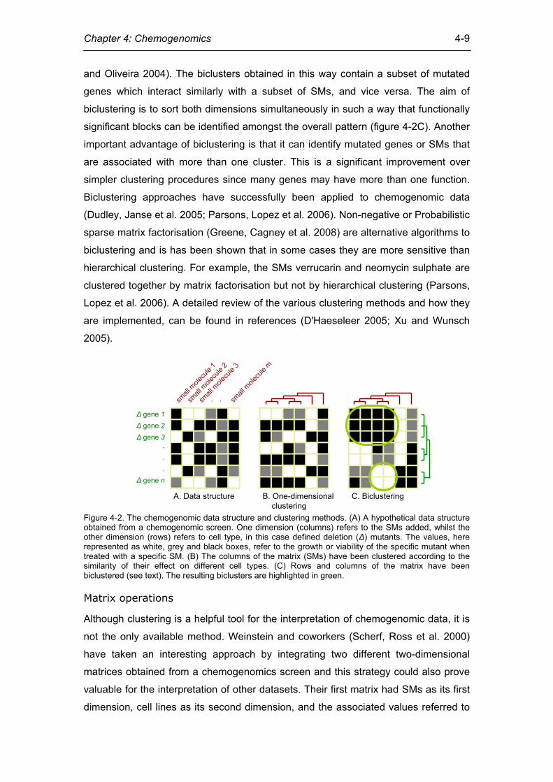
Figure 4-2. The chemogenomic data structure and clustering methods. (A) A hypothetical data structure obtained from a chemogenomic screen. One dimension (columns) refers to the SMs added, whilst the other dimension (rows) refers to cell type, in this case defined deletion (∆) mutants. The values, here represented as white, grey and black boxes, refer to the growth or viability of the specific mutant when treated with a specific SM. (B) The columns of the matrix (SMs) have been clustered according to the similarity of their effect on different cell types. (C) Rows and columns of the matrix have been biclustered (see text). The resulting biclusters are highlighted in green.
Matrix operations
Although clustering is a helpful tool for the interpretation of chemogenomic data, it is
not the only available method. Weinstein and coworkers (Scherf, Ross et al. 2000)
have taken an interesting approach by integrating two different two-dimensional
matrices obtained from a chemogenomics screen and this strategy could also prove
valuable for the interpretation of other datasets. Their first matrix had SMs as its first
dimension, cell lines as its second dimension, and the associated values referred to

Chapter 4: Chemogenomics
4-10
differential growth. In a second matrix, genes were represented in the first dimension,
cell lines in the second dimension, and the associated values referred to transcript
levels as measured by microarrays. The common dimension in both matrices was the
cell lines. The authors then correlated the expression of each gene in each cell line
with its response to each SM and thereby obtained a third two-dimensional matrix,
which has SMs as one dimension and genes as the other dimension. From this
matrix, the authors could identify the genes that are expressed at a differential level
in cell lines that have differential sensitivity to a specific SM. In this way, they could
show how the transcript levels of particular genes relate to sensitivity to specific SMs.
Matrices can in many cases also be visualised and interpreted in networks. SM-gene
networks have also been used to visualise and analyse chemogenomic-like datasets
(Haggarty, Koeller et al. 2003; Sharom, Bellows et al. 2004; Lamb, Crawford et al.
2006; Ma'ayan, Jenkins et al. 2007; Yildirim, Goh et al. 2007) (figure 4-3). One
conclusion that has been possible from the analysis of such drug-target networks is
that there has been a trend for more rational drug design over the last decade
(Yildirim, Goh et al. 2007; Wuster 2008). Later in this chapter I introduce the concept
of chemogenomic networks, which make use of the idea that matrices can be
visualised and interpreted as networks.
small molecule (SM)target protein
target proteinnetwork
SM-targetnetwork
SMnetwork
Figure 4-3. A bipartite network of drugs and their target proteins (drug-target network; centre panel) contains the information to derive both the target protein network and the drug network (Yildirim, Goh et al. 2007). In the target protein network (left panel) two proteins are linked if they are targeted by the same SM. In the drug network (right panel) two drugs are linked if they target the same protein. The giant component of each network is highlighted in light green.
Applications
The immediate purpose of a chemogenomic screen is to characterise the effect a set
of SMs has at the level of genes or proteins. From a biotechnological point of view,
such chemogenomics data can allow for the identification of proteins as novel drug
targets (Bredel and Jacoby 2004). In a screen of SMs against a library of
heterozygous yeast deletions, the gene products that interact with each of the SMs
can be identified. For example, in a chemogenomic screen of mammalian cell lines

Chapter 4: Chemogenomics
4-11
STAT3 could be identified as a potential target for apratoxin A, an SM that is
cytotoxic against tumour cells (Luesch, Chanda et al. 2006). Many yeast genes have
orthologues in humans (Hohmann 2005), which raises the possibility that interactions
with SMs might also be conserved and that orthologues could be potential drug
targets or might aid in gaining an understanding of the side effects of drugs at the
molecular level (Luesch 2006). Nevertheless, it is not clear how well the responses to
SMs are conserved between distantly related organisms. I address this question later
in this chapter. Rapamycin is an example of an SM for which it is known that the
molecular mechanism of action is conserved between S. cerevisiae and humans
(Butcher, Bhullar et al. 2006). This is of particular interest as the majority of drugs are
SMs (Lipinski and Hopkins 2004).
SMs that are found to be active against specific proteins could also serve as
alternatives to genetic methods. In reverse genetics, in order to disrupt the function of
a protein, the DNA sequence that encodes the protein is mutated. Although this
approach has generated a large variety of useful data, it has some drawbacks. First
of all, mutagenesis can be difficult to implement in higher animals such as mammals.
Furthermore, mutagenesis strategies do not exhibit a large degree of spatial and
temporal flexibility, since it is difficult to mutate a gene for only a transient period of
time or in a limited and clearly defined set of cells. An additional problem is that in
multifunctional proteins it can be difficult to disrupt only one protein function whilst
leaving others intact. Chemical genetics has the potential to overcome these
problems (Stockwell 2000; Stockwell 2004; Spring 2005; Florian, Hümmer et al.
2007). The ultimate goal of chemical genetics is to identify SMs that are able to
modulate the function of as many proteins in a cell as possible, either by simulating a
gain-of-function or of a loss-of-function mutation. It has been estimated that between
8 and 14 percent of proteins in eukaryotic genomes are 'druggable' in this way
(Hopkins and Groom 2002). Chemical genetics can be more easily employed in
mammalian cells than mutagenesis strategies and in a manner that is specific to a
set of clearly defined cells, or during a clearly defined time window by adding and
removing the compounds used in the screen. Furthermore, in a multifunctional
protein potentially only one specific function could be modulated without affecting the
others.
The potential of chemical genetics for drug development is well recognised. Recent
applications include the targeting of cancer cell lines that carry mutations in cancer
pathways with specific SMs (Dolma, Lessnick et al. 2003; Rognan 2007) or the use

Chapter 4: Chemogenomics
4-12
of SMs to direct differentiation of stem cells (Huangfu, Maehr et al. 2008; Borowiak,
Maehr et al. 2009; Chen, Borowiak et al. 2009). However, other areas of
biotechnology, including green biotechnology might also benefit from chemical
genetics. Crop plants could be improved with the use of SMs that target specific
proteins, for example those involved in drought resistance pathways (Raikhel and
Pirrung 2005). Since such SMs can be applied in a manner similar to pesticides, the
introduction of genetically modified crops that is often associated with environmental,
legal, or technical difficulties, could be avoided.
Besides these practical applications, chemogenomics data can also offer
fundamental biological insights. Grouping genes according to their chemogenomic
profiles can lead to the identification of clusters that are enriched for functional
categories as defined by the Gene Ontology (GO) database (Ashburner, Ball et al.
2000). If a gene of previously unknown function is found in such a cluster, it is likely
that it has a similar function to the other genes in the same cluster. Chemogenomics
could therefore contribute to the determination of the function of genes whose
function was previously unknown (Dudley, Janse et al. 2005). Moreover, it might
even be possible to define novel functional classes of genes. More specifically, if an
SM causes decreased viability when a set of genes is deleted, this set of genes can
be interpreted as being necessary for conferring resistance to the SM. Therefore,
these genes might have a previously unknown function in common. For example,
deletion of members of the protein complexes SAGA, Swi/Snf and Ino80 each
caused sensitivity to cadmium, cycloheximide, hydroxyurea, and glycerol (Dudley,
Janse et al. 2005). Therefore, it has been assumed that these complexes share a
function, which is to regulate genes that are required in the presence of these SMs.
Chemogenomic networks
Understanding and interpreting the data obtained from a chemogenomic screen is
not trivial, as often the observed effects are not direct. However, in most cases it is
true that if a defined mutant is less viable in the presence of an SM than in its
absence, then the gene that has been mutated has some importance for resistance
to the SM.
This makes a novel method for interpreting chemogenomic data possible that
involves the construction of chemogenomic networks (figure 4-4). Nodes in
chemogenomic networks are genes. Two genes are linked by an edge if they have
one or more SMs in common that cause decreased viability when either of the two

Chapter 4: Chemogenomics
4-13
genes is deleted. Because two genes can be deleterious when deleted in the
presence of more than one different SM, edges in a chemogenomic network have a
weight, which is an integer greater or equal to one. For example, if the edge
connecting two genes has a weight of four, this means that there are four different
SMs that cause a decrease in viability if either of the genes is deleted.
Although it is often assumed that drugs that have the highest selectivity for the
protein they bind are the most effective, this may not be the case (Hopkins, Mason et
al. 2006; Hopkins 2008; Nobeli, Favia et al. 2009). Instead, many of the most
effective drugs bind multiple proteins instead of single targets. Chemogenomic
networks may provide a way of rationally identifying clusters of gene products that
are targeted by the same SMs. If such a cluster is implicated in a certain disease,
SMs that target all or most of the genes of the cluster will be strong candidates for
further investigation, although they may not have been identified as being candidates
when only considering one SM-protein interaction at a time.
2 31
A
B
F
E
C D
2 31
F
E
2 31
E
A
B
C D
A
B
C D
F
E
A
B
C D
F
Chemo-genomicnetworkA
BCDEF
smallmolecules
stra
in li
brar
y
1 2 3SMs
strainlibrary
Figure 4-4. As any network, chemogenomic networks consist of nodes and edges that connect the nodes. In chemogenomic networks, the nodes are genes or strains whilst the edges are relationships between these genes. Two genes are connected by an edge if they are sensitive to the same SM (SM). An edge is therefore an SM that causes a decrease in viability if either of the two genes it connects is deleted. Therefore, the edges in a chemogenomic network are weighted and undirected. This figure shows how a chemogenomic network is constructed. Starting with the chemogenomic data structure (panel 1; decreases in viability are symbolised by dark green), each SM is considered in turn. If the SM causes decreased viability in more than two strains, the edge weight between the two strains is increased by one.
Results and discussion
The properties of a chemogenomic network are dependent on the dataset that is
used to generate it. In a chemogenomic dataset that uses twenty different SMs, the
maximum possible weight of an edge is twenty. Furthermore, the network
constructed from such a dataset can be expected to have a lower graph density (the
proportion of all possible edges that is actually observed) than a network constructed
from a dataset which uses one thousand different SMs. For comparing
chemogenomic networks, it is therefore important to keep these issues in mind and
to counteract them, for example by filtering the network by only including edges
above a threshold weight.

Chapter 4: Chemogenomics
4-14
Interpretation of a chemogenomic network
Two genes are linked by an edge in a chemogenomic network if both are needed for
resistance to the same SM (see Materials and Methods). This suggests that the two
genes have complementary functions. Figure 4-5 shows a chemogenomic network
that has been generated using previously published data (Parsons, Lopez et al.
2006). In the figure, clusters of genes with a grey background are highlighted
because they share common functions: ARN1 and ARN2 both are transporters that
are specific to siderophore-iron chelates; RIP1 is cytochrome-c reductase whilst
COX9 is a cytochrome-c oxidase; and DUG2, APE3, and PCA1 all are peptidases or
hydrolases (http://www.yeastgenome.org/; last accessed 20 July 2009). The function
of open reading frame YBR284W is unknown, but due to its association with three
hydrolases in the chemogenomic network it is plausible to assume that it is one as
well. It is also interesting to note that all four genes of this cluster are encoded within
15 open reading frames of each other on chromosome II. This demonstrates that
edges in chemogenomic networks can be used to identify functional similarities
between genes.
PAN3
CTR1
PET130
OCA5
SRN2
LUG1
RIM21
ZAP1
CAF40
YGR122W
YPT6
YBR246W
COX9
YBR284WVPS21
LAS21
BUD25
SWA2
PEP8
DAL5
DUG2
MCH5
YIL077C
YIR016W
YKL023W
SMI1
PIN4
VPS52
CDC73
GOS1
VAM3
LSM1
SOP4
VAM7
ATG15
FTR1
ECM34VAM10
RBK1
TOM5
MIG1
FET3
MLP1
UNG1
RPL12B
SHU1
SUR4
ARN2
YPL105C
PHO86
END3
URE2
WSC4
CHS5
YPT7
COG6YPL158C
PAT1
SPO22
VPS71
SNF8
APL5
SHE4
VPS30
REG1
MDM20
YCR045C
RIP1
PEP7
PCA1
VPS9
ARN1
NUC1
VPS27
YIL092W
MOG1
POR1
APE3
TEF4
YAR029W
WHI3
VPS24
GMH1
APQ12
ADA2
BEM1
SNX3
SKT5
GCN5
YDJ1
RPS8A
Figure 4-5. Chemogenomic network filtered for edges with a weight of 20 or more. That is to say, two genes are only connected if they are important for resistance to the same 20 or more SMs. Only the largest connected component of the network is shown. The clusters of genes with a grey background are highlighted because it is known that they also share common functions.

Chapter 4: Chemogenomics
4-15
Properties of the chemogenomic network
To ascertain the overlap between two networks, such as the chemogenomic network
and the protein-protein interaction network, I first created a list of nodes which appear
in both networks. Next, I went through both networks and retained only those edges
which connected two nodes which were both on the list. The overlap between the two
networks was then measured by counting the number of edges they had in common.
To assess the significance of this result, I generated a null distribution of overlapping
edge counts by permutating the node labels of the graphs. The Z score of the
observed overlapping edge count relative to this distribution is given below (table 4-2).
Table 4-2. Parameters of the chemogenomic network at different minimum edge weights. The edge weight refers to how many SMs both nodes connect by the edge interact with. Whilst it is clear that there is a larger than expected overlap between the chemogenomic network and the protein interaction network, no such effect can be seen for the transcription interaction network, in which two genes are connected if they are regulated by the same transcription factor (target gene co-regulatory network). In many cases a decrease in growth rate or fitness in a certain combination of SM
and heterozygous deletant will not be indicative of a direct and physical interaction
between the SM and the gene whose dosage has been increased. The gene may
instead encode a protein that compensates for the direct effect of the SM (Venancio,
Balaji and Aravind 2009; Mol BioSyst (in print)). The extent to which such “buffer
genes” contribute to the interactions observed in chemogenomic data is not known.
As a widespread occurrence of this compensation effect could severely skew the
interpretation of chemogenomic data, more research in this area is needed.
In the chemogenomic networks described above, genes that respond to the same
SMs are connected. Alternatively, one can envisage a network that has SMs as
nodes. These nodes are connected if they interact with the same gene (figure 4-3). In
such a way, it may be possible to identify clusters of SMs with similar biological
activities. In the next section (Linking the chemical and biological properties of SMs),
min edge weight ≥ 1 ≥ 2 ≥ 5 edge count 2’084’597 817’683 149’374 connected node count 3’189 2’497 1’391 graph density 0.41 0.26 0.16 min degree mean degree max degree
44 1’307.367
2’870
2 654.93
2’169
1 214.77
1’046 min weight mean weight max weight
1 1.916
29
2 3.336
29
5 6.977
29 clustering coefficient 0.67 0.58 0.54 protein interaction edge overlap – absolute – Z score
4’870 5.43
2’579 8.89
819
13.30 transcriptional interaction edge overlap – absolute – Z score
123’155
1.58
47’087
-0.30
7’615 -1.46

Chapter 4: Chemogenomics
4-16
I approach this problem from a different angle by asking if SMs that have similar
chemical properties also have similar biological properties.
Materials and methods
Data acquisition
The chemogenomic data from which the chemogenomic network used in this
analysis was constructed was published by Parsons et al. (Parsons, Lopez et al.
2006). The dataset describes the sensitivity of a haploid S. cerevisiae mutant library
to 82 SMs.
The protein-protein interaction network was obtained from the BioGRID database
(Stark, Breitkreutz et al. 2006), which combines information on protein-protein
interaction from various sources and types of experiments. The transcription
regulatory network was based on ChIP-chip data (Lee, Rinaldi et al. 2002; Harbison,
Gordon et al. 2004; Balaji, Madan Babu et al. 2006), which identifies direct in vivo
DNA binding events for transcription factors. According to this network, 144
transcription factors regulate 4’347 target genes via 12’230 regulatory interactions. In
order to make the transcription regulatory network comparable to the chemogenomic
network, it was processed in such a way that target genes that are regulated by the
same transcription factor are connected by edges. The resulting network is, strictly
speaking, not a transcription regulatory network, but a target gene co-regulatory
network.
Construction of the chemogenomic network
The chemogenomic network is constructed by collapsing a bipartite network with two
types of nodes into a simple network with only one type of node. In the initial bipartite
network, the two types of nodes are SMs and genes or deletion strains. In the
resulting simple network, genes are the only type of node. In this network, two genes
are connected by an edge if they have one or more SMs they interacted with in the
initial network in common. The edge weight corresponds to the number of those
common SMs. The chemogenomic network can be constructed by considering one
SM at a time, and connecting all genes that interact with it to each other (figure 4-4).
This means that the chemogenomic network will be densely connected if SMs tend to
interact with many genes in the initial bipartite graph. Therefore, it can be useful to
filter edges that have a low weight (that is to say, that symbolise interaction of genes
with only a few common SMs).

Chapter 4: Chemogenomics
4-17
Computation of network parameters and overlap with other networks
Network parameters were computed using the statistical language R and the
package igraph (http://cneurocvs.rmki.kfki.hu/igraph/). Overlap with the protein-
protein interaction network and the transcription regulatory network was assessed
using in-house Perl scripts. For this, all nodes that do not appear in both networks to
be compared were deleted. Then, the number of common edges between the
networks was counted. The significance of the overlap between networks was
assessed by randomising the networks by permutating the node labels and repeating
the analysis 1’000 times.
Linking the chemical and biological properties of small
molecules
Not all sections of chemical space are equally likely to contain SMs that have a
certain biological activity. This is the basic assumption of quantitative structure-
activity relationships (QSAR), which describes how chemical structure is associated
with biological activity. The central tenet of QSAR is that similar SMs bind similar
proteins (Klabunde 2007). This insight enables us to define areas of chemical space
that are occupied by SMs with specific affinity for certain protein families.
By focussing on those areas of chemical space that contain SMs with a biological
activity of interest, it is possible to make the process of drug lead identification more
rapid and efficient. By analysing the chemical properties of approved drugs, Lipinski's
rule of five was discovered (Lipinski, Lombardo et al. 2001). This “rule” states that
most drugs that have been approved by the American Food and Drug Administration
(FDA) have less than five hydrogen-bond donors, less than ten hydrogen-bond
acceptors, a log P value (a measure of hydrophobicity) of less than five, and a
molecular weight of less that 1’500 Da. Therefore, SMs with known structures can be
pre-screened in silico prior to a chemogenomic experiment to select those that are
most likely to have certain biological activities.
However, Lipinski’s rule is limited in its usefulness to chemogenomic screens carried
out in yeasts such as S. cerevisiae and Schizosaccharomyces pombe as it has been
developed to describe the druglikeness of approved drugs in humans. It is not clear if
the same limitations to molecular properties also apply to those SMs that show
bioactivity in yeasts. Here, I address this question by first computing the molecular
properties of SMs, including the predicted octanol-water partition coefficient (log P),

Chapter 4: Chemogenomics
4-18
the polar surface area, the number of atoms, the molecular mass and volume, the
number of hydrogen bonds and acceptors, the number of rotable bonds, and the
number of violations of Lipinski’s rule. I then compare those properties between SMs
that are bioactive in S. cerevisiae and those that are not. Furthermore, I ask whether
there are properties that distinguish SMs that are active in S. cerevisiae from those
that are active in Sc. pombe. In the following, I use the term bioactivity to mean the
ability of a compound to inhibit the growth of a yeast colony.
In order to determine whether SMs that are bioactive in S. cerevisiae tend to have
different molecular properties from those SMs that are not bioactive, I analysed two
distinct datasets. The first dataset (dataset A) has until now not been published and
describes the IC50 values of 2’961 SMs in both S. cerevisiae and Sc. pombe. The
second dataset (dataset B) has been created by a high-throughput screen by an NCI
yeast anticancer drug screen and separates 87’264 SMs into those that have an
effect on the growth of S. cerevisiae and those that do not (see Materials and
Methods).
Results and discussion
In order to assess whether any molecular properties are significantly distinct for the
SMs that are bioactive in S. cerevisiae and Sc. pombe compared to those SMs that
are not, I analysed two distinct datasets, A and B (see Materials and Methods).
What differentiates bioactive small molecules from others?
For dataset A, there is a clear difference between active and non-active SMs for a
number of chemical descriptors. The strongest predictor of biological activity is log P,
a measure of hydrophobicity (table 4-3), which was more than 80% larger in active
SMs than in inactive ones (p < 5.54 · 10-12).
Bioactive SMs on average tend to be more hydrophobic, have a lower polar surface
area, have a higher molecular weight, a lower number of hydrogen bond acceptors, a
lower number of hydrogen bond donors, and a higher volume than the other SMs
screened. Furthermore, a bigger proportion of bioactive compounds, compared to
compounds that are not bioactive, violate one or more of Lipinski's rules.

Chapter 4: Chemogenomics
4-19
Property Explanation Mean
active Mean inactive
Wilcoxon test p-value
logP predicted octanol-water partition coefficient log P (hydrophobicity)
3.59 1.98 5.5 · 10-12
PSA topological molecular polar surface area (important to predict drug transport properties)
55.32
80.97 1.7 · 10-9
natoms number of atoms 22.99 22.63 0.10 MW molecular weight 352.32 326.90 1.5 · 10-4 nON number of hydrogen bond acceptors 4.06 5.47 3.1 · 10-8 nOHNH number of hydrogen bond donors 1.15 2.14 6.3 · 10-9 nviolations how many of Lipinski's rules are violated 0.37 0.33 0.08 nrotb number of rotable bonds (measure of molecular
flexibility) 4.54 3.92 0.40
volume molecular volume in Å3 299.00 284.20 4.6 · 10-3 Table 4-3. Active SMs are defined as those that have an IC50 value of less than 100 μM in both species. Inactive SMs are those that have a higher IC50 value in either or both species. The Wilcoxon test p-value indicates how likely it is that the descriptor is the same for SMs that hit S. cerevisiae and Sc. pombe, and SMs that hit neither. These rules state that the majority of approved drugs have less than five hydrogen
bond donors, less than ten hydrogen bond acceptors, a log P value of less than five,
and a molecular weight of less than 500 Da (Lipinski, Lombardo et al. 2001). In all
cases, the majority of SMs that I defined as being bioactive against the two fungi
follow these rules. However, in the case of log P and molecular weight, the bioactive
SMs are closer to Lipinski's threshold values than the drugs that are not bioactive.
In order to confirm the chemical differences between SMs that are bioactive and
those that are not, I performed principal component analysis using the nine
descriptors mentioned above as initial dimensions. After dimensionality reduction, the
difference between the two types of molecules could be confirmed. It has previously
been shown that there are differences between SMs from combinatorial synthesis,
and drugs as well as natural products (Feher and Schmidt 2003). My analysis shows
that there are also significant differences within classes of SMs according to their
bioactivity.
In order to confirm these results, I repeated the analysis using a previously published
dataset that was larger than the one used above. In the initial stage of an anticancer
drug screen, 87’264 SMs were tested against six different strains of S. cerevisiae. Of
these, 12’068 had a strong effect on yeast growth and 75’196 did not. The results of
this screen have been made available online (http://dtp.nci.nih.gov/yacds/index.html;
last accessed 20 July 2009) and constitute dataset B. As before, I determined the
molecular properties of the tested drugs to see which ones are predictive of activity.

Chapter 4: Chemogenomics
4-20
-800 -600 -400 -200 0 200 400
-200
-150
-100
-50
050
100
PCA of molecular properties
PC1
PC
2
Figure 4-6: Plot of the first two principal components (PCs) of the molecular properties of the 2’961 SMs of dataset A. Active SMs (IC50 < 100 μM) are in red, inactive SMs in grey. The first principal component (PC1) explains 92% of the variance in the data, PC2 explains 6%. The same descriptors are over- and underrepresented according to this dataset
compared to the 2’961 SMs in dataset A. Property Explanation Mean
active Mean inactive
Wilcoxon test p-value
logP predicted octanol-water partition coefficient log P (hydrophobicity)
3.41 2.44 < 2.2 · 10-16
PSA polar surface area (important to predict drug transport properties)
61.07 66.16 < 2.2 · 10-16
natoms number of atoms 23.40 20.54 < 2.2 · 10-16 MW molecular weight 351.91 297.96 < 2.2 · 10-16 nON number of hydrogen bond acceptors 4.42 4.70 < 2.2 · 10-16 nOHNH number of hydrogen bond donors 1.22 1.38 < 2.2 · 10-16 nviolations how many of Lipinski's rules are violated 0.39 0.25 < 2.2 · 10-16 nrotb number of rotable bonds (measure of molecular
flexibility) 4.90 4.39 < 2.2 · 10-16
volume molecular volume in Å3 300.91 262.36 < 2.2 · 10-16 Table 4-4. The Wilcoxon test p-value indicates how likely it is that the descriptor is the same for SMs that hit S. cerevisiae and those that do not. This table is similar to table 4-3, but is based on a different dataset (87’264 SMs from an NCI cancer drug screen).
What differentiates small molecules that hit S. cerevisiae from those that
hit Sc. pombe?
Having established that there are chemical properties that allow distinguishing
between SMs that are bioactive and those that are not, it is of interest to establish
whether these properties vary between organisms. I therefore compared the
chemical properties of SMs that are bioactive in S. cerevisiae to the properties of
SMs that are bioactive in Sc. pombe. There are several important differences
between the two species that would explain why such differences in sensitivity to

Chapter 4: Chemogenomics
4-21
certain SMs exist, including differences in the length of cell cycle phases, or the
presence of RNAi machinery in Sc. pombe but not in S. cerevisiae.
5411559
2733
S.cerevisiae
S.pombe
Figure 4-7: Of 2’961 NCI SMs, the majority that has an IC50 value of less than 100 μM in one species also has an IC50 value of less than 100 μM in the other species. This indicates that an SM that is bioactive to one species is also likely to be bioactive in the other species.
IC50 < 1’000 μM IC50 < 100 μM IC50 < 10 μM IC50 < 1 μM hits S. cerevisiae only 84 59 20 2 hits Sc. pombe only 55 115 48 4 hits S. cerevisiae and Sc. pombe 132 54 48 29 hits neither 2’690 2’733 2’845 2’926 p-value < 2.2 · 10-16 < 2.2 · 10-16 < 2.2 · 10-16 1.89 · 10-7
Table 4-5: As figure 4-7, but at multiple different IC50 cut-offs. The strong overlap between SMs that hit Sc. pombe and S. cerevisiae does not depend on the IC50 cut-off used. It could be that some SMs are bioactive in one organism but not the other because
they have different molecular properties. As before, I obtained the molecular
structures of each of the SMs that have different bioactivity in the two species and
computed nine properties for each of them in order to assess whether one of these
properties was significantly distinct for the SMs that hit one organism but not the
other. No significant result could be found, indicating that bioactivity in S. cerevisiae
is a good predictor of bioactivity in Sc. pombe and vice versa. Property Explanation Mean S.
cerevisiae Mean Sc. pombe
Wilcoxon test p-value
logP predicted octanol-water partition coefficient log P (hydrophobicity)
2.83 3.13 0.46
PSA polar surface area (important to predict drug transport properties)
66.01 61.46 0.71
natoms number of atoms 22.75 23.04 0.85 MW molecular weight 334.30 336.76 0.97 nON number of hydrogen bond acceptors 4.52 4.21 0.66 nOHNH number of hydrogen bond donors 1.63 1.74 0.91 nviolations how many of Lipinski's rules are violated 0.27 0.43 0.09 nrotb number of rotable bonds (measure of molecular
flexibility) 3.62 4.28 0.99
volume molecular volume in Å3 288.12 296.88 0.56 Table 4-6. Properties of drugs that only hit S. cerevisiae versus those that only hit Sc. pombe (IC50 < 1’000 μM). The Wilcoxon test p-value indicates how likely it is that the descriptor is the same for drugs that hit S. cerevisiae and drugs that hit Sc. pombe.

Chapter 4: Chemogenomics
4-22
Conclusions
Some of the above observations on the differences between biologically active and
inactive SMs could be due to the way the chemical libraries that were tested were
generated. The removal of chiral centres, introducing additional flexibility into the
molecule and decreasing its size often lead to lower activity (Feher and Schmidt
2003). As chemical libraries are often created doing exactly those things, this may
explain why, for example, the molecular weight is larger for SMs that are active
compared to those that are inactive. Filtering chemical libraries for SMs with
properties that are enriched in the bioactive set could therefore increase the
efficiency of such screens.
Materials and Methods
Two datasets measuring the bioactivity of SMs in yeast were used.
The first dataset (dataset A) was created by Laura Schuresko-Kapitzky of the
University of California, San Francisco and Scott Lokey of the University of California,
Santa Cruz (unpublished). It describes the IC50 values of 2’961 NCI compounds in
both wild-type S. cerevisiae and wild-type Sc. pombe. The data was obtained by
high-throughput yeast halo assays (Gassner, Tamble et al. 2007).
The second dataset (dataset B) describes the bioactivity of 87’264 NCI compounds
on S. cerevisiae strains. In the initial stage of the anticancer drug screen that
produced this dataset, 87’264 drugs were tested against six different strains of S.
cerevisiae. Of these, 12’068 had a strong effect on yeast growth and 75’196 did not
(http://dtp.nci.nih.gov/yacds/index.html).
I downloaded the molecular structures of each of the SMs
(ftp://ftp.ncbi.nih.gov/pubchem/) and computed nine properties for each of them in
order to assess whether one of these properties was significantly distinct for the SMs
that affect growth. SM properties were computed using Molinspiration's mib tool
(http://www.molinspiration.com/). A local version of the mib tool was kindly provided
by John J. Irwin of the University of California, San Francisco.
All data was analysed using a combination of in-house Perl scripts and the statistical
programming language R.

Chapter 4: Chemogenomics
4-23
References
Ashburner, M., C. A. Ball, et al. (2000). "Gene ontology: tool for the unification of biology. The Gene Ontology Consortium." Nat Genet 25(1): 25-9.
Baetz, K., L. McHardy, et al. (2004). "Yeast genome-wide drug-induced haploinsufficiency screen to determine drug mode of action." Proc Natl Acad Sci U S A 101(13): 4525-30.
Balaji, S., M. Madan Babu, et al. (2006). "Comprehensive analysis of combinatorial regulation using the transcriptional regulatory network of yeast." J Mol Biol 360(1): 213-27.
Borowiak, M., R. Maehr, et al. (2009). "Small molecules efficiently direct endodermal differentiation of mouse and human embryonic stem cells." Cell Stem Cell 4(4): 348-58.
Bredel, M. and E. Jacoby (2004). "Chemogenomics: an emerging strategy for rapid target and drug discovery." Nat Rev Genet 5(4): 262-75.
Brenner, C. (2004). "Chemical genomics in yeast." Genome Biol 5(9): 240. Butcher, R. A., B. S. Bhullar, et al. (2006). "Microarray-based method for monitoring
yeast overexpression strains reveals small-molecule targets in TOR pathway." Nat Chem Biol 2(2): 103-9.
Chang, M., M. Bellaoui, et al. (2002). "A genome-wide screen for methyl methanesulfonate-sensitive mutants reveals genes required for S phase progression in the presence of DNA damage." Proc Natl Acad Sci U S A 99(26): 16934-9.
Chen, S., M. Borowiak, et al. (2009). "A small molecule that directs differentiation of human ESCs into the pancreatic lineage." Nat Chem Biol 5(4): 258-65.
Cheng, Y. and G. M. Church (2000). "Biclustering of expression data." Proc Int Conf Intell Syst Mol Biol 8: 93-103.
D'Haeseleer, P. (2005). "How does gene expression clustering work?" Nat Biotechnol 23(12): 1499-501.
Deutschbauer, A. M., D. F. Jaramillo, et al. (2005). "Mechanisms of haploinsufficiency revealed by genome-wide profiling in yeast." Genetics 169(4): 1915-25.
Dolma, S., S. L. Lessnick, et al. (2003). "Identification of genotype-selective antitumor agents using synthetic lethal chemical screening in engineered human tumor cells." Cancer Cell 3(3): 285-96.
Dudley, A. M., D. M. Janse, et al. (2005). "A global view of pleiotropy and phenotypically derived gene function in yeast." Mol Syst Biol 1: 2005 0001.
Ehrlich, P. (1911). "Aus Theorie und Praxis der Chemotherapie." Folia Serologica VII(7): 697-714.
Feher, M. and J. M. Schmidt (2003). "Property distributions: differences between drugs, natural products, and molecules from combinatorial chemistry." J Chem Inf Comput Sci 43(1): 218-27.
Florian, S., S. Hümmer, et al. (2007). "Chemical genetics: reshaping biology through chemistry." HSFP Journal 1(2): 104-114.
Gassner, N. C., C. M. Tamble, et al. (2007). "Accelerating the discovery of biologically active small molecules using a high-throughput yeast halo assay." J Nat Prod 70(3): 383-90.
Gensini, G. F., A. A. Conti, et al. (2007). "The contributions of Paul Ehrlich to infectious disease." J Infect 54(3): 221-4.
Giaever, G., P. Flaherty, et al. (2004). "Chemogenomic profiling: identifying the functional interactions of small molecules in yeast." Proc Natl Acad Sci U S A 101(3): 793-8.
Giaever, G., D. D. Shoemaker, et al. (1999). "Genomic profiling of drug sensitivities via induced haploinsufficiency." Nat Genet 21(3): 278-83.

Chapter 4: Chemogenomics
4-24
Greene, D., G. Cagney, et al. (2008). "Ensemble non-negative matrix factorization methods for clustering protein-protein interactions." Bioinformatics 24(15): 1722-8.
Haggarty, S. J., K. M. Koeller, et al. (2003). "Multidimensional chemical genetic analysis of diversity-oriented synthesis-derived deacetylase inhibitors using cell-based assays." Chem Biol 10(5): 383-96.
Harbison, C. T., D. B. Gordon, et al. (2004). "Transcriptional regulatory code of a eukaryotic genome." Nature 431(7004): 99-104.
Hillenmeyer, M. E., E. Fung, et al. (2008). "The chemical genomic portrait of yeast: uncovering a phenotype for all genes." Science 320(5874): 362-5.
Hohmann, S. (2005). "The Yeast Systems Biology Network: mating communities." Curr Opin Biotechnol 16(3): 356-60.
Hopkins, A. L. (2008). "Network pharmacology: the next paradigm in drug discovery." Nat Chem Biol 4(11): 682-90.
Hopkins, A. L. and C. R. Groom (2002). "The druggable genome." Nat Rev Drug Discov 1(9): 727-30.
Hopkins, A. L., J. S. Mason, et al. (2006). "Can we rationally design promiscuous drugs?" Curr Opin Struct Biol 16(1): 127-36.
Huangfu, D., R. Maehr, et al. (2008). "Induction of pluripotent stem cells by defined factors is greatly improved by small-molecule compounds." Nat Biotechnol 26(7): 795-7.
Klabunde, T. (2007). "Chemogenomic approaches to drug discovery: similar receptors bind similar ligands." Br J Pharmacol 152(1): 5-7.
Lamb, J., E. D. Crawford, et al. (2006). "The Connectivity Map: using gene-expression signatures to connect small molecules, genes, and disease." Science 313(5795): 1929-35.
Lee, T. I., N. J. Rinaldi, et al. (2002). "Transcriptional regulatory networks in Saccharomyces cerevisiae." Science 298(5594): 799-804.
Lipinski, C. and A. Hopkins (2004). "Navigating chemical space for biology and medicine." Nature 432(7019): 855-61.
Lipinski, C. A., F. Lombardo, et al. (2001). "Experimental and computational approaches to estimate solubility and permeability in drug discovery and development settings." Adv Drug Deliv Rev 46(1-3): 3-26.
Lloyd, N. C., H. W. Morgan, et al. (2005). "The composition of Ehrlich's salvarsan: resolution of a century-old debate." Angew Chem Int Ed Engl 44(6): 941-4.
Luesch, H. (2006). "Towards high-throughput characterization of small molecule mechanisms of action." Mol Biosyst 2(12): 609-20.
Luesch, H., S. K. Chanda, et al. (2006). "A functional genomics approach to the mode of action of apratoxin A." Nat Chem Biol 2(3): 158-67.
Luesch, H., T. Y. Wu, et al. (2005). "A genome-wide overexpression screen in yeast for small-molecule target identification." Chem Biol 12(1): 55-63.
Ma'ayan, A., S. L. Jenkins, et al. (2007). "Network analysis of FDA approved drugs and their targets." Mt Sinai J Med 74(1): 27-32.
Madan Babu, M. (2004). Introduction to microarray data analysis. Computational Genomics: Theory and Application. R. P. Grant, Horizon Press (UK): 225-249.
Madeira, S. C. and A. L. Oliveira (2004). "Biclustering algorithms for biological data analysis: a survey." IEEE/ACM Trans Comput Biol Bioinform 1(1): 24-45.
Mnaimneh, S., A. P. Davierwala, et al. (2004). "Exploration of essential gene functions via titratable promoter alleles." Cell 118(1): 31-44.
Muhlrad, D. and R. Parker (1999). "Aberrant mRNAs with extended 3' UTRs are substrates for rapid degradation by mRNA surveillance." Rna 5(10): 1299-307.
Nobeli, I., A. D. Favia, et al. (2009). "Protein promiscuity and its implications for biotechnology." Nat Biotechnol 27(2): 157-67.

Chapter 4: Chemogenomics
4-25
Parsons, A. B., R. L. Brost, et al. (2004). "Integration of chemical-genetic and genetic interaction data links bioactive compounds to cellular target pathways." Nat Biotechnol 22(1): 62-9.
Parsons, A. B., A. Lopez, et al. (2006). "Exploring the mode-of-action of bioactive compounds by chemical-genetic profiling in yeast." Cell 126(3): 611-25.
Perlstein, E. O., E. J. Deeds, et al. (2007). "Quantifying fitness distributions and phenotypic relationships in recombinant yeast populations." Proc Natl Acad Sci U S A 104(25): 10553-8.
Perlstein, E. O., D. M. Ruderfer, et al. (2007). "Genetic basis of individual differences in the response to small-molecule drugs in yeast." Nat Genet 39(4): 496-502.
Raikhel, N. and M. Pirrung (2005). "Adding precision tools to the plant biologists' toolbox with chemical genomics." Plant Physiol 138(2): 563-4.
Rognan, D. (2007). "Chemogenomic approaches to rational drug design." Br J Pharmacol 152(1): 38-52.
Scherf, U., D. T. Ross, et al. (2000). "A gene expression database for the molecular pharmacology of cancer." Nat Genet 24(3): 236-44.
Schuldiner, M., S. R. Collins, et al. (2005). "Exploration of the function and organization of the yeast early secretory pathway through an epistatic miniarray profile." Cell 123(3): 507-19.
Sharom, J. R., D. S. Bellows, et al. (2004). "From large networks to small molecules." Curr Opin Chem Biol 8(1): 81-90.
Spring, D. R. (2005). "Chemical genetics to chemical genomics: small molecules offer big insights." Chem Soc Rev 34(6): 472-82.
Stark, C., B. J. Breitkreutz, et al. (2006). "BioGRID: a general repository for interaction datasets." Nucleic Acids Res 34(Database issue): D535-9.
Stockwell, B. R. (2000). "Frontiers in chemical genetics." Trends Biotechnol 18(11): 449-55.
Stockwell, B. R. (2004). "Exploring biology with small organic molecules." Nature 432(7019): 846-54.
Wuster, A. (2008). "Networking with Drugs." Mol BioSyst 4: 14-17. Xu, R. and D. Wunsch, 2nd (2005). "Survey of clustering algorithms." IEEE Trans
Neural Netw 16(3): 645-78. Yildirim, M. A., K. I. Goh, et al. (2007). "Drug-target network." Nat Biotechnol 25(10):
1119-1126.