GL-TR-89-0319ENVIRONMENTAL RESEARCH PAPERS, NO, 1047

Comparison of Steady State Evaporation Models for ToxicChemical Spills: Development of a New Evaporation Model

TERI L.VOSSLER

Lf

29 November 1989

Approved for public release; distribution unlimited.

ATMOSPHERIC SCIENCES DIVISION PROJECT 6670

GEOPHYSICS LABORATORYHANSCOM AFB, MA 01731-5000

SI

This report has been reviewed by the EBD Public Affairs Office (PA) and isreleasable to the National Technical information Service (NITS).

"This technical report has been reviewed and is approved for publication"

F'OR TH~E COI9IAHD

Atmospheric Structure Branch 'Atmosp•eric Sciences Division

Qualified requesters my obtain additional copies from the Defense TechnicalInformation Center. All others should apply to the National TechnicalInformation Service.

If your address has changed, or if you wish to be removed from the mailinglist, or if the addressee is no longer employed by yur organization, pleasenotify OL/DAA, and GL/LYA Hanscom AFB, M• 01731-5000. This will assist us inmaintaining a current mailing list.

Do not return copies of this report unleas nontractual obligation or noticeson a specific document requires that it be rceturned.

REPO T D CUM NTATON AGEForm ApprovedREPORT~~~ DOUENAIONAG#M No. 0?04-0188

Davis HI~way. Wisl 104, Ade4te, VA 11216.43ft, srd Is Owe &be of Mattagemateod W dget Pepeweek ftedon Pr*et(7045) W- -I'M!-D 3050801. AGENCY US4 ONLY MLaws Werta 8.UPNTAT! 3. R1PO~ TYPE AND DAMu 00"YURU

29NOV 89 Scientific Interim MAY 89 - NOV 894 TITI AN 0U~rL1 .FUNDING NUMINN

Comparison of Steady State Evaporation Models for Toxic Chemical PE - 62101FSpills: Development of a New Evaporation Model PR - 6670

TA- 14

7. PERFORMING ORGANIMTOR NAME(6j XND ADDRENWO) .PRIRP0OMNG ORGOANIZATION

Geophysics Laboratory/LYA IMOL-TR*89-031I anscom, AFB E~-R-89No.3104Massachusetts 017314000RN.14

S. 6PONSORINOJONITORING AGINOY NAME(S) AND ADDIIIIIII(U) 10. MPNSOONNCOMNITORINGIAGICY RIPOWTNUMM

I1i. SUPPLEMENTARY NOTESAir Force Geophysics Scholar*

tie I8TI& BTpieu-nAvEAniurLIy STATIMENT T t~. DOISISTION 0O03APPROVED FOR PUBLIC RELEASE; DISTRIBUTION UNLIMITED jThe United States Air Force handles and stores a number of toxic and hazardous chemicals,Associated with this activity is the threat of accidental release, To determine the downwind threatof a spilled liquid chemical, one must estimate the evaporation rate of the spinled chemical. Asteady state evaporation model is one that calculates the temperature of the spilled chemical poolbased on the net energy input into the pool from all possible sources. The pool temperature is usedto calculate the evaporation rate. Three steady state evaporation modelst are compared, and themost appropriate calculation for each energy input into the pool is identified. A new steady stateevaporation model is presented based on the comparisons. Sensitivity studies are presented insupport of the new model,

f? )~

14. GSUIJOT TIRMO IS. NUMBER OF PONEvaporation, toxidc chemical,- Spills, liquid chemical 56

il PRIC 0331

17T. gQ3J CLOGLMCIATION 11S. IXWASUP1OATION I t.8110AS8IPIOAIION 0. LIMITATION OF AISTWAT

I.UNCLASSIFIED UNCLASSIFIED UNCLASSIFIED BARN6NHS0401 250. #W000r fom 06 (mwy, I9-0

Preosabed by ANS isDOM55101

Preface

The author gratefull acknowledges the assistance of Mr. Bruce Kunkel, who provided acareful and thoughtful review of this report and made many useful suggestions. This reportwas written while the author was an Air Force Oeophysics Scholar, under a programadministered by the Southeastern Center for Electrical Engineering Education.

Aoes~sion For

DTIC TARUwnnounowidJuutifcaiuon tNI'

Di',st z biib t tonl/ _

AvntI.:iI.Llty CodesiP-'I L ind/or

AI

ill

Contents

1. INTRODUCTION 1

2. GENERAL DESCRIPTION OF STEADY STATE ENERGY BALANCE 3

2.1 Heat Due to Solar Radiation (Q.01) 3

2.1.1 SOLAR ALTITUDE ANGLE - COMPARISIONS 32.1.2 SOLAR ALTITUDE ANGLE - RECOMMENDATION 42.1.3 HEAT FROM NET SOLAR RADIATION - COMPARISONS 52.1.4 HEAT FROM NET SOLAR RADIATION - RECOMMENDATION a

2.2 Long Wave Radiation Emitted by the Atmosphere (Q0tm) 7

2.2.1 COMPARISIONS 72,2,2 RECOMMENDATION 7

2,3 Long Wave Radiation Emitted by the Pool (Qpol) 8

2.3.1 COMPARISONS 82.3.2 RECOMMENDATION 8

2.4 Heat Conducted from the Ground (Qgi) 82.4.1 COMPARISONS 82.4.2 RECOMMENDATION 11

2.5 Heat Loss Due to Evaporation (Q.v) 13

2.5.1 COMPARISONS - GENERAL 132.,5.2 MASS TRANSFER COEFFICIENT 142.5,3 MASS DIFFUSMIY 15

V

2.5.4 RECOMMENDATIONS 17

2.6 Sensible Heat Transfer Due to Conduction and Turbulence (Qhs) i82.6.1 COMPARISONS 182.6.2 RECOMMENDATION 19

2.7 Evaporation Rate 20

2.8 Calculation of Liquid Chemical Pool Temperature 21

3. SUMMARY OF THE NEW EVAPORATION MODEL 21

3.1 Heat Due to Net Solar Radiation 23

3.2 Long Wave Radiation Emitted by the Atmosphere and the Pool 24

3.3 Heat Conducted from the Ground 24

3.4 Heat Loss Due to Evaporation 26

3.5 Sensible Heat Transfer Due to Conduction and Turbulence 27

3.6 Pool Temperature Calculation 28

3.7 Chemical Data Base 29

4. NEW MODEL SENSITIVITY STUDIES 80

4.1 Solar Altitude Angle 314.2 Net Heat from Solar Radiation 81

4.3 Long Wavelength Radiation Emitted by the Atmosphere 334.4 Long Wavelength Radiation Emitted by the Pool 34

4.5 Heat Conducted from the Ground 35

4.6 Heat Loss Due to Evaporation 36

4,6.1 PROPERTIES OF VAPOR ABOVE POOL s34.6.2 MASS TRANSFER COEFFICIENT 40

5. CONCLUSIONS 43

REFERENCES 47

vi

Tables

1. Solar Altitude Angle from the Kawamura and MacKay (KM) Model 4and the ADAM Model.

2. Thermal Properties of Different Ground 'Types, 12

3, Input Data Required for Each Model. 22

4. Chemicals in New Evaporation Model Data Base. 295. Default Values of Parameters for Sensitivity Studies. so6. Effect of Solar Altitude Angle on Evaporation Rate. 31

7. Comparison of Methods for Calculating Net Heat from Solar Radiation, 32

8. Calculations for Ille and Springer Atmosphere Emissivity (0,75) ve Kawamura 33and MacKay Atmosphere Emissivity (0.81),

9. Calculations for Ille and Springer Pool Emisstvlty (0.95) vs Kawamura and 34MacKay Pool Emissivity (0,97).

10. Effect of Ground Type on Evaporation Rate. 35

11. ADAM Ground Heat Transfer Coefficient (ADAM hgrd) vs Kawamura and 36MacKay Ground Heat Transfer Coefficient (KM hird},

12. Thermal Conductivity of the Ground: Ground and Liquid Thermal 37Resistance ve Ground Thermal Resistance Only,

13. Evaporation Rates Calculated for Chemical/Air Mixture vs Air Only 38vs Pure Chemical Only.

14, Sensitivity of Pure Chemical Mole Fraction (MF) Calculation. 39

15. Sensitivity of Stability Parameter n, 40

vii

16. Effect of Mass Transfer Coefficient Calculation on Calculated Evaporation Rate, 41

17. Effect of Terrain Type on Calculated Evaporation Rate, 42

18. Effect of Wind Speed on Calculated Evaporation Rate. 42

19. Comparison of Kawamura and MacKay Model with New Model. 43

20. Comparison of ADAM Evaporation Model with New Model. 44

21, Comparison of Modified ille and Springer Model with New Model. 45

viii

Comparison of Steady State Evaporation Modelsfor Toxic Chemical Spills: Development of a

New Evaporation Model

1. INTRODUCTION

The United States Air Force handles and stores a number of toxic and hazardous

chemicals, Associated with this activity is the threat of accidental release of these dangerouschemicals. That threat applies not only to the immediate area of the spill, but to locationsdownwind of the spill. To determine that downwind threat, one must estimate the sourcestrength (evaporation rate) of the spilled chemical. One spill scenario for which one must beprepared is that of a liquid chemical spilled onto the ground so that it forms a pool. Toestimate the evaporation rate from the pool, data including meteorological information,properties of the spilled chemical, characteristics of the spill site, and the size of the spill,must be readily available, The procedure for estimating source strength should be simpleenough to run on a microcomputer with a minimum of knowledge of the program by the user.

Several evaporation models were compared by Kunkel. I The file and Springer 2 model wasIdentified as being the most realistic of the available evaporation models because it allows for

(Received for Publication 28 November 1989)I Kunkel, B.A. (1983) A Comparison of Evaporative Source Strength Models for TbxicChemical Spills, AFOL-TR-83-0307, ADA 139431.

2 Ille, 0. and Springer, C. (1978) The Evaporation and Dispersion of Hydrazine Propellantsfr'om Ground Spills, CEEDO-TR-78-30, ADA 059407.

1

changes in the pool temperature due to evaporation and solar insolation. Kunkel modified theIlle and Springer model so that it includes a parameter, n, which describes the wind velocityprofile. This parameter was referred to by Kunkel as the stability index, It Is a function of

atmospheric stability and surface roughness. It has a significant impact on the calculatedsource strength. A 100 percent change in the stability index number generally results in atleast a 43 percent change in the calculated evaporation rate. 1.2 None of the other modelsdescribed in the comparison by Kunkel considered the wind velocity profile. The Ille andSpringer model with this change will be referred to as the modified Ille and Springer model,

Since the evaporation model comparison by Kunkel, several other evaporation modelshave become available which follow the same general calculation procedure as the Ille andSpringer model. This procedure is a steady state balance of all sources of energy that add to orsubtract from the energy of a pool of liquid which has spilled onto the ground, Each of thesemodels takes a different approach to the calculation of each energy input. This report willserve two purposes: (1) It will compare each of three energy balance evaporation models andidentify the most appropriate calculation for each energy input, and (2) it will present a newenergy balance evaporation model that uses the most appropriate calculations based on thecomparisons.

The models described in this report are (1) the modified Ille and Springer evaporationmodel,1.2 (2) the ADAM model liquid pool evaporation source calculation,3 (3) the Kawamuraand MacKay evaporation model, 4 and (4) the "New" evaporation model. The latter is a newmodel that will be recommended based on examination and evaluation of the other models,

The four models were programmed in the Basic language for the Zenith-248microcomputer. The ADAM model is a large and complex model including many types ofsource strength calculations. A liquid pool evaporation model based on a steady state energybalance is included among those source calculations. The ADAM code for evaporation of apool of liquid was extracted from the ADAM Fortran code and translated into Basic tofunction as a stand-alone model. The Kawamura and MacKay model was taken from itsJournal article description 4 and translated into a Basic code, The modified Ille and Springermodel had already been written in Basic code for the Z-248.

In Section 2, the calculation of each energy term from the modified Ille and Springer,Kawamura and MacKay, and ADAM models are evaluated, Recommendations are made for themost appropriate calculations for a new evaporation model based on evaluations, In Section3, the new model is summarized, In Section 4, sensitivity studies are presented in support ofthe new model, Concluding remarks are made in Section 5.

"3 Raj, P.K. and Morris, JA, (1987) Source Characterization and Heavy Gas Dispersion Modelsfor Reactive Chemicals, AFGL-TR-88-0003 (I), ADA 200121.4 Kawanura, P.,I and MacKay, D. (1987) The evaporation of volatile liquids, Journal qfHazardous Materials, 15:343-364.

2

2. GENERAL DESCRIPTION OF STEADY STATE ENERGY BALANCE

The evaporation rate of a chemical from a pool surface is ultimately a function of poolsurface temperature. The equilibrium surface temperature depends on many avenues of heattransfer to and from the pool. These include solar radiation (Q5oi). long wave radiationemitted by the pool (Qpo1) and the atmosphere (Qatm), convective heat transfer from theatmosphere (Oh-). heat conducted from the ground (Qgrd), and heat loss due to evaporation ,The steady state temperature is the temperature at which the sum of all sources of heat (energy)transported into the pool exactly balances the heat transfer out of the pool; that is, the sum ofenergy terms described above is zero. The steady state energy balance is expressed as:

94O! 01 + aft + poI + Ohe + Gov + Or• W d total'

where Ototal w 0 at steady state. Many of these energy terms can be expressed as a function ofthe pool surface temperature. The equation is solved Iteratively for the pool temperature,which is then used to calculate evaporation rate. The evaporation rate is proportional to themass transfer coefficient at the liquid pool - atmosphere interface and the vapor pressure ofthe chemical, both of which are functions of the pool surface temperature.

2.1 Heat Due to Solar Radiation (,,ol)

The net solar radiation reaching the spilled liquid depends on the amount of cloud cover,the time of day, and the geographical location of the pool, The last two parameters are used tocalculate the solar altitude angle.

2.1.1 SOLAR ALTITUDE ANGLE - COMPARISONS

In the modified Ille and Springer model, the solar altitude angle is input by the user. Thisamounts to a visual estimate of the angle of the sun relative to the surface of the pool. Duringcloudy periods this could be difficult to do,

The ADAM model and the Kawamura and MacKay model calculate the solar altitude angleby similar methods. They both start with the following equation for the solar altitude angle,SA:

sin SA w sin LA sin D + cos LA cos D cos SHA, (2)

3

where LA Is the latitude, D is the solar declination, and SHA is the solar hour angle,The models differ in their calculation of the solar declination and solar hour angle. The

ADAM model follows the procedure of Woolf,5 which computes the exact time of meridian

passage (true solar noon), needed to calculate the solar hour angle, The Kawamura andMacKay model uses the calculations given in Lunde,6 which sets noon equal to 12, The solardeclination calculated by the Kawamura and MacKay model is likewise a simplified version ofthe ADAM model solar declination.

2.1.2 SOLAR ALTITUDE ANGLE - RECOMMENDATION

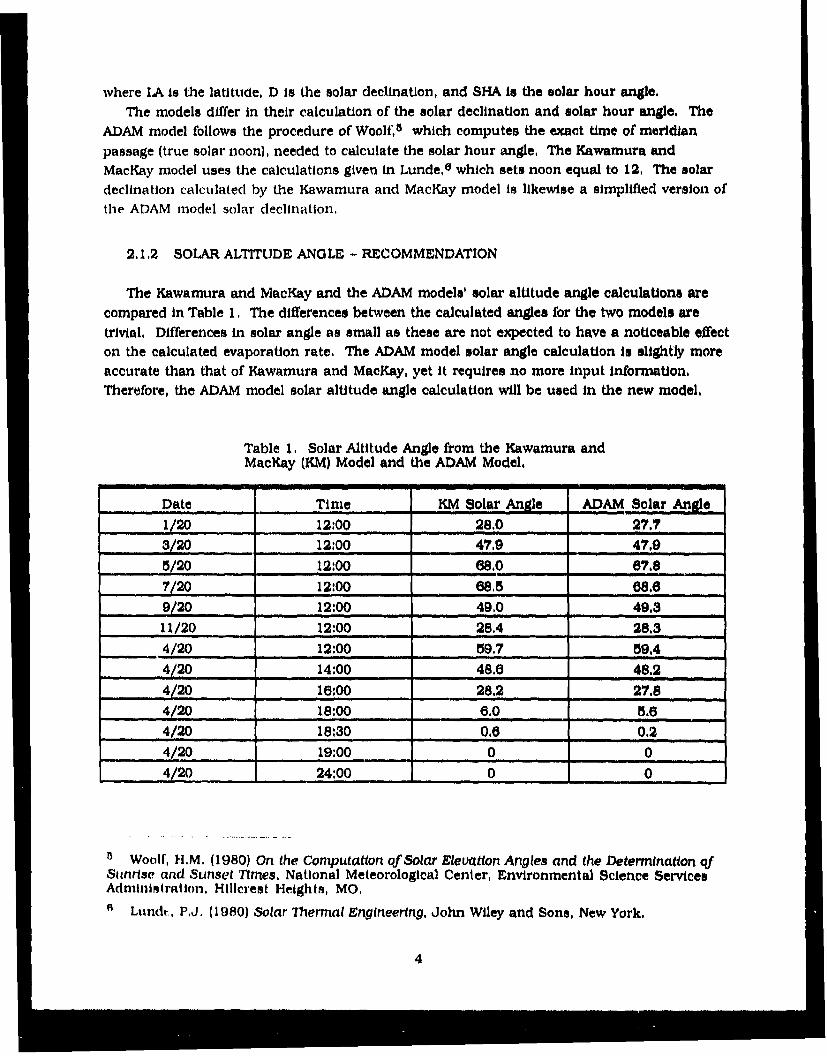
The Kawamura and MacKay and the ADAM models' solar altitude angle calculations arecompared in Table 1, The differences between the calculated angles for the two models aretrivial, Differences in solar angle as small as these are not expected to have a noticeable effecton the calculated evaporation rate. The ADAM model solar angle calculation is slightly moreaccurate than that of Kawamura and MacKay, yet it requires no more input information,Therefore, the ADAM model solar altitude angle calculation will be used In the new model,

Table 1. Solar Altitude Angle from the Kawamura andMacKay (KM) Model and the ADAM Model,

Date Time KM Solar Angle ADAM Solar Angle1/20 12:00 28,0 27.73/20 12:00 47.9 47,95/20 12:00 68.0 67,87/20 12:00 68,5 68.69/20 12:00 49.0 49,311/20 12:00 28.4 28.34-20 12:00 59,7 59,.44/20 14:00 48,, 48.24/20 16:00 28,2 27.84/20 18:00 6.0 5.64/20 18:30 0.6 0.24/20 19:00 0 o .... 0 .......4/20 24:00 0 .. 0 .... .

SWoolf, H.M, (1980) On the Computation of Solar Elevation Angles and the Determination oQJSunrrise and Sunset Times, National Meteorological Center, Environmental Science ServicesAdministration, Hillcrest Heights, MO.

I Lundi, P.J. (1980) Solar Theral Engineering, John Wiley and Sons, New York.

4

2.1,3 HEAT FROM NET SOLAR RADIATION - COMPARISONS

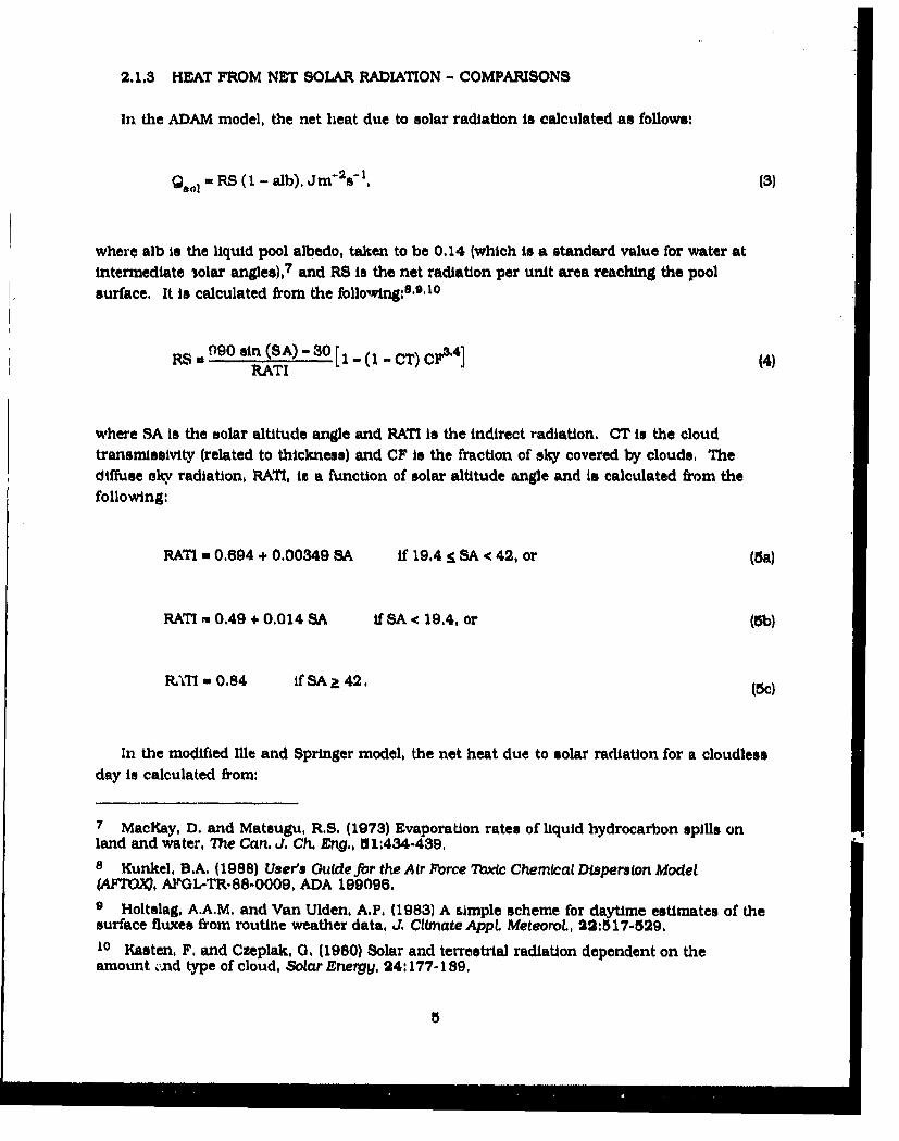
In the ADAM model, the net heat due to solar radiation is calculated as follows:

Q80 1 " RS ( - alb), Jm' 2s8-, (3)

where aib is the liquid pool albedo, taken to be 0.14 (which is a standard value for water atintermediate iolar angles),7 and RS is the net radiation per unit area reaching the poolsurface, It is calculated from the followng:s,, 10

R9 a 9 9 0 sin (SA)- 30 [ 1-(-CT) Ce'4] (4)RATI

where SA Is the solar altitude angle and RATI is the indirect radiation. CT is the cloudtransmissivity (related to thickness) and CF is the fraction of sky covered by clouds, Thediffuse sky radiation, RATI, is a function of solar altitude angle and is calculated from thefollowing:

RATI . 0.694 + 0.00349 SA if 19.4 1 SA < 42, or (Sa)

RATI m 0.49 + 0,014 SA if SA < 19,4, or (Sb)

RAITI = 0.84 if SA _ 42. (5c)

In the modified Ille and Springer model, the net heat due to solar radiation for a cloudlessday is calculated from:

7 MacKay, D. and Matsugu, RS. (1973) Evaporation rates of liquid hydrocarbon spills onland and water, The Can. J. Ch. Eng,, 51:434-439,

8 Kunkel, B.A. (1988) User's Guide for the Air Fbrce Toxic Chemical Dispersion Model(AF4TO., AFGL-TR-88-0009, ADA 199096.

9 Holtslag, A.A.M. and Van Ulden, A.P. (1983) A sImple scheme for daytime estimates of thesurface fluxes from routine weather data, J, Climate AppL MeteoroL, 22:517-529.10 Kasten, F. and Czeplak, 0. (1980) Solar and terrestrial radiation dependent on theamount iý.nd type of cloud, Solar Energy, 24:177-189.

S

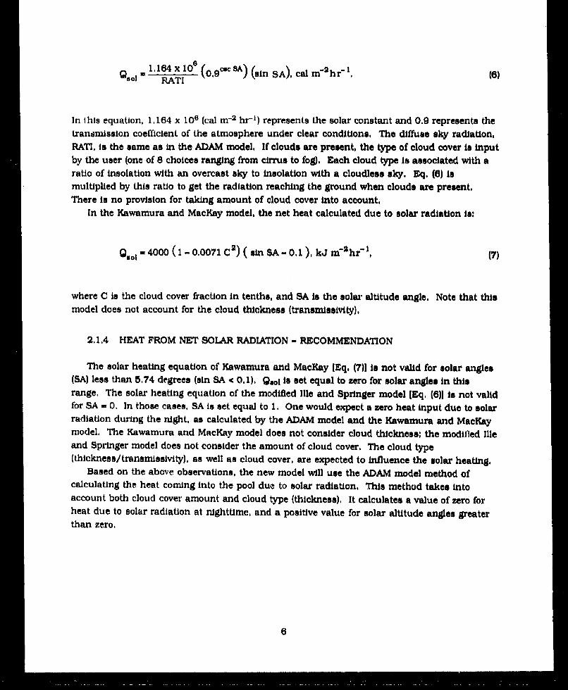
981W1. 164 x10 6 (0 19 cc U) (sin SA), Cal mr2 hr1 . (6)Qsl" RATI

In this equation, 1, 164 x 106 (cal M- 2 hr-1 ) represents the solar constant and 0.9 represents thetransmission coefficient of the atmosphere under clear conditions, The diffuse sky radiation,RATI, is the same as in the ADAM model. If clouds are present, the type of cloud cover is inputby the user (one of 8 choices ranging from cirrus to fog). Each cloud type is associated with aratio of insolation with an overcast sky to insolation with a cloudless sky. Eq. (6) ismultiplied by this ratio to get the radiation reaching the ground when clouds are present.There is no provision for taking amount of cloud cover into account.

In the Kawamura and MacKay model, the net heat calculated due to solar radiation is:

Q.980 4000 (1 - 0.0071 C') ( sin SA - 0.1 ), kJW m 2 hr-', (7)

where C is the cloud cover fraction in tenths, and SA is the solar altitude angle. Note that thismodel does not account for the cloud thickness (transmissivity),

2.1.4 HEAT FROM NET SOLAR RADIATION - RECOMMENDATION

The solar heating equation of Kawamura and MacKay (Eq. (7)1 is not valid for solar angles(SA) less than 5,74 degrees (sin SA < 0.1), 1.Q 0 is set equal to zero for solar angles in thisrange, The solar heating equation of the modified Ille and Springer model [Eq, (6)] is not validfor SA = 0. In those cases, SA is set equal to 1. One would expect a zero heat input due to solarradiation during the night, as calculated by the ADAM model and the Kawamura and MacKaymodel. The Kawamura and MacKay model does not consider cloud thickness; the modifled Illeand Springer model does not consider the amount of cloud cover. The cloud type(thlckness/transmissivity), as well as cloud cover, are expected to influence the solar heating.

Based on the above observations, the new model will use the ADAM model method ofcalculating the heat coming into the pool due to solar radiation. This method takes intoaccount both cloud cover amount and cloud type (thickness), It calculates a value of zero forheat due to solar radiation at nighttime, and a positive value for solar altitude angles greaterthan zero,

6

2,2 Long Wave Radiation Emitted by the Atmosphere (Qatm)

2.2.1 COMPARISONS

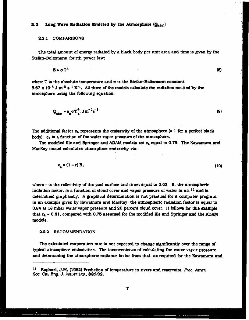
The total amount of energy radiated by a black body per unit area and time is given by theStefan-Boltzmann fourth power law:

E oT 4 (8)

where T is the absolute temperature and a is the Stefan-Soltzmann constant,5,67 x 10-8 J m-2 s-I KX-. All three of the models calculate the radiation emitted by theatmosphere using the following equation:

wer T 4oT, JmIn-2s7"I, (9)

The additional factor ea represents the emissivity of the atmosphere (a I for a perfect blackbody). ea is a function of the water vapor pressure of the atmosphere.

The modified Ille and Springer and ADAM models set ea equal to 0.75. The Kawamnura andMacKay model calculates atmosphere emissivity via:

e (I - r) B, (10)

where r is the reflectivity of the pool surface and is set equal to 0.03. B, the atmosphericradiation factor, is a function of cloud cover and vapor pressure of water in air, 1 1 and isdetermined graphically. A graphical determination is not practical for a computer program.In an example given by Kawamura and MacKay, the atmospheric radiation factor is equal to0.84 at 18 mbar water vapor pressure and 20 percent cloud cover. It follows for this examplethat ea a 0.81, compared with 0.75 assumed for the modified Ille and Springer and the ADAMmodels.

2.2.2 RECOMMENDATION

The calculated evaporation rate is not expected to change significantly over the range oftypical atmosphere emlssivitles. The inconvenience of calculating the water vapor pressureand determining the atmospheric radiance factor from that, as required for the Kawamura and

11 Raphael, J.M. (1962) Prediction of temperature in rivers and reservoirs, Proc. Amer.Soc. Clv. Eng. J. Power Div., 88:P02.

7

MacKay model, is not worth the miginal benefit, Therefore, it is reasonable to assign a

constant value of 0.75 to the atmosphere emissivity, a* in the ADAM and the modified Me and

Springer models.

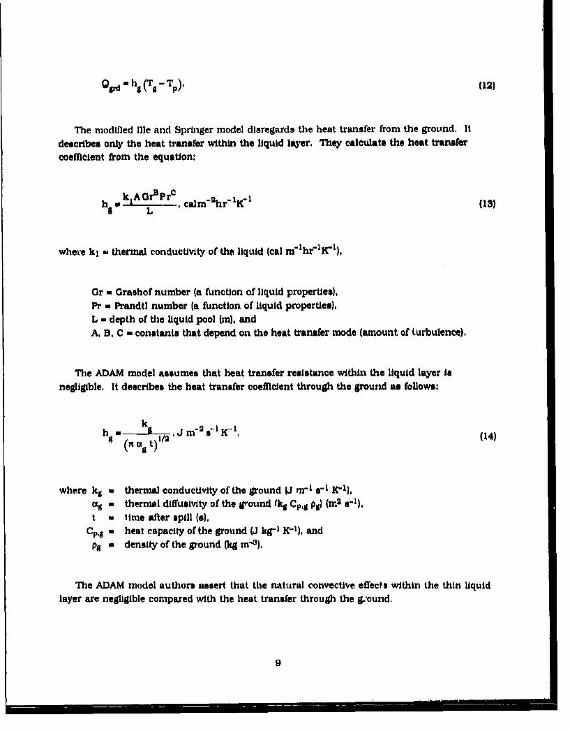
2.3 Long Wave Radiation Emitted by the Pool (Qpel)

2,3,1 COMPARISONS

All three of the models calculate the radiation from the pool from the Stefan-Boltumann

Law:

4GpOt epoT' (IP

The emissivity of the pool (ep) is set equal to 0,95 in the modified Ille and Springer and the

ADAM models, and 0.97 in the Kawamura and MacKay model. These values are approximatelythe emissivity of water. 12

2,3.2 RECOMMENDATION

According to McAdams, 12 the emissivity of water for long wave radiation ranges from 0.95to 0,963 (for temperatures ranging from 0 to 100 degrees Centigrade). For the new model, apool of liquid with emissive properties similar to water near the freezing point will beassumed. This corresponds to an ermssivity of 0.95.

2.4 Heat Conducted from the Ground (0grd)

2,4,1 COMPARISONS

Heat is transferred from the ground to the liquid at the ground surface when the ground iswarmer than the liquid. This heat transfer will decrease with time as the ground temperatureapproaches that of the liquid pool temperature. There will also be thermal resistance withinthe pool of liquid in transferring heat from the bottom of the liquid layer to the top, whereevaporation occurs. Heat transfer from the ground to the liquid is driven by the difference in

temperature between the ground and the pool:

12 McAdams, W.H. (1954) Heat Transmission, 3rd edn., McGraw-Hill Book Company, Inc,,New York.

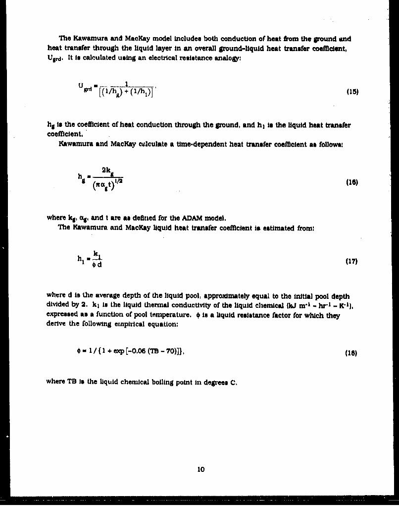
Q u hg(T-T ) (12)

The modified Ille and Springer model disregards the heat transfer from the ground. It

describes only the heat transfer within the liquid layer. They calculate the heat transfer

coefficient from the equation:

h cPrcalmhr" K" (13)a L

where kj so thermal conductivity of the liquid (cal mf'hrWK1 ),

Or = Orashof number (a function of liquid properties),

Pr - Prandtl number (a function of liquid properties),L - depth of the i/quid pool (m), andA, B, C - constants that depend on the heat transfer mode (amount of turbulence),

The ADAM model assumes that heat transfer resistance within the liquid layer isnegligible, It describes the heat transfer coefficient through the ground as follows:

h 9 ( /2 m 2 s7K", (14)

where kg - thermal conductivity of the ground ( rr"1 s" K-'),MIg 0 thermal diffusivity of the ground (kg Cp.V pg) (rn2 s'-1),t • time after spill (a),

Cpg w heat capacity of the ground (J krl K-7), and

Pg = density of the ground (kg re3).

The ADAM model authors assert that the natural convective effects within the thin liquidlayer are negligible compared with the heat transfer through the g.'ound.

9

n s mI . . ... . . .. ...

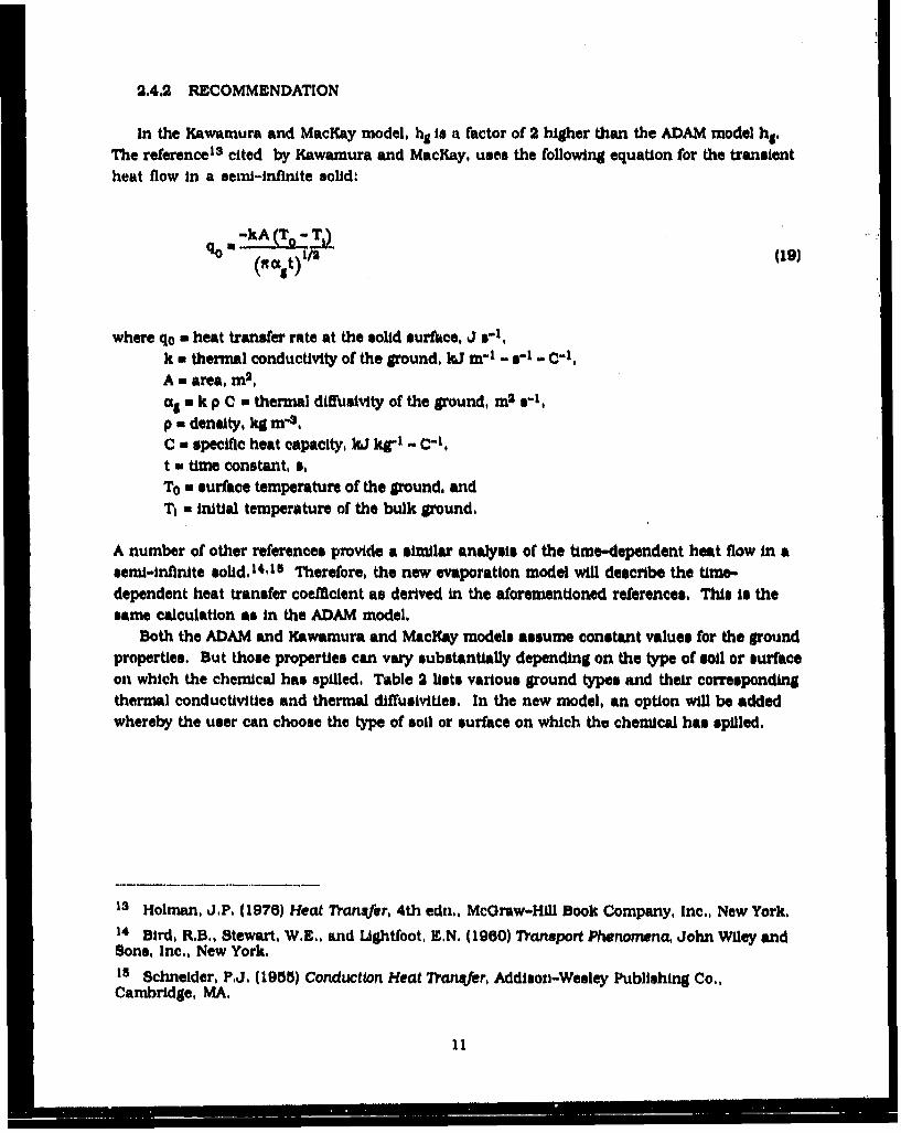
The Kawamura and MacKay model includes both conduction of heat from the ground andheat transfer through the liquid layer in an overall ground-liquid heat transfer coefficlent,Uprd. It Is calculated using an electrical resistance analogy:

(I/h) + (15

hI ts the coefficient of heat conduction through the ground, and h, is the liquid heat transfercoefficient.

Kawamura and MacKay ciculate a time-dependent heat transfer coefficient as follows:

2k

(it a= t)

where kg, a nd t are as defined for the ADAM model,The Kawamura and MacKay liquid heat transfer coefficient is estimated from:

h (17)

where d is the average depth of the liquid pool, approximately equal to the initial pool depthdivided by 2. k1 Is the liquid thermal conducUvity of the liquid chemical (kJ m"! - hr-' - K71),expressed as a function of pool temperature, # is a liquid resistance factor for which theyderive the following einpizlcal equation:

S- I / (fI + exp [-0.06 (TB - 70)]), (18)

where TB Is the liquid chemical boiling point in degrees C.

10

2.4,2 RECOMMENDATION

In the Kawamura and MacKay model, hg is a factor of 2 higher than the ADAM model hg.The reference13 cited by Kawamura and MacKay, uses the following equation for the transientheat flow in a semi-infinite solid:

qoa-kA (TO 1- T9)O t)(19)

where qo m heat transfer rate at the solid surfkce, J s=,k w thermal conductivity of the ground, WJ m-1 - 51- C-1,A = area, m 2,

*s m k p C a thermal diffusivity of the ground, m2 2i,p * density, kg M-3,.C * specific heat capacity, kJ kg- - C-1,t • time constant, s,To m surface temperature of the ground, and

Ta w initial temperature of the bulk ground.

A number of other references provide a sim.ilar analysis of the time-dependent heat flow in asemn-infinite solid. 14,15 Therefore, the new evaporation model will describe the time-dependent heat transfer coefficient as derived in the aforementioned references, This is thesame calculation as in the ADAM model.

Both the ADAM and Kawamura and MacKay models assume constant values for the groundproperties. But those properties can vary substantially depending on the type of soil or surfaceon which the chemical has spilled. Table 2 lists various ground types and their correspondingthermal conductivities and thermal diffuslvities. In the new model, an option will be addedwhereby the user can choose the type of soil or surface on which the chemical has spilled.

13 Holman, J,P, (1976) Heat Transfer, 4th edn., McGraw-Hill Book Company, Inc., New York,

14 Bird, R.,,, Stewart, W.E,, and LIghtloot, EN. (1960) Transport Phenomena, John Wiley andSons, Inc., New York.

15 Schneider, PJ. (1955) Conduction Heat Transfer, Addison-Wesley Publishing Co.,Cambridge, MA.

11

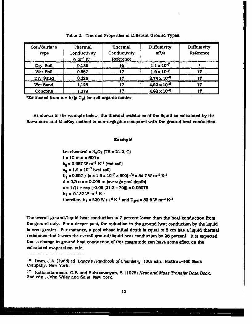
Table 2. Thermal Properties of Different Ground Types.

Soil/Surfare Thermal Thermal Diffusivity DiffusivityType Conductivity Conductivity m2/s Reference

W ar, K-1 Reference

Dry Soil 0,138 16 1.1 x 10.7Wet Soil 0.657 17 1.9 x 10-7 17Dry Sand 0.326 17 2.74 x 10-0 17Wet Sand 1.128 17 4,92 x 10-6 17Concrete 1.279 17 4.92 x 104 17

*Estimated from a a k/(p Cp) for soil organic matter.

As shown in the example below, the thermal resistance of the liquid as calculated by theKawamura and MacKay method is non-negligible compared with the ground heat conduction,

Example

Let chemical = N20 4 (TB a 21.2, C)t a 10 min w 600 sk 0.657 W m- Kr1 (wet soil)

a 1,9 x I0"7 (wet soil)ha 0.057 / (x x9x 10-7 x W00)1 / 34.7 W m-2 K-1

d w 0,5 cm - 0.005 in (average pool depth)Sm I /Il + exp l-0.06 (21.2 - 70}]) n0,05076

kl = 0,132 Wm-1 K- 1

therefore, hi n 520 W m-2 K-1 and Uir . 32.6 W m-2 K-1.

The overall ground/liquid heat conduction is 7 percent lower than the heat conduction fromthe ground only, For a deeper pool, the reduction in the ground heat conduction by the liquidis even greater. For instance, a pool whose initial depth is equal to 5 cm has a liquid thermalresistance that lowers the overall ground/liquid heat conduction by 25 percent, It is expectedthat a change in ground heat conduction of this magnitude can have some effect on thecalculated evaporation rate.

10 Dean, J.A, (1985) ed. Lange's Handbook of Chemistry, 13th edn., McGraw-Hill BookCompany, New York,

1? Kothandaraman, C,P, and Subramanyan, 8, (1975) Heat and Mass Transfer Data Book,2nd edn., John Wiley and Sons, New York.

12

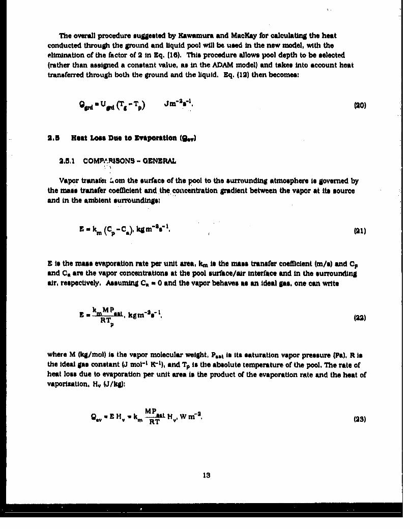
The overall procedure suggested by Kawamura and MacKay for calculating the heatconducted through the ground and liquid pool will be used in the new model, with theelimination of the factor of 2 in Eq. (16). This procedure allows pool depth to be selected(rather than assigned a constant value, as in the ADAM model) and takes into account heattransferred through both the ground and the liquid. Eq. (12) then becomes:

Ql2d a Ur (TS1 Tp) .Jm " T 5o (20)

2.5 Heat Loes Due to Evaporation (.,)

2.5.1 COMPARISONS - GENERAL

Vapor transtez £ am the surface of the pool to the surrounding atmosphere is governed bythe mass transfer coefficient and the concentration gradient between the vapor at its sourceand in the ambient surrounding*:

E a km (Cp-CA), kgm-s'4 1 . (21)

E is the mass evaporation rate per unit area, km is the mass transfer coefficient (m/s) and Cpand Ca are the vapor concentrations at the pool surface/air interface and in the surroundingair, respectively. Assuming Ca m 0 and the vapor behaves as an ideal gas, one can write

k MP -- 1E w -M--sai, kg t s'a (22)

where M (kg/mol) Is the vapor molecular weight, P,, is Its saturation vapor pressure (Pa), R Isthe Ideal gas constant (J mol-I W-), and Tp is the absolute temperature of the pool. The rate ofheat loss due to evaporation per unit area is the product of the evaporation rate and the heat ofvaporization, Hv (J/kg):

96RT ZHv W M'O (23)

13

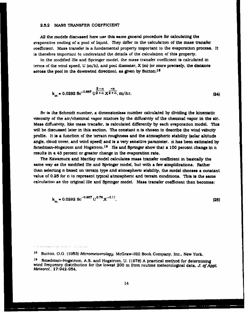
2.5.2 MASS TRANSFER COEFFICIENT

All the models discussed here use this same general procedure for calculating theevaporative cooling of a pool of liquid, They differ in the calculation of the mass transfercoefficient. Mass transfer is a fundamental property important to the evaporation process. Itis therefore important to understand the details of the calculation of this property.

In the modified ille and Springer model, the mass transfer coeflfcient is calculated interms of the wind speed, U (m/h), and pool diameter, X (m) (or more precisely, the distanceacross the pool in the downwind direction), as given by Sutton:16

2-n -nkm = 0.0292 Sc"°'00 " U2 +n X2 ÷ n, m/hr. (24)

Sc is ihe Schmidt number, a dimensionless number calculated by dividing the kinematicviscosity of the air/chemical vapor mixture by the dliffusivity of the chemical vapor in the air.Mass diffusivity, like mass transfer, is calculated differently by each evaporation model, Thiswill be discussed later in this section. The constant n is chosen to describe the wind velocityprofile, It is a function of the terrain roughness and the atmospheric stability (solar altitudeangle, cloud cover, and wind speed) and is a very sensitive parameter, n has been estimated bySinedman-Hogstrom and Hogstrom,19 Ille and Springer show that a 100 percent change in nresults In a 43 percent or greater change in the evaporation rate,

The Kawamura and MacKay model calculates mass transfer coe/icient in basically thesame way as the modified flle and Springer model, but with a few simplifications, Ratherthan selecting n based on terrain type and atmospheric stability, the model chooses a constantvalue of 0.25 for n to represent typical atmospheric and terrain conditions. This is the samecalculation as the original flle and Springer model, Mass transfer coefficient then becomes:

km a 0,0292 Sc- 0 a U°'? X°. (25)

ISSutton, 0.0, (1953) Micrometeorology, McGraw-i-fll Book Company, Inc., New York.IV Smedman-Hogstrom, A,S. and Hogutrom, U, (1978) A practical method for determiningwind frequency distrilbution for the lowest 200 m from routine meteorological data, J. of AppLMeteorol., 17:942-954.

14

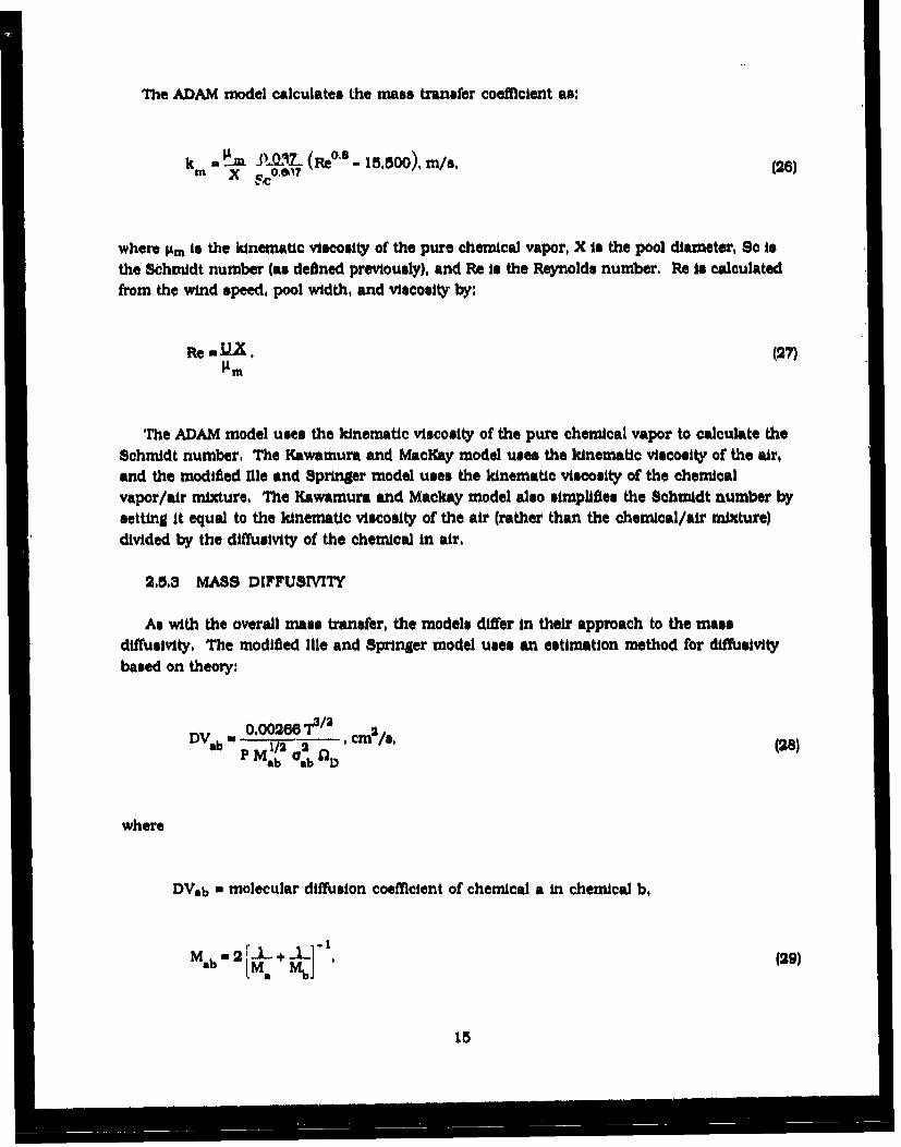
The ADAM model calculates the mass transfer coefficient as:

km • JQL3_ (Re", - 15,500), m/s, (26)m X E!o .017 "(

where gm is the kinematic viscosity of the pure chemical vapor, X is the pool diameter, Sc isthe Schmidt number (as defined previously), and Re is the Reynolds number. Re is calculatedfrom the wind speed, pool width, and viscosity by:

Reu- X, (27)

The ADAM model uses the kinematic viscosity of the pure chemical vapor to calculate theSchmidt number, The Kawamura and MacKay model uses the kinematic viscosity of the air,and the modified Ille and Springer model uses the kinematic viscosity of the chemicalvapor/air mixture. The Kawamura and Mackay model also simplifies the Schmidt number by

setting it equal to the kinematic viscosity of the air (rather than the chemical/air mixture)divided by the diffusivity of the chemical in air.

2.5.3 MASS DIFFUSIVITY

As with the overall mass transfer, the models differ in their approach to the massdiffusivity. The modified Ille and Springer model uses an estimation method for diffusivitybased on theory:

DVab- 0.002e6 703/2 eS/s(bPM11 t/ ,cm/s (28)ab ab 1)

where

DV-b a molecular diffusion coefflcient of chemical a In chemical b,

Mab '2 [- + (29)

15

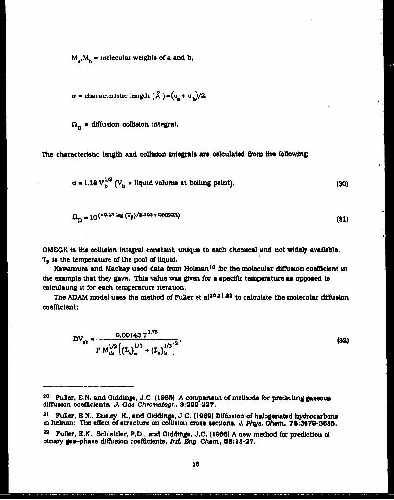
Ma Mb - molecular weights of a and b,

a - characteristic length (A) + /

OD a diffusion collision integral,

The characteristic length and collision integrals are calculated from the following:

1 /3

O 1.18 Vb (Vb = liquid volume at boiling point), (30)

*D l0(-0". log (Tp)/2,3 ÷+oGMEOK), (31)

OMEGK is the collision integral constant, unique to each chemical and not widely available.Tp is the temperature of the pool of liquid.

Kawamura and Mackay used data from Holman"3 for the molecular diffusion coefficient inthe example that they gave. This value was given for a specific temperature as opposed tocalculating it for each temperature iteration,

The ADAM model uses the method of Fuller et al2 0 .2 1 ,22 to calculate the molecular diffusion

coefficient:

DV~ a.- 00143 T1 75

PM.1 2 [((E)!I3 + I/3"-b b

20 Fuller, E,N, and Giddings, JC. (1965) A comparison of methods for predicting gaseousdiffusion coefficients, J. Gas Chromatogr., 8:222-227.21 Fuller, E.N,, Ensley, K., and Giddings, J C. (1969) Diffusion of halogenated hydrocarbonsin helium: The effect of structure on collision crons sections, J, Phiys. Chem., 7,:3079-3685.22 Fuller, E.N., Schlettler, P.DA, and Giddings, J.C. (1966) A new method for prediction ofbinazy gas-phase diffusion coefficients, Ind, MV. Chem., 58:18-27.

16

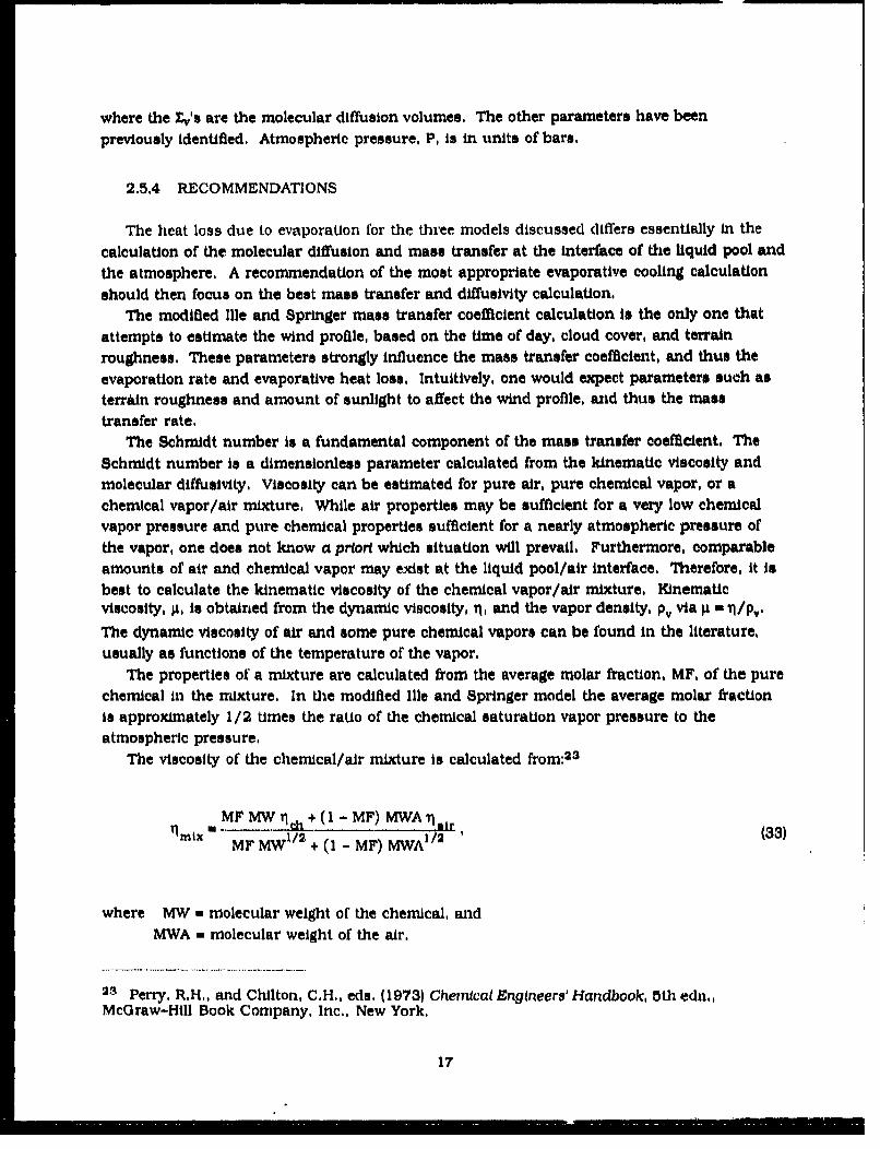
where the 4~'s are the molecular diffusion volumes. The other parameters have been

previously identified. Atmospheric pressure, P, is in units of bars,

2.5.4 RECOMMENDATIONS

The heat loss due to evaporation for the three models discussed differs essentially in the

calculation of the molecular diffusion and mass transfer at the interface of the liquid pool and

the atmosphere. A recommendation of the most appropriate evaporative cooling calculation

should then focus on the best mass transfer and diffusivity calculation.The modified Ille and Springer mass transfer coefficient calculation is the only one that

attempts to estimate the wind profile, based on the time of day, cloud cover, and terrainroughness, These parameters strongly influence the mass transfer coefficient, and thus theevaporation rate and evaporative heat loss, Intuitively, one would expect parameters such asterrain roughness and amount of sunlight to affect the wind profile, and thus the mass

transfer rate,The Schmidt number is a fundamental component of the mass transfer coefficient. The

Schmidt number is a dimensionless parameter calculated from the kinematic viscosity andmolecular diffusivity, Viscosity can be estimated for pure air, pure chemical vapor, or achemical vapor/air mixture, While air properties may be sufficient for a very low chemicalvapor pressure and pure chemical properties sufficient for a nearly atmospheric pressure ofthe vapor, one does not know a priori which situation will prevail. Furthermore, comparableamounts of air and chemical vapor may exist at the liquid pool/air interface. Therefore, it isbest to calculate the kinematic viscosity of the chemical vapor/air mixture. Kinematicviscosity, g, is obtained from the dynamic viscosity, rl, and the vapor density, p. via g n t*/Pv.

The dynamic viscosity of air and some pure chemical vapors can be found in the literature,usually as functions of the temperature of the vapor.

The properties of a mixture are calculated from the average molar fraction, MF, of the purechemical in the mixture, In the modified Ille and Springer model the average molar fractionis approximately 1/2 times the ratio of the chemical saturation vapor pressure to theatmospheric pressure,

The viscosity of the chemical/air mixture is calculated from:2 3

MF MW th + (I - MF) MWA irflU - (33)mix MF MWI12'+ (I - MF) MWA 1 '2 (33)

where MW w molecular weight of the chemical, andMWA w molecular weight of the air.

23 Perry, RH,, and Chilton, CH,, eds. (1973) Chemical Engineers' Handbook, 5th edn.,McGraw-Hill Book Company, Inc., New York,

17

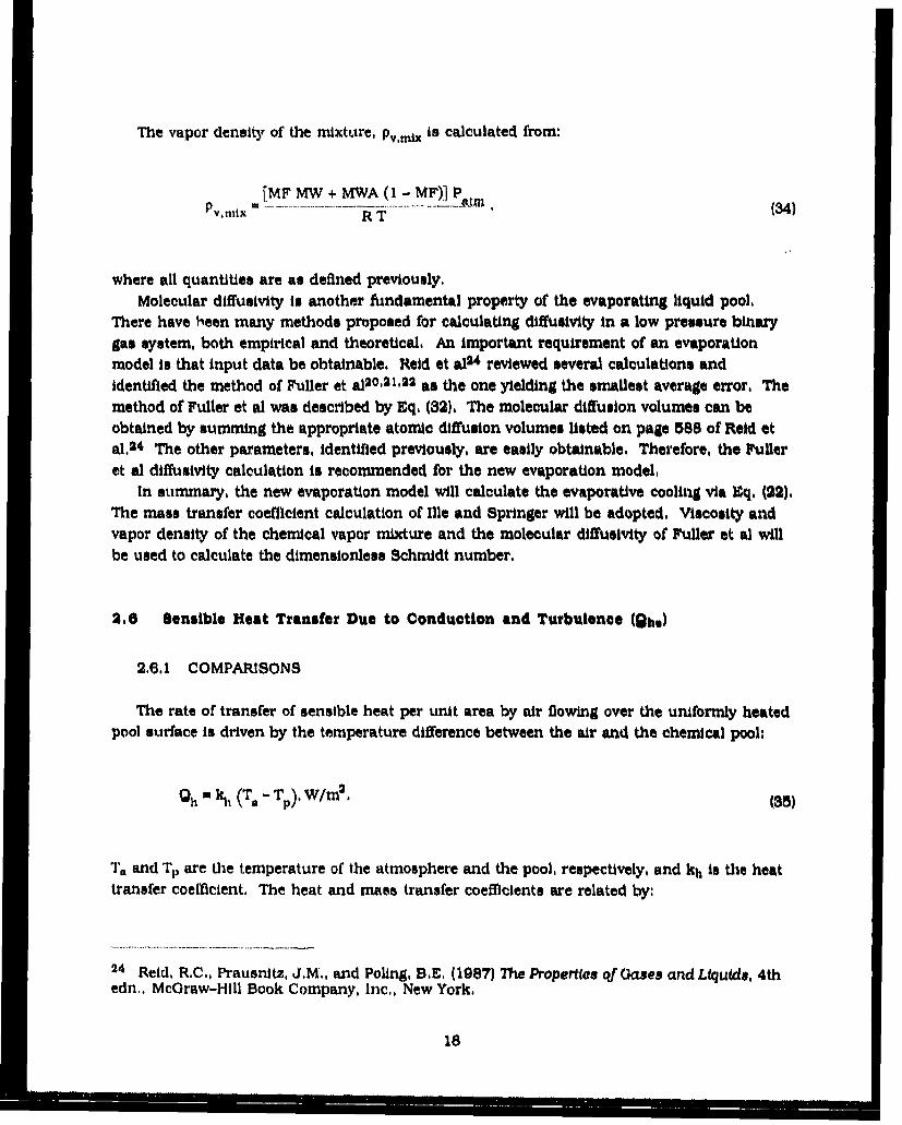
The vapor density of the mixture, Pv,mix is calculated from:

[MF MW + MWA (I - MF)] PPv,tx= RT , (34)

where all quantities are as defined previously.Molecular diffusivity is another fundamental property of the evaporating liquid pool,

There have been many methods proposed for calculating diffusivity in a low pressure binarygas system, both empirical and theoretical. An important requirement of an evaporationmodel is that input data be obtainable. Reid et as24 reviewed several calculations andidentified the method of Fuller et al2 0 .2 1, 2 2 as the one yielding the smallest average error, Themethod of Fuller et al was described by Eq. (32), The molecular diffusion volumes can beobtained by summing the appropriate atomic diffusion volumes listed on page 588 of Reid etal.2 4 The other parameters, identified previously, are easily obtainable. Therefore, the Fulleret al diffusivity calculation is recommended for the new evaporation model,

In summary, the new evaporation model will calculate the evaporative cooling via Eq. (22).The mass transfer coefficient calculation of Ille and Springer will be adopted, Viscosity andvapor density of the chemical vapor mixture and the molecular diffusivity of Fuller et al willbe used to calculate the dimensionless Schmidt number.

2,6 Sensible Heat Transfer Due to Conduction and Turbulence (Bh,)

2.6.1 COMPARISONS

The rate of transfer of sensible heat per unit area by air flowing over the uniformly heatedpool surface is driven by the temperature difference between the air and the chemical pool:

Gh= (T1 - TP). W/m 2 . (35)

Ta and Tp are the temperature of the atmosphere and the pool, respectively, and kh is the heattransfer coefficient. The heat and mass transfer coefficients are related by:

24 Reid, R.C., Prausnltz, J.M., and Poling, B.E, (1987) The Properties of Oases and Liquids, 4thedn., McGraw-Hill Book Company, Inc,, New York.

18

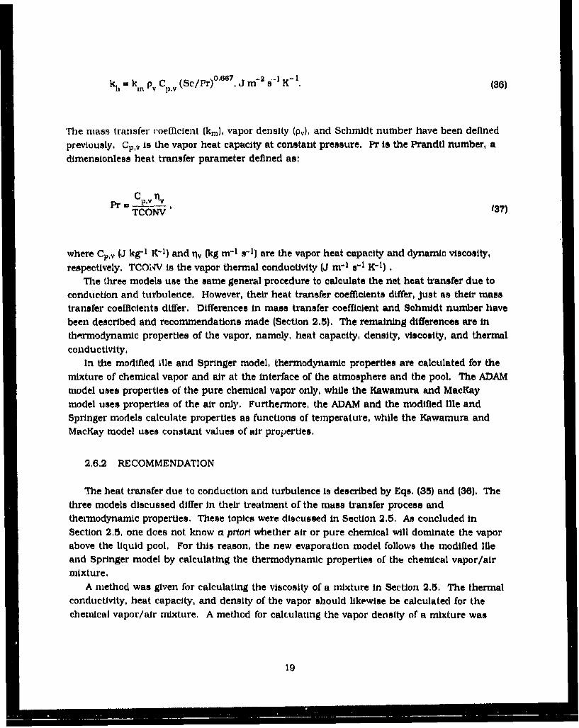
k 1 = k M Pv Cp'v (Sc/Pr)'s 7 J M-2am s'- K- 1 ' (36)

The mass transfer coefficient (km), vapor density (pv), and Schmidt number have been defined

previously. Cp,v is the vapor heat capacity at constant pressure. Pr is the Prandtl number, a

dimensionless heat transfer parameter defined as:

Pr - C"'v 137

TCONV' (37)

where Cpv (J kg-1 K-1 ) and nv (kg m-1 s-1 ) are the vapor heat capacity and dynamic viscosity,

respectively. TC01'V is the vapor thermal conductivity (J m-1 sa- K71) .

The three models use the same general procedure to calculate the net heat transfer due to

conduction and turbulence. However, their heat transfer coefficients differ, just as their masstransfer coefficients differ. Differences in mass transfer coefficient and Schmidt number have

been described and recommendations made (Section 2.5). The remaining differences are in

the'rmodynamic properties of the vapor, namely, heat capacity, density, viscosity, and thermal

conductivity,In the modified WUe arid Springer model, thermodynamic properties are calculated for the

mixture of chemical vapor and air at the interface of the atmosphere and the pool. The ADAM

model uses properties of the pure chemical vapor only, while the Kawamura and MacKay

model uses properties of the air only. Furthermore, the ADAM and the modified Ille and

Springer models calculate properties as functions of temperature, while the Kawamura andMacKay model uses constant values of air properties.

2,6.2 RECOMMENDATION

The heat transfer due to conduction and turbulence is described by Eqs. (35) and (36). The

three models discussed differ in their treatment of the mass transfer process and

thermodynamic properties. These topics were discussed in Section 2.5, As concluded in

Section 2.5, one does not know a plorl whether air or pure chemical will dominate the vapor

above the liquid pool. For this reason, the new evaporation model follows the modified Ille

and Springer model by calculating the thermodynamic properties of the chemical vapor/air

mixture.A method was given for calculating the viscosity of a mixture in Section 2.5. The thermal

conductivity, heat capacity, and density of the vapor should likewise be calculated for the

chemical vapor/air mixture. A method for calculating the vapor density of a mixture was

19

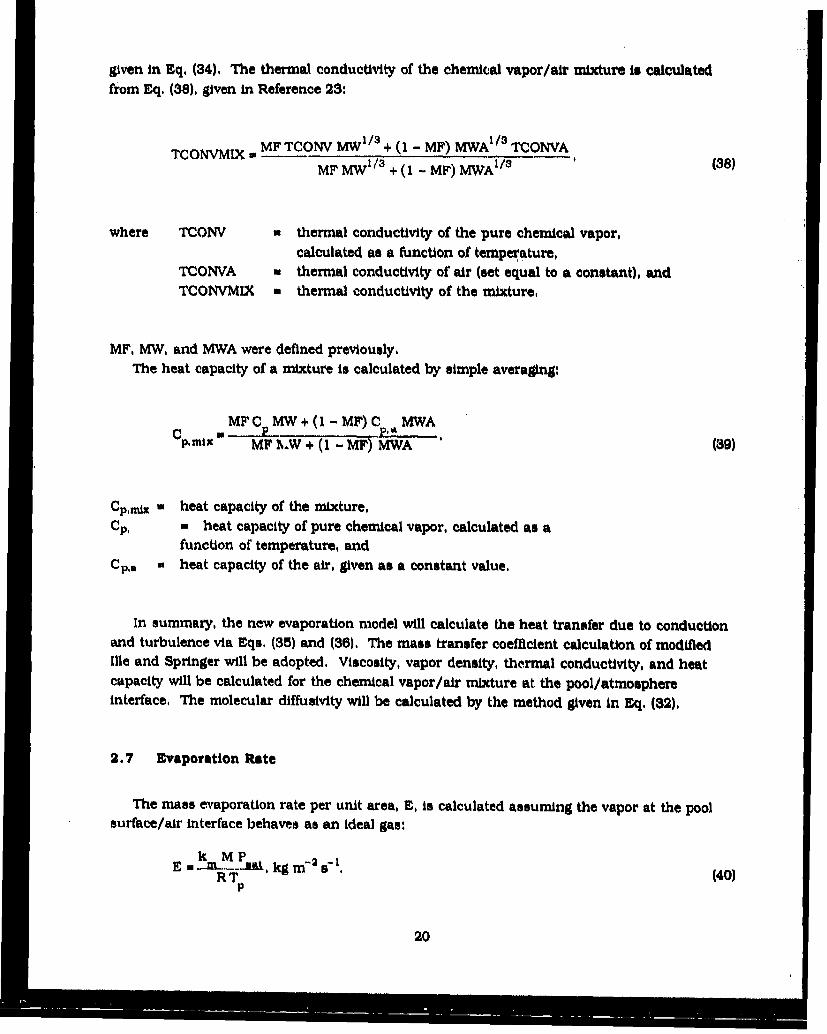
given in Eq. (34), The thermal conductivity of the chemical vapor/air mixture is calculatedfrom Eq. (38), given in Reference 23:

TCNVMIX =MF TCONV MW1/3 + (1 - MF) MWA1 /3 TCONVA

MF MWI/3 + (1 - MF) MWA 1/3 ' (38)

where TCONV a thermal conductivity of the pure chemical vapor,calculated as a function of temperature,

TCONVA a thermal conductivity of air (set equal to a constant), andTCONVMIX w thermal conductivity of the mixture,

MF, MW, and MWA were defined previously,The heat capacity of a mixture is calculated by simple averaging:

MFC MW+(I-MF) C MWAP.Mix MF h.W + (I - MF) MWA (89)

Cp,nix a heat capacity of the mixture,CP, = heat capacity of pure chemical vapor, calculated as a

function of temperature, andCp,A - heat capacity of the air, given as a constant value,

In summary, the new evaporation model will calculate the heat transfer due to conductionand turbulence via Eqs. (35) and (36). The mass transfer coefficient calculation of modifiedIlle and Springer will be adopted. Viscosity, vapor density, thermal conductivity, and heatcapacity will be calculated for the chemical vapor/air mixture at the pool/atmosphereinterface, The molecular diffusivity will be calculated by the method given in Eq, (32),

2.7 Evaporation Rate

The mass evaporation rate per unit area, E, is calculated assuming the vapor at the poolsurface/air interface behaves as an ideal gas:

_AM. ikgnrIf2 e 1RT (40)

20

km.. the mass transfer coefficient (m/s), is calculated as in Eq. (24) and Is a function of pooltemperature, Tp. The saturation vapor pressure of the chemical, P,,t (Pa), is also a function ofthe pool temperature via the Antoine equation:16

log P*at p (41)

where A, B, and C are constants unique to each chemical.To get the overall evaporation rate in kg/s, Eq. (40) is multiplied by the surface area, A, of

the pool. In the modified Ille and Springer and tho Kawamura and MacKay models, the area isInput by the user. In the ADAM model it Is calculated from the volume of chemical spilled,assuming a pool depth of I cm.

2.8 Calculation of Liquid Chemical Pool Temperature

Many of the energy terms comprising Eq, (1), the steady state energy balance, can beexpressed as functions of the pool temperature. The evaporation models solve for the pooltemperature using the Newton-Raphson Iterative procedure.

3. SUMMARY OF THE NEW EVAPORATION MODEL

In the previous section, three steady state energy balance evaporation models for a pool ofspilled liquid chemical were compared and evaluated. A new evaporation model was proposedbased on these evaluations, In this section, a summary of the new evaporation model ispresented. The new model is a composite of the three models reviewed in Section 2.

Table 3 shows the input data required for each model.

21

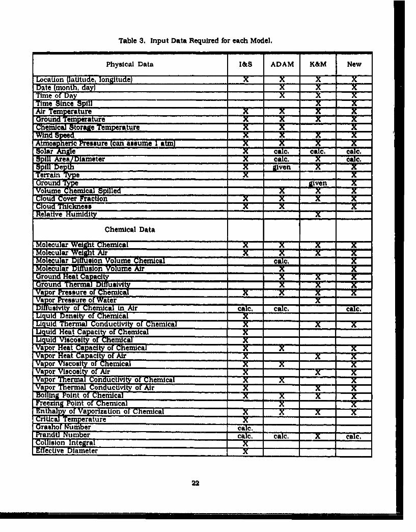
Table 3. Input Data Required for each Model.

Physical Data I&S ADAM K&M New

Location (latitude, longitude) ... X X X.Date (month, day) x XTime of Day . . , X xTime Since Spill x ,.. TAir Temperature x X T TGround Temperature xChermical Storage Temperature X X".Wind Speed, I , X, xAtmospheric Pressure (can assume I atm) , n- -- = "w" =

Solar Angle X.... c-a le, calc, c alc,

$pill Area/Diameter MXi .le. Cale,SPill Depth ... X gie xTerrain Type X XGround -Tg• givnVolume chemical x led X xCloud Cover Fraction x'. x x XCloud Thickness x XRelative Humdit x

Chemical Data

Molecular ei emical, X x "" x xMolrecular Wei~ht Air x, _' _ -2Molecular Diffusion Volume Chemical cabIc. XMolecular Diffusion Volume Air XGround Heat apaca xGround Thermal Diffusivity x x 'Vapor Pressure of Chemical x x . h XVapor Pressure of Water -.- x

iuslvty of Che mcal in Air ClA. talc, calc,Liquid Density of Chemical XLiquid Thermal Conductivi o Chemical X _ _ , XLiquid Heat Capacity of Chen-xcal XLiquid Viscosity of Chemica~l -xVapor Heat Capacity of Cemical x " XVapor Heat Capaclt of Ar...X.. .. x"Vapor viscosit of Chemical .. ' X, 'x

apor Vlscost of Air XX -XVapor Thermal conductity of chemical x ____x_

Vapor Thermal Conductivity of Air .. X XBoiling Point of Chemical x.. " X X XFreezing Point of Chemical XEnthalpy of Vaporization of Chemical .X T X XCritical Temperature . .x ....drashof Number 'Cale.PrandUo Number cale, calc, *X ca=c,

Collision Integral X__"Effective Diameter X

22

These data are supplied by separate chemical data files and by user input during programexecution. The modified Ille and Springer model and the new model require the mostchemical data. Unavailability of chemical data may limit the use of theme models.

All of the models reviewed and the one proposed are steady state energy balanceevaporation models. A steady state energy balance evaporation model is one in which the sumof all sources of energy (heat) transported into the pool exactly balances the sum of energysources transported out of the pool. Many of these sources of energy can be expressed in termsof the liquid chemical pool temperature, which is calculated iteratively, That calculatedtemperature is used to calculate the evaporation rate,

The steady state energy balance is expressed as:

Qs+ +atm + p• h + hev + 0.rd (42)

Terms of this equation were defined in Section 1 and described in detail in Section 2,Calculations for the new model are summarized below,

3.1 Heat Due to Net Solar Radiation

The net heat due to solar radiation reaching the spilled liquid depends on the angle of thesun with respect to the pool and the amount and type of cloud cover. The solar altitude angle,SA, is calculated using an equation from Reference 5:

sin SA - sin LA sin D + cos LA cos D cos SHA. (43)

LA is the geographical latitude of the pool, D is the solar declination, and SHA is the solarhour angle,

The heat from the net solar radiation is calculated as in the ADAM model:

Q001 M RS (I - alb), W/m 2 . (44)

The liquid pool albedo, alb, is included to correct for solar radiation reflected away from thepool. The net radiation per unit area, RS, Is calculated from the following:S-9 iO

23

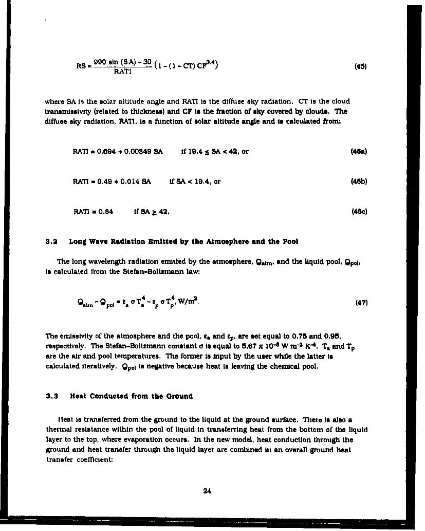
RS 990 sin (SA) - 30 (1 - (I - CT) Cp3'4 ) (45)RATI

where SA Is the solar altitude angle and RATI is the diffuse sky radiation. CT is the cloudtransmissivity (related to thickness) and CF is the fraction of sky covered by clouds. Thediffuse sky radiation, RATI, is a function of solar altitude angle and to calculated from:

RATI a 0,694 + 0.00349 SA if 19.4 S SA - 42, or (46a)

RAT! . 0.49 + 0,014 SA if SA < 194, or (46b)

RATM 0.84 if SA ?. 42, (46c)

8,2 Long Wave Radiation Emitted by the Atmosphere and the Pool

The long wavelength radiation emitted by the atmosphere, Q..t, and the liquid pool, Qpol,is calculated from the Stefan-Boltzmann law:

941s - mP0l a e AT4- eP oT'P4, W/m2. (47)

The emissivity of the atmosphere and the pool, ta. and ep, are set equal to 0.75 and 0.95,respectively, The Stefan-Boltznann constant a is equal to 5.67 x 10-8 W m-2 K-4. Ta and Tpare the air and pool temperatures. The former is input by the user while the latter iscalculated iteratively. Qp.1 is negative because heat is leaving the chemical pool,

3.3 Heat Conducted from the Ground

Heat is transferred from the ground to the liquid at the ground surface. There is also athermal resistance within the pool of liquid in transferring heat from the bottom of the liquidlayer to the top, where evaporation occurs. In the new model, heat conduction through theground and heat transfer through the liquid layer are combined in an overall ground heattransfer coefficient:

24

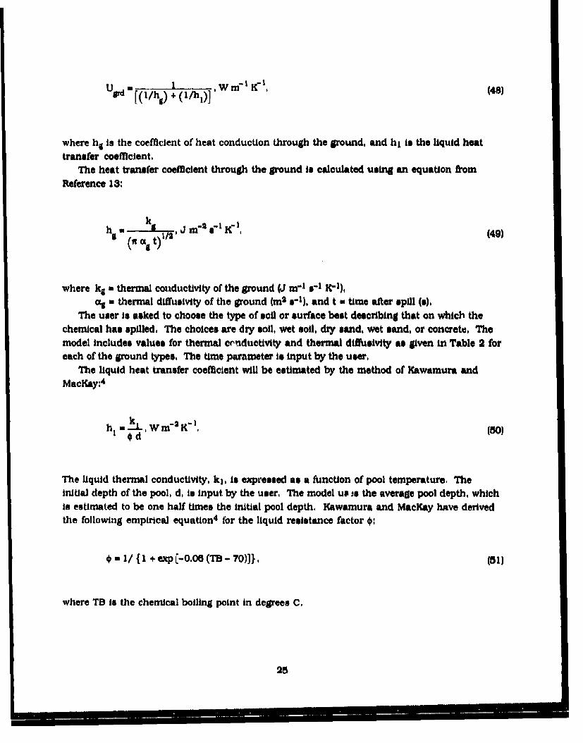
Ugt W m -K (48)S[(/hg) + (1/h)] m- K-

where ha is the coefficient of heat conduction through the ground, and hl is the liquid heattransfer coefficient.

The heat transfer coefficient through the ground is calculated using an equation flromReference 13:

Sh k k

(ha ag t)

where kga thermal conaductivity of the ground (J m-1 sI K-1),

a. thermal diffusivity of the ground {m2 V1 ), and t m time after spill (s)The user is asked to choose the type of soil or surface best describing that on which the

chermical has spilled. The choices are dry soil, wet soil, dry sand, wet sand, or concrete, Themodel includes values for thermal cpnductivity and thermal diffusivity as given in Table 2 foreach of the ground types, The time parameter Is input by the user,

The liquid heat transfer coefficient will be estimated by the method of Kawamura andMacKay:4

hi = kd. W m-2 K-'. (50)

The liquid thermal conductivity, ki, is expressed as a function of pool temperature, TheInitial depth of the pool, d, is input by the user, The model ut ts the average pool depth, whichis estimated to be one half times the initial pool depth, Kawamura and MacKay have derivedthe following empirical equation 4 for the liquid resistance factor *:

* = I/ { I + exp [-006 (TB - 70)]}. (51)

where TB is the chemical boiling point in degrees C.

25

8.4 Heat Lose Due to Nvaporatlon 2

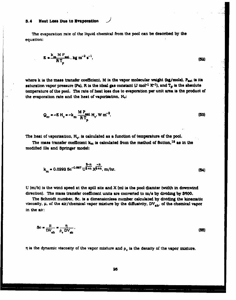
The evaporation rate of the liquid chemical from the pool can be described by theequation:

Ea IM kgw 2p (5)

where k is the mass transfer coefficient, M is the vapor molecular weight (kg/mole), Post Is itssaturation vapor pressure (Pa), R Is the ideal gas constant (J reolI K-l), and Tp is the absolutetemperature of the pool. The rate of heat Igoe due to evaporation per unit area is the product ofthe evaporation rate and the heat of vaporliation, Hv:

GIV a -E+ Hv a -km M stp Hv, W m -2 aSS)MTP

The heat of vaporization, Nv, is calculated as a function of temperature of the pool.The mass transfer coeficent km is calculated from the method of Sutton, 1I as in the

modified Ill© and Springer model:

2-n -nkm 0,0 2 9 2 SC"1"0 e7 Ul+n X2+", m/hr, (54)

U (m/h) is the wind speed at the spill site and X (m) is the pool dlamter (width in downwinddirection). The mass transfer coeffcient units are converted to w/s by dividing by 8600.

The Schmidt number, Sc, is a dimensionless number calculated by dividing the kinematicviscosity, pI, of the air/chemical vapor mixture by the diflusivlty, DVWb, of the chemical vapor

in the air:

Sc. * _ -__ S,"'VVb P, DVb (55)

tj is the dynamic viscosity of the vapor mixture and p. is the density of the vapor mlxture,

28

The mass diflusivity of the chemical vapor in air is calculated by the method of auller et

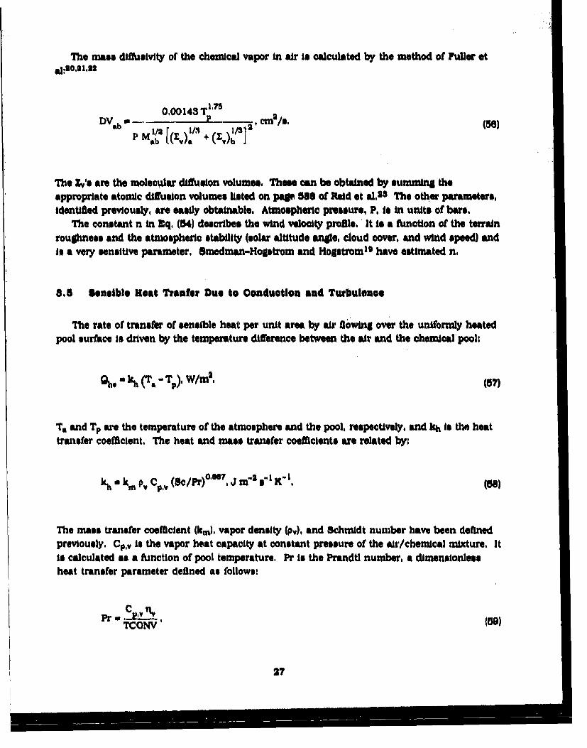
000143 T IDVab 2 P2cm2/s.

'b'2~ ~ kt) OM

The Zv's are the molecular diffusion volume, These can be obtained by summin theappropriate atomic diffusion volumes listed on pW 588 of Reid et aL5 3 The other parameters,identified previously, are easily obtainable. Atmospheric pressure, P, to in units of bar*.

The constant n in Eq, (54) describes the wind velocity profile. It is a function of the terrainroughness and the atmospherio stability (solar altitude anle, cloud cover, and wind speed) andis a very sensitive parameter. Smedman-Hogstrom and Hogstrom 19 have estimated n,

8,5 Sensible Heat Tranfer Due to Conduction and Turbulence

The rate of transfer of sensible heat per unit area by ala' flowing over the uniformly heatedpool surface is driven by the temperature difference between the air and the chemical pool:

0 h. = kh (xw T OWmf , (5/7)

T. and Tp are the temperature of the atmosphere and the pool, respectively, and kh Is the heattransfer coefficient, The heat and mass transfer coefficients are related by:

kh C km pv CpV (Sc/Pr)°'66 7 Jm'sa -I X-I, (08)

The mass transfer coefficient (km), vapor density (p,), and Schmidt number have been definedpreviously. Cp,, is the vapor heat capacity at constant pressure of the .1:/chemical mixture, Itis calculated as a function of pool temperature, Pr is the Prandtl number, a dimensionlessheat transfer parameter defined as follows:

TCONV

27

where Cp,v (J kg-I1 K-1 ) and qv (kg ra-1 s1) are the vapor heat capacity and dynamic viscosity,respectively. TCONV is the vapor thermal conductivity VJ m-I s-I K-1). Each of thesethermodynamic parameters is a function of the pool temperature.

Note that when the pool is warmer than the air there will be a loss of heat from the pool bythis heat transfer mode, and the calculated sensible heat flux into the pool will be negative.

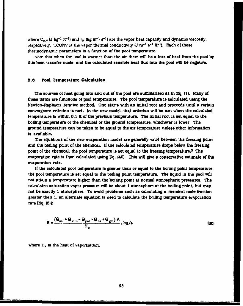
8.6 Pool Temperature Calculation

The sources of heat going into and out of the pool are summarized as in Eq, (1). Many ofthese terms are functions of pool temperature, The pool temperature ts calculated using theNewton-Raphson iterative method. One starts with an initial root and proceeds until a certainconvergence criterion is met, In the new model, that criterion will be met when the calculatedtemperature is within 0, 1 K of the previous temperature, The initial root is set equal to theboiling temperature of the chemical or the ground temperature, whichever Is lower, Theground temperature can be taken to be equal to the air temperature unless other Informationis available,

The equations of the new evaporation model are generally valid between the freezing pointand the boiling point of the chemical. If the calculated temperature drops below the freezingpoint of the chemical, the pool temperature is set equal to the freezing temperature.3 Theevaporation rate is then calculated using Eq. (40). This will give a conservative estimate of theevaporation rate.

If the calculated pool temperature is greater than or equal to the boiling point temperature,the pool temperature is set equal to the boiling point temperature, The liquid in the pool willnot attain a temperature higher than the boiling point at normal atmospheric pressures. Thecalculated saturation vapor pressure will be about I atmosphere at the boiling point, but maynot be exactly I atmosphere. To avoid problems such as calculating a chemical mole fractiongreater than 1, an alternate equation is used to calculate the boiling temperature evaporationrate [Eq, (3)1:

E hat " d) 9, Pot (+0)

where Hv It the heat of vaporization.

28

3.7 Chemical Data Base

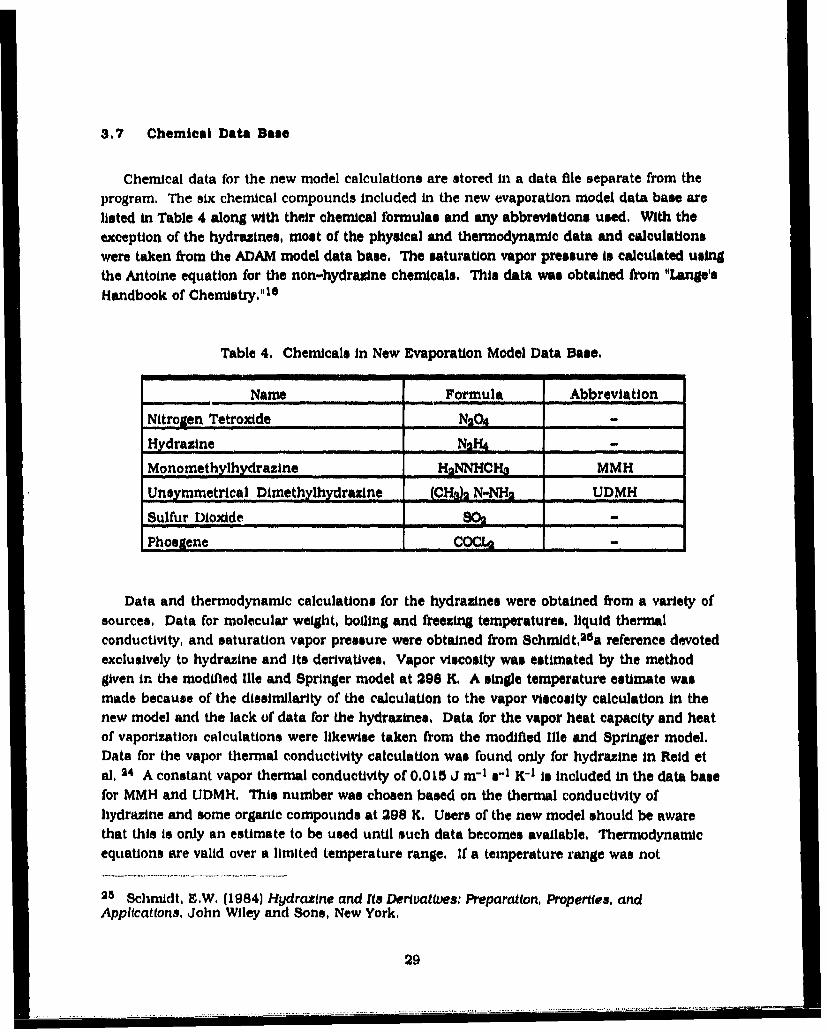
Chemical data for the new model calculations are stored in a data file separate from theprogram, The six chemical compounds included in the new evaporation model data base arelisted in Table 4 along with their chemical formulas and any abbreviations used, With theexception of the hydrazines, most of the physical and thermodynamic data and calculationswere taken from the ADAM model data base. The saturation vapor pressure is calculated usingthe Antoine equation for the non-hydrazine chemicals, This data was obtained from "Lange'sHandbook of Chemlstry."le

Table 4. Chemicals In New Evaporation Model Data Base,

Name Formula Abbreviation

Nitrogen Tetroxide N20 4 -

Hydratine N4!/ -

Mono methylhydrazine H2NNHCH- MMH

Unsymmetrical Dimethylhydraxine (CHa)2 N-NH2 UDMH

Sulfur Dioxide S02_- _i

Phosgene .COCL

Data and thermodynamic calculations for the hydrazines were obtained from a variety ofsources, Data for molecular weight, boiling and freezing temperatures, liquid thermalconductivity, and saturation vapor pressure were obtained from Schmidt, 25 a reference devotedexclusively to hydrazine and its derivatives. Vapor viscosity was estimated by the methodgiven in the modified Ille and Springer model at 298 K. A single temperature estimate wasmade because of the dissimilarity of the calculation to the vapor viscosity calculation In thenew model and the lack of data for the hydrazines, Data for the vapor heat capacity and heatof vaporization calculations were likewise taken from the modified Jlle and Springer model.Data for the vapor thermal conductivity calculation was found only for hydrazine in Reid etal. 24 A constant vapor thermal conductivity of 0.015 J m-1 s-1 K-1 is included in the data basefor MMH and UDMH. This number was chosen based on the thermal conductivity ofhydrazine and some organic compounds at 298 K. Users of the new model should be awarethat this Is only an estimate to be used until such data becomes available, Thermodynamicequations are valid over a limited temperature range. If a temperature range was not

25 Schmidt, E.W, (1984) Hydraztne and [is Derivatives: Preparation, Properties, andApplications, John Wiley and Sons, New York,

29

available, the freezing point and boiling points are used as the lower and upper bounds of therange of valid temperatures.

4. NEW MODEL SENSITIVITY STUDIES

In the previous sections, a new evaporation model was developed based on the evaluationof three existing evaporation models - the modified llle and Springer model, the ADAM model,and the Kawamura and MacKay model. In this section, sensitlvity studies of the new modelare presented in support of the recommendations of the previous sections,

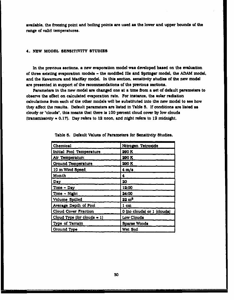
Parameters in the new model are changed one at a time from a set of default parameters toobserve the effect on calculated evaporation rate. For instance, the solar radiationcalculations from each of the other models will be substituted into the new model to see howthey affect the results. Default parameters are listed in Table 5. If conditions are listed ascloudy or "clouds", this means that there is 100 percent cloud cover by low clouds(transmlssivity w 0,17), Day refers to 12 noon, and night refers to 12 midnight.

Table 5. Default Values of Parameters for Sensitivity Studies,

Chemical Nitrogen TetrocideInitial Pool Temperature 290 KAir Temperatur. 290 K

Ground Temperature 290 K10 m Wind Speed 4 m/,Month 4Day 20

Time - Day 12:00Time - Night 24:00

Volume Spilled 22 ms

Average Depth of Pool I cmCloud Cover Fraction 0 (no clouds) or I (clouds)

Cloud TYpe (for clouds , 1) Low CloudsType of Terrain Sparse WoodsGround Type Wet Soil

30

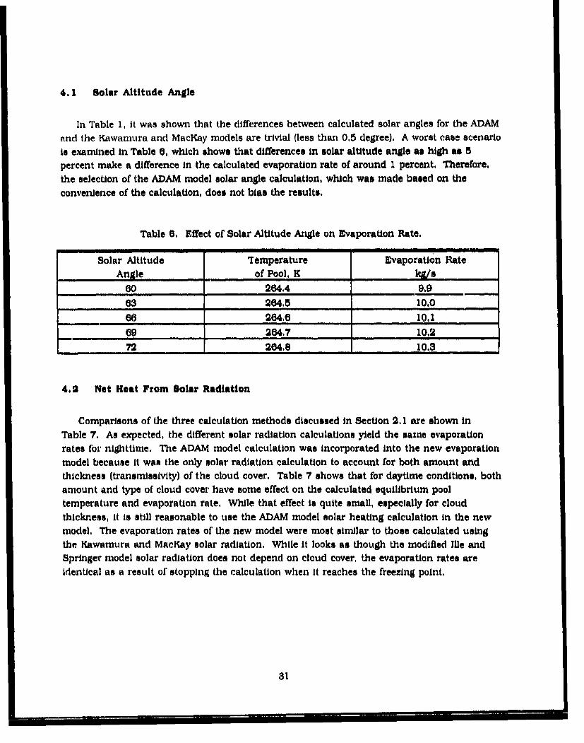
4.1 Solar Altitude Angle

In Table 1, it was shown that the differences between calculated solar angles for the ADAMand the Kawamura and MacKay models are trivial (less than 0.5 degree). A worst case scenario

is examined in Table 6, which shows that differences in solar altitude angle as high as 5percent make a difference in the calculated evaporation rate of around I percent. Therefore,

the selection of the ADAM model solar angle calculation, which was made based on theconvenience of the calculation, does not bias the results.

Table 8, Effect of Solar Altitude Angle on Evaporation Rate,

Solar Altitude 'Temperature Evaporation Rate

Angle of Pool, K kg/s

60 264.4 9.963 264,5 10.0

66 264.6 10,1

69 264.7 10.2

72 264.8 10.3

4.2 Net Heat From Solar Radiation

Comparisons of the three calculation methods discussed in Section 2.1 are shown in

Table 7. As expected, the different solar radiation calculations yield the same evaporationrates for nighttime. The ADAM model calculation was incorporated into the new evaporationmodel because it was the only solar radiation calculation to account for both amount andthickness (transmissivity) of the cloud cover. Table 7 shows that for daytime conditions, both

amount and type of cloud cover have some effect on the calculated equilibrium pooltemperature and evaporation rate. While that effect is quite small, especially for cloud

thickness, it is still reasonable to use the ADAM model solar heating calculation in the newmodel. The evaporation rates of the new model were most similar to those calculated using

the Kawamura and MacKay solar radiation. Wlhile it looks as though the modified hlle andSpringer model solar radiation does not depend on cloud cover, the evaporation rates areidentical as a result of stopping the calculation when it reaches the freezing point.

31

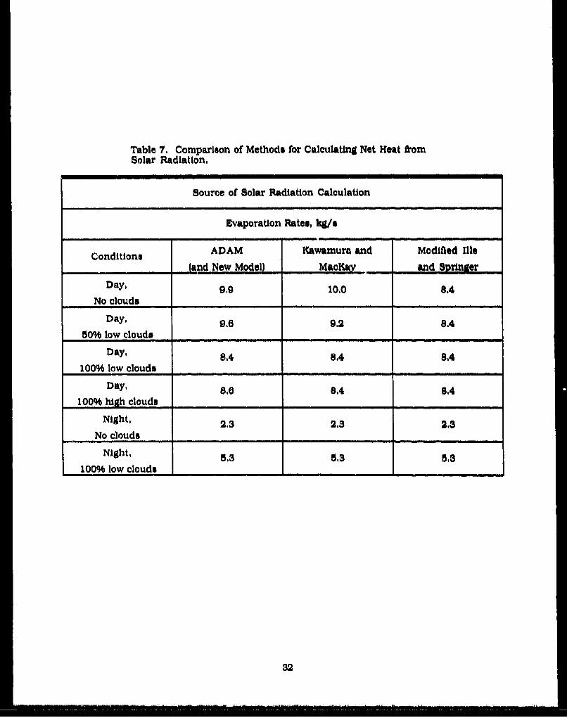
Table 7. Comparison of Methods for Calculating Net Heat ftom

Solar Radiation,

Source of Solar Radiation Calculation

Evaporation Rates, kg/s

Conditions ADAM Kawamura and Modified Ills

land New Model) MacKay and Springer

Day, 9,9 10.0 8.4

No clouds

Day, 9.6 9.2 8.4

50% low clouds ......

Day, 8.4 8.4 8.4

100% low clouds

Day, 8.1 8.4 8.4

100% high clouds

Night, 2.3 2.3 2.3

No clouds

Night, 5.3 5,3 5,3

100% low clouds ,,, __ ......

32

4.3 Long Wavelength Radiation Emitted by the Atmosphere

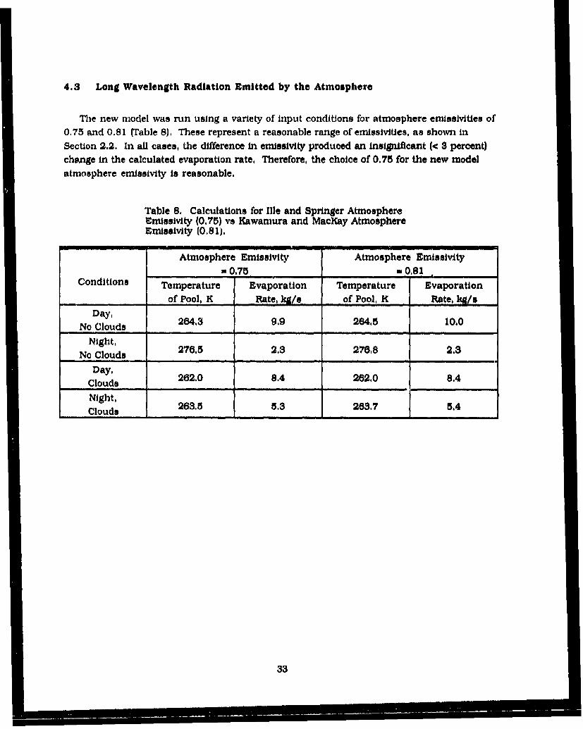
The new model was run using a variety of input conditions for atmosphere emissivities of0.75 and 0.81 (Table 8), These represent a reasonable range of emissivities, as shown inSection 2.2. In all cases, the difference in emnissivity produced an Insignificant (<' 3 percent)change in the calculated evaporation rate. Therefore, the choice of 0.75 for the new modelatmosphere emissivity is reasonable.

Table 8. Calculations for Ille and Springer AtmosphereEnmssivity (0.75) vs Kawamura and MacKay AtmosphereEmissivity (0,81).

Atmosphere Emissivity Atmosphere Emissivity

C t0.75 0,81Conditions Temperature Evaporation Temperature Evaporation

_..... ... _ of Pool, K Rate, kg/s of Pool, K Rate, kg/sDay,

No Clouds 264,3 9.9 264,5 10.0Night,

No Clouds 276,5 2.3 276,8 2,3Day, 262.0 8.4 262.0 8.4

Clouds ________

Clouds 263.5 5.3 263,7 5.4

33

4,4 Long Wavelength Radiation Emitted by the Pool

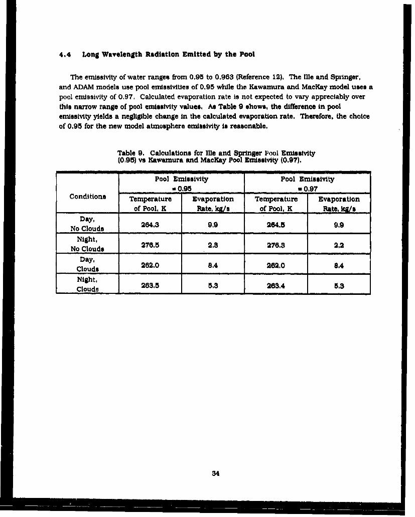
The emissivity of water ranges from 0.95 to 0.963 (Reference 12). The Ille and Splinger,and ADAM models use pool emnissivities of 0.95 while the Kawamura and MacKay model uses apool emissivity of 0.97, Calculated evaporation rate is not expected to vary appreciably overthis narrow range of pool emissivity values. As Table 9 shows, the difference in poolemissivity yields a negligible change in the calculated evaporation rate. Therefore, the choiceof 0.95 for the new model atmosphere emissivity is reasonable,

Table 9. Calculations for Mlle and Springer Pool Emissivity(0,95) vs Kawamura and MacKay Pool Emissivity (0,97).

Pool Emissivity Pool Emissivity=0.95 * 0,97

Conditions Temperature Evaporation Temperature Evaporation

_ .. ..__ of Pool, K Rate, kg/s of Pool, K Rate, kg/sDay, 264.3 9.9 264.5 9,9

N o C lou d s .... ....... .... .... ... ... .... .

Night,No Clouds 276,5 2.3 276.3 2.2

Day,Clouds 282.0 8.4 282,0 8,4Night,Clouds 263,5 5.3 263,4 5,3

34

4.5 Heat Conducted from the Ground

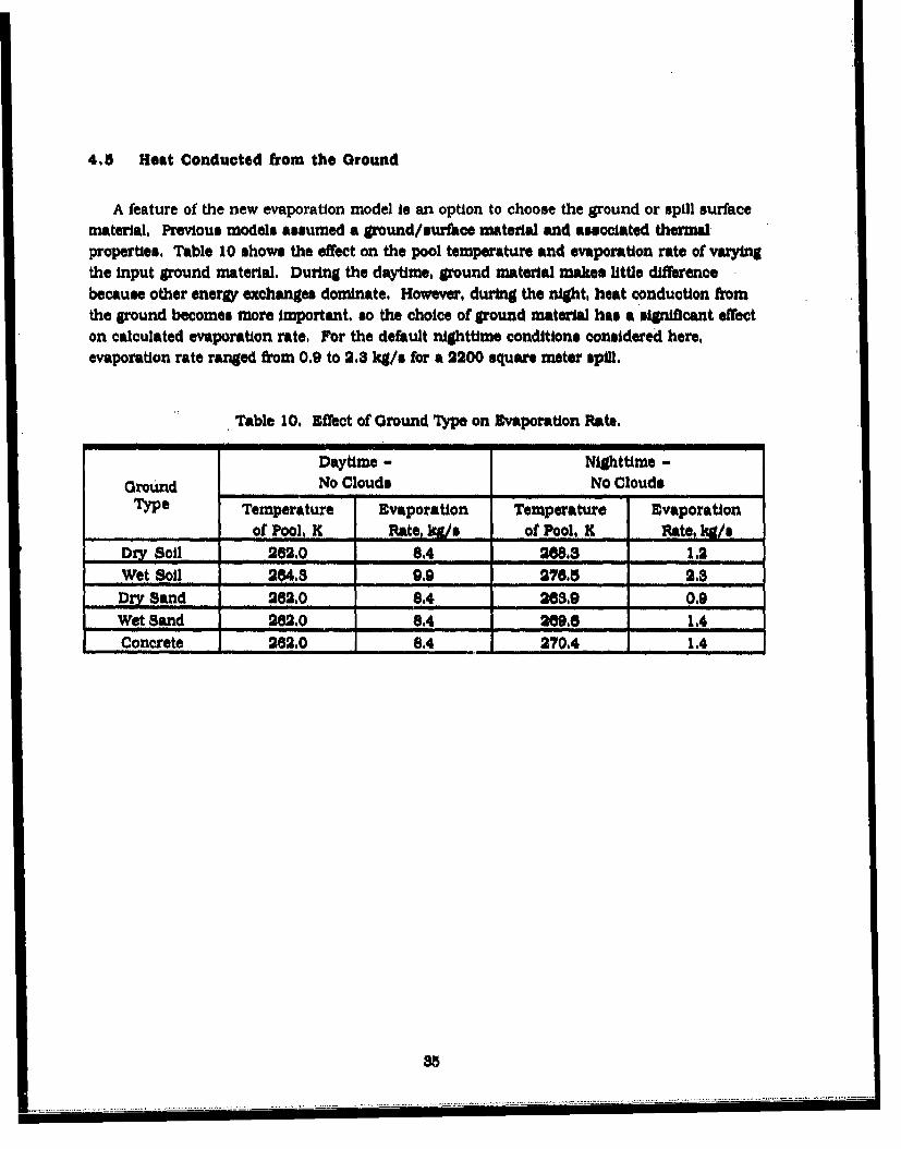
A feature of the new evaporation model is an option to choose the ground or spill surfacematerial, Previous models assumed a ground/surface material and associated thermalproperties. Table 10 shows the effect on the pool temperature and evaporation rate of varyingthe input ground material. During the daytime, ground material makes little differecebecause other energy exchanges dominate. However, during the night, heat conduction fromthe ground becomes more important, so the choice of ground material has a signiflcant effecton calculated evaporation rate, For the default nighttime conditions considered here,evaporation rate ranged from 0.9 to 2.3 kg/s for a 2200 square meter spill.

Table 10. Effect of Ground Type on Evaporation Rate.

Daytime - Nighttime -

Ground No Clouds No CloudsType Temperature Evaporation Temperature Evaporation

of Pool, K Rate,%/$ of Pool, K PAW, ADry Soil 282.0 8.4 288.3 1.2Wet Soil 264.3 9.9 278.5 2,.Dry Sand 262.0 8,4 263.9 0.9Wet Sand 282.0 0.4 269.8 1.4Concrete 262.0 8.4 270.4 1.4

- - .............

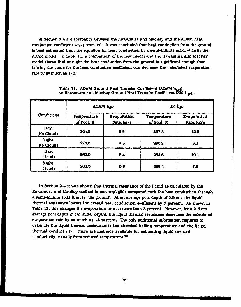
In Section 2.4 a discrepancy between the Kawamura and MacKay and the ADAM heatconduction coefficient was presented. It was concluded that heat conduction from the groundis best estimated from the equation for heat conduction in a seml-infinite solid,18 as in theADAM model. In Table 11, a comparison of the new model and the Kawamura and MacKaymodel show. that at night the heat conduction from the ground is significant enough thathalving the value for the heat conduction coefficient can decrease the calculated evaporationrate by as much as 1/3.

Table 11. ADAM Ground Heat Transfer Coefficient (ADAM h 4)vs Kawamura and MacKay Ground Heat Transfer Coefficient KMh),

ADAM hgrd KM hgrd

Conditions Temperature Evaporation Temperature Evaporation

of Pool, K Rate, kg/s of Pool, K Rate, kg/sDay,

No Clouds 264.3 9,9 267.5 12,5

Night,No Clouds 276,5 2.3 280,2 3.0

Day,Clouds 262.0 8,4 264.6 10.1Night,Niuds 263,5 5.3 268.4 7.5, Qlouds .....

In Section 2.4 it was shown that thermal resistance of the liquid as calculated by theKawamura and MacKay method is non-negligible compared with the heat conduction throughR seml-i-fnite solid (that is, the ground). At an average pool depth of 0,5 cm, the liquidthermal resistance lowers the overall heat conduction coefficient by 7 percent. As shown inTable 12, this changes the evaporation rate no more than 3 percent. However, for a 2.5 cmaverage pool depth (5 cm initial depth), the liquid thermal resistance decreases the calculatedevaporation rate by as much as 14 percent, The only additional information required tocalculate the liquid thermal resistance is the chemical boiling temperature and the liquidthermal conductivity, There are methods available for estimating liquid thermalconductivity, usually from reduced temperature.2 4

36

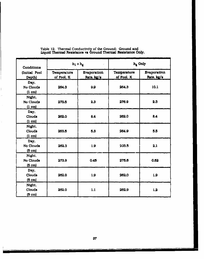
Table 12. Thermal Conductivity of the Ground: Ground andLiquid Thermal Resistance vs oround Thermal Resistance Only.

Conditions h, +h9 hg Only

(Initial Pool Temperature Evaporation Temperature EvaporationDepth) of Pool, K Rate, g/s i of Pool, K Rate, kg/s

Day,No Clouds 264.3 9.9 264.3 10.1

(1 era)__ _ _ _ __ _ _ _ __ _ _ _ __ _ _ _

Night,No Clouds 276.5 2.3 276.9 2.3

(I cm ) .... .. ... ...

Day,Clouds 262.0 8.4 262.0 8,4

Night,Clouds 263,5 5.3 264.9 5.5

(I ( Icm ) .... . ..

Day,No Clouds 262.3 1,9 233.5 2.1

(5 cm ) .. . ..... ..

Night,No Clouds 273.9 0.45 275.6 0.52

(5 cm)

Day,Clouds 262.0 1.9 262.0 1.9(5 cm ) .......... ......

Night,Clouds 262.0 1.1 262,9 1.2(5 cm)

37

4,6 Heat Lose Due to Evaporation

4,6.1 PROPERTIES OF VAPOR ABOVE POOL

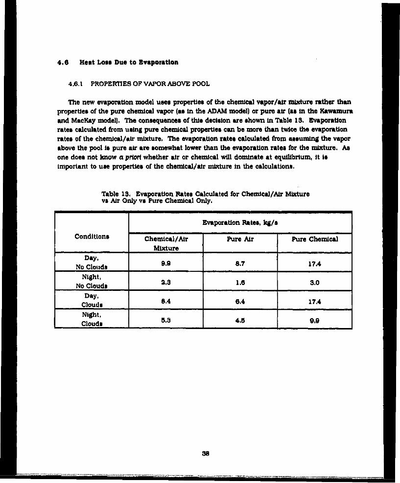
The new evaporation model uses properties of the chemical vapor/air mixture rather thanproperties of the pure chemical vapor (as in the ADAM model) or pure air (as in the Kawamuraand MacKay model). The consequences of this decision are shown in Table 13, Evaporationrates calculated from using pure chemical properties can be more than twice the evaporationrates of the chemical/air mixture. The evaporation rates calculated from assuming the vaporabove the pool is pure air are somewhat lower than the evaporation rates for the mixture. Asone does not know a prior( whether air or chemical will dominate at equilibrium, it isimportant to use properties of the chemical/air mixture in the calculations,

Table 13. Evaporation Rates Calculated for Chemical/Air Mixturevs Air Only vs Pure Chemical Only.

Evaporation Rates, kg/s

Conditions Chemical/Air Pure Air Pure Chemical

Mixture

Day,No Clouds 8,7 17.4

Night,No Clouds

Day,Clouds 8.4 6.4 17,4Night,Clouds 1,3 4,5_9,9

38

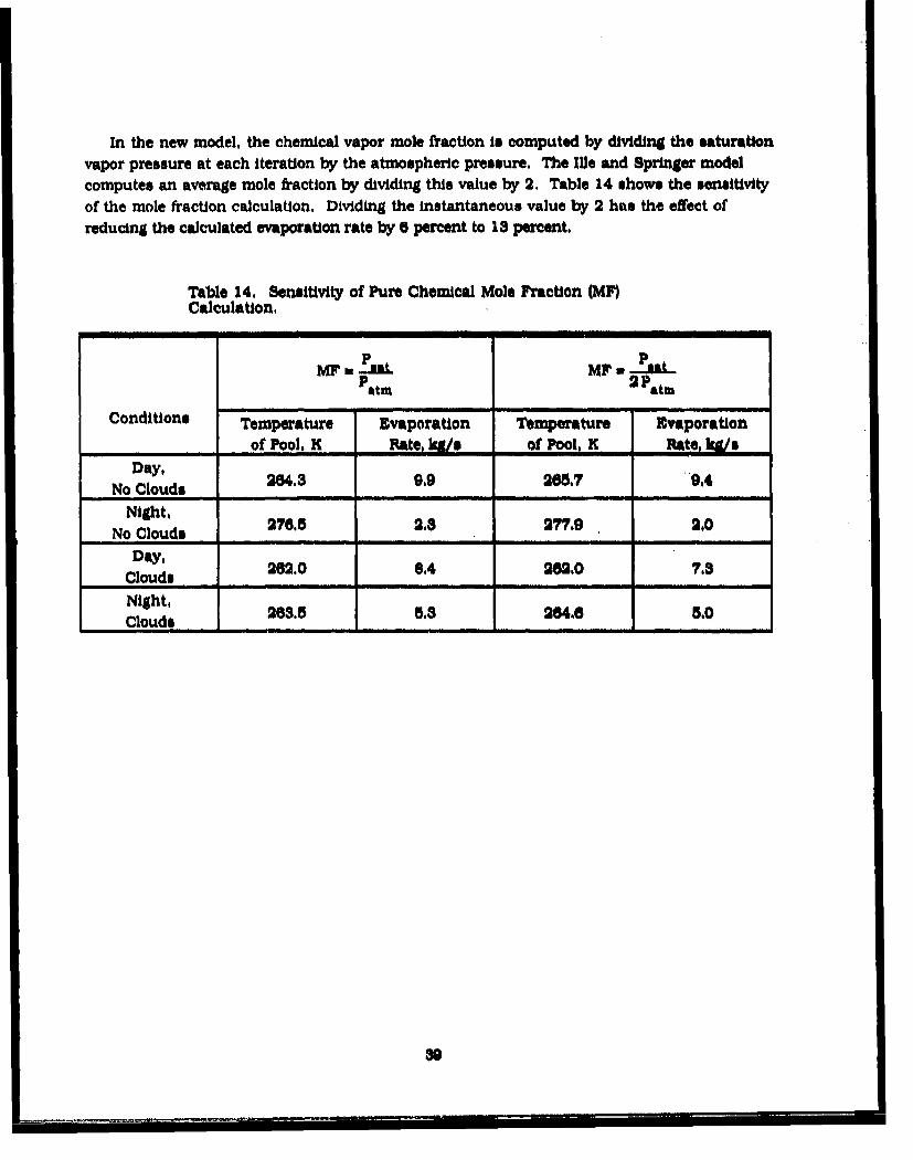
In the new model, the chemical vapor mole fraction is computed by dividing the saturationvapor pressure at each iteration by the atmospheric pressure. The Ille and Springer modelcomputes an average mole fraction by dividing this value by 2. Table 14 shows the sensitivityof the mole fraction calculation. Dividing the instantaneous value by 2 has the effect ofreducing the calculated evaporation rate by 5 percent to 13 percent,

Table 14. Sensitivity of Pure Chemical Mole Fraction (MF)Calculation.

P pMF LmLL MP--atPatm 2 Pat,-

Conditions Temperature Evaporation Temperature Evaporation

_. .. ..... of Pool, K t /s of Pool, K Rate, We/s

Day,No Clouds 2*4.3 9.9 265.7 9,4

Night,No Clouds 276.5 2,3 277.9 2.0

Day,Clu, 262.0 8.4 262.0 7,8CloudsNight,Clouds 263.5 5.3 264.6 5.0Clouds.

39

4.6.2 MASS TRANSFER COEFFICIP.Nr

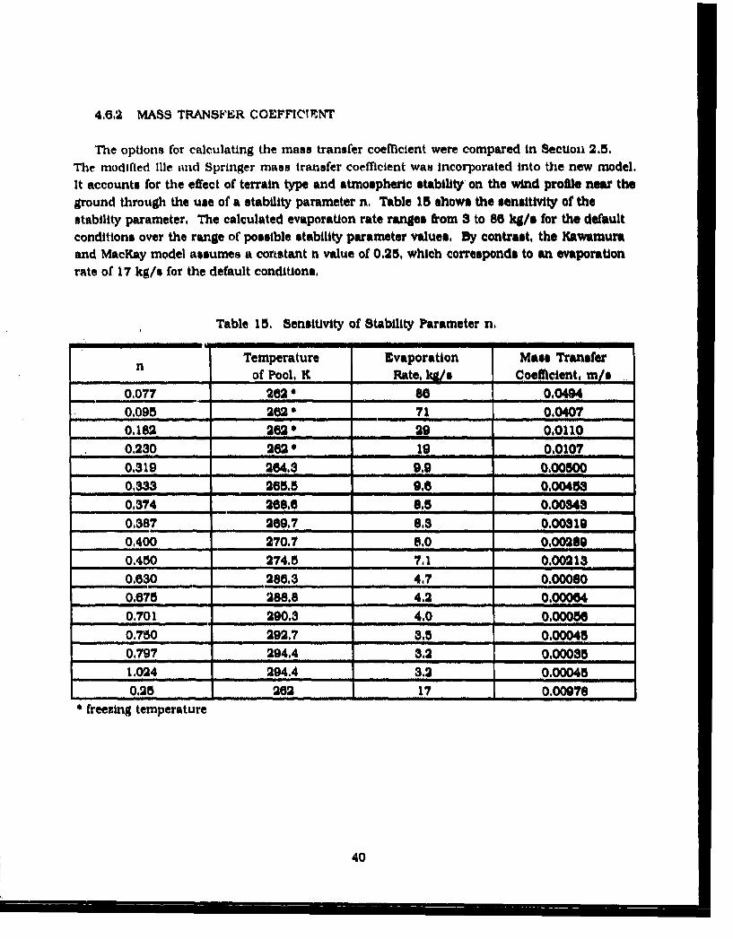
The options for calculating the mass transfer coefficient were compared in Section 2.5,The modified ille and Springer mass transfer coefficient was incorporated into the new model.It accounts for the effect of terrain type and atmospheric stability on the wind profile near theground through the use of a stability parameter n. Table 15 shows the sensitivity of thestability parameter. The calculated evaporation rate ranges from 3 to 86 kg/s for the defaultconditions over the range of possible stability parameter values, By contrast, the Kawamuraand MacKay model assumes a constant n value of 0.25, which corresponds to an evaporationrate of 17 kg/s for the default conditions,

Table 15, Sensitivity of Stability Parameter n,

n Temperature Evaporation Mass TransferSof Pool, K Rate, kg/s Coefficient, m/s

0.077 262 86 0.04940.095 262 * 71 0.04070.182 262, 29 0.0110

0.230 262* 1i 090107

0.319 264.3 9,9 0.00500

0.333 265.5 9.6 0.00453

0.374 268.66 0,._ 0.0034_

0,387 269.7 8,3 0,00319

0,400 270.7 8,0 0.002890.450 274J5 7.1 0.002130.630 28G.3 4,7 0.00060

0.675 288.8 4.2 0.000640.701 290.3 4.0 0,000560.750 292,7 3.5 0,00045

0,797 294.4 3.2 0.00035

1.024 294.4 3.2 0.00045

0.25 262 17 0.00976* freezing temperature

40

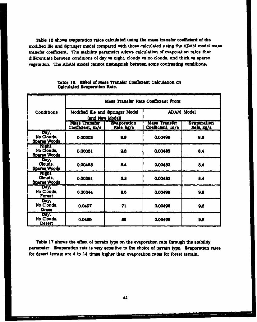
Table 16 shows evaporation rates calculated using the mass transder coeficient of themodified Jie and Springer model compared with those calculated using the ADAM model masstransfer coefficient, The stability parameter allows calculation of evaporation rates thatdifferentlate between conditions of day vs night, cloudy vs no clouds, and thick ve sparse

vegetation. The ADAM model cannot distinguish between some contrasting conditions.

Table 16. ffftt of Mass Transfer Coefficient Calculation onCalculated Evaporation Rate,

Mass Trmnsir Rate Coefficient from:

Conditions Modified Mel and Springer Model ADAM Model"s gd Model)__ ___

Mass Trane vaporaton as Transfer Ivaporation,, Coefflcient, m/s Zre!, we Coecftent, m/s ae /

Day,NO Clouds, 0.00602 9,9 0,00498 9,8S1parse Iod

wlig t , l| II I I I I I I

No Clouds, 0,00051 2,8 0,00408 8,4Aparse Woods

Clouds, 0.00488 8,4 0.004S8 8.4Spase Woods ....... _ _ __ _ _ _ __ _ _ _ _ __ _ _

Clouds, 0.002,8 5,3 0.00483 ,4Sparse Woods...DAY#

No Clouds, 0.00344 a,' 0.00498 9.8ForestDay,

No Clouds, 0,0407 71 0.00498 9.0Oras* ...... ..Day,

No Clouds, 0.0495 a6 0,004o 8 9,8Desert .. .. ... ..

Table 1? shows the effect of terrain type on the evaporation rate through the stabilityparameter. Evaporation rate is very sensitive to the choice of terrain type, Evaporation ratesfor desert terrain are 4 to 14 times higher than evaporation rates for forest terrain.

41

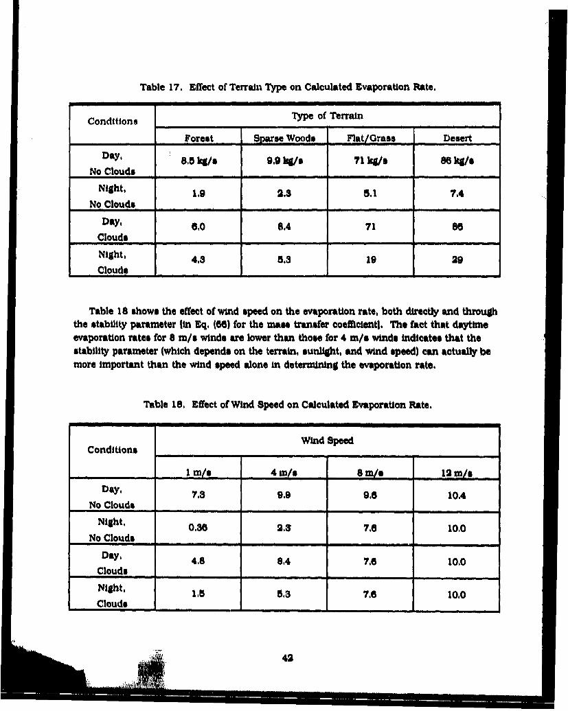
Table 17. Effect of Terrain Type on Calculated Evaporation Rate,

Conditions Type of Terrain

_ Forest Sparse Woods Flat/Grass Desert

Day, 8,5 kg/s 9,9 kg/s 71 kg/s Be kg/sNo Clouds -_I

Night, 1,9 2.3 5.1 7,4

No Clouds

Day, 6,0 8,4 71 86

Clouds

Night, 4.3 5.3 19 29

Clouds........ .. I

Table 18 shows the effect of wind speed on the evaporation rate, both directly and throughthe stability parameter [in Eq, (66) for the mass transfer coefficientl. The fact that daytimeevaporation rates for 8 m/s winds are lower than those for 4 m/s winds indicates that thestability parameter (which depends on the terrain, sunlight, and wind speed) can actually bemore important than the wind speed alone in determining the evaporation rate.

Table 18, Effect of Wind Speed on Calculated Evaporation Rate.

Wind SpeedConditions .... .. ... ... .. .___ ____ _.. ... ... ..___ __i

/I ms 4 wrs 8wm/G 12 m/0Day, 7.3 9 .9 9 .6 10 .4

No Clouds

Night, 0.36 2.3 7,6 10.0

No Clouds

Day, 4.8 8.4 7,6 10.0

Clouds

Night, 1.5 5.3 7.6 10,0

Clouds _ . . . .. .

42

l .. . .. .

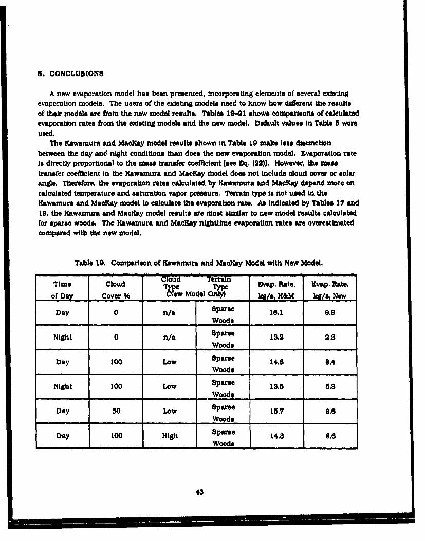
8. CONCLUSIONS

A new evaporation model has been presented, incorporating elements of several existingevaporation models, The users of the existing models need to know how different the resultsof their models are from the new model results. Tables 19-21 shows comparisons of calculatedevaporation rates from the existing models and the new model, Detfult values in Table 5 wereused,

The Kawamura and MacKay model results shown in Table 19 make less distinctionbetween the day and night conditions than does the new evaporation model, Evaporatlon rateis directly proportional to the mass transfer coefficient [see Sq. (22)}, However, the masstransfer coefficient in the Kawamura and MacKay model does not include cloud cover or solarangle. Therefore, the evaporation rates calculated by Kawamura and MacKay depend more oncalculated temperature and saturation vapor pressure. Terrain type is not used in theKawamura and MacKay model to calculate the evaporation rate, As indicated by Tables 17 and19, the Kawamura and MacKay model results are most similar to new model results calculatedfor sparse woods, The Kawamura and MacKay nighttime evaporation rates are overestimatedcompared with the new model,

Table 19, Comparison of Kawamura and MacKay Model with New Model.

Time Cloud cloudTerran vap, Rate, avap, Rate,of Day Cover % (New Model 01*)y kg/t,K&M kg/s, New

Day 0 n/a Sparse 16.1 9,9Woods

Night 0 n/a Sparse 13,2 2,3Woods

Day 100 Low Sparse 14.3 8.4Woods

Night 100 Low Sparse 13.5 5.3Woods

Day 50 Low Sparse 15.7 9.6Woods

Day 100 High Sparse 14,3 8.6Woods

43

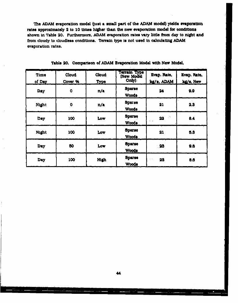
The ADAM evaporation model Quet a small part of the ADAM model) yields evaporationrate. approximately 2 to 10 times higher than the new evaporation model for conditionsshown in Table 20. rurthermore, ADAM evaporation rates vary little from day to night andfrom cloudy to cloudless conditions. Terrain type is not used in calculating ADAMevaporation rates,

Table 20, Comparison of ADAM Evaporation Model with New Model,

Time Cloud Cloud (New. Model 'vap. Rate, Evap. Rate,

of Day Cover % Type only) U/e, ADAM X ., Now

Day 0 n/a Sp2re 24 9.9Woods _

Night 0 n/a Sparse 21 2.3Woods _ _ _

Day 100 LOWPaU 22 8.4Woods "_ _

Night 100 Low Sparse 21 5.$Woods

Day s0 Low a2se 28 9,6Woods

Day 100 High Sparse 28 8.6Woods

44

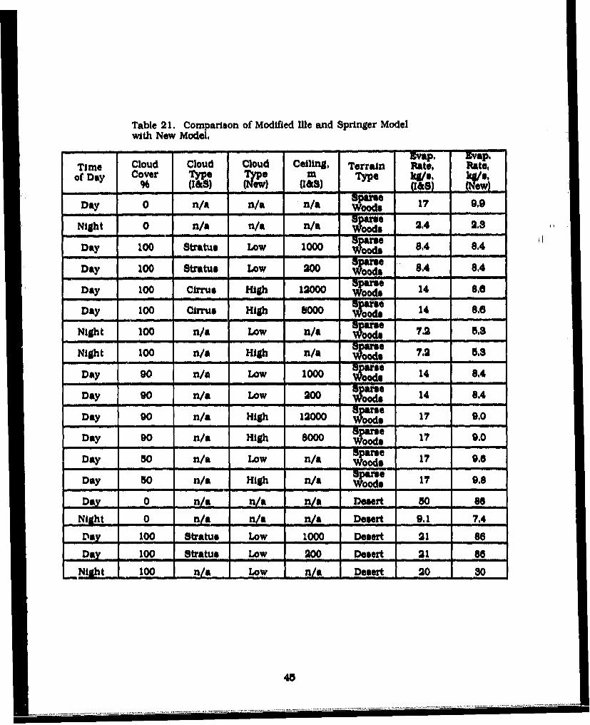
Table 21. Comparison of Modified Ille and Springer Modelwith New Model,

- -loud u Cvap, vap.Time Cloud Cloud Cloud Ceiling, Terrain Rate, Rate,

ofDa Cover Type Type M Tp gs gs96~s 03)s 06 ,d•,' ... ... Sparse

Day 0 n/a n/a n/a Woods 17 9.9

Night 0 n/a n/a n/a sparse 2.4 2,3- oods�. 8.4 .4

Day 100 Stratum Low 200 8.4 8.4---

Day 100 Cirrus High 12000 sm 14 8.6

Day 100 Cirrus High 8000 s 14 8.6

Night 100 n/a Low n/a 7.2 5.8

Night 100 n/a High n/a some 7.2 5,.

Day 90 n/a Low 1000 sprs 14 8.4Woods

Day 90 n/a Low 200 Sparse 14 .4

Day 90 n/a High 12000 spars 17 9.0SSparse

Day 90 n/a High 8000 Woods 17 9.0

Day 50 n/a Low n/a s e 17 9.6

Day SO n/a High n/a 1ors 17 9.,

0Day 0 n/a n/a n/a Desert 50 6

Night 0 n/a n/a n/a Desert 9.1 7,4

Da 100 Stratus Low 1000 Desert 21 B6

,ay 100 Stratum Low 200 Desert 21 86LNight 100 n/a -Lowna eet 0

-/DLswrt 20-

45

Comparisons of the new model with the llle and Springer model are shown in Table 21.The new evaporation model is most similar to the modified Ille and Springer model, Theseare the only evaporation models presented which use the stability parameter to estimate theeffect of the wind profile. A drawback of the modified Ille and Springer model is that whencloud cover is less than 100 percent and the ceiling is greater than 4878 m, or when the cloudcover is S 50 percent, the model calculates the same evaporation rate as for no cloud cover,The modified Ile and Springer model does not consider cloud type when cloud cover is lessthan 100 percent, but it does allow selection of a ceiling height, which is related to cloud type.It also considers terrain type, as indicated by the difference between sparse woods and desertterrain, The modified Tlle and Springer model yields higher evaporation rates than the newmodel for the sparse woods terrain. It yields mostly lower evaporation rates than the newmodel for desert terrain. In general, the new model yields a greater distinction between cloudconditions and terrain types,

The new evaporation model presented in this report is a composite of existing steady stateevaporation models, and is an Improvement upon existing models, The model is simpleenough to run on a PC, but is complex enough to require a substantial amount of chemicaldata,

To put the model results into perspective, it is worth noting some of its shortcomings, Thenew model assumes that the spill surface is flat and impermeable. That is unlikely to be thecase, unless the spill surface is concrete, The spill is assumed to be instantaneous, which isnot always true, The spill surface area is assumed to be constant, and an average uniformdepth is assumed, Again, these are unlikely to hold true in a real spill. In calculating the heatdue to solar radiation, a constant pool albedo is assumed, In reality, the albedo of the poolwill vary with solar angle, In a spill area with dense vegetation, buildings, or other structures,the pool may be shielded from direct sunlight, even on a cloudless day, Furthermore, seasonwill determine the sparseness of the vegetation, This affects both terrain roughness and solarradiation reaching the pool, The stability parameters used in calculating the mass transfercoefficient are from a single reference source, and apply only to rural areas, An independentverification of these data would place greater confidence in them,

The new model does not consider temperature changes once the temperature is greater thanthe boiling point or less than the freezing point. It Is unlikely that the liquid chemicaltemperature will exceed the boiling point at ambient pressures. However, the temperaturecould continue to decrease once the pool has frozen. A number of factors are affected if thechemical freezes and falls below the freezing point. The heat of sublimation (rather than theheat of vaporization) would be required to calculate the evaporation rate. The ground thermalproperties may change if the ground is also frozen, The thermal resistance of the pool itselfwill change when it becomes a solid. Both of these affect the heat conducted from the ground,The albedo of a frozen pool Is much higher than that of a liquid pool, so the amount of directsolar heating would be less than for a liquid. The vapor pressure equation is generally notvalid for a solid. A temperature-vapor pressure relationship for the solid chemical would berequired.

46

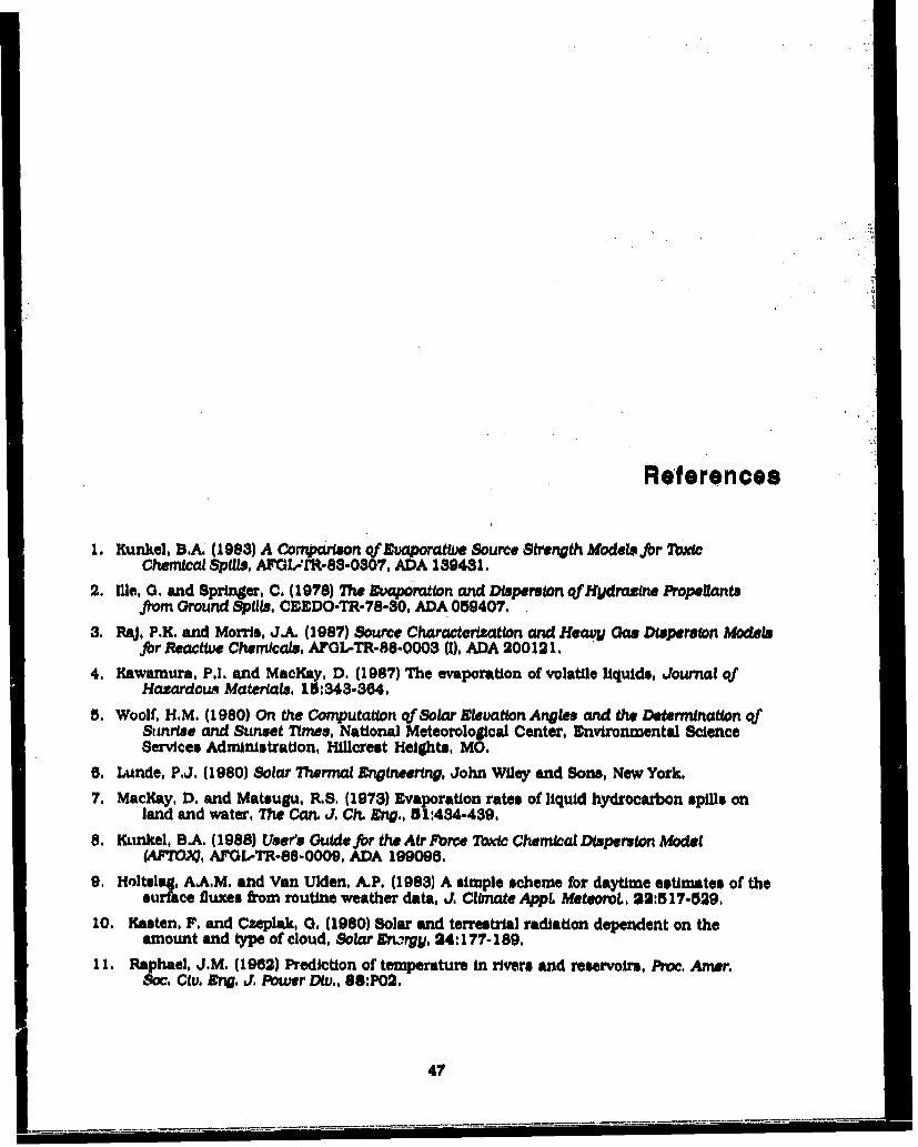
Ref erences

1. Kunkel, B.A. (1983) A Comparison QfEvaporatwe Source St•ngth Model, for TbidcChemical Spills, AFOL-RM-88-0307, ADA 139481.

2. Ille, 0. and Springer, C. (1978) The Evaporation and Dispersion QfHydrazine Propellantsfiom Ground Spills, CEEDO-TR-78-30, ADA 059407.

3. Raj. P.K. and Morris, J.A. (1987) Source Characterization and Heavy G~as Dispersion Modelsfor Reactive Chemicals, AFOL-TR-88-0003 (I), ADA 200121.

4, Kawamura, P.I. and MacKay, D. (1987) The evaporation of volatile liquids, Journal QfHazardous Materials, 10:343-364,

5. Woolf, H.M, (1980) On the Computation of Solar Elevation Angles and the Determination ofSunrise and Sunset Times, National Meteorological Center, Environmental ScienceServices Adminlstration, Hillcrest Heights, MO.

6. Lunde, P.J, (1980) Solar Thermal Engineering, John Wiley and Sons, New York.

7. MacKay, D, and Matsugu, R.S, (1973) Evaporation rates of liquid hydrocarbon spills onland and water, The Canm J, Ch. Eng.. 81:434-439.

8. Kunkel, B.A. (1988) User's Guide for the Air Force Tbxic Chemical Dispersion Model(AFOPTOO, AFGL-TR-88-0009, ADA 199096.

9, Holtelas, AA,M. and Van Ulden, A.P. (1983) A simple scheme for daytime estimates of thesurface fluxes from routine weather data, J. Climate AppL MeteoroL, 22:517-529,

10. Masten, F, and Czeplak, 0, (1980) Solar and terrestrial radiation dependent on theamount and type of cloud, Solar Enorgy, 24:177-189,

11. Raphael, J.M. (1962) Prediction of temperature in rivers and reservoirs, Proc, Amer.Smo. Clv. Eg. J. Power Div., 86:P02.

47

12. McAdams, W.H. (1954) Heat Transmission, 3rd edn., McGraw-Hill Book Company, Inc,,New York.

13. Holman, J.P. (1976) Heat Transfer, 4th edn., McGraw-Hill Book Company, Inc,, New York.

1.4, Bird, R.B., Stewart, W,E,, and Lightfoot, E,N, (1960) Transport Phenomena, John Wiley andSona, Inc., New York,

15, Schneider, P,J. (1955) Conduction Heat Transfer, Addison-Wesley Publishing Co.,Cambridge, MA.

16, Dean, J.A, (1985) ed. Lange's Handbook qf Chemistry, 13th edn., McGraw-Hill BookCompany, New York.

17, Kothandaraman, CP. and Subramanyan, S. (1975) Heat and Mass T"anhfer Data Book,2nd edn., John Wiley and Sons, New York.

18. Sutton, 0.0, (1958) Micrometeorology, McGraw-Hill Book Company, Inc., New York,

19. Smedman-Hogstrom, A.S. and Hogatrom, U. (1978) A practical method for determiningwind frequency distribution for the lowest 200 m from routine meteorological data, J.QfAppl. MeteoroL, 17:942-954,

20. Fuller, E.N. and Giddings, J.C. (1965) A comparison of methods for predicting gaseousdiffusion coefficients, J,, Gas Chromatogr,, 8:222-227.

21. Fuller, E.N., Ensley, KX, and Giddings, J.C, (1969) Diffusion of halogenated hydrocarbonsin helium: The effect of structure on collision cross sections, J. Phys, Chem. 78:8679.3685.

22. Fuller, EXN, Schlettler, P.D., and Giddings, J.0, (1966) A new method for prediction ofbinary gas-phase diffusion coefficients, nd. EMV. Chem, 56: 18-27.

23, Perry, RH., and Chilton, CH,, eds, (1973) Chemical Engineers' Handbook, 5th edn,,McGraw-Hill Book Company, Inc., New York,

24, Reid, R.C,, Prausnltz, J,M,, and Poling, BE,, (1987) The Properties of Gases and Liquids, 4thedn,, McGraw-Hill Book Company, Inc., New York.

25. Schmidt, EW. (1984) Hydrasine and Its Derivatives: Preparation, Propertin, andApplications, John Wiley and Sons, New York,

U. 9, UOV[YC MMRN T I'[ITlltNU nPPIMl,9 1020--700-0U00/20007

48