Chemical Equilibrium. Copyright © Houghton Mifflin Company.All rights reserved. Presentation of Lecture Outlines, 15–2 Chemical Equilibrium When compounds

Chemical Equilibrium

Copyright © Houghton Mifflin Company.All rights reserved. Presentation of Lecture Outlines, 15–2


• When compounds react, they eventually form a mixture of products and unreacted reactants, in a dynamic equilibrium.

– A dynamic equilibrium consists of a forward reaction, in which substances react to give products, and a reverse reaction, in which products react to give the original reactants.

– Chemical equilibrium is the state reached by a reaction mixture when the rates of the forward and reverse reactions have become equal.



– Much like water in a U-shaped tube, there is constant mixing back and forth through the lower portion of the tube.

– It’s as if the forward and reverse “reactions” were occurring at the same rate.

– The system appears to static (stationary) when, in reality, it is dynamic (in constant motion). (see Figure 15.3)

“reactants” “products”



• For example, the Haber process for producing ammonia from N2 and H2 does not go to completion.

– It establishes an equilibrium state where all three species are present.

(g)2NH )g(H3)g(N 322


A Problem to Consider

• Applying Stoichiometry to an Equilibrium Mixture.

– What is the composition of the equilibrium mixture if it contains 0.080 mol NH3?

– Suppose we place 1.000 mol N2 and 3.000 mol H2 in a reaction vessel at 450 oC and 10.0 atmospheres of pressure. The reaction is

(g)2NH )g(H3)g(N 322



– The equilibrium amount of NH3 was given as 0.080 mol. Therefore, 2x = 0.080 mol NH3 (x = 0.040 mol).

• Using the information given, set up the following table.

(g)2NH )g(H3 )g(N 322

Starting 1.000 3.000 0Change -x -3x +2x

Equilibrium1.000 - x 3.000 - 3x 2x = 0.080 mol



• Using the information given, set up the following table.

Equilibrium amount of N2 = 1.000 - 0.040 = 0.960 mol N2

Equilibrium amount of H2 = 3.000 - (3 x 0.040) = 2.880 mol H2

Equilibrium amount of NH3 = 2x = 0.080 mol NH3

(g)2NH )g(H3 )g(N 322

Starting 1.000 3.000 0Change -x -3x +2x

Equilibrium1.000 - x 3.000 - 3x 2x = 0.080 mol


The Equilibrium Constant

• Every reversible system has its own “position of equilibrium” under any given set of conditions.

– The ratio of products produced to unreacted reactants for any given reversible reaction remains constant under constant conditions of pressure and temperature.

– The numerical value of this ratio is called the equilibrium constant for the given reaction.



• The equilibrium-constant expression for a reaction is obtained by multiplying the concentrations of products, dividing by the concentrations of reactants, and raising each concentration to a power equal to its coefficient in the balanced chemical equation.

ba

dc

c ]B[]A[

]D[]C[K

– For the general equation above, the equilibrium-constant expression would be:

dDcC bBaA



• The equilibrium-constant expression for a reaction is obtained by multiplying the concentrations of products, dividing by the concentrations of reactants, and raising each concentration to a power equal to its coefficient in the balanced chemical equation.

ba

dc

c ]B[]A[

]D[]C[K

– The molar concentration of a substance is denoted by writing its formula in square brackets.

dDcC bBaA



• The equilibrium constant, Kc, is the value obtained for the equilibrium-constant expression when equilibrium concentrations are substituted.– A large Kc indicates large concentrations of products

at equilibrium.

– A small Kc indicates large concentrations of unreacted reactants at equilibrium.



• The law of mass action states that the value of the equilibrium constant expression Kc is constant for a particular reaction at a given temperature, whatever equilibrium concentrations are substituted.

– Consider the equilibrium established in the Haber process.

(g)2NH )g(H3)g(N 322



• The equilibrium-constant expression would be

– Note that the stoichiometric coefficients in the balanced equation have become the powers to which the concentrations are raised.

(g)2NH )g(H3)g(N 322

322

23

c ]H][N[

]NH[K


Equilibrium: A Kinetics Argument

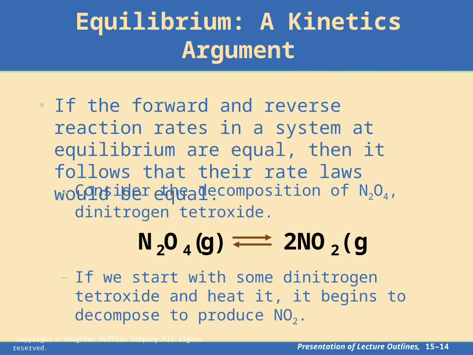
• If the forward and reverse reaction rates in a system at equilibrium are equal, then it follows that their rate laws would be equal.

– If we start with some dinitrogen tetroxide and heat it, it begins to decompose to produce NO2.

– Consider the decomposition of N2O4, dinitrogen tetroxide.

(g)2NO )g(ON 242



• If the forward and reverse reaction rates in a system at equilibrium are equal, then it follows that their rate laws would be equal.

– Consider the decomposition of N2O4, dinitrogen tetroxide.

– However, once some NO2 is produced it can recombine to form N2O4.

(See Animation: Equilibrium Decomposition of N2O4)

(g)2NO )g(ON 242



– Call the decomposition of N2O4 the forward reaction and the formation of N2O4 the reverse reaction.

(g)2NO )g(ON 242

kf

kr

– These are elementary reactions, and you can immediately write the rate law for each.

]ON[kRate 42f(forward) 2

2r(reverse) ]NO[kRate

Here kf and kr represent the forward and reverse rate constants.



– Ultimately, this reaction reaches an equilibrium state where the rates of the forward and reverse reactions are equal. Therefore,

(g)2NO )g(ON 242

22r42f ]NO[k]ON[k

kf

kr



– Combining the constants you can identify the equilibrium constant, Kc, as the ratio of the forward and reverse rate constants.

(g)2NO )g(ON 242

]ON[]NO[

kk

K42

22

r

fc

kf

kr


Obtaining Equilibrium Constants for Reactions

• Equilibrium concentrations for a reaction must be obtained experimentally and then substituted into the equilibrium-constant expression in order to calculate Kc.



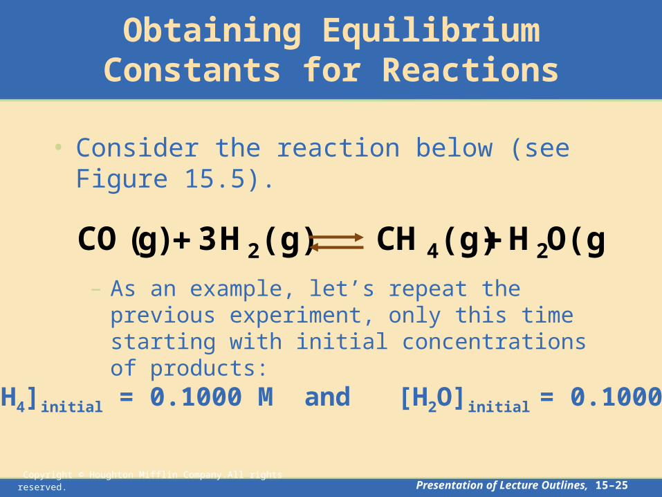
• Consider the reaction below (see Figure 15.5).

O(g)H (g)CH (g)H 3 )g(CO 242

– Suppose we started with initial concentrations of CO and H2 of 0.100 M and 0.300 M, respectively.


– When the system finally settled into equilibrium we determined the equilibrium concentrations to be as follows.

Reactants Products[CO] = 0.0613 M[H2] = 0.1893 M

[CH4] = 0.0387 M[H2O] = 0.0387 M



O(g)H (g)CH (g)H 3 )g(CO 242


– The equilibrium-constant expression for this reaction is:

32

24c ]H][CO[

]OH][CH[K



O(g)H (g)CH (g)H 3 )g(CO 242


– If we substitute the equilibrium concentrations, we obtain:

93.3)M1839.0)(M0613.0(

)M0387.0)(M0387.0(K 3c



O(g)H (g)CH (g)H 3 )g(CO 242


– Regardless of the initial concentrations (whether they be reactants or products), the law of mass action dictates that the reaction will always settle into an equilibrium where the equilibrium-constant expression equals Kc.



O(g)H (g)CH (g)H 3 )g(CO 242


– As an example, let’s repeat the previous experiment, only this time starting with initial concentrations of products:

[CH4]initial = 0.1000 M and [H2O]initial = 0.1000 M



O(g)H (g)CH (g)H 3 )g(CO 242


– We find that these initial concentrations result in the following equilibrium concentrations.

Reactants Products

[CO] = 0.0613 M

[H2] = 0.1893 M

[CH4] = 0.0387 M

[H2O] = 0.0387 M



O(g)H (g)CH (g)H 3 )g(CO 242


– Substituting these values into the equilibrium-constant expression, we obtain the same result.

93.3)M1839.0)(M0613.0(

)M0387.0)(M0387.0(K 3c

– Whether we start with reactants or products, the system establishes the same ratio.



O(g)H (g)CH (g)H 3 )g(CO 242


The Equilibrium Constant, Kp

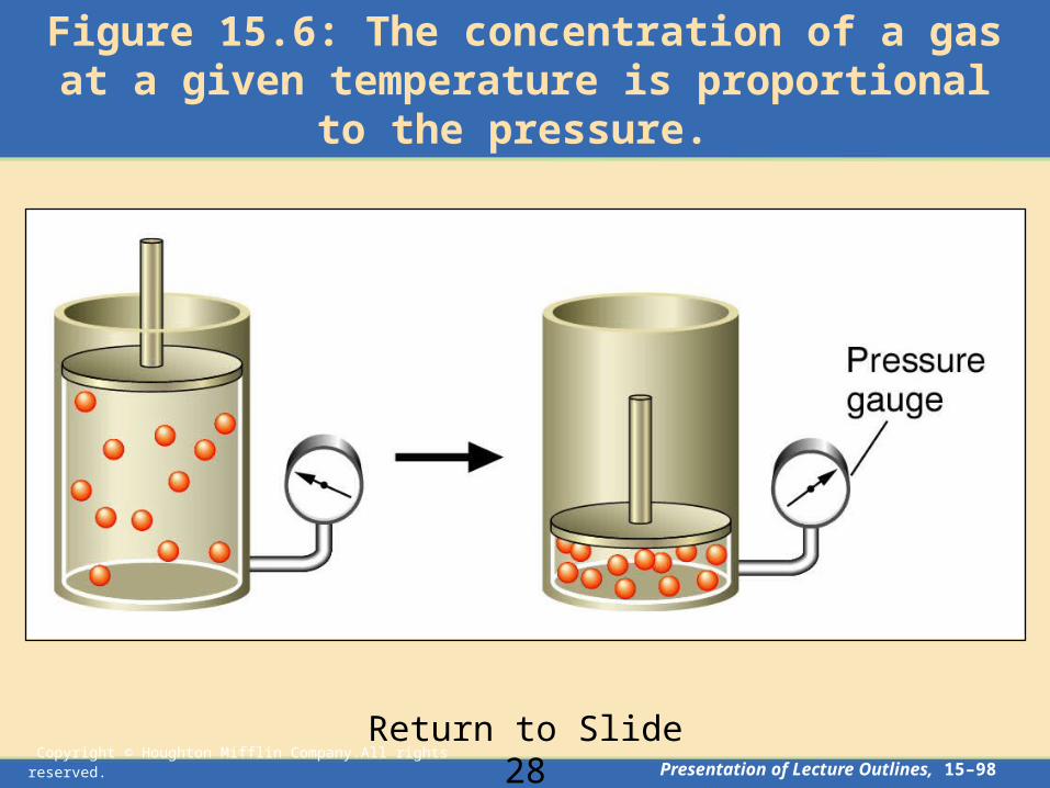
• In discussing gas-phase equilibria, it is often more convenient to express concentrations in terms of partial pressures rather than molarities (see Figure 15.6 and Animation: Pressure and Concentration of a Gas).

– It can be seen from the ideal gas equation that the partial pressure of a gas is proportional to its molarity.

MRTRTVn

P )(



• If we express a gas-phase equilibria in terms of partial pressures, we obtain Kp.

– Consider the reaction below.

O(g)H (g)CH (g)H 3 )g(CO 242 – The equilibrium-constant expression in terms of

partial pressures becomes:

3HCO

OHCHp

2

24

K

PP

PP



• In general, the numerical value of Kp differs from that of Kc.– From the relationship n/V=P/RT, we can show that

where n is the sum of the moles of gaseous products in a reaction minus the sum of the moles of gaseous reactants.

ncp )RT(KK



• Consider the reaction

– Kc for the reaction is 2.8 x 102 at 1000 oC. Calculate Kp for the reaction at this temperature.

(g)SO 2 )g(O)g(SO2 322



– We know thatn

cp )RT(KK

From the equation we see that Dn = -1. We can simply substitute the given reaction temperature and the value of R (0.08206 L.atm/mol.K) to obtain Kp.


(g)SO 2 )g(O)g(SO2 322



– Sincen

cp )RT(KK

3.4 K) 1000 08206.0( 108.2K 1-Kmol

atmL2p


(g)SO 2 )g(O)g(SO2 322


Equilibrium Constant for the Sum of Reactions

• Similar to the method of combining reactions that we saw using Hess’s law in Chapter 6, we can combine equilibrium reactions whose Kc values are known to obtain Kc for the overall reaction.– With Hess’s law, when we reversed reactions or

multiplied them prior to adding them together, we had to manipulate the H’s values to reflect what we had done.

– The rules are a bit different for manipulating Kc.


2. If you multiply each of the coefficients in an equation by the same factor (2, 3, …), raise Kc to the same power (2, 3, …).

3. If you divide each coefficient in an equation by the same factor (2, 3, …), take the corresponding root of Kc (i.e., square root, cube root, …).

4. When you finally combine (that is, add) the individual equations together, take the product of the equilibrium constants to obtain the overall Kc.

1. If you reverse a reaction, invert the value of Kc.



• For example, nitrogen and oxygen can combine to form either NO(g) or N2O (g) according to the following equilibria.

NO(g) 2 )g(O)g(N 22

O(g)N )g(O)g(N 2221

2

Kc = 4.1 x 10-31

Kc = 2.4 x 10-18

(1)

(2)

Kc = ?

– Using these two equations, we can obtain Kc for the formation of NO(g) from N2O(g):

NO(g) 2 )g(O)g(ON 221

2 (3)



• To combine equations (1) and (2) to obtain equation (3), we must first reverse equation (2). When we do we must also take the reciprocal of its Kc value.

NO(g) 2 )g(O)g(ON 221

2

NO(g) 2 )g(O)g(N 22 Kc = 4.1 x 10-31(1)

)g(O (g)N O(g)N 221

22 Kc = (2)

(3)

18-10 4.2

1

1318

31c 107.1

104.2

1)101.4()overall(K )(



Heterogeneous Equilibria

• A heterogeneous equilibrium is an equilibrium that involves reactants and products in more than one phase.– The equilibrium of a heterogeneous system is

unaffected by the amounts of pure solids or liquids present, as long as some of each is present.

– The concentrations of pure solids and liquids are always considered to be “1” and therefore, do not appear in the equilibrium expression.


Heterogeneous Equilibria

• Consider the reaction below.

(g)H CO(g) )g(OH)s(C 22

– The equilibrium-constant expression contains terms for only those species in the homogeneous gas phase…H2O, CO, and H2.

]OH[]H][CO[

K2

2c


Predicting the Direction of Reaction

• How could we predict the direction in which a reaction at non-equilibrium conditions will shift to reestablish equilibrium?

– To answer this question, substitute the current concentrations into the reaction quotient expression and compare it to Kc.

– The reaction quotient, Qc, is an expression that has the same form as the equilibrium-constant expression but whose concentrations are not necessarily at equilibrium.



• For the general reaction

dDcC bBaA the Qc expresssion would be:

ba

dc

c ]B[]A[

]D[]C[Q

ii

ii



• For the general reaction

– If Qc < Kc, the reaction will shift right… toward products.

– If Qc = Kc, then the reaction is at equilibrium.

dDcC bBaA – If Qc > Kc, the reaction will shift left…toward

reactants.



– Consider the following equilibrium.

– A 50.0 L vessel contains 1.00 mol N2, 3.00 mol H2, and 0.500 mol NH3. In which direction (toward reactants or toward products) will the system shift to reestablish equilibrium at 400 oC?

– Kc for the reaction at 400 oC is 0.500.

(g)2NH )g(H3 )g(N 322



– First, calculate concentrations from moles of substances.

1.00 mol50.0 L

3.00 mol50.0 L

0.500 mol50.0 L

(g)2NH )g(H3 )g(N 322


0.0100 M0.0600 M0.0200 M



(g)2NH )g(H3 )g(N 322

– The Qc expression for the system would be:

322

23

c ]H][N[

]NH[Q


0.0100 M0.0600 M0.0200 M



(g)2NH )g(H3 )g(N 322

– Substituting these concentrations into the reaction quotient gives:

1.23)0600.0)(0200.0(

)0100.0(Q 3

2

c


0.0100 M0.0600 M0.0200 M



(g)2NH )g(H3 )g(N 322

– Because Qc = 23.1 is greater than Kc = 0.500, the reaction will go to the left (toward reactants) as it approaches equilibrium.


Calculating Equilibrium Concentrations

• Once you have determined the equilibrium constant for a reaction, you can use it to calculate the concentrations of substances in the equilibrium mixture.



– Suppose a gaseous mixture contained 0.30 mol CO, 0.10 mol H2, 0.020 mol H2O, and an unknown amount of CH4 per liter.

– What is the concentration of CH4 in this mixture? The equilibrium constant Kc equals 3.92.

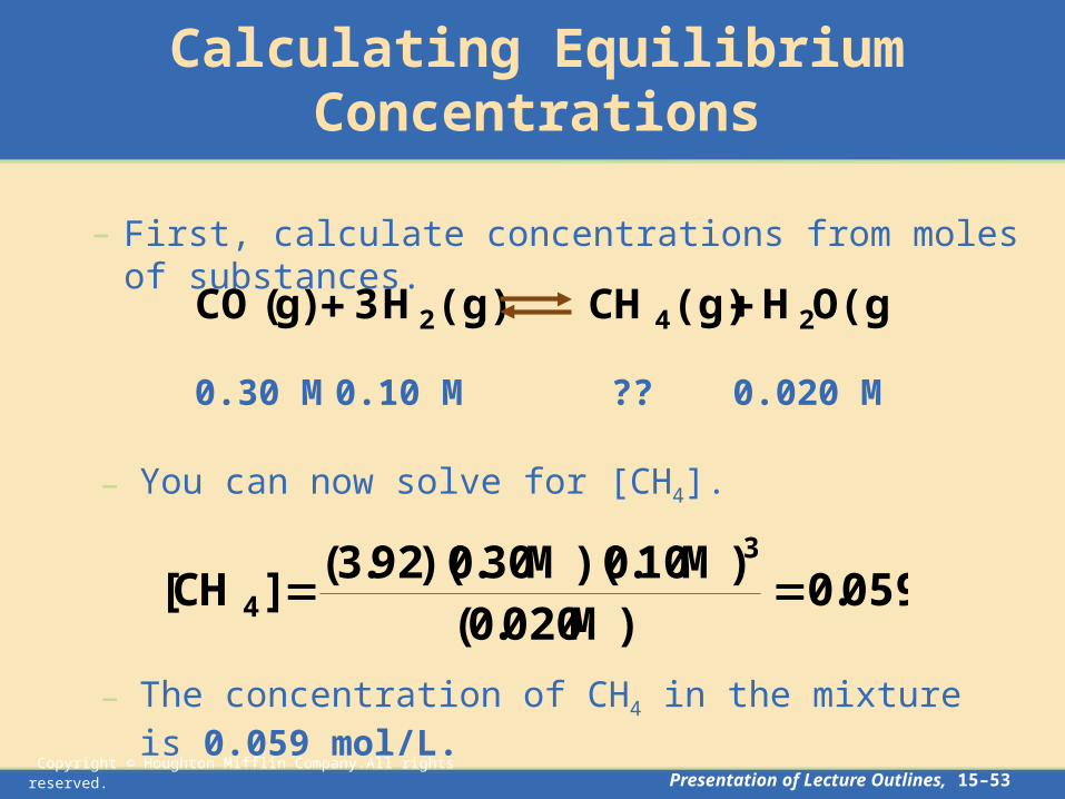
O(g)H (g)CH (g)H 3 )g(CO 242

– For example, consider the following equilibrium.




0.30 mol1.0 L

0.10 mol1.0 L

0.020 mol1.0 L??

O(g)H (g)CH (g)H 3 )g(CO 242



??0.30 M 0.10 M 0.020 M

– The equilibrium-constant expression is:

32

24c ]H][CO[

]OH][CH[K

O(g)H (g)CH (g)H 3 )g(CO 242




– Substituting the known concentrations and the value of Kc gives:

34

)M10.0)(M30.0(

)M020.0](CH[92.3

??0.30 M 0.10 M 0.020 M

O(g)H (g)CH (g)H 3 )g(CO 242




– You can now solve for [CH4].

059.0)M020.0(

)M10.0)(M30.0)(92.3(]CH[

3

4

– The concentration of CH4 in the mixture is 0.059 mol/L.

??0.30 M 0.10 M 0.020 M


O(g)H (g)CH (g)H 3 )g(CO 242



• Suppose we begin a reaction with known amounts of starting materials and want to calculate the quantities at equilibrium.




• Suppose you start with 1.000 mol each of carbon monoxide and water in a 50.0 L container. Calculate the molarity of each substance in the equilibrium mixture at 1000 oC.

• Kc for the reaction is 0.58 at 1000 oC.

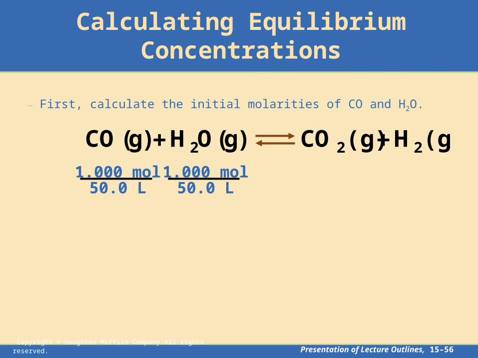
(g)H(g)CO )g(OH)g(CO 222



– First, calculate the initial molarities of CO and H2O.

1.000 mol50.0 L

1.000 mol50.0 L




• The starting concentrations of the products are 0.• We must now set up a table of concentrations (starting, change,

and equilibrium expressions in x).

0.0200 M 0.0200 M 0 M 0 M

– First, calculate the initial molarities of CO and H2O.




– Let x be the moles per liter of product formed.

Starting 0.0200 0.0200 0 0

Change -x -x +x +x

Equilibrium 0.0200-x 0.0200-x x x


]OH][CO[]H][CO[

K2

22c




– Solving for x.

Starting 0.0200 0.0200 0 0Change -x -x +x +x

Equilibrium0.0200-x 0.0200-x x x

– Substituting the values for equilibrium concentrations, we get:

)x0200.0)(x0200.0()x)(x(

58.0




– Solving for x.



– Or:

2

2

)x0200.0(

x58.0




– Solving for x.



– Taking the square root of both sides we get:

)x0200.0(x

76.0




– Solving for x.



– Rearranging to solve for x gives:

0086.076.1

76.00200.0x




– Solving for equilibrium concentrations.



– If you substitute for x in the last line of the table you obtain the following equilibrium concentrations.

0.0114 M CO0.0114 M H2O 0.0086 M H2

0.0086 M CO2




• The preceding example illustrates the three steps in solving for equilibrium concentrations.

1. Set up a table of concentrations (starting, change, and equilibrium expressions in x).

2. Substitute the expressions in x for the equilibrium concentrations into the equilibrium-constant equation.

3. Solve the equilibrium-constant equation for the values of the equilibrium concentrations.



• In some cases it is necessary to solve a quadratic equation to obtain equilibrium concentrations.

• The next example illustrates how to solve such an equation.




• Suppose 1.00 mol H2 and 2.00 mol I2 are placed in a 1.00-L vessel. How many moles per liter of each substance are in the gaseous mixture when it comes to equilibrium at 458 oC?

• Kc at this temperature is 49.7.

HI(g)2 )g(I)g(H 22



– The concentrations of substances are as follows.

Starting 1.00 2.00 0

Change -x -x +2x

Equilibrium 1.00-x 2.00-x 2x


]I][H[]HI[

K22

2

c

HI(g)2 )g(I)g(H 22



– The concentrations of substances are as follows.

Starting 1.00 2.00 0

Change -x -x +2x


– Substituting our equilibrium concentration expressions gives:

)x00.2)(x00.1()x2(

K2

c

HI(g)2 )g(I)g(H 22



– Solving for x.

– Because the right side of this equation is not a perfect square, you must solve the quadratic equation.

HI(g)2 )g(I)g(H 22 Starting 1.00 2.00 0

Change -x -x +2x




– Solving for x.

– The equation rearranges to give:


Change -x -x +2x


000.2x00.3x920.0 2



– Solving for x.

– The two possible solutions to the quadratic equation are:


Change -x -x +2x


0.93x and 33.2x



– Solving for x.

– However, x = 2.33 gives a negative value to 1.00 - x (the equilibrium concentration of H2), which is not possible.


Change -x -x +2x


remains. 0.93Only x



• Solving for equilibrium concentrations.

– If you substitute 0.93 for x in the last line of the table you obtain the following equilibrium concentrations.

0.07 M H2 1.07 M I2 1.86 M HI


Change -x -x +2x



Le Chatelier’s Principle

• Obtaining the maximum amount of product from a reaction depends on the proper set of reaction conditions.

– Le Chatelier’s principle states that when a system in a chemical equilibrium is disturbed by a change of temperature, pressure, or concentration, the equilibrium will shift in a way that tends to counteract this change.


Removing Products or Adding Reactants

• Let’s refer back to the illustration of the U-tube in the first section of this chapter.

– It’s a simple concept to see that if we were to remove products (analogous to dipping water out of the right side of the tube) the reaction would shift to the right until equilibrium was reestablished.



Removing Products or Adding Reactants

• Let’s refer back to the illustration of the U-tube in the first section of this chapter.

– Likewise, if more reactant is added (analogous to pouring more water in the left side of the tube) the reaction would again shift to the right until equilibrium is reestablished.



Effects of Pressure Change

• A pressure change caused by changing the volume of the reaction vessel can affect the yield of products in a gaseous reaction only if the reaction involves a change in the total moles of gas present (see Figure 15.12).



• If the products in a gaseous reaction contain fewer moles of gas than the reactants, it is logical that they would require less space.

• So, reducing the volume of the reaction vessel would, therefore, favor the products.

• Conversely, if the reactants require less volume (that is, fewer moles of gaseous reactant), then decreasing the volume of the reaction vessel would shift the equilibrium to the left (toward reactants).



• Literally “squeezing” the reaction will cause a shift in the equilibrium toward the fewer moles of gas.

• It’s a simple step to see that reducing the pressure in the reaction vessel by increasing its volume would have the opposite effect.

• In the event that the number of moles of gaseous product equals the number of moles of gaseous reactant, vessel volume will have no effect on the position of the equilibrium.


Effect of Temperature Change

• Temperature has a significant effect on most reactions (see Figure 15.13).– Reaction rates generally increase with an increase

in temperature. Consequently, equilibrium is established sooner.

– In addition, the numerical value of the equilibrium constant Kc varies with temperature.



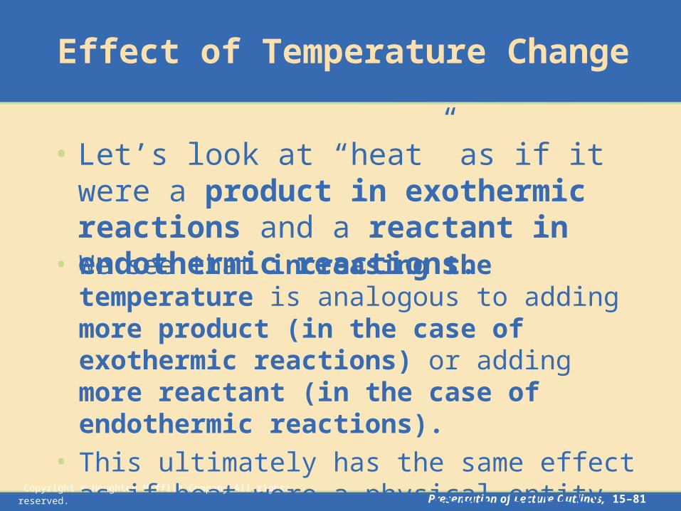
• Let’s look at “heat” as if it were a product in exothermic reactions and a reactant in endothermic reactions.

• We see that increasing the temperature is analogous to adding more product (in the case of exothermic reactions) or adding more reactant (in the case of endothermic reactions).

• This ultimately has the same effect as if heat were a physical entity.



• For example, consider the following generic exothermic reaction.

• Increasing temperature would be analogous to adding more product, causing the equilibrium to shift left.

• Since “heat” does not appear in the equilibrium-constant expression, this change would result in a smaller numerical value for Kc.

negative) is H( heat""products reactants



• For an endothermic reaction, the opposite is true.

• Increasing temperature would be analogous to adding more reactant, causing the equilibrium to shift right.

• This change results in more product at equilibrium, amd a larger numerical value for Kc.

positive) is H( products reactantsheat""



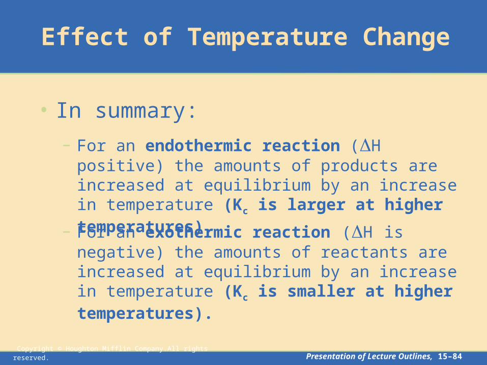
• In summary:

– For an exothermic reaction (H is negative) the amounts of reactants are increased at equilibrium by an increase in temperature (Kc is smaller at higher temperatures).

– For an endothermic reaction (H positive) the amounts of products are increased at equilibrium by an increase in temperature (Kc is larger at higher temperatures).


Effect of a Catalyst

• A catalyst is a substance that increases the rate of a reaction but is not consumed by it.

– It is important to understand that a catalyst has no effect on the equilibrium composition of a reaction mixture (see Figure 15.15).

– A catalyst merely speeds up the attainment of equilibrium.


Operational Skills

• Applying stoichiometry to an equilibrium mixture

• Writing equilibrium-constant expressions• Obtaining the equilibrium constant from

reaction composition• Using the reaction quotient• Obtaining one equilibrium concentration given

the others


Operational Skills

• Solving equilibrium problems

• Applying Le Chatelier’s principle


Figure 15.3: Catalytic methanation reaction approaches equilibrium.

Return to Slide 3


Animation: Equilibrium Decomposition of N2O4

Return to Slide 15

(Click here to open QuickTime animation)


Figure 15.5: Some equilibrium compositions for the methanation reaction.

Return to Slide 20


Return to Slide 21



Return to Slide 22



Return to Slide 23



Return to Slide 24



Return to Slide 25



Return to Slide 26



Return to Slide 27



Figure 15.6: The concentration of a gas at a given temperature is proportional to the pressure.

Return to Slide 28


Animation: Pressure and Concentration of a Gas

Return to Slide 28

(Click here to open QuickTime animation)


Figure 15.12 A-C

Return to Slide 77


Figure 15.13: The effect of changing the temperature on chemical equilibrium. Photo courtesy of

American Color.

Return to Slide 80


Figure 15.15: Oxidation of ammonia using a copper catalyst.

Photo courtesy of James Scherer.

Return to Slide 85

Documents

Chemical Equilibrium. Copyright © Houghton Mifflin Company.All rights reserved. Presentation of Lecture Outlines, 15–2 Chemical Equilibrium When compounds