HAL Id: hal-03002057https://hal.archives-ouvertes.fr/hal-03002057

Submitted on 12 Nov 2020

HAL is a multi-disciplinary open accessarchive for the deposit and dissemination of sci-entific research documents, whether they are pub-lished or not. The documents may come fromteaching and research institutions in France orabroad, or from public or private research centers.

L’archive ouverte pluridisciplinaire HAL, estdestinée au dépôt et à la diffusion de documentsscientifiques de niveau recherche, publiés ou non,émanant des établissements d’enseignement et derecherche français ou étrangers, des laboratoirespublics ou privés.

Chemical Composition of Hexene-Based LinearLow-Density Polyethylene by Infrared Spectroscopy and

ChemometricsOlivier Boyron, Manel Taam, Christophe Boisson

To cite this version:Olivier Boyron, Manel Taam, Christophe Boisson. Chemical Composition of Hexene-Based Lin-ear Low-Density Polyethylene by Infrared Spectroscopy and Chemometrics. Macromolecular Chem-istry and Physics, Wiley-VCH Verlag, 2019, 220 (24), pp.1900376. �10.1002/macp.201900376�. �hal-03002057�

- 1 -

Chemical Composition of Hexene Based LLDPE by Infrared Spectroscopy and

Chemometrics

Olivier Boyron*, Manel Taam, Christophe Boisson

–––––––––

Université de Lyon, Univ. Lyon 1, CPE Lyon, CNRS UMR 5265, Laboratoire de Chimie Catalyse

Polymères et Procédés (C2P2), Equipe LCPP, Bat 308F, 43 Bd du 11 Novembre 1918, F-69616

Villeurbanne, France

E-mail : olivier.boyron@univ-lyon1.fr

Keywords: infrared; near infrared; ethylene-1-hexene copolymer; LLDPE; chemometrics

Abstract

Mid and near infrared (MIR and NIR) spectroscopy associated with the partial least squares

(PLS) method makes it possible to rapidly characterize the composition of linear low-density

polyethylene (LLDPE) in a large range of 1-hexene content from 0 to 21 mol%. LLDPEs are

produced using zirconocene catalysts activated with methylaluminoxane. PLS regression

methods for MIR and NIR are constructed from this series of LLDPEs to quantify the 1-hexene

content in unknown copolymers. In this case, the PLS regression method aims to correlate the

1-hexene content in the copolymers with their IR spectra. Multivariate calibration models are

constructed by the PLS algorithm on pretreated data of MIR and NIR analyses. They are tested

and validated by comparing results obtained by NMR and the PLS analyses for four unknown

ethylene-1-hexene copolymers.

1. Introduction

- 2 -

With an annual global production of approximately 100 million tons, polyethylenes (PEs) are

the main commercial polymeric materials.[1, 2] They are typically classified into three main

families such as high-density polyethylene (HDPE; 0.940 to 0.970 g/cm3), low-density

polyethylene (LDPE; 0.910 to 0.940 g/cm3) and linear low-density polyethylene (LLDPE;

0.916 to 0.940 g/cm3). HDPE has no or only a small amount of branching (SCB), LDPE

contains a combination of long (>C6) and short chain branching, while the branching in LLDPE

is predominantly from short chain branching. This last one is synthetized by copolymerization

of ethylene and an α-olefin which allows the insertion of a short-chain branching into the main

chain and thus impacts the crystallinity of the material.[3] The frequently used α-olefins are 1-

butene, 1-hexene and 1-octene.[1, 4] The crystallinity and then the physical properties of LLDPE

can be adjusted using different content of comonomer.[5, 6] Consequently, it is highly relevant

to quantify the amount of comonomer units incorporated into LLDPE during the polymerization

process.

Various analytical techniques have been developed to quantify the short chain branching

content. It has been widely investigated using spectroscopy like Fourier transform infrared

(FTIR)[7-10], proton and carbon nuclear magnetic resonance (H-NMR and 13C-NMR)[11-14].

Liquid chromatography based on crystallibility of polyolefins has been established by Wild,

Monrabal, Soares and Pasch through temperature rising elution fractionation (TREF)[15-19] and

crystallization analysis fractionation (CRYSTAF)[20, 21]. However, these techniques cannot be

used for the separation of amorphous fractions of the polymers. The combination of high

temperature liquid chromatography with a Hypercarb column operating with a temperature

gradient [22-27] was introduced by Cong and Macko and allow the analysis of amorphous

polymers. These high temperature fractionation techniques were able to determine the chemical

composition distribution (CCD) of LLDPE. In addition, thermal analysis coupled with mass

- 3 -

spectrometry[28-31] has been employed to measure the branching type and the content of α-

olefins in LLDPE.

However, these approaches are time consuming due to the sample preparation (dissolution at

high temperature with toxic solvent) for most techniques and the time required to record and

process the data. In many instances, for example in the case of high throughput experiments or

during recycling process, it is desirable to determine the polymer composition in a shorter time.

Infrared spectroscopy is a consistent and an essential analytical method for exploring polymer

composition.[32, 33] More specifically, Fourier transform infrared spectroscopy in attenuated

total reflection mode (ATR-FTIR)[34-36] and near infrared (NIR)[37-39] equipped with an

integrating sphere might be advantageous for measuring the chemical composition of LLDPE

as inexpensive sample preparation is sufficient for theses technique. While many previous

studies[9, 40, 41] are based on absorbance attributable to branch type there are few publications on

quantitative studies.[7, 42, 43] In work of Blitz and McFaddin,[7] FTIR calibration for different

branch type (methyl, ethyl, butyl, hexyl) in LLDPE based on absorption of only one wavelength

was reported. Sano et al and Shimoyama et al described methods to predict density in LLDPE

by applying chemometrics tools to Raman spectra[42] and near IR spectra[43]. In this present

study we propose to calibrate IR analysis of LLDPE with a large and complete set of polymers

up to 21 mol% of 1-hexene and with multiple absorption bands in order to increase the

robustness and precision of the method.

Because structural changes in ethylene-1-hexene copolymers cause low modifications in MIR

and NIR spectra, the use of chemometrics techniques are required to highlight differences in

polymer spectra. Partial least-squares (PLS) regression is commonly used to improve the

resolution in analytical signals that can be overlaid for intricate materials.[44-48] In particular, we

demonstrated, in a previous work, that PLS regression can be efficiently used for quantitative

determination of composition of ethylene-butadiene copolymers.[49]

- 4 -

This work proposes an original method based on infrared spectroscopy and chemometrics.

Firstly, copolymers containing various proportions of 1-hexene were synthetized using the

zirconocene catalyst.[50-52] Secondly, the average composition of the copolymers was measured

using 1H and 13C-NMR spectroscopy. The homogeneity in molar mass and chemical

composition was also controlled by high temperature size exclusion chromatography (HT-SEC)

and thermal gradient interaction chromatography (TGIC). Subsequently, the copolymers were

used to construct the PLS model with NIR and MIR data.

2. Experimental Section

2.1. Polymerization method

All manipulations were performed under dry argon, using standard Schlenk techniques and

glovebox. 1-hexene was dried over CaH2 prior to use. Toluene and heptane were dried on 3 Å

molecular sieves. Methyl-aluminoxane (MAO) 10% wt. in toluene was purchased from Aldrich

and triethylaluminium (AlEt3) was purchased from Albemarle and used as heptane solution (1

M). Ethylene (99.5%) from Air Liquide was purified by passing on three successive columns

containing respectively molecular sieves, alumina and a copper catalyst. The metallocene

complexes rac-Et(Ind)2ZrCl2 and (nBuCp)2ZrCl2 were purchased from Sigma-Aldrich. The

activating support was prepared as described in previous work.[53]

Ethylene polymerizations were performed in a 500 ml glass reactor equipped with a stainless-

steel blade stirrer and an external water jacket to control the temperature. MAO and the required

amounts of 1-hexene were introduced in a flask containing 300 mL of heptane. The mixture

was transferred in the reactor under a stream of argon. The argon was then pumped out before

introducing the ethylene or a mixture of ethylene/propene. Temperature and pressure were then

progressively increased up to 80 °C and 3.8 x 105 Pa. 100 µL of a solution (1.5 mM in toluene)

of rac-Et(Ind)2ZrCl2 and (nBuCp)2ZrCl2 were then introduced in the reactor under 4 x 105 Pa

- 5 -

of ethylene to start the polymerization. The pressure was kept constant at 4 x 105 Pa during the

polymerization. After 30 minutes of reaction, the polymerization was stopped by releasing the

pressure and cooling down the reactor to the room temperature. The resulting mixture was

poured in 400 mL of methanol. The polymer was collected by filtration, washed with methanol

and dried under vacuum.

In the case of slurry polymerization using the supported rac-Et(Ind)2ZrCl2 catalyst, a similar

procedure was used. However the Al(i-Bu)3 (1 M solution in heptane), the activating support,

the metallocene precatalyst (1 mM solution in toluene), and 1-hexene were introduced

successively in the flask containing 300 mL of heptane. The mixture was transferred in the

reactor and the polymerization started by pressurization of the reactor to 4 x 105 Pa.

2.2. Characterization

2.2.1. High temperature size exclusion chromatography

High temperature size exclusion chromatography (HT-SEC) analyses were performed using a

Viscotek system, from Malvern Instruments, equipped with a combination of three columns

(PLgel Olexis from Agilent Technologies, 300 mm × 7.5 mm, 13µm). Samples were dissolved

in 1,2,4-trichlorobenzene (TCB) with a concentration of 5 mg mL-1 by heating the mixture for

1 h at 150°C. 200 µL of sample solutions were injected and eluted with 1,2,4-TCB using a flow

rate of 1 mL min-1 at 150 °C. 2,6-di-tert-butyl-4-methylphenol (BHT) was added to the eluent

(200 mg L-1) in order to stabilize the polymer against oxidative degradation. Online detection

was performed with a differential refractive-index detector and a dual light-scattering detector

(LALS and RALS) for absolute molar mass determination. OmniSEC software version 5.2 was

used for data acquisition and calculation.

2.2.2. Thermal Gradient Interaction Chromatography

- 6 -

TGIC experiments were performed using an instrument from PolymerChar (Valencia, Spain)

to characterize the composition distribution in samples. The instrument was equipped with a

Hypercarb column from Thermo Scientific. The samples were dissolved in 10 mL vials for 1 h

at 150 °C with 1,2,4 trichlorobenzene (TCB) containing 300 ppm of BHT and purge with

nitrogen to protect the polymer against oxidative degradation. 200 µL of sample solution at a

concentration of 1 mg mL−1 were injected into the column at 150 °C. This technique requires a

cooling (adsorption) and a heating (desorption) step. A cooling ramp of 20 °C min−1 down to

40 °C was applied to promote polymer adsorption. Elution begins isothermally at 40 °C during

5 min at a flow rate of 0.5 mL min−1 followed by a heating ramp at 2 °C min−1 to desorb the

polymer. An infrared detector was used to monitor the components’ concentration and

composition when the chains were eluted from the column.

Because TGIC separates by adsorption it has the possibility to extend the range of polymers to

be analyzed towards the amorphous region which is limited by crystallization techniques

(TREF, CRYSTAF). Then, LLDPE with high content of comonomer can be separated.

2.2.3. Nuclear magnetic resonance spectroscopy

Co-monomer contents of copolymers were determined by NMR using a Bruker Avance III 400

spectrometer operating at 400 MHz for 1H-NMR and 100.6 MHz for 13C-NMR. 1H-NMR

spectra were obtained with a 5mm QNP probe at 373 K and the 13C-NMR spectra were obtained

with a 10 mm PA-SEX probe at 373 K. A 3:1 volume mixture of 1, 2, 4-trichlorobenzene and

toluene-d8 was used as solvent. The chemical shifts were measured in ppm using for 1H-NMR

the reference of toluene (CHD2 at 2.185 ppm) and for 13C-NMR the resonance of the major

backbone methylene carbon resonance (CH2 at 30.00 ppm) as internal references.

2.2.4. Mid infrared spectroscopy

- 7 -

Mid infrared (MIR) spectra were recorded using a Nicolet iS50 Fourier transform infrared

(FTIR) spectrometer from Thermo Fisher Scientific. The spectrometer was equipped with an

attenuated total reflection (ATR) module (single-bounce diamond crystal) and a deuterated

triglycine sulfate detector and KBr optics. Before each measurement, the diamond crystal was

carefully cleaned with ethanol and dried in ambient air. A small amount of sample in powder

state was pressed directly on the diamond crystal with a constant pressure of 7 x 107 Pa.

Background and sample were acquired using 32 scans at a spectral resolution of 4 cm-1 from 4

000 to 400 cm-1. Spectral data were obtained with OMNIC Software from Thermo Fisher

Scientific. The ATR spectra were not corrected for pathlength. Three replicates for each sample

were made and compared. If they were similar, only one spectrum was selected and used for

the model. They were different for one sample and it was not used in this work.

2.2.5. Near infrared spectroscopy

Near infrared (NIR) spectra were collected using a Nicolet iS50 FTIR spectrometer from

Thermo Fisher Scientific under nitrogen. The spectrometer was equipped with an integrating

sphere (Thermo Scientific Smart NIR).

The synthetized LLDPE gives, for some of them, a heterogeneous powder agglomeration.

Working on the raw samples was difficult and a second method using a solvent to dissolve

samples was also performed. To obtain a homogenous solution, 40 mg of polymer in 200 µL

of 1,2,4-TCB, with BHT as stabilizer, was dissolved in a 2 ml vial. Then the vials were heated

up to 150 °C for 1 hour in order to entirely dissolve the sample. Since glass does not absorb in

NIR the samples were analyzed directly through the vials.

Background and samples were acquired using 32 scans at a spectral resolution of 4 cm−1 from

11 000 to 3 800 cm-1. Spectral data were obtained with OMNIC Software from Thermo Fisher

Scientific.

- 8 -

2.2.6. Chemometrics tools

Chemometric analyse of NIR and MIR spectra were achieved using a partial least squares (PLS)

method with two different softwares. TQ Analyst software from Thermo Fisher Scientific and

The Unscrambler X 10.5.1 software from Camo were used to analyze NIR and MIR data,

construct the models and quantify the unknown samples.

3. Results and discussion

3.1. Chemical composition of ethylene-1-hexene copolymers

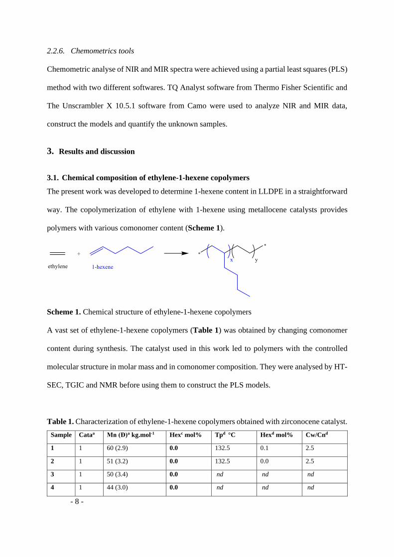
The present work was developed to determine 1-hexene content in LLDPE in a straightforward

way. The copolymerization of ethylene with 1-hexene using metallocene catalysts provides

polymers with various comonomer content (Scheme 1).

Scheme 1. Chemical structure of ethylene-1-hexene copolymers

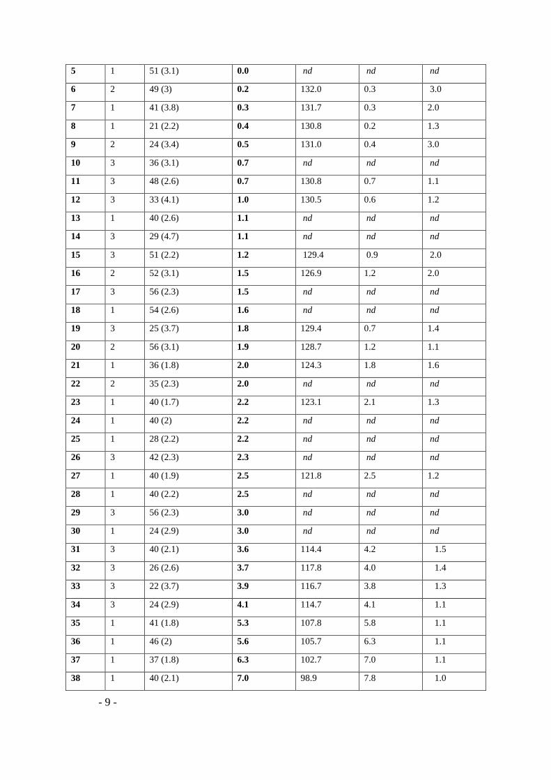
A vast set of ethylene-1-hexene copolymers (Table 1) was obtained by changing comonomer

content during synthesis. The catalyst used in this work led to polymers with the controlled

molecular structure in molar mass and in comonomer composition. They were analysed by HT-

SEC, TGIC and NMR before using them to construct the PLS models.

Table 1. Characterization of ethylene-1-hexene copolymers obtained with zirconocene catalyst.

Sample Cataa Mn (Ɖ)a kg.mol-1 Hexc mol% Tpd °C Hexd mol% Cw/Cnd

1 1 60 (2.9) 0.0 132.5 0.1 2.5

2 1 51 (3.2) 0.0 132.5 0.0 2.5

3 1 50 (3.4) 0.0 nd nd nd

4 1 44 (3.0) 0.0 nd nd nd

- 9 -

5 1 51 (3.1) 0.0 nd nd nd

6 2 49 (3) 0.2 132.0 0.3 3.0

7 1 41 (3.8) 0.3 131.7 0.3 2.0

8 1 21 (2.2) 0.4 130.8 0.2 1.3

9 2 24 (3.4) 0.5 131.0 0.4 3.0

10 3 36 (3.1) 0.7 nd nd nd

11 3 48 (2.6) 0.7 130.8 0.7 1.1

12 3 33 (4.1) 1.0 130.5 0.6 1.2

13 1 40 (2.6) 1.1 nd nd nd

14 3 29 (4.7) 1.1 nd nd nd

15 3 51 (2.2) 1.2 129.4 0.9 2.0

16 2 52 (3.1) 1.5 126.9 1.2 2.0

17 3 56 (2.3) 1.5 nd nd nd

18 1 54 (2.6) 1.6 nd nd nd

19 3 25 (3.7) 1.8 129.4 0.7 1.4

20 2 56 (3.1) 1.9 128.7 1.2 1.1

21 1 36 (1.8) 2.0 124.3 1.8 1.6

22 2 35 (2.3) 2.0 nd nd nd

23 1 40 (1.7) 2.2 123.1 2.1 1.3

24 1 40 (2) 2.2 nd nd nd

25 1 28 (2.2) 2.2 nd nd nd

26 3 42 (2.3) 2.3 nd nd nd

27 1 40 (1.9) 2.5 121.8 2.5 1.2

28 1 40 (2.2) 2.5 nd nd nd

29 3 56 (2.3) 3.0 nd nd nd

30 1 24 (2.9) 3.0 nd nd nd

31 3 40 (2.1) 3.6 114.4 4.2 1.5

32 3 26 (2.6) 3.7 117.8 4.0 1.4

33 3 22 (3.7) 3.9 116.7 3.8 1.3

34 3 24 (2.9) 4.1 114.7 4.1 1.1

35 1 41 (1.8) 5.3 107.8 5.8 1.1

36 1 46 (2) 5.6 105.7 6.3 1.1

37 1 37 (1.8) 6.3 102.7 7.0 1.1

38 1 40 (2.1) 7.0 98.9 7.8 1.0

- 10 -

39 1 60 (4.1) 9.0 nd nd nd

40 1 56 (2) 13.6 77.4 13.1 1.2

41 1 31 (1.4) 20.7 53.6 19.0 1.0

a catalytic systems based on the complexes [1] rac-Et(Ind)2ZrCl2 and [2] (nBuCp)2ZrCl2 [3]

supported rac-Et(Ind)2ZrCl2 used for the preparation of ethylene-1-hexene samples.b Number

average molar mass and dispersity obtained with HT-SEC, c 1-hexene content determined with

1H NMR and 13C NMR, delution peak temperature, 1-hexene content and dispersity of chemical

composition obtained by TGIC, nd not determined

3.2. Interpretation of NMR spectra

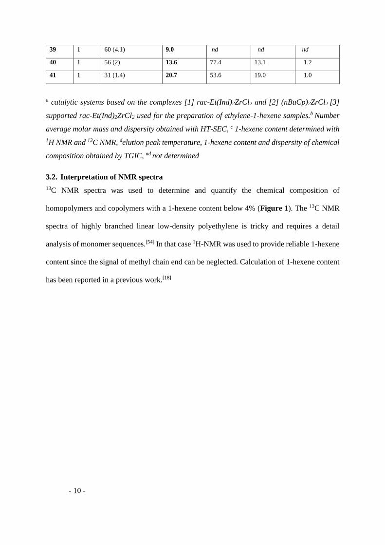
13C NMR spectra was used to determine and quantify the chemical composition of

homopolymers and copolymers with a 1-hexene content below 4% (Figure 1). The 13C NMR

spectra of highly branched linear low-density polyethylene is tricky and requires a detail

analysis of monomer sequences.[54] In that case 1H-NMR was used to provide reliable 1-hexene

content since the signal of methyl chain end can be neglected. Calculation of 1-hexene content

has been reported in a previous work.[18]

- 11 -

Figure 1. 13C NMR spectra (TCB/ toluene-d8, 363 K) of sample 23 with 2,2 mol% of 1-hexene,

a), resonance region of 1H NMR spectra (TCB/ toluene-d8, 363 K) of sample 40 with 13,6

mol% of 1-hexene b).

3.3. Chemical composition distribution

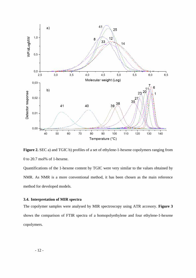
The molar masses and the dispersity of samples are reported in Table 1. The SEC profiles, in

Figure 2a, show a unimodal molar masses distribution. The TGIC peak of the samples elutes

in decreasing order of comonomer content, as observed in previous works.[24, 27, 55-58] The

elution temperature of 11 samples, issue from homogeneous catalyst [1, 2] and supported

catalyst [3], were plotted (Figure 2b). The peaks are rather narrow and have a similar

distribution to a Gaussian which confirms that all polymers were quite homogeneous in

composition.

1.001.051.101.151.201.251.301.351.401.451.501.551.601.651.701.751.801.851.901.952.002.052.10 ppm

1.062

1.442

15161718192021222324252627282930313233343536373839 ppm

14.15

23.38

27.20

29.42

30.00

30.47

33.98

34.36

37.98

- 12 -

Figure 2. SEC a) and TGIC b) profiles of a set of ethylene-1-hexene copolymers ranging from

0 to 20.7 mol% of 1-hexene.

Quantifications of the 1-hexene content by TGIC were very similar to the values obtained by

NMR. As NMR is a more conventional method, it has been chosen as the main reference

method for developed models.

3.4. Interpretation of MIR spectra

The copolymer samples were analysed by MIR spectroscopy using ATR accesory. Figure 3

shows the comparison of FTIR spectra of a homopolyethylene and four ethylene-1-hexene

copolymers.

- 13 -

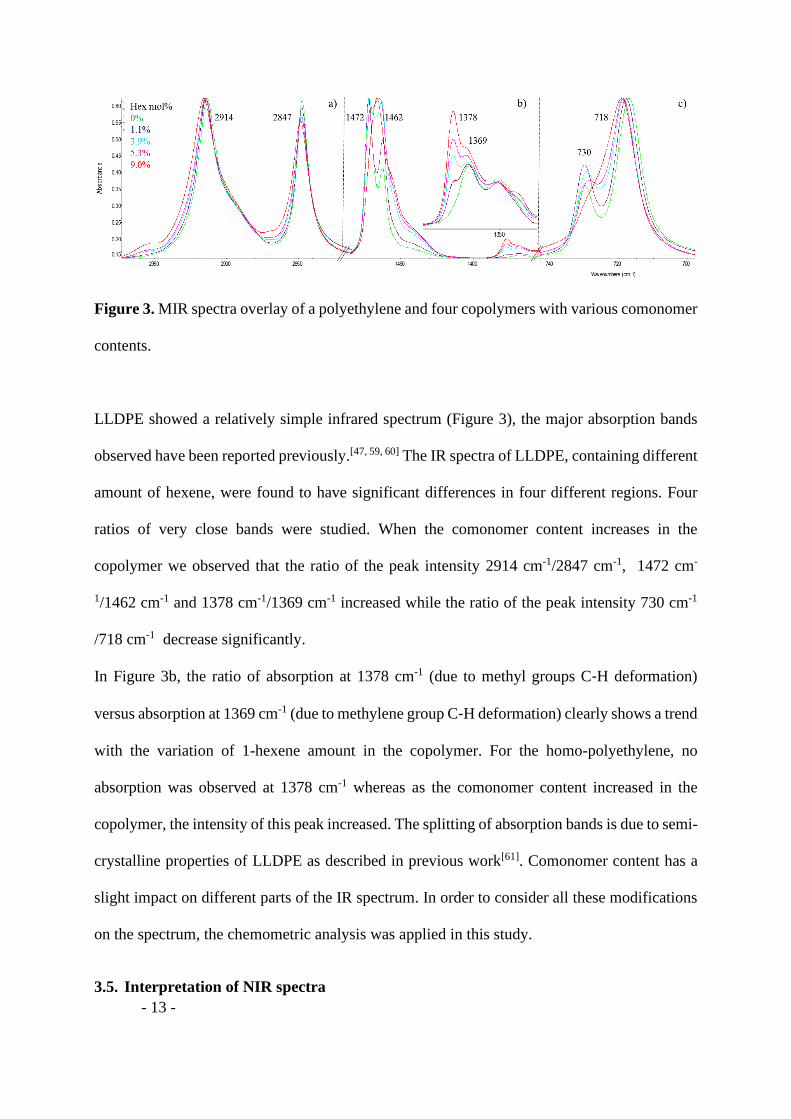
Figure 3. MIR spectra overlay of a polyethylene and four copolymers with various comonomer

contents.

LLDPE showed a relatively simple infrared spectrum (Figure 3), the major absorption bands

observed have been reported previously.[47, 59, 60] The IR spectra of LLDPE, containing different

amount of hexene, were found to have significant differences in four different regions. Four

ratios of very close bands were studied. When the comonomer content increases in the

copolymer we observed that the ratio of the peak intensity 2914 cm-1/2847 cm-1, 1472 cm-

1/1462 cm-1 and 1378 cm-1/1369 cm-1 increased while the ratio of the peak intensity 730 cm-1

/718 cm-1 decrease significantly.

In Figure 3b, the ratio of absorption at 1378 cm-1 (due to methyl groups C‐H deformation)

versus absorption at 1369 cm-1 (due to methylene group C‐H deformation) clearly shows a trend

with the variation of 1-hexene amount in the copolymer. For the homo-polyethylene, no

absorption was observed at 1378 cm-1 whereas as the comonomer content increased in the

copolymer, the intensity of this peak increased. The splitting of absorption bands is due to semi-

crystalline properties of LLDPE as described in previous work[61]. Comonomer content has a

slight impact on different parts of the IR spectrum. In order to consider all these modifications

on the spectrum, the chemometric analysis was applied in this study.

3.5. Interpretation of NIR spectra

- 14 -

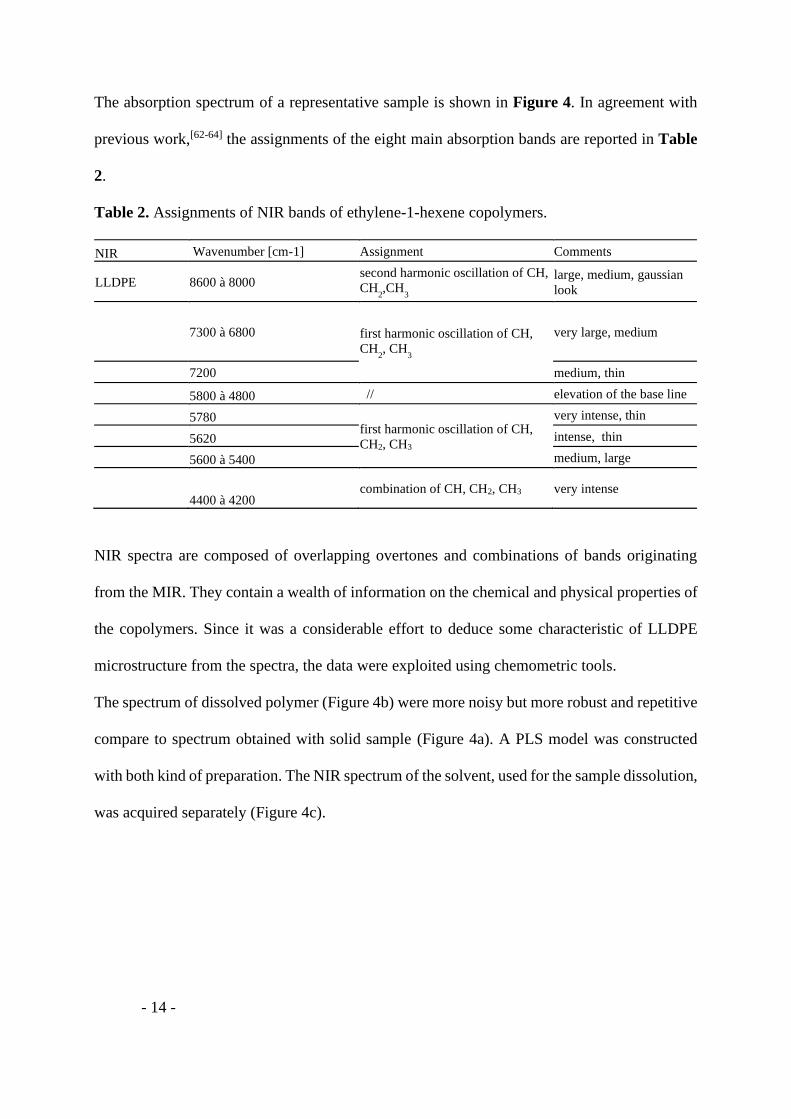
The absorption spectrum of a representative sample is shown in Figure 4. In agreement with

previous work,[62-64] the assignments of the eight main absorption bands are reported in Table

2.

Table 2. Assignments of NIR bands of ethylene-1-hexene copolymers.

NIR Wavenumber [cm-1] Assignment Comments

LLDPE 8600 à 8000 second harmonic oscillation of CH,

CH2,CH

3

large, medium, gaussian

look

7300 à 6800 first harmonic oscillation of CH,

CH2, CH

3

very large, medium

7200 medium, thin

5800 à 4800 // elevation of the base line

5780 first harmonic oscillation of CH,

CH2, CH3

very intense, thin

5620 intense, thin

5600 à 5400 medium, large

4400 à 4200 combination of CH, CH2, CH3 very intense

NIR spectra are composed of overlapping overtones and combinations of bands originating

from the MIR. They contain a wealth of information on the chemical and physical properties of

the copolymers. Since it was a considerable effort to deduce some characteristic of LLDPE

microstructure from the spectra, the data were exploited using chemometric tools.

The spectrum of dissolved polymer (Figure 4b) were more noisy but more robust and repetitive

compare to spectrum obtained with solid sample (Figure 4a). A PLS model was constructed

with both kind of preparation. The NIR spectrum of the solvent, used for the sample dissolution,

was acquired separately (Figure 4c).

- 15 -

Figure 4. NIR spectra of a copolymer (sample 12) a) in solid state b) dissolved in

trichlorobenzene and c) solvent alone.

3.6. Chemometric study

The goal of this work was to obtain a robust method to determine the 1-hexene content of an

unknown copolymer with MIR and NIR spectroscopy. A partial least squares regression (PLS)

model[44, 45, 65] was used.

3.6.1. Calibration set

In order to determine composition of an unknown ethylene-1-hexene copolymer, calibration

methods for MIR and for NIR were created with a set of 41 samples described above. The wide

range of composition of ethylene-1-hexene copolymers, from 0% to 20.7 mol%, was

particularly interesting for this purpose.

3.6.2. Performance index

The performance index (PI), that indicates the adequacy between the calculated polymer

compositions and NMR measurements, was chosen to measure the accuracy of the method. The

10000 9000 8000 7000 6000 5000

0.0

0.5

1.0

1.5A

bso

rba

nce

Wavenumber (cm-1)

a)

b)

c)

- 16 -

higher the performance index (up to 100) is, the better the agreement between calculated and

NMR values are. This parameter, reported for each method in Table 4, allowed us to decide

whether the modifications of the pre-processing data improve the accuracy of the method.

3.6.3. Prediction performance

The performance of the model was evaluated with the root mean square error of calibration

(RMSEC), the root mean square error of validation (RMSEV) and the correlation coefficient (r).

These values were reported in Table 4.

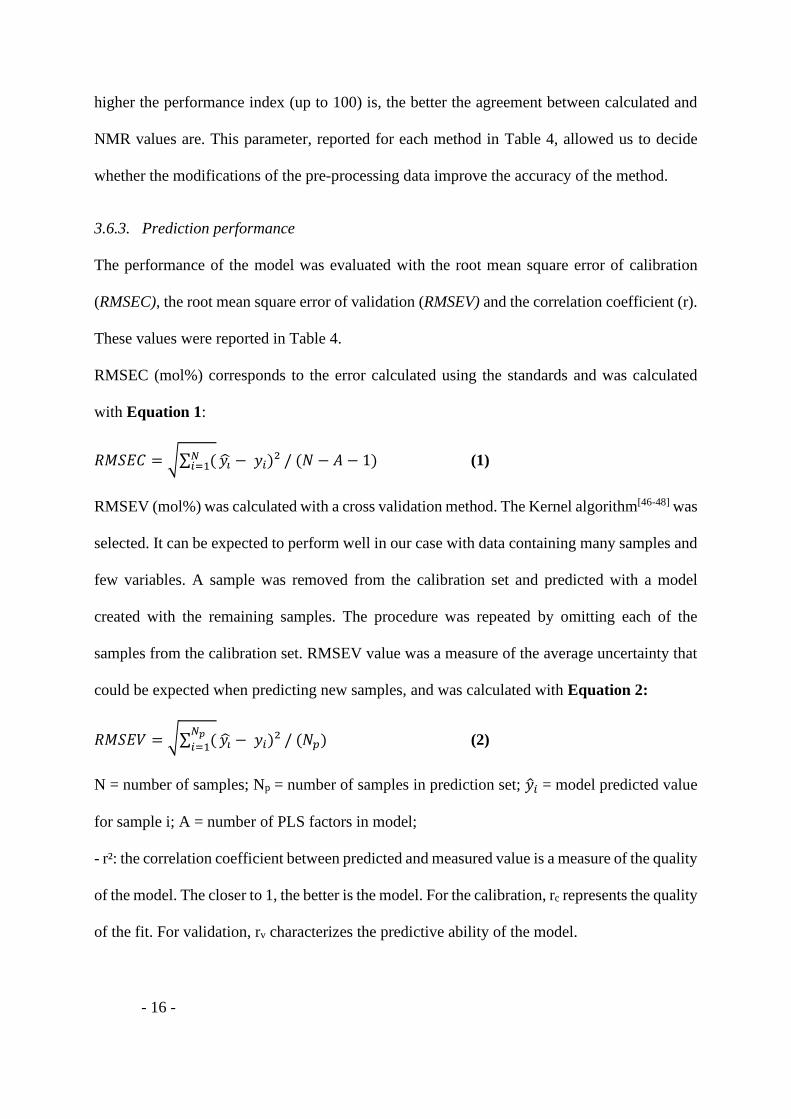
RMSEC (mol%) corresponds to the error calculated using the standards and was calculated

with Equation 1:

𝑅𝑀𝑆𝐸𝐶 = √∑ (𝑁𝑖=1 𝑦�̂� − 𝑦𝑖)² / (𝑁 − 𝐴 − 1) (1)

RMSEV (mol%) was calculated with a cross validation method. The Kernel algorithm[46-48] was

selected. It can be expected to perform well in our case with data containing many samples and

few variables. A sample was removed from the calibration set and predicted with a model

created with the remaining samples. The procedure was repeated by omitting each of the

samples from the calibration set. RMSEV value was a measure of the average uncertainty that

could be expected when predicting new samples, and was calculated with Equation 2:

𝑅𝑀𝑆𝐸𝑉 = √∑ (𝑁𝑝

𝑖=1𝑦�̂� − 𝑦𝑖)² / (𝑁𝑝) (2)

N = number of samples; Np = number of samples in prediction set; �̂�𝑖 = model predicted value

for sample i; A = number of PLS factors in model;

- r²: the correlation coefficient between predicted and measured value is a measure of the quality

of the model. The closer to 1, the better is the model. For the calibration, rc represents the quality

of the fit. For validation, rv characterizes the predictive ability of the model.

- 17 -

In order to validate the model, RMSEC and RMSEV values must be low and similar and r²

close to one.

3.6.4. Number of factors in PLS regression

The performance index plot was used to measure the divergence between the model and actual

data. It allows the determination of the PLS factor number (Table 4) to be used to properly

describe the variables. As the number of PLS factors increased, the performance index plot

increase. When the curve reaches its maximum, this value corresponds to the optimum number

of PLS factors. Including more PLS factors, the model will fit the calibration set better but can

lead to an ‘over-fitting’ of the model and to a poorer prediction for unknown sample. The choice

of four factor number in the calibration model was a balance between optimizing the explain

variance and limiting the model complexity.

3.6.5. Preprocessing method

Several data pre-processing methods were applied. The first derivate of the NIR and MIR

signals was chosen in order to reduce the baseline offset and the instrumental drift. In the

derivation process, noise can increase which requires a smoothing. The Savitzky-Golay

algorithm[66-68] was used for smoothing the signal and to reduce the impacts of varying baseline,

variable path lengths, and high stray lights due to scatter effects. A polynomial order of 2 and

a segment length of 7 points were applied. The pre-processing method was applied both to the

whole spectrum and to the spectral region selection.

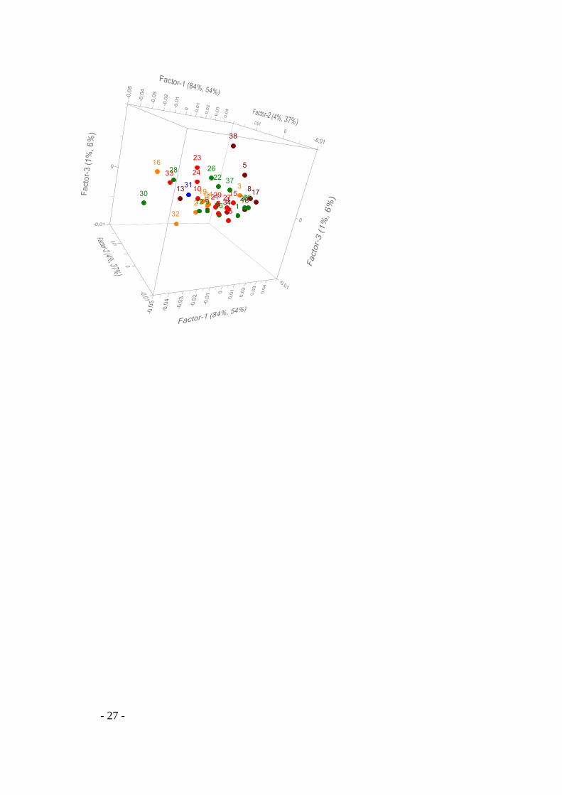
3.7. Scores

- 18 -

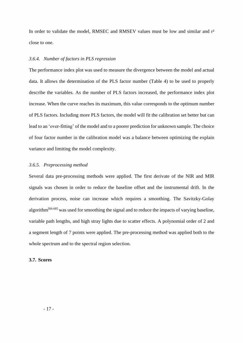
Figure 5. A principal component analysis (PCA) scores for factor 1 and factor 2 with

confidence intervals of 95% of a) MIR and b) NIR for ethylene-1-hexene copolymers sample.

Samples were disctinctly separated into four groups (blue, red, green and brown) depending of

1-hexene content (in mol%).

A principal component analysis (PCA) scores for factor 1 and factor 2, in Figure 5, summarized

more variation in the data than any other pair of components. The closer the samples were in

the score plot, the more similar they were. The plot for MIR (Figure 5a) and for NIR (Figure

5b) shows that when 1-hexene content increase, from blue to brown, the sample was clearly

shifted to the right. This means that the amount of comonomer had a real impact on the spectra

and that it could be measure using PLS regression. The scores plot shows that the separation of

the four regions of different hexene levels was better for the MIR model than for the NIR model.

The both score plot show that the sample 41 was considered as outlier. This sample was

different from the others, not because of an analytical error, but because of the high amount of

hexene. It was considered a false outlier and was not removed to preserve the large range of

analyses. Sample 41 was analyzed and used twice in the model to give more weight to this

sample which is located alone at the end of the calibration. In addition, the sigmoid-shaped

curvature of the score plots indicates that there were interactions between the predictors. Adding

more factor to the model would improve it.

3.7.1. Spectral region selection

- 19 -

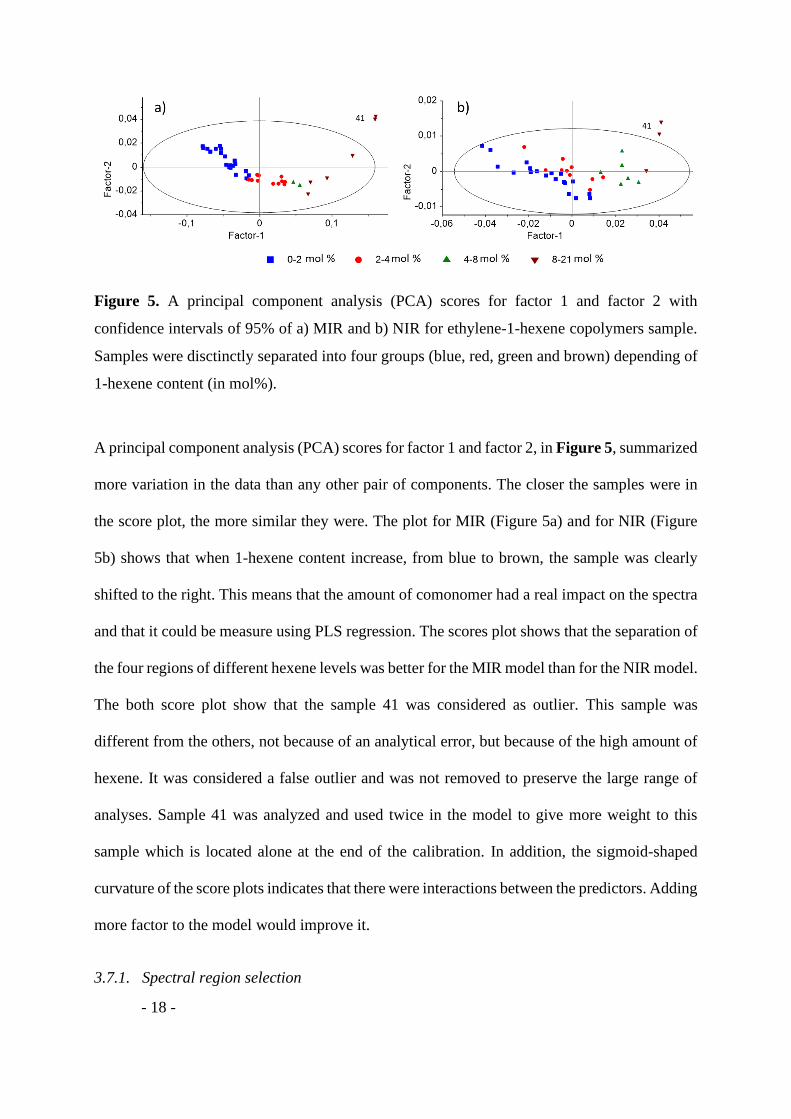
One approach was based on spectral region selection in which the wavelength with low

correlation were eliminated.

Figure 6. The contribution plot describes how individual variables contribute to the model, 3

spectral regions were clearly highlighted a) in MIR and b) in NIR. Variables represents the

wavelength in cm-1. The brackets indicate the wavelength ranges selected to be included in the

models.

In the contribution plot for MIR (Figure 6a), three spectral regions contribute significantly to

the discrimination. In order to improve the model and eliminate the wavelength likely

generating noise, we decided to select only the interesting spectral region: the bands from 3000

to 2750 cm-1, from 1500 to 1300 cm-1 and from 800 to 630 cm-1. This corresponds well to the

main absorption wavelengths of polyethylene (2914 cm-1, 2847 cm-1, 1472 cm-1, 1462 cm-1, 730

cm-1 and 718 cm-1) indicated in previous work.[49] For NIR, the contribution plot (Figure 6b)

made it possible to select the bands from 9000 to 7800 cm-1, from 6400 to 5400 cm-1 and from

4800 to 4000 cm-1. Although we observed an absorption between 7500 to 6900 cm-1, this range

- 20 -

was not selected in the model. The NIR model has been improved without the use of this range

mainly impacted by the solvent.

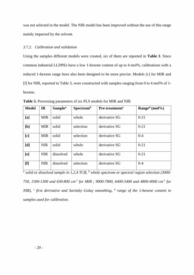
3.7.2. Calibration and validation

Using the samples different models were created, six of them are reported in Table 3. Since

common industrial LLDPEs have a low 1-hexene content of up to 4 mol%, calibrations with a

reduced 1-hexene range have also been designed to be more precise. Models [c] for MIR and

[f] for NIR, reported in Table 3, were constructed with samples ranging from 0 to 4 mol% of 1-

hexene.

Table 3. Processing parameters of six PLS models for MIR and NIR

Model IR Samplea Spectrumb Pre-treatmentc Ranged (mol%)

[a] MIR solid whole derivative SG 0-21

[b] MIR solid selection derivative SG 0-21

[c] MIR solid selection derivative SG 0-4

[d] NIR solid whole derivative SG 0-21

[e] NIR dissolved whole derivative SG 0-21

[f] NIR dissolved selection derivative SG 0-4

a solid or dissolved sample in 1,2,4 TCB, b whole spectrum or spectral region selection (3000-

750, 1500-1300 and 630-800 cm-1 for MIR ; 9000-7800, 6400-5400 and 4800-4000 cm-1 for

NIR), c first derivative and Savitzky–Golay smoothing, d range of the 1-hexene content in

samples used for calibration.

- 21 -

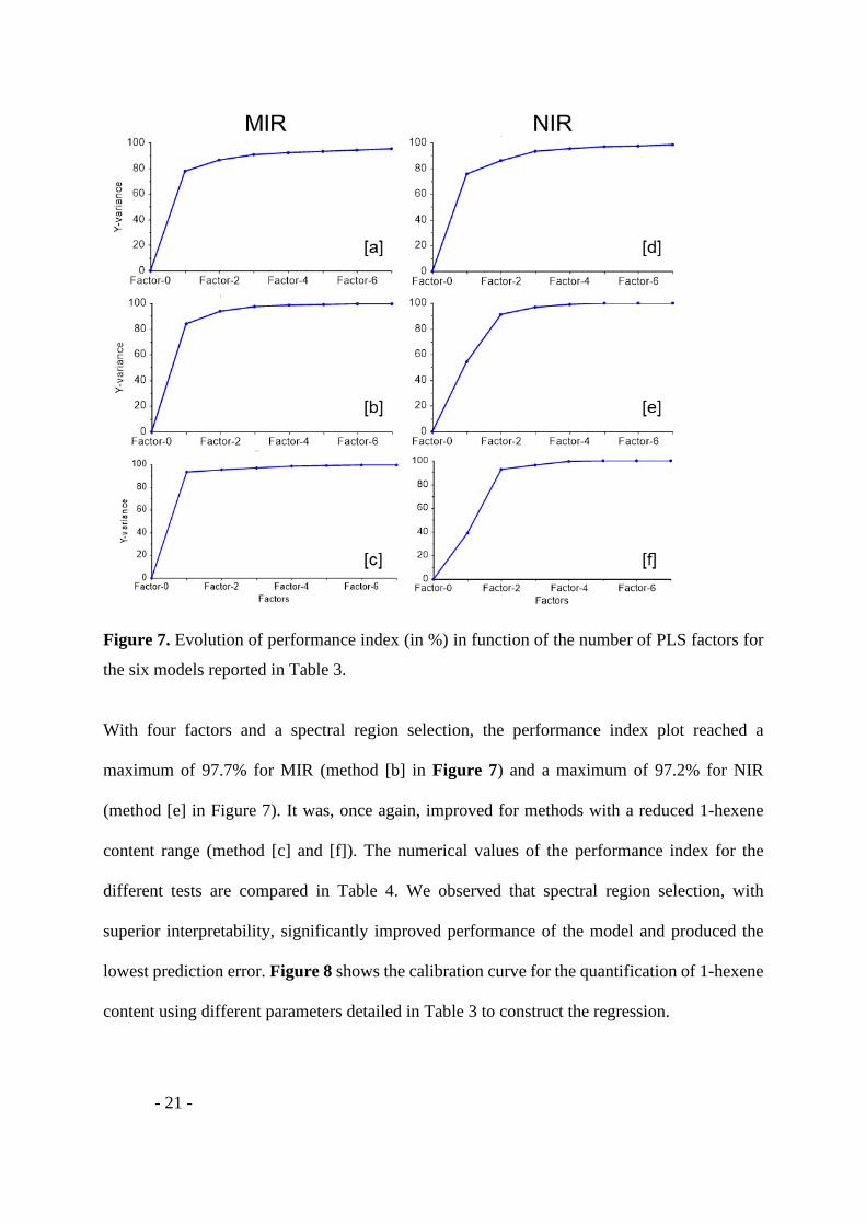
Figure 7. Evolution of performance index (in %) in function of the number of PLS factors for

the six models reported in Table 3.

With four factors and a spectral region selection, the performance index plot reached a

maximum of 97.7% for MIR (method [b] in Figure 7) and a maximum of 97.2% for NIR

(method [e] in Figure 7). It was, once again, improved for methods with a reduced 1-hexene

content range (method [c] and [f]). The numerical values of the performance index for the

different tests are compared in Table 4. We observed that spectral region selection, with

superior interpretability, significantly improved performance of the model and produced the

lowest prediction error. Figure 8 shows the calibration curve for the quantification of 1-hexene

content using different parameters detailed in Table 3 to construct the regression.

- 22 -

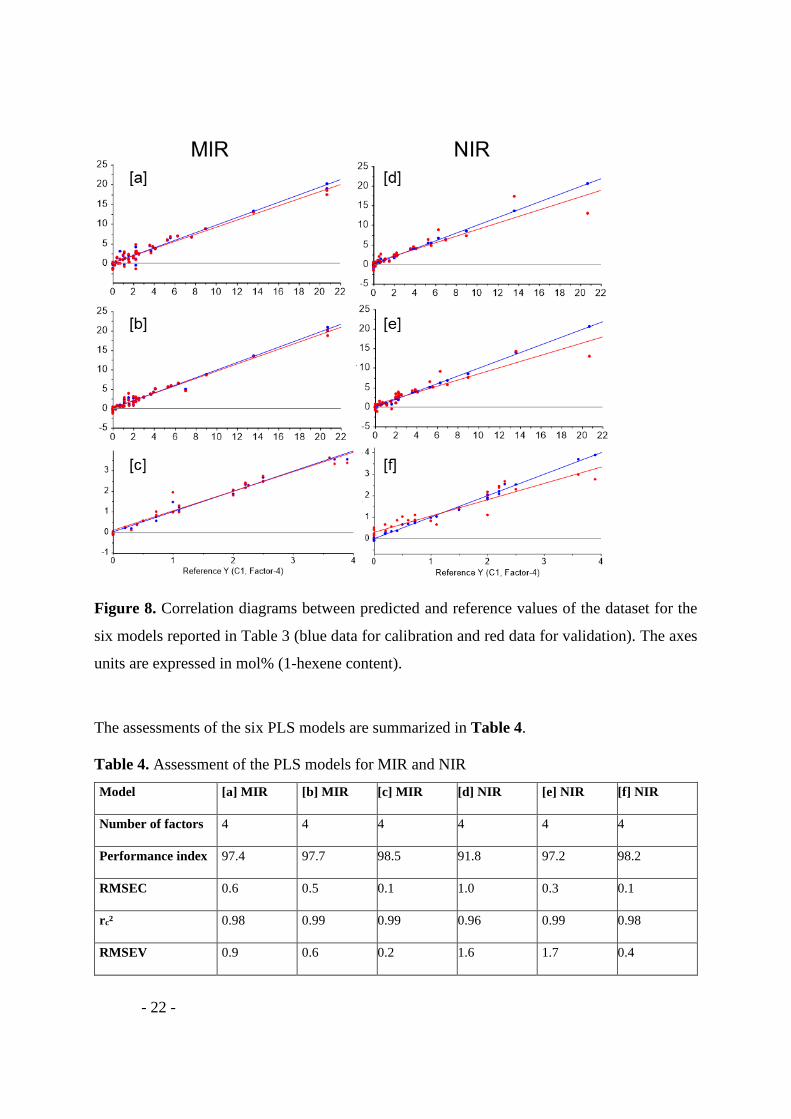
Figure 8. Correlation diagrams between predicted and reference values of the dataset for the

six models reported in Table 3 (blue data for calibration and red data for validation). The axes

units are expressed in mol% (1-hexene content).

The assessments of the six PLS models are summarized in Table 4.

Table 4. Assessment of the PLS models for MIR and NIR

Model [a] MIR [b] MIR [c] MIR [d] NIR [e] NIR [f] NIR

Number of factors 4 4 4 4 4 4

Performance index 97.4 97.7 98.5 91.8 97.2 98.2

RMSEC 0.6 0.5 0.1 1.0 0.3 0.1

rc² 0.98 0.99 0.99 0.96 0.99 0.98

RMSEV 0.9 0.6 0.2 1.6 1.7 0.4

- 23 -

rv² 0.97 0.98 0.97 0.86 0.85 0.84

The RMSEV values for the MIR model were slightly better than that values of NIR model.

Finally, it appears that the methods [b] and [e] were reliable for the determination of the 1-

hexene content in copolymers containing high co-monomer content (up to 21 mol%). For lower

content the methods [c] and [f] will be the most efficient and suitable. The repeatability and the

validity of both methods were evaluated using new samples.

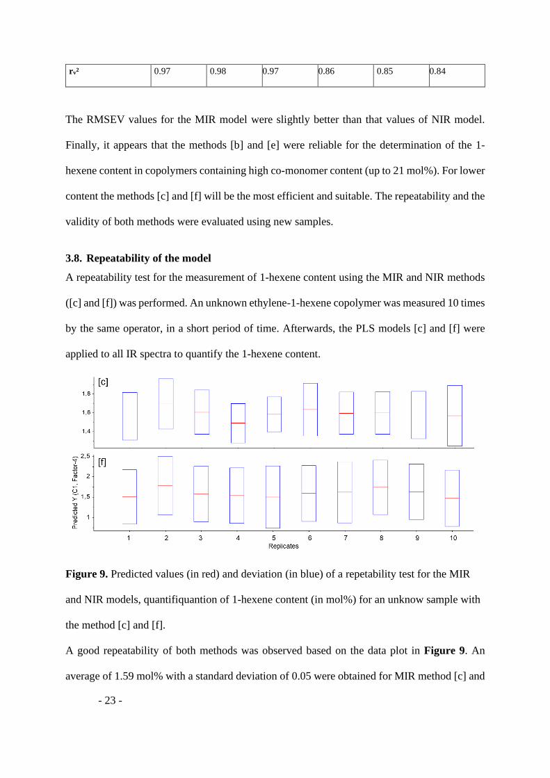
3.8. Repeatability of the model

A repeatability test for the measurement of 1-hexene content using the MIR and NIR methods

([c] and [f]) was performed. An unknown ethylene-1-hexene copolymer was measured 10 times

by the same operator, in a short period of time. Afterwards, the PLS models [c] and [f] were

applied to all IR spectra to quantify the 1-hexene content.

Figure 9. Predicted values (in red) and deviation (in blue) of a repetability test for the MIR

and NIR models, quantifiquantion of 1-hexene content (in mol%) for an unknow sample with

the method [c] and [f].

A good repeatability of both methods was observed based on the data plot in Figure 9. An

average of 1.59 mol% with a standard deviation of 0.05 were obtained for MIR method [c] and

- 24 -

an average of 1.60 mol% and standard deviation of 0.08 were obtained for NIR method [f].

Since a very similar average value for both methods and low sigma values were obtained, we

concluded that the proposed models were accurate. Furthermore, the values were in good

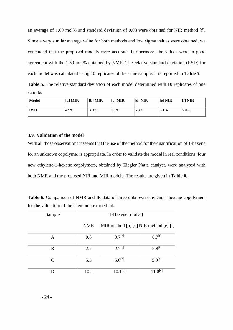
agreement with the 1.50 mol% obtained by NMR. The relative standard deviation (RSD) for

each model was calculated using 10 replicates of the same sample. It is reported in Table 5.

Table 5. The relative standard deviation of each model determined with 10 replicates of one

sample.

Model [a] MIR [b] MIR [c] MIR [d] NIR [e] NIR [f] NIR

RSD 4.9% 3.9% 3.1% 6.8% 6.1% 5.0%

3.9. Validation of the model

With all those observations it seems that the use of the method for the quantification of 1-hexene

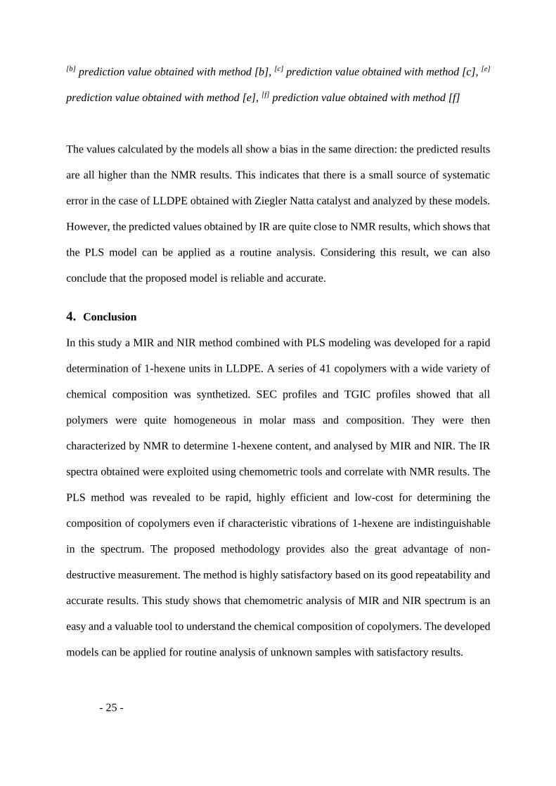
for an unknown copolymer is appropriate. In order to validate the model in real conditions, four

new ethylene-1-hexene copolymers, obtained by Ziegler Natta catalyst, were analysed with

both NMR and the proposed NIR and MIR models. The results are given in Table 6.

Table 6. Comparison of NMR and IR data of three unknown ethylene-1-hexene copolymers

for the validation of the chemometric method.

Sample 1-Hexene [mol%]

NMR MIR method [b] [c] NIR method [e] [f]

A 0.6 0.7[c] 0.7[f]

B 2.2 2.7[c] 2.8[f]

C 5.3 5.6[b] 5.9[e]

D 10.2 10.1[b] 11.0[e]

- 25 -

[b] prediction value obtained with method [b], [c] prediction value obtained with method [c], [e]

prediction value obtained with method [e], [f] prediction value obtained with method [f]

The values calculated by the models all show a bias in the same direction: the predicted results

are all higher than the NMR results. This indicates that there is a small source of systematic

error in the case of LLDPE obtained with Ziegler Natta catalyst and analyzed by these models.

However, the predicted values obtained by IR are quite close to NMR results, which shows that

the PLS model can be applied as a routine analysis. Considering this result, we can also

conclude that the proposed model is reliable and accurate.

4. Conclusion

In this study a MIR and NIR method combined with PLS modeling was developed for a rapid

determination of 1-hexene units in LLDPE. A series of 41 copolymers with a wide variety of

chemical composition was synthetized. SEC profiles and TGIC profiles showed that all

polymers were quite homogeneous in molar mass and composition. They were then

characterized by NMR to determine 1-hexene content, and analysed by MIR and NIR. The IR

spectra obtained were exploited using chemometric tools and correlate with NMR results. The

PLS method was revealed to be rapid, highly efficient and low-cost for determining the

composition of copolymers even if characteristic vibrations of 1-hexene are indistinguishable

in the spectrum. The proposed methodology provides also the great advantage of non-

destructive measurement. The method is highly satisfactory based on its good repeatability and

accurate results. This study shows that chemometric analysis of MIR and NIR spectrum is an

easy and a valuable tool to understand the chemical composition of copolymers. The developed

models can be applied for routine analysis of unknown samples with satisfactory results.

- 26 -

Acknowledgments: the authors thank the NMR Polymer Center of Institut de Chimie de Lyon

(FR5223) for assistance and access to the NMR facilities and Stephane Lebras from Thermo

Fisher Scientific for support in IR.

Keywords: infrared; near infrared; ethylene-1-hexene copolymer; LLDPE; chemometrics

Table of Contents

The comonomer content has a strong impact on the properties of LLDPEs. This article

describes a rapid investigation method, based on a combination of mid and near infrared

spectroscopy and chemometrics tools, for measuring the amount of comonomers. The

processing and the assessment of the obtained regression models are discussed and show that

the methods are efficient, accurate and fast.

- 27 -

- 28 -

[1] R. Mulhaupt, Macromol. Chem. Phys. 2003, 204, 289.

[2] W. D. Sauter, M. Taoufik, C. Boisson, Polymers 2017, 9.

[3] M. M. Stalzer, M. Delferro, T. J. Marks, Catal. Lett. 2015, 145, 3.

[4] M. P. McDaniel, Adv. Catal. 2010, 53, 123.

[5] V. Kumar, C. R. Locker, P. J. in ’t Veld, G. C. Rutledge, Macromolecules 2017, 50, 1206.

[6] S. Bensason, J. Minick, A. Moet, S. Chum, A. Hiltner, E. Baer, J. Polym. Sci. Pol. Phys.

1996, 34, 1301.

[7] J. P. Blitz, D. C. McFaddin, J. Appl. Polym. Sci. 1994, 51, 13.

[8] L. H. Cross, R. B. Richards, H. A. Willis, Faraday Discuss. 1950, 9, 235.

[9] T. Usami, S. Takayama, Polym. J. 1984, 16, 731.

[10] C. France, P. J. Hendra, W. F. Maddams, H. A. Willis, Polymer 1987, 28, 710.

[11] J. C. Randall, J. Polym. Sci. Pol. Phys. 1973, 11, 275.

[12] D. E. Dorman, E. P. Otocka, F. A. Bovey, Macromolecules 1972, 5, 574.

[13] W. Liu, P. L. Rinaldi, L. H. McIntosh, R. P. Quirk, Macromolecules 2001, 34, 4757.

[14] M. E. A. Cudby, A. Bunn, Polymer 1976, 17, 345.

[15] L. Wild, T. R. Ryle, D. C. Knobeloch, I. R. Peat, J. Polym. Sci. Pol. Phys. 1982, 20, 441.

[16] L. Wild, Adv. Polym. Sci. 1991, 98, 1.

[17] L. Wild, C. Blatz, New Adv. Polyolefins, Plenum Press, New York, 1993.

[18] E. Cossoul, L. Baverel, E. Martigny, T. Macko, C. Boisson, O. Boyron, Macromol. Symp.

2013, 330, 42.

[19] T. Macko, H. Pasch, Macromolecules 2009, 42, 6063.

[20] B. Monrabal, J. Blanco, J. Nieto, J. B. P. Soares, J. Polym. Sci. Pol. Chem. 1999, 37, 89.

[21] J. B. P. Soares, S. Anantawaraskul, J. Polym. Sci. Pol. Phys. 2005, 43, 1557.

[22] T. Macko, R. Bruell, Y. Zhu, Y. Wang, J. Sep. Sci. 2010, 33, 3446.

- 29 -

[23] B. Monrabal, L. Romero, Macromol. Chem. Phys. 2014, 215, 1818.

[24] R. Cong, W. de Groot, A. Parrott, W. Yau, L. Hazlitt, R. Brown, M. Miller, Z. Zhou,

Macromolecules (Washington, DC, U. S.) 2011, 44, 3062.

[25] B. Monrabal, Adv. Polym. Sci. 2013, 257, 203.

[26] R. Chitta, T. Macko, R. Bruell, C. Boisson, E. Cossoul, O. Boyron, Macromol. Chem.

Phys. 2015, 216, 721.

[27] F. Brunel, O. Boyron, A. Clement, C. Boisson, Macromol. Chem. Phys. 2019, 220,

1800496.

[28] E. Roumeli, A. Markoulis, T. Kyratsi, D. Bikiaris, K. Chrissafis, Polym. Degrad. Stabil.

2014, 100, 42.

[29] T. Usami, Y. Gotoh, S. Takayama, H. Ohtani, S. Tsuge, Macromolecules 1987, 20, 1557.

[30] S. Duc, N. Lopez, Polymer 1999, 40, 6723.

[31] O. Boyron, T. Marre, A. Delauzun, R. Cozic, C. Boisson, Macromol. Chem. Phys. 2019,

1900162.

[32] J. L. Koenig, M. K. Antoon, Appl. Opt. 1978, 17, 1374.

[33] C. Baker, P. David, W. F. Maddams, Makromol. Chem. 1979, 180, 975.

[34] J. B. Huang, J. W. Hong, M. W. Urban, Polymer 1992, 33, 5173.

[35] F. M. Mirabella, Appl. Spectrosc. Rev. 1985, 21, 45.

[36] K. Sahre, U. Schulze, K.-J. Eichhorn, B. Voit, Macromol. Chem. Phys. 2007, 208, 1265.

[37] A. Cherfi, G. Févotte, Macromol. Chem. Phys. 2002, 203, 1188.

[38] M. P. B. Van Uum, H. Lammers, J. P. De Kleijn, Macromol. Chem. Phys. 1995, 196, 2023.

[39] L. M. Santos, M. J. Amaral, C. Dariva, E. Franceschi, A. F. Santos, O. Boyron, T. F. L.

McKenna, Macromol. React. Eng. 2017, 11, 1700007.

[40] E. Caro, E. Comas, Talanta 2017, 163, 48.

[41] M. A. McRae, W. F. Maddams, Makromol. Chem. 1976, 177, 449.

- 30 -

[42] K. Sano, M. Shimoyama, M. Ohgane, H. Higashiyama, M. Watari, M. Tomo, T. Ninomiya,

Y. Ozaki, Appl. Spectrosc. 1999, 53, 551.

[43] M. Shimoyama, T. Ninomiya, K. Sano, Y. Ozaki, H. Higashiyama, M. Watari, and M.

Tomo, J. Near Infrared Spectrosc. 1998, 6, 317.

[44] R. W. Gerlach, B. R. Kowalski, H. O. A. Wold, Anal. Chim. Acta 1979, 112, 417.

[45] P. Bastien, V. E. Vinzi, M. Tenenhaus, Comput. Stat. Data Anal. 2005, 48, 17.

[46] B. S. Dayal, J. F. MacGregor, J. Chemometr. 1997, 11, 73.

[47] F. Lindgren, P. Geladi, S. Wold, J. Chemometr. 1993, 7, 45.

[48] S. Rännar, F. Lindgren, P. Geladi, S. Wold, J. Chemometr. 1994, 8, 111.

[49] O. Boyron, B. MacQueron, M. Taam, J. Thuilliez, C. Boisson, Macromol. Chem. Phys.

2018, 219, 1700609.

[50] W. Kaminsky, Macromolecules 2012, 45, 3289.

[51] W. Kaminsky, A. Funck, H. Hähnsen, Dalton Trans. 2009, 41, 8803.

[52] H. Sinn, W. Kaminsky, H.-J. Vollmer, R. Woldt, Angew. Chem. Int. Ed. 1980, 19, 390.

[53] F. Prades, J.-P. Broyer, I. Belaid, O. Boyron, O. Miserque, R. Spitz, C. Boisson, Acs

Catalysis 2013, 3, 2288.

[54] J. C. Randall, J. Macromol. Sci. Polymer Rev 1989, 29, 201.

[55] N. Inwong, S. Anantawaraskul, J. B. P. Soares, A. Z. Al- Khazaal, Macromol. Symp. 2015,

356, 54.

[56] B. Monrabal, N. Mayo, R. Cong, Macromol. Symp. 2012, 312, 115.

[57] A. Z. Al-Khazaal, J. B. P. Soares, Macromol. Chem. Phys. 2014, 215, 465.

[58] A. Alghyamah, J. B. P. Soares, Ind. Eng. Chem. Res. 2014, 53, 9228.

[59] F. M. Rugg, J. J. Smith, L. H. Wartman, J. Polym. Sci. 1953, 11, 1.

[60] A. H. Willbourn, J. Polym. Sci. 1959, 34, 569.

[61] S. Krimm, C. Y. Liang, G. B. B. M. Sutherland, J. Chem. Phys. 1956, 25, 549.

- 31 -

[62] K. Rossmann, J. Chem. Phys. 1955, 23, 1355.

[63] M. Mizushima, T. Kawamura, K. Takahashi, K.-h. Nitta, Polym. J. 2011, 44, 162.

[64] S. Watanabe, J. Dybal, K. Tashiro, Y. Ozaki, Polymer 2006, 47, 2010.

[65] A. Höskuldsson, J. Chemometr. 1988, 2, 211.

[66] J. Luo, K. Ying, J. Bai, Signal Process. 2005, 85, 1429.

[67] A. Savitzky, M. J. E. Golay, Anal. Chem. 1964, 36, 1627.

[68] P. A. Gorry, Anal. Chem. 1990, 62, 570.