Embed Size (px)
Citation preview
5620 | Chem. Soc. Rev., 2017, 46, 5620--5646 This journal is©The Royal Society of Chemistry 2017
Cite this: Chem. Soc. Rev., 2017,
46, 5620
Two-dimensional flow of driven particles:a microfluidic pathway to the non-equilibriumfrontier
Tsevi Beatus,a Itamar Shani,b Roy H. Bar-Ziv*c and Tsvi Tlusty *def
We discuss the basic physics of the flow of micron-scale droplets in 2D geometry. Our focus is on the
use of droplet ensembles to look into fundamental questions of non-equilibrium systems, such as the
emergence of dynamic patterns and irreversibility. We review recent research in these directions, which
demonstrate that 2D microfluidics is uniquely set to study complex out-of-equilibrium phenomena
thanks to the simplicity of the underlying Stokes flow and the accessibility of lab-on-chip technology.
1 Microfluidics and the challenges ofnon-equilibrium systems
When a system is kicked out of equilibrium it leaves the safezone of classical thermodynamics into a realm where the rulesof the game are still very blurry. While at equilibrium we have atour disposal powerful symmetries and extremum principles,such as the equipartition of energy and maximum entropy, thetoolbox of nonequilibrium physics is much smaller. Recent pro-gress has brought several fluctuation theorems and identities,but general principles like the ones of equilibrium systems arestill lacking.1–3
The presence of long-range forces makes out-of-equilibriumsystems even harder to understand. Such forces, like gravity forexample, decay like a power law 1/ra with an exponent smalleror equal to the dimension of the system, a r d. Long-rangeforces render the system strongly-interacting. Namely, nomatter what size the system is, all particles are coupled. In otherwords, one cannot break such a system into small decoupledsubsystems. This inability is called non-additivity because, dueto the long-range forces, one cannot calculate basic quantitiessuch as the overall interaction energy simply by adding upthe energies of all subsystems. As a result, non-additive,
strongly-interacting systems behave quite differently even atequilibrium, and cannot be treated with the standard tools ofstatistical mechanics.4
Two of the fundamental forces of nature, gravity and electro-dynamics are manifested by long-range interactions that decaylike 1/r. Other, effective interactions, like the forces in a stressedelastic medium or in a dipolar fluid, are also long-range. It thereforecomes as no surprise that non-equilibrium systems with long-range interactions are abundant in Nature. Still, despite theiromnipresence, their governing principles are far from beingfully understood. In particular, the general principles by whichlong-range forces give rise to the observed collective modes anddynamical patterns is a basic open question.5
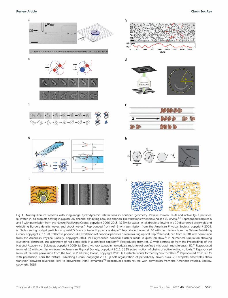
When general principles are yet to be found, simple non-equilibrium systems where one can be playful and search forunderstanding are most valuable. Long-range forces would bea bonus, a double challenge in one experiment. Fig. 1 depictsseveral experiments where particles flow far from equilibriumin a low-dimensional geometry and are governed by long-rangehydrodynamic interactions, including: phonons in a 1D micro-fluidic crystal,6,7 Burgers shock waves in a 2D microfluidicdroplets ensemble,8 self-steering of particles in confined flowcontrolled by particle shape,9 collective excitations of hydro-dynamically coupled driven colloidal particles,10 colloidal clustersmade in quasi-2D flow,11 clustering and alignment of vesiclesand red blood cells in confined channels,12 density shock wavesin confined micro-swimmers,13 directed motion in populationsof motile colloids,14 unstable fronts and motile structures formedby microrollers,15 and periodically driven quasi-2D dropletsensembles.98
As a generic example for non-equilibrium systems with long-range interactions, this mini-review focuses on ensembles ofmicron-scale droplets driven by flow in a quasi-2D channel. Thereview first demonstrates the underlying physical principles of
a The Rachel and Selim Benin School of Computer Science and Engineering,
The Alexander Grass Center for Bioengineering, and The Silberman Institute of
Life Science, The Hebrew University of Jerusalem, Israelb Institute for Research in Electronics and Applied Physics, University of Maryland,
College Park, MD, USAc Dept. of Materials and Interfaces, Weizmann Institute of Science, Rehovot, Israel.
E-mail: [email protected] Center for Soft and Living Matter, Institute for Basic Science (IBS), Ulsan, Koreae Dept. of Physics, Ulsan National Institute of Science and Technology, Ulsan, Koreaf Simons Center for Systems Biology, Institute for Advanced Study, Princeton, NJ,
USA. E-mail: [email protected]
Received 24th May 2017
DOI: 10.1039/c7cs00374a
rsc.li/chem-soc-rev
Chem Soc Rev
REVIEW ARTICLE
This journal is©The Royal Society of Chemistry 2017 Chem. Soc. Rev., 2017, 46, 5620--5646 | 5621
Fig. 1 Nonequilibrium systems with long-range hydrodynamic interactions in confined geometry. Passive (driven) (a–f) and active (g–i) particles.(a) Water-in-oil droplets flowing in a quasi-2D channel exhibiting acoustic phonon-like vibrations when flowing as a 1D crystal.6,7 Reproduced from ref. 6and 7 with permission from the Nature Publishing Group, copyright 2006, 2015. (b) Similar water-in-oil droplets flowing in a 2D disordered ensemble andexhibiting Burgers density waves and shock waves.8 Reproduced from ref. 8 with permission from the American Physical Society, copyright 2009.(c) Self-steering of rigid particles in quasi-2D flow controlled by particle shape.9 Reproduced from ref. 86 with permission from the Nature PublishingGroup, copyright 2013. (d) Collective phonon-like excitations of colloidal particles driven in a ring optical trap.10 Reproduced from ref. 10 with permissionfrom the American Physical Society, copyright 2014. (e) Polymerized colloidal clusters made in quasi-2D flow.11 (f) Numerical simulation showingclustering, distortion, and alignment of red blood cells in a confined capillary.12 Reproduced from ref. 12 with permission from the Proceedings of theNational Academy of Sciences, copyright 2009. (g) Density shock waves in numerical simulation of confined microswimmers in quasi-2D.13 Reproducedfrom ref. 13 with permission from the American Physical Society, copyright 2016. (h) Directed motion of chains of active, rolling colloids.14 Reproducedfrom ref. 14 with permission from the Nature Publishing Group, copyright 2013. (i) Unstable fronts formed by ‘microrollers’.15 Reproduced from ref. 15with permission from the Nature Publishing Group, copyright 2016. (j) Self organization of periodically driven quasi-2D droplets ensembles showtransition between reversible (left) to irreversible (right) dynamics.98 Reproduced from ref. 98 with permission from the American Physical Society,copyright 2015.
Review Article Chem Soc Rev
5622 | Chem. Soc. Rev., 2017, 46, 5620--5646 This journal is©The Royal Society of Chemistry 2017
this system, and then summarizes the relevant literature (Section 5).While large-scale collective modes are common to both, driven andactive particles differ in several basic aspects: driven particles movein the direction of the driving field, whereas active particles maychange the direction of self-propulsion. In addition, active particlesare often subject to a force dipole – in contrast to the forcemonopole acting on a driven particles – which changes thesymmetry of hydrodynamic field they induce.
In Section 2, we review the physics of microfluidic dropletensembles and explain how 2D flows are an excellent toy modelfor studying strongly-coupled non-equilibrium systems. Thisflow gives rise to rich many-body phenomena owing to long-rangeforces that scale like 1/r2. Yet, unlike other strongly-coupledsystems, the flow is tractable, thanks to the combination of lowdimensionality and linear hydrodynamic equations. Theoretically,the microfluidic Stokes flow is described in terms of an effective2D potential flow, which is simple to solve. More importantly, theresulting forces are described by 2D dipoles that decay as 1/r2. Wewill explain that in this marginal case – where the dimension ofthe system d is equal to the power of the interaction, a = d = 2 – thecoupling is strong but the divergence is weak, i.e. logarithmic.Experimentally, the geometry of the microfluidic channel and itstypical spatial and temporal scales, render the flow easy tomeasure with standard optical microscopy. Altogether, thetheoretical and experimental accessibility set driven microfluidicdroplets as an ideal system for studying non-equilibrium physics,as we demonstrate in the next section.
In Section 3, we explore how, by simple analysis of thedynamic equations and careful examination of experimentaldata, one can discover the basic collective modes and understandhow they emerge from the elementary interactions. These modesinclude phonon-like vibrations, non-linear shock waves and long-range orientational order. In Section 4, we give a do-it-yourselfmanual for constructing the experimental setup and performingthe basic measurements.
In the concluding Section 5, we argue that what has beenrevealed so far merely touched the surface of a deep sea of non-equilibrium physics, which can be explored by observingmicrofluidic droplet flow. The close link between theory andexperiment provides a unique pathway into non-equilibriumsystems. In particular, it is an ideal system for looking at thegeometric interplay among long-range forces, boundaries,shape and symmetry. The main purpose of this short reviewis to introduce the necessary physics and engineering know-how, on an intuitive and practical level, such that anyone maychoose their own path in this microfluidic sea.
2 The physics of 2D microfluidicdroplet ensembles2.1 Making micro-pancakes in the lab
With the success of microfluidics, lab-on-chip devices are now astaple in many labs. In particular, devices in which micron-sizeparticles are generated and manipulated became accessible.We have at our hand sophisticated devices that can produce,
process, and measure thousands of micro-droplets per second.For surveys of microfluidic engineering and applications acurious reader may check the reviews.16–25 That said, the kindof devices one would need for studying non-equilibrium physicsare more modest and can be built in a lightly-equipped lab aftershort training.
The basic setup that led to many of the observationsdescribed in this review is shown in Fig. 1a. It is a T-junctionwhere an oil stream is pinching a water stream into a uniformtrain of small droplets.19,26,27 More details and technical know-how will be given in Section 4, but first let us get a basic pictureof what happens at the junction: water and oil streams arepushed by pressure into the junction. When a water ‘‘finger’’protrudes into the junction, it is subject to the stress by theoil flowing in the remaining unblocked channel and slightlyupstream. An interplay between the hydrodynamic stress andsurface tension at the oil–water interface ends when a waterdroplet is pinched off and carried downstream by the oil. Then thewater finger recedes and the droplet formation cycle is reiterated.27
The almost-exact periodicity of the formation process ensures thatthe droplets are practically monodispersed and equally spaced.One can tune both the size of the droplets and their formation rateby varying the input pressure of the oil and water streams and thegeometry of the T-junction. It is also possible to exchange thefluids and use the T-junction to make oil-in-water droplets, whiletaking care of the wetting properties of the channel inner surface:one must set the channel boundary hydrophobic for water-in-oildroplets and hydrophilic for oil-in-water droplets. If the fluidconsisting the droplets wets the surface, droplets will tend to stickto the channel.
When the volume pinched off at the T-junction is small, thenewly formed droplet is spherical, with diameter smaller thanthe channel height h, 2Rsph o h. Such small droplets are carriedaway at approximately the velocity of the surrounding oil stream.However, for our purpose of looking at strongly interactingparticles, we will see that it is preferable to make larger droplets.If these droplets were spherical, their diameter would havebeen larger than the channel height, 2Rsph 4 h. So to fit intothe channel, the droplets must squeeze between the floor andceiling and take the form of disc-like ‘pancakes’ with radiusR 4 Rsph 4 h/2. As long as the droplets radius is small enough,surface tension preserves their disc-like shape against distor-tions by shear forces. In the experiments described below,droplets maintained circular shape in the xy plane withinmeasurement accuracy.
Importantly, touching the channel floor and ceiling inducessignificant friction. Unlike small spherical droplets, the frictionsignificantly slows down the micro-pancakes and they lagbehind the oil stream. Typically, the droplets are much slowerthan the oil, and are carried at a velocity ud, which is 3–4 timesslower than the velocity of the surrounding oil, uN
oil.
2.2 Microfluidic flow is viscous and linear
A moving fluid carries momentum. Just like heat, there are two waysto transport momentum. One is inertial convection: displacinga fluid element also transports its momentum. The second is
Chem Soc Rev Review Article
This journal is©The Royal Society of Chemistry 2017 Chem. Soc. Rev., 2017, 46, 5620--5646 | 5623
the diffusion of momentum between fluid elements by viscousforces. The significance of inertial convection relative to viscousdiffusion of momentum can be expressed in terms of their ratio.It yields a dimensionless quantity called the Reynolds number,Re: a small Re value implies viscous flow, whereas large valuesoccur in turbulent flows (and other laminar, high-Re flows). TheReynolds number is determined by the typical scales of length,velocity, density and viscosity of the system
Re ¼ momentum convection
momentum diffusion¼ ½length�½velcoity�½density�½viscosity� :
For a microfluidic droplet (Fig. 1a), the typical experimentalscales give a Reynolds number of the order Re = RuN
oilr0/Zo B10�4–10�3, in which r0 is the oil density, and Zo is its viscosity.As one intuitively expects, owing to its small length-scale, themicrofluidic flow is well within the viscous regime, Re { 1,where inertia is negligible. For the same reason, the motion ofmicroorganisms also lies in this regime.28
In the low-Reynolds limit, the nonlinear Navier–Stokes hydro-dynamic equations take a simple form, known as the Stokesequation,
Zor2v = rP (1)
where v(r) is the oil velocity at r and P(r) is the local pressure.To solve for the flow, one also needs to mathematically expressthe continuity and incompressibility of the flow as
r�v = 0. (2)
The hallmark of the hydrodynamic eqn (1) and (2) is theirlinearity. This simplicity of the equations has several implica-tions29 that will prove important to 2D microfluidic flow:
(P1) Uniqueness: for given geometry and boundary conditions(BC), one unique solution exists for the velocity and pressurefields, v(r) and P(r) (unlike turbulent flow that may have multiplesolutions).
(P2) Reversibility: by reversing the pressure gradientrP - �rP, the direction of the flow reverses v(r)- �v(r),and one obtains time-reversed flow where the fluid looks like ina backwards played movie.
(P3) Superposition: one may change the BC (for example bymoving a droplet at a different velocity or moving a previouslystatic wall) and the solution will accommodate the change byaltering the flow field. One can then obtain another solution bylinear combination of the solutions and the BC, l1v1(r) + l2v2(r)and l1P1(r) + l2P2(r).
(P4) No explicit time dependence: time does not appear expli-citly in the Stokes eqn (1). By scaling the velocity and pressure by afactor l, one obtains exactly the same streamlines, only with fluxesscaled by the same factor. The flow rate is determined by the BC,since the physical parameters themselves cannot define a time-scale. This implies instantaneity: the Stokes flow is determined bythe BC without knowledge of the flow at previous times.†
It is natural to ask at this point: if Stokes flow is so linearand simple, where do all the non-linear phenomena we discussin this review come from? – the answer is that non-linearitycomes from the boundaries. In our system these are theboundaries of the moving pancake-like droplets. Indeed, theoil flow between the droplets’ boundaries is the solution oflinear equations. But the forces that they exert on each other asa result are highly non-linear.
This property is a major advantage of looking at Stokes flow:to understand and solve it, there is no need to calculate theintricate streamlines. Instead, it is enough to sum up the effectiveinteractions. In our system of choice, 2D microfluidic droplets,we will see that each droplet is equivalent to a hydrodynamicdipole. The collective motion of an ensemble of such droplets,can be predicted by calculating the dynamics of interactingdipoles without the need to invoke explicitly the hydrodynamicflows. This is thanks to the linearity of the Stokes flow thatallows us to account for the flow via the effective interaction ofthe boundaries.
2.3 The 2D microfluidic flow is described by a potential
To see how the slowness of the pancake-like droplets gives riseto long-range hydrodynamic interactions, we solve the Stokesflow for a droplet dragged in a channel by the oil stream. Wedescribe the main features of the solution in the following, whilea more detailed explanation is given in Beatus et al.31 The dropletis moving at a velocity ud with respect to the channel (Fig. 1a),which is much slower than the oil velocity far from the droplet,uN
oil 4 ud. The motion is in the x-direction in a channel whosefloor and ceiling are in the z = �h/2 planes.
The geometry of the channel is that of a thin sheet of fluid.The horizontal x and y dimensions are much larger than thevertical z dimension of the channel height h, which is typicallyB10–100 mm. This separation of scales in this ‘quasi-2D’ geometrysignificantly simplifies the problem: as long as our interest is inlength scales much larger than h, we can decompose the velocityfield into v(x,y,z) = uoil(x,y) f (z), such that f (z) = (3/2)[1 � (2z/h)2]is a parabolic Poiseuille profile, and uoil(x,y) is the velocity inthe xy plane averaged along the z-axis.
Thanks to the separation of scales, called sometimesthe ‘lubrication approximation’,29 the Stokes eqn (1) and theincompressibility condition (2), take a particularly simple formof a potential equation:
uoil(x,y) = rf, (3)
r2f = 0. (4)
The velocity in this 2D Laplace equation is the gradient of aneffective potential, f(x,y) � (�h2/12Zo)P. Potential flows in 2Dare particularly easy to solve because they can be described byanalytic functions of a complex variable.30,31
2.4 2D droplets induce hydrodynamic dipoles
In the absence of droplets, the stream lines in the channel arestraight lines in the direction of the pressure gradient. But theoil flux cannot penetrate the circumference of the droplet.
† Incompressible potential flow is also instantaneous since it is governed by theLaplace equation, which does not depend on time explicitly. As in Stokes flow,time enters only through the boundary conditions.29,30
Review Article Chem Soc Rev
5624 | Chem. Soc. Rev., 2017, 46, 5620--5646 This journal is©The Royal Society of Chemistry 2017
Therefore, if the water droplet is slower than the oil, thestreamlines have to curve around it. The corresponding boundarycondition for the flow at the water–oil interface is of vanishingvelocity in the perpendicular to the droplet edge (slip boundarycondition).
Solving the Laplace eqn (3) and (4) with the slip boundarycondition at the droplet’s edge, we find that the perturbation ofthe uniform flow describes a 2D hydrodynamic dipole,
fdðrÞ ¼ d0 �cos yr: (5)
The magnitude of the dipole d0 is proportional to velocity lagdu between the droplet and the unperturbed oil,
d0 = du�R2 = (uN
oil � ud)R2. (6)
A similar hydrodynamic dipole also describes the flow fieldaround a Brownian particle confined in quasi-2D.32 However, incontrast to the dipole of a microfluidic droplet, which isparallel to the external driving flow field, the dipole of theBrownian particle points in the direction of the instantaneousthermal velocity.
The potential flow eqn (3) asserts that the dipolar velocityfield is the gradient of the potential (5), ud = rfd(r). Thevelocity in the x and y directions is,
ud;xðrÞ ¼ �d0
r2� cos 2y;
ud;yðrÞ ¼ �d0
r2� sin 2y:
(7)
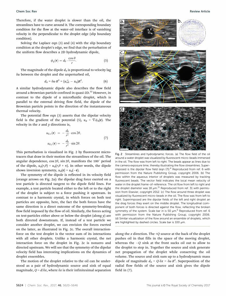
This perturbation is visualized in Fig. 2 by fluorescent micro-tracers that draw in their motion the streamlines of the oil. Theangular dependence, cos 2y, sin 2y, manifests the 1801 periodof the dipole, ud(r,y) = ud(r,y + p). In other words, the dipoleshows inversion symmetry, ud(r) = ud(�r).
The symmetry of the dipole is reflected in its velocity field(orange arrows on Fig. 2a): the dipolar drag force exerted on atest particle is directed tangent to the dipole field lines. Forexample, a test particle located either to the left or to the rightof the droplet is subject to a force pushing it upstream. Incontrast to a harmonic crystal, in which forces on both testparticles are opposite, here, the fact the both forces have thesame direction is a direct outcome of the symmetry-breakingflow field imposed by the flow of oil. Similarly, the forces actingon test-particles either above or below the droplet (along y) areboth directed downstream. If, instead of a test particle weconsider another droplet, we can envision the forces exertedon the latter, as illustrated in Fig. 2c. The overall interaction-force on the test droplet is the vector sum of its interactionswith all other droplets. Unlike a harmonic crystal, the netinteraction force on the droplet in Fig. 2c is nonzero anddirected upstream. We will see that the symmetry of the dipolarvelocity field has interesting implications on the dynamics ofdroplet ensembles.
The motion of the droplet relative to the oil can be under-stood as a pair of hydrodynamic source and sink of equalmagnitude, Q = d/dx, where dx is their infinitesimal separation
along the x direction. The +Q source at the back of the dropletpushes oil in that fills in the space of the moving droplet,whereas the �Q sink at the front sucks oil out to allow tothe droplet to step in. Together the source and sink generatenet propagation of the droplet while conserving the oilvolume. The source and sink sum up to a hydrodynamic massdipole of magnitude d0 = Q�dx = du�R2. Superposition of theradial flow fields of the source and sink gives the dipolefield in (7).
Fig. 2 Streamlines and hydrodynamic forces. (a) The flow field of the oilaround a water droplet was visualized by fluorescent micro-beads immersedin the oil. The flow was from left to right. The beads appear as lines due tothe camera exposure time, thereby illustrating the flow streamlines. Super-imposed is the dipolar flow field (eqn (7)).6 Reproduced from ref. 6 withpermission from the Nature Publishing Group, copyright 2006. (b) Theflow within the aqueous interior of droplets was measured by trackingfluorescent beads. The vector field indicates the local mean velocity ofwater in the droplet frame-of-reference. The oil flow from left to right andthe droplet diameter was 18 mm.31 Reproduced from ref. 31 with permis-sion from Elsevier, copyright 2012. (c) The flow around three droplet wasvisualized by fluorescent micro-beads in the oil. The flow was from left toright. Superimposed are the dipolar fields of the left and right droplet anthe drag forces they exert on the middle droplet. The longitudinal com-ponent of both forces is directed against the flow, reflecting the brokensymmetry of the system. Scale bar in is 50 mm.6 Reproduced from ref. 6with permission from the Nature Publishing Group, copyright 2006.(d) Similar visualization of the flow around an ensemble of droplets, whichare highlighted by dashed circles. Scale bar is 100 mm.
Chem Soc Rev Review Article
This journal is©The Royal Society of Chemistry 2017 Chem. Soc. Rev., 2017, 46, 5620--5646 | 5625
2.5 Interplay of friction and drag determines droplet motion
The surrounding oil moves faster than the droplet, and thereforeexerts on it a drag force, Fdrag. This force is the net momentuminflux through the droplet’s surface,30,31
Fdrag ¼1
2xdud þ xd uoil � udð Þ; (8)
with the drag coefficient xd = 24pZoR2/h. The first term in thedrag force (8) describes the force on a droplet carried alongwith the oil (as if du = uoil� ud = 0). The second term is the forcedue to the velocity difference (du a 0).33,34 For example, thedrag on a droplet at rest, ud = 0, is Fdrag = xduoil, while a dropletmoving twice as fast as the oil, ud = 2uoil experiences no force,Fdrag = 0.
The force that opposes the drag is the friction with the floorand ceiling of the channel Ffric, which makes the droplet lagbehind the oil,
Ffric = �mdud, (9)
where md is the friction coefficient. The minus sign indicatesthat friction points in an opposite direction to the droplet’svelocity. The friction force is the outcome of the viscousdissipation of the reticulating inside the droplet,31 as shownin Fig. 2b and c.
Inertia is negligible at the low-Reynolds regime. Therefore,all forces acting on the droplet must balance out (Fig. 2a),Ftotal = Fdrag + Ffric = 0. In the inertial regime, we are used toNewton’s second law, Ftotal = m�du/dt: the acceleration isproportional to the force. Since the net force Ftotal vanishes, itmay seem that all velocities must remain constant. But motionin the viscous regime follows a different logic: the drag Fdrag (8)and friction Ffric (9) forces are proportional to the velocities(Aristotle’s law of motion). So if either of these forces changes,the other force instantaneously counterbalances it by alteringthe velocity. For example, increasing the speed of the driving oilstream by amplifying the oil pressure, leads to a larger dragforce, which would immediately translate into a correspondingincrease of the droplet velocity, and a corresponding increase inthe opposing fiction force.
Since both drag (8) and friction (9) have linear terms in thevelocities, the force balance yields a simple linear relation,
ud = Kuoil. (10)
The speed ratio
K ¼ mdxdþ 1
2
� ��1(11)
depends solely on the geometry of the droplets (R, h) and theviscosities of oil and water (Zo,Zw). Hence, in a monodisperseensemble K is the same for all droplets. The value of the frictioncoefficient md is determined by the viscous dissipation of theeddies inside the water droplet, which is not easy to calculate.However, it is easy to calibrate the speed ratio K and thereby md
by measuring the motion of an isolated droplet and calculatingthe ratio of the velocities, K = ud/uN
oil.
The calibrated value of xd can be used to show that thermaleffects are negligible in the dynamics of the droplet ensemble.We consider an isolated stationary droplet where ud = uoil = 0. Toestimate the thermal effects, we use the Stokes–Einstein relationfor the thermal diffusion coefficient D = kBT/M, in which themobility M relates force and thermal velocity M � F/u. Similarlyto Stokes drag in the case of a sphere in 3D, the droplet’smobility is equivalent to the drag coefficient xd. Using typicalvalues for the droplet ensemble (Table 1), the resulting thermaldiffusion coefficient is D E 10�4 mm2 s�1. This value is 3 ordersof magnitude smaller than the diffusion coefficient of a 1 mmbead in water and, for a moving droplet, the Peclet number isPe � Rud/D E 5 � 107. Hence, thermal effects are negligible andthe droplet dynamics is dominated by the hydrodynamic dipolarinteractions. In a dense ensemble, these interactions, alongwith inter-particle collisions induce seemingly random dropletmotion. These dynamics can be described as effective diffusionwith a coefficient8 Deff E 3 � 102 mm2 s�1, some 5–6 orders ofmagnitude larger than the estimated thermal diffusion.
2.6 Hydrodynamic dipoles exert long-range forces
The force balance eqn (10) implies that, once we calibrated theconstant K, the droplet velocity ud is determined by the localvelocity of the oil uoil. When an ensemble of droplets movesdown a channel, the motion of each droplet induces a long-range 1/r2 dipolar field (7) that perturbs the oil velocity at thepositions of all other droplets (Fig. 2). These velocity perturba-tions induce proportional drag forces (8), and thus constitutean effective dipolar interaction between the droplets.
Droplet pairs are stable. The simplest case of an interactingensemble is that of a pair of droplets35 (Fig. 3). Let us imaginetwo droplets, 1 and 2, driven by a uniform oil flow in a widechannel, far from the walls and any other droplet. An isolateddroplet would have moved at a velocity uiso = KuN
oil (10).Furthermore, let us assume that the two droplets move at thesame velocity, u1 = u2. From the reflection symmetry of (7),it follows that the dipolar field of each droplet at the positionof the other droplet is exactly the same both in magnitude anddirection.
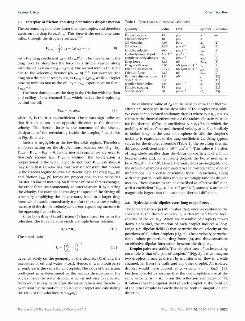
Table 1 Typical values of physical parameters
Quantity Value Unit Symbol Equation
Droplet radius 15 mm R —Channel height 10 mm h —Oil viscosity 0.03 Pa s Zo (1)Oil velocity 1200 mm s�1 uN
oil (6)Droplet velocity 300 mm s�1 uiso (6)Hydrodynamic dipole 2 � 105 mm3 s�1 d0 (6)Dipole velocity along x 36 mm s�1 ud,x (7)Drag force 52.5 nN Fdrag (8)Drag coefficient 0.05 nN (mm s�1)�1 xd (8)Friction coefficient 0.175 nN (mm s�1)�1 md (9)Friction force 52.5 nN Ffric (9)Pairwise dipolar force 1.8 nN f (12)Speed ratio 0.25 — K (11)Dipolar interaction 225 mm s�1 c0 (14)Droplet spacing 75 mm a (21)Sound speed 90 mm s�1 Cs (25)
Review Article Chem Soc Rev
5626 | Chem. Soc. Rev., 2017, 46, 5620--5646 This journal is©The Royal Society of Chemistry 2017
The velocity of a pair of droplets can be found from theequation of motion (10), when we add to the uniform oilvelocity the dipolar interaction,
u1 ¼ Kuoil r1ð Þ ¼ K u1oilxþrf2 r1 � r2ð Þ� �
;
u2 ¼ Kuoil r2ð Þ ¼ K u1oilxþrf1 r2 � r1ð Þ� �
:
Reflection symmetry of the dipole (7) implies rf1(r2 � r1) =rf2(r1 � r2), and therefore u1 = u2. Since the forces that thedroplets exert on each other are equal, the pair is neutrallystable: if the distance or the orientation of the pair change byan external force, the two forces change accordingly but remainequal to each other, keeping the new formation of the pair.
Unless the droplets are very close to each other, their dipolecan be approximated quite well by the dipole field of an isolateddroplet, d0 = (uNoil � uiso)R2 = (1 � K)uNoilR
2 (from eqn (10) and (6)).The actual dipole deviates a bit from d0, but these are higherorder corrections that can be usually disregarded.31,36 Considera pair of droplets at a distance r = |r2 � r1| from each other andorientation y (3). The first-order approximation for the pairvelocity, u1 = u2, is
u1;x ¼ u2;x ¼ uiso � C2ðrÞ cos 2y;
u1;y ¼ u2;y ¼ �C2ðrÞ sin 2y;(12)
where the velocity of an isolated droplet is uiso = KuN
oil. Themagnitude of the two-body dipolar interaction C2(r) is
C2ðrÞ ¼ c0R
r
� �2
; (13)
c0 = K(1 � K)uN
oil, (14)
where c0 is the maximal possible dipolar interaction when thedistance between the droplet is about their size.
The form of this expression captures the underlying physics.The dependence of interaction on the speed ratio, K(1 � K),
indicates the possible physical regimes: It vanishes in the limitof very high friction, md/xd - N, when the droplets hardlymove, K - 0. At the other extreme, of negligible friction,md/xd - 0, the speed ratio is K = 2, and the interaction hasits strongest magnitude, K(1 � K) = �2. One way to reach thisregime of strongly interacting particles is by using gas-filledbubbles instead of liquid-filled droplets, which should dramati-cally reduce friction33 (dissipation in the lubrication layer betweenthe bubble and the channel floor and ceiling might still slow downthe bubble). When the droplets are carried with the oil, K = 1, thereare no dipolar perturbations and hence no interaction. Themaximal positive value of the interaction is obtained for 1
2,where K = 1
4. In the experiments we describe in this reviewK E 0.2–0.4, with K(1 � K) E 0.16–0.24. A list of relevant physicalquantities of the droplets and their interaction is given in Table 1.
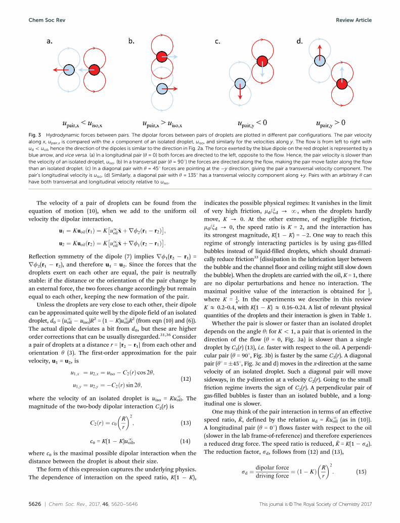
Whether the pair is slower or faster than an isolated dropletdepends on the angle y: for K o 1, a pair that is oriented in thedirection of the flow (y = 0, Fig. 3a) is slower than a singledroplet by C2(r) (13), i.e. faster with respect to the oil. A perpendi-cular pair (y = 901, Fig. 3b) is faster by the same C2(r). A diagonalpair (y1 =�451, Fig. 3c and d) moves in the x-direction at the samevelocity of an isolated droplet. Such a diagonal pair will movesideways, in the y-direction at a velocity C2(r). Going to the smallfriction regime inverts the sign of C2(r). A perpendicular pair ofgas-filled bubbles is faster than an isolated bubble, and a long-itudinal one is slower.
One may think of the pair interaction in terms of an effectivespeed ratio, K, defined by the relation ud = KuN
oil (as in (10)).A longitudinal pair (y = 01) flows faster with respect to the oil(slower in the lab frame-of-reference) and therefore experiencesa reduced drag force. The speed ratio is reduced, K = K(1 � sd).The reduction factor, sd, follows from (12) and (13),
sd ¼dipolar force
driving force¼ ð1� KÞ R
r
� �2
: (15)
Fig. 3 Hydrodynamic forces between pairs. The dipolar forces between pairs of droplets are plotted in different pair configurations. The pair velocityalong x, upair,x is compared with the x component of an isolated droplet, uiso, and similarly for the velocities along y. The flow is from left to right withud o uoil, hence the direction of the dipoles is similar to the direction in Fig. 2a. The force exerted by the blue dipole on the red droplet is represented by ablue arrow, and vice versa. (a) In a longitudinal pair (y = 0) both forces are directed to the left, opposite to the flow. Hence, the pair velocity is slower thanthe velocity of an isolated droplet, uiso. (b) In a transversal pair (y = 901) the forces are directed along the flow, making the pair move faster along the flowthan an isolated droplet. (c) In a diagonal pair with y = 451 forces are pointing at the �y direction, giving the pair a transversal velocity component. Thepair’s longitudinal velocity is uiso. (d) Similarly, a diagonal pair with y = 1351 has a transversal velocity component along +y. Pairs with an arbitrary y canhave both transversal and longitudinal velocity relative to uiso.
Chem Soc Rev Review Article
This journal is©The Royal Society of Chemistry 2017 Chem. Soc. Rev., 2017, 46, 5620--5646 | 5627
A perpendicular pair experiences an effective speed ratioincreased by the same factor. At the high friction limit,K { 1, sd is also the factor by which the effective drag coefficient,~xd, is reduced, sd E 1 � ~xd/xd E (R/r)2. The sd factor measuresthe relative strength of the dipolar interaction with respect to thedriving drag force on a single droplet. Note that sd depends onlyon the geometry, distance normalized by droplet radius, andon K. This is another demonstration that are no intrinsic scalesin this system.
The hydrodynamic dipolar forces that a pair of droplets exerton each other are equal in magnitude and direction, f12 = f21.The inter-droplet interaction violate Newton’s third law ofreciprocal actions, f12 = �f21. This is because the dipolarinteractions are effective forces that are mediated by the viscousflow, which is a non-Hamiltonian system that does not con-serve momentum and energy. One should not be confused withHamiltonian interactions, such as electrostatic dipole forces,which conserve momentum and energy and therefore obeyNewton’s third law. The electrostatic or magnetic dipole–dipoleinteraction is affected by both dipoles. In the hydrodynamicsystem, the velocity field induced by one dipole exerts a force onanother droplet.
Dipolar interactions determine the motion of dropletensembles. Ensembles of three or more droplets are no longerstable as a pair. These ensembles exhibit complicated dynamicsthat, thanks to the simplicity of the Stokes flow, can be capturedby a set of simple dynamics equations. The net hydrodynamicforce acting on a droplet is the sum of forces from all otherdroplets (Fig. 2d), a direct consequence of the linearity of Stokesflow (property (P3) in 2.2). The interaction between the i’th andthe j’th droplets (7) decays as their distance squared, 1/rij
2 withthe dipolar pattern shown in Fig. 2. From the force balance,Fdrag = �Ffric = mdud, we obtain the equation of motion of thewhole ensemble, i = 1, 2. . .N. The velocity of the i’th droplet isproportional to the oil velocity uoil(ri), which is well approxi-mated by the sum of the uniform, unperturbed flow (uN
oil) alongwith the perturbations of all other ( j a i) droplets,‡
dri
dt¼ ud rið Þ ¼ Kuoil rið Þ ¼ K u1oilxþ
Xjai
rfj ri � rj� �" #
: (16)
It is straightforward to see that the equations of motion (16),exhibit the basic properties of the Stokes flow (Section 2.2): thesolution is unique (P1), time-reversible (P2), by inverting thedriving force, and instantaneous (P4), since it depends only onthe current positions of the droplets. Moreover, it is evidentfrom the form of the equation that two solutions for the samedroplet configuration can be superimposed (P3).
By integrating the equations of motion (16), with the dipolarfields (7), one can fully determine the trajectories of the ensemble,
ri tBð Þ ¼ ri tAð Þ þÐ tBtA
dri=dtð Þdt. Numerical integration is straight-
forward and in several cases there are analytic solutions. Notethat to trace the collective motion of the ensemble there is noneed to calculate the rather intricate pattern of the streamlines.The Stokes flow enters only via the effective dipolar fields. As aresult, for most purposes, one may disregard the details of theviscous flow and treat the dynamics of driven 2D microfluidicflow by thinking of an equivalent system of particles with effectivedipolar interactions, with excluded volume interactions at shortrange. This equivalence has proved to be useful and accurate inpredicting and understanding microfluidic dynamics, as we willsee in Section 3.
2.7 The geometric origin of the inverse square law
Time does not appear explicitly in the Stokes eqn (1), whichdescribes the low-Reynolds, viscous flow. The outcome is thatthe flow velocity is determined solely by the boundary conditions.In other words, the flow is inherently geometric and lacks anatural time scale (P4). This suggests that the 1/r2 scaling of theinteraction has a geometric origin.37,38
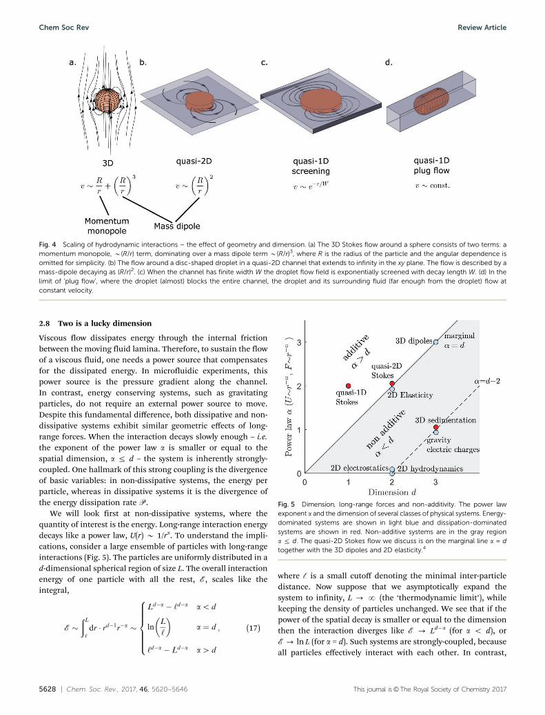
One may start the geometric consideration from the classicalexample of the viscous flow around a sphere (Fig. 4a). In 1851,George G. Stokes examined a small sphere, moving through a3D viscous fluid at constant speed.39 He found that the sphereperturbs the fluid with a velocity that decays as the inversedistance from the sphere, 1/r. In this 3D case, one can treatthe moving sphere as a point source of momentum, termed‘momentum monopole’. Since the fluid is unbounded, themomentum injected by the driven sphere is conserved. Themomentum current is rv2, and the overall flux through a shellof radius r around the sphere scales like rv2r2. By momentumconservation this flux is constant, and hence the velocity scalesas v B 1/r. Similar to the 2D droplet (Section 2.4), the spherealso induces a 3D mass-dipole that can be thought of as a pairof mass monopoles: a source and a sink. Conservation of massflux in 3D implies that the velocity induced by each massmonopole decays like 1/r2, and the 3D mass dipole flowfield scales as 1/r3, similarly to an electrostatic dipole in 3D.Therefore, the dominant perturbation of a moving sphere is the1/r momentum monopole.30,38,40
In contrast, the flow in the quasi-2D channel does notconserve the momentum, because the floor and ceilingbreak the translational symmetry along the z-axis. The lostmomentum is absorbed in the floor and ceiling boundariesvia the shear forces exerted at the edges of the Poiseuilleflow profile (Fig. 4b), owing to the velocity gradient in thez-direction.37 Unlike momentum, mass does not leak throughthe boundaries. Quite the opposite, squishing the flow to athin 2D sheet strengthens the mass dipole, since the fluidexpands only in two directions. The flow of a mass monopolein 2D is determined by the flux through a circle 2prrv = const,which implies v B 1/r. Hence, the resulting 2D dipolar fielddecays as 1/r2. Since the momentum monopole is absorbedin the floor and ceiling, the 1/r2 2D-dipole remains theleading term.31,38
‡ In principle, a full solution of the Stokes equation would require higher orderterms. The 2nd-order term accounts for perturbations of dipole strength by otherdipoles, and so on and so forth. However, the corrections scale like powers of thesmall parameter sd B (R/r)2 (15), and are therefore negligible in most cases,except for very dense droplet ensembles. Thus, (16) is an excellent approximation(see discussion in Beatus et al.,31 where exact solutions are derived).
Review Article Chem Soc Rev
5628 | Chem. Soc. Rev., 2017, 46, 5620--5646 This journal is©The Royal Society of Chemistry 2017
2.8 Two is a lucky dimension
Viscous flow dissipates energy through the internal frictionbetween the moving fluid lamina. Therefore, to sustain the flowof a viscous fluid, one needs a power source that compensatesfor the dissipated energy. In microfluidic experiments, thispower source is the pressure gradient along the channel.In contrast, energy conserving systems, such as gravitatingparticles, do not require an external power source to move.Despite this fundamental difference, both dissipative and non-dissipative systems exhibit similar geometric effects of long-range forces. When the interaction decays slowly enough – i.e.the exponent of the power law a is smaller or equal to thespatial dimension, a r d – the system is inherently strongly-coupled. One hallmark of this strong coupling is the divergenceof basic variables: in non-dissipative systems, the energy perparticle, whereas in dissipative systems it is the divergence ofthe energy dissipation rate P.
We will look first at non-dissipative systems, where thequantity of interest is the energy. Long-range interaction energydecays like a power law, U(r) B 1/ra. To understand the impli-cations, consider a large ensemble of particles with long-rangeinteractions (Fig. 5). The particles are uniformly distributed in ad-dimensional spherical region of size L. The overall interactionenergy of one particle with all the rest, E, scales like theintegral,
E �ðL‘
dr � rd�1r�a �
Ld�a � ‘d�a ao d
lnL
‘
� �a ¼ d
‘d�a � Ld�a a4 d
8>>>>><>>>>>:
; (17)
where c is a small cutoff denoting the minimal inter-particledistance. Now suppose that we asymptotically expand thesystem to infinity, L - N (the ‘thermodynamic limit’), whilekeeping the density of particles unchanged. We see that if thepower of the spatial decay is smaller or equal to the dimensionthen the interaction diverges like E - Ld�a (for a o d), orE- ln L (for a = d). Such systems are strongly-coupled, becauseall particles effectively interact with each other. In contrast,
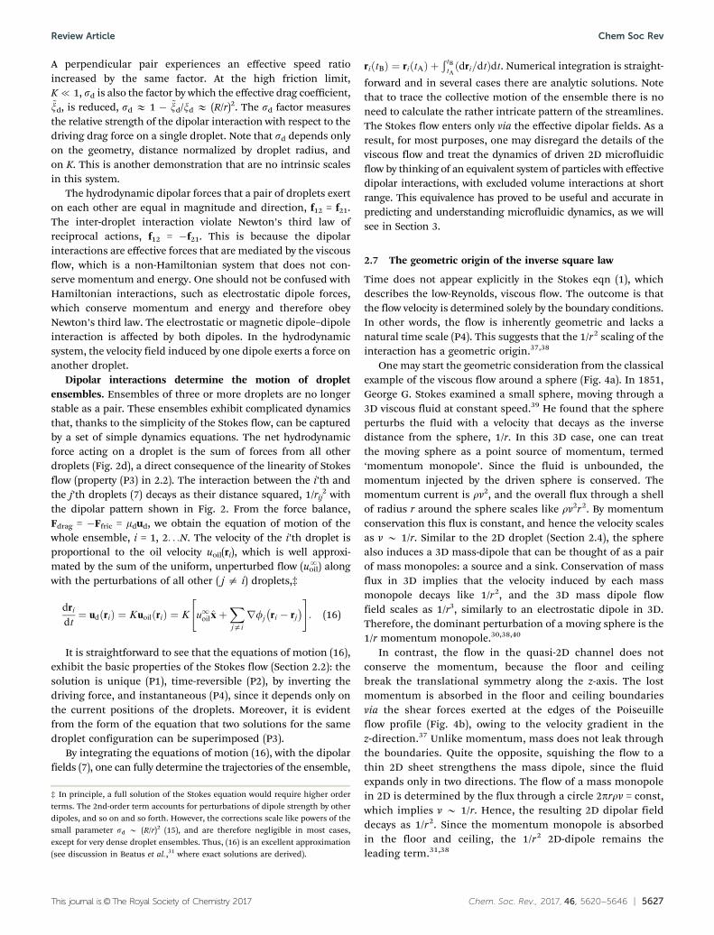
Fig. 4 Scaling of hydrodynamic interactions – the effect of geometry and dimension. (a) The 3D Stokes flow around a sphere consists of two terms: amomentum monopole, B(R/r) term, dominating over a mass dipole term B(R/r)3, where R is the radius of the particle and the angular dependence isomitted for simplicity. (b) The flow around a disc-shaped droplet in a quasi-2D channel that extends to infinity in the xy plane. The flow is described by amass-dipole decaying as (R/r)2. (c) When the channel has finite width W the droplet flow field is exponentially screened with decay length W. (d) In thelimit of ‘plug flow’, where the droplet (almost) blocks the entire channel, the droplet and its surrounding fluid (far enough from the droplet) flow atconstant velocity.
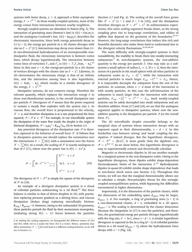
Fig. 5 Dimension, long-range forces and non-additivity. The power lawexponent a and the dimension of several classes of physical systems. Energy-dominated systems are shown in light blue and dissipation-dominatedsystems are shown in red. Non-additive systems are in the gray regiona r d. The quasi-2D Stokes flow we discuss is on the marginal line a = dtogether with the 3D dipoles and 2D elasticity.4
Chem Soc Rev Review Article
This journal is©The Royal Society of Chemistry 2017 Chem. Soc. Rev., 2017, 46, 5620--5646 | 5629
systems with faster decay, a 4 d, approach a finite asymptoticenergy, E - cd�a. In these weakly-coupled systems, most of theenergy comes from interactions between nearby neighbors.
Strongly coupled systems are abundant in Nature (Fig. 5). Theinteraction of gravitating stars (Newton’s law) is U(r) = Gm1m2/r,and the analogous Coulomb’s law, U(r) = kq1q2/r, describes theelectrostatic interaction. Since both energy potentials decay as1/r (a = 1), the energy per particle in a 3D cluster diverges withsize as EB L2 (17). Interactions may decay even slower than 1/r.In two-dimensional hydrodynamics of an incompressible non-dissipative fluid, the elementary interaction is between vortexlines, which decays logarithmically. The interaction betweenvortex lines of vorticities G1 and G2 is U(r) B G1G2 ln|r1 � r2|.41
Since in this case a = 0, the energy-per-particle in a 2D clusterof vortices diverges with the cluster size as E B L2. Likewise, in2D electrostatics the elementary charge is that of an infiniteline, and the interaction among lines is also logarithmic,U(r) B ln|r1 � r2|, which results in a similar divergence ofthe energy, E B L2.42
Dissipative systems, do not conserve energy. Therefore therelevant quantity, which replaces the interaction energy E inthese non-Hamiltonian systems, is the overall dissipation rateper particle P. Divergence of P means that the power requiredto sustain a steady flow explodes with the system size L. Inviscous flow, the overall force is proportional to the velocity,F p v, and therefore dissipation is at a rate proportional the forcesquared, P = F�v p F.2 For example, in our microfluidic systemthe dissipation of the water flow inside the droplet is the origin offrictional dissipation, P = mdud
2 = Fdrag2/md, (9) in Section 2.5.
Any potential divergence of the dissipation rate P is there-fore captured in the behavior of overall force F. It follows thatin dissipative systems one should replace the summation overthe interactions E B
PU(r), with a summation over the forces
FBP
F(r). As a result, the scaling of F is exactly analogous tothat of E (17), where now the power law is F(r) B 1/ra,§
F �ðL‘
dr � rd�1r�a ��!L!1
Ld�a ao d
lnL a ¼ d
‘d�a a4 d
8>>>>><>>>>>:
: (18)
The divergence of P BF2 is simply the square of the divergenceof F in (18).
An example of a divergent dissipative system is a cloudof colloidal particles sedimenting in a 3D fluid.43 The forcebalance is similar to that of driven droplets in 2D, with gravita-tion replacing pressure gradient as a driving force, and viscousdissipation (Stokes drag) replacing microfluidic friction:Fdrag + Fgravity = 0. However, owing to the unbounded 3D geometry,these particles perturb the fluid by their momentum monopoles,mediating strong F(r) B 1/r forces between the particles
(Section 2.7 and Fig. 4). The scaling of the overall force growslike F B L2 (a = 1 and d = 3 in (18)), and the dissipationtherefore diverges as P B F2 B L4. In sedimentation experi-ments, this naıve scaling argument breaks down, as the strongcoupling gives rise to long-range correlations, and eddies ofupflow that depend on the geometry of the boundaries.44–47
However, the long-range correlations that induce this rich andbeautiful dynamics also make them hard to understand due tothe divergent velocity fluctuations.43,44,48,49
The main difficulty with strongly-coupled systems is theirnonadditivity, the inability to break them into weakly-interactingsubsystems.4 In non-dissipative systems, the non-additivequantity is the energy per particle E. One may take as a sub-system a small sphere of radius Ls { L. If a o d, then the inter-action of a particle in the small sphere with all other particles insubsystem scales as Ein B Ld�a
s , while the interaction withexternal particles is much larger Eout BLd�a
c Ein. Hence,it is impossible decouple the subsystem from the rest of theparticles. In contrast, when a 4 d most of the interaction iswith nearby particles. In this case the self-interaction of thesubsystem is much larger than the interaction with externalparticles, Eout BLd�a
s { cd�a B Ein. Such weakly-coupledsystems can be safely decoupled into small subsystems and aretherefore additive. From (17) and (18), we see that the analogousargument applies to dissipative systems, where now the non-additive quantity is the dissipation per particle P (or the overallforce F).
The 2D microfluidic droplet ensemble belongs to themarginal class of systems whose interaction decays with anexponent equal to their dimensionality, a = d = 2. In thisborderline case between ‘strong’ and ‘weak’ coupling the dis-sipation P indeed diverges. But the logarithmic divergence,P B F2 B (ln L)2, is more gentle than the algebraic one,P B L2(d�a). As we show below, this logarithmic divergence iseasy to experimentally control and theoretically calculate.
Magnetic or electrostatic dipoles in 3D are another examplefor a marginal system in the non-dissipative realm. Owing to thelogarithmic divergence, these dipoles exhibit shape-dependentthermodynamic limits of the interaction E.50 Hydrodynamicdipoles in quasi-2D exhibit similar shape dependence that leadsto non-linear shock waves (see Section 3.5). Throughout thisreview, we will see that the marginal dimensionality allows oneto calculate a simple, first-principles theory for this strongly-coupled nonequilibrium system, while bypassing the difficultiesencountered in higher dimensions.
Importantly, d is the dimension of the particle cluster, whilethe dimension of the embedding space dspace may be larger,dspace Z d. For example, a ring of gravitating stars (a = 1) isa one-dimensional cluster, d = 1, embedded in a 3D space,dspace = 3. The scaling is determined by the cluster dimension(because the integration in (17) is over the particles), and there-fore, the gravitational energy per particle diverges logarithmicallywith the ring size, E B ln L, since a = d = 1. A similar logarithmicdivergence is expected in the in a ring (d = 1) of colloidal particlesdriven in a 3D vessel (dspace = 3), where the hydrodynamic forcedecays with a = 1 (Fig. 1d).
§ In making the scaling argument, we disregarded the different nature of U(r)and F(r): while U(r) is a scalar the force F(r) is a vector. Hence, symmetry mayaffect summation F B
PF(r) and lead to a different scaling behavior, as we will
see in Section 3.5.
Review Article Chem Soc Rev
5630 | Chem. Soc. Rev., 2017, 46, 5620--5646 This journal is©The Royal Society of Chemistry 2017
3 Emergence of collective modes
The flow of droplets in a thin channel induces long-range hydro-dynamic forces, as discussed in the previous Section 2. Theresulting dipolar interactions decay as 1/r2, which render thesystem marginal with logarithmic divergence. In the following,the reader may see several basic examples for collective modesinduced by these long-range interactions. We will start from a 1Dhydrodynamic ‘crystal’, in which phonon-like vibrations werepredicted and measured. We then look at a disordered 2D system,which exhibits sound wave and shocks that follow the Burgersequation. Finally, we look at another striking outcome of thedipolar forces, long-range orientational order which is mediatedby three-body interactions among the droplets.
3.1 Symmetry breaking makes waves in viscous media
The daily experience of viscous flow brings up the notion ofquick over-damping of any wave or oscillation by the viscous
medium.28,40,50 The persistent collective phenomena wedescribe here, phonons, waves and shock, may therefore appearcontradictory to this notion. However, as discussed below, thisapparent contradiction is because this intuition is based on ourexperience with non-driven systems that are invariant underspatial reflection. In contrast, in driven dissipative systems, likethe microfluidic droplet ensemble, the driving flow field breaksthe reflection symmetry along its direction.
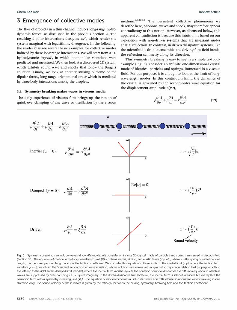
This symmetry breaking is easy to see in a simple textbookexample (Fig. 6): consider an infinite one-dimensional crystalmade of identical particles and springs, immersed in a viscousfluid. For our purpose, it is enough to look at the limit of long-wavelength modes. In this continuum limit, the dynamics ofthe crystal is governed by the second-order wave equation forthe displacement amplitude A(x,t),
r@2A
@t2þ m
@A
@t¼ k
@2A
@x2: (19)
Fig. 6 Symmetry breaking can induce waves at low-Reynolds. We consider an infinite 1D crystal made of particles and springs immersed in viscous fluid(Section 3.1). The equation of motion in the long-wavelength limit (19) contains inertial, friction, and elastic terms (top left), where k is the spring constant per unitlength, r is the mass per unit length and m is the friction coefficient. We consider this equation in three limits: in the inertial limit (top), where the friction termvanishes (m = 0), we obtain the ‘standard’ second-order wave equation, whose solutions are waves with a symmetric dispersion relation that propagate both tothe left and to the right. In the damped limit (middle), where the inertial term vanishes (r = 0) the equation of motion becomes the diffusion equation, in which allwaves are suppressed by over-damping, i.e. o is pure imaginary. In the driven-dissipative limit (bottom), the inertial term is still not included, but we replace theharmonic term with a symmetry-breaking field xqxA. The equation of motion becomes a first-order wave eqn (20), whose solutions are waves traveling in onedirection only. The sound velocity of these waves is given by the ratio x/m between the driving, symmetry-breaking field and the friction coefficient.
Chem Soc Rev Review Article
This journal is©The Royal Society of Chemistry 2017 Chem. Soc. Rev., 2017, 46, 5620--5646 | 5631
The first term is the inertia with the mass per length r,the second term is the friction force with the friction coeffi-cient m, and the third term is the elastic force with the springconstant k. Eqn (19) is symmetric with respect to a x - �xreflection.
In the inertial, frictionless regime, eqn (19) becomes thestandard wave equation, r(q2A/qt2) = k(q2A/qx2). Because of thex-reflection symmetry (or the time-reversal symmetry, t - �t),there are both leftward and rightward propagating waves,
A(x,t) B f (x � Cst), with a sound velocity Cs ¼ffiffiffiffiffiffiffiffik=r
p. Reflection
symmetry also implies that the spectrum of the harmonicwaves, A(x,t) B exp[i(kx � ot)], is symmetric around k = 0,o(k) = Cs|k|. At the other extreme, when dissipation dominatesinertia, eqn (19) becomes the diffusion equation, m(qA/qt) =k(q2A/qx2). This is the Stokes regime, Re { 1, where all waves aresuppressed by over-damping, o(k) = i(k/m)k2. Such over-dampeddynamics was measured in systems of colloidal particles.51
Nevertheless, waves can still be excited in the viscous regimeby introducing a symmetry-breaking field to the equationof motion. For example, we may replace the harmonic springforce k(q2A/qx2) by a driving force, x(qA/qx). This linear term isasymmetric with respect to x-reflection. In the dissipation-dominated limit, the equation of motion (19) becomes a first-order wave equation,
x@A
@x¼ m
@A
@t: (20)
This is the simplest possible wave equation, and one may askhow come it is much less familiar than the second-order equationusually called the ‘‘wave equation’’. The answer is that it requiresan additional symmetry-breaking force, which renders the systemnon-Hamiltonian.52,53
Because of its broken symmetry, the first-order wave equa-tion exhibits unidirectional traveling waves solutions, A(x,t) Bf (x � Cst), with the sound speed Cs = x/m. These solutions aremarkedly different than waves in common elastic materials,where a local perturbation will send waves in all directions. In acrystal described by (20), waves propagate only in a directiondetermined by the symmetry-breaking force. The plane wavespectrum is antisymmetric in k, o(k) = Csk (Fig. 6). In an elasticcrystal, the forces exerted by the downstream and upstreamneighbors are opposite in sign, which leads to the second orderinteraction, k(q2A/qx2). In contrast, the forces in the microflui-dic crystal all point in the same direction, which is the origin ofthe linear force, x(qA/qx). Moreover, we will see in the following(Section 3.3) that the long wavelength limit of the hydrodynamiccrystal obeys the same 1st-order wave equation. In summary,waves can still persist in the viscous regime, provided that thereis symmetry-breaking driving force.
3.2 Moving microfluidic crystals: the peloton effect
The simplest droplet ensemble is an infinite one-dimensionalarray along the flow direction, with uniform spacing a betweenadjacent droplets (Fig. 1a). Interestingly, all array parameters(a, R, ud, uoil) are imposed by the droplet formation process andnot determined by any equilibration process. Such an array is
termed ‘microfluidic crystal’ because, as we show below, similarlyto a solid-state crystal, it exhibits phonon-like collective vibra-tional modes due to the interactions between the droplets.However, the modes of the microfluidic crystal are markedlydifferent than those of its solid-state counterpart.
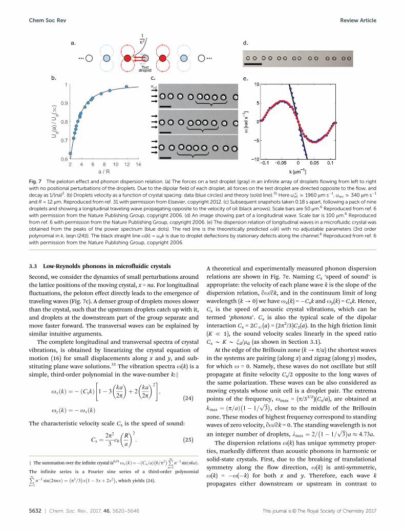
First, we consider a crystal moving steadily in the directionof the flow without any deviations of the droplets with respect totheir crystal positions (Fig. 7a and b). We have seen in Section 2.6that a pair of droplets oriented parallel to the flow is slower thanan isolated droplet by C2(r) (13), due to dipolar interaction. In thecrystal, there are similar interactions between all pairs of dro-plets, since every droplet is subject to the hydrodynamic forcesof all other droplets. The symmetry of the dipolar force fieldimplies that all forces on a test droplet are directed in the samedirection, opposite to the flow. Namely, a droplet located ncrystal spacings downstream of the test droplet exerts the sameforce, in both magnitude and direction, as a droplet located naupstream. Consequently, all droplets experience a force oppositeto the flow and the entire crystal moves slower than an isolateddroplet. Since the dipolar force decays as r�2, a dense crystalexhibits stronger inter-droplet forces and moves slower than asparse crystal. The crystal velocity as a function of its spacing isobtained from (16) with rn = nax:
udðaÞ ¼Ku1oil
1þ p2
3ð1� KÞ R
a
� �2 uiso � C1ðaÞ; (21)
where the slowdown in (21) with respect to the isolated dropletvelocity uiso = KuN
oil is
C1ðaÞ ¼p2
3c0
R
a
� �2
; (22)
where c0 � K(1 � K)uN
oil as in (14). Although all inter-dropletforces are directed upstream, the crystal still flows downstreamdue to the drag force exerted on each droplet by the carrierfluid, which is stronger than the sum of all inter-droplet forces.In the frame-of-reference of the carrier fluid, as a decreases thecrystal moves faster, a phenomenon known as collective dragreduction. By analogy to cyclists riding faster as a pack at a highReynolds number regime, we term this low-Re drag reductionphenomenon the ‘peloton’ effect.
The peloton effect (22) scales like the pair slowdown (13),CN(a) = (p2/3)�C2(a). The factor p2/3, reflects the summationover the 1/r2 contributions of the infinite crystal.¶ In themoving crystal, the speed ratio K is reduced to an effectivevalue, K, by a factor
K � ~K
K p2
3ð1� KÞ R
a
� �2
: (23)
At the high friction limit, K { 1, this is also the reduction of theeffective drag coefficient, ~xd, by a factor (xd� ~xd)/xd E (p2/3)(R/a)2.
¶ The sum over the crystal is p2=3 ¼P11
n�2 þP�1�1
n�2. Most of the interaction is
with the two nearest neighbors. The rest of the crystal contributes B40%. Thisimplies that the interaction within the 1D structure are effectively short-ranged.
Review Article Chem Soc Rev
5632 | Chem. Soc. Rev., 2017, 46, 5620--5646 This journal is©The Royal Society of Chemistry 2017
3.3 Low-Reynolds phonons in microfluidic crystals
Second, we consider the dynamics of small perturbations aroundthe lattice positions of the moving crystal, x = na. For longitudinalfluctuations, the peloton effect directly leads to the emergence oftraveling waves (Fig. 7c). A denser group of droplets moves slowerthan the crystal, such that the upstream droplets catch up with it,and droplets at the downstream part of the group separate andmove faster forward. The transversal waves can be explained bysimilar intuitive arguments.
The complete longitudinal and transversal spectra of crystalvibrations, is obtained by linearizing the crystal equation ofmotion (16) for small displacements along x and y, and sub-stituting plane wave solutions.31 The vibration spectra o(k) is asimple, third-order polynomial in the wave-number k:8
oxðkÞ ¼ � Cskð Þ 1� 3ka
2p
� �þ 2
ka
2p
� �2" #
;
oyðkÞ ¼ � oxðkÞ
(24)
The characteristic velocity scale Cs is the speed of sound:
Cs ¼2p2
3c0
R
a
� �2
: (25)
A theoretical and experimentally measured phonon dispersionrelations are shown in Fig. 7e. Naming Cs ‘speed of sound’ isappropriate: the velocity of each plane wave k is the slope of thedispersion relation, qo/qk, and in the continuum limit of longwavelength (k - 0) we have ox(k) =�Csk and oy(k) = Csk. Hence,Cs is the speed of acoustic crystal vibrations, which can betermed ‘phonons’. Cs is also the typical scale of the dipolarinteraction Cs = 2CN(a) = (2p2/3)C2(a). In the high friction limit(K { 1), the sound velocity scales linearly in the speed ratioCs B K B xd/md (as shown in Section 3.1).
At the edge of the Brillouin zone (k - p/a) the shortest wavesin the systems are pairing (along x) and zigzag (along y) modes,for which o = 0. Namely, these waves do not oscillate but stillpropagate at finite velocity Cs/2 opposite to the long waves ofthe same polarization. These waves can be also considered asmoving crystals whose unit cell is a droplet pair. The extremapoints of the frequency, omax = (p/33/2)(Cs/a), are obtained at
kmax ¼ ðp=aÞ 1� 1=ffiffiffi3p� �
, close to the middle of the Brillouinzone. These modes of highest frequency correspond to standingwaves of zero velocity, qo/qk = 0. The standing wavelength is not
an integer number of droplets, lmax ¼ 2= 1� 1=ffiffiffi3p� �
a 4:73a.The dispersion relations o(k) has unique symmetry proper-
ties, markedly different than acoustic phonons in harmonic orsolid-state crystals. First, due to the breaking of translationalsymmetry along the flow direction, o(k) is anti-symmetric,o(k) = �o(�k) for both x and y. Therefore, each wave kpropagates either downstream or upstream in contrast to
Fig. 7 The peloton effect and phonon dispersion relation. (a) The forces on a test droplet (gray) in an infinite array of droplets flowing from left to rightwith no positional perturbations of the droplets. Due to the dipolar field of each droplet, all forces on the test droplet are directed opposite to the flow, anddecay as 1/(na)2. (b) Droplets velocity as a function of crystal spacing: data (blue circles) and theory (solid line).31 Here uN
oil C 1960 mm s�1, uiso C 340 mm s�1
and R = 12 mm. Reproduced from ref. 31 with permission from Elsevier, copyright 2012. (c) Subsequent snapshots taken 0.18 s apart, following a pack of ninedroplets and showing a longitudinal traveling wave propagating opposite to the velocity of oil (black arrows). Scale bars are 50 mm.6 Reproduced from ref. 6with permission from the Nature Publishing Group, copyright 2006. (d) An image showing part of a longitudinal wave. Scale bar is 100 mm.6 Reproducedfrom ref. 6 with permission from the Nature Publishing Group, copyright 2006. (e) The dispersion relation of longitudinal waves in a microfluidic crystal wasobtained from the peaks of the power spectrum (blue dots). The red line is the theoretically predicted o(k) with no adjustable parameters (3rd orderpolynomial in k, (eqn (24))). The black straight line o(k) = udk is due to droplet deflections by stationary defects along the channel.6 Reproduced from ref. 6with permission from the Nature Publishing Group, copyright 2006.
8 The summation over the infinite crystal is6,31 oxðkÞ¼� Cs=að Þ 6=p2� �P1
n¼1n�3 sinðnkaÞ.
The infinite series is a Fourier sine series of a third-order polynomialP1n¼1
n�3 sinð2pnxÞ ¼ p3=3� �
x 1� 3xþ 2x2� �
, which yields (24).
Chem Soc Rev Review Article
This journal is©The Royal Society of Chemistry 2017 Chem. Soc. Rev., 2017, 46, 5620--5646 | 5633
harmonic crystals, in which o(k) = o(�k) and each wave kpropagates in both directions. This is exactly the antisymmetrypredicted in Section 3.1 on the basis of simple symmetryarguments. Second, the dispersion is also anti-symmetric withrespect to polarization, oy(k) =�ox(k). This property stems fromthe fact that the equations of motion for x and y are identicalup to a sign, which is a hallmark of potential equations suchas eqn (4).
The spectra was measured by tracking the positions of thedroplets in a frame of reference moving with the crystal.6 Thepower-spectra (Fig. 7e) were obtained by calculating the spatialand temporal Fourier transforms of the droplets x and y positions.The power spectra show the amplitude of each plane wave,as described by its temporal frequency o and spatial wave-number k. The peaks of the power spectra represent the normalmodes of the crystal, which are the dispersion relations ox(k)and oy(k). Remarkably, the measured o(k) is in perfect agree-ment with the theoretical prediction without any fit parameters.In such experiments the characteristic phonon frequency isabout 1 Hz and sound velocity is Cs E 250 mm s�1, which isabout 6 orders of magnitude slower than sound speed in thefluid. Similar phonon spectra have later been observed in othersystems (Fig. 8).
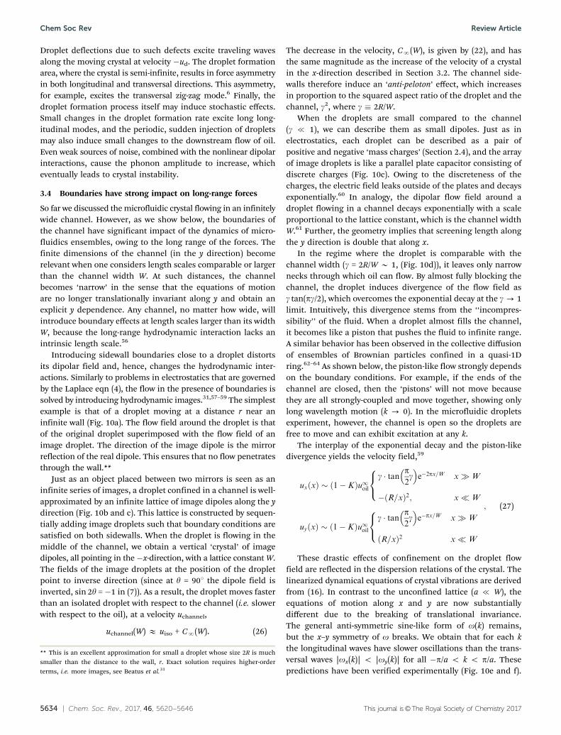
Unstable crystals. Beyond the small amplitude approxi-mation in an infinite crystal, the system exhibits several modesof instability. The force asymmetry near the droplet formationedge leads to crystal instability in which the zigzag mode grows,splitting the crystal into two interlacing crystals (Fig. 9a). A secondmode of instability stems from the nonlinear coupling betweenlongitudinal and transversal waves. This coupling leads to crystalbreakup by the rapid growth of a distinct configuration ofB4 droplets (Fig. 9b), in the vicinity of the highest frequencystanding waves (lmax = E4.73a). These modes of instability arereproduced by numerical solution of the nonlinear equations ofmotion (16). Similar unstable modes have been predicted in a
lattice of drifting vortices in type-II superconductor,53 and werepreviously shown in sedimenting particles.52
Sources of noise. While phonons are excited at all wave-lengths, the source for these excitations is not be thermal, sincethe droplets are too large and over-damped such that thermalfluctuations are negligible (Section 2.5). Noise in this systemstems from several sources. Defects along the channel locallychange the flow of oil, thus modify the hydrodynamic dipoles.
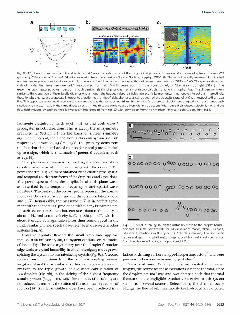
Fig. 8 1D phonon spectra in additional systems. (a) Numerical calculation of the longitudinal phonon dispersion of an array of spheres in quasi-2Dgeometry.54 Reproduced from ref. 54 with permission from the American Physical Society, copyright 2008. (b) The experimentally measured longitudinaland transversal power spectra of a microfluidic crystal confined in a narrow channel, with confinement parameter g = 2R/W = 0.66. The spectra show twodistinct modes that have been excited.55 Reproduced from ref. 55 with permission from the Royal Society of Chemistry, copyright 2015. (c) Theexperimentally measured power spectrum and dispersion relation of phonons in a ring of micro-particles rotating in an optical trap. The dispersion is verysimilar to the dispersion of the microfluidic phonons, although the trapped micro-particles interact via 1/r momentum monopole interactions. Interestingly,these longitudinal waves propagate in opposite direction to the microfluidic phonons, as can be seen by the opposite slope of o(k) with respect to the�ud�kline. The opposite sign of the dispersion stems from the way the particles are driven. In the microfluidic crystal droplets are dragged by the oil, hence theirrelative velocity uoil� ud is in the same direction as ud. In the ring, the particles are driven within a quiescent fluid, hence their relative velocity is�ud and theflow field induced by each particle is inversed.10 Reproduced from ref. 10 with permission from the American Physical Society, copyright 2014.
Fig. 9 Crystal instability. (a) Zigzag instability close to the droplet forma-tion area. All scale-bars are 100 mm. (b) Subsequent images, taken 0.3 s apart,of a local fluctuation in a 1D crystal (1 + 3 droplets, marked). The fluctuationgrows and leads to crystal breakup. Reproduced from ref. 6 with permissionfrom the Nature Publishing Group, copyright 2006.
Review Article Chem Soc Rev
5634 | Chem. Soc. Rev., 2017, 46, 5620--5646 This journal is©The Royal Society of Chemistry 2017
Droplet deflections due to such defects excite traveling wavesalong the moving crystal at velocity �ud. The droplet formationarea, where the crystal is semi-infinite, results in force asymmetryin both longitudinal and transversal directions. This asymmetry,for example, excites the transversal zig-zag mode.6 Finally, thedroplet formation process itself may induce stochastic effects.Small changes in the droplet formation rate excite long long-itudinal modes, and the periodic, sudden injection of dropletsmay also induce small changes to the downstream flow of oil.Even weak sources of noise, combined with the nonlinear dipolarinteractions, cause the phonon amplitude to increase, whicheventually leads to crystal instability.
3.4 Boundaries have strong impact on long-range forces
So far we discussed the microfluidic crystal flowing in an infinitelywide channel. However, as we show below, the boundaries ofthe channel have significant impact of the dynamics of micro-fluidics ensembles, owing to the long range of the forces. Thefinite dimensions of the channel (in the y direction) becomerelevant when one considers length scales comparable or largerthan the channel width W. At such distances, the channelbecomes ‘narrow’ in the sense that the equations of motionare no longer translationally invariant along y and obtain anexplicit y dependence. Any channel, no matter how wide, willintroduce boundary effects at length scales larger than its widthW, because the long-range hydrodynamic interaction lacks anintrinsic length scale.56
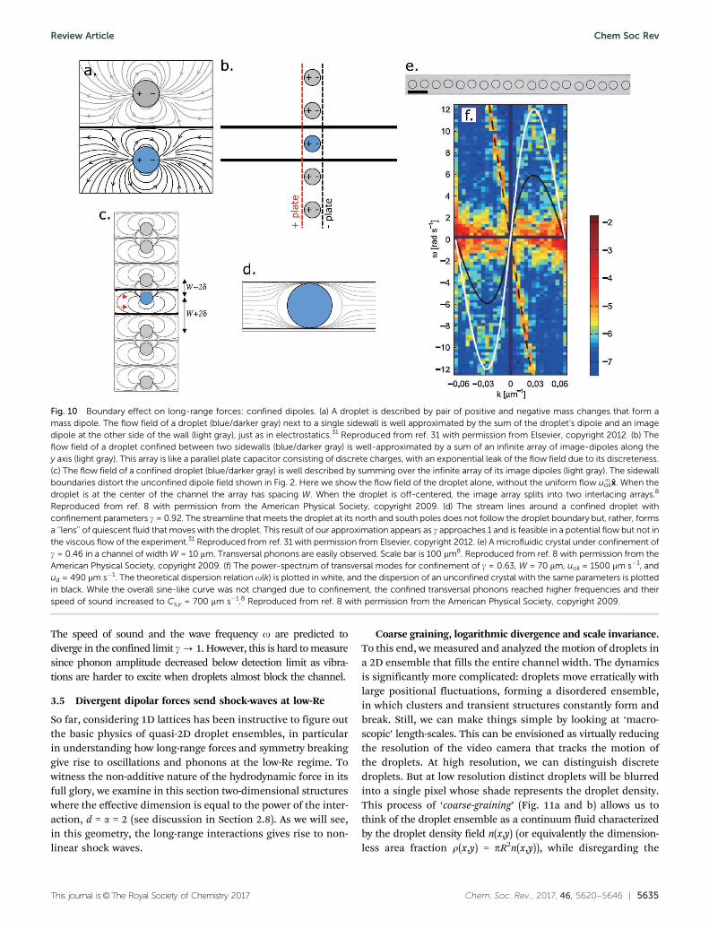
Introducing sidewall boundaries close to a droplet distortsits dipolar field and, hence, changes the hydrodynamic inter-actions. Similarly to problems in electrostatics that are governedby the Laplace eqn (4), the flow in the presence of boundaries issolved by introducing hydrodynamic images.31,57–59 The simplestexample is that of a droplet moving at a distance r near aninfinite wall (Fig. 10a). The flow field around the droplet is thatof the original droplet superimposed with the flow field of animage droplet. The direction of the image dipole is the mirrorreflection of the real dipole. This ensures that no flow penetratesthrough the wall.**
Just as an object placed between two mirrors is seen as aninfinite series of images, a droplet confined in a channel is well-approximated by an infinite lattice of image dipoles along the ydirection (Fig. 10b and c). This lattice is constructed by sequen-tially adding image droplets such that boundary conditions aresatisfied on both sidewalls. When the droplet is flowing in themiddle of the channel, we obtain a vertical ‘crystal’ of imagedipoles, all pointing in the�x-direction, with a lattice constant W.The fields of the image droplets at the position of the dropletpoint to inverse direction (since at y = 901 the dipole field isinverted, sin 2y = �1 in (7)). As a result, the droplet moves fasterthan an isolated droplet with respect to the channel (i.e. slowerwith respect to the oil), at a velocity uchannel,
uchannel(W) E uiso + CN(W). (26)
The decrease in the velocity, CN(W), is given by (22), and hasthe same magnitude as the increase of the velocity of a crystalin the x-direction described in Section 3.2. The channel side-walls therefore induce an ‘anti-peloton’ effect, which increasesin proportion to the squared aspect ratio of the droplet and thechannel, g2, where g � 2R/W.
When the droplets are small compared to the channel(g { 1), we can describe them as small dipoles. Just as inelectrostatics, each droplet can be described as a pair ofpositive and negative ‘mass charges’ (Section 2.4), and the arrayof image droplets is like a parallel plate capacitor consisting ofdiscrete charges (Fig. 10c). Owing to the discreteness of thecharges, the electric field leaks outside of the plates and decaysexponentially.60 In analogy, the dipolar flow field around adroplet flowing in a channel decays exponentially with a scaleproportional to the lattice constant, which is the channel widthW.61 Further, the geometry implies that screening length alongthe y direction is double that along x.
In the regime where the droplet is comparable with thechannel width (g = 2R/W B 1, (Fig. 10d)), it leaves only narrownecks through which oil can flow. By almost fully blocking thechannel, the droplet induces divergence of the flow field asg tan(pg/2), which overcomes the exponential decay at the g- 1limit. Intuitively, this divergence stems from the ‘‘incompres-sibility’’ of the fluid. When a droplet almost fills the channel,it becomes like a piston that pushes the fluid to infinite range.A similar behavior has been observed in the collective diffusionof ensembles of Brownian particles confined in a quasi-1Dring.62–64 As shown below, the piston-like flow strongly dependson the boundary conditions. For example, if the ends of thechannel are closed, then the ‘pistons’ will not move becausethey are all strongly-coupled and move together, showing onlylong wavelength motion (k - 0). In the microfluidic dropletsexperiment, however, the channel is open so the droplets arefree to move and can exhibit excitation at any k.
The interplay of the exponential decay and the piston-likedivergence yields the velocity field,59
uxðxÞ � ð1� KÞu1oilg � tan p
2g
�e�2px=W xW
�ðR=xÞ2; x�W
8<:
uyðxÞ � ð1� KÞu1oilg � tan p
2g
�e�px=W xW
ðR=xÞ2 x�W
8<:
; (27)
These drastic effects of confinement on the droplet flowfield are reflected in the dispersion relations of the crystal. Thelinearized dynamical equations of crystal vibrations are derivedfrom (16). In contrast to the unconfined lattice (a { W), theequations of motion along x and y are now substantiallydifferent due to the breaking of translational invariance.The general anti-symmetric sine-like form of o(k) remains,but the x–y symmetry of o breaks. We obtain that for each kthe longitudinal waves have slower oscillations than the trans-versal waves |ox(k)| o |oy(k)| for all �p/a o k o p/a. Thesepredictions have been verified experimentally (Fig. 10e and f).
** This is an excellent approximation for small a droplet whose size 2R is muchsmaller than the distance to the wall, r. Exact solution requires higher-orderterms, i.e. more images, see Beatus et al.31
Chem Soc Rev Review Article
This journal is©The Royal Society of Chemistry 2017 Chem. Soc. Rev., 2017, 46, 5620--5646 | 5635
The speed of sound and the wave frequency o are predicted todiverge in the confined limit g- 1. However, this is hard to measuresince phonon amplitude decreased below detection limit as vibra-tions are harder to excite when droplets almost block the channel.
3.5 Divergent dipolar forces send shock-waves at low-Re
So far, considering 1D lattices has been instructive to figure outthe basic physics of quasi-2D droplet ensembles, in particularin understanding how long-range forces and symmetry breakinggive rise to oscillations and phonons at the low-Re regime. Towitness the non-additive nature of the hydrodynamic force in itsfull glory, we examine in this section two-dimensional structureswhere the effective dimension is equal to the power of the inter-action, d = a = 2 (see discussion in Section 2.8). As we will see,in this geometry, the long-range interactions gives rise to non-linear shock waves.
Coarse graining, logarithmic divergence and scale invariance.To this end, we measured and analyzed the motion of droplets ina 2D ensemble that fills the entire channel width. The dynamicsis significantly more complicated: droplets move erratically withlarge positional fluctuations, forming a disordered ensemble,in which clusters and transient structures constantly form andbreak. Still, we can make things simple by looking at ‘macro-scopic’ length-scales. This can be envisioned as virtually reducingthe resolution of the video camera that tracks the motion ofthe droplets. At high resolution, we can distinguish discretedroplets. But at low resolution distinct droplets will be blurredinto a single pixel whose shade represents the droplet density.This process of ‘coarse-graining’ (Fig. 11a and b) allows us tothink of the droplet ensemble as a continuum fluid characterizedby the droplet density field n(x,y) (or equivalently the dimension-less area fraction r(x,y) = pR2n(x,y)), while disregarding the
Fig. 10 Boundary effect on long-range forces: confined dipoles. (a) A droplet is described by pair of positive and negative mass changes that form amass dipole. The flow field of a droplet (blue/darker gray) next to a single sidewall is well approximated by the sum of the droplet’s dipole and an imagedipole at the other side of the wall (light gray), just as in electrostatics.31 Reproduced from ref. 31 with permission from Elsevier, copyright 2012. (b) Theflow field of a droplet confined between two sidewalls (blue/darker gray) is well-approximated by a sum of an infinite array of image-dipoles along they axis (light gray). This array is like a parallel plate capacitor consisting of discrete charges, with an exponential leak of the flow field due to its discreteness.(c) The flow field of a confined droplet (blue/darker gray) is well described by summing over the infinite array of its image dipoles (light gray). The sidewallboundaries distort the unconfined dipole field shown in Fig. 2. Here we show the flow field of the droplet alone, without the uniform flow uN
oilx. When thedroplet is at the center of the channel the array has spacing W. When the droplet is off-centered, the image array splits into two interlacing arrays.8
Reproduced from ref. 8 with permission from the American Physical Society, copyright 2009. (d) The stream lines around a confined droplet withconfinement parameters g = 0.92. The streamline that meets the droplet at its north and south poles does not follow the droplet boundary but, rather, formsa ‘‘lens’’ of quiescent fluid that moves with the droplet. This result of our approximation appears as g approaches 1 and is feasible in a potential flow but not inthe viscous flow of the experiment.31 Reproduced from ref. 31 with permission from Elsevier, copyright 2012. (e) A microfluidic crystal under confinement ofg = 0.46 in a channel of width W = 10 mm. Transversal phonons are easily observed. Scale bar is 100 mm8. Reproduced from ref. 8 with permission from theAmerican Physical Society, copyright 2009. (f) The power-spectrum of transversal modes for confinement of g = 0.63, W = 70 mm, uoil = 1500 mm s�1, andud = 490 mm s�1. The theoretical dispersion relation o(k) is plotted in white, and the dispersion of an unconfined crystal with the same parameters is plottedin black. While the overall sine-like curve was not changed due to confinement, the confined transversal phonons reached higher frequencies and theirspeed of sound increased to Cs,y = 700 mm s�1.8 Reproduced from ref. 8 with permission from the American Physical Society, copyright 2009.
Review Article Chem Soc Rev
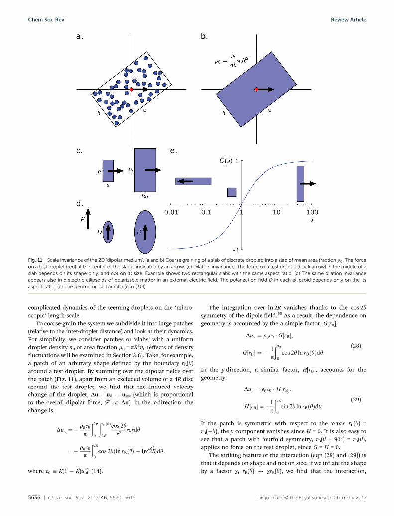
5636 | Chem. Soc. Rev., 2017, 46, 5620--5646 This journal is©The Royal Society of Chemistry 2017
complicated dynamics of the teeming droplets on the ‘micro-scopic’ length-scale.
To coarse-grain the system we subdivide it into large patches(relative to the inter-droplet distance) and look at their dynamics.For simplicity, we consider patches or ‘slabs’ with a uniformdroplet density n0 or area fraction r0 = pR2n0 (effects of densityfluctuations will be examined in Section 3.6). Take, for example,a patch of an arbitrary shape defined by the boundary rB(y)around a test droplet. By summing over the dipolar fields overthe patch (Fig. 11), apart from an excluded volume of a 4R discaround the test droplet, we find that the induced velocitychange of the droplet, Du = ud � uiso (which is proportionalto the overall dipolar force, F p Du). In the x-direction, thechange is
Dux ¼�r0c0p
ð2p0
ðrBðyÞ2R
cos 2yr2
rdrdy
¼� r0c0p
ð2p0
cos 2yðln rBðyÞ � In 2R
/
Þdy;
where c0 � K(1 � K)uN
oil (14).
The integration over ln 2R vanishes thanks to the cos 2ysymmetry of the dipole field.65 As a result, the dependence ongeometry is accounted by the a simple factor, G[rB],
Dux ¼ r0c0 � G rB½ �;
G rB½ � ¼ �1
p
ð2p0
cos 2y ln rBðyÞdy:(28)
In the y-direction, a similar factor, H[rB], accounts for thegeometry,
Duy ¼ r0c0 �H rB½ �;
H½rB� ¼ �1
p
ð2p0
sin 2y ln rBðyÞdy:(29)
If the patch is symmetric with respect to the x-axis rB(y) =rB(�y), the y component vanishes since H = 0. It is also easy tosee that a patch with fourfold symmetry, rB(y + 901) = rB(y),applies no force on the test droplet, since G = H = 0.
The striking feature of the interaction (eqn (28) and (29)) isthat it depends on shape and not on size: if we inflate the shapeby a factor w, rB(y) - wrB(y), we find that the interaction,
Fig. 11 Scale invariance of the 2D ‘dipolar medium’. (a and b) Coarse graining of a slab of discrete droplets into a slab of mean area fraction r0. The forceon a test droplet (red) at the center of the slab is indicated by an arrow. (c) Dilation invariance. The force on a test droplet (black arrow) in the middle of aslab depends on its shape only, and not on its size. Example shows two rectangular slabs with the same aspect ratio. (d) The same dilation invarianceappears also in dielectric ellipsoids of polarizable matter in an external electric field. The polarization field D in each ellipsoid depends only on the itsaspect ratio. (e) The geometric factor G(s) (eqn (30)).
Chem Soc Rev Review Article
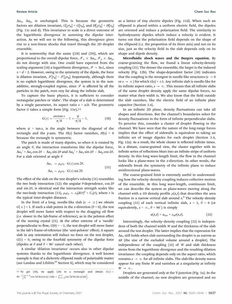
This journal is©The Royal Society of Chemistry 2017 Chem. Soc. Rev., 2017, 46, 5620--5646 | 5637
Dux, Duy, is unchanged. This is because the geometricfactors are dilation invariant, G[wrB] = G[rB], and H[wrB] = H[rB](Fig. 11c and d). This invariance to scale is a direct outcome ofthe logarithmic divergence in summing the dipolar inter-action. As we will see in the following, this divergence givesrise to a non-linear shocks that travel through the 2D dropletensemble.
It is noteworthy that the sums ((28) and (29)), which areproportional to the overall dipolar force, Fx p Dux, Fy p Duy,do not diverge with size. One could have expected from thescaling argument (18) a logarithmic divergence, FB ln L, sincea = d = 2. However, owing to the symmetry of the dipole, the forceis dilation invariant, F[rB] = F[wrB]. Importantly, although thereis no explicit logarithmic divergence, the system is in the non-additive, strongly-coupled regime, since F is affected by all theparticles in the patch, even very far along the infinite slab.
To capture the basic physics, it is sufficient to considerrectangular patches or ‘slabs’. The shape of a slab is determinedby a single parameter, its aspect ratio s = a/b. The geometricfactor G takes a simple form (Fig. 11e),††
GðsÞ ¼ arctan s
p=4� 1 ¼ c
p=4� 1; (30)
where c = tan s, is the angle between the diagonal of therectangle and the y-axis. The H(s) factor vanishes, H(s) = 0because the rectangle is symmetric.
The patch is made of many dipoles, so when it is rotated byan angle y, the interaction transforms like the dipolar force,Dux
0 = Dux cos 2y � Duy sin 2y and Duy0 = Dux sin 2y � Duy cos 2y.
For a slab oriented at angle y
Dux ¼ r0c0 � GðsÞ cos 2y;
Duy ¼ r0c0 � GðsÞ sin 2y:(31)
The effect of the slab on the test droplet’s velocity (31) resemblesthe two body interaction (12): the angular y-dependence, cos 2yand sin 2y, is identical and the interaction strength scales likethe two-body interaction (13), r0c0 B c0(R/r)2 = C2(r), where r isthe typical inter-droplet distance.
In the limit of a long, needle-like slab (s - N) we obtainG(N) = 1. If such a slab points in the x-direction (y = 0), the testdroplet will move faster with respect to the dragging oil flow(i.e. slower in the lab-frame of reference), as in the peloton effectof the moving crystal (21). At the other extreme of a ‘needle’perpendicular to flow, G(0) = �1, the test droplet will move fasterin the lab’s frame-of-reference (the ‘anti-peloton’ effect). A squareslab in any orientation will induce no force on the test droplet,G(1) = 0, owing to the fourfold symmetry of the dipolar force(dipoles at y and y + 901 cancel each other).
A similar ‘dilation invariance’ occurs also in other dipolarsystems thanks to the logarithmic divergence. A well knownexample is that of a dielectric ellipsoid made of polarizable matter(see Landau and Lifshitz50 Section 8), which may be considered
as a lattice of tiny electric dipoles (Fig. 11d). When such anellipsoid is placed within a uniform electric field, the dipolesare oriented and induce a polarization field. The similarity tohydrodynamic dipoles which induce a velocity is evident. Itturns out that the polarization field depends on the shape ofthe ellipsoid (i.e. the proportion of its three axis) and not on itssize, just as the velocity field in the slab depends only on itsshape and dipole density.
Microfluidic shock waves and the Burgers equation. Bycoarse-graining the flow, we found a linear velocity-densitycoupling (31). The denser the ensemble, the larger is the inducedvelocity (Fig. 12b). The shape-dependent factor (30) indicatesthat the coupling is the strongest in needle-like structures (s - 0or s -N) for which G(s) =�1. Any infinite slab is needle-like forits infinite aspect ratio, s -N. This means that all infinite slabsof the same droplet density apply the same dipolar forces, nomatter what their width is. We also know that the field outsidethe slab vanishes, like the electric field of an infinite platecapacitor (Section 3.4).
In an infinite 2D plane, density fluctuations can take allshapes and directions. But the channel’s boundaries select fordensity fluctuations in the form of infinite perpendicular slabs.To perceive this, consider a cluster of droplet flowing in thechannel. We have seen that the nature of the long-range forcesimplies that the effect of sidewalls is equivalent to taking aninfinite set of image dipoles for each droplet (Section 3.4,Fig. 12a). As a result, the whole cluster is reflected infinite times.In a distant, coarse-grained view, the cluster together with itsinfinite series of reflections blurs into an infinite stripe of uniformdensity. In this long wave-length limit, the flow in the channellooks like a plane-wave in the x-direction. In other words, thesidewalls break the symmetry of the infinite plane to induceunidirectional plane-waves.
The coarse-grained limit is extremely useful in understand-ing how the velocity–density coupling induces collective motionof the ensemble. At this long wave-length, continuum limit,we can describe the system as plane-waves moving along thechannel with a 1D density profile r(x,t) that describes the areafraction in a narrow vertical slab around x.8 The velocity–densitycoupling (31) of each vertical infinite slab, s = 1, y = 0 (orequivalently, s = N, y = 901) is simply
u(x,t) = uiso + c0r(x,t). (32)
Interestingly, the velocity–density coupling (32) is indepen-dent of both the channel width W and the thickness of the slabaround the test droplet. The latter implies that the expression forDux still holds when slab surrounding the droplet is as narrow as4R (the size of the excluded volume around a droplet). Theindependence of the coupling (32) of W and slab thicknessstems from the logarithmic divergence and the resulting dilationinvariance: the coupling depends only on the aspect ratio, whichremains s -N for all infinite slabs. The slab-like density wavesappear for any finite W and vanishes at a singularity at infinityW - N.
Droplets are generated only at the T-junction (Fig. 1a). In themiddle of the channel, no new droplets are generated and no
†† To get (30), we apply (28) to a rectangle and obtain GðsÞ ¼
4p�1Ð p=2�c0 cos 2f lnðcosf=sÞdfþ
Ð p=2p=2�ccos 2f lnðsinfÞdf
h i.
Review Article Chem Soc Rev
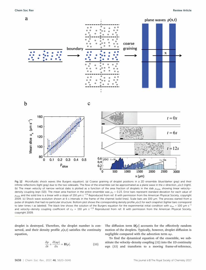
5638 | Chem. Soc. Rev., 2017, 46, 5620--5646 This journal is©The Royal Society of Chemistry 2017
droplet is destroyed. Therefore, the droplet number is con-served, and their density profile r(x,t) satisfies the continuityequation,
@r@tþ @ðurÞ
@x¼ D½r�: (33)
The diffusion term D[r] accounts for the effectively randommotion of the droplets. Typically, however, droplet diffusion isnegligible compared with the advection term ur.
To find the dynamical equation of the ensemble, we sub-stitute the velocity–density coupling (32) into the 1D continuityeqn (33) and transform to a moving frame-of-reference,
Fig. 12 Microfluidic shock waves (the Burgers equation). (a) Coarse graining of droplet positions in a 2D ensemble (blue/darker gray) and theirinfinite reflections (light gray) due to the two sidewalls. The flow of the ensemble can be approximated as a plane wave in the x-direction, r(x,t) (right).(b) The mean velocity of narrow vertical slabs is plotted as a function of the area fraction of droplets in the slab rslide, showing linear velocity–density coupling (eqn (32)). The mean area fraction in the entire ensemble was r0 = 0.23. Error bars represent standard deviation for each value ofrslide and the solid line is a linear with a slope of 150 mm s�1.8 Reproduced from ref. 8 with permission from the American Physical Society, copyright2009. (c) Shock wave evolution shown at 6 s intervals in the frame of the channel (solid lines). Scale bars are 100 mm. The process started from apulse of droplets that had no particular structure. Bottom plot shows the corresponding density profile r(x,t) for each snapshot (lighter bars correspondto later times t as labeled). The black line shows the solution of the Burgers equation for the experimental initial condition with uiso = 100 mm s�1
and velocity–density coupling coefficient of c0 = 150 mm s�1.8 Reproduced from ref. 8 with permission from the American Physical Society,copyright 2009.
Chem Soc Rev Review Article
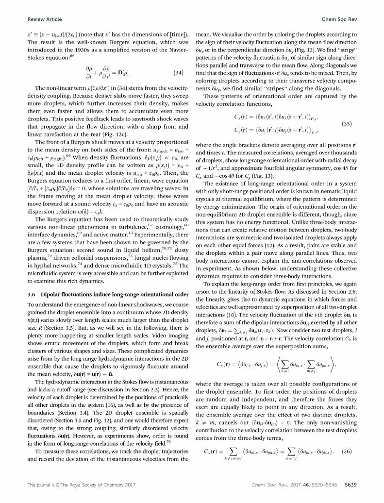
This journal is©The Royal Society of Chemistry 2017 Chem. Soc. Rev., 2017, 46, 5620--5646 | 5639
x0 � (x � uisot)/(2c0) (note that x0 has the dimensions of [time]).The result is the well-known Burgers equation, which wasintroduced in the 1930s as a simplified version of the Navier–Stokes equation:66
@r@tþ r
@r@x0¼ D½r�: (34)
The non-linear term r(qr/qx0) in (34) stems from the velocity-density coupling. Because denser slabs move faster, they sweepmore droplets, which further increases their density, makesthem even faster and allows them to accumulate even moredroplets. This positive feedback leads to sawtooth shock wavesthat propagate in the flow direction, with a sharp front andlinear rarefaction at the rear (Fig. 12c).
The front of a Burgers shock moves at a velocity proportionalto the mean density on both sides of the front: ushock = uiso +c0(rleft + rright).
66 When density fluctuations, dr(x,y) { r0, aresmall, the 1D density profile can be written as r(x,t) = r0 +dr(x,t) and the mean droplet velocity is uiso + c0r0. Then, theBurgers equation reduces to a first-order, linear, wave equation[q/qt + (c0r0)q/qx]dr = 0, whose solutions are traveling waves. Inthe frame moving at the mean droplet velocity, these wavesmove forward at a sound velocity cs = c0r0 and have an acousticdispersion relation o(k) = csk.
The Burgers equation has been used to theoretically studyvarious non-linear phenomena in turbulence,67 cosmology,68
interface dynamics,69 and active matter.13 Experimentally, thereare a few systems that have been shown to be governed by theBurgers equation: second sound in liquid helium,70,71 dustyplasma,72 driven colloidal suspensions,73 fungal nuclei flowingin hyphal networks,74 and dense microfluidic 1D crystals.75 Themicrofluidic system is very accessible and can be further exploitedto examine this rich dynamics.
3.6 Dipolar fluctuations induce long-range orientational order
To understand the emergence of non-linear shockwaves, we coarsegrained the droplet ensemble into a continuum whose 2D densityn(r,t) varies slowly over length scales much larger than the dropletsize R (Section 3.5). But, as we will see in the following, there isplenty more happening at smaller length scales. Video imagingshows erratic movement of the droplets, which form and breakclusters of various shapes and sizes. These complicated dynamicsarise from by the long-range hydrodynamic interactions in the 2Densemble that cause the droplets to vigorously fluctuate aroundthe mean velocity, du(r) = u(r) � %u.
The hydrodynamic interaction in the Stokes flow is instantaneousand lacks a cutoff range (see discussion in Section 2.2). Hence, thevelocity of each droplet is determined by the positions of practicallyall other droplets in the system (16), as well as by the presence ofboundaries (Section 3.4). The 2D droplet ensemble is spatiallydisordered (Section 3.5 and Fig. 12), and one would therefore expectthat, owing to the strong coupling, similarly disordered velocityfluctuations du(r). However, as experiments show, order is foundin the form of long-range correlations of the velocity field.76
To measure these correlations, we track the droplet trajectoriesand record the deviation of the instantaneous velocities from the
mean. We visualize the order by coloring the droplets according tothe sign of their velocity fluctuation along the mean flow directiondux or in the perpendicular direction duy (Fig. 13). We find ‘‘stripy’’patterns of the velocity fluctuation dux of similar sign along direc-tions parallel and transverse to the mean flow. Along diagonals wefind that the sign of fluctuations of dux tends to be mixed. Then, bycoloring droplets according to their transverse velocity compo-nents duy, we find similar ‘‘stripes’’ along the diagonals.
These patterns of orientational order are captured by thevelocity correlation functions,
CxðrÞ ¼ duxðr0; tÞduxðrþ r0; tÞh ir0;t;
CyðrÞ ¼ duyðr0; tÞduyðrþ r0; tÞ�
r0;t;(35)
where the angle brackets denote averaging over all positions r0
and times t. The measured correlations, averaged over thousandsof droplets, show long-range orientational order with radial decayof B1/r2, and approximate fourfold angular symmetry, cos 4y forCx and �cos 4y for Cy (Fig. 13).
The existence of long-range orientational order in a systemwith only short-range positional order is known in nematic liquidcrystals at thermal equilibrium, where the pattern is determinedby energy minimization. The origin of orientational order in thenon-equilibrium 2D droplet ensemble is different, though, sincethis system has no energy functional. Unlike three-body interac-tions that can create relative motion between droplets, two-bodyinteractions are symmetric and two isolated droplets always applyon each other equal forces (12). As a result, pairs are stable andthe droplets within a pair move along parallel lines. Thus, twobody interactions cannot explain the anti-correlations observedin experiment. As shown below, understanding these collectivedynamics requires to consider three-body interactions.
To explain the long-range order from first principles, we againresort to the linearity of Stokes flow. As discussed in Section 2.6,the linearity gives rise to dynamic equations in which forces andvelocities are well-approximated by superposition of all two-dropletinteractions (16). The velocity fluctuation of the i-th droplet dui istherefore a sum of the dipolar interactions duik exerted by all otherdroplets, dui ¼
Pkai duik ri; rkð Þ. Now consider two test droplets, i
and j, positioned at ri and rj = ri + r. The velocity correlation Cx isthe ensemble average over the superposition sums,
CxðrÞ ¼ dui;x � duj;x�
¼Xkai
duik;x �Xmaj
dujm;x
* +;
where the average is taken over all possible configurations ofthe droplet ensemble. To first-order, the positions of dropletsare random and independent, and therefore the forces theyexert are equally likely to point in any direction. As a result,the ensemble average over the effect of two distinct droplets,k a m, cancels out hduik�dujmi = 0. The only non-vanishingcontribution to the velocity correlation between the test dropletscomes from the three-body terms,
CxðrÞ ¼X
kai;maj
duik;x � dujm;x�
¼Xkai; j
duik;x � dujk;x�
: (36)
Review Article Chem Soc Rev
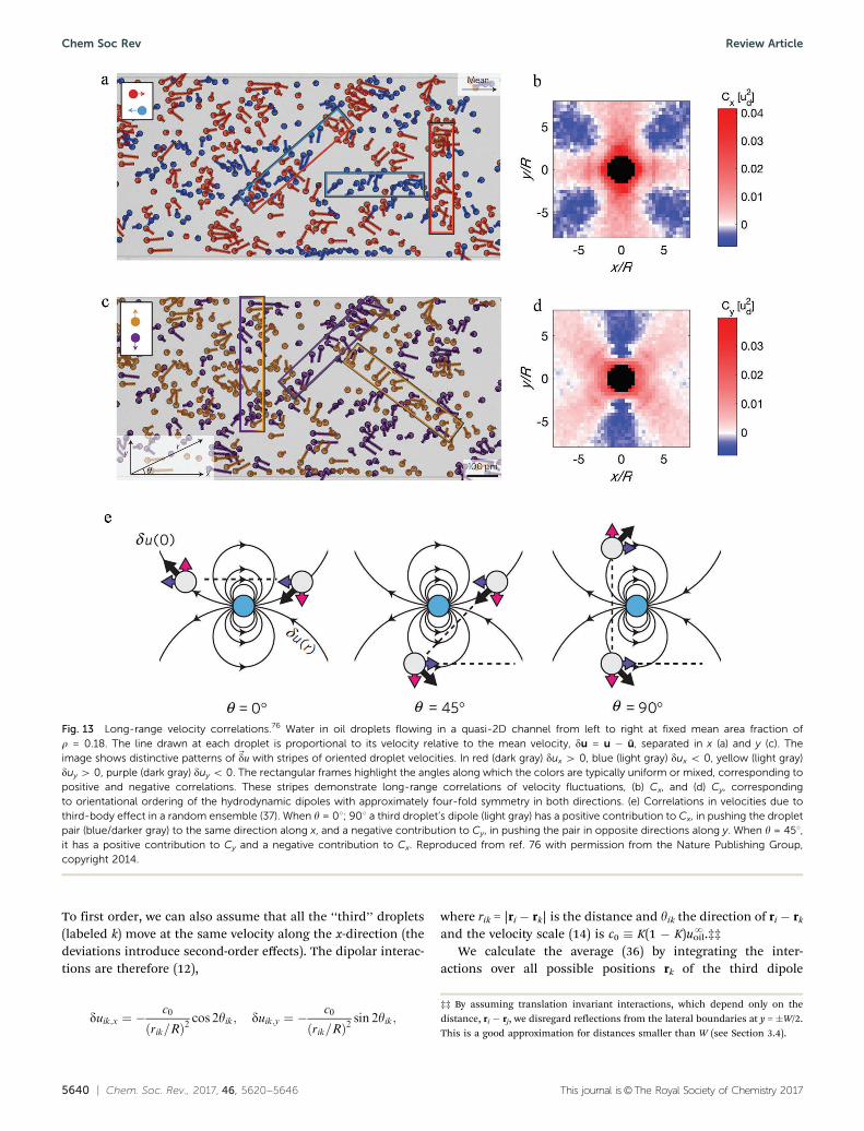
5640 | Chem. Soc. Rev., 2017, 46, 5620--5646 This journal is©The Royal Society of Chemistry 2017
To first order, we can also assume that all the ‘‘third’’ droplets(labeled k) move at the same velocity along the x-direction (thedeviations introduce second-order effects). The dipolar interac-tions are therefore (12),
duik;x ¼ �c0
rik=Rð Þ2cos 2yik; duik;y ¼ �
c0
rik=Rð Þ2sin 2yik;
where rik = |ri � rk| is the distance and yik the direction of ri � rk
and the velocity scale (14) is c0 � K(1 � K)uN
oil.‡‡We calculate the average (36) by integrating the inter-
actions over all possible positions rk of the third dipole
Fig. 13 Long-range velocity correlations.76 Water in oil droplets flowing in a quasi-2D channel from left to right at fixed mean area fraction ofr = 0.18. The line drawn at each droplet is proportional to its velocity relative to the mean velocity, du = u � %u, separated in x (a) and y (c). Theimage shows distinctive patterns of~du with stripes of oriented droplet velocities. In red (dark gray) dux 4 0, blue (light gray) dux o 0, yellow (light gray)duy 4 0, purple (dark gray) duy o 0. The rectangular frames highlight the angles along which the colors are typically uniform or mixed, corresponding topositive and negative correlations. These stripes demonstrate long-range correlations of velocity fluctuations, (b) Cx, and (d) Cy, correspondingto orientational ordering of the hydrodynamic dipoles with approximately four-fold symmetry in both directions. (e) Correlations in velocities due tothird-body effect in a random ensemble (37). When y = 01; 901 a third droplet’s dipole (light gray) has a positive contribution to Cx, in pushing the dropletpair (blue/darker gray) to the same direction along x, and a negative contribution to Cy, in pushing the pair in opposite directions along y. When y = 451,it has a positive contribution to Cy and a negative contribution to Cx. Reproduced from ref. 76 with permission from the Nature Publishing Group,copyright 2014.
‡‡ By assuming translation invariant interactions, which depend only on thedistance, ri � rj, we disregard reflections from the lateral boundaries at y = �W/2.This is a good approximation for distances smaller than W (see Section 3.4).
Chem Soc Rev Review Article
This journal is©The Royal Society of Chemistry 2017 Chem. Soc. Rev., 2017, 46, 5620--5646 | 5641
(using a Fourier transform76), excluding the area where dro-plets cannot overlap,
CxðrÞ ¼ n0
ðduik;x � dujk;xd2rk
¼ n0c02
ðcos 2yikrik=Rð Þ2
� cos 2yjkrjk=R� �2d2rk
¼ r0c02 � cos 4yðr=RÞ2;
(37)
where r0 � pR2n0 is the area density of the droplets. A similarcalculation yields for the y-correlation, Cy(r) = �Cx(r). Theresulting expression (37) recapitulates the salient features ofthe data: long-range orientational order with fourfold symmetry.Intuitively, the positive and negative correlations between twotest droplets are explained by the possible positions of the thirddroplet that represents the ensemble (Fig. 13e). In non-drivensystems, such as thermally fluctuating Brownian particles, thedipole of the third particle is randomly oriented, and the three-body integral (37) vanishes (up to a higher order corrections).37
We see that the significant three-body effect observed in the2D ensemble76 is another manifestation of the symmetrybreaking field.
The origin of the correlations is the interaction of the testdroplets with the surrounding ‘effective medium’. This origin isreflected in (37), which is the spatial autocorrelation of the dipolevelocity field. The correlations scale as Cx(r) = �Cy(r) B r0/r2, likethe dipole field itself. Thus, direct two-body interactions, whichscale as Br0
2/r4, may dominate correlations at short ranges, butbecome negligible as they decay faster than of the effect of themedium at large distances. The significance of the velocityfluctuations is estimated by normalizing the velocity correla-tion with respect to the isolated droplet velocity, which yieldsthe ratio, Cx/uiso
2 B r0K2. In the experiments described inSection 3, K C 0.2, and this ratio is only a few percent. However,experiments with gas bubbles (K = 2) are theoretically expectedto exhibit much stronger effects.
3.7 Periodically driven ensembles in quasi-2D
Experiments on colloidal suspensions under periodic shearflow revealed that when increasing the shear amplitude beyonda critical value, the system undergoes a phase transition from areversible to an irreversible state.92,93 This transition stems froman interplay between reversible hydrodynamic interactions (seeSection 2.2) and irreversible two-body collisions, in which thelatter dominate the dynamics at high shear amplitude. Under-standing the effect of irreversible contact interactions in complexfluids is related to macroscopic rheological phenomena such asshear thinning,94 shear thickening,95 memory96 and dynamicself-assembly.97 The experiments92,93 motivated recent work toinvestigate the response of quasi-2D microfluidic droplets toperiodic, back and forth, driving91,98 (Fig. 14). Interestingly, thereversible to irreversible phase transition is of first-order and isaccompanied by a marked structural change. In shear ampli-tudes smaller than the critical value, the ensemble exhibits long-range structural order corresponding to the coexistence of two
liquid-like phases; in shear amplitudes above the transition thisspatial order is lost.91 Further experimental98 and theoretical99
investigations have shown that the ordered states below thetransition shear amplitude are hyperuniform and that, interest-ingly, their formation does not require the hydrodynamic inter-actions between the droplets.
4 DIY guide to microfluidicexperiments
After exploring the basic physics of microfluidic droplet ensem-ble and the emergent collective modes, we discuss the practicalaspects of how one can build a setup and run experiments toexamine such non-equilibrium phenomena. Our aim is to explainthe essential components and techniques, and the design princi-ples of the setup. The experimental setup for measurements onmicrofluidic droplet ensembles relies on standard techniques:microfluidic device fabrication, matching the driving system andthe fluids, light microscopy, and image analysis.
4.1 The microfluidic device
The device (Fig. 1a) includes an area for droplet formation inwhich oil and water channels meet, in either a T-junction6,26,27
or a flow-focusing geometry.19,77 Downstream the droplet for-mation area, droplets flow into a wider channel where theyform the ensemble. More elaborate droplet generator designsinclude ‘dilution channels’ downstream the droplet formationarea, which add carrier fluid into the main channel to controldroplet density with minimum impact on the droplet formationprocess.78 Design principles for devices based on the T-junctiongeometry are given in ref. 31. The channel layout is designed instandard CAD software and then used to print a mask for photo-lithography. Since the smallest dimension in such devices is10–30 mm, it is enough to use printed transparency masks thatare much cheaper than metal-on-glass mask.
The two methods usually used for fabricating droplet-basedmicrofluidic devices are soft-lithography and silicon patterning.17
Soft lithography is used to make channels made of PDMSelastomer. PDMS channels might be limited in their width-to-height aspect ratio due to the elastomer compliance underpressure. Hence, when a large aspect ratio is required – e.g. toavoid sidewall boundary effects when measuring very largedroplet ensembles – one may fabricate the channels by pattern-ing grooves in hard silicon. In soft-lithography, the mask isused in a standard photolithography process to generate a rigidmold, typically made of an epoxy-based negative photoresist.Photolithography is usually performed in a clean-room facility,although smaller, lab-scale setups may be sufficient. Alterna-tively, the photolithography process can be commercially out-sourced to obtain a mold based on the CAD file. The mold isused for casting PDMS elastomer that, after thermal curing,separating from the mold, and attaching to a flat surface formsthe channels. Hence, a single mold can be used to makemultiple PDMS devices. To obtain stable droplet formationand flow, it is advantageous to fabricate the channels such that
Review Article Chem Soc Rev
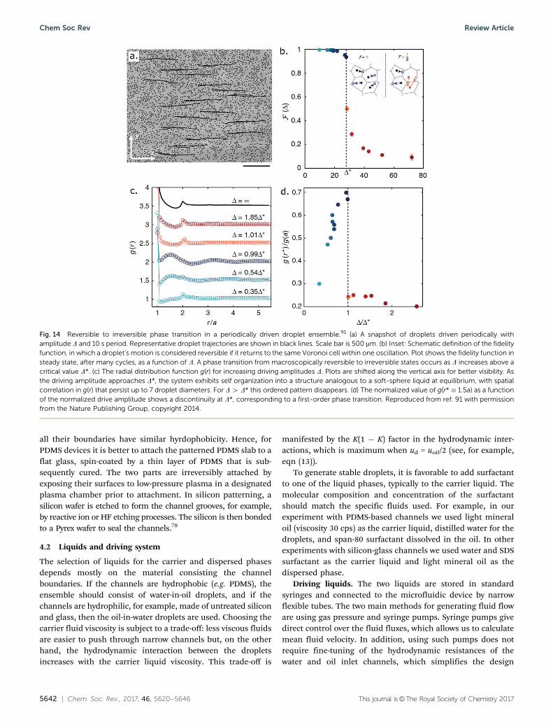
5642 | Chem. Soc. Rev., 2017, 46, 5620--5646 This journal is©The Royal Society of Chemistry 2017
all their boundaries have similar hyrdophobicity. Hence, forPDMS devices it is better to attach the patterned PDMS slab to aflat glass, spin-coated by a thin layer of PDMS that is sub-sequently cured. The two parts are irreversibly attached byexposing their surfaces to low-pressure plasma in a designatedplasma chamber prior to attachment. In silicon patterning, asilicon wafer is etched to form the channel grooves, for example,by reactive ion or HF etching processes. The silicon is then bondedto a Pyrex wafer to seal the channels.78
4.2 Liquids and driving system
The selection of liquids for the carrier and dispersed phasesdepends mostly on the material consisting the channelboundaries. If the channels are hydrophobic (e.g. PDMS), theensemble should consist of water-in-oil droplets, and if thechannels are hydrophilic, for example, made of untreated siliconand glass, then the oil-in-water droplets are used. Choosing thecarrier fluid viscosity is subject to a trade-off: less viscous fluidsare easier to push through narrow channels but, on the otherhand, the hydrodynamic interaction between the dropletsincreases with the carrier liquid viscosity. This trade-off is
manifested by the K(1 � K) factor in the hydrodynamic inter-actions, which is maximum when ud = uoil/2 (see, for example,eqn (13)).
To generate stable droplets, it is favorable to add surfactantto one of the liquid phases, typically to the carrier liquid. Themolecular composition and concentration of the surfactantshould match the specific fluids used. For example, in ourexperiment with PDMS-based channels we used light mineraloil (viscosity 30 cps) as the carrier liquid, distilled water for thedroplets, and span-80 surfactant dissolved in the oil. In otherexperiments with silicon-glass channels we used water and SDSsurfactant as the carrier liquid and light mineral oil as thedispersed phase.
Driving liquids. The two liquids are stored in standardsyringes and connected to the microfluidic device by narrowflexible tubes. The two main methods for generating fluid floware using gas pressure and syringe pumps. Syringe pumps givedirect control over the fluid fluxes, which allows us to calculatemean fluid velocity. In addition, using such pumps does notrequire fine-tuning of the hydrodynamic resistances of thewater and oil inlet channels, which simplifies the design
Fig. 14 Reversible to irreversible phase transition in a periodically driven droplet ensemble.91 (a) A snapshot of droplets driven periodically withamplitude D and 10 s period. Representative droplet trajectories are shown in black lines. Scale bar is 500 mm. (b) Inset: Schematic definition of the fidelityfunction, in which a droplet’s motion is considered reversible if it returns to the same Voronoi cell within one oscillation. Plot shows the fidelity function insteady state, after many cycles, as a function of D. A phase transition from macroscopically reversible to irreversible states occurs as D increases above acritical value D*. (c) The radial distribution function g(r) for increasing driving amplitudes D. Plots are shifted along the vertical axis for better visibility. Asthe driving amplitude approaches D*, the system exhibits self organization into a structure analogous to a soft-sphere liquid at equilibrium, with spatialcorrelation in g(r) that persist up to 7 droplet diameters. For D 4 D* this ordered pattern disappears. (d) The normalized value of g(r* � 1.5a) as a functionof the normalized drive amplitude shows a discontinuity at D*, corresponding to a first-order phase transition. Reproduced from ref. 91 with permissionfrom the Nature Publishing Group, copyright 2014.
Chem Soc Rev Review Article
This journal is©The Royal Society of Chemistry 2017 Chem. Soc. Rev., 2017, 46, 5620--5646 | 5643
process. Using precision pressure regulators to drive the liquidstypically results in smoother flow than a syringe-pump drivenflow, due to fluctuations induced by the pump’s step motor.Also, filling the channel in the beginning of experiment is asimpler process with pressure-driven flow, because the flowrate depends on the hydrodynamic resistance of the filled partof the tubes and channels.
4.3 Imaging and analysis
The microfluidic device is mounted on a standard optical micro-scope, preferably with a motorized translation stage to allowimaging the droplets while moving in their frame of reference.Droplets are filmed by a camera mounted on the microscope. Thetypical frequency scales like Cs/r E 1–10 Hz. For this reason, andsince the fluctuations in droplet velocity with respect to theirmean velocity are typically tens of mm, the camera frame rate canbe relatively low, about tens of frames-per-second. The requiredfield of view is mostly determined by the typical droplet diameter.For example, for measuring the phonon spectra of a 1D crystalrequires tracking at least a few tens of droplets for at least 20 s.For droplets with a typical 20–30 mm diameter and a similarcrystal spacing, the length of the field of view is 1000–3000 mm,which implies a small magnification of �5 or �10 and a field ofview of 1–2 mm.
Image analysis is performed by software that tracks the center ofeach droplet and identifies droplet trajectories. Because the dropletsare round discs of uniform size, such image analysis task is notcomplicated. One method for identifying a droplet center relieson the fact that the droplets appear as round dark rings, oftenwith a brighter interior than the channel (the latter depends onthe position of the droplet with respect to the focal plane). Thecharacteristic ring shape can be fitted to a pre-determined profilewith its x and y positions being free parameters (a method knownas the ‘Moses-Abadi’ algorithm). The imaged droplet size in pixelsshould be large enough to allow accurate tracking of their centers,which is important, for example, for measuring clean phononspectra.
5 Conclusions, overview andperspective5.1 Dimension, divergence and scale invariance
The microfluidic droplet ensemble proved to be a convenientmodel to examine collective motion in a far-from-equilibrium,dissipative system governed by long-range interactions. Withinthis wide class of systems, the microfluidic ensemble mostresembles the sedimentation of non-Brownian particles in a 3Dfluid under gravity.43,48,49 Theoretically, the complex collectivedynamics in sedimentation46,47,79–81 remains obscure due to thesumming of the 1/r inter-particle forces in 3D, which divergeswith the system size.45
In contrast, the 1/r2 forces in the quasi-2D droplet ensembleare a borderline case between additive and non-additive systems,since their exponent of decay is the same as the ensembledimension. This marginal non-additivity and scale invariance
cure the system from the power-law divergence seen in 3D andrenders it theoretically tractable (Section 2.8). In addition, pro-pagating modes in a highly dissipative system, which are a prioriover-damped, can be sustained by a symmetry-breaking drivingfield (Section 3.1).
In this mini-review, we showed from first principles how thelong-range dipolar interactions between the droplets lead tocollective modes such as phonons, shockwaves, and velocitycorrelations. The quasi-2D droplet ensemble is, therefore, a con-venient model system for studying non-equilibrium physics.6,7
Indeed, similar long-range hydrodynamics have been shown togovern the collective dynamics of other quasi-2D systems, withvarious types of particles and geometries:� 1D structures. The collective modes of the 1D droplet
crystal were further investigated to elucidate the dynamics underpositional perturbations, showing how density shock wavespropagate along the crystal82 and how distinct phonon modescan be excited and analyzed (Fig. 8b).55 In addition, the instabi-lity of the microfluidic crystal has been numerically analyzed,showing nonlinear mode coupling that promotes the instability.83
Numerical methods have also been used to calculate the phononspectra in a crystal of spheres in quasi-2D flow, which are verysimilar to the spectra of the microfluidic ‘pancake’ crystal54
(Fig. 8a).Similar phonons were observed also in a different geometry of
a 1D ring of colloidal micro-particles driven in an optical trap10
(Fig. 1d and 8c). The spectra of these phonons conserve theoverall sine-like shape of their microfluidics counterparts,although the hydrodynamic interaction between the particles isdominated by the 1/r momentum monopole. Interestingly, thecurvature of the optical trap induces pairwise attraction betweenparticles,84 in contrast to an isolated pair of microfluidic droplets,which do not attract not repel each other (Fig. 3). The ‘peloton’effect of the microfluidics crystal has been shown to be applicablein the collective motion of red blood cells flowing in narrowcapillaries12 (Fig. 1f).� 2D ensembles. Collective modes in ordered 2D ensembles
have been numerically analyzed in a cubic crystal of spheres inquasi-2D,54 and the phonon spectra in the five 2D Bravaislattices have been analytically calculated.85 Works on disordered2D ensembles have elucidated the full 2D spectrum of densitywaves,78 and reported Burgers shockwave dynamics in droplet’traffic jams’,82 colloids in AC field,73 and even in fungal nucleiflowing in hyphal networks.74
� Clusters of droplets or particles. Hydrodynamic interac-tions in quasi-2D have been shown to govern processes ofclustering and self-assembly of droplets or micro-particles inmicrofluidic channels. The motion of small droplet clustershave been measured35 and simulated numerically,86 and thehydrodynamic interactions between droplets have been usedto form and polymerize small clusters of specific shapes.11
Further, non-spherical particles, such as dumbbells, have beenfabricated within a microfluidic channel and their trajectorieshave been measured and analyzed based on the dipolar theory.Similar framework has been used to numerically analyze thedynamics of ensembles of such particles.
Review Article Chem Soc Rev
5644 | Chem. Soc. Rev., 2017, 46, 5620--5646 This journal is©The Royal Society of Chemistry 2017
� Active particles. Ensembles of active particles moving inquasi-2D or near a boundary of a 3D fluid have the propensityfor exhibiting even richer phenomena that passive particles,such as droplets dragged by an imposed flow. The main reasonis that the flow field of each active particle can have arbitrarydirection, whereas the dipoles of passive droplet are all parallelto the imposed flow (up to negligible transverse velocity). Activeparticles belong to the wider classes of active matter and micro-swimmers.87 For example, hydrodynamic interactions in quasi-2Densembles also affect the collective dynamics of active particles,85
self-propelled droplets,88 and micro-swimmers89 that have beenshown to exhibit Burgers shockwaves dynamics.13,90 Recent workshowed that hydrodynamic interactions promote the emergenceof collective motion in populations of motile colloids and micro-rollers near a surface.14,15
5.2 Perspective
The microfluidic droplet ensemble is a convenient experimentaland theoretical platform to study various non-equilibrium pheno-mena. Here, we reviewed works which demonstrated the use ofmicrofluidic ensemble to observe and explain the emergence ofcollective modes in dissipative far-from-equilibrium systems.However, these are only the first steps and are still many openquestions and directions.
Several immediate open questions are the following: first, theinstability modes of the 1D microfluidic crystal are unexplained. Inparticular, the nonlinear mechanisms that drives this instabilityand the coupled wavelengths involved are unknown. In addition,it may be interesting to excite particular phonons and map theirnonlinear coupling to other modes. Second, the 2D disorderedensemble exhibits complex clustering dynamics, in whichclusters of droplets continuously form and break. Clusteringdynamics is most pronounced when the depletion forcessticking droplets together are of the same order of magnitudeas the hydrodynamic interactions. This rich dynamical processmay lead to new insights in non-equilibrium statistical mechanics.Interestingly, clustering processes are governed by the near-fieldhydrodynamic interactions, where the dipolar approximation isless accurate.
Given the phenomena demonstrated so far, we believe thatdriven microfluidic ensembles can be a convenient tool toaddress longstanding problems in non-equilibrium science: the2D ensemble may offer an opportunity to understand the role ofmoving boundaries in the time-irreversibility of fluid system, inparticular in the low-Re regime, where the Stokes equation istime-reversible. Moreover, observation the multi-scale many-bodydynamics of a large ensembles, it is possible to track howthe emergence of irreversibility is related to the transfer ofmomentum and energy between different spatial and temporalscales. For example, we hypothesize that studying the relationbetween reversible Stokes hydrodynamics and irreversible contactinteractions under constant, rather than periodic, drive, may revealnew mechanisms of pattern formation. These directions arealso related to questions concerning the emergence of dynamicmemory, the effect of external feedback and many-body informationengines. Microfluidics may be also useful to study topological
phenomena in non-equilibrium many-body systems, such as thedynamical phase transitions.100 Finally, microfluidic ensemblescould be used to probe the existence of extremum principles innon-equilibrium systems.101 We propose that monitoring thedissipation rate in a quasi-2D ensemble that is perturbed fromits steady-state motion, may provide insight on the existence ofa minimization principle underlying the collective dynamics.
Conflicts of interest
There are no conflicts of interest to declare.
Acknowledgements
T. B. was supported by the Faculty Fellowship of the AzrieliFellows Program. T. T. was supported by the Institute for BasicScience IBS-R020.
References
1 D. Ruelle, J. Stat. Phys., 1999, 95, 393–468.2 G. Gallavotti and E. G. Cohen, J. Stat. Phys., 1995, 80,
931–970.3 C. Jarzynski, Phys. Rev. Lett., 1997, 78, 2690.4 A. Campa, T. Dauxois and S. Ruffo, Phys. Rep., 2009, 480,
57–159.5 M. C. Cross and P. C. Hohenberg, Rev. Mod. Phys., 1993, 65,
851–1112.6 T. Beatus, T. Tlusty and R. Bar-Ziv, Nat. Phys., 2006, 2, 743.7 P. Garstecki and R. Hołyst, Nat. Phys., 2015, 11, 305–306.8 T. Beatus, T. Tlusty and R. Bar-Ziv, Phys. Rev. Lett., 2009,
103, 114502.9 W. E. Uspal, H. B. Eral and P. S. Doyle, Nat. Commun., 2013,
4, 2666.10 H. Nagar and Y. Roichman, Phys. Rev. E: Stat., Nonlinear,
Soft Matter Phys., 2014, 90, 042302.11 B. Shen, J. Ricouvier, F. Malloggi and P. Tabeling, Adv. Sci.,
2016, 3, 1600012.12 J. L. McWhirter, H. Noguchi and G. Gompper, Proc. Natl.
Acad. Sci. U. S. A., 2009, 106, 6039–6043.13 A. C. H. Tsang and E. Kanso, Phys. Rev. Lett., 2016,
116, 048101.14 A. Bricard, J.-B. Caussin, N. Desreumaux, O. Dauchot and
D. Bartolo, Nature, 2013, 503, 95–98.15 M. Driscoll, B. Delmotte, M. Youssef, S. Sacanna, A. Donev
and P. Chaikin, Nat. Phys., 2016, 375–379.16 H. A. Stone, A. D. Stroock and A. Ajdari, Annu. Rev. Fluid
Mech., 2004, 36, 381–411.17 T. M. Squires and S. R. Quake, Rev. Mod. Phys., 2005, 77,
977–1026.18 A. Gonther and K. Jensen, Lab Chip, 2006, 6, 1487–1503.19 G. F. Christopher and S. L. Anna, J. Phys. D: Appl. Phys.,
2007, 40, 319–336.20 L. Shui, J. Eijkel and A. van den Berg, Adv. Colloid Interface
Sci., 2007, 133, 35–49.
Chem Soc Rev Review Article
This journal is©The Royal Society of Chemistry 2017 Chem. Soc. Rev., 2017, 46, 5620--5646 | 5645
21 S. Teh, R. Lin, L. Hung and A. Lee, Lab Chip, 2008, 8,198–220.
22 P. Tabeling, Lab Chip, 2009, 9, 2428–2436.23 C. Baroud, F. Gallaire and R. Dangla, Lab Chip, 2010, 10,
2032–2045.24 R. Pompano, W. Liu, W. Du and R. Ismagilov, Annu. Rev.
Anal. Chem., 2011, 4, 59–81.25 R. Seemann, M. Brinkmann, T. Pfohl and S. Herminghaus,
Rep. Prog. Phys., 2012, 75, 16601.26 T. Thorsen, R. W. Roberts, F. H. Arnold and S. R. Quake,
Phys. Rev. Lett., 2001, 86, 4163–4166.27 P. Garstecki, M. Fuerstman, H. Stone and G. Whitesides,
Lab Chip, 2006, 6, 437–446.28 E. M. Purcell, Am. J. Phys., 1977, 45, 3–11.29 E. Guyon, J. P. Hulin, L. Petit and C. D. Mitescu, Physical
hydrodynamics, Oxford University Press, Oxford, 2nd edn,2015, p. xvii.
30 L. D. Landau and E. Lifshitz, Fluid mechanics, Oxford,Pergamon, 1987.
31 T. Beatus, R. H. Bar-Ziv and T. Tlusty, Phys. Rep., 2012, 516,103–145.
32 B. Cui, H. Diamant, B. Lin and S. A. Rice, Phys. Rev. Lett.,2004, 92, 258301.
33 G. Taylor and P. Saffman, Q. J. Mech. Appl. Math., 1959, 12,265–279.
34 R. Dangla, S. Lee and C. Baroud, Phys. Rev. Lett., 2011,107, 124501.
35 B. Shen, M. Leman, M. Reyssat and P. Tabeling, Exp.Fluids, 2014, 55, 1728.
36 V. Y. Mazur, Izv. Akad. Nauk SSSR, Mekh. Zhidk. Gaza, 1970,6, 80–84.
37 H. Diamant, B. Cui, B. Lin and S. Rice, J. Phys.: Condens.Matter, 2005, 17, S2787.
38 H. Diamant, J. Phys. Soc. Jpn., 2009, 78, 041002.39 G. G. Stokes, Trans. Cambridge Philos. Soc., 1851, 9, 8.40 J. Happel and H. Brenner, Low Reynolds Number Hydro-
dynamics, Kluwer, Boston, 1965.41 L. Onsager, Nuovo Cimento, 1949, 6, 279–287.42 L. M. Pismen, Vortices in nonlinear fields: From liquid
crystals to superfluids, from non-equilibrium patterns tocosmic strings, Oxford University Press, 1999, vol. 100.
43 S. Ramaswamy, Adv. Phys., 2001, 50, 297–341.44 R. E. Caflisch and J. H. C. Luke, Phys. Fluids, 1985, 28,
759–760.45 G. K. Batchelor, J. Fluid Mech., 1972, 52, 245–268.46 P. N. Segre, E. Herbolzheimer and P. M. Chaikin, Phys. Rev.
Lett., 1997, 79, 2574–2577.47 M. P. Brenner, Phys. Fluids, 1999, 11, 754–772.48 E. Guazzelli and J. Hinch, Annu. Rev. Fluid Mech., 2011, 43,
97–116.49 E. Guazzelli, C. R. Mec., 2006, 334, 539–544.50 L. D. Landau and E. M. Lifshitz, Electrodynamics of
Continuous Media, Pergamon Press, 1960.51 M. Polin, D. G. Grier and S. R. Quake, Phys. Rev. Lett., 2006,
96, 088101.52 J. M. Crowley, J. Fluid Mech., 1971, 45, 151–159.
53 R. A. Simha and S. Ramaswamy, Phys. Rev. Lett., 1999,83, 3285.
54 M. Baron, J. Bławzdziewicz and E. Wajnryb, Phys. Rev. Lett.,2008, 100, 174502.
55 U. D. Schiller, J.-B. Fleury, R. Seemann and G. Gompper,Soft Matter, 2015, 11, 5850–5861.
56 S. Novikov, S. A. Rice, B. Cui, H. Diamant and B. Lin, Phys.Rev. E: Stat., Nonlinear, Soft Matter Phys., 2010, 82, 031403.
57 G. R. Kirchhoff, Poggend. Annal., 1845, 64, 487–514.58 X. Xu, S. A. Rice, B. Lin and H. Diamant, Phys. Rev. Lett.,
2005, 95, 158301.59 T. Beatus, R. Bar-Ziv and T. Tlusty, Phys. Rev. Lett., 2007,
99, 124502.60 R. P. Feynman, R. Leighton and M. Sands, The Feynman
lectures on physics, Reading, MA, Addison-Wesley, 1963,vol. 2, pp. 7–5.
61 B. Cui, H. Diamant and B. Lin, Phys. Rev. Lett., 2002,89, 188302.
62 D. Frydel and H. Diamant, Phys. Rev. Lett., 2010, 104, 248302.63 E. Kosheleva, B. Leahy, H. Diamant, B. Lin and S. A. Rice,
Phys. Rev. E: Stat., Nonlinear, Soft Matter Phys., 2012, 86,041402.
64 B. Lin, B. Cui, X. Xu, R. Zangi, H. Diamant and S. A. Rice, Phys.Rev. E: Stat., Nonlinear, Soft Matter Phys., 2014, 89, 022303.
65 T. Tlusty, Macromolecules, 2006, 39, 3927–3930.66 J. M. Burgers, The nonlinear diffusion equation. Asymptotic
solutions and statistical problems, D. Reidel PublishingCompany, Dordrecht, Boston, 1974.
67 J. Bec and K. Khanin, Phys. Rep., 2007, 447, 1–66.68 Y. B. Zel’Dovich, Astron. Astrophys., 1970, 5, 84–89.69 M. Kardar, G. Parisi and Y. C. Zhang, Phys. Rev. Lett., 1986,
56, 889–892.70 L. S. Goldner, N. Mulders and G. Ahlers, J. Low Temp. Phys.,
1993, 93, 131–182.71 S. Kitabatake and Y. Sawada, J. Phys. Soc. Jpn., 1978, 45, 345.72 S. Ghosh, S. Sarkar, M. Khan, K. Avinash and M. R. Gupta,
Phys. Plasmas, 2003, 10, 977–983.73 C. L. Perez and J. D. Posner, Langmuir, 2010, 26,
9261–9268.74 P. C. Hickey, H. Dou, S. Foshe and M. Roper, arXiv, 2016,
1601.06097.75 N. Champagne, E. Lauga and D. Bartolo, Soft Matter, 2011,
7, 11082–11085.76 I. Shani, T. Beatus, R. H. Bar-Ziv and T. Tlusty, Nat. Phys.,
2014, 10, 140–144.77 S. L. Anna, N. Bontoux and H. A. Stone, Appl. Phys. Lett.,
2003, 82, 364–366.78 N. Desreumaux, J.-B. Caussin, R. Jeanneret, E. Lauga and
D. Bartolo, Phys. Rev. Lett., 2013, 111, 118301.79 G. J. Kynch, Trans. Faraday Soc., 1952, 48, 166–176.80 P. N. Segre, F. Liu, P. Umbanhowar and D. A. Weitz, Nature,
2001, 409, 594–597.81 S. Tee, P. Mucha, L. Cipelletti, S. Manley, M. Brenner,
P. Segre and D. Weitz, Phys. Rev. Lett., 2002, 89, 54501.82 N. Champagne, R. Vasseur, A. Montourcy and D. Bartolo,
Phys. Rev. Lett., 2010, 105, 044502.
Review Article Chem Soc Rev
5646 | Chem. Soc. Rev., 2017, 46, 5620--5646 This journal is©The Royal Society of Chemistry 2017
83 B. Liu, J. Goree and Y. Feng, Phys. Rev. E: Stat., Nonlinear,Soft Matter Phys., 2012, 86, 046309.
84 Y. Sokolov, D. Frydel, D. G. Grier, H. Diamant andY. Roichman, Phys. Rev. Lett., 2011, 107, 158302.
85 N. Desreumaux, N. Florent, E. Lauga and D. Bartolo, Eur.Phys. J. E: Soft Matter Biol. Phys., 2012, 35, 1–11.
86 W. E. Uspal and P. S. Doyle, Soft Matter, 2012, 8, 10676–10686.87 J. Elgeti, R. G. Winkler and G. Gompper, Rep. Prog. Phys.,
2015, 78, 056601.88 R. Seemann, J.-B. Fleury and C. C. Maass, Eur. Phys. J.: Spec.
Top., 2016, 225, 2227–2240.89 T. Brotto, J.-B. Caussin, E. Lauga and D. Bartolo, Phys. Rev.
Lett., 2013, 110, 038101.90 A. Lefauve and D. Saintillan, Phys. Rev. E: Stat., Nonlinear,
Soft Matter Phys., 2014, 89, 021002.91 R. Jeanneret and D. Bartolo, Nat. Commun., 2014, 5, 3474.92 D. Pine, J. P. Gollub, J. Brady and A. Leshansky, Nature,
2005, 438, 997.
93 L. Corte, P. Chaikin, J. P. Gollub and D. Pine, Nat. Phys.,2008, 4, 420.
94 N. Y. Lin, B. M. Guy, M. Hermes, C. Ness, J. Sun, W. C.Poon and I. Cohen, Phys. Rev. Lett., 2015, 115, 228304.
95 J. F. Brady and J. F. Morris, J. Fluid Mech., 1997, 348,103–139.
96 J. D. Paulsen, N. C. Keim and S. R. Nagel, Phys. Rev. Lett.,2014, 113, 068301.
97 W. Lee, H. Amini, H. A. Stone and D. Di Carlo, Proc. Natl.Acad. Sci. U. S. A., 2010, 107, 22413–22418.
98 J. H. Weijs, R. Jeanneret, R. Dreyfus and D. Bartolo, Phys.Rev. Lett., 2015, 115, 108301.
99 E. Tjhung and L. Berthier, Phys. Rev. Lett., 2015, 114,148301.
100 Y. M. Bunkov and H. Godfrin, Topological defects and thenon-equilibrium dynamics of symmetry breaking phase transi-tions, Springer Science & Business Media, 2012, vol. 549.
101 L. Martyushev and V. Seleznev, Phys. Rep., 2006, 426, 1–45.
Chem Soc Rev Review Article